Introduction to SQL

SQL is a standard language for accessing and manipulating databases.

What is SQL?

SQL stands for Structured Query Language

SQL lets you access and manipulate databases

SQL is an ANSI (American National Standards Institute) standard

What Can SQL do?

SQL can execute queries against a database

SQL can retrieve data from a database

SQL can insert records in a database

SQL can update records in a database

SQL can delete records from a database

SQL can create new databases

SQL can create new tables in a database

SQL can create stored procedures in a database

SQL can create views in a database

SQL can set permissions on tables, procedures, and views

SQL is a Standard - BUT....

Although SQL is an ANSI (American National Standards Institute) standard, there are different

versions of the SQL language.

However, to be compliant with the ANSI standard, they all support at least the major commands

(such as SELECT, UPDATE, DELETE, INSERT, WHERE) in a similar manner.

Note: Most of the SQL database programs also have their own proprietary extensions in addition to the SQL standard!

Introduction to SQL

Structure Query Language(SQL) is a programming language used for storing and managing data

in RDBMS. SQL was the first commercial language introduced for E.F

Codd's Relational model. Today almost all RDBMS(MySql, Oracle, Infomix, Sybase, MS

Access) uses SQL as the standard database language. SQL is used to perform all type of data

operations in RDBMS.

SQL Command

SQL defines following data languages to manipulate data of RDBMS.

DDL : Data Definition Language

All DDL commands are auto-committed. That means it saves all the changes permanently in the

database.

Command Description

create to create new table or database

alter for alteration

truncate delete data from table

drop to drop a table

rename to rename a table

DML : Data Manipulation Language

DML commands are not auto-committed. It means changes are not permanent to database, they

can be rolled back.

Command Description

insert to insert a new row

update to update existing row

delete to delete a row

merge merging two rows or two tables

TCL : Transaction Control Language

These commands are to keep a check on other commands and their affect on the database. These

commands can annul changes made by other commands by rolling back to original state. It can

also make changes permanent.

Command Description

commit to permanently save

rollback to undo change

savepoint to save temporarily

DCL : Data Control Language

Data control language provides command to grant and take back authority.

Command Description

grant grant permission of right

revoke take back permission.

DQL : Data Query Language

Command Description

select retrieve records from one or more table

SQL SELECT Statement:

SELECT column1, column2....columnN

FROM table_name;

SQL DISTINCT Clause:

SELECT DISTINCT column1, column2....columnN

FROM table_name;

SQL WHERE Clause:

SELECT column1, column2....columnN

FROM table_name

WHERE CONDITION;

SQL AND/OR Clause:

SELECT column1, column2....columnN

FROM table_name

WHERE CONDITION-1 {AND|OR} CONDITION-2;

SQL IN Clause:

SELECT column1, column2....columnN

FROM table_name

WHERE column_name IN (val-1, val-2,...val-N);

SQL BETWEEN Clause:

SELECT column1, column2....columnN

FROM table_name

WHERE column_name BETWEEN val-1 AND val-2;

SQL LIKE Clause:

SELECT column1, column2....columnN

FROM table_name

WHERE column_name LIKE { PATTERN };

SQL ORDER BY Clause:

SELECT column1, column2....columnN

FROM table_name

WHERE CONDITION

ORDER BY column_name {ASC|DESC};

SQL GROUP BY Clause:

SELECT SUM(column_name)

FROM table_name

WHERE CONDITION

GROUP BY column_name;

SQL COUNT Clause:

SELECT COUNT(column_name)

FROM table_name

WHERE CONDITION;

SQL HAVING Clause:

SELECT SUM(column_name)

FROM table_name

WHERE CONDITION

GROUP BY column_name

HAVING (arithematic function condition);

SQL General Data Types

Each column in a database table is required to have a name and a data type.

SQL developers have to decide what types of data will be stored inside each and every table

column when creating a SQL table. The data type is a label and a guideline for SQL to

understand what type of data is expected inside of each column, and it also identifies how SQL

will interact with the stored data.

The following table lists the general data types in SQL:

Data type Description

CHARACTER(n) Character string. Fixed-length n

VARCHAR(n) or

CHARACTER VARYING(n)

Character string. Variable length. Maximum length n

BINARY(n) Binary string. Fixed-length n

BOOLEAN Stores TRUE or FALSE values

VARBINARY(n) or

BINARY VARYING(n)

Binary string. Variable length. Maximum length n

INTEGER(p) Integer numerical (no decimal). Precision p

SMALLINT Integer numerical (no decimal). Precision 5

INTEGER Integer numerical (no decimal). Precision 10

BIGINT Integer numerical (no decimal). Precision 19

DECIMAL(p,s) Exact numerical, precision p, scale s. Example: decimal(5,2) is a

number that has 3 digits before the decimal and 2 digits after the

decimal

NUMERIC(p,s) Exact numerical, precision p, scale s. (Same as DECIMAL)

FLOAT(p) Approximate numerical, mantissa precision p. A floating number in

base 10 exponential notation. The size argument for this type

consists of a single number specifying the minimum precision

REAL Approximate numerical, mantissa precision 7

FLOAT Approximate numerical, mantissa precision 16

DOUBLE PRECISION Approximate numerical, mantissa precision 16

DATE Stores year, month, and day values

TIME Stores hour, minute, and second values

TIMESTAMP Stores year, month, day, hour, minute, and second values

INTERVAL Composed of a number of integer fields, representing a period of

time, depending on the type of interval

ARRAY A set-length and ordered collection of elements

MULTISET A variable-length and unordered collection of elements

XML Stores XML data

SQL Data Type Quick Reference

However, different databases offer different choices for the data type definition.

The following table shows some of the common names of data types between the various

database platforms:

Data type Access SQLServer Oracle MySQL PostgreSQL

boolean Yes/No Bit Byte N/A Boolean

integer Number

(integer)

Int Number Int

Integer

Int

Integer

float Number

(single)

Float

Real

Number Float Numeric

currency Currency Money N/A N/A Money

string (fixed) N/A Char Char Char Char

string

(variable)

Text

(<256)

Memo

(65k+)

Varchar Varchar

Varchar2

Varchar Varchar

binary object OLE

Object

Memo

Binary

(fixed up to

8K)

Varbinary

(<8K)

Image

(<2GB)

Long

Raw

Blob

Text

Binary

Varbinary

DDL Commands

create command

create is a DDL command used to create a table or a database.

Creating a Database

To create a database in RDBMS, create command is uses. Following is the Syntax,

create database database-name;

Example for Creating Database

create database Test;

The above command will create a database named Test.

Creating a Table

create command is also used to create a table. We can specify names and datatypes of various

columns along.Following is the Syntax,

create table table-name

{

column-name1 datatype1,

column-name2 datatype2,

column-name3 datatype3,

column-name4 datatype4

};

create table command will tell the database system to create a new table with given table name

and column information.

Example for creating Table

create table Student(id int, name varchar, age int);

The above command will create a new table Student in database system with 3 columns, namely

id, name and age.

alter command

alter command is used for alteration of table structures. There are various uses

of alter command, such as,

to add a column to existing table

to rename any existing column

to change datatype of any column or to modify its size.

alter is also used to drop a column.

To Add Column to existing Table

Using alter command we can add a column to an existing table. Following is the Syntax,

alter table table-name add(column-name datatype);

Here is an Example for this,

alter table Student add(address char);

The above command will add a new column address to the Student table

To Add Multiple Column to existing Table

Using alter command we can even add multiple columns to an existing table. Following is the

Syntax,

alter table table-name add(column-name1 datatype1, column-name2 datatype2, column-name

3 datatype3);

Here is an Example for this,

alter table Student add(father-name varchar(60), mother-name varchar(60), dob date);

The above command will add three new columns to the Student table

To Add column with Default Value

alter command can add a new column to an existing table with default values. Following is the

Syntax,

alter table table-name add(column-name1 datatype1 default data);

Here is an Example for this,

alter table Student add(dob date default '1-Jan-99');

The above command will add a new column with default value to the Student table

To Modify an existing Column

alter command is used to modify data type of an existing column . Following is the Syntax,

alter table table-name modify(column-name datatype);

Here is an Example for this,

alter table Student modify(address varchar(30));

The above command will modify address column of the Student table

To Rename a column

Using alter command you can rename an existing column. Following is the Syntax,

alter table table-name rename old-column-name to column-name;

Here is an Example for this,

alter table Student rename address to Location;

The above command will rename address column to Location.

To Drop a Column

alter command is also used to drop columns also. Following is the Syntax,

alter table table-name drop(column-name);

Here is an Example for this,

alter table Student drop(address);

The above command will drop address column from the Student table

SQL queries to Truncate, Drop or Rename a Table

truncate command

truncate command removes all records from a table. But this command will not destroy the

table's structure. When we apply truncate command on a table its Primary key is initialized.

Following is its Syntax,

truncate table table-name

Here is an Example explaining it.

truncate table Student;

The above query will delete all the records of Student table.

truncate command is different from delete command. delete command will delete all the rows

from a table whereas truncate command re-initializes a table(like a newly created table).

For eg. If you have a table with 10 rows and an auto_increment primary key, if you

use delete command to delete all the rows, it will delete all the rows, but will not initialize the

primary key, hence if you will insert any row after using delete command, the auto_increment

primary key will start from 11. But in case of truncatecommand, primary key is re-initialized.

drop command

drop query completely removes a table from database. This command will also destroy the table

structure. Following is its Syntax,

drop table table-name

Here is an Example explaining it.

drop table Student;

The above query will delete the Student table completely. It can also be used on Databases. For

Example, to drop a database,

drop database Test;

The above query will drop a database named Test from the system.

rename query

rename command is used to rename a table. Following is its Syntax,

rename table old-table-name to new-table-name

Here is an Example explaining it.

rename table Student to Student-record;

The above query will rename Student table to Student-record.

DML command

Data Manipulation Language (DML) statements are used for managing data in database. DML

commands are not auto-committed. It means changes made by DML command are not

permanent to database, it can be rolled back.

1) INSERT command

Insert command is used to insert data into a table. Following is its general syntax,

INSERT into table-name values(data1,data2,..)

Lets see an example,

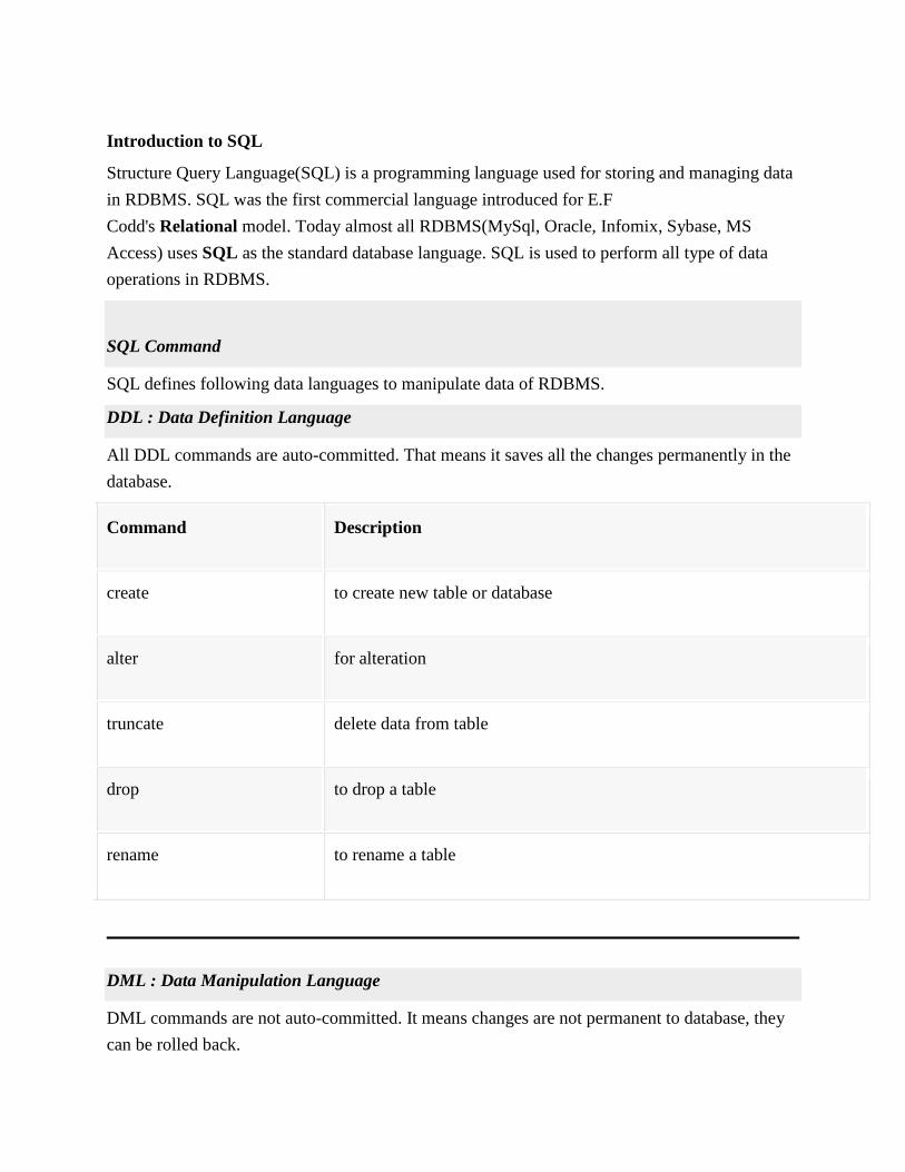
Consider a table Student with following fields.

S_id S_Name age

INSERT into Student values(101,'Adam',15);

The above command will insert a record into Student table.

S_id S_Name age

101 Adam 15

Example to Insert NULL value to a column

Both the statements below will insert NULL value into age column of the Student table.

INSERT into Student(id,name) values(102,'Alex');

Or,

INSERT into Student values(102,'Alex',null);

The above command will insert only two column value other column is set to null.

S_id S_Name age

101 Adam 15

102 Alex

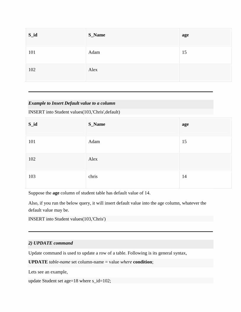
Example to Insert Default value to a column

INSERT into Student values(103,'Chris',default)

S_id S_Name age

101 Adam 15

102 Alex

103 chris 14

Suppose the age column of student table has default value of 14.

Also, if you run the below query, it will insert default value into the age column, whatever the

default value may be.

INSERT into Student values(103,'Chris')

2) UPDATE command

Update command is used to update a row of a table. Following is its general syntax,

UPDATE table-name set column-name = value where condition;

Lets see an example,

update Student set age=18 where s_id=102;

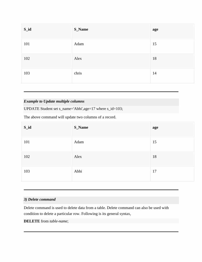
S_id S_Name age

101 Adam 15

102 Alex 18

103 chris 14

Example to Update multiple columns

UPDATE Student set s_name='Abhi',age=17 where s_id=103;

The above command will update two columns of a record.

S_id S_Name age

101 Adam 15

102 Alex 18

103 Abhi 17

3) Delete command

Delete command is used to delete data from a table. Delete command can also be used with

condition to delete a particular row. Following is its general syntax,

DELETE from table-name;

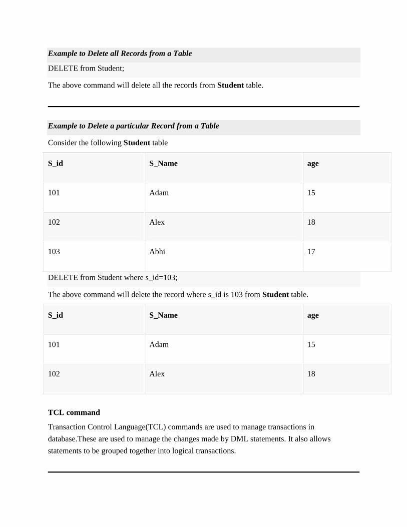
Example to Delete all Records from a Table

DELETE from Student;

The above command will delete all the records from Student table.

Example to Delete a particular Record from a Table

Consider the following Student table

S_id S_Name age

101 Adam 15

102 Alex 18

103 Abhi 17

DELETE from Student where s_id=103;

The above command will delete the record where s_id is 103 from Student table.

S_id S_Name age

101 Adam 15

102 Alex 18

TCL command

Transaction Control Language(TCL) commands are used to manage transactions in

database.These are used to manage the changes made by DML statements. It also allows

statements to be grouped together into logical transactions.

Commit command

Commit command is used to permanently save any transaaction into database.

Following is Commit command's syntax,

commit;

Rollback command

This command restores the database to last commited state. It is also use with savepoint

command to jump to a savepoint in a transaction.

Following is Rollback command's syntax,

rollback to savepoint-name;

Savepoint command

savepoint command is used to temporarily save a transaction so that you can rollback to that

point whenever necessary.

Following is savepoint command's syntax,

savepoint savepoint-name;

Example of Savepoint and Rollback

Following is the class table,

ID NAME

1 abhi

2 adam

4 alex

Lets use some SQL queries on the above table and see the results.

INSERT into class values(5,'Rahul');

commit;

UPDATE class set name='abhijit' where id='5';

savepoint A;

INSERT into class values(6,'Chris');

savepoint B;

INSERT into class values(7,'Bravo');

savepoint C;

SELECT * from class;

The resultant table will look like,

ID NAME

1 abhi

2 adam

4 alex

5 abhijit

6 chris

7 bravo

Now rollback to savepoint B

rollback to B;

SELECT * from class;

The resultant table will look like

ID NAME

1 abhi

2 adam

4 alex

5 abhijit

6 chris

Now rollback to savepoint A

rollback to A;

SELECT * from class;

The result table will look like

ID NAME

1 abhi

2 adam

4 alex

5 abhijit

DCL command

Data Control Language(DCL) is used to control privilege in Database. To perform any operation

in the database, such as for creating tables, sequences or views we need privileges. Privileges are

of two types,

System : creating session, table etc are all types of system privilege.

Object : any command or query to work on tables comes under object privilege.

DCL defines two commands,

Grant : Gives user access privileges to database.

Revoke : Take back permissions from user.

To Allow a User to create Session

grant create session to username;

To Allow a User to create Table

grant create table to username;

To provide User with some Space on Tablespace to store Table

alter user username quota unlimited on system;

To Grant all privilege to a User

grant sysdba to username

To Grant permission to Create any Table

grant create any table to username

To Grant permission to Drop any Table

grant drop any table to username

To take back Permissions

revoke create table from username

WHERE clause

Where clause is used to specify condition while retriving data from table. Where clause is used

mostly withSelect, Update and Delete query. If condititon specified by where clause is true then

only the result from table is returned.

Syntax for WHERE clause

SELECT column-name1,

column-name2,

column-name3,

column-nameN

from table-name WHERE [condition];

Example using WHERE clause

Consider a Student table,

s_id s_Name age address

101 Adam 15 Noida

102 Alex 18 Delhi

103 Abhi 17 Rohtak

104 Ankit 22 Panipat

Now we will use a SELECT statement to display data of the table, based on a condition, which

we will add to the SELECT query using WHERE clause.

SELECT s_id,

s_name,

age,

address

from Student WHERE s_id=101;

s_id s_Name age address

101 Adam 15 Noida

SELECT Query

Select query is used to retrieve data from a tables. It is the most used SQL query. We can retrieve

complete tables, or partial by mentioning conditions using WHERE clause.

Syntax of SELECT Query

SELECT column-name1, column-name2, column-name3, column-nameN from table-name;

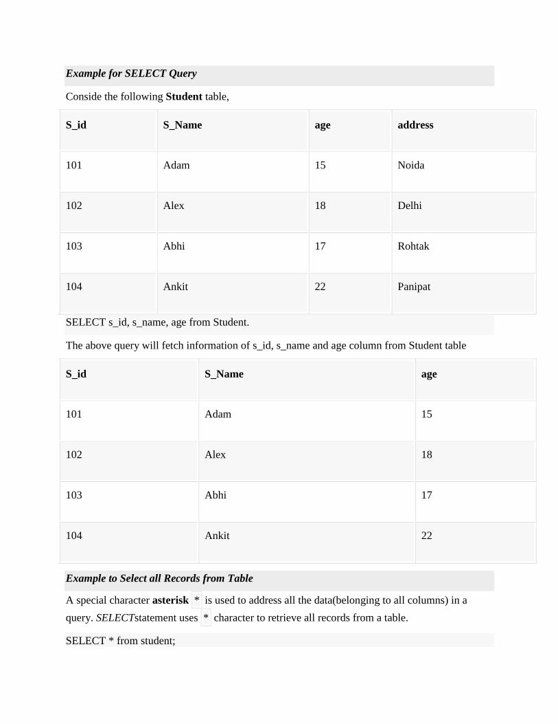
Example for SELECT Query

Conside the following Student table,

S_id S_Name age address

101 Adam 15 Noida

102 Alex 18 Delhi

103 Abhi 17 Rohtak

104 Ankit 22 Panipat

SELECT s_id, s_name, age from Student.

The above query will fetch information of s_id, s_name and age column from Student table

S_id S_Name age

101 Adam 15

102 Alex 18

103 Abhi 17

104 Ankit 22

Example to Select all Records from Table

A special character asterisk * is used to address all the data(belonging to all columns) in a

query. SELECTstatement uses * character to retrieve all records from a table.

SELECT * from student;

The above query will show all the records of Student table, that means it will show complete

Student table as result.

S_id S_Name age address

101 Adam 15 Noida

102 Alex 18 Delhi

103 Abhi 17 Rohtak

104 Ankit 22 Panipat

Example to Select particular Record based on Condition

SELECT * from Student WHERE s_name = 'Abhi';

103 Abhi 17 Rohtak

Example to Perform Simple Calculations using Select Query

Conside the following Employee table.

eid Name age salary

101 Adam 26 5000

102 Ricky 42 8000

103 Abhi 22 10000

104 Rohan 35 5000

SELECT eid, name, salary+3000 from Employee;

The above command will display a new column in the result, showing 3000 added into existing

salaries of the employees.

eid Name salary+3000

101 Adam 8000

102 Ricky 11000

103 Abhi 13000

104 Rohan 8000

Like clause

Like clause is used as condition in SQL query. Like clause compares data with an expression

using wildcard operators. It is used to find similar data from the table.

Wildcard operators

There are two wildcard operators that are used in like clause.

Percent sign % : represents zero, one or more than one character.

Underscore sign _ : represents only one character.

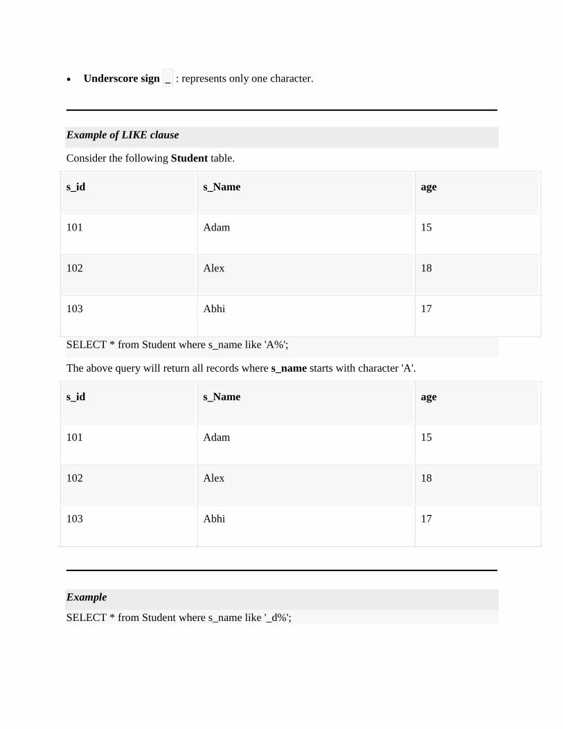
Example of LIKE clause

Consider the following Student table.

s_id s_Name age

101 Adam 15

102 Alex 18

103 Abhi 17

SELECT * from Student where s_name like 'A%';

The above query will return all records where s_name starts with character 'A'.

s_id s_Name age

101 Adam 15

102 Alex 18

103 Abhi 17

Example

SELECT * from Student where s_name like '_d%';

The above query will return all records from Student table where s_name contain 'd' as second

character.

s_id s_Name age

101 Adam 15

Example

SELECT * from Student where s_name like '%x';

The above query will return all records from Student table where s_name contain 'x' as last

character.

s_id s_Name age

102 Alex 18

Order By Clause

Order by clause is used with Select statement for arranging retrieved data in sorted order.

The Order byclause by default sort data in ascending order. To sort data in descending

order DESC keyword is used withOrder by clause.

Syntax of Order By

SELECT column-list|* from table-name order by asc|desc;

Example using Order by

Consider the following Emp table,

eid name age salary

401 Anu 22 9000

402 Shane 29 8000

403 Rohan 34 6000

404 Scott 44 10000

405 Tiger 35 8000

SELECT * from Emp order by salary;

The above query will return result in ascending order of the salary.

eid name age salary

403 Rohan 34 6000

402 Shane 29 8000

405 Tiger 35 8000

401 Anu 22 9000

404 Scott 44 10000

Example of Order by DESC

Consider the Emp table described above,

SELECT * from Emp order by salary DESC;

The above query will return result in descending order of the salary.

eid name age salary

404 Scott 44 10000

401 Anu 22 9000

405 Tiger 35 8000

402 Shane 29 8000

403 Rohan 34 6000

Group By Clause

Group by clause is used to group the results of a SELECT query based on one or more columns.

It is also used with SQL functions to group the result from one or more tables.

Syntax for using Group by in a statement.

SELECT column_name, function(column_name)

FROM table_name

WHERE condition

GROUP BY column_name

Example of Group by in a Statement

Consider the following Emp table.

eid name age salary

401 Anu 22 9000

402 Shane 29 8000

403 Rohan 34 6000

404 Scott 44 9000

405 Tiger 35 8000

Here we want to find name and age of employees grouped by their salaries

SQL query for the above requirement will be,

SELECT name, age

from Emp group by salary

Result will be,

name age

Rohan 34

shane 29

anu 22

Example of Group by in a Statement with WHERE clause

Consider the following Emp table

eid name age salary

401 Anu 22 9000

402 Shane 29 8000

403 Rohan 34 6000

404 Scott 44 9000

405 Tiger 35 8000

SQL query will be,

select name, salary

from Emp

where age > 25

group by salary

Result will be.

name salary

Rohan 6000

Shane 8000

Scott 9000

You must remember that Group By clause will always come at the end, just like the Order by

clause.

HAVING Clause

having clause is used with SQL Queries to give more precise condition for a statement. It is used

to mention condition in Group based SQL functions, just like WHERE clause.

Syntax for having will be,

select column_name, function(column_name)

FROM table_name

WHERE column_name condition

GROUP BY column_name

HAVING function(column_name) condition

Example of HAVING Statement

Consider the following Sale table.

oid order_name previous_balance customer

11 ord1 2000 Alex

12 ord2 1000 Adam

13 ord3 2000 Abhi

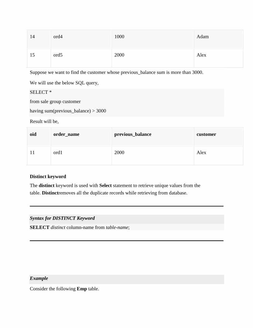
14 ord4 1000 Adam

15 ord5 2000 Alex

Suppose we want to find the customer whose previous_balance sum is more than 3000.

We will use the below SQL query,

SELECT *

from sale group customer

having sum(previous_balance) > 3000

Result will be,

oid order_name previous_balance customer

11 ord1 2000 Alex

Distinct keyword

The distinct keyword is used with Select statement to retrieve unique values from the

table. Distinctremoves all the duplicate records while retrieving from database.

Syntax for DISTINCT Keyword

SELECT distinct column-name from table-name;

Example

Consider the following Emp table.

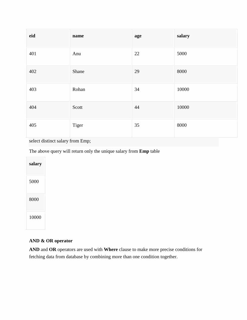
eid name age salary

401 Anu 22 5000

402 Shane 29 8000

403 Rohan 34 10000

404 Scott 44 10000

405 Tiger 35 8000

select distinct salary from Emp;

The above query will return only the unique salary from Emp table

salary

5000

8000

10000

AND & OR operator

AND and OR operators are used with Where clause to make more precise conditions for

fetching data from database by combining more than one condition together.

AND operator

AND operator is used to set multiple conditions with Where clause.

Example of AND

Consider the following Emp table

eid name age salary

401 Anu 22 5000

402 Shane 29 8000

403 Rohan 34 12000

404 Scott 44 10000

405 Tiger 35 9000

SELECT * from Emp WHERE salary < 10000 AND age > 25

The above query will return records where salary is less than 10000 and age greater than 25.

eid name age salary

402 Shane 29 8000

405 Tiger 35 9000

OR operator

OR operator is also used to combine multiple conditions with Where clause. The only difference

between AND and OR is their behaviour. When we use AND to combine two or more than two

conditions, records satisfying all the condition will be in the result. But in case of OR, atleast one

condition from the conditions specified must be satisfied by any record to be in the result.

Example of OR

Consider the following Emp table

eid name age salary

401 Anu 22 5000

402 Shane 29 8000

403 Rohan 34 12000

404 Scott 44 10000

405 Tiger 35 9000

SELECT * from Emp WHERE salary > 10000 OR age > 25

The above query will return records where either salary is greater than 10000 or age greater than

25.

402 Shane 29 8000

403 Rohan 34 12000

404 Scott 44 10000

405 Tiger 35 9000

What is an Operator in SQL?

An operator is a reserved word or a character used primarily in an SQL statement's WHERE

clause to perform operation(s), such as comparisons and arithmetic operations.

Operators are used to specify conditions in an SQL statement and to serve as conjunctions for

multiple conditions in a statement.

Arithmetic operators

Comparison operators

Logical operators

Operators used to negate conditions

SQL Arithmetic Operators:

Assume variable a holds 10 and variable b holds 20, then:

Show Examples

Operator Description Example

+ Addition - Adds values on either side of the operator a + b

will give

30

- Subtraction - Subtracts right hand operand from left hand

operand

a - b will

give -10

* Multiplication - Multiplies values on either side of the

operator

a * b will

give 200

/ Division - Divides left hand operand by right hand operand b / a will

give 2

% Modulus - Divides left hand operand by right hand operand

and returns remainder

b % a

will give

0

SQL Comparison Operators:

Assume variable a holds 10 and variable b holds 20, then:

Show Examples

Operator Description Example

= Checks if the values of two operands are equal or not, if yes

then condition becomes true.

(a = b) is

not true.

!= Checks if the values of two operands are equal or not, if values (a != b)

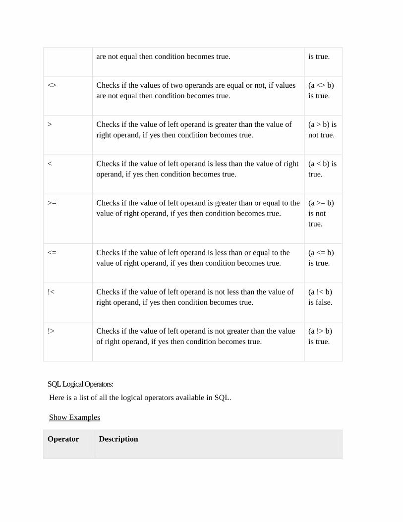
are not equal then condition becomes true. is true.

<> Checks if the values of two operands are equal or not, if values

are not equal then condition becomes true.

(a <> b)

is true.

> Checks if the value of left operand is greater than the value of

right operand, if yes then condition becomes true.

(a > b) is

not true.

< Checks if the value of left operand is less than the value of right

operand, if yes then condition becomes true.

(a < b) is

true.

>= Checks if the value of left operand is greater than or equal to the

value of right operand, if yes then condition becomes true.

(a >= b)

is not

true.

<= Checks if the value of left operand is less than or equal to the

value of right operand, if yes then condition becomes true.

(a <= b)

is true.

!< Checks if the value of left operand is not less than the value of

right operand, if yes then condition becomes true.

(a !< b)

is false.

!> Checks if the value of left operand is not greater than the value

of right operand, if yes then condition becomes true.

(a !> b)

is true.

SQL Logical Operators:

Here is a list of all the logical operators available in SQL.

Show Examples

Operator Description

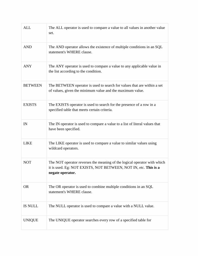
ALL The ALL operator is used to compare a value to all values in another value

set.

AND The AND operator allows the existence of multiple conditions in an SQL

statement's WHERE clause.

ANY The ANY operator is used to compare a value to any applicable value in

the list according to the condition.

BETWEEN The BETWEEN operator is used to search for values that are within a set

of values, given the minimum value and the maximum value.

EXISTS The EXISTS operator is used to search for the presence of a row in a

specified table that meets certain criteria.

IN The IN operator is used to compare a value to a list of literal values that

have been specified.

LIKE The LIKE operator is used to compare a value to similar values using

wildcard operators.

NOT The NOT operator reverses the meaning of the logical operator with which

it is used. Eg: NOT EXISTS, NOT BETWEEN, NOT IN, etc. This is a

negate operator.

OR The OR operator is used to combine multiple conditions in an SQL

statement's WHERE clause.

IS NULL The NULL operator is used to compare a value with a NULL value.

UNIQUE The UNIQUE operator searches every row of a specified table for

uniqueness (no duplicates).

Set Operation in SQL

SQL supports few Set operations to be performed on table data. These are used to get meaningful

results from data, under different special conditions.

Union

UNION is used to combine the results of two or more Select statements. However it will

eliminate duplicate rows from its result set. In case of union, number of columns and datatype

must be same in both the tables.

Example of UNION

The First table,

ID Name

1 abhi

2 adam

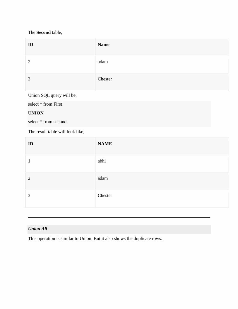
The Second table,

ID Name

2 adam

3 Chester

Union SQL query will be,

select * from First

UNION

select * from second

The result table will look like,

ID NAME

1 abhi

2 adam

3 Chester

Union All

This operation is similar to Union. But it also shows the duplicate rows.

Example of Union All

The First table,

ID NAME

1 abhi

2 adam

The Second table,

ID NAME

2 adam

3 Chester

Union All query will be like,

select * from First

UNION ALL

select * from second

The result table will look like,

ID NAME

1 abhi

2 adam

2 adam

3 Chester

Intersect

Intersect operation is used to combine two SELECT statements, but it only retuns the records

which are common from both SELECT statements. In case of Intersect the number of columns

and datatype must be same. MySQL does not support INTERSECT operator.

Example of Intersect

The First table,

ID NAME

1 abhi

2 adam

The Second table,

ID NAME

2 adam

3 Chester

Intersect query will be,

select * from First

INTERSECT

select * from second

The result table will look like

ID NAME

2 adam

Minus

Minus operation combines result of two Select statements and return only those result which

belongs to first set of result. MySQL does not support INTERSECT operator.

Example of Minus

The First table,

ID NAME

1 abhi

2 adam

The Second table,

ID NAME

2 adam

3 Chester

Minus query will be,

select * from First

MINUS

select * from second

The result table will look like,

ID NAME

1 abhi

The SQL BETWEEN Operator

The BETWEEN operator selects values within a range. The values can be numbers, text, or

dates.

SQL BETWEEN Syntax

SELECT column_name(s)

FROM table_name

WHERE column_name BETWEEN value1 AND value2;

Demo Database

In this tutorial we will use the well-known Northwind sample database.

Below is a selection from the "Products" table:

ProductID ProductName SupplierID CategoryID Unit Price

1 Chais 1 1 10

boxes x

20 bags

18

2 Chang 1 1 24 - 12

oz

bottles

19

3 Aniseed Syrup 1 2 12 - 550

ml

bottles

10

4 Chef Anton's

Cajun Seasoning

1 2 48 - 6

oz jars

22

5 Chef Anton's

Gumbo Mix

1 2 36

boxes

21.35

BETWEEN Operator Example

The following SQL statement selects all products with a price BETWEEN 10 and 20:

Example

SELECT * FROM Products

WHERE Price BETWEEN 10 AND 20;

NOT BETWEEN Operator Example

To display the products outside the range of the previous example, use NOT BETWEEN:

Example

SELECT * FROM Products

WHERE Price NOT BETWEEN 10 AND 20;

BETWEEN Operator with IN Example

The following SQL statement selects all products with a price BETWEEN 10 and 20, but

products with a CategoryID of 1,2, or 3 should not be displayed:

Example

SELECT * FROM Products

WHERE (Price BETWEEN 10 AND 20)

AND NOT CategoryID IN (1,2,3);

BETWEEN Operator with Text Value Example

The following SQL statement selects all products with a ProductName beginning with any of the

letter BETWEEN 'C' and 'M':

Example

SELECT * FROM Products

WHERE ProductName BETWEEN 'C' AND 'M';

NOT BETWEEN Operator with Text Value Example

The following SQL statement selects all products with a ProductName beginning with any of the

letter NOT BETWEEN 'C' and 'M':

Example

SELECT * FROM Products

WHERE ProductName NOT BETWEEN 'C' AND 'M';

Sample Table

Below is a selection from the "Orders" table:

OrderID CustomerID EmployeeID OrderDate ShipperID

10248 90 5 7/4/1996 3

10249 81 6 7/5/1996 1

10250 34 4 7/8/1996 2

10251 84 3 7/9/1996 1

10252 76 4 7/10/1996 2

BETWEEN Operator with Date Value Example

The following SQL statement selects all orders with an OrderDate BETWEEN '04-July-1996'

and '09-July-1996':

Example

SELECT * FROM Orders

WHERE OrderDate BETWEEN #07/04/1996# AND #07/09/1996#;

Pattern matching operators-Like.

The LIKE operator is used in a WHERE clause to search for a specified pattern in a column.

The SQL LIKE Operator

The LIKE operator is used to search for a specified pattern in a column.

SQL LIKE Syntax

SELECT column_name(s)

FROM table_name

WHERE column_name LIKE pattern;

Demo Database

In this tutorial we will use the well-known Northwind sample database.

Below is a selection from the "Customers" table:

CustomerI

D

CustomerNam

e

ContactNam

e

Address City PostalCod

e

Countr

y

1

Alfreds

Futterkiste

Maria

Anders

Obere Str.

57

Berlin 12209 German

y

2 Ana Trujillo

Emparedados y

helados

Ana Trujillo Avda. de la

Constitución

2222

Méxic

o D.F.

05021 Mexico

3 Antonio

Moreno

Taquería

Antonio

Moreno

Mataderos

2312

Méxic

o D.F.

05023 Mexico

4

Around the

Horn

Thomas

Hardy

120 Hanover

Sq.

Londo

n

WA1 1DP UK

5 Berglunds

snabbköp

Christina

Berglund

Berguvsväge

n 8

Luleå S-958 22 Sweden

SQL LIKE Operator Examples

The following SQL statement selects all customers with a City starting with the letter "s":

Example

SELECT * FROM Customers

WHERE City LIKE 's%';

Tip: The "%" sign is used to define wildcards (missing letters) both before and after the pattern.

You will learn more about wildcards in the next chapter.

The following SQL statement selects all customers with a City ending with the letter "s":

Example

SELECT * FROM Customers

WHERE City LIKE '%s';

The following SQL statement selects all customers with a Country containing the pattern "land":

Example

SELECT * FROM Customers

WHERE Country LIKE '%land%';

sing the NOT keyword allows you to select records that do NOT match the pattern.

The following SQL statement selects all customers with Country NOT containing the pattern

"land":

Example

SELECT * FROM Customers

WHERE Country NOT LIKE '%land%';

SQL Functions :

SQL - String Functions

SQL string functions are used primarily for string manipulation. The following table details the important

string functions:

Name Description

ASCII() Returns numeric value of left-most character

BIN() Returns a string representation of the argument

BIT_LENGTH() Returns length of argument in bits

CHAR_LENGTH() Returns number of characters in argument

CHAR() Returns the character for each integer passed

CHARACTER_LENGTH() A synonym for CHAR_LENGTH()

CONCAT_WS() Returns concatenate with separator

CONCAT() Returns concatenated string

CONV() Converts numbers between different number bases

ELT() Returns string at index number

EXPORT_SET()

Returns a string such that for every bit set in the value bits,

you get an on string and for every unset bit, you get an off

string

FIELD()

Returns the index (position) of the first argument in the

subsequent arguments

FIND_IN_SET()

Returns the index position of the first argument within the

second argument

FORMAT()

Returns a number formatted to specified number of decimal

places

HEX() Returns a string representation of a hex value

INSERT()

Inserts a substring at the specified position up to the specified

number of characters

INSTR() Returns the index of the first occurrence of substring

LCASE() Synonym for LOWER()

LEFT() Returns the leftmost number of characters as specified

LENGTH() Returns the length of a string in bytes

LOAD_FILE() Loads the named file

LOCATE() Returns the position of the first occurrence of substring

LOWER() Returns the argument in lowercase

LPAD()

Returns the string argument, left-padded with the specified

string

LTRIM() Removes leading spaces

MAKE_SET()

Returns a set of comma-separated strings that have the

corresponding bit in bits set

MID() Returns a substring starting from the specified position

OCT() Returns a string representation of the octal argument

OCTET_LENGTH() A synonym for LENGTH()

ORD()

If the leftmost character of the argument is a multi-byte

character, returns the code for that character

POSITION() A synonym for LOCATE()

QUOTE() Escapes the argument for use in an SQL statement

REGEXP Pattern matching using regular expressions

REPEAT() Repeats a string the specified number of times

REPLACE() Replaces occurrences of a specified string

REVERSE() Reverses the characters in a string

RIGHT() Returns the specified rightmost number of characters

RPAD() Appends string the specified number of times

RTRIM() Removes trailing spaces

SOUNDEX() Returns a soundex string

SOUNDS LIKE Compares sounds

SPACE() Returns a string of the specified number of spaces

STRCMP() Compares two strings

SUBSTRING_INDEX()

Returns a substring from a string before the specified number

of occurrences of the delimiter

SUBSTRING(), SUBSTR() Returns the substring as specified

TRIM() Removes leading and trailing spaces

UCASE() Synonym for UPPER()

UNHEX() Converts each pair of hexadecimal digits to a character

UPPER() Converts to uppercase

SQL arithmetic functions are :

Functions Description

abs() This SQL ABS() returns the absolute value of a number passed as argument.

ceil() This SQL CEIL() will rounded up any positive or negative decimal value within

the function upwards.

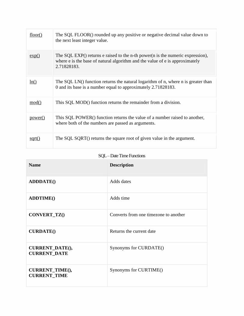
floor() The SQL FLOOR() rounded up any positive or negative decimal value down to

the next least integer value.

exp() The SQL EXP() returns e raised to the n-th power(n is the numeric expression),

where e is the base of natural algorithm and the value of e is approximately

2.71828183.

ln() The SQL LN() function returns the natural logarithm of n, where n is greater than

0 and its base is a number equal to approximately 2.71828183.

mod() This SQL MOD() function returns the remainder from a division.

power() This SQL POWER() function returns the value of a number raised to another,

where both of the numbers are passed as arguments.

sqrt() The SQL SQRT() returns the square root of given value in the argument.

SQL – Date Time Functions

Name Description

ADDDATE() Adds dates

ADDTIME() Adds time

CONVERT_TZ() Converts from one timezone to another

CURDATE() Returns the current date

CURRENT_DATE(),

CURRENT_DATE

Synonyms for CURDATE()

CURRENT_TIME(),

CURRENT_TIME

Synonyms for CURTIME()

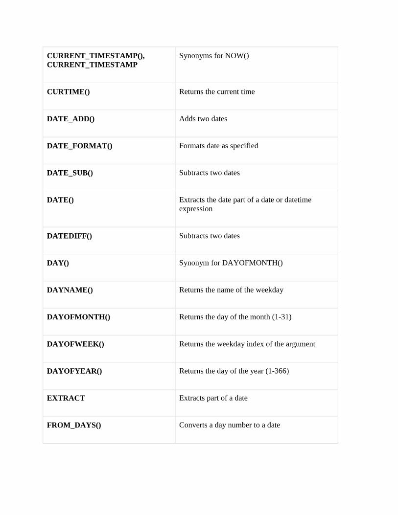
CURRENT_TIMESTAMP(),

CURRENT_TIMESTAMP

Synonyms for NOW()

CURTIME() Returns the current time

DATE_ADD() Adds two dates

DATE_FORMAT() Formats date as specified

DATE_SUB() Subtracts two dates

DATE() Extracts the date part of a date or datetime

expression

DATEDIFF() Subtracts two dates

DAY() Synonym for DAYOFMONTH()

DAYNAME() Returns the name of the weekday

DAYOFMONTH() Returns the day of the month (1-31)

DAYOFWEEK() Returns the weekday index of the argument

DAYOFYEAR() Returns the day of the year (1-366)

EXTRACT Extracts part of a date

FROM_DAYS() Converts a day number to a date

FROM_UNIXTIME() Formats date as a UNIX timestamp

HOUR() Extracts the hour

LAST_DAY Returns the last day of the month for the

argument

LOCALTIME(), LOCALTIME Synonym for NOW()

LOCALTIMESTAMP,

LOCALTIMESTAMP()

Synonym for NOW()

MAKEDATE() Creates a date from the year and day of year

MAKETIME MAKETIME()

MICROSECOND() Returns the microseconds from argument

MINUTE() Returns the minute from the argument

MONTH() Return the month from the date passed

MONTHNAME() Returns the name of the month

NOW() Returns the current date and time

PERIOD_ADD() Adds a period to a year-month

PERIOD_DIFF() Returns the number of months between periods

QUARTER() Returns the quarter from a date argument

SEC_TO_TIME() Converts seconds to 'HH:MM:SS' format

SECOND() Returns the second (0-59)

STR_TO_DATE() Converts a string to a date

SUBDATE() When invoked with three arguments a synonym

for DATE_SUB()

SUBTIME() Subtracts times

SYSDATE() Returns the time at which the function executes

TIME_FORMAT() Formats as time

TIME_TO_SEC() Returns the argument converted to seconds

TIME() Extracts the time portion of the expression

passed

TIMEDIFF() Subtracts time

TIMESTAMP() With a single argument, this function returns the

date or datetime expression. With two

arguments, the sum of the arguments

TIMESTAMPADD() Adds an interval to a datetime expression

TIMESTAMPDIFF() Subtracts an interval from a datetime expression

TO_DAYS() Returns the date argument converted to days

UNIX_TIMESTAMP() Returns a UNIX timestamp

UTC_DATE() Returns the current UTC date

UTC_TIME() Returns the current UTC time

UTC_TIMESTAMP() Returns the current UTC date and time

WEEK() Returns the week number

WEEKDAY() Returns the weekday index

WEEKOFYEAR() Returns the calendar week of the date (1-53)

YEAR() Returns the year

YEARWEEK() Returns the year and week

SQL Aggregate Functions

SQL aggregate functions return a single value, calculated from values in a column.

Useful aggregate functions:

AVG() - Returns the average value

COUNT() - Returns the number of rows

FIRST() - Returns the first value

LAST() - Returns the last value

MAX() - Returns the largest value

MIN() - Returns the smallest value

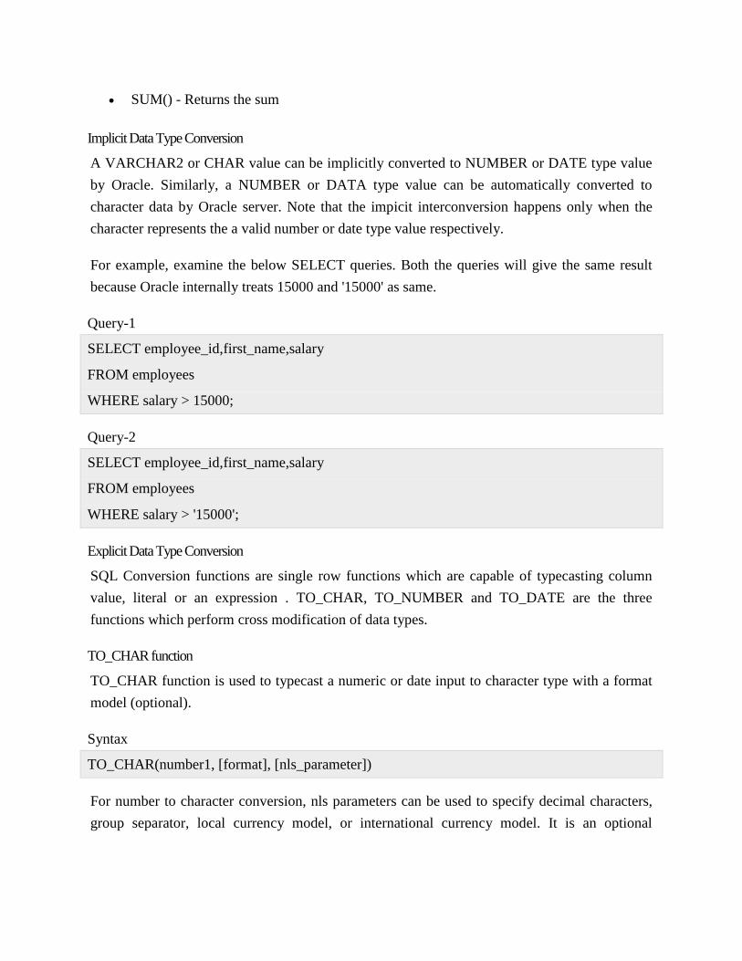
SUM() - Returns the sum

Implicit Data Type Conversion

A VARCHAR2 or CHAR value can be implicitly converted to NUMBER or DATE type value

by Oracle. Similarly, a NUMBER or DATA type value can be automatically converted to

character data by Oracle server. Note that the impicit interconversion happens only when the

character represents the a valid number or date type value respectively.

For example, examine the below SELECT queries. Both the queries will give the same result

because Oracle internally treats 15000 and '15000' as same.

Query-1

SELECT employee_id,first_name,salary

FROM employees

WHERE salary > 15000;

Query-2

SELECT employee_id,first_name,salary

FROM employees

WHERE salary > '15000';

Explicit Data Type Conversion

SQL Conversion functions are single row functions which are capable of typecasting column

value, literal or an expression . TO_CHAR, TO_NUMBER and TO_DATE are the three

functions which perform cross modification of data types.

TO_CHAR function

TO_CHAR function is used to typecast a numeric or date input to character type with a format

model (optional).

Syntax

TO_CHAR(number1, [format], [nls_parameter])

For number to character conversion, nls parameters can be used to specify decimal characters,

group separator, local currency model, or international currency model. It is an optional

specification - if not available, session level nls settings will be used. For date to character

conversion, the nls parameter can be used to specify the day and month names, as applicable.

Dates can be formatted in multiple formats after converting to character types using TO_CHAR

function. The TO_CHAR function is used to have Oracle 11g display dates in a particular

format. Format models are case sensitive and must be enclosed within single quotes.

Consider the below SELECT query. The query format the HIRE_DATE and SALARY columns

of EMPLOYEES table using TO_CHAR function.

SELECT first_name,

TO_CHAR (hire_date, 'MONTH DD, YYYY') HIRE_DATE,

TO_CHAR (salary, '$99999.99') Salary

FROM employees

WHERE rownum < 5;

FIRST_NAME HIRE_DATE SALARY

-------------------- ------------------ ----------

Steven JUNE 17, 2003 $24000.00

Neena SEPTEMBER 21, 2005 $17000.00

Lex JANUARY 13, 2001 $17000.00

Alexander JANUARY 03, 2006 $9000.00

The first TO_CHAR is used to convert the hire date to the date format MONTH DD, YYYY i.e.

month spelled out and padded with spaces, followed by the two-digit day of the month, and then

the four-digit year. If you prefer displaying the month name in mixed case (that is,

"December"), simply use this case in the format argument: ('Month DD, YYYY').

The second TO_CHAR function in Figure 10-39 is used to format the SALARY to display the

currency sign and two decimal positions.

TO_NUMBER function

The TO_NUMBER function converts a character value to a numeric datatype. If the string

being converted contains nonnumeric characters, the function returns an error.

Syntax

TO_NUMBER (string1, [format], [nls_parameter])

The SELECT queries below accept numbers as character inputs and prints them following the

format specifier.

SELECT TO_NUMBER('121.23', '9G999D99')

FROM DUAL

TO_NUMBER('121.23','9G999D99')

------------------------------

121.23

SELECT TO_NUMBER('1210.73', '9999.99')

FROM DUAL;

TO_NUMBER('1210.73','9999.99')

------------------------------

1210.73

TO_DATE function

The function takes character values as input and returns formatted date equivalent of the same.

The TO_DATE function allows users to enter a date in any format, and then it converts the

entry into the default format used by Oracle 11g.

Syntax:

TO_DATE( string1, [ format_mask ], [ nls_language ] )

A format_mask argument consists of a series of elements representing exactly what the data

should look like and must be entered in single quotation marks.

TO_CHAR FUNCTION

DESCRIPTION

The Oracle/PLSQL TO_CHAR function converts a number or date to a string.

SYNTAX

The syntax for the TO_CHAR function in Oracle/PLSQL is:

TO_CHAR( value [, format_mask] [, nls_language] )

Parameters or Arguments

value

A number or date that will be converted to a string.

format_mask

Optional. This is the format that will be used to convert value to a string.

nls_language

Optional. This is the nls language used to convert value to a string.

APPLIES TO

The TO_CHAR function can be used in the following versions of Oracle/PLSQL:

Oracle 12c, Oracle 11g, Oracle 10g, Oracle 9i, Oracle 8i

EXAMPLE

Let's look at some Oracle TO_CHAR function examples and explore how to use the TO_CHAR

function in Oracle/PLSQL.

with Numbers

For example:

The following are number examples for the TO_CHAR function.

TO_CHAR(1210.73, '9999.9')

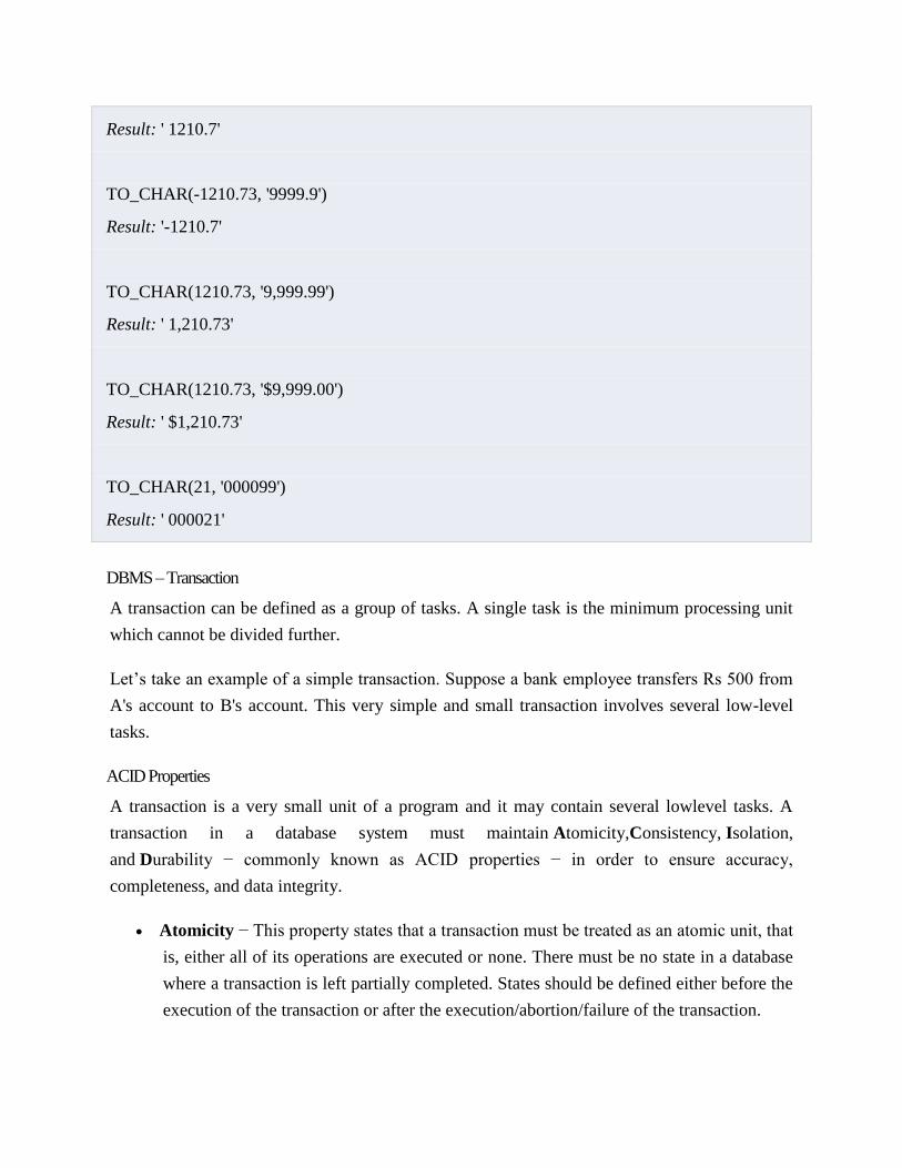
Result: ' 1210.7'

TO_CHAR(-1210.73, '9999.9')

Result: '-1210.7'

TO_CHAR(1210.73, '9,999.99')

Result: ' 1,210.73'

TO_CHAR(1210.73, '$9,999.00')

Result: ' $1,210.73'

TO_CHAR(21, '000099')

Result: ' 000021'

DBMS – Transaction

A transaction can be defined as a group of tasks. A single task is the minimum processing unit

which cannot be divided further.

Let’s take an example of a simple transaction. Suppose a bank employee transfers Rs 500 from

A's account to B's account. This very simple and small transaction involves several low-level

tasks.

ACID Properties

A transaction is a very small unit of a program and it may contain several lowlevel tasks. A

transaction in a database system must maintain Atomicity,Consistency, Isolation,

and Durability − commonly known as ACID properties − in order to ensure accuracy,

completeness, and data integrity.

Atomicity − This property states that a transaction must be treated as an atomic unit, that

is, either all of its operations are executed or none. There must be no state in a database

where a transaction is left partially completed. States should be defined either before the

execution of the transaction or after the execution/abortion/failure of the transaction.

Consistency − The database must remain in a consistent state after any transaction. No

transaction should have any adverse effect on the data residing in the database. If the

database was in a consistent state before the execution of a transaction, it must remain

consistent after the execution of the transaction as well.

Durability − The database should be durable enough to hold all its latest updates even if

the system fails or restarts. If a transaction updates a chunk of data in a database and

commits, then the database will hold the modified data. If a transaction commits but the

system fails before the data could be written on to the disk, then that data will be

updated once the system springs back into action.

Isolation − In a database system where more than one transaction are being executed

simultaneously and in parallel, the property of isolation states that all the transactions

will be carried out and executed as if it is the only transaction in the system. No

transaction will affect the existence of any other transaction.

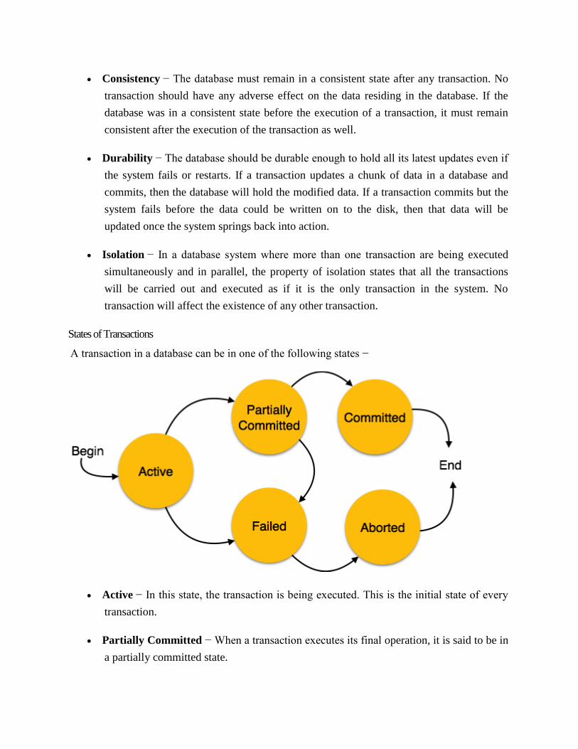
States of Transactions

A transaction in a database can be in one of the following states −

Active − In this state, the transaction is being executed. This is the initial state of every

transaction.

Partially Committed − When a transaction executes its final operation, it is said to be in

a partially committed state.

Failed − A transaction is said to be in a failed state if any of the checks made by the

database recovery system fails. A failed transaction can no longer proceed further.

Aborted − If any of the checks fails and the transaction has reached a failed state, then

the recovery manager rolls back all its write operations on the database to bring the

database back to its original state where it was prior to the execution of the transaction.

Transactions in this state are called aborted. The database recovery module can select

one of the two operations after a transaction aborts −

o Re-start the transaction

o Kill the transaction

Committed − If a transaction executes all its operations successfully, it is said to be

committed. All its effects are now permanently established on the database system.

Concurrent Execution

A schedule is a collection of many transactions which is implemented as a unit. Depending upon

how these transactions are arranged in within a schedule, a schedule can be of two types:

Serial: The transactions are executed one after another, in a non-preemptive manner.

Concurrent: The transactions are executed in a preemptive, time shared method.

In Serial schedule, there is no question of sharing a single data item among many transactions,

because not more than a single transaction is executing at any point of time. However, a serial

schedule is inefficient in the sense that the transactions suffer for having a longer waiting time

and response time, as well as low amount of resource utilization.

In concurrent schedule, CPU time is shared among two or more transactions in order to run them

concurrently. However, this creates the possibility that more than one transaction may need to

access a single data item for read/write purpose and the database could contain inconsistent value

if such accesses are not handled properly. Let us explain with the help of an example.

Let us consider there are two transactions T1 and T2, whose instruction sets are given as

following. T1 is the same as we have seen earlier, while T2 is a new transaction.

T1

Read A;

A = A – 100;

Write A;

Read B;

B = B + 100;

Write B;

T2

Read A;

Temp = A * 0.1;

Read C;

C = C + Temp;

Write C;

T2 is a new transaction which deposits to account C 10% of the amount in account A.

If we prepare a serial schedule, then either T1 will completely finish before T2 can begin, or T2

will completely finish before T1 can begin. However, if we want to create a concurrent schedule,

then some Context Switching need to be made, so that some portion of T1 will be executed, then

some portion of T2 will be executed and so on. For example say we have prepared the following

concurrent schedule.

T1 T2

Read A;

A = A - 100;

Write A;

Read A;

Temp = A * 0.1;

Read C;

C = C + Temp;

Write C;

Read B;

B = B + 100;

Write B;

No problem here. We have made some Context Switching in this Schedule, the first one after

executing the third instruction of T1, and after executing the last statement of T2. T1 first

deducts Rs 100/- from A and writes the new value of Rs 900/- into A. T2 reads the value of A,

calculates the value of Temp to be Rs 90/- and adds the value to C. The remaining part of T1 is

executed and Rs 100/- is added to B.

It is clear that a proper Context Switching is very important in order to maintain the Consistency

and Isolation properties of the transactions. But let us take another example where a wrong

Context Switching can bring about disaster. Consider the following example involving the same

T1 and T2

T1 T2

Read A;

A = A - 100;

Read A;

Temp = A * 0.1;

Read C;

C = C + Temp;

Write C;

Write A;

Read B;

B = B + 100;

Write B;

This schedule is wrong, because we have made the switching at the second instruction of T1. The

result is very confusing. If we consider accounts A and B both containing Rs 1000/- each, then

the result of this schedule should have left Rs 900/- in A, Rs 1100/- in B and add Rs 90 in C (as

C should be increased by 10% of the amount in A). But in this wrong schedule, the Context

Switching is being performed before the new value of Rs 900/- has been updated in A. T2 reads

the old value of A, which is still Rs 1000/-, and deposits Rs 100/- in C. C makes an unjust gain of

Rs 10/- out of nowhere.

In the above example, we detected the error simple by examining the schedule and applying

common sense. But there must be some well formed rules regarding how to arrange instructions

of the transactions to create error free concurrent schedules. This brings us to our next topic, the

concept of Serializability.

Serializability

When multiple transactions are being executed by the operating system in a multiprogramming

environment, there are possibilities that instructions of one transactions are interleaved with

some other transaction.

Schedule − A chronological execution sequence of a transaction is called a schedule. A

schedule can have many transactions in it, each comprising of a number of

instructions/tasks.

Serial Schedule − It is a schedule in which transactions are aligned in such a way that

one transaction is executed first. When the first transaction completes its cycle, then the

next transaction is executed. Transactions are ordered one after the other. This type of

schedule is called a serial schedule, as transactions are executed in a serial manner.

In a multi-transaction environment, serial schedules are considered as a benchmark. The

execution sequence of an instruction in a transaction cannot be changed, but two transactions

can have their instructions executed in a random fashion. This execution does no harm if two

transactions are mutually independent and working on different segments of data; but in case

these two transactions are working on the same data, then the results may vary. This ever-

varying result may bring the database to an inconsistent state.

To resolve this problem, we allow parallel execution of a transaction schedule, if its transactions

are either serializable or have some equivalence relation among them.

DBMS - Deadlock

In a multi-process system, deadlock is an unwanted situation that arises in a shared resource

environment, where a process indefinitely waits for a resource that is held by another process.

For example, assume a set of transactions {T0, T1, T2, ...,Tn}. T0 needs a resource X to complete

its task. Resource X is held by T1, and T1 is waiting for a resource Y, which is held by T2. T2 is

waiting for resource Z, which is held by T0. Thus, all the processes wait for each other to release

resources. In this situation, none of the processes can finish their task. This situation is known

as a deadlock.

Deadlocks are not healthy for a system. In case a system is stuck in a deadlock, the transactions

involved in the deadlock are either rolled back or restarted.

Deadlock Prevention

To prevent any deadlock situation in the system, the DBMS aggressively inspects all the

operations, where transactions are about to execute. The DBMS inspects the operations and

analyzes if they can create a deadlock situation. If it finds that a deadlock situation might occur,

then that transaction is never allowed to be executed.

There are deadlock prevention schemes that use timestamp ordering mechanism of transactions

in order to predetermine a deadlock situation.