introduction to structural equation modeling using stata · introduction to structural equation...
TRANSCRIPT

Introduction to Structural Equation Modeling Using Stata
Chuck HuberStataCorp
University College LondonOctober 16, 2019
Outline
• What is structural equation modeling?
• Structural equation modeling in Stata
• Continuous outcome models using sem
• Multilevel generalized models using gsem
• Demonstrations and Questions

What is Structural Equation Modeling?
• Brief history
• Path diagrams
• Key concepts, jargon and assumptions
• Assessing model fit
• The process of SEM

Brief History of SEM
• Factor analysis had its roots in psychology.– Charles Spearman (1904) is credited with developing the common factor
model. He proposed that correlations between tests of mental abilities could be explained by a common factor representing ability.
– In the 1930s, L. L. Thurston, who was also active in psychometrics, presented work on multiple factor models. He disagreed with the idea of a one general intelligence factor underlying all test scores. He also used an oblique rotation, allowing the factors to be correlated.
– In 1956, T.W. Anderson and H. Rubin discussed testing in factor analysis, and Jöreskog (1969) introduced confirmatory factor analysis and estimation via maximum likelihood estimation, allowing for testing of hypothesis about the number of factors and how they relate to observed variables.

Brief History of SEM• Path analysis and systems of simultaneous equations
developed in genetics, econometrics, and later sociology.– Sewall Wright, a geneticist, is credited with developing path analysis. His
first paper using this method was published in 1918 where he looked at genetic causes related to bone sizes in rabbits. Rather than estimating only the correlation between variables, he created path diagrams to that showed presumed causal paths between variables. He compared what the correlations should be if the variables had the presumed relationships to the observed correlations to evaluate his assumptions.
– In the 1930s, 1940s, and 1950s, many economists including Haavelmo (1943) and Koopmans (1945) worked with systems of simultaneous equations. Economists also introduced a variety of estimation methods and investigated identification issues.
– In the 1960, sociologists including Blalock and Duncan applied path analysis to their research.

Brief History of SEM
• In the early 1970s, these two methods merged.– Hauser and Goldberger (1971) worked on including unobservables into
path models.
– Jöreskog (1973) developed a general model for fitting systems of linear equations and for including latent variables. He also developed the methodology for fitting these models using maximum likelihood estimation and created the program LISREL.
– Keesling (1972) and Wiley (1973) also worked with the general framework combining the two methods.
• Much work has been done since then in to extend these models, to evaluate identification, to test model fit, and more.

What is Structural Equation Modeling?
• Structural equation modeling encompasses a broad array of models from linear regression to measurement models to simultaneous equations.
• Structural equation modeling is not just an estimation method for a particular model.
• Structural equation modeling is a way of thinking, a way of writing, and a way of estimating.
-Stata SEM Manual, pg 2

What is Structural Equation Modeling?
• SEM is a class of statistical techniques that allows us to test hypotheses about relationships among variables.
• SEM may also be referred to as Analysis of Covariance Structures. SEM fits models using the observed covariances and, possibly, means.
• SEM encompasses other statistical methods such as correlation, linear regression, and factor analysis.
• SEM is a multivariate technique that allows us to estimate a system of equations. Variables in these equations may be measured with error. There may be variables in the model that cannot be measured directly.

Structural Equation Models are often drawn as Path Diagrams:

Jargon
• Observed and Latent variables
• Paths and Covariance
• Endogenous and Exogenous variables
• Recursive and Nonrecursive models

Observed and Latent Variables• Observed variables are variables
that are included in our dataset. They are represented by rectangles. The variables satv, satq, and hsgpaare observed variables in this path diagram.
• Latent variables are unobserved variables that we wish we had observed. They can be thought of as the underlying cause of the observed variables. They are represented by ovals. The variable Aptitude is a latent variable in this path diagram.
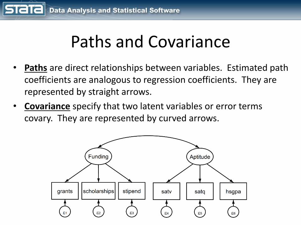
Paths and Covariance
• Paths are direct relationships between variables. Estimated path coefficients are analogous to regression coefficients. They are represented by straight arrows.
• Covariance specify that two latent variables or error terms covary. They are represented by curved arrows.
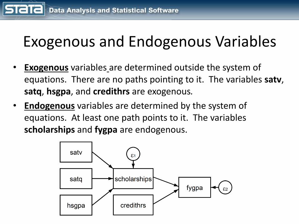
Exogenous and Endogenous Variables
• Exogenous variables are determined outside the system of equations. There are no paths pointing to it. The variables satv, satq, hsgpa, and credithrs are exogenous.
• Endogenous variables are determined by the system of equations. At least one path points to it. The variables scholarships and fygpa are endogenous.

• Observed Exogenous: a variable in a dataset that is treated as exogenous in the model
• Latent Exogenous: an unobserved variable that is treated as exogenous in the model.
• Observed Endogenous: a variable in a dataset that is treated as endogenous in the model
• Latent Endogenous: an unobserved variable that is treated as endogenous in the model.
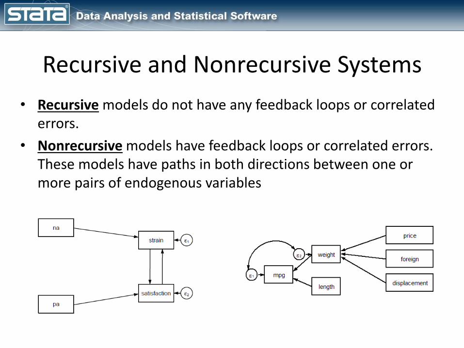
Recursive and Nonrecursive Systems
• Recursive models do not have any feedback loops or correlated errors.
• Nonrecursive models have feedback loops or correlated errors. These models have paths in both directions between one or more pairs of endogenous variables
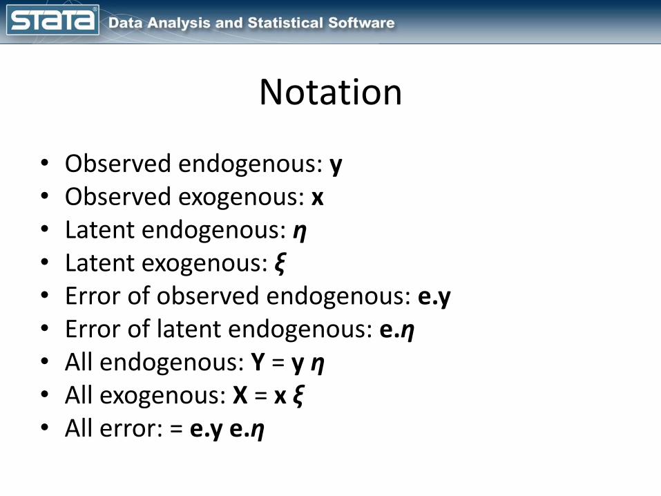
Notation
• Observed endogenous: y• Observed exogenous: x• Latent endogenous: η• Latent exogenous: ξ• Error of observed endogenous: e.y• Error of latent endogenous: e.η• All endogenous: Y = y η• All exogenous: X = x ξ• All error: = e.y e.η

𝑌 = 𝐵𝑌 + Γ𝑋 + 𝛼 + 𝜁
We estimate:• The coefficients B and 𝚪• The intercepts, 𝜶• The means of the exogenous variables 𝜿 = 𝐸(𝑿)• The variances and covariances of the exogenous
variables, 𝜱 = 𝑉𝑎𝑟(𝑿)• The variances and covariances of the errors 𝚿 =𝑉𝑎𝑟(𝜻)

Assumptions
• Large Sample Size
• Multivariate Normality
• Correct Model Specification
Assumptions
• Large Sample Size– ML estimation relies on asymptotics, and large sample
sizes are needed to obtain reliable parameter estimates.
– Different suggestions regarding appropriate sample size have been given by different authors.
– A common rule of thumb is to have a sample size of more than 200, although sometimes 100 is seen as adequate.
– Other authors propose sample sizes relative to the number of parameters being estimated. Ratios of observations to free parameters from 5:1 up to 20:1 have been proposed.
Assumptions
• Multivariate Normality
– The likelihood that is maximized when fitting structural equation models using ML is derived under the assumption that the observed variables follow a multivariate normal distribution.
– The assumption of multivariate normality can often be relaxed, particularly for exogenous variables.
Assumptions
• Correct Model Specification– SEM assumes that no relevant variables are omitted
from any equation in the model.– Omitted variable bias can arise in linear regression if
an independent variable is omitted from the model and the omitted variable is correlated with other independent variables.
– When fitting structural equation models with ML and all equations are fit jointly, errors can occur in equations other than the one with the omitted variable.
What is Structural Equation Modeling?
• Brief history
• Path diagrams
• Key concepts, jargon and assumptions
• Assessing model fit
• The process of SEM
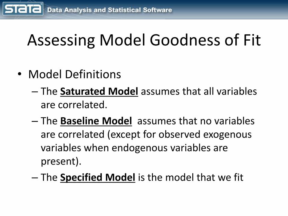
Assessing Model Goodness of Fit
• Model Definitions
– The Saturated Model assumes that all variables are correlated.
– The Baseline Model assumes that no variables are correlated (except for observed exogenous variables when endogenous variables are present).
– The Specified Model is the model that we fit

Likelihood Ratio 𝜒2 (baseline vs saturated models)
𝜒𝑏𝑠2 = 2 𝑙𝑜𝑔 𝐿𝑠 − 𝑙𝑜𝑔𝐿𝑏
where:𝐿𝑏 is the loglikelihood for the baseline model𝐿𝑠 is the loglikelihood for the saturated model𝐿𝑚 is the loglikelihood for the specified model𝑑𝑓𝑏𝑠 = 𝑑𝑓𝑠 − 𝑑𝑓𝑏𝑑𝑓𝑚𝑠 = 𝑑𝑓𝑠 − 𝑑𝑓𝑚
Likelihood Ratio 𝜒2 (specified vs saturated models)
𝜒𝑚𝑠2 = 2 𝑙𝑜𝑔 𝐿𝑠 − 𝑙𝑜𝑔𝐿𝑚

Assessing Model Goodness of Fit• Likelihood Ratio Chi-squared Test (𝜒𝑚𝑠
2 )
• Akaike’s Information Criterion (AIC)
• Swartz’s Bayesian Information Criterion (BIC)
• Coefficient of Determination (𝑅2)
• Root Mean Square Error of Approximation (RMSEA)
• Comparative Fit Index (CFI)
• Tucker-Lewis Index (TLI)
• Standardized Root Mean Square Residual (SRMR)
• Satorra-Bentler adjustment
See also: http://davidakenny.net/cm/fit.htm
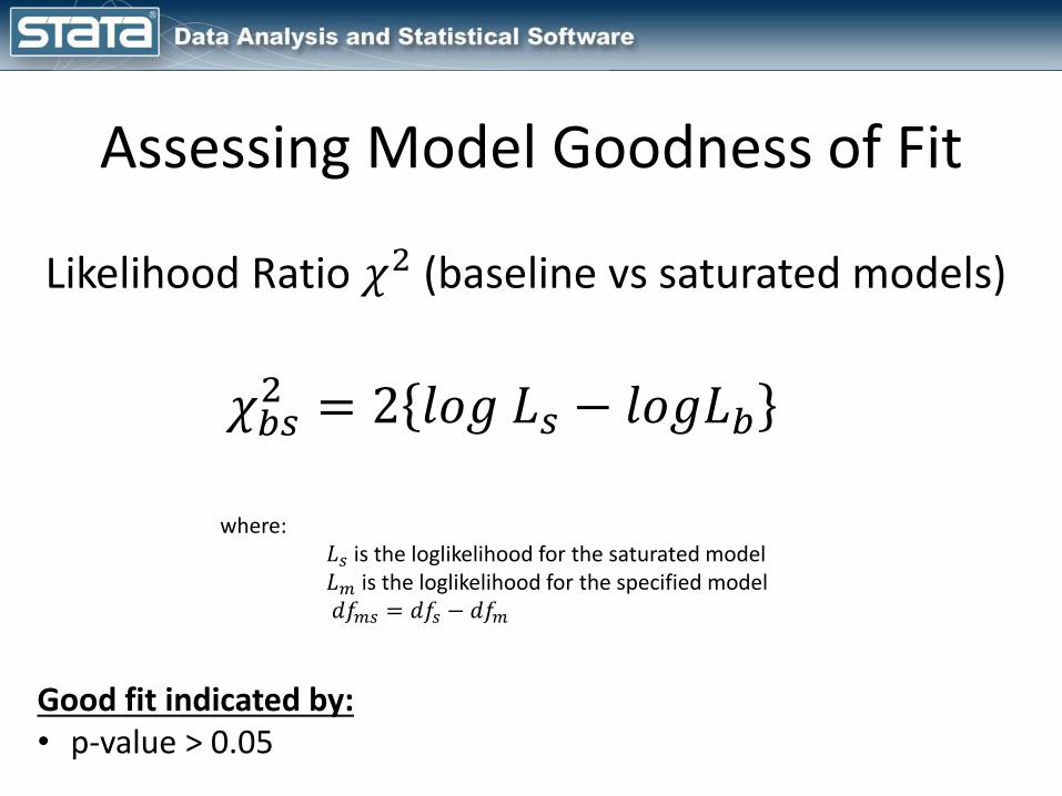
Assessing Model Goodness of Fit
Likelihood Ratio 𝜒2 (baseline vs saturated models)
𝜒𝑏𝑠2 = 2 𝑙𝑜𝑔 𝐿𝑠 − 𝑙𝑜𝑔𝐿𝑏
Good fit indicated by:• p-value > 0.05
where:𝐿𝑠 is the loglikelihood for the saturated model𝐿𝑚 is the loglikelihood for the specified model𝑑𝑓𝑚𝑠 = 𝑑𝑓𝑠 − 𝑑𝑓𝑚
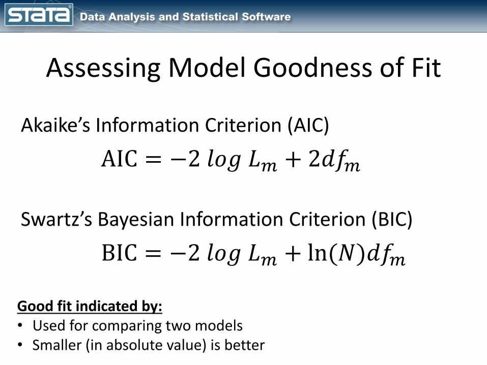
Assessing Model Goodness of Fit
Akaike’s Information Criterion (AIC)
AIC = −2 𝑙𝑜𝑔 𝐿𝑚 + 2𝑑𝑓𝑚
Good fit indicated by:• Used for comparing two models• Smaller (in absolute value) is better
Swartz’s Bayesian Information Criterion (BIC)
BIC = −2 𝑙𝑜𝑔 𝐿𝑚 + ln(𝑁)𝑑𝑓𝑚
Assessing Model Goodness of Fit
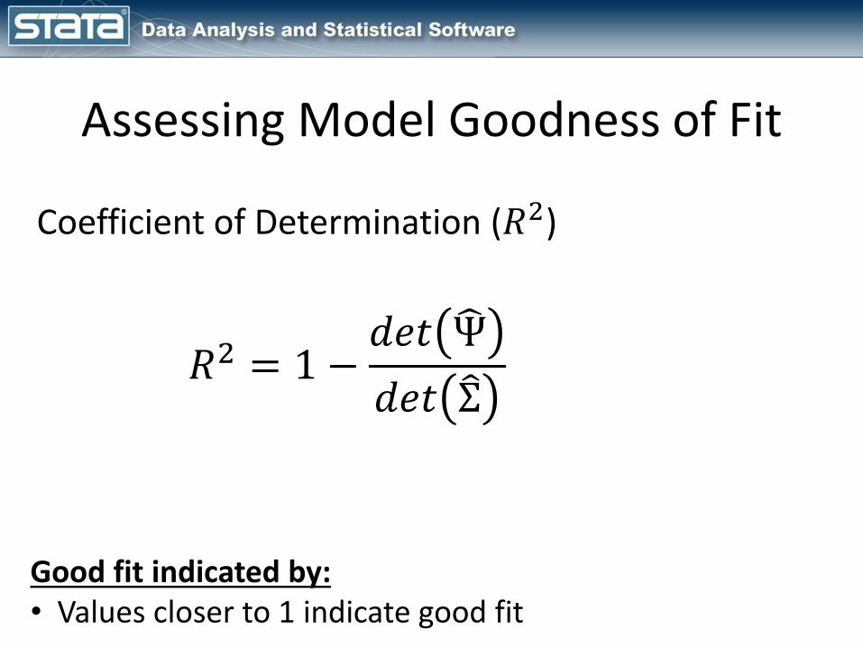
Coefficient of Determination (𝑅2)
𝑅2 = 1 −𝑑𝑒𝑡 Ψ
𝑑𝑒𝑡 Σ
Good fit indicated by:• Values closer to 1 indicate good fit
Assessing Model Goodness of Fit
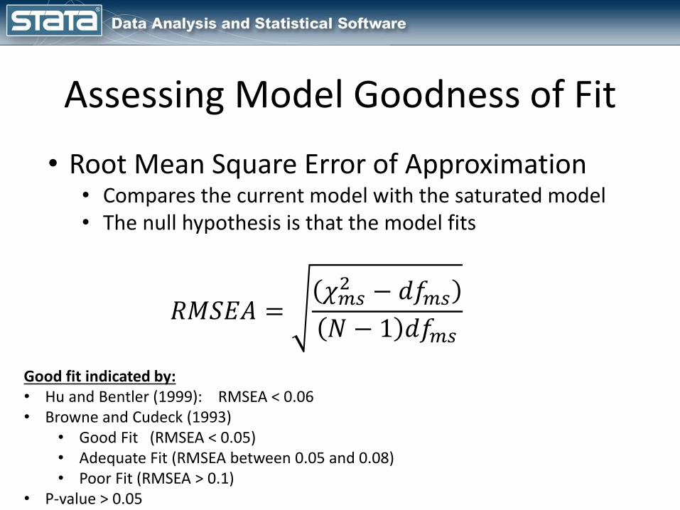
• Root Mean Square Error of Approximation• Compares the current model with the saturated model• The null hypothesis is that the model fits
𝑅𝑀𝑆𝐸𝐴 =𝜒𝑚𝑠2 − 𝑑𝑓𝑚𝑠
𝑁 − 1 𝑑𝑓𝑚𝑠
Good fit indicated by:• Hu and Bentler (1999): RMSEA < 0.06• Browne and Cudeck (1993)
• Good Fit (RMSEA < 0.05) • Adequate Fit (RMSEA between 0.05 and 0.08)• Poor Fit (RMSEA > 0.1)
• P-value > 0.05
Assessing Model Goodness of Fit
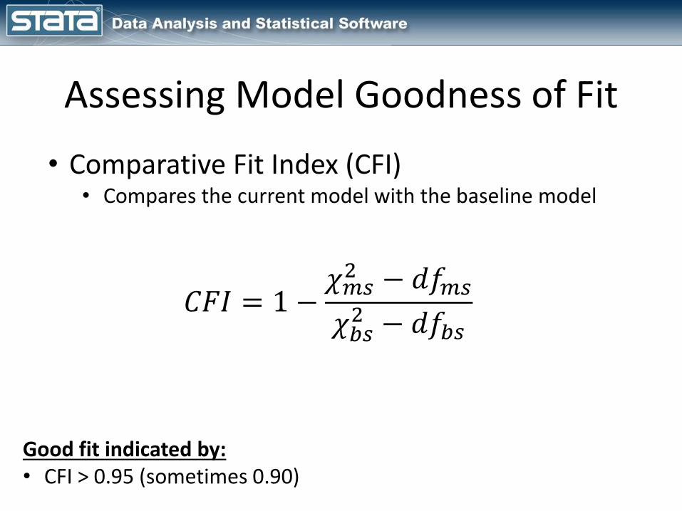
• Comparative Fit Index (CFI)• Compares the current model with the baseline model
𝐶𝐹𝐼 = 1 −𝜒𝑚𝑠2 − 𝑑𝑓𝑚𝑠
𝜒𝑏𝑠2 − 𝑑𝑓𝑏𝑠
Good fit indicated by:• CFI > 0.95 (sometimes 0.90)

Assessing Model Goodness of Fit
Tucker-Lewis Index (TLI)• Compares the current model with the baseline model
𝑇𝐿𝐼 = 1 −Τ𝜒𝑏𝑠
2 𝑑𝑓𝑏𝑠 − Τ𝜒𝑚𝑠2 𝑑𝑓𝑚𝑠
Τ𝜒𝑏𝑠2 𝑑𝑓𝑏𝑠 − 1
Good fit indicated by:• TLI > 0.95
Assessing Model Goodness of Fit
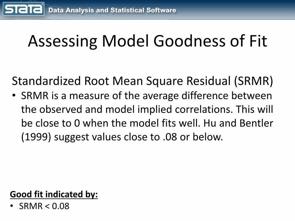
Standardized Root Mean Square Residual (SRMR)• SRMR is a measure of the average difference between
the observed and model implied correlations. This will be close to 0 when the model fits well. Hu and Bentler (1999) suggest values close to .08 or below.
Good fit indicated by:• SRMR < 0.08
The Process of SEM
• Specify the model
• Fit the model
• Evaluate the model
• Modify the model
• Interpret and report the results
Outline
• What is structural equation modeling?
• Structural equation modeling in Stata
• Continuous outcome models using sem
• Multilevel generalized models using gsem
• Demonstrations and Questions
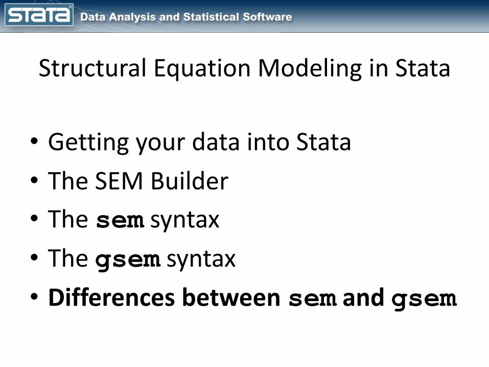
Structural Equation Modeling in Stata
• Getting your data into Stata
• The SEM Builder
• The sem syntax
• The gsem syntax
• Differences between sem and gsem

Getting Data Into Stata
• Can import data using– insheet
– infile
– import excel
• Can open observation level data with use
• Can open summary data with ssd

Getting Data Into Stataclear
ssd init fygpa grants scholarships stipend
ssd set obs 100
ssd set means 2.40 6.43 5.34 0.85
ssd set cov 0.53 \ ///
-0.21 90.99 \ ///
0.72 -8.98 93.29 \ ///
0.06 4.01 0.25 1.54
Note that we will not be able to use gsem with summary data

Getting Data Into Stata. ssd list
Observations = 100
Means:fygpa grants scholarships stipend2.4 6.43 5.34 .85
Variances implicitly defined; they are the diagonal of the covariance matrix.
Covariances:fygpa grants scholarships stipend.53
-.21 90.99.72 -8.98 93.29.06 4.01 .25 1.54

Structural Equation Modeling in Stata
• Getting your data into Stata
• The SEM Builder
• The sem syntax
• The gsem syntax
• Differences between sem and gsem

We can draw path diagrams using Stata’s SEM Builder
Change to generalized SEM
Select (S)
Add Observed Variable (O)
Add Generalized Response Variable (G)
Add Latent Variable (L)
Add Multilevel Latent Variable (U)
Add Path (P)
Add Covariance (C)
Add Measurement Component (M)
Add Observed Variables Set (Shift+O)
Add Latent Variables Set (Shift+L)
Add Regression Component (R)
Add Text (T)
Add Area (A)
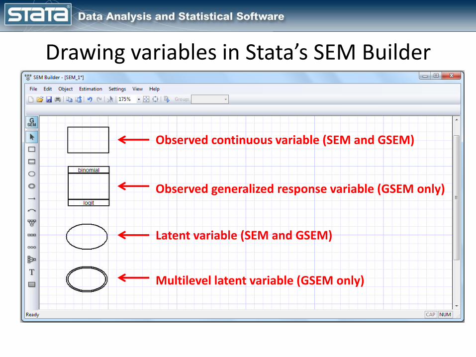
Drawing variables in Stata’s SEM Builder
Observed continuous variable (SEM and GSEM)
Observed generalized response variable (GSEM only)
Latent variable (SEM and GSEM)
Multilevel latent variable (GSEM only)
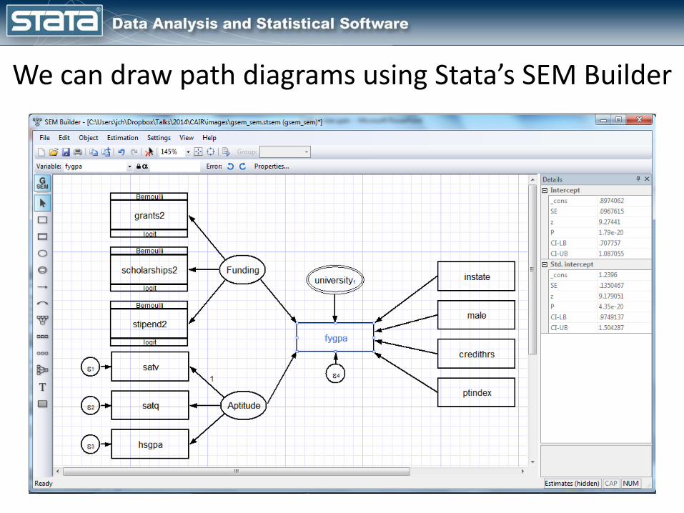
We can draw path diagrams using Stata’s SEM Builder

Structural Equation Modeling in Stata
• Getting your data into Stata
• The SEM Builder
• The sem syntax
• The gsem syntax
• Differences between sem and gsem

sem syntax
sem paths [if] [in] [weight] [, options]
• Paths are specified in parentheses and correspond to the arrows in the path diagrams we saw previously.
• Arrows can point in either direction.
• Paths can be specified individually, or multiple paths can be specified within a single set of parentheses.
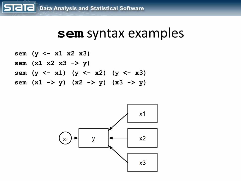
sem syntax examplessem (y <- x1 x2 x3)
sem (x1 x2 x3 -> y)
sem (y <- x1) (y <- x2) (y <- x3)
sem (x1 -> y) (x2 -> y) (x3 -> y)
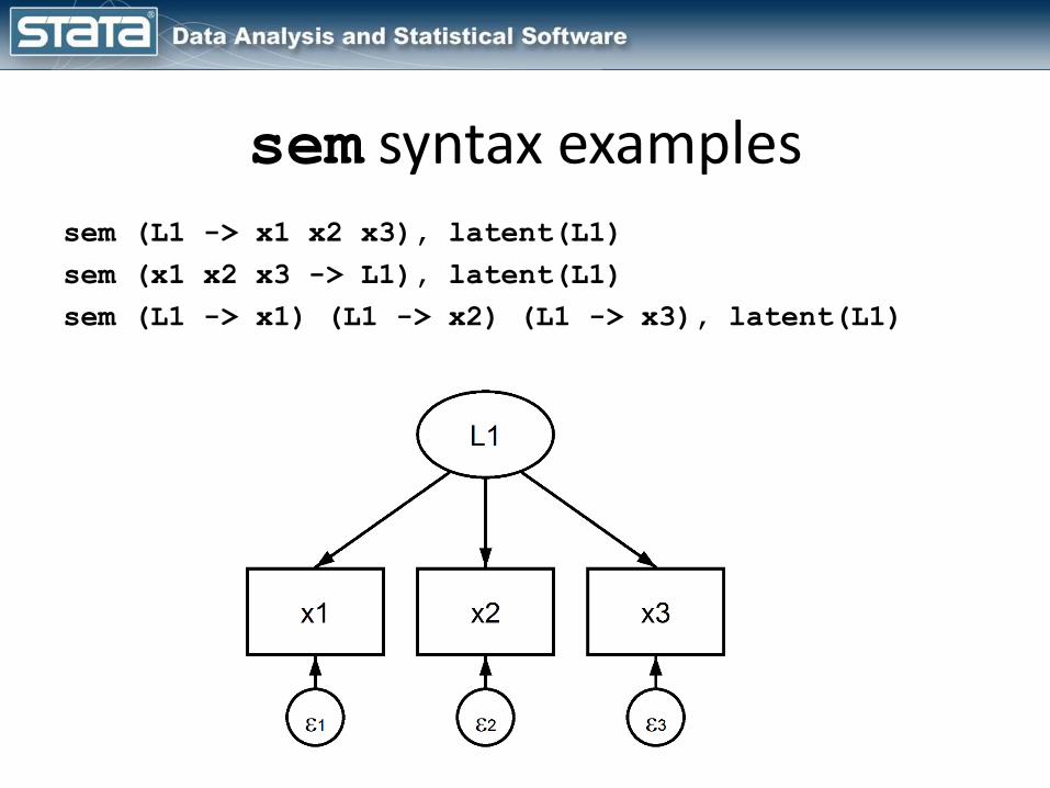
sem syntax examplessem (L1 -> x1 x2 x3), latent(L1)
sem (x1 x2 x3 -> L1), latent(L1)
sem (L1 -> x1) (L1 -> x2) (L1 -> x3), latent(L1)
sem syntax examples
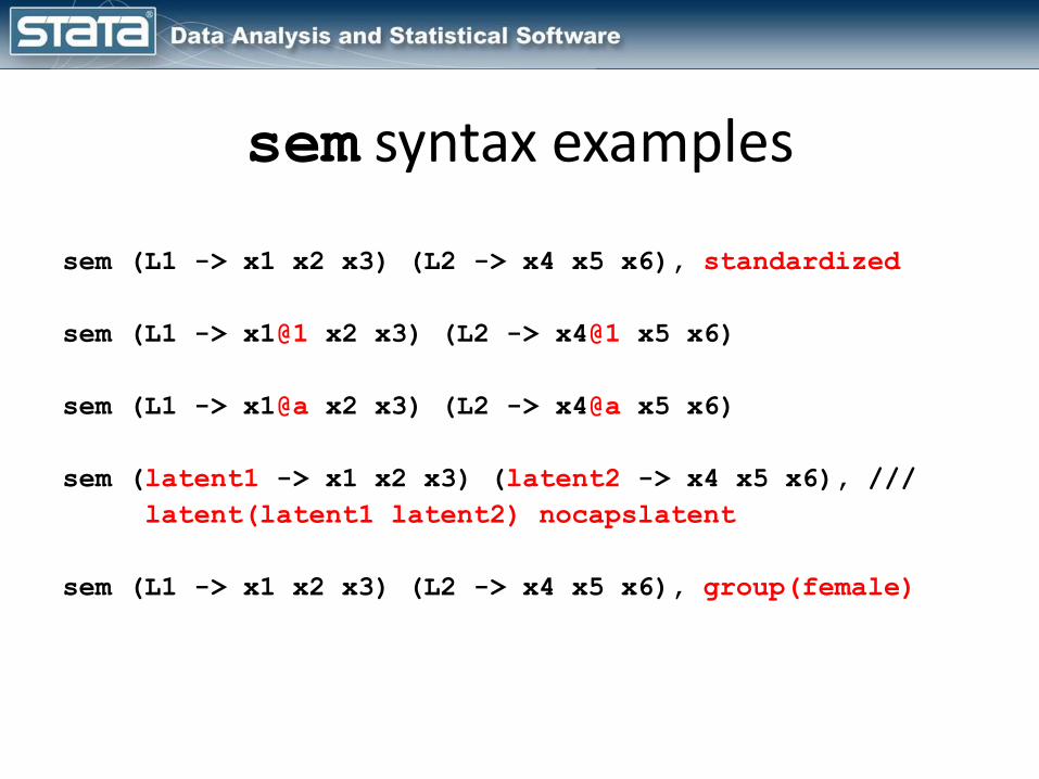
sem (L1 -> x1 x2 x3) (L2 -> x4 x5 x6), standardized
sem (L1 -> x1@1 x2 x3) (L2 -> x4@1 x5 x6)
sem (L1 -> x1@a x2 x3) (L2 -> x4@a x5 x6)
sem (latent1 -> x1 x2 x3) (latent2 -> x4 x5 x6), ///
latent(latent1 latent2) nocapslatent
sem (L1 -> x1 x2 x3) (L2 -> x4 x5 x6), group(female)

Structural Equation Modeling in Stata
• Getting your data into Stata
• The SEM Builder
• The sem syntax
• The gsem syntax
• Differences between sem and gsem
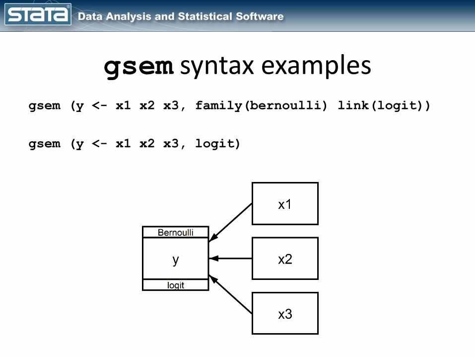
gsem syntax examplesgsem (y <- x1 x2 x3, family(bernoulli) link(logit))
gsem (y <- x1 x2 x3, logit)

Families and Link Functionsidentity log logit probit cloglog
gaussian D X
bernoulli D X X
beta D X X
binomial D X X
ordinal D X X
multinomial D
Poisson D
negative binomial D
exponential D
Weibull D
gamma D
loglogistic D
lognormal D

gsem syntax examples
gsem (y <- x1 x2 x3) ///
(y <- M1[classroom]), ///
latent(M1)
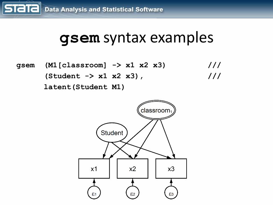
gsem syntax examples
gsem (M1[classroom] -> x1 x2 x3) ///
(Student -> x1 x2 x3), ///
latent(Student M1)

gsem syntax examples
gsem (M1[classroom] -> x1 x2 x3, family(poisson) link(log)) ///
(Student -> x1 x2 x3, family(poisson) link(log)), ///
latent(Student M1)
Structural Equation Modeling in Stata
• Getting your data into Stata
• The SEM Builder
• The sem syntax
• The gsem syntax
• Differences between sem and gsem
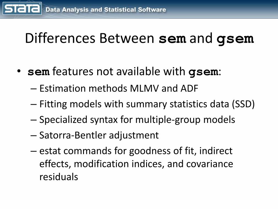
Differences Between sem and gsem
• sem features not available with gsem:
– Estimation methods MLMV and ADF
– Fitting models with summary statistics data (SSD)
– Specialized syntax for multiple-group models
– Satorra-Bentler adjustment
– estat commands for goodness of fit, indirect effects, modification indices, and covariance residuals

Differences Between sem and gsem
• gsem features not available with sem:
– Generalized-linear response variables
– Multilevel models
– Factor-variable notation may be used
– Equation-wise deletion of observations with missing values
– contrast, and pwcompare command may be used after gsem
Differences Between sem and gsem
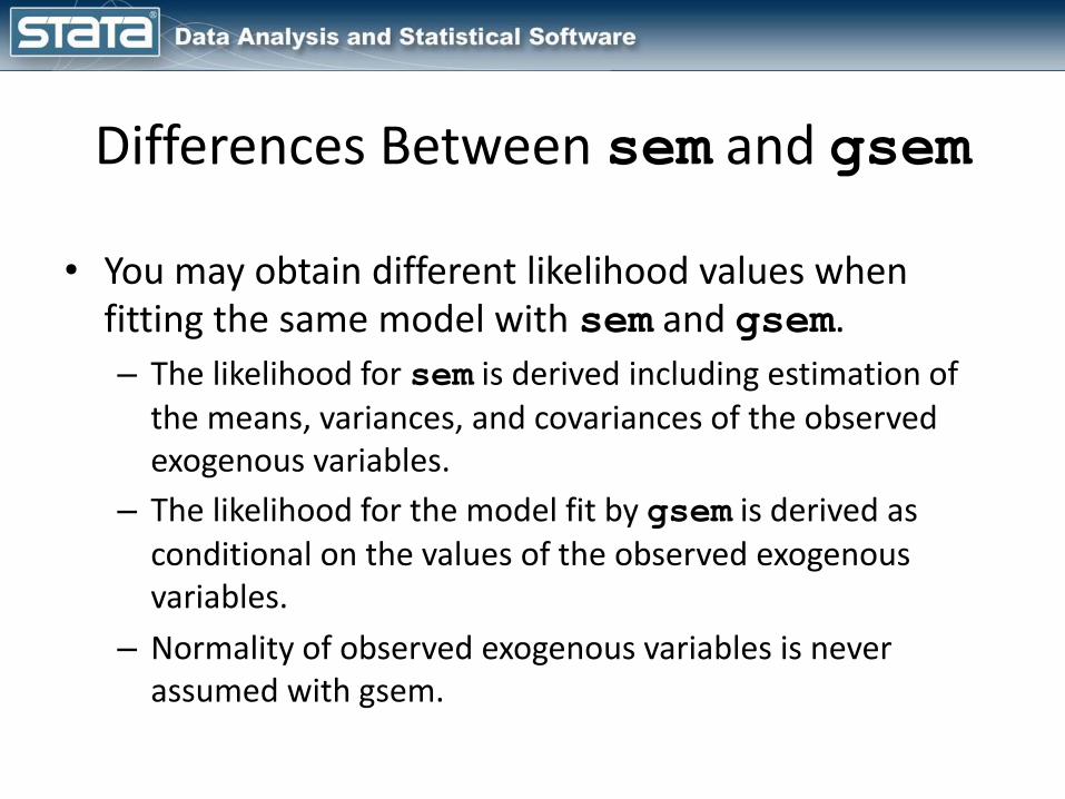
• You may obtain different likelihood values when fitting the same model with sem and gsem.
– The likelihood for sem is derived including estimation of the means, variances, and covariances of the observed exogenous variables.
– The likelihood for the model fit by gsem is derived as conditional on the values of the observed exogenous variables.
– Normality of observed exogenous variables is never assumed with gsem.

Outline
• What is structural equation modeling?
• Structural equation modeling in Stata
• Continuous outcome models using sem
• Multilevel generalized models using gsem
• Demonstrations and Questions

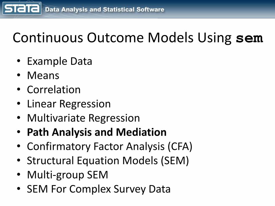
Continuous Outcome Models Using sem
• Example Data• Means• Correlation• Linear Regression• Multivariate Regression• Path Analysis and Mediation• Confirmatory Factor Analysis (CFA)• Structural Equation Models (SEM)• Multi-group SEM• SEM For Complex Survey Data

Example Data. use cair.dta, clear(Example data for the California Association for Institutional Research Workshop)
. describe
storage display valuevariable name type format label variable label----------------------------------------------------------------------------------id int %9.0g Identification Numberuniversity byte %9.0g University IDcollege byte %11.0g college Primary college of majorprivate byte %9.0g private Private or public university?fygpa double %4.2f First-year GPAret_yr1 byte %8.0g YesNo * First-year retentioninstate byte %12.0g instate * In state residencymale byte %8.0g male Malegreek byte %8.0g YesNo * Member of a Greek societywithdrawn double %3.0f * Credits withdrawn or incompletecredithrs double %3.0f * Average number of credits hours
attempted per termptindex double %3.0f * % courses taken in 1st year from
part time facultygrants double %5.1f * Grant money (x1000 dollars)scholarships double %5.1f * Scholarship money (x1000 dollars)stipend double %5.1f * Student work income (x1000 dollars)
* indicated variables have notes----------------------------------------------------------------------------------Sorted by: id

Example Data. summarize
Variable | Obs Mean Std. Dev. Min Max
-------------+--------------------------------------------------------
id | 12958 6479.5 3740.797 1 12958
university | 12958 10.45956 5.735442 1 20
college | 12958 3.052091 1.495687 1 5
private | 12958 .4972218 .5000116 0 1
fygpa | 12875 2.398844 .7274577 0 4
-------------+--------------------------------------------------------
ret_yr1 | 12958 .8924217 .3098591 0 1
instate | 12958 .730977 .4434691 0 1
male | 12958 .4069301 .4912806 0 1
greek | 12958 .2218707 .4155206 0 1
withdrawn | 12947 3.864951 10.26619 0 100
-------------+--------------------------------------------------------
credithrs | 12947 15.62393 1.025208 9 24
ptindex | 12947 44.0851 18.11552 0 100
grants | 12958 6.399958 9.520231 0 49.558
scholarships | 12958 5.319597 9.637058 0 69.288
stipend | 12958 .8426065 1.237821 0 10.79976
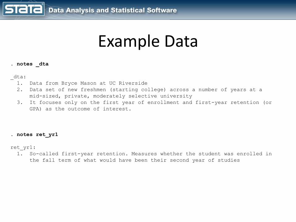
Example Data. notes _dta
_dta:
1. Data from Bryce Mason at UC Riverside
2. Data set of new freshmen (starting college) across a number of years at a
mid-sized, private, moderately selective university
3. It focuses only on the first year of enrollment and first-year retention (or
GPA) as the outcome of interest.
. notes ret_yr1
ret_yr1:
1. So-called first-year retention. Measures whether the student was enrolled in
the fall term of what would have been their second year of studies

Example Data
histogram fygpa, title(Histogram of First Year GPA)

Example Datagraph pie, over(ret_yr1) ///
plabel(_all percent, size(large)) ///
title(Proportion of Students Enrolled For Year 2)

Example Datagraph box fygpa, over(ret_yr1) ///
title(First Year GPA by Enrollment Status for Year 2)

Example Datatwoway (scatter fygpa grants), ///
title(First Year GPA by Grant Money Received)
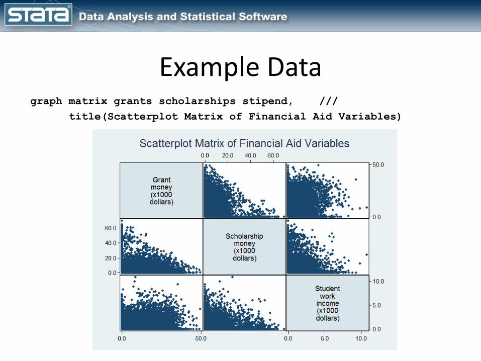
Example Datagraph matrix grants scholarships stipend, ///
title(Scatterplot Matrix of Financial Aid Variables)

Continuous Outcome Models Using sem
• Example Data• Means• Correlation• Linear Regression• Multivariate Regression• Path Analysis and Mediation• Confirmatory Factor Analysis (CFA)• Structural Equation Models (SEM)• Multi-group SEM• SEM For Complex Survey Data
Sample Mean Path Diagram
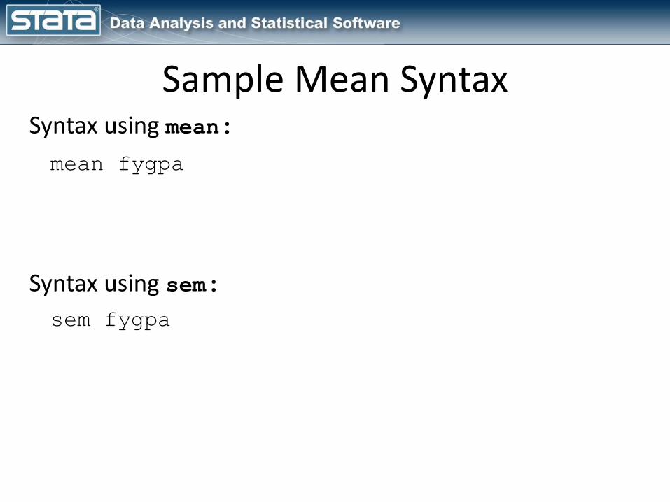
Sample Mean SyntaxSyntax using mean:
Syntax using sem:
mean fygpa
sem fygpa

Sample Mean ResultsResults using means:
Results using sem:
fygpa 2.398844 .0064111 2.386277 2.411411 Mean Std. Err. [95% Conf. Interval]
Mean estimation Number of obs = 12875
LR test of model vs. saturated: chi2(0) = 0.00, Prob > chi2 = . var(fygpa) .5291536 .0065951 .516384 .542239 mean(fygpa) 2.398844 .0064109 374.18 0.000 2.386279 2.411409 Coef. Std. Err. z P>|z| [95% Conf. Interval] OIM

Continuous Outcome Models Using sem
• Example Data• Means• Correlation• Linear Regression• Multivariate Regression• Path Analysis and Mediation• Confirmatory Factor Analysis (CFA)• Structural Equation Models (SEM)• Multi-group SEM• SEM For Complex Survey Data

Correlation Path Diagram
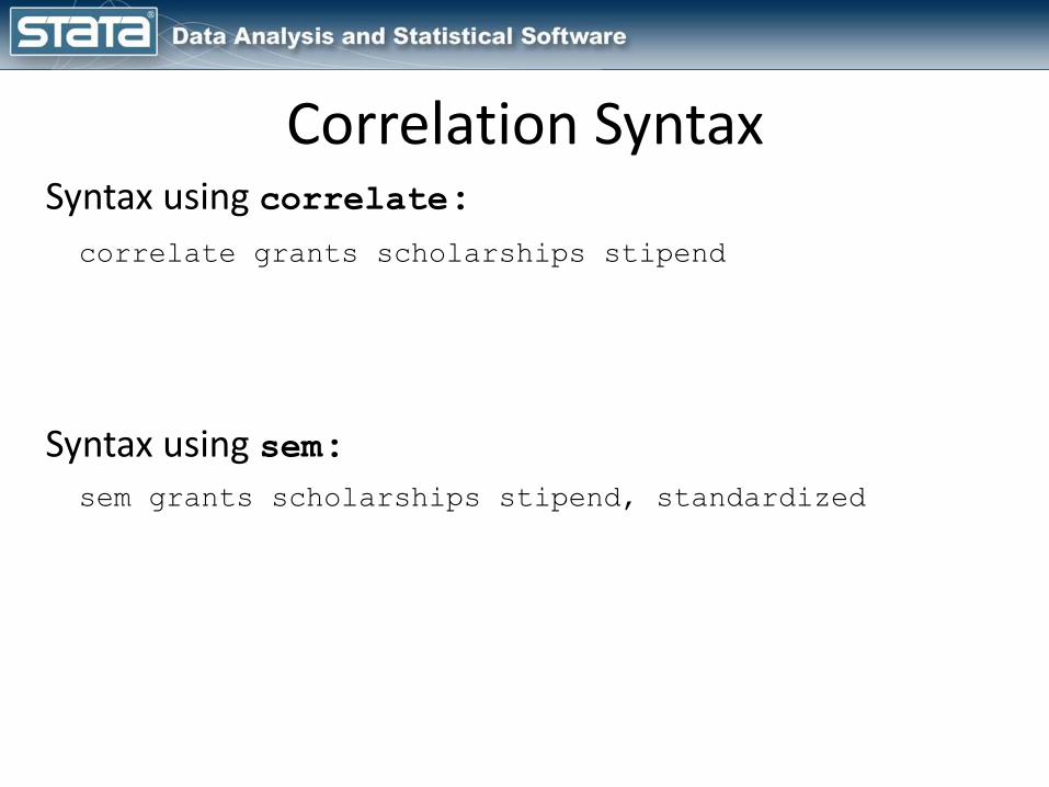
Correlation SyntaxSyntax using correlate:
Syntax using sem:
correlate grants scholarships stipend
sem grants scholarships stipend, standardized

Correlation ResultsResults using correlate:
Results using sem:
stipend 0.3402 0.0225 1.0000scholarships -0.0958 1.0000 grants 1.0000 grants schola~s stipend
LR test of model vs. saturated: chi2(0) = 0.00, Prob > chi2 = . stipend) .0225183 .0087803 2.56 0.010 .0053091 .0397274 cov(scholars~s, stipend) .3402038 .007768 43.80 0.000 .3249787 .3554289 cov(grants, scholarships) -.095848 .0087041 -11.01 0.000 -.1129077 -.0787884 cov(grants, var(stipend) 1 . . .var(scholarsh~s) 1 . . . var(grants) 1 . . . mean(stipend) .680744 .0097496 69.82 0.000 .6616353 .6998528mean(scholars~s) .5520152 .0094303 58.54 0.000 .5335321 .5704982 mean(grants) .6722741 .0097268 69.12 0.000 .6532098 .6913384 Standardized Coef. Std. Err. z P>|z| [95% Conf. Interval] OIM

Continuous Outcome Models Using sem
• Example Data• Means• Correlation• Linear Regression• Multivariate Regression• Path Analysis and Mediation• Confirmatory Factor Analysis (CFA)• Structural Equation Models (SEM)• Multi-group SEM• SEM For Complex Survey Data

Linear Regression Path Diagram
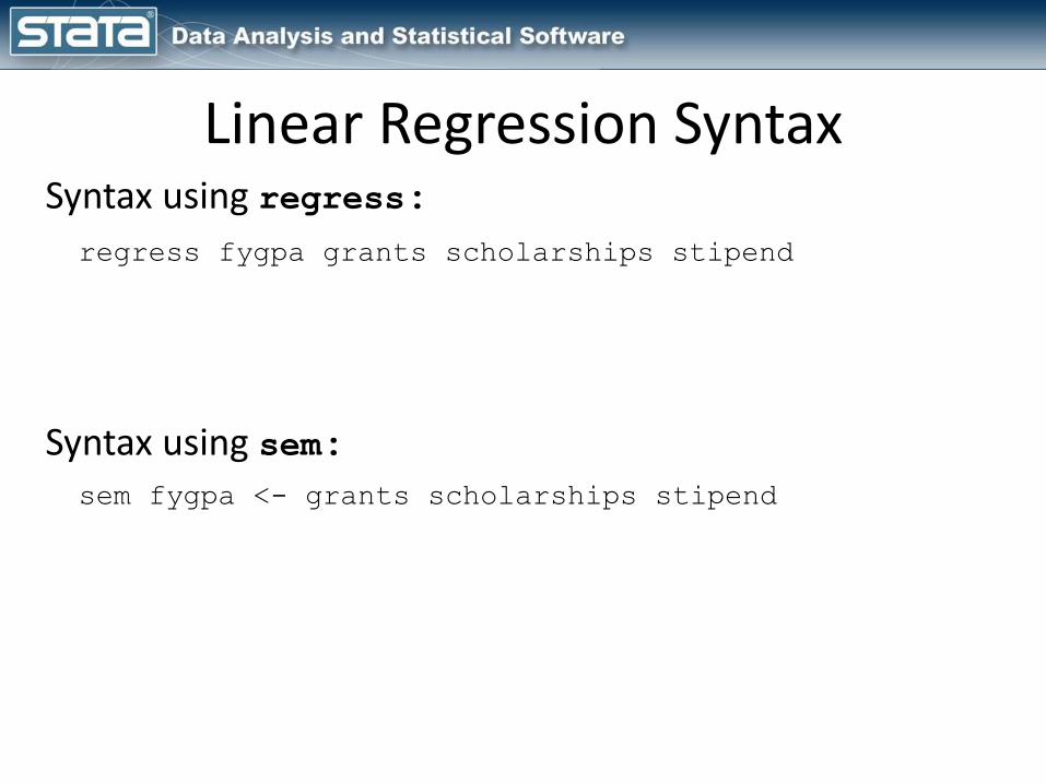
Linear Regression SyntaxSyntax using regress:
Syntax using sem:
regress fygpa grants scholarships stipend
sem fygpa <- grants scholarships stipend

Linear Regression ResultsResults using regress:
Results using sem:
_cons 2.345305 .0090911 257.98 0.000 2.327485 2.363125 stipend .04439 .0054608 8.13 0.000 .0336861 .055094scholarships .0072665 .0006628 10.96 0.000 .0059673 .0085657 grants -.003563 .0007131 -5.00 0.000 -.0049608 -.0021651 fygpa Coef. Std. Err. t P>|t| [95% Conf. Interval]
var(e.fygpa) .5206841 .0064896 .5081189 .5335601 _cons 2.345305 .0090897 258.02 0.000 2.327489 2.36312 stipend .04439 .0054599 8.13 0.000 .0336888 .0550913 scholarships .0072665 .0006627 10.97 0.000 .0059676 .0085653 grants -.003563 .000713 -5.00 0.000 -.0049605 -.0021654 fygpa <- Structural Coef. Std. Err. z P>|z| [95% Conf. Interval] OIM

Continuous Outcome Models Using sem
• Example Data• Means• Correlation• Linear Regression• Multivariate Regression• Path Analysis and Mediation• Confirmatory Factor Analysis (CFA)• Structural Equation Models (SEM)• Multi-group SEM• SEM For Complex Survey Data

Multivariate Regression Path Diagram

Multivariate Regression SyntaxSyntax using mvreg:
Syntax using sem:
mvreg grants scholarships = satv satq hsgpa
sem (grants scholarships <- satv satq hsgpa), ///
cov(e.scholarships*e.grants)
sem (grants <- satv satq hsgpa) ///
(scholarships <- satv satq hsgpa), ///
cov(e.scholarships*e.grants)

Multivariate Regression Results
Results using mvreg:
_cons 4.975286 .1283862 38.75 0.000 4.72363 5.226942 hsgpa -.1293269 .1038093 -1.25 0.213 -.3328086 .0741548 satq .1581007 .1040054 1.52 0.129 -.0457652 .3619666 satv .2711446 .1009657 2.69 0.007 .0732369 .4690524scholarships _cons 6.467567 .1268666 50.98 0.000 6.218889 6.716244 hsgpa .0946835 .1025807 0.92 0.356 -.1063898 .2957568 satq -.0317529 .1027744 -0.31 0.757 -.2332059 .1697001 satv -.0556837 .0997707 -0.56 0.577 -.251249 .1398816grants Coef. Std. Err. t P>|t| [95% Conf. Interval]

Multivariate Regression Results
Results using sem:
e.scholarships) -8.958597 .8151842 -10.99 0.000 -10.55633 -7.360866 cov(e.grants, var(e.scholar~s) 93.1652 1.161168 90.91693 95.46908 var(e.grants) 90.97287 1.133844 88.7775 93.22253 _cons 4.975286 .1283662 38.76 0.000 4.723693 5.226879 hsgpa -.1293269 .1037932 -1.25 0.213 -.3327578 .0741041 satq .1581007 .1039892 1.52 0.128 -.0457144 .3619158 satv .2711446 .10095 2.69 0.007 .0732862 .469003 scholars~s <- _cons 6.467567 .1268469 50.99 0.000 6.218951 6.716182 hsgpa .0946835 .1025647 0.92 0.356 -.1063397 .2957067 satq -.0317529 .1027584 -0.31 0.757 -.2331556 .1696499 satv -.0556837 .0997552 -0.56 0.577 -.2512003 .1398329 grants <- Structural Coef. Std. Err. z P>|z| [95% Conf. Interval] OIM
Continuous Outcome Models Using sem
• Example Data• Means• Correlation• Linear Regression• Multivariate Regression• Path Analysis and Mediation• Confirmatory Factor Analysis (CFA)• Structural Equation Models (SEM)• Multi-group SEM• SEM For Complex Survey Data
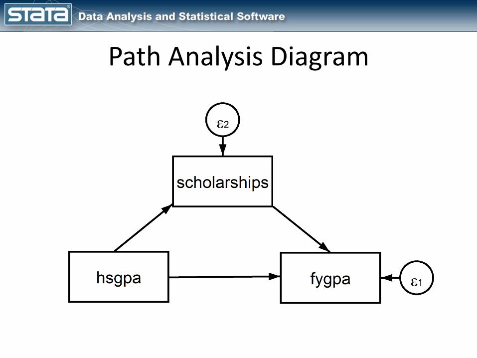
Path Analysis Diagram
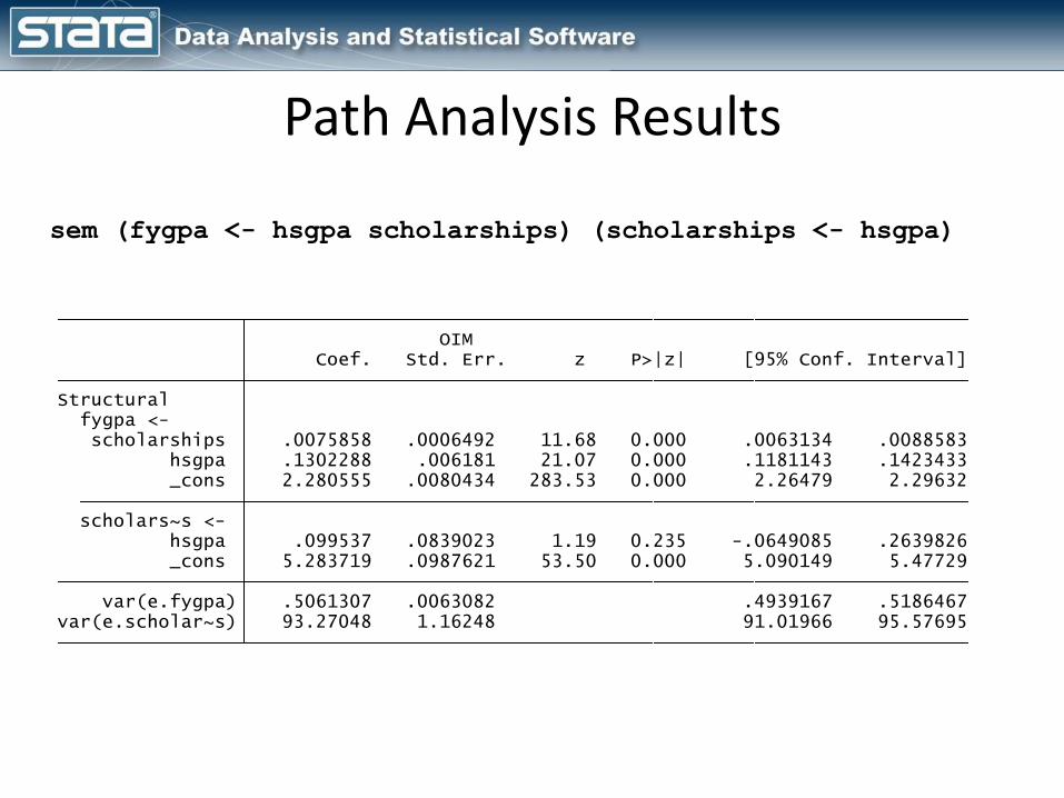
Path Analysis Results
sem (fygpa <- hsgpa scholarships) (scholarships <- hsgpa)
var(e.scholar~s) 93.27048 1.16248 91.01966 95.57695 var(e.fygpa) .5061307 .0063082 .4939167 .5186467 _cons 5.283719 .0987621 53.50 0.000 5.090149 5.47729 hsgpa .099537 .0839023 1.19 0.235 -.0649085 .2639826 scholars~s <- _cons 2.280555 .0080434 283.53 0.000 2.26479 2.29632 hsgpa .1302288 .006181 21.07 0.000 .1181143 .1423433 scholarships .0075858 .0006492 11.68 0.000 .0063134 .0088583 fygpa <- Structural Coef. Std. Err. z P>|z| [95% Conf. Interval] OIM

Mediation Analysis
Total Effect (c) of high school GPA on first year GPA
Indirect Effect (a & b) of high school GPA on first year GPAthrough the mediator scholarships
Direct Effect (c’) of high school GPA on first year GPA
𝑐 = 𝑐′ + 𝑎𝑏

estat teffects, compact
hsgpa .099537 .0839023 1.19 0.235 -.0649085 .2639826 scholars~s <- hsgpa .1309839 .0062133 21.08 0.000 .118806 .1431618 scholarships .0075858 .0006492 11.68 0.000 .0063134 .0088583 fygpa <- Structural Coef. Std. Err. z P>|z| [95% Conf. Interval] OIM Total effects
scholars~s <- hsgpa .0007551 .0006397 1.18 0.238 -.0004988 .0020089 fygpa <- Structural Coef. Std. Err. z P>|z| [95% Conf. Interval] OIM Indirect effects
hsgpa .099537 .0839023 1.19 0.235 -.0649085 .2639826 scholars~s <- hsgpa .1302288 .006181 21.07 0.000 .1181143 .1423433 scholarships .0075858 .0006492 11.68 0.000 .0063134 .0088583 fygpa <- Structural Coef. Std. Err. z P>|z| [95% Conf. Interval] OIM Direct effects

Continuous Outcome Models Using sem
• Example Data• Means• Correlation• Linear Regression• Multivariate Regression• Path Analysis and Mediation• Confirmatory Factor Analysis (CFA)• Structural Equation Models (SEM)• Multi-group SEM• SEM For Complex Survey Data
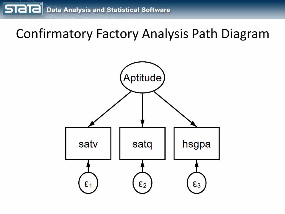
Confirmatory Factory Analysis Path Diagram
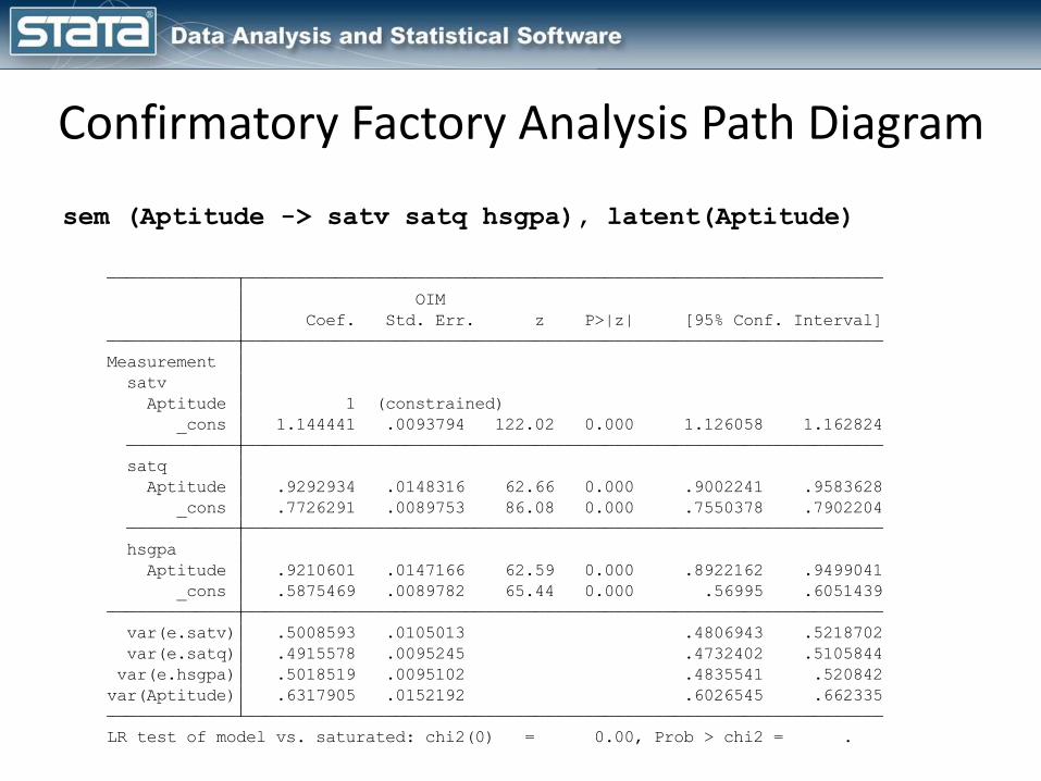
sem (Aptitude -> satv satq hsgpa), latent(Aptitude)
Confirmatory Factory Analysis Path Diagram
LR test of model vs. saturated: chi2(0) = 0.00, Prob > chi2 = .
var(Aptitude) .6317905 .0152192 .6026545 .662335
var(e.hsgpa) .5018519 .0095102 .4835541 .520842
var(e.satq) .4915578 .0095245 .4732402 .5105844
var(e.satv) .5008593 .0105013 .4806943 .5218702
_cons .5875469 .0089782 65.44 0.000 .56995 .6051439
Aptitude .9210601 .0147166 62.59 0.000 .8922162 .9499041
hsgpa
_cons .7726291 .0089753 86.08 0.000 .7550378 .7902204
Aptitude .9292934 .0148316 62.66 0.000 .9002241 .9583628
satq
_cons 1.144441 .0093794 122.02 0.000 1.126058 1.162824
Aptitude 1 (constrained)
satv
Measurement
Coef. Std. Err. z P>|z| [95% Conf. Interval]
OIM

Confirmatory Factory Analysis Path Diagram
sem (Funding -> grants_c@1 scholarships_c stipend_c) ///
(Aptitude -> satv@1 satq hsgpa), ///
latent(Funding Aptitude) ///
cov( Funding*Aptitude)
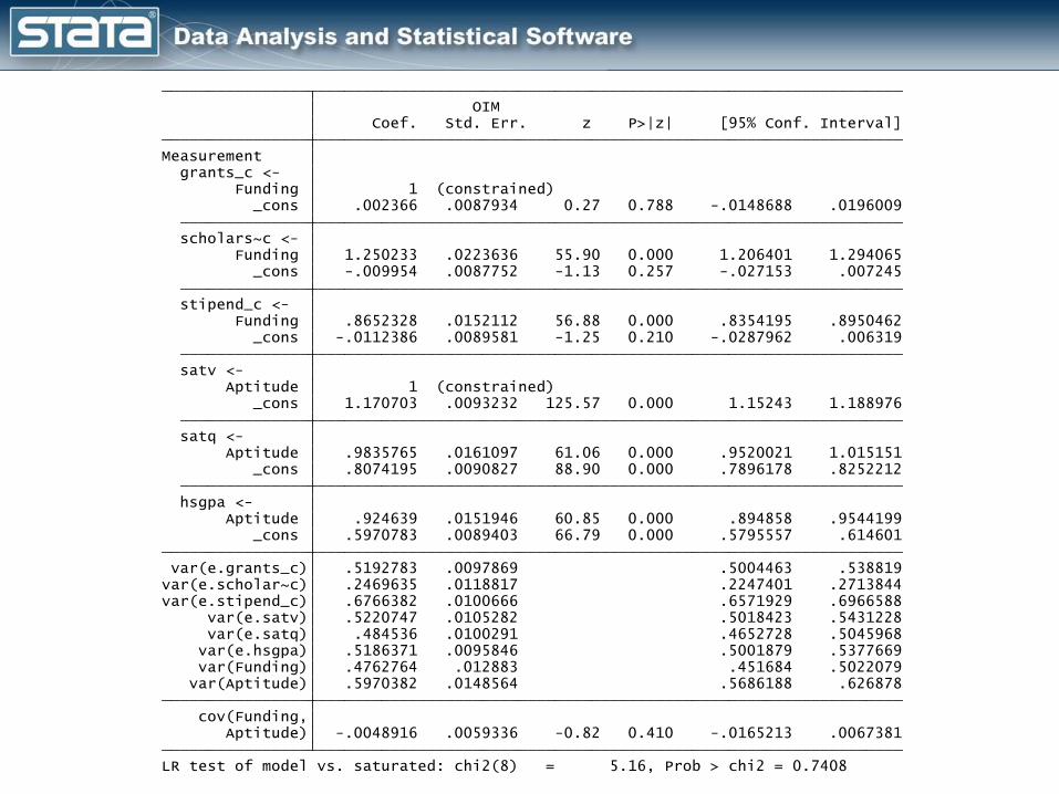
LR test of model vs. saturated: chi2(8) = 5.16, Prob > chi2 = 0.7408 Aptitude) -.0048916 .0059336 -0.82 0.410 -.0165213 .0067381 cov(Funding, var(Aptitude) .5970382 .0148564 .5686188 .626878 var(Funding) .4762764 .012883 .451684 .5022079 var(e.hsgpa) .5186371 .0095846 .5001879 .5377669 var(e.satq) .484536 .0100291 .4652728 .5045968 var(e.satv) .5220747 .0105282 .5018423 .5431228var(e.stipend_c) .6766382 .0100666 .6571929 .6966588var(e.scholar~c) .2469635 .0118817 .2247401 .2713844 var(e.grants_c) .5192783 .0097869 .5004463 .538819 _cons .5970783 .0089403 66.79 0.000 .5795557 .614601 Aptitude .924639 .0151946 60.85 0.000 .894858 .9544199 hsgpa <- _cons .8074195 .0090827 88.90 0.000 .7896178 .8252212 Aptitude .9835765 .0161097 61.06 0.000 .9520021 1.015151 satq <- _cons 1.170703 .0093232 125.57 0.000 1.15243 1.188976 Aptitude 1 (constrained) satv <- _cons -.0112386 .0089581 -1.25 0.210 -.0287962 .006319 Funding .8652328 .0152112 56.88 0.000 .8354195 .8950462 stipend_c <- _cons -.009954 .0087752 -1.13 0.257 -.027153 .007245 Funding 1.250233 .0223636 55.90 0.000 1.206401 1.294065 scholars~c <- _cons .002366 .0087934 0.27 0.788 -.0148688 .0196009 Funding 1 (constrained) grants_c <- Measurement Coef. Std. Err. z P>|z| [95% Conf. Interval] OIM
Continuous Outcome Models Using sem
• Example Data• Means• Correlation• Linear Regression• Multivariate Regression• Path Analysis and Mediation• Confirmatory Factor Analysis (CFA)• Structural Equation Models (SEM)• Multi-group SEM• SEM For Complex Survey Data

Structural Equation Model Path Diagram
sem (Funding -> grants_c@1 scholarships_c stipend_c) ///
(Aptitude -> satv@1 satq hsgpa) ///
(Funding Aptitude -> fygpa), ///
latent(Funding Aptitude)

Structural Equation Model Path Diagram
sem (Funding -> grants_c@1 scholarships_c stipend_c) ///
(Aptitude -> satv@1 satq hsgpa) ///
(Funding Aptitude -> fygpa) ///
(instate male credithrs ptindex -> fygpa), ///
latent(Funding Aptitude)

Structural Equation ModelsGetting complex models to converge can sometimes be challenging. It may help to fit the full model in stages using the results of each simpler model as the starting values for more complex models:
sem (Funding -> grants_c@1 scholarships_c stipend_c) ///
(Aptitude -> satv@1 satq hsgpa) ///
(Funding Aptitude -> fygpa), ///
latent(Funding Aptitude)
matrix b = e(b)
sem (Funding -> grants_c@1 scholarships_c stipend_c) ///
(Aptitude -> satv@1 satq hsgpa) ///
(Funding Aptitude -> fygpa) ///
(instate male credithrs ptindex -> fygpa), ///
latent(Funding Aptitude) ///
from(b)
Structural Equation Models
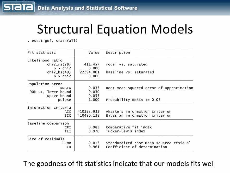
CD 0.961 Coefficient of determination SRMR 0.013 Standardized root mean squared residualSize of residuals TLI 0.970 Tucker-Lewis index CFI 0.983 Comparative fit indexBaseline comparison BIC 410490.138 Bayesian information criterion AIC 410228.932 Akaike's information criterionInformation criteria pclose 1.000 Probability RMSEA <= 0.05 upper bound 0.035 90% CI, lower bound 0.030 RMSEA 0.033 Root mean squared error of approximationPopulation error p > chi2 0.000 chi2_bs(49) 22294.001 baseline vs. saturated p > chi2 0.000 chi2_ms(28) 411.457 model vs. saturatedLikelihood ratio Fit statistic Value Description
. estat gof, stats(all)
The goodness of fit statistics indicate that our models fits well

Structural Equation Models
The residuals are small or zero
ptindex -0.2 0.1 -0.1 0.1 0.0 -0.1 0.0 0.0 0.0 0.0 0.0 credithrs -0.0 -0.0 0.0 0.0 -0.0 -0.0 0.0 0.0 0.0 0.0 male 0.0 -0.0 -0.0 -0.0 0.0 0.0 -0.0 0.0 0.0 instate -0.0 0.0 0.0 -0.0 -0.0 0.0 -0.0 0.0 fygpa -0.0 0.0 -0.0 0.1 -0.0 -0.1 0.0 hsgpa 0.0 -0.0 -0.0 -0.0 0.0 0.0 satq 0.0 0.0 -0.0 -0.0 0.0 satv -0.0 0.0 -0.0 0.0 stipend_c -0.0 -0.0 0.0 scholarshi~c 0.0 0.0 grants_c -0.0 gran scho stip satv satq hsgp fygp inst male cred ptin
Covariance residuals
raw -0.0 -0.0 -0.0 0.0 0.0 0.0 0.0 0.0 0.0 0.0 0.0 gran scho stip satv satq hsgp fygp inst male cred ptin
Mean residuals
Residuals of observed variables
. estat residuals, format(%4.1f)

EPC = expected parameter change cov(e.hsgpa,e.fygpa) 197.553 1 0.00 -.0743199 -.1513768 cov(e.satq,e.fygpa) 32.381 1 0.00 -.0307431 -.0652183 cov(e.satq,e.hsgpa) 364.384 1 0.00 .2558447 .4808539 cov(e.satv,e.fygpa) 332.417 1 0.00 .1032584 .23088 cov(e.satv,e.hsgpa) 33.981 1 0.00 -.089045 -.1763945 cov(e.satv,e.satq) 219.540 1 0.00 -.256884 -.5300054 credithrs 4.963 1 0.03 -.0165768 -.0167176 male 6.309 1 0.01 .0389548 .0188646 instate 10.294 1 0.00 .0550984 .0240733 fygpa 218.432 1 0.00 -.1762143 -.1263594 satq 364.384 1 0.00 .5008192 .5087967 satv 33.981 1 0.00 -.1936382 -.2019313 hsgpa <- fygpa 34.087 1 0.00 -.0711863 -.0502458 hsgpa 364.385 1 0.00 .4616847 .454446 satv 219.539 1 0.00 -.558623 -.5734137 satq <- credithrs 11.401 1 0.00 .0260854 .0252267 male 7.807 1 0.01 -.0449951 -.0208948 instate 5.401 1 0.02 -.0414326 -.0173591 fygpa 363.321 1 0.00 .2438424 .167673 hsgpa 33.981 1 0.00 -.1606859 -.1540867 satq 219.539 1 0.00 -.5028531 -.4898824 satv <- ptindex 5.791 1 0.02 .0010236 .0185995 scholarships_c <- Measurement hsgpa 197.553 1 0.00 -.1341139 -.1870284 satq 32.381 1 0.00 -.0601799 -.0852606 satv 332.417 1 0.00 .2245471 .3265529 fygpa <- Structural MI df P>MI EPC EPC Standard
Modification indices
. estat mindices

Continuous Outcome Models Using sem
• Example Data• Means• Correlation• Linear Regression• Multivariate Regression• Path Analysis and Mediation• Confirmatory Factor Analysis (CFA)• Structural Equation Models (SEM)• Multi-group SEM• SEM For Complex Survey Data

Multigroup SEM
We can also fit models by group and test for invariance of parameters across groups.
sem (Funding -> grants_c@1 scholarships_c stipend_c) ///
(Aptitude -> satv@1 satq hsgpa) ///
(Funding Aptitude -> fygpa) ///
(instate male credithrs ptindex -> fygpa), ///
latent(Funding Aptitude) ///
group(private)
estat ggof
estat ginvariant

Continuous Outcome Models Using sem
• Example Data• Means• Correlation• Linear Regression• Multivariate Regression• Path Analysis and Mediation• Confirmatory Factor Analysis (CFA)• Structural Equation Models (SEM)• Multi-group SEM• SEM For Complex Survey Data
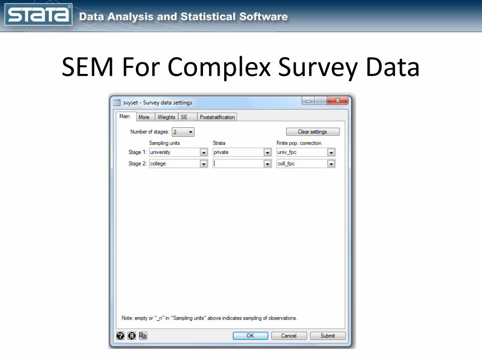
SEM For Complex Survey Data
• We can use sem and gsem to fit models for data that were collected using complex probability samples.
• For example, we might have collected our data by drawing a sample of universities and then colleges within universities.
• We can tell Stata about these features using svy set and our models will be estimated correctly.
SEM For Complex Survey Data

SEM For Complex Survey Data
svyset university [pweight=samplewt], ///
strata(private) ///
fpc(univ_fpc) ///
vce(linearized) ///
singleunit(missing) ///
|| college, ///
fpc(coll_fpc)
svy linearized : sem (Funding -> grants_c@1 scholarships_c stipend_c) ///
(Aptitude -> satv@1 satq hsgpa) ///
(Funding Aptitude -> fygpa) ///
(instate male credithrs ptindex -> fygpa), ///
latent(Funding Aptitude)

Outline
• What is structural equation modeling?
• Structural equation modeling in Stata
• Continuous outcome models using sem
• Multilevel generalized models using gsem
• Demonstrations and Questions
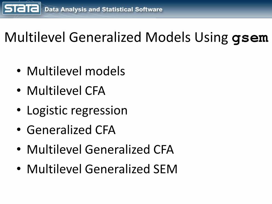
Multilevel Generalized Models Using gsem
• Multilevel models
• Multilevel CFA
• Logistic regression
• Generalized CFA
• Multilevel Generalized CFA
• Multilevel Generalized SEM

Variance Component Model Path Diagram

Variance Component Model SyntaxSyntax using mixed:
Syntax using gsem:
mixed fygpa || university:
gsem (M1[university] -> fygpa), latent(M1)
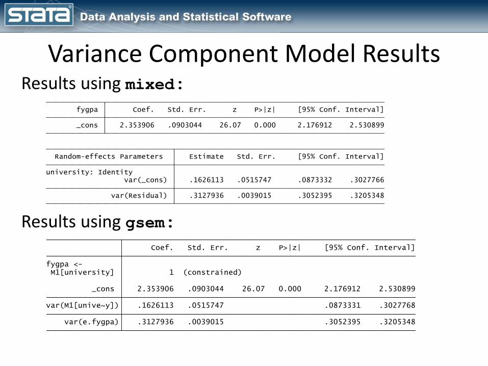
Variance Component Model ResultsResults using mixed:
Results using gsem: var(Residual) .3127936 .0039015 .3052395 .3205348 var(_cons) .1626113 .0515747 .0873332 .3027766university: Identity Random-effects Parameters Estimate Std. Err. [95% Conf. Interval]
_cons 2.353906 .0903044 26.07 0.000 2.176912 2.530899 fygpa Coef. Std. Err. z P>|z| [95% Conf. Interval]
var(e.fygpa) .3127936 .0039015 .3052395 .3205348 var(M1[unive~y]) .1626113 .0515747 .0873331 .3027768 _cons 2.353906 .0903044 26.07 0.000 2.176912 2.530899 M1[university] 1 (constrained)fygpa <- Coef. Std. Err. z P>|z| [95% Conf. Interval]

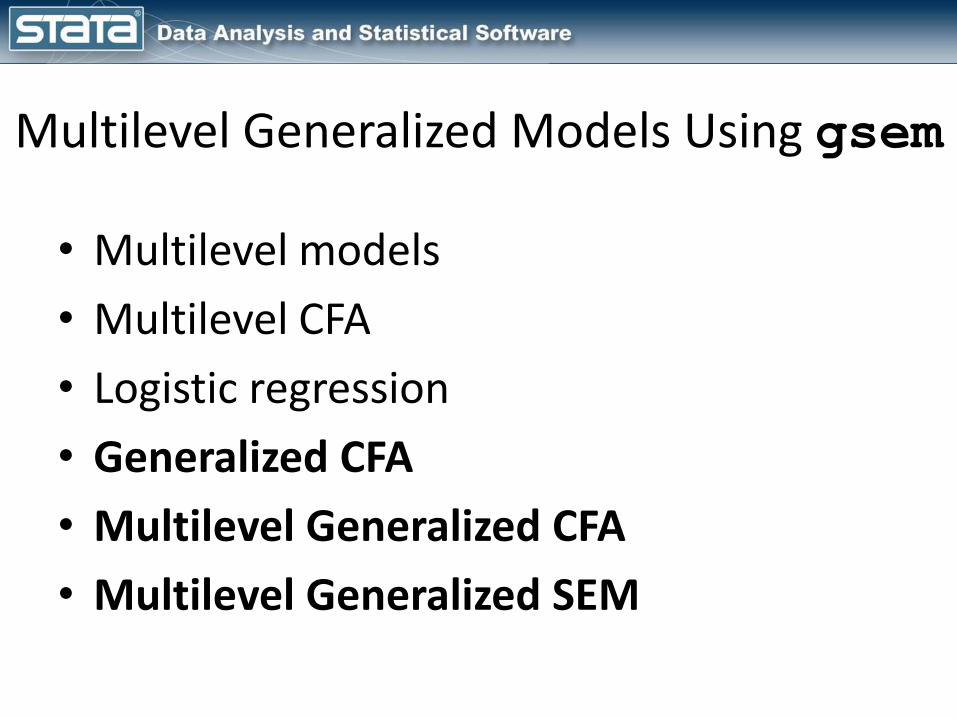
Multilevel Generalized Models Using gsem
• Multilevel models
• Multilevel CFA
• Logistic regression
• Generalized CFA
• Multilevel Generalized CFA
• Multilevel Generalized SEM

Multilevel CFA Path Diagram

Multilevel CFA Results
var(e.stipend_c) .6626266 .0096384 .6440023 .6817894var(e.scholar~c) .2964019 .0089246 .2794162 .3144201 var(e.grants_c) .4950738 .0092272 .4773152 .5134932 var(student) .4963372 .0125068 .4724198 .5214656var(M1[unive~y]) 7.99e-11 . . . _cons -.0086983 .00877 -0.99 0.321 -.0258873 .0084907 student .821042 .0146714 55.96 0.000 .7922866 .8497974 M1[university] 1 (constrained)stipend_c <- _cons -.0064351 .0087012 -0.74 0.460 -.0234891 .010619 student 1.175532 .0180882 64.99 0.000 1.14008 1.210985 M1[university] 1 (constrained)scholarshi~c <- _cons -.0041953 .0087432 -0.48 0.631 -.0213317 .0129411 student 1 (constrained) M1[university] 1 (constrained)grants_c <- Coef. Std. Err. z P>|z| [95% Conf. Interval]
gsem (student -> grants_c@1 scholarships_c stipend_c) ///
(M1[university]@1 -> grants_c scholarships_c stipend_c), ///
covstruct(_lexogenous, diagonal) from(b) latent(student M1) ///
means(student@0 M1[university]@0) nocapslatent

Multilevel Generalized Models Using gsem
• Multilevel models
• Multilevel CFA
• Logistic regression
• Generalized CFA
• Multilevel Generalized CFA
• Multilevel Generalized SEM

Logistic Regression Path Diagram

Logistic Regression Syntax
Syntax using logit or logistic:
Syntax using gsem:
logit ret_yr1 instate male credithrs ptindex
logistic ret_yr1 instate male credithrs ptindex
gsem ret_yr1 <- instate male credithrs ptindex, ///
family(bernoulli) link(logit)
gsem ret_yr1 <- instate male credithrs ptindex, logit
estat eform

Logistic Regression Results
Results using logistic:
Results using gsem and estat eform:
_cons .0394908 .0184686 -6.91 0.000 .0157912 .0987588 ptindex .9984765 .0016018 -0.95 0.342 .9953419 1.001621 credithrs 1.376276 .0400066 10.99 0.000 1.300056 1.456964 male 1.093629 .0643822 1.52 0.128 .9744497 1.227384 instate 1.898841 .1134222 10.74 0.000 1.689057 2.134681 ret_yr1 exp(b) Std. Err. z P>|z| [95% Conf. Interval]
_cons .0394908 .0184686 -6.91 0.000 .0157912 .0987588 ptindex .9984765 .0016018 -0.95 0.342 .9953419 1.001621 credithrs 1.376276 .0400066 10.99 0.000 1.300056 1.456964 male 1.093629 .0643822 1.52 0.128 .9744497 1.227384 instate 1.898841 .1134222 10.74 0.000 1.689057 2.134681 ret_yr1 Odds Ratio Std. Err. z P>|z| [95% Conf. Interval]
Multilevel Generalized Models Using gsem
• Multilevel models
• Multilevel CFA
• Logistic regression
• Generalized CFA
• Multilevel Generalized CFA
• Multilevel Generalized SEM
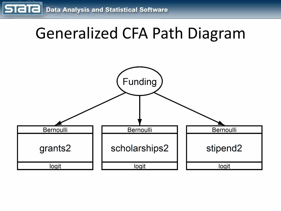
Generalized CFA Path Diagram
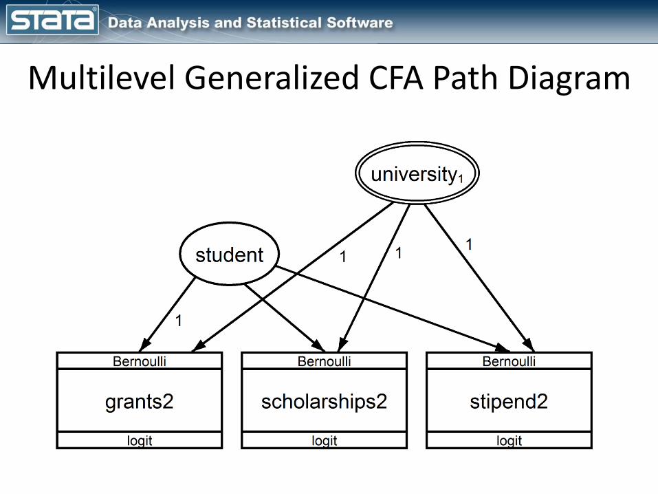
Multilevel Generalized CFA Path Diagram
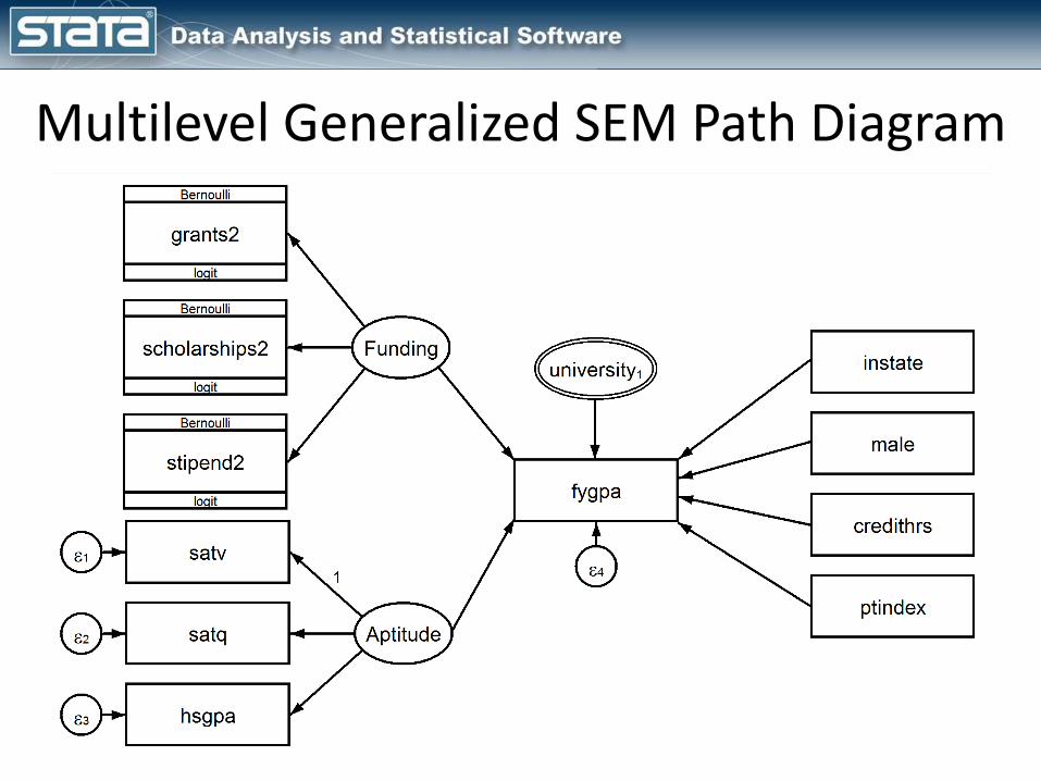
Multilevel Generalized SEM Path Diagram

Multilevel Generalized Models Using gsem
• Multilevel models
• Multilevel CFA
• Logistic regression
• Generalized CFA
• Multilevel Generalized CFA
• Multilevel Generalized SEM

Outline
• What is structural equation modeling?
• Structural equation modeling in Stata
• Continuous outcome models using sem
• Multilevel generalized models using gsem
• Demonstrations and Questions

References and Further Reading1. Stata 14 Structural Equation Modeling Reference Manual:
www.stata.com/manuals14/sem.pdf
2. Acock, A.C. (2013) Discovering Structural Equation Modeling Using Stata, Revised Edition . College Station, TX: Stata Press.
3. Bollen, K.A. (1989) Structural Equations With Latent Variables. New York: Wiley
4. Hu, L., and Bentler, P. M. (1999). Cutoff criteria for fit indexes in covariance structure analysis: Conventional criteria versus new alternatives. Structural Equation Modeling, 6, 1–55.
5. Kline, R.B. (2015). Principles and Practice of Structural Equation Modeling , 4th Ed. New York: Guilford Press
6. Matsueda, R.L. (2012). Key Advances in the History of Structural Equation Modeling. Handbook of Structural Equation Modeling. 2012. Edited by R. Hoyle. New York, NY: Guilford Press
7. Rabe-Hesketh, S., and A. Skrondal. (2012) Multilevel and Longitudinal Modeling Using Stata. 3rd ed. College Station, TX: Stata Press.
Thank you!
Questions?
You can download the slides, dataset, and do-file here:https://tinyurl.com/2019SEM
My email address is:[email protected]