introduction to supersymmetry phys-f-417 - personal...
TRANSCRIPT

Introduction to SupersymmetryPHYS-F-417
Riccardo ArgurioUniversite Libre de Bruxelles
October 20, 2017

2

Contents
1 Introduction 71.1 Motivating supersymmetry . . . . . . . . . . . . . . . . . . . . 71.2 Plan of the lecture notes . . . . . . . . . . . . . . . . . . . . . 141.3 Further reading . . . . . . . . . . . . . . . . . . . . . . . . . . 14
2 The superalgebra 172.1 A graded extension of the Poincare algebra . . . . . . . . . . . 172.2 Representations of the Lorentz group . . . . . . . . . . . . . . 182.3 A first look at the superalgebra . . . . . . . . . . . . . . . . . 25
2.3.1 Basic consequences of the superalgebra . . . . . . . . . 272.4 Representations of the superalgebra . . . . . . . . . . . . . . . 29
2.4.1 Massless supermultiplets . . . . . . . . . . . . . . . . . 292.4.2 Supermultiplets of extended supersymmetry . . . . . . 312.4.3 Massive supermultiplets . . . . . . . . . . . . . . . . . 33
3 Supersymmetric field theories 373.1 The theory for the scalar multiplet . . . . . . . . . . . . . . . 37
3.1.1 Supersymmetry variations on scalar and fermionic fields 383.1.2 Introducing auxiliary fields . . . . . . . . . . . . . . . . 433.1.3 Supersymmetric mass terms . . . . . . . . . . . . . . . 453.1.4 Supersymmetric interactions . . . . . . . . . . . . . . . 47
3.2 The theory for the vector multiplet . . . . . . . . . . . . . . . 48
4 Superspace and superfields 534.1 Introducing superspace and superfields . . . . . . . . . . . . . 53
4.1.1 Supersymmetry transformations as translations in su-perspace . . . . . . . . . . . . . . . . . . . . . . . . . . 56
4.1.2 Manifestly supersymmetry invariant action . . . . . . . 59
3

4 CONTENTS
4.2 Chiral superfields . . . . . . . . . . . . . . . . . . . . . . . . . 614.2.1 Action for a chiral superfield . . . . . . . . . . . . . . . 644.2.2 Superpotential . . . . . . . . . . . . . . . . . . . . . . 674.2.3 Equations of motion for chiral superfields . . . . . . . . 69
4.3 Real superfields . . . . . . . . . . . . . . . . . . . . . . . . . . 714.3.1 Gauge symmetry and the vector multiplet . . . . . . . 724.3.2 The action and the gaugino chiral superfield . . . . . . 784.3.3 Equations of motion for real superfields . . . . . . . . . 834.3.4 Fayet-Iliopoulos term . . . . . . . . . . . . . . . . . . . 85
5 Supersymmetric gauge theories 875.1 Most general SUSY gauge theory with matter . . . . . . . . . 87
5.1.1 An abelian example: SQED . . . . . . . . . . . . . . . 905.1.2 Non-abelian gauge group . . . . . . . . . . . . . . . . . 945.1.3 Most general action in components . . . . . . . . . . . 96
5.2 Scalar potential and moduli space of vacua . . . . . . . . . . . 975.2.1 General characterization of the moduli space . . . . . . 101
5.3 The example of SQCD . . . . . . . . . . . . . . . . . . . . . . 1045.3.1 R-symmetry . . . . . . . . . . . . . . . . . . . . . . . . 1055.3.2 The classical vacua of SQCD . . . . . . . . . . . . . . . 107
5.4 A brief look at the MSSM . . . . . . . . . . . . . . . . . . . . 109
6 Radiative corrections and non-renormalization theorems 1136.1 Superfield propagators . . . . . . . . . . . . . . . . . . . . . . 113
6.1.1 Formulation with component fields . . . . . . . . . . . 1146.1.2 Formulation with superfields . . . . . . . . . . . . . . . 119
6.2 Some radiative corrections . . . . . . . . . . . . . . . . . . . . 1226.3 General results on renormalization . . . . . . . . . . . . . . . 125
6.3.1 Super-Feyman rules . . . . . . . . . . . . . . . . . . . . 1276.3.2 Non-renormalization theorem . . . . . . . . . . . . . . 128
6.4 Renormalization of the real superfield . . . . . . . . . . . . . . 1316.5 Holomorphy and non-renormalization . . . . . . . . . . . . . . 133
7 Supersymmetry breaking 1377.1 Spontaneous SUSY breaking . . . . . . . . . . . . . . . . . . . 138
7.1.1 Vacuum energy and f - and d-terms . . . . . . . . . . . 1387.1.2 The SUSY breaking vacuum and the goldstino . . . . . 1407.1.3 The supertrace theorem . . . . . . . . . . . . . . . . . 142
CONTENTS 5
7.2 Examples of SUSY breaking theories . . . . . . . . . . . . . . 1447.2.1 d-term breaking: Fayet-Iliopoulos model . . . . . . . . 1457.2.2 f -term breaking: O’Raifeartaigh model . . . . . . . . . 146
7.3 Quantum corrections to the vacuum energy . . . . . . . . . . . 1497.3.1 The case of the O’Raifeartaigh model . . . . . . . . . . 151
7.4 SUSY breaking and R-symmetry . . . . . . . . . . . . . . . . 1537.5 Explicit SUSY breaking: soft terms . . . . . . . . . . . . . . . 155
7.5.1 The mediation paradigm . . . . . . . . . . . . . . . . . 1577.6 Dynamical SUSY breaking . . . . . . . . . . . . . . . . . . . . 158

6 CONTENTS

Chapter 1
Introduction
Disclaimer (2009): These notes are being written in the beginning of 2009.LHC should start running hopefully within a year. Then, it is likely that somedata concerning supersymmetry will soon start to be available. The mostfavourable outcome is a Nobel prize awarded already in 2011. Then therewould be little need to motivate further the subject of these lectures. On theother hand the outcome could be the opposite, ruling out supersymmetryin the (accessible) real world. Then these lectures are concerned with abeautiful mathematical construction which allows us to better understandthe quantum properties of field theories. Of course, it is most likely that thereal outcome of LHC will be just half way between the two options above..
Disclaimer (2015): Well, it turned out to be, of course, in the middle. SUSYis not ruled out, but its most straightforward versions are having a hard time,in particular to justify their usefulness.. Stay tuned!
1.1 Motivating supersymmetry
Supersymmetry is an organizing principle for quantum field theories whichaddresses both theoretical and technical aspects of them.
In all generality, symmetries (both internal and space-time) implementconstraints on the structure of the theory, and on its quantum corrections.In particular, they help in answering the following questions:
• Why is the spectrum as it is?
• Why are there some couplings, while others are vanishing?
7
8 CHAPTER 1. INTRODUCTION
• Why some quantities are much smaller than others (i.e. there are hi-erarchies)?
Supersymmetry is a very powerful symmetry, which extends the usualPoincare space-time symmetry. In this sense it is more powerful than aglobal internal symmetry. Particles are commonly divided into bosons (ofinteger spin, such as scalars and vectors) and fermions (of half-integer spin,which herein will always be spin 1/2). Supersymmetry (also called SUSY)relates these two kinds of particles. It must then mix non-trivially withthe Poincare space-time symmetry since it relates particles which belong todifferent representations of the Lorentz group, since the latter are denotedby their spin.
As we will see, SUSY implements strong constraints on the spectrum andon the couplings of a field theory. Thus, it goes towards the goal of formu-lating a unique theory of all interactions, where everything is constrainedand nothing is left to (arbitrary) choice. Actually, it goes very close to thisaim when gravity is taken into account and the theory becomes the one ofsupergravity. Moreover, if one wants a setting in which gravity is consis-tently quantized, one has to resort to string theory. It is amusing to notethat in turn, string theories are fully consistent only when supersymmetryis present–one then talks of superstring theory. Actually, it is really in thiscontext that SUSY appeared first in physics, during the early 70s.
At a more technical level, SUSY helps also in addressing the questionof quantum corrections and hierarchies, which is related to the notion ofnaturalness, as opposite to fine tuning: One wants the parameters in thetheory describing Nature to be close to generic values. This is intimatelyrelated to the symmetry in the spectrum relating bosons and fermions.
Take e.g. the vacuum energy in the most simple quantum mechanicalmodel. For a bosonic oscillator, we have
HB =1
2(a†a+ aa†).
At the quantum level, i.e. when [a, a†] = ~, we have that the vacuum state,defined by a|0〉 = 0, is such that
HB|0〉 =1
2aa†|0〉 =
1
2(a†a+ ~)|0〉 =
1
2~|0〉
so that the vacuum energy is
Evac,B =1
2~.

1.1. MOTIVATING SUPERSYMMETRY 9
In field theory, we basically have oscillators at every space-time point or,in other words (and after a Fourier transform), of every frequency. Summingover all of them will give a very large vacuum energy density, roughly pro-portional to the 4th power of the cut off scale beyond which the theory is nolonger well defined, usually taken to be the Plack scale Mp.
1
Now consider a fermionic oscillator, with Hamiltonian and anti-commu-tation relations as follow
HF =1
2(α†α− αα†), α, α† = ~.
If the vacuum is defined by α|0〉 = 0, we get
HF |0〉 = −1
2αα†|0〉 = −1
2(~− α†α)|0〉 = −1
2~|0〉
so that the vacuum energy is now
Evac,F = −1
2~.
It is negative.2
So, if for every frequency we have
Htot = HB +HF = a†a+ α†α
thenEtot = 0
and the total energy density vanishes.This is one instance of the simplifications due to SUSY, and also an
example of how a symmetry (implicit but present in the above) can constraina quantity such as the vacuum energy. The lesson is that quantum correctionsare sometimes vanishing, or at least more constrained. As we will see, thisis also true for radiative corrections, for instance to the mass of particles.
One vexing problem of the Standard Model (SM) is the hierarchy betweenthe scale of Electro-weak interactions MEW ∼ 100 GeV and the Planck scale
1Indeed, trading energy scales for length scales, it makes no sense to consider anyquantum field theory at distances shorter than the Planck length (Lp = M−1p in therelevant units), where quantum gravity effects affect the notion of space-time itself.
2Note that HFα†|0〉 = (α†α − 1
2~)α†|0〉 = (α†~ − 12~α
†)|0〉 = 12~α
†|0〉 so that indeed|0〉 is the ground state.
10 CHAPTER 1. INTRODUCTION
Mp ∼ 1019 GeV. Roughly speaking, and without entering into the details,the Electro-weak scale depends in particular on a parameter of the SM, theHiggs scalar mass, which has to be fine tuned by many orders of magnitude(with respect to Mp, of course) in order to give the experimentally observedscale. Even more troubling, quantum corrections tend to restore this massto its “natural” scale Mp, due to quadratic divergencies. Namely, there arefor instance one-loop corrections to the Higgs scalar two-point function, withquarks and leptons running in the loop. If H is the Higgs scalar, ψ, ψ aresuch representative fermions, and there is an interaction term LSM ⊃ λHψψ,then the leading UV divergence in the two point function of H is proportionalto
λ2
∫ ΛUV
d4p1
p
1
p− k∼ λ2Λ2
UV ,
where p is the momentum running in the loop, k the incoming momentumand ΛUV the UV cut-off of the theory.
Supersymmetry comes to the rescue by adding, for every fermion, a newscalar particle, call it Sψ, along with a new vertex involving H, LSUSYSM ⊃µH2S2
ψ. There is then a new one-loop correction to the two point functionfor H, with Sψ running in the loop. It also has a quadratic divergence,proportional to:
µ
∫ ΛUV
d4p1
p2∼ µΛ2
UV .
It is easy to conceive that by tuning the couplings µ ∝ λ2, the two leadingcorrections can cancel. This is exactly what supersymmetry does!
So, SUSY can help in maintaining a hierarchy, protecting it from quantumcorrections.
Explaining the hierarchy is on the other hand more involved. Let us justmention a natural way to generate large hierarchies in quantum field theory.Consider for instance a scale generated dynamically by dimensional transmu-tation along a renormalization group flow. This is the case for non-abeliangauge theories, where the one-loop beta function for the gauge coupling greads
β(g) ≡ µdg
dµ= − b0
16π2g3 +O(g5).
We have that for asymptotically free theories, such as QCD, b0 > 0 and the

1.1. MOTIVATING SUPERSYMMETRY 11
above differential equation can be integrated so that
8π2
g2(µ)=
8π2
g2(ΛUV )+ b0 log
µ
ΛUV
.
A dynamical scale is obtained by running downwards the above expressionuntil the coupling becomes infinite. Reversing then the equation, we obtainthat the scale defined in such a way is given by
Λdyn = ΛUV e− 8π2
b0g2(ΛUV ) .
The coefficient b0 is of the order of the rank of the gauge group, while g(ΛUV )can be naturally taken to be < 1 and reasonably small. Then the exponentialfactor in the expression above can be very small, even 10−15 to mention oneinteresting ratio.
The upshot is that some hierarchies, like the one between Λdyn and ΛUV ,can be naturally explained. For instance, the dynamical scale of QCDΛQCD ∼ 250 MeV gives the order of magnitude of the masses of hadronsand baryons, and the hierarchy between ΛQCD and Mp is explained by theasymptotic freedom of QCD. Thus, for SUSY to explain the hierarchy prob-lem in the Electro-weak sector, the mass of the Higgs scalar must be relatedto a dynamically generated scale. We will see shortly how SUSY can beassociated to such a scale.
Another, independent, motivation for supersymmetry is found in the phe-nomenological arena, and has to do with the idea of Grand Unification (a.k.a.GUT, for Grand Unified Theory). The idea is that the gauge group of theStandard Model is embedded in a simple gauge group:
GSM = SU(3)× SU(2)× U(1) ⊂ GGUT
One easily realizes that the two smallest simple groups are:
GGUT = SU(5), SO(10), . . .
Of course any larger group containing the above is also suitable, but theabove groups are the ones yielding a minimal extension of SM physics. (Inparticular, matter representations of GGUT split up into just the matter rep-resentations of GSM .)
A necessary condition for unification to take place, is that the breaking ofthe gauge symmetry from GGUT to GSM is consistent. From first principles,

12 CHAPTER 1. INTRODUCTION
it has to happen in the following way. In the UV, there is only one gaugegroup, and hence a single coupling, which runs as prescribed by its betafunction (one assumes that the GUT is asymptotically free). Going towardsthe IR, at some scale MGUT the gauge group GGUT is broken to GSM bythe Brout-Englert-Higgs mechanism (just as SU(2) × U(1)Y is broken toU(1)EM at MEW ). At this stage, the couplings of the 3 groups in GSM startrunning independently, according to each one’s beta function. However, it isimportant to note that they share the same boundary conditions at MGUT .This is referred to as gauge coupling unification. Hence, in order for the GUTidea to work, one has to take the observed values of the gauge couplings inGSM at, say, the Electro-weak scale MEW , and run them upwards using theirbeta functions. Doing this will draw three lines3 in the plot of 1/g2
i againstlog µ. GUT is then an acceptable idea if the three lines meet.
Now, if one uses the beta functions of the SM (which implies conjecturingthat there is no new physics from the MEW scale onwards to a putativeMGUT scale, since new heavy charged particles would contribute to the betafunctions at scales roughly higher than their mass), the three lines comeclose but actually miss. Now three lines in a plane do not have to meet ata common point, and do not even have to come close to that. Hence thisclose miss does not rule out completely GUTs, at least at the level of wishfulthinking. But SUSY rescues the idea altogether. Indeed, using the spectrumof the minimal SUSY extension of the SM, called the MSSM (to be definedlater..), which means that a precise set of new particles starts contributing tothe beta functions at scales slightly higher than MEW (recall that SUSY hasto kick in around MEW in order to address the hierarchy problem), then thethree lines do meet! Of course, there are error bars, but the meeting seemsindeed reasonable and it predicts a GUT scale of MGUT ∼ 1016 GeV.
Let us also briefly mention that one last interesting outcome of SUSYis the prediction of the existence of a stable, neutral particle (the lightestsupersymmetric particle, or LSP) which is usually a viable candidate fordark matter.
There are also theoretical motivations for studying supersymmetry. Inparticular, the study of SUSY gauge theories in general (and not only theMSSM) has had many successes. SUSY is such a strong constraint on thestructure (both at the classical and quantum levels) of the theory, that ishas been possible to obtain results in the strong coupling regime (i.e. at low-
3At least at one-loop.

1.1. MOTIVATING SUPERSYMMETRY 13
energies for asymptotically free theories, when E ∼ Λdyn and g → ∞) thatcannot be obtained, for instance, in non-supersymmetric QCD. This moti-vation, though more remote from observational constraints, is on the otherhand somewhat more stable, in that the beautiful mathematical structure ofSUSY and its implications for quantum gauge theories are independent onthe likelihood of the LHC to work properly..
Until now, we refrained to address one important aspect, that shouldhowever be obvious: supersymmetry is not yet observed. Again, LHC aside,the important point here is that the SM, which reproduces so well all theobservations done until now (say, below few TeVs), is not supersymmetric.In particular, SUSY must relate bosons and fermions, but as we will see itcommutes with any gauge group (and, for that matters, also with genericglobal symmetry groups), so that superpartners must belong to the samerepresentations. It is obvious that bosons and fermions in the SM do notbelong to even slightly similar representations. Then, the most pressingquestion to be addressed is ‘how is SUSY broken?’
There are essentially two options:
i) SUSY is broken explicitely, i.e. by non-SUSY terms in the Lagrangian,but in a way that its virtues are not (completely) spoiled. Such breakingis called soft SUSY breaking.
ii) SUSY is broken spontaneously (or, equivalently, dynamically, where thetwo terminologies subtly refer to the breaking being due, respectively,to a classical or a quantum mechanism): the theory is SUSY but the(classical or quantum) vacuum is not. This is somewhat nicer becausein formulating the theory we can use all the constraints imposed bySUSY. Many of its consequences are also still valid. Such breaking iscalled spontaneous (or dynamical) SUSY breaking.
In both cases, it is important to note that there will be a scale associated tothe SUSY breaking effects, which we will call MSUSY . It can be for instancethe scale of a mass (soft), or of a VEV (spontaneous). For E > MSUSY thetheory is SUSY, while for E < MSUSY it is not. In a way, MSUSY will workas an effective cut-off for the corrections which are protected by SUSY.
In particular, it will be phenomenologically important to obtainMSUSY MGUT ,Mp so as to protect (and possibly implement) the hierarchy. Natural-ness thus seems to point towards dynamical SUSY breaking, where MSUSY
is linked to Λdyn of some gauge group, possibly hidden.

14 CHAPTER 1. INTRODUCTION
To conclude, the motivation to study supersymmetry should be matchedby an equal motivation to study how supersymmetry can be broken.
1.2 Plan of the lecture notes
These lecture notes are organized as follows.In Chapter 2 we review the superalgebra as an extension of the Poincare
algebra, and its representations, i.e. the supermultiplets containing bosonsand fermions.
In Chapter 3 we implement supersymmetry at the level of Lagrangianfield theories, and provide simple examples of such theories with and withoutgauge fields.
In Chapter 4 we turn to formulating manifestly SUSY invariant actionsfor the same field theories, thus introducing superspace and superfields.
In Chapter 5 we discuss the most general SUSY gauge theory with matter,reviewing its classical properties such as the moduli space of SUSY vacua,and providing the examples of Super-QCD (SQCD) and the MSSM.
In Chapter 6 we review the perturbative quantization of SUSY field the-ories, discussing radiative corrections and non-renormalization theorems.
In Chapter 7 we discuss various mechanisms of supersymmetry breaking.
1.3 Further reading
It can be useful to list some references, essentially reviews or books, thatcan help in comprehending the subject of these notes. Most of the referencesbelow were indeed used to form the material presented here. Additionalreferences on specific issues may be given at a later stage.
• A. Bilal, “Introduction to supersymmetry,” arXiv:hep-th/0101055.
• P. C. West, “Introduction to supersymmetry and supergravity,” Singa-pore, Singapore: World Scientific (1990) 425 p.
• J. Wess and J. Bagger, “Supersymmetry and supergravity,” Princeton,USA: Univ. Pr. (1992) 259 p.
• S. Weinberg, “The quantum theory of fields. Vol. 3: Supersymmetry,”Cambridge, UK: Univ. Pr. (2000) 419 p.
1.3. FURTHER READING 15
• P. Argyres, “Lectures on Supersymmetry,” available athttp://www.physics.uc.edu/~argyres/661/index.html.
• J. Terning, “Modern supersymmetry: Dynamics and duality,” Oxford,UK: Clarendon (2006) 324 p.
• S. P. Martin, “A Supersymmetry Primer,” arXiv:hep-ph/9709356.
• R. Argurio, G. Ferretti and R. Heise, “An introduction to supersym-metric gauge theories and matrix models,” Int. J. Mod. Phys. A 19(2004) 2015 [arXiv:hep-th/0311066].
• K. A. Intriligator and N. Seiberg, “Lectures on Supersymmetry Break-ing,” Class. Quant. Grav. 24 (2007) S741 [arXiv:hep-ph/0702069].
The references are essentially ordered by closeness in spirit to these notes.

16 CHAPTER 1. INTRODUCTION

Chapter 2
The superalgebra
In this chapter we introduce the algebraic structure on which supersymmetryis based, that is the superalgebra. Since it is an extension of the space-timePoincare symmetry, we first review some basic notions on the representa-tions of the Lorentz group. We then present the superalgebra, and derivethe first simple physical consequences for the spectrum of a supersymmetrictheory. We then construct representations of the superalgebra, also calledsupermultiplets, both massless and massive. In this chapter, we will alsobriefly mention extended superalgebras, which however will not be dealt within the rest of the notes.
2.1 A graded extension of the Poincare alge-
bra
In general, under mild assumptions, the Poincare algebra cannot mix non-trivially with other symmetries. In other words, it cannot be embedded ina larger symmetry algebra. This is the main conclusion of the Coleman-Mandula theorem of the ’60s. In a nutshell, it says that if there are extraspace-time symmetries (i.e. extra symmetries mixing non-trivially with thePoincare generators, which means that they are in non-trivial representationsof the Lorentz group), then they would constrain so much the S-matrix thatit would necessarily be trivial. It has to be noted that this theorem holds
17

18 CHAPTER 2. THE SUPERALGEBRA
in four dimensions.1 Of course, a trivial S-matrix means that the theory isfree, and no interactions make the theory a rather dull one. Hence, the onlyextensions which are allowed are the ones by global internal symmetries, i.e.whose generators are spin 0 scalars.
Now, the Coleman-Mandula theorem is true for bosonic symmetries. Ithas one exception if one considers graded extensions of the Poincare algebra,that is algebras involving even and odd operators such that
[E,E] = E, [E,O] = O, O,O = E,
with E any even operator, O any odd operator and , the anticommutator.It then turns out that allowing for odd operators, the Coleman-Mandulatheorem is still at work and implies that the only such extra generators onecan add have spin 1/2. This is a theorem by Haag, Lopuszanski and Sohnius.
Very schematically, one can introduce a spin-1/2 generator Q which sat-isfies the following (anti)commutation relations with the momentum P :
[P,Q] = 0, Q,Q = P.
The operator Q being of spin-1/2, it relates states belonging to represen-tations of spin s to ones of spin s ± 1
2. By the relation between spin and
statistics, it then relates bosons to fermions and vice-versa.Since fermions, and spinors, are crucial to SUSY, we need to review some
facts and notation about representations of the Poincare group, in order toproceed and be more precise.
2.2 Representations of the Lorentz group
Let us anticipate that we will use consistently 2-component Weyl spinorsthroughout these notes. Indeed, the usual Dirac spinor is actually a reduciblerepresentation of the Lorentz group. This said, we can start reviewing thePoincare algebra.
The commutation relations are (µ = 0, 1, 2, 3):
[Pµ, Pν ] = 0 (2.1)
[Mµν ,Mρσ] = −iηµρMνσ − iηνσMµρ + iηµσMνρ + iηνρMµσ (2.2)
[Mµν , Pρ] = −iηµρPν + iηνρPµ (2.3)
1It has an important exception concerning theories where all degrees of freedom aremassless (the space-time symmetry becomes then the conformal group).

2.2. REPRESENTATIONS OF THE LORENTZ GROUP 19
Here the generators satisfy:
Mµν = −Mνµ, M †ij = Mij, M †
0i = −M0i, P †µ = Pµ, (2.4)
i.e. they are hermitian except for the boost generators (this is due to thenon-compactness of the Lorentz group). Moreover, we take the metric to be
ηµν = diag(+,−,−,−). (2.5)
Let us now consider more closely the algebra of the Mµν , that is theSO(1, 3) Lorentz algebra. Consider the split to the spatial indices i = 1, 2, 3(and notice that ηij = −δij). The Mij are 3 generators satisfying
[Mij,Mkl] = iδikMjl + iδjlMik − iδilMjk − iδjkMil (2.6)
If we writeMij = εijkJk (2.7)
that is, M12 = J3,M23 = J1,M31 = J2, we obtain
[Ji, Jj] = iεijkJk (2.8)
the algebra of SU(2).Now we can also rename the other generators as M0i = Ki and find for
their commutation relations
[Mij,M0k] = iδjkMi0 − iδikMj0
which givesεijl[Jl, Kk] = −iδjkKi + iδikKj
and finally[Ji, Kj] = iεijkKk.
We also have[M0i,M0j] = −iMij
which gives[Ki, Kj] = −iεijkJk.
To summarize, we have rewritten the commutation relations of SO(1, 3) as:
[Ji, Jj] = iεijkJk, [Ji, Kj] = iεijkKk, [Ki, Kj] = −iεijkJk. (2.9)

20 CHAPTER 2. THE SUPERALGEBRA
We can now form the following complex generators
J±i =1
2(Ji ± iKi), (2.10)
which are hermitian, and satisfy (J±i )∗ = −J∓i (we must take all the Ji andKi to be imaginary, in order for all rotation and boost parameters to be real).Let us compute their own commutation relations:
[J±i , J±j ] =
1
4iεijkJk − (−iεijkJk)± i(iεijkKk)± i(−iεjikKk)
= iεijk1
2(Ji ± iKi)
= iεijkJ±k
while
[J±i , J∓j ] =
1
4iεijkJk + (−iεijkJk)∓ i(iεijkKk)± i(−iεjikKk)
= 0
We have thus established that the Lorentz group can be rewritten as
SO(1, 3) = SU(2)× SU(2)∗.
This is of course a very well-known fact in the theory of Lie algebras, where atthe level of complex algebras one writes that SO(4) = SU(2)×SU(2). Herewe are concerned with a specific real form of SO(4,C). It is also sometimesuseful to note (or familiar) that
SU(2)× SU(2)∗ = SL(2,C)
the group of the 2× 2 complex matrices of unit determinant.Here, it will suffice to recall that representations of the Lorentz group
can be classified by two SU(2) spins (s, s′) of SU(2) × SU(2)∗. Then, thecomplex conjugation of the second SU(2) is understood with the followingmeaning, when considering an arbitrary representation:
(s, s′)∗ = (s′, s).
The smallest representations are the spinorial ones:
(12, 0) and (0, 1
2).

2.2. REPRESENTATIONS OF THE LORENTZ GROUP 21
We will denote them as 2-vectors with indices, respectively
α = 1, 2 and α = 1, 2.
We will thus write our Weyl spinors as ψα and ψα, with the understandingthat
(ψα)∗ = ψα.
Higher dimensional representations appear taking (tensor) products ofthis two basic (fundamental) representations. For instance:
(12, 0)⊗ (0, 1
2) = (1
2, 1
2),
which is an irreducible 4-dimensional representation of SO(1, 3), so it cannotbe anything else than a vector vµ.
Indeed, we can write the product of two spinors as
ψαψα ≡ vαα
a 2×2 matrix, thus with 4 components. The latter can in turn be decomposedinto a basis of 2×2 matrices. As such a basis, we can choose the Pauli matricessupplemented by the identity:
σµαα = (I,−τi), (2.11)
which means explicitly
σ0 =
[1 00 1
], σ1 =
[0 −1−1 0
], σ2 =
[0 i−i 0
], σ3 =
[−1 00 1
].
(2.12)We now see that the product of two spinors is indeed a vector:
ψαψα ≡ vαα = σµααvµ.
Another example is the following product:
(12, 0)⊗ (1
2, 0) = (0, 0)⊕ (1, 0).
The right hand side thus corresponds to a singlet together with a 3-dimensio-nal representation of SO(1, 3). As a product of two spinors, we can write:
ψαχβ = εαβs+ tαβ, with tαβ = tβα.

22 CHAPTER 2. THE SUPERALGEBRA
εαβ = −εβα is the invariant tensor of SU(2) (one can check that, using thefact that the SU(2) matrices have determinant 1).
Then, what is tαβ? It should be an integer spin representation of SO(1, 3),so it should be associated with a bosonic field with some Lorentz symmetry.Consider for instance an antisymmetric tensor Tµν = −Tνµ. It has 6 indepen-dent components. However, in SO(1, 3) we also have an invariant completelyantisymmetric tensor, written as εµνρσ and sometimes called the Levi-Civitatensor. We adopt the convention that
ε0123 = ε0123 = 1.
It can be used to define a dual tensor
Tµν =i
2εµνρσT
ρσ.
Note that
˜Tµν =i
2εµνρσT
ρσ =i
2εµνρσ
(− i
2ερσλτTλτ
)= Tµν .
The dual tensor is also antisymmetric Tµν = −Tνµ and hence also has 6components. We can define:
Tµν =1
2
(Tµν +
i
2εµνρσT
ρσ
)+
1
2
(Tµν −
i
2εµνρσT
ρσ
)=
1
2T+µν +
1
2T−µν .
We have thus
T±µν =i
2εµνρσT
±ρσ = ±T±µν
which means that these two tensors are (anti)self-dual. Each one has only 3independent (generally complex) components.
The representation (1, 0) corresponds to a self-dual tensor like T+µν , while
(0, 1) = (1, 0)∗ corresponds to an anti-self-dual tensor like T−µν or (T+µν)∗.
Indeed, one has(1
2, 1
2)⊗A (1
2, 1
2) = (1, 0)⊕ (0, 1).
Going back now to εαβ, we note that it can be used to raise and lowerindices. In the process we will fix a good deal of notation and conventions.

2.2. REPRESENTATIONS OF THE LORENTZ GROUP 23
First of all, we define the SU(2) antisymmetric tensor to have the followingvalues:
ε12 = ε12 = ε21 = ε21 = 1.
Then, we define:
ψα = εαβψβ, ψα = εαβψβ, ψα = εαβψβ, ψα = εαβψ
β.
In other words, adjacent indices are always contracted with the epsilon ten-sor on the left. [Exercise: count the number of arbitrary signs that oneis fixing with these conventions..] Note that the fact that, for instance,ψα = εαβψβ, is really the statement that the fundamental and the antifunda-mental representations of SU(2) are equivalent. This is not true for SU(N),with N > 2, where there are two, distinct, conjugate N -dimensional rep-resentations, called the fundamental and the anti-fundamental (and oftendenoted by N and N).
As already seen, εαβ and εαβ can be used to form scalars from fermionicbilinears. The notation and sign conventions are the following:
ψχ ≡ ψαχα = εαβψβχα = −εαβχαψβ = εβαχαψβ = χβψβ = χψ.
ψχ ≡ ψαχα = ψαε
αβχβ = −εαβχβψα = εβαχβψα = χβψβ = χψ.
Note that the sign in the third equality in both expressions is due to theGrassmann nature of the half-integer spin fields ψα etc, as it befits fermions.
Other relevant identities are as follow. To form a vector from two spinors,one writes
ψσµχ = ψασµααχα = −χασµααψα
= −εαβχβσµααε
αβψβ = −χβ(εβαεβασµαα)ψβ
= −χβσµββψβ = −χσµψ,
where we have defined(σµ)αα = (I,+τi). (2.13)
Under complex (i.e. hermitian) conjugation, we apply the rule
(ψαχβ)∗ = χ∗βψ∗α = χβψα,
so that(ψχ)∗ = (ψαχα)∗ = χαψ
α = χψ = ψχ.

24 CHAPTER 2. THE SUPERALGEBRA
Finally, let us make the connection with Dirac (i.e. 4-component) spinors,and Clifford γ-matrices. Taking
γµ =
[0 σµ
σµ 0
],
we can compute
γµγν + γνγµ =
[σµσν + σν σµ 0
0 σµσν + σνσµ
].
Now, we have:2σ0σ0 = 2I2
σ0σi + σiσ0 = τi − τi = 0
σiσj + σjσi = −τi, τj = −2δijI2,
and similarly for σσ. Hence we are reassured to have
γµ, γν = 2ηµνI4.
A Dirac spinor is then a spinor
Ψ =
(ψαχα
),
in the (12, 0)⊕ (0, 1
2) reducible representation.
The chirality matrix is
γ5 = iγ0γ1γ2γ3 =
[I2 00 −I2
].
Hence we see that the Weyl spinors we have been dealing with are chiral, asexpected:
γ5Ψ = ±Ψ iff Ψ =
(ψα0
)or Ψ =
(0χα
).
A Majorana (“real”) spinor is one for which ψ = χ, that is
Ψ =
(ψαψα
).

2.3. A FIRST LOOK AT THE SUPERALGEBRA 25
The Lorentz generators are written as:
Σµν =i
2γµν ≡ i
4(γµγν − γνγµ) =
i
4
[σµσν − σν σµ 0
0 σµσν − σνσµ]
≡[iσµν 0
0 iσµν
].
This in particular means that iσµν and iσµν act as Lorentz generators on ψαand ψα, respectively.
For example:
(iσ12)αβ
=i
4(σ1σ2−σ2σ1) = − i
4(τ1τ2−τ2τ1) = − i
42iτ3 =
1
2τ3 =
1
2
[1 00 −1
]and similarly for (iσ12)αβ. This means that ψα and ψα correctly have eigen-
values ±12
for J3.
We can now close this long parenthesis on representations and nota-tions/conventions.
2.3 A first look at the superalgebra
We are now armed with the required knowledge to write the superalgebra.First of all, we have to write the supercharges, i.e. the odd generators of thesuperalgebra. They must be in a spin-1
2representation of the Lorentz group,
we thus write them as
Qα.
If there are several supercharges, we can write QIα, with I = 1, . . .N . Note
that there are no independent charges like Q′α because we can just take theirhermitian conjugate as the “elementary” supercharges, Q′α ≡ (Q′α)†. Minimalsupersymmetry (in 4 dimensions) is achieved when N = 1.
We should now write the basic anticommutation relations. Exploiting thefact that a vector is obtained through the product of two spinors of oppositechirality, ψαχα = vαα = σµααvµ, we postulate:
Qα, Qα = 2σµααPµ. (2.14)

26 CHAPTER 2. THE SUPERALGEBRA
The commutation relations of the Qα with the Poincare generators or, inother words, their transformation laws, are given by
[Pµ, Qα] = 0, (2.15)
[Mµν , Qα] = i(σµν)αβQβ, (2.16)
[Mµν , Qα] = −i(σµν)αβQβ. (2.17)
Note that the latter two equations are obtained by hermitian conjugationfrom each other, and they are the rightful transformations for a spin-1
2oper-
ator. On the other hand, the relation (2.15) follows from the Jacobi identities.First note that Jacobi identities must be adapted to graded algebras:
[E1, [E2, O3]] + [E2, [O3, E1]] + [O3, [E1, E2]] = 0,
[E1, O2, O3] + O2, [O3, E1] − O3, [E1, O2] = 0,
[O1, O2, O3] + [O2, O3, O1] + [O3, O1, O2] = 0,
where E are even and O odd operators. Then one sees that considering theidentity for Qα, Pµ and Pν , and recalling that there should not be operatorswith spin higher than 1 in the superalgebra (the Coleman-Mandula theoremextended by Haag-Lopuszanski-Sohnius), Pµ and Qα could only commuteto Qα, but the proportionality constant must vanish (essentially, the Jacobiidentity would be proportional to σµνQ, which does not vanish).
Next, we can infer from the Jacobi identity involving Pµ, Qα and Qβ that:
Qα, Qβ = 0.
Thus, to recapitulate, the minimal supersymmetry algebra is given by:
Qα, Qα = 2σµααPµ, (2.18)
Qα, Qβ = 0, (2.19)
[Pµ, Qα] = 0, (2.20)
[Mµν , Qα] = i(σµν)αβQβ. (2.21)
If we have an extended SUSY algebra, i.e. we have supercharges QIα,
there is one more possibility which is consistent with the Jacobi identitiesand the Coleman-Mandula theorem, that is we can add to the algebra some

2.3. A FIRST LOOK AT THE SUPERALGEBRA 27
central charges ZIJ , which are Lorentz scalars and hence commute with allthe other generators:
QIα, Q
Jα = 2σµααPµδ
IJ , (2.22)
QIα, Q
Jβ = εαβZ
IJ , (2.23)
[Qα, ZIJ ] = 0, (2.24)
[Pµ, ZIJ ] = 0, (2.25)
[Mµν , ZIJ ] = 0. (2.26)
Note also that the anticommutation relation where they appear implies thatZIJ = −ZJI . This is why there is no central charge when N = 1.
2.3.1 Basic consequences of the superalgebra
We state here the most basic consequences that the superalgebra has on itsrepresentations.
First of all, since [Pµ, Qα] = 0, we also have
[P 2, Qα] = 0,
and thus any two states related by the operator Q (namely, Q|ω〉 = |ω′〉,with |ω〉 and |ω′〉 of opposite statistics) must be degenerate in mass.
Secondly, the energy of any state is always positive, and it is zero only ina supersymmetric ground state. This can be easily demonstrated. Take
δαα〈ω|Qα, Qα|ω〉 =∑α
〈ω|(Qα)†Qα|ω〉+∑α
〈ω|(Qα)†Qα|ω〉
=∑α
‖Qα|ω〉‖2 +∑α
‖Qα|ω〉‖2 ≥ 0.
Now, noting that δαα ≡ (σ0)αα, we can also write
δαα〈ω|Qα, Qα|ω〉 = 2(σ0)αασµαα〈ω|Pµ|ω〉= 4〈ω|P0|ω〉= 4E‖|ω〉‖2. (2.27)
We thus conclude that E ≥ 0 for any state |ω〉 in a supersymmetric theory.(Note that we adopt the reasonable convention that P0 = P 0 ≥ 0 for futuredirected physical particles.)

28 CHAPTER 2. THE SUPERALGEBRA
Conversely, we also note that E = 0 holds if and only if
Qα|ω〉 = 0, Qα|ω〉 = 0,
which means that a zero energy state must be invariant under all supersym-metries. Since we also have that Pµ|ω〉 = 0, we conclude that it must be a(supersymmetric) ground state.
It should be noted that this is a powerful statement. In particular, itholds also at the quantum level, thus the exact quantum vacuum of a theory,if it is supersymmetric, has exactly vanishing energy. This is to be contrastedwith the usual non supersymmetric theories, where the vacuum fluctuationsgive a non-zero value to the vacuum energy (recall the discussion on theharmonic oscillators in the previous chapter).
The third consequence that we are going to derive is that in a supermul-tiplet, there is an equal amount of bosonic and fermionic degrees of freedom.Consider the operator (−1)F , which is such that
(−1)F |ωb〉 = |ωb〉, (−1)F |ωf〉 = −|ωf〉,
for |ωb〉 a bosonic and |ωf〉 a fermionic state. Obviously, since Q shifts thespin by 1
2, it changes the statistics, which implies that it satisfies
(−1)FQ = −Q(−1)F . (2.28)
For states such that P0 is fixed and 6= 0, we have (the trace is over allsuch states in the theory):
tr (−1)FP0 =1
2δααtr (−1)FσµααPµ
=1
4δααtr (−1)F (QαQα + QαQα)
=1
4δααtr
[(−1)FQαQα − Qα(−1)FQα
]=
1
4δααtr
[(−1)FQαQα − (−1)FQαQα
]= 0,
where in the one before the last equality we have used the cyclicity of thetrace.

2.4. REPRESENTATIONS OF THE SUPERALGEBRA 29
Hence, in particular, summing on any finite dimensional representationwith non zero energy
tr (−1)F = 0. (2.29)
This implies that there is an equal number of bosonic and fermionic degreesof freedom in such a representation, or supermultiplet.
Note that the only states which can be unpaired are the SUSY groundstates, for which P0 = 0. Indeed, the most typical case is when there is onlyone ground state, which is bosonic.
2.4 Representations of the superalgebra
In this section we work out the representations of the superalgebra, which arealso called supermultiplets. Indeed, they can be thought as multiplets wherewe assemble together several different representations of the Lorentz algebra,since the latter is a subalgebra of the superalgebra. We start with masslessrepresentations, and then proceed to massive ones. On the path, we will makea short digression concerning supermultiplets of extended superalgebras.
2.4.1 Massless supermultiplets
If P 2 = 0, we can take Pµ to a canonical form by applying boosts androtations until it reads
Pµ = (E, 0, 0, E).
Then
σµααPµ = (σ0 + σ3)E =
[0 00 2E
],
and the SUSY algebra becomes[Q1, Q1 Q1, Q2Q2, Q1 Q2, Q2
]=
[0 00 4E
], (2.30)
intended as acting on the states of the multiplet we are looking for.In particular,
Q1, Q1 = 0,
which implies that‖Q1|ω〉‖2 = 0 = ‖Q1|ω〉‖2

30 CHAPTER 2. THE SUPERALGEBRA
and thusQ1|ω〉 = 0 = Q1|ω〉.
This means that as operators, Q1 = Q1 = 0 on this multiplet.The only nontrivial anticommutation relation that is left is:
Q2, Q2 = 4E. (2.31)
If we call
α =1
2√EQ2, α† =
1
2√EQ2,
then the anticommutation relations take the normalized form
α, α† = 1,
with of course α, α = 0.We can build the representation starting from a state |λ〉 such that
α|λ〉 = 0.
Suppose it has helicity λ:
M12|λ〉 ≡ J3|λ〉 = λ|λ〉.
Then we can compute the helicity of α†|λ〉:
M12Q2|λ〉 = (Q2M12 + 12Q2)|λ〉 = (λ+ 1
2)Q2|λ〉,
where we have used [M12, Q2] = 12Q2. Thus we learn that
α†|λ〉 = |λ+ 12〉.
It stops here since (α†)2 = 0 and hence
α†|λ+ 12〉 = 0.
Massless multiplets are thus composed of one boson and one fermion.Since physical particles must come in CPT conjugate representations (or,there are no spin-1
2one-dimensional representations of the massless little
group of the Lorentz group), one must add the CPT conjugate multipletwhere helicities are flipped.
Let us give some examples:

2.4. REPRESENTATIONS OF THE SUPERALGEBRA 31
• The scalar multiplet is obtained setting λ = 0. Then we have
α†|0〉 = |12〉.
The full multiplet is composed of two states with λ = 0 and a doubletwith λ = ±1
2. These are the degrees of freedom of a complex scalar
and a Weyl (chiral) fermion.
• The vector multiplet is obtained starting from a λ = 12
state. We get
α†|12〉 = |1〉.
To this we add the CPT conjugate multiplet, to obtain two pairs ofstates, one with λ = ±1
2and the other with λ = ±1. These are the
degrees of freedom of a Weyl fermion and of a massless vector. Thelatter is usually interpreted as a gauge boson.
• Another multiplet is obtained starting from λ = 32:
α†|32〉 = |2〉.
Adding the CPT conjugate, one has a pair of bosonic degrees of freedomwith λ = ±2, which we interpret as the graviton, and a pair of fermionicdegrees of freedom with λ = ±3
2, which correspond to a massless spin-3
2
Rarita-Schwinger field, also called the gravitino, since it is the SUSYpartner of the graviton, as we have just showed.
2.4.2 Supermultiplets of extended supersymmetry
Let us very briefly mention that having extended SUSY, the massless super-multiplets are longer. Take the superalgebra to be:
QIα, Q
Jα = 2σµααPµδ
IJ ,
where for simplicity we suppose that ZIJ = 0 on these states. For masslessstates, Pµ = (E, 0, 0, E) and as before we have that
QI1, Q
J1 = 0,
which implies the operator equations QI1 = 0 and QI
1= 0, for I = 1, . . .N ,
on these states. The nontrivial relations are:
QI2, Q
J2 = 4EδIJ ,

32 CHAPTER 2. THE SUPERALGEBRA
so that we can define
αI =1
2√EQI
2
and obtain the canonical anticommutation relations for N fermionic oscilla-tors
αI , α†J = δIJ .
If we start now from a state |λ〉 of helicity λ which satisfies αI |λ〉 = 0, webuild a multiplet as follows:
α†I |λ〉 = |λ+ 12〉I ,
α†Iα†J |λ〉 = |λ+ 1〉[IJ ],
...
α†1 . . . α†N |λ〉 = |λ+ N
2〉. (2.32)
Note that there are N states with helicity λ + 12, 1
2N (N − 1) states with
helicity λ+ 1 and so on, until a single state with helicity λ+ N2
(it is totallyantisymmetric in N indices I).
In total, the supermultiplet is composed of
N∑k=0
(Nk
)= 2N
states, half of them bosonic and half of them fermionic (as can be ascertainedby computing
∑Nk=0(−1)k
(Nk
)= (1− 1)N = 0).
Interestingly, in this case we can now have self-CPT conjugate multiplets.Take e.g. N = 4 and start from λ = −1. Then λ+ N
2= 1 and the multiplet
spans states of opposite helicities, thus filling complete representations of theLorentz group. Indeed, it contains one pair of states with λ = ±1 (a vector,i.e. a gauge boson), 4 pairs of states with λ = ±1
2(4 Weyl fermions) and 6
states with λ = 0 (6 real scalars, or equivalently 3 complex scalars).Another example is N = 8 supersymmetry. Here if we start with λ = −2
we end up with λ+ N2
= 2. Thus in this case we have the graviton in the self-CPT conjugate multiplet, corresponding to the pair of states with λ = ±2.In addition, we have 8 massless gravitini with λ = ±3
2, 28 massless vectors
with λ = ±1, 56 massless Weyl fermions with λ = ±12
and finally 70 realscalars with λ = 0. This is the content of N = 8 supergravity, which is theonly multiplet of N = 8 supersymmetry with |λ| ≤ 2. The latter condition

2.4. REPRESENTATIONS OF THE SUPERALGEBRA 33
is necessary in order to have consistent couplings (higher spin fields cannotbe coupled in a consistent way with gravity and lower spin fields).
From the theoretical perspective, this is a very nice result, because wehave a theory where everything is determined from symmetry alone: thecomplete spectrum and (as we will see) all the couplings. Unfortunately, thistheory is also completely unphysical... To mention one problem, it has noroom for fermions in complex representations of the gauge group, which areon the other hand present in the Standard Model.
2.4.3 Massive supermultiplets
When P 2 = M2 > 0, by boosts and rotations Pµ can be put in the followingform
Pµ = (M, 0, 0, 0).
Then we have
σµααPµ = Mσ0 =
[M 00 M
],
so that the superalgebra reads
Qα, Qα = 2Mδαα. (2.33)
Note that [M12, Q1] = i(σ12)11Q1 = 1
2Q1, thus it is Q1 that raises the helicity,
in the same way as Q2. We make the redefinition
α1 =1√2M
Q1, α†1 =1√2M
Q1,
α2 =1√2M
Q2, α†2 =1√2M
Q2, (2.34)
so that we have the canonical anticommutation relations of two fermionicoscillators:
αa, α†b = δab, a, b = 1, 2.
If we start with αa|λ〉 = 0, M12|λ〉 = λ|λ〉, then we build the multipletas:
α†1|λ〉 = |λ+ 12〉1,
α†2|λ〉 = |λ+ 12〉2,
α†1α†2|λ〉 = |λ+ 1〉.

34 CHAPTER 2. THE SUPERALGEBRA
There are 4 states now (compared to the 2 in the massless case), two bosonsand 2 fermions.
Let us consider again two examples.
• In the case of the massive scalar multiplet, we start from λ = −12
andobtain two states with λ = 0 and one state with λ = 1
2. These are
the degrees of freedom of one massive complex scalar and one massiveWeyl fermion. Note that the latter might not be familiar. Indeed, onecannot write the usual Dirac mass term for a Weyl fermion. Instead,one can write what is called a Majorana mass term:
L ⊃ mεαβψαψβ + h.c.
We will come back to this later on. Note also that the total number ofdegrees of freedom of a massive scalar multiplet is the same as that ofa massless one.
• For a massive vector multiplet, start from λ = 0 to obtain 2 states withλ = 1
2and one state with λ = 1. To this we add the CPT conjugate
multiplet so that in the end we have one pair with λ = ±1, two pairswith λ = ±1
2and 2 states with λ = 0. According to the massive little
group, this corresponds to 1 massive vector (with λ = ±1, 0), 1 realscalar and 1 massive Dirac fermion. Note however that the content indegrees of freedom is the same as that of one massless vector multiplettogether with one massless scalar multiplet. This is a hint that theconsistent way to treat massive vectors in a supersymmetric field theorywill be through a SUSY version of the Brout-Englert-Higgs mechanism.
We are now done with describing the degrees of freedom in the supermulti-plets, and we move on to consider the field theories describing them.
The main message to take away from this section is that to every degreeof freedom (i.e. particle) one considers, SUSY gives it (at least) a partner,i.e. its superpartner. So for instance, for every (chiral) fermion of the SM,there is a complex scalar with the same quantum numbers (for instance,gauge charges). The superpartners of the quarks are called squarks, while thesuperpartners of the leptons are called sleptons. If the SM particle is itself acomplex scalar, like the Higgs, then its superpartner is a chiral fermion, calledin this case the higgsino. On the other hand, we have seen that the gaugebosons (massless vectors) also have a chiral fermion superpartner, which is

2.4. REPRESENTATIONS OF THE SUPERALGEBRA 35
called the gaugino. In particular, the superpartners of the gluons, W , Z andthe photon are called gluinos, Wino, Zino and photino. Last but not theleast, in supergravity the superpartner of the graviton is the gravitino, as wealready mentioned. All this might sound a little ridiculous but we all getused to it eventually...

36 CHAPTER 2. THE SUPERALGEBRA

Chapter 3
Supersymmetric field theories
In this chapter, we discuss how the supersymmetry algebra is represented onfields, with the aim of building field theory actions invariant under super-symmetry. We will use a constructive approach, starting from the variationsof the fields, proceeding to the action for free fields and then introducingthe interactions. We repeat the exercise both for the scalar and the vec-tor supermultiplet. The hidden goal of the present chapter is, while makingthe reader familiar with supersymmetric field theories, to convince her/himthat the present approach has to be replaced by a better formalism wheresupersymmetry is manifestly realized.
3.1 The theory for the scalar multiplet
Our aim is to construct field theories which are supersymmetric, i.e. suchthat their action is invariant under supersymmetry.
We have seen how supercharges act on single particle states. Our goalnow is to implement how supercharges act on the fields that create thoseparticles. Since we know that there must be bosonic and fermionic particles,there will also be bosonic and fermionic fields.
The action of any symmetry generator on a field is usually encoded in avariation of the field. The relation to the action on a state is as follows. Takee.g. a U(1) charge:
Q|q〉 = q|q〉,
so that |q〉 is a state of a particle of charge q, and Q is a Lie algebra generator.Then, the field φ creating the state |q〉 must be in a representation of the
37

38 CHAPTER 3. SUPERSYMMETRIC FIELD THEORIES
group generated by Q. It transforms as
φ→ φ′ = eiQαφ = eiqαφ,
where α is the parameter of the transformation. For small α, we can writethe transformation above as a variation:
δαφ = φ′ − φ = iQαφ = iqαφ,
where we have expanded the exponential at first order. These are the varia-tions that are usually written in field theory, and which represent the algebraof symmetries on the fields.
3.1.1 Supersymmetry variations on scalar and fermionicfields
For supersymmetry, the generators act in the following way in the simplestcase of a massless scalar multiplet:
1
2√EQ2|λ = 0〉 = |λ = 1
2〉
1
2√EQ2|λ = 1
2〉 = |λ = 0〉
Considering now the CPT complete multiplet, the two |λ = 0〉 states will becreated by a compex scalar field φ, while the |λ = ±1
2〉 helicity states will be
created by a fermionic spin-12
field ψ, which is a Weyl spinor.Clearly, from the relations above, the variation of the scalar φ must be
proportional to the spinor ψ, and vice-versa. We deduce that the parameterε of the variation must be a Grassmann-odd, spinor variable in order for therelation to be consistent (i.e. for it to conserve spin and statistics). Also, theparameter ε must have some mass dimension.
Indeed, recall that [P ] = M , i.e. the momentum generator has the di-mension of mass. The fact that (schematically) Q, Q = P and Q = Q†
implies that the supercharges have a dimesion given by [Q] = M1/2. So, ifwe want to be able to exponentiate the action of the supercharge, by writingeεQ, we see that we should have [εQ] = M0 and hence [ε] = M−1/2.
Now, the fields have canonical dimensions given by [φ] = M and [ψ] =M3/2. Thus, the only possibility we are left with (up to a numerical constant)

3.1. THE THEORY FOR THE SCALAR MULTIPLET 39
for the variation of the scalar is:
δεφ =√
2εαψα. (3.1)
For the variation of the fermion, we guess the following:
δεψα = i√
2σµααεα∂µφ. (3.2)
Let us see if the above variations indeed lead to the SUSY algebra beingrealized on the fields φ and ψ. In order to do this, we need to commute twovariations. First note that in terms of the supercharges, the variations arewritten as:
δφ = i(εαQα + Qαεα)φ, (3.3)
where we have written the variation of φ but the same relation should betrue for any field. Then, the SUSY algebra dictates that the commutator oftwo variations should satisfy:
[δ1, δ2]φ = −[εα1Qα + Qαεα1 , ε
β2Qβ + Qβ ε
β2 ]φ
= −(εα1Qα, Qβε
β2 − ε
β2Qβ, Qαεα1
)φ
= −2 (ε1σµε2Pµ − ε2σµε1Pµ)φ
= 2i (ε1σµε2 − ε2σµε1) ∂µφ (3.4)
where we recall that the action of the momentum operator on a field is
Pµφ = −i∂µφ.
Again, we stress that the above consequence of the SUSY algebra holds forany field.
We then check whether the variations (3.1) and (3.2) do indeed reproducethe above requirement. On the scalar field we have:1
[δ1, δ2]φ = δ1δ2φ− δ2δ1φ
=√
2εα1 δ2ψα −√
2εα2 δ1ψα
= 2iε1σµε2∂µφ− 2iε2σ
µε1∂µφ
= 2i (ε1σµε2 − ε2σµε1) ∂µφ (3.5)
1We adopt the following convention for the action of two successive variations. Givena set of fields ϕi transforming as δϕi = Ri
jϕj , we take δ1δ2ϕ
i = Ri1jδ2ϕ
j = Ri1jR
j2kϕ
k =
(R1R2)ijϕj . This is consistent with the superspace approach to compute such variations
that we will introduce in the next chapter.

40 CHAPTER 3. SUPERSYMMETRIC FIELD THEORIES
as it should.Encouraged by this positive result, let us jump ahead and write already
an action which is invariant under the above variations. In order to do this,we have however to first recall how to write an action for Weyl fermions.
Take a Dirac spinor to be
Ψ =
(ψχ
).
Its Lagrangian density isL = −iΨγµ∂µΨ.
Recall now that
Ψ = Ψ†γ0 =(ψ χ
) [ 0 II 0
]=(χ ψ
).
Then the Lagrangian density can be rewritten
L = −i(χ ψ
) [ 0 σµ
σµ 0
](∂µψ∂µχ
)= −iχσµ∂µχ− iψσµ∂µψ.
We will thus takeLWeyl = −iψσµ∂µψ. (3.6)
Note also that
S = −∫d4x iψσµ∂µψ =
∫d4x i∂µψσ
µψ = −∫d4x iψσµ∂µψ,
where the middle equality follows from the identity ψσµχ = −χσµψ and thelast equality is obtained integrating by parts. As for the reality of the action,it follows from:
S∗ =
∫d4x i∂µψσ
µψ = −∫d4x iψσµ∂µψ = S.
Again, in the middle equality one integrates by parts.We can now write the action of a complex scalar together with a Weyl
fermion, both massless:
Stot =
∫d4x
(∂µφ∂
µφ∗ − iψσµ∂µψ). (3.7)
3.1. THE THEORY FOR THE SCALAR MULTIPLET 41
Taking its SUSY variation gives:
δStot =
∫d4x
(∂µδφ∂
µφ∗ + ∂µφ∂µδφ∗ − iδψσµ∂µψ − iψσµ∂µδψ
).
Now, recall that the variations of the complex conjugate fields read
δψα = −i√
2εασµαα∂µφ∗, δφ∗ =
√2ψαε
α.
The variation is again
δStot =√
2
∫d4x
(ε∂µψ∂
µφ∗ + ∂µφ∂µψε− εσν σµ∂µψ∂νφ∗ + ψσµσν ε∂µ∂νφ
).
Integrating by parts the first three terms gives
δStot =√
2
∫d4x
(−εψ∂µ∂µφ∗ − ψε∂µ∂µφ+ εσν σµψ∂µ∂νφ
∗ + ψσµσν ε∂µ∂νφ).
Now we notice that
σµσν∂µ∂νφ =1
2(σµσν + σνσµ)∂µ∂νφ = ηµν∂µ∂νφ = ∂µ∂
µφ.
Hence
δStot =√
2
∫d4x
(−εψ∂µ∂µφ∗ − ψε∂µ∂µφ+ εψ∂µ∂
µφ∗ + ψε∂µ∂µφ)
= 0.
The action is thus invariant under the SUSY variations.This is all reassuring. There is however a subtlety: Let us go back one
step and verify that the SUSY algebra is satisfied also on the field ψ. Weknow we should have
[δ1, δ2]ψα = 2i (ε1σµε2 − ε2σµε1) ∂µψα.
Using now the variations, we have
[δ1, δ2]ψα = δ1δ2ψα − δ2δ1ψα
= i√
2σµααεα1∂µδ2φ− i
√2σµααε
α2∂µδ1φ
= 2iσµααεα1 εβ2∂µψβ − 2iσµααε
α2 εβ1∂µψβ

42 CHAPTER 3. SUPERSYMMETRIC FIELD THEORIES
This is not quite close to what we want, because ψ is not carrying the rightindex on the r.h.s. (we would like to have expressions like εβ1σ
µβαε
α2ψα, i.e.
with no sum on the index carried by ψ). A way to rearrange the sums overthe spinorial indices is through Fierz identities.
The essence of the Fierz rearrangements is the following. Note first thatψαχα is a 2× 2 matrix. It can be expanded as
ψαχα = vµσµαα,
where vµ will have an expression in terms of the two fermions:
vµ ∝ χασµααψα.
The only thing that is left to determine is the constant of proportionality.We do this e.g. by specializing to a particular component:
ψ1χ1 = aχασµααψασµ11 (σ011 = σ311 = 1)
= aχαψα(σ0αα + σ3αα) (σi = τi)
= aχαψα(δαα + τ3αα)
= 2aχ1ψ1
so that we fix a = −12. Hence, the relevant Fierz identity reads
ψαχα = −1
2χβσµββψ
βσµαα. (3.8)
The interesting outcome of this manipulation is of course that the free indicesformerly carried by the spinors are now carried by the σ matrix.
We can thus continue with the evaluation of the variation:
[δ1, δ2]ψα = −iσµααε2σν ε1σναβ∂µψβ + iσµααε1σν ε2σναβ∂µψβ
= i(ε1σν ε2 − ε2σν ε1)σµαασναβ∂µψβ
= i(ε1σν ε2 − ε2σν ε1)(2ηµνδβα − σναασµαβ)∂µψβ
= 2i(ε1σµε2 − ε2σµε1)∂µψα − i(ε1σν ε2 − ε2σν ε1)σναασ
µαβ∂µψβ.
We thus obtain what we wanted, up to an extra term which however vanisheswhenever the equations of motion of ψ are satisfied (indeed, the latter readσµ∂µψ = 0), i.e. on-shell. This is not completely satisfying, because wewould like to be able to close the SUSY algebra off-shell, that is even if the

3.1. THE THEORY FOR THE SCALAR MULTIPLET 43
equations of motion are not satisfied. One motivation for that is for instanceto be able to do quantum field theory at a later stage (where virtual particlesare usually not on-shell).
A way out in order to be able to do so, is to introduce auxiliary fields inaddition to the physical fields φ and ψ.
3.1.2 Introducing auxiliary fields
If we are to realize the SUSY algebra off-shell, we should balance the degreesof freedom off-shell, i.e. the number of components of the fields. Since wehave 2 components from the complex φ and 4 components from the Weylspinor ψ, we see that we need an additional 2 bosonic components.
We thus add another complex scalar f , of mass dimension two [f ] = M2,and modify the variation of ψ to account for an extra term:
δψα = i√
2σµααεα∂µφ+
√2εαf. (3.9)
Of course we also have to write a variation for f :
δf = i√
2εασµαα∂µψα. (3.10)
Note that it is proportional to the equations of motion of ψ, i.e. it vanisheson-shell.
Then we can again verify the SUSY algebra on all fields. First we re-checkit on φ, since we have an additional piece in (3.9):
[δ1, δ2]φ =√
2εα1 δ2ψα −√
2εα2 δ1ψα
= · · ·+ 2εα1 ε2αf − 2εα2 ε1αf
= · · ·+ 0,
that is the we get what we already had. For ψ, we now have:
[δ1, δ2]ψα = δ1δ2ψα − δ2δ1ψα
= · · ·+√
2ε1αδ2f −√
2ε2αδ1f
= · · ·+ 2iε1αε2ασµαβ∂µψβ − 2iε2αε1ασ
µαβ∂µψβ.
We now use again a Fierz identity, which reads:
ψαχα =1
2ψσµχσ
µαα.

44 CHAPTER 3. SUPERSYMMETRIC FIELD THEORIES
Going on, and putting together with the previous result, we get:
[δ1, δ2]ψα = 2i(ε1σµε2 − ε2σµε1)∂µψα − i(ε1σν ε2 − ε2σν ε1)σναασ
µαβ∂µψβ
−iε2σν ε1σναασµαβ∂µψβ + iε1σν ε2σναασ
µαβ∂µψβ
= 2i(ε1σµε2 − ε2σµε1)∂µψα.
Now the SUSY algebra is realized on ψ off-shell.As a last step, we close the SUSY algebra also on the new field f :
[δ1, δ2]f = δ1δ2f − δ2δ1f
= i√
2ε1ασµαα∂µδ2ψα − i
√2ε2ασ
µαα∂µδ1ψα
= −2ε1ασµαασν
αβεβ2∂µ∂νφ+ 2iε1ασ
µααε2α∂µf
+2ε2ασµαασν
αβεβ1∂µ∂νφ− 2iε2ασ
µααε1α∂µf
= −2ε1ε2∂µ∂µφ+ 2iε1σ
µε2∂µf
+2ε2ε1∂µ∂µφ− 2iε2σ
µε1∂µf
= 2i(ε1σµε2 − ε2σµε1)∂µf,
as desired (recall that χσµψ = −ψσµχ).Thus we have a set of fields φ, ψ, f with variations which represent the
SUSY algebra off-shell. As we already mentioned, the two complex scalarshave a total of 4 off-shell real degrees of freedom, while one Weyl fermion alsohas two complex components and thus 4 off-shell real degrees of freedom.However on-shell the degrees of freedom of the Weyl fermion reduce to 2(because the equations of motion are of first order), while the ones of thescalars, if they are dynamical, usually stay the same number. We concludethat the scalar f must have no dynamics.
Indeed, consider the variation of the action (3.7) with the new term inδψα (and recall that δψα = · · ·+
√2εαf
∗). Given that without the additionalterm the variation was zero, we get:
δStot = −∫d4x√
2i(f ∗εσµ∂µψ + ψσµε∂µf
)= −
∫d4x√
2i(f ∗εσµ∂µψ − ∂µψσµεf
).
Since δf = i√
2εσµ∂µψ, and δf ∗ = −i√
2∂µψσµε, if we set:
Saux =
∫d4x f ∗f,

3.1. THE THEORY FOR THE SCALAR MULTIPLET 45
we have
δSaux =
∫d4x (f ∗δf + δf ∗f)
=
∫d4x√
2i(f ∗εσµ∂µψ − ∂µψσµεf
)so that
δStot + δSaux = 0,
i.e.
S ′tot = Stot + Saux =
∫d4x
(∂µφ∂
µφ∗ − iψσµ∂µψ + f ∗f). (3.11)
is invariant under SUSY variations.Clearly, the equations of motion for f are
f = 0 = f ∗,
so there are no propagating degrees of freedom for f . This is a confirmationthat it is indeed an auxiliary field.
The above is the simplest SUSY field theory, of a massless free scalar anda massless free Weyl fermion. As such, it is rather empty. We would nowlike to introduce possibly mass terms, and most of all interactions.
3.1.3 Supersymmetric mass terms
It is easy to notice that it is not completely straightforward to introducemass terms in a supersymmetric action. Consider the usual mass term for acomplex scalar:
Lmφ = −|m|2φ∗φ.
It variation reads:
δLmφ = −√
2|m|2(φ∗εψ + εψφ).
On the other hand, for a Weyl fermion the (Majorana) mass term is:
Lmψ =1
2mψαψα +
1
2m∗ψαψ
α,
46 CHAPTER 3. SUPERSYMMETRIC FIELD THEORIES
so that the variation of the corresponding term in the action is:
δ
∫d4xLmψ =
∫d4x (mψαδψα +m∗δψαψ
α)
=
∫d4x√
2(imψσµε∂µφ+mψεf − im∗εσµψ∂µφ∗ +m∗f ∗εψ)
=
∫d4x√
2(mψεf +m∗f ∗εψ − im∂µψσµεφ+ im∗φ∗εσµ∂µψ)
It is obvious that the above variation cannot be compensated off-shell byδLmφ. However it is also rather easy to see that it is compensated by thevariation of
Lmbos = −mφf −m∗f ∗φ∗.We can thus write a tentative Lagrangian for the mass terms:
Lm =1
2mψψ −mφf +
1
2m∗ψψ −m∗f ∗φ∗, (3.12)
which satisfies
δ
∫d4xLm = 0.
In order to see that it is indeed a mass term for the bosons, let us considerthe full bosonic Lagrangian:
Lbos = ∂µφ∗∂µφ+ ff ∗ −mφf −m∗f ∗φ∗.
Imposing the equations of motion for the auxiliary fields f (i.e. “integratingthem out”), we obtain:
δLbos
δf= f ∗ −mφ = 0.
This impliesf ∗ = mφ, f = m∗φ∗,
so that the bosonic Lagrangian becomes
Lbos|f = ∂µφ∗∂µφ− |m|2φφ∗,
indeed the Lagrangian of a massive scalar.In other words, we have computed the potential for the scalar:
V (φ, φ∗) = |m|2φφ∗ = ff ∗.
Note that supersymmetry imposes the mass degeneracy between the fermionsand the bosons also at the level of the action, of course.
3.1. THE THEORY FOR THE SCALAR MULTIPLET 47
3.1.4 Supersymmetric interactions
Let us now consider the addition of interactions. We have many options, butit is here that we expect to find new constraints from supersymmetry.
Consider interaction terms of dimension 3 or 4 (i.e. we consider renor-malizable interactions). For interaction terms involving the fermions, theonly option is to have a Yukawa-like interaction involving two fermions anda scalar, schematically φψψ. For interactions among bosons only, we have atdimension 3 only a term trilinear in the scalars φ3, while at dimension 4 wehave two options, fφ2 and φ4.
Now, the only interaction term at dimension 3 cannot be supersymmetricby itself (off shell), and hence cannot be present in a SUSY Lagrangian. Weare left with the dimension 4 terms, and the only hope is to play the ones withthe fermions against the bosonic ones. Again, the φ4 is not promising sinceit variates to φ3εψ, with no derivatives, which will not be cancelled by anyterm from δφψψ. Hence it turns out that the only possibility is to play φψψagainst fφ2 (where now we intend precisely the holomorphic fields, while thepreceding discussion is valid also for terms mixing complex conjugates).
Consider the following variation:
δ(φψαψα) =√
2εαψαψ
βψβ + 2φψα(iσµααεα∂µφ+ εαf)
= 2
√2(iφψσµε∂µφ+ φψεf).
Indeed, note that ψαψβψβ = 0 because in every term of the sum we will
have ψ1 or ψ2 appearing twice, and (ψ1)2 = 0 = (ψ2)2 by Grassmann parity.Notice also that a similar term trilinear in the fermions would not vanish ifwe computed the variation δ(φ∗ψαψα). This is what constrains us to consideronly the purely holomorphic interaction term.
Take then:
δ
∫d4x fφ2 =
√2
∫d4x (iεσµ∂µψφ
2 + 2fφεψ)
=√
2
∫d4x (−2iεσµψφ∂µφ+ 2fφεψ)
= 2√
2
∫d4x (iψσµεφ∂µφ+ fφεψ).
We have thus constructed the Lagrangian interaction terms:
Lint = λφψψ − λfφ2 + h.c., (3.13)

48 CHAPTER 3. SUPERSYMMETRIC FIELD THEORIES
where λ is the coupling. They satisfy
δ
∫d4xLint = 0.
An important fact is the following. The above variation vanishes withoutmixing between the holomorphic fields φ, ψ and f and the anti-holomorphicones φ∗, ψ and f ∗. This was actually also true for the mass terms in Lm. Aswe will see in the next chapter, this fact has a deep reason.
We are now ready to sum up all the pieces together, and we write the com-plete supersymmetric Lagrangian for a massive complex scalar and massiveWeyl fermion in interaction:
L′′tot = ∂µφ∗∂µφ−iψσµ∂µψ+ff ∗+
(1
2mψψ −mφf + λφψψ − λfφ2 + h.c.
).
(3.14)As before, we integrate out the auxiliary fields by imposing their algebraic(non-dynamical) equations of motion:
δL′′tot
δf= f ∗ −mφ− λφ2.
After substitution, we obtain:
L′′tot|f on−shell = ∂µφ∗∂µφ− iψσµ∂µψ +
(1
2mψψ + λφψψ + h.c.
)−|m|2|φ|2 − |λ|2|φ|4 − (m∗λφ∗φ2 + h.c.). (3.15)
We recognize a Yukawa term φψψ with coupling λ, and a quartic interactionfor the scalar |φ|4 with coupling |λ|2. In other words, as anticipated in the firstchapter, there are relations among the couplings such as λquartic = |λYukawa|2.There are also couplings which are strictly set to zero, such as φ∗ψψ and φ3.
We will see in the next chapter that there is a much simpler and naturalway to encode all these facts.
3.2 The theory for the vector multiplet
Let us now briefly consider the supersymmetric field theory of the masslessvector multiplet, which is obviously relevant to supersymmetric gauge theo-ries. In this simple approach, we should already warn the reader that gauge

3.2. THE THEORY FOR THE VECTOR MULTIPLET 49
symmetry might mix non-trivially, in the sense that sometimes results willbe obtained up to gauge transformations. Indeed, gauge invariance is animportant element in the counting of degrees of freedom, and SUSY is allabout matching exactly degrees of freedom.
Since1
2√EQ2|λ = 1
2〉 = |λ = 1〉
we will have in the field content a spin 1 vector gauge field Aµ and a Weylfermion conventionally denoted as λα. It turns out that we will need, as forthe scalar multiplet, an auxiliary field D, which is here a real scalar. TheSUSY transformations are as follows:
δAµ = −iλσµε+ iεσµλ, (3.16)
δλα = −σµναβεβFµν + iεαD, (3.17)
δλα = εβσµνβ
αFµν − iεαD, (3.18)
δD = −εσµ∂µλ− ∂µλσµε. (3.19)
One can then start checking that the above SUSY transformations indeedrepresent the SUSY algebra on all fields. For instance:
[δ1, δ2]Aµ = δ1δ2Aµ − δ2δ1A
µ
= −iδ2λσµε1 + iε1σ
µδ2λ+ iδ1λσµε2 − iε2σµδ1λ
= −iε2σρσσµε1Fρσ − ε2σµε1D − iε1σµσρσε2Fρσ − ε1σµε2D+iε1σ
ρσσµε2Fρσ + ε1σµε2D + iε2σ
µσρσε1Fρσ + ε2σµε1D
= iε1(σρσσµ − σµσρσ)ε2Fρσ − iε2(σρσσµ − σµσρσ)ε1Fρσ.
Now we use the identity
σρσσµ − σµσρσ = −ηµρσσ + ηµσσρ
so that we get:
[δ1, δ2]Aµ = −2iε1σνε2Fµν + 2iε2σνε1F
µν
= 2i(ε2σν ε1 − ε1σν ε2)F µν
= 2i(ε1σν ε2 − ε2σν ε1)∂νA
µ + ∂µ [2i(ε2σν ε1 − ε1σν ε2)Aν ] .
The first term in the result is what we indeed expect for a realization of theSUSY algebra on Aµ. The second term is an extra, but not worrysome, since

50 CHAPTER 3. SUPERSYMMETRIC FIELD THEORIES
it takes the form of a gauge transformation on the vector field Aµ. Since Aµis defined up to gauge transformations, we see that upon modding out bythis gauge freedom the superalgebra indeed closes on the vector field.
If we count on-shell degrees of freedom, we know that we have 2 for Aµ, 2for λ and 0 for D since the latter has [D] = M2 and hence has no dynamics.However, we are aiming here at balancing the degrees of freedom also off-shell, and the counting goes as follows. The are 4 d.o.f. for λ, 1 for D (recallthat it is real), and hence we are left with 3 for Aµ. We can understand thisnumber by the fact that as shown above, it is really on equivalence classesunder the gauge transformations that the superalgebra closes. Off-shell, onesuch equivalence class is specified by the choice of the 4 components of Aµ,up to a transformation involving one scalar function Aµ → Aµ + ∂µα, whichmakes the 3 independent components that we were seeking.
We will later see that there is a formalism where we do not need to gothrough these subtleties, the price to pay being the introduction of additionalnon-physical degrees of freedom.
Let us now skip the other (rather tedious) commutators of SUSY varia-tions, and proceed to check the invariance of the action:
S =
∫d4x
(−1
4F µνFµν − iλσµ∂µλ+
1
2D2
). (3.20)
Under a SUSY transformation we have:
δS =
∫d4x
(−F µν∂µδAν − iδλσµ∂µλ− iλσµ∂µδλ+DδD
)=
∫d4x
(iF µν∂µλσνε− iF µν εσν∂µλ− iεσρσσµ∂µλFρσ − εσµ∂µλD
+i λσµσρσε∂µFρσ + λσµε∂µD −Dεσµ∂µλ−D∂µλσµε)
=
∫d4x
(iF µν∂µλσνε− iF µν εσν∂µλ+ iεσρσσµλ∂µFρσ + ∂µλσ
µεD
+i λσµσρσε∂µFρσ + εσµ∂µλD −Dεσµ∂µλ−D∂µλσµε).
The terms containing D simplify, while for the others one has to use thefollowing identity:
λσµσρσε∂µFρσ = λσνε∂µFµν
and its complex conjugate
εσρσσµλ∂µFρσ = −εσνλ∂µFµν

3.2. THE THEORY FOR THE VECTOR MULTIPLET 51
where in deriving them we have used for instance that ∂[µFρσ] = 0.Eventually we get:
δS =
∫d4x
(iF µν∂µλσνε− iF µν εσν∂µλ− iεσνλ∂µFµν + iλσνε∂µFµν
)= 0,
so that the action is invariant up to a boundary term as usual. We have thusshown that the action (3.20) is the correct one for the supersymmetrizationof the action of an abelian (free) vector field.
It is important to note that promoting the above discussion to a vectorfield taking values in a non-abelian gauge group is non-trivial. This is to beexpected since by doing so one is actually introducing interactions and wehave seen that interactions must be introduced delicately in a supersymmetricfield theory. In particular, all the members of the vector multiplet Aµ, λ andD must belong to the adjoint representation of the gauge group, which meansthat they transform non-trivially under gauge transformations, e.g.
δgaugeλ = ig[λ, α]
and hence in turn they couple non-trivially with the gauge boson.However, we will not pursue the construction of a non-abelian gauge
theory along the lines discussed in the present chapter. Indeed, it shouldbe by now obvious that building SUSY field theories in this way is ratherpainful: one has to check first that the SUSY algebra is realized on everyfield, and then check that the action that one has guessed is also invariantunder SUSY transformations. This is not the way that one builds Lorentzinvariant actions for instance! Rather, we use a formulation that is manifestlyLorentz covariant. It is then clear that we need an organizing principle alsofor supersymmetry. This will be the subject of the next chapter.

52 CHAPTER 3. SUPERSYMMETRIC FIELD THEORIES

Chapter 4
Superspace and superfields
The aim of this chapter is to present a formulation of supersymmetric fieldtheories which is manifestly supersymmetric. The key in achieving this isto see supersymmetric variations as the result of generalized translations insuperspace, which is an extension of ordinary spacetime by Grassmannian(i.e. “fermionic”) coordinates. Then, the various fields which are mapped toeach other through supersymmetric variations are assembled together intosuperfields, which depend on all the coordinates of superspace. It is in termsof the superfields that we are able to write manifestly SUSY invariant actions.It will also turn out that we need to constrain the most general superfield,in two different ways, in order to reproduce the field content of the theoriesfor both the scalar and the vector multiplet, respectively.
4.1 Introducing superspace and superfields
In the previous chapter, we have constructed supersymmetric field theoriesby enforcing that they be invariant under supersymmetry transformations,that we had defined as acting on the fields. This approach is quite laborious,and we would thus like to formulate SUSY field theories in a way that SUSYis a manifest symmetry, so that we could avoid to have to check invarianceunder it at every step in the construction.
Let us have a brief interlude to illustrate a similar need for manifestinvariance in the presumably familiar example of Lorentz symmetry.
The vacuum Maxwell equations
~∇ · ~E = 0, ~∇× ~B = −∂t ~E, ~∇× ~E = ∂t ~B, ~∇ · ~B = 0
53
54 CHAPTER 4. SUPERSPACE AND SUPERFIELDS
are invariant under (infinitesimal) boosts
δx0 = ωx3, δx3 = ωx0
provided the electric and magnetic fields also transform as
δE1 = ωB2, δE2 = −ωB1, δB1 = −ωE2, δB2 = ωE1.
The Lorentz transformation mixes Ei and Bi, so that an invariant term,suitable to appear in the action, is
E2i −B2
i ,
where the sign is of course crucial for invariance.All of this is made trivial using Lorentz covariant objects. The electric
and magnetic fields are assembled in one field strength Fµν such that
F0i = Ei, Fij = εijkBk
and the Lorentz transformation of Fµν reads
δFµν = Fµρωρν − Fνρωρµ.
The Lagrangian is then trivially proportional to the only quadratic Lorentzscalar one can build from Fµν :
L ∝ F µνFµν .
Our aim is to pursue a similar route as far as supersymmetry is concerned.First of all, we should ask ourselves what kind of spacetime symmetry is
closest to supersymmetry. From the SUSY algebra
Qα, Qα = 2σµααPµ, (4.1)
it is obvious: the translations, which are generated by Pµ.The action of a translation xµ → xµ + aµ on a field φ(x) yields the
following variation:
δφ(x) = iaµPµφ(x) = aµ∂µφ(x). (4.2)
This can be seen as the limit of small aµ of a finite translation which, at theoperator level, reads φ(x+ a) = eia
µPµφ(x)e−iaµPµ .

4.1. INTRODUCING SUPERSPACE AND SUPERFIELDS 55
This is well-known, but it is important here to adopt a point of view whichis to look at a specific fixed spacetime point x. At that point, we see thata translation maps one field φ, to another field ∂µφ, in a different Lorentzrepresentation, but of the same Grassmann G-parity. This is because theparameter of the translation is aµ, a Grassmann even (bosonic) quantity, asthe coordinates of spacetime xµ are.
Now, supersymmetry maps instead G-even fields φ to G-odd fields ψ (atthe same spacetime point of course), and the SUSY parameter ε (or ε) is G-odd. It is tempting to interpret εα as parametrizing a translation in a G-oddcoordinate θα. Spacetime is thus extended to superspace parametrized by
xµ, θα, θα.
The Grassmann coordinates being complex, the full superspace is indeedparametrized also by their complex conjugates (just as R2 = C is parametrizedby z and z).
In the same way as we expand a spacetime field in its derivatives
φ(x) = φ(0) + xµ∂µφ(0) + . . .
we expand a superfield both in xµ and in θ, θ. However the coefficients inthis expansion really are different spacetime fields, with alternate G-parity:
Φ(x, θ, θ) = φ(x) + θαψα(x) + . . .
A crucial and important difference is that since θ, θ are anticommuting, theexpansion is finite: (θ1)2 = 0 and similarly for the other Grassmann coordi-nates. The expansion stops when we have all four of them: θ1θ2θ1θ2.
The most general superfield is thus:
Y (x, θ, θ) = φ(x) + θη(x) + θχ(x) + θ2m(x) + θ2n(x)
+θσµθAµ(x) + θ2θλ(x) + θ2θψ(x) + θ2θ2d(x). (4.3)
We have defined:
θ2 = θαθα = εαβθβθα = 2θ2θ1 = −2θ1θ2,
θ2 = θαθα = εαβ θαθβ = 2θ1θ2. (4.4)
Note also that
θαθβ =1
2εαβθ
2, θαθβ = −1
2εαβθ2,
θαθβ = −1
2εαβ θ
2, θαθβ =1
2εαβ θ2, (4.5)

56 CHAPTER 4. SUPERSPACE AND SUPERFIELDS
and recall that
θαθα =1
2θσµθσ
µαα. (4.6)
The superfield Y is composed of 4 complex scalars φ,m, n and d, 1 com-plex vector Aµ and 4 Weyl fermions η, ψ, χ and λ. In total we have 16bosonic degrees of freedom and 16 fermionic degrees of freedom. These areall off-shell degrees of freedom.
Clearly, a generic superfield such as the one above forms a representa-tion of the SUSY algebra (indeed, we have a balance between bosonic andfermionic degrees of freedom), but it must be reducible, since we have alreadyencountered much smaller representations. Recall that the scalar multiplethad 4+4 off-shell degrees of freedom, and the vector multiplet also had 4+4off-shell (but gauge fixed) degrees of freedom. We will see shortly how toreduce consistently the number of components in a superfield. However wehave first to see how it represents the SUSY algebra.
4.1.1 Supersymmetry transformations as translationsin superspace
We have established supersymmetry transformations as translations in theθ, θ coordinates of superspace. However, if they did just that two SUSYtransformations would anticommute to nothing. Instead they must anticom-mute to a spacetime translation.
Recall that
Qα, Qα = 2σµααPµ
implies that (see e.g. (3.4))
[i(ε1Q+ Qε1), i(ε2Q+ Qε2)] = −2(ε1σµε2 − ε2σµε1)Pµ
= iaµPµ.
Thus the commutator of two translations
θ → θ + ε1, θ → θ + ε1 and θ → θ + ε2, θ → θ + ε2,
is a spacetime translation
xµ → xµ + 2i(ε1σµε2 − ε2σµε1).
4.1. INTRODUCING SUPERSPACE AND SUPERFIELDS 57
As a consequence, a translation in θ must also be accompanied by some trans-formation on xµ. It turns out that a full supertranslation is the following:
θ → θ + ε, θ → θ + ε
xµ → xµ + iθσµε− iεσµθ. (4.7)
This is actually the most symmetrical definition, other definitions are possibleand may be useful in some special cases. In these notes we will stick to thedefinition above.
It is easy to check indeed using the above that
[δ1, δ2]xµ = 2i(ε1σµε2 − ε2σµε1)
as required.We now wish to implement SUSY translations on superfields in the same
way as we are used to implement spacetime translations on ordinary fields,that is through the operator Pµ = −i∂µ.
Clearly, restricting to the operator that is multiplied by the parameterε, in order to implement at the same time θ → θ + ε and xµ → xµ − iεσµθ,the operator will involve a “derivative” with respect to θ and a term like−iσµθ∂µ (recall that xµ → xµ + aµ is represented by aµ∂µ).
We must then first define derivatives with respect to G-odd variables. Werequire:
∂
∂θαθβ ≡ ∂αθ
β = δβα and∂
∂θαθβ ≡ ∂αθ
β = δβα, (4.8)
where we have defined our shorthands. Notice this implies
∂αθβ = −δαβ and ∂αθβ = −δαβ.
As usual with Grassmann variables, we must anticommute the variable to theleft of the monomial before acting on it with the derivative. (Alternatively,passing through the monomial we must anticommute the derivative.) Underhermitian conjugation we have(
∂
∂θα
)†=
∂
∂θα.
Indeed, under complex conjugation we have that
∂αθβ = δβα = (δβα)∗ = (∂αθ
β)∗ = θβ(←−∂α)∗ = −(∂α)∗θβ

58 CHAPTER 4. SUPERSPACE AND SUPERFIELDS
so that (∂α)∗ = −∂α. Hermitian conjugation implies an extra − sign as for∂µ.
We can then define the differential operators generating the supersym-metry transformations as
Qα = −i∂α − σµααθα∂µ,
Qα = i∂α + θασµαα∂µ. (4.9)
It is easily checked that
(Qα)† = i∂†α − (θα)∗(σµαα)†∂†µ = i∂α − θασµαα(−∂µ) = Qα.
We can also check that we correctly obtain
δεxµ = iεαQαx
µ = −iεσµθ,δεx
µ = iQαεαxµ = iθσµε.
Most importantly, the supersymmetry algebra is correctly represented:
Qα, Qα = −iσµαα∂µ − iσµαα∂µ = −2iσµαα∂µ = 2σµααPµ.
Thus, a general SUSY transformation on a superfield Y will be obtained byacting with the operators Q and Q on Y :
δε,εY = i(εQ+ εQ)Y
=[εα∂α − εα∂α + i(θσµε− εσµθ)∂µ
]Y (x, θ, θ). (4.10)
It is obvious that δY is also a superfield (just because it is a functionof x, θ and θ), thus it can be decomposed in components, and one can thenread the variations component by component. Since the action of Q and Qimplies derivatives and multiplication with respect to θ, θ, the bosonic andfermionic components are mixed under the variation.
If we start from (4.3)
Y = φ+ θη + θχ+ θ2m+ θ2n+ θσµθAµ + θ2θλ+ θ2θψ + θ2θ2d,
we obtain for the variation
δY = εη + 2θεm+ εσµθAµ + 2θεθλ+ θ2εψ + 2θ2θεd
+εχ+ 2θεn+ θσµεAµ + θ2ελ+ 2θεθψ + 2θ2θεd
+iθσµε∂µφ− iεσµθ∂µφ+ . . .
+iθσµεθ2θ∂µψ − iεσµθθ2θ∂µλ.

4.1. INTRODUCING SUPERSPACE AND SUPERFIELDS 59
Thus we learn that the variations of the components are for instance
δφ = εη + εχ
δη = iσµε∂µφ+ 2εm+ σµεAµ
δχ = −iεσµ∂µφ+ 2εn+ εσµAµ...
δd =i
2εσµ∂µλ−
i
2∂µψσ
µε, (4.11)
where we have used, e.g.
θασµααεαθβ∂µψβ = −1
2εαβθ2∂µψβσ
µααε
α = −12θ2∂µψσ
µε.
4.1.2 Manifestly supersymmetry invariant action
We now revert to the original goal, that is to write a manifestly SUSY in-variant action.
Consider again for the sake of the example the Poincare symmetry. Anaction which is invariant under Lorentz transformations and translations is
S =
∫d4xL(φ),
with L a Lorentz scalar function of the fields φ, and no explicit dependenceon the spacetime coordinates xµ.
Translations then generate a total derivative. Under xµ → xµ + aµ, theaction varies as
δS =
∫d4xδL =
∫d4xaµ∂µL =
∫d4x∂µ(aµL).
Total derivatives do not affect the action principle, and thus the equationsof motion, since they are boundary terms fixed by the boundary conditionsone imposes on the fields. Hence the theory defined by S is invariant undertranslations.
Alternatively, we can obtain the same result in a slightly different (pas-sive) way. Since there is no explicit xµ dependence in L, translations can bereabsorbed by the integration:
δS =
∫d4x [L(φ(x+ a))− L(φ(x))] =
∫d4xL(φ(x+ a))−
∫d4xL(φ(x))
=
∫d4x′L(φ(x′))−
∫d4xL(φ(x)) = 0.

60 CHAPTER 4. SUPERSPACE AND SUPERFIELDS
In order to write∫d4(x′−a) ≡
∫d4x′ of course we also need to fix boundary
conditions on φ.We can now make the most natural guess for an action invariant under
SUSY translations: we have to integrate over all of superspace
S ∝∫d4x
∫d2θ
∫d2θ(. . . ).
Before continuing, we need therefore to give our definition of integrals overG-odd variables.
Let us consider first a single Grassmann variable θ (like, e.g., a singlecomponent θ1 of θα). The most general function of θ is
f(θ) = a+ bθ
since there cannot be terms like θ2 or higher. Then we define in the mostgeneral way ∫
dθ(a+ bθ) = b.
Indeed, such a definition gives a translational invariant integral:∫dθf(θ + ε) =
∫dθ(a+ bθ + bε) = b since
∫dθε = 0.
We now define the integrals over∫d2θ and
∫d2θ in such a way that:∫
d2θθ2 = 1,
∫d2θθ2 = 1. (4.12)
Since θ2 = 2θ2θ1 and θ2 = 2θ1θ2, we have∫d2θ = 1
2
∫dθ1dθ2,
∫d2θ = 1
2
∫dθ2dθ1 (4.13)
and also, eventually: ∫d2θd2θθ2θ2 = 1. (4.14)
As a consequence, integrating a superfield over all of superspace will singleout its highest component, which we called d before:∫
d2θd2θY(x, θ, θ) = d(x). (4.15)

4.2. CHIRAL SUPERFIELDS 61
Here Y has to be considered more generally as a composite superfield, i.e.the result of a product of two (or possibly more) “elementary superfields”.It is obvious that a product of superfields is still a superfield, and all itscomponents, though being themselves composite, will still be related by thesame supersymmetry transformations as given above.
Indeed, we have seen that the SUSY variation of d is a total derivative
δd =i
2εσµ∂µλ−
i
2∂µψσ
µε = ∂µ
(i
2εσµλ− i
2ψσµε
),
so that if the Lagrangian is just given by d,
L = d ⇒ δL = ∂µvµ
and the action is invariant. In other words, we have shown that an actionwritten as
S =
∫d4xd2θd2θY , (4.16)
with Y a scalar superfield (generically composite), is automatically invariantunder supersymmetry transformations. This is what we refer to as manifestsupersymmetry invariance.
As a last remark, note that here too there cannot be explicit θ dependence.Indeed, θα by itself is rather obviously not a superfield.
In order to write now sensible supersymmetric actions, we need to imposeconditions on the generic superfield Y in such a way that it will eventuallydescribe irreducible representations of the SUSY algebra.
4.2 Chiral superfields
The condition that we want to impose on a generic superfield must (anti)com-mute with the supercharges so that the constrained superfield is indeedmapped to itself by a SUSY transformation. In other words, the componentswhich are projected out should not be re-generated by SUSY transformations.
One approach is to look for subsets of components of a general superfieldY that do not mix with each other when taking the variation δY . Concretely,one imposes a constraint on the superfield and then verifies that the variationof the superfield satisfies the same constraint. The outcome is as follows.
62 CHAPTER 4. SUPERSPACE AND SUPERFIELDS
It turns out that it is convenient to introduce the following two operators:
Dα = ∂α + iσµααθα∂µ
Dα = ∂α + iθασµαα∂µ (4.17)
which satisfy (Dα)† = Dα.The two operators above look very similar to Qα and Qα, except for a
relative sign. It is because of this relative sign that they actually anticommutewith Qα and Qα. Indeed
Dα, Qβ = 0 = Dα, Qβ,
Dα, Qα = ∂α(θβσµβα∂µ) + i∂α(iσµαβθβ∂µ) = σµαα∂µ − σ
µαα∂µ = 0,
and similarly
Dα, Qα = 0.
Moreover, among themselves these operators anticommute to
Dα, Dβ = 0 = Dα, Dβ,
Dα, Dα = 2iσµαα∂µ.
Since Dα anticommutes with the supercharges, it can be used to write acondition that reduces the components of a general superfield. Indeed, if Yis such that DαY = 0, then also δY satisfies
DαδY = Dα[i(εQ+ Qε)Y ] = i(εQ+ Qε)DαY = 0.
This means that the components that are eliminated with the constraintDαY = 0 are not regenerated by a SUSY variation. The same can obviouslybe said of DαY = 0.
We therefore define
• Chiral superfields
DαΦ = 0 (4.18)
• Anti-chiral superfields
DαΦ = 0. (4.19)

4.2. CHIRAL SUPERFIELDS 63
The names reflect the following facts. First note that
Dαθβ = 0.
Another quantity that is annihilated by Dα is
Dα(xµ + iθσµθ) = −iθασµαα + iθασµαα = 0.
Thus, if we callyµ = xµ + iθσµθ, (4.20)
a chiral superfield only depends on θ and y:
DαΦ = 0 ⇔ Φ = Φ(y, θ). (4.21)
It is called chiral, or (equivalently) holomorphic, in the same sense as for aholomorphic function of z we have that
∂
∂zf = 0 ⇔ f = f(z).
In components, we write:
Φ(y, θ) = φ(y) +√
2θψ(y) + θ2f(y) (4.22)
= φ(x) + iθσµθ∂µφ(x)− 12θσµθθσν θ∂µ∂νφ(x)
+√
2θψ(x) + i√
2θσµθθ∂µψ(x) + θ2f(x).
Recalling some identities like θαθβ = −12εαβ, θαθβ = 1
2εαβ, εαβεαβσµ
ββ= σµαα
and (σµσν + σν σµ)αβ = 2ηµνδαβ , we have that
θσµθθσν θ∂µ∂νφ = 12θ2θ2∂µ∂
µφ
andθσµθθ∂µψ = 1
2θ2θσµ∂µψ.
Thus eventually, the chiral superfield in components reads
Φ(y, θ) = φ(x) + iθσµθ∂µφ(x)− 1
4θ2θ2∂µ∂
µφ(x)
+√
2θψ(x) +i√2θ2θσµ∂µψ(x) + θ2f(x). (4.23)

64 CHAPTER 4. SUPERSPACE AND SUPERFIELDS
We will not really often need the higher components, usually the componentfields in terms of the shifted variable y are enough.
Let us now compute a SUSY variation of Φ and translate it to its com-ponents, as we did before for the general superfield Y (x, θ, θ). It is simplestto first recall that SUSY transformations are supertranslations:
δθα = i(εQ+ εQ)θα = εα,
δyµ = i(εQ+ εQ)yµ = δxµ + iδθσµθ + θσµδθ
= iθσµε− iεσµθ + iθσµε+ iεσµθ = 2iθσµε.
Hence, we have
δΦ = ∂µφ(y)δyµ +√
2δθψ(y) +√
2θ∂µψ(y)δyµ + 2θδθf(y) + θ2∂µf(y)δyµ,
where we have used that δF (y) = ∂µF (y)δyµ. The last term vanishes becauseit is cubic in θ. We thus obtain:
δΦ = 2iθσµε∂µφ(y) +√
2εψ(y) + 2√
2iθσµεθ∂µψ(y) + 2θεf(y)
=√
2εψ(y) +√
2θ(i√
2σµε∂µφ(y) +√
2εf(y))
+ θ2(i√
2εσµ∂µψ(y)).
Correctly, we find an expression that depends only on θ and y, so that δΦis a chiral superfield, DαδΦ = 0. We can now read the variations of eachcomponent:
δφ =√
2εψ,
δψ = i√
2σµε∂µφ(y) +√
2εf, (4.24)
δf = i√
2εσµ∂µψ.
These are exactly the variations that we had postulated for the scalar (Wess-Zumino) model, see (3.1), (3.9) and (3.10).
4.2.1 Action for a chiral superfield
We have bundled together in a superfield the (off-shell) degrees of freedom ofthe scalar multiplet that we had discussed in the previous chapter. We havealso checked that the suspersymmetry transformations are correctly repro-duced, as expected for a manifestly SUSY formulation of the theory. Whatwe are still missing is a way to write the action in terms of the superfields,so as to reproduce the action for the scalar supermultiplet theory.

4.2. CHIRAL SUPERFIELDS 65
Recall that an action is the spacetime integral of a Lagrangian
S =
∫d4xL
where L is a real scalar, and in a manifestly SUSY formulation it must bethe highest component of a general superfield, i.e. the coefficient of θ2θ2.
Now, we expect the lowest terms in the action to be quadratic in thefields. Since the superfield Φ is linear in its component fields, we should thuslook for an expression quadratic in Φ. Moreover, if we want the expressionto be real, it should also involve the complex conjugate of Φ, that is Φ = Φ†.It is an antichiral superfield, since DαΦ = 0 implies
DαΦ = 0.
Hence it has an expansion given by
Φ = φ∗(y) +√
2θψ(y) + θ2f ∗(y), where yµ = (yµ)∗ = xµ − iθσµθ.
Let us think one moment of dimensional analysis in order to write theaction. Of course, we require [L] = M4 so that the action is dimensionless (weare using units where ~ = 1). From the (free) action (3.11), we gather that thecomponent fields have the usual canonical dimensions [φ] = M , [ψ] = M3/2
and [f ] = M2. At the beginning of Chapter 3 we also derived that the SUSYparameter should have dimension [ε] = M−1/2. Then, this must be thedimension of the Grassmann coordinates of superspace, [θ] = M−1/2. Thus,every term in the expansion of a chiral superfield has the same dimension,and the dimension of the superfield itself is given by
[Φ] = M.
However, recall that in order to write a Lagrangian density in a manifestlySUSY invariant way, i.e. in terms of superfields, we need to integrate oversuperspace
L =
∫d2θd2θY. (4.25)
Notice that∫dθθ = 1 implies that the Grassmann differential has the oppo-
site dimension with respect to the coordinate
[dθ] = [θ]−1 = M1/2,

66 CHAPTER 4. SUPERSPACE AND SUPERFIELDS
so that the measure over all of superspace has dimension
[d2θd2θ] = M2.
Given (4.25), this implies that
[L] = M4 ⇔ [Y ] = M2.
Collecting all the constraints derived from the above discussion, we learnthat the action must be expressed in terms of a superfield Y which hasdimension two, is quadratic in Φ and has to be real. There are only twooptions, ΦΦ and (Φ2 + Φ2). The latter however, after being integrated overall of superspace, becomes a total derivative (as we will see shortly, Φ2 isalso a chiral superfield, and hence its d-component is a total derivative, seeeq. (4.23)). Hence the only possibility is really Y = ΦΦ.
Let us then compute
L =
∫d2θd2θΦΦ.
In other words, we need to extract the θ2θ2 component of ΦΦ. Recall thatwe have
Φ = φ+√
2θψ + iθσµθ∂µφ+ θ2f +i√2θ2θσµ∂µψ −
1
4θ2θ2∂µ∂µφ,
Φ = φ∗ +√
2θψ − iθσµθ∂µφ∗ + θ2f ∗ +i√2θ2θσµ∂µψ −
1
4θ2θ2∂µ∂µφ
∗.
Then,
ΦΦ = φ
(−1
4θ2θ2∂µ∂µφ
∗)
+√
2θψ
(i√2θ2θσµ∂µψ
)+iθσµθ∂µφ
(−iθσν θ∂νφ∗
)+ θ2θ2ff ∗ +
i√2θ2θσµ∂µψ(
√2θψ)
−1
4θ2θ2∂µ∂µφ · φ∗ + terms with 3 θs or less
We now use the following identities
θσµθθσν θ = 12θ2θ2ηµν ,
θψθσµ∂µψ = −12θ2ψσµ∂µψ,
θσµ∂µψθψ = −12θ2ψσµ∂µψ,

4.2. CHIRAL SUPERFIELDS 67
to obtain
ΦΦ = θ2θ2
−1
4φ∂µ∂µφ
∗ +1
2∂µφ∂µφ
∗ − 1
4φ∗∂µ∂µφ+ ff ∗
− i2ψσµ∂µψ −
i
2ψσµ∂µψ
+ . . .
so that, eventually
S =
∫d4x
∫d2θd2θΦΦ
=
∫d4x
−1
4φ∂µ∂µφ
∗ +1
2∂µφ∂µφ
∗ − 1
4φ∗∂µ∂µφ+ ff ∗
+i
2∂µψσ
µψ − i
2ψσµ∂µψ
=
∫d4x
(∂µφ∂µφ
∗ − iψσµ∂µψ + ff ∗). (4.26)
This is exactly the action (3.11) for the free massless theory of a scalarsupermultiplet.
Since we are interested in theories which go beyond the massless, freelimit, we see that we have obtained the kinetic term of the full action. Weseem however to have a little problem: ΦΦ is the lowest dimension expressionthat we can write, and it eventually leads to a two-derivative Lagrangiandensity. How are we going to write non-derivative interactions? d-termssuch as the one considered above do not leave much room for that. We haveto look for another possibility.
4.2.2 Superpotential
Recall that we had postulated that L ∝ d because a d-term has a SUSYvariation that is a total derivative, δεd = ∂µv
µε . Let us now go back to the
expression for δΦ in components, or equivalently to the variations (4.24). Weimmediately realize that
δf = i√
2εσµ∂µψ = ∂µ(i√
2εσµψ) = ∂µvµ,
the variation of an f -term, the highest (independent) component of a chiralsuperfield, is also always a total derivative. This is true for the f -term ofany chiral superfield.

68 CHAPTER 4. SUPERSPACE AND SUPERFIELDS
Now, note that the product of 2 chiral superfields is itself a chiral super-field. Indeed if DαΦ = 0 and DαΣ = 0, then
Dα(ΦΣ) = (DαΦ)Σ + Φ(DαΣ) = 0.
In components, take
Φ = φ+√
2θψ + θ2f, Σ = σ +√
2θχ+ θ2g
where all fields depend on y; for the product we obtain
ΦΣ = φσ +√
2θ(ψσ + χφ) + θ2(fσ + φg − ψχ)
(we have used that θψθχ = −12θ2ψχ). It is thus obvious that ΦΣ is also a
chiral superfield in its own right, and then the variation of its f -term hasto be of the form given in (4.24) with all component fields replaced by thebilinears read from the expression above.
This is then true for any function of chiral superfields only. If W (z) isa holomorphic function, then W (Φ), as defined by the Taylor expansion ofW (z), is a chiral superfield:
DαW (Φ) = W ′(Φ)DαΦ = 0.
Then, the f -term of W (Φ), i.e. the coefficient of θ2, has a SUSY variationwhich is a total derivative. Since
∫d2θθ2 = 1, we can single out this compo-
nent by integrating over only half of superspace∫d2θW (Φ),
with the understanding that the resulting expression is evaluated at yµ = xµ.For the action to be real, we must add the complex conjugate. Hence,
another piece of a manifestly SUSY invariant action is:∫d4x
(∫d2θW (Φ) +
∫d2θW (Φ)
), (4.27)
where by W we denote the function W (z) = W (z)∗, that is we take thecomplex conjugates of the expansion coefficients (i.e. the coupling constants).
Since the integral over half of superspace has a measure of dimension[d2θ] = M , we will have a Lagrangian density of canonical dimension [L] =

4.2. CHIRAL SUPERFIELDS 69
M4 only provided [W ] = M3. Therefore, we will have a renormalizabletheory (all couplings are dimensionless or have positive mass dimensions) ifthe function W (Φ), called the superpotential, is at most cubic.
We take
W (Φ) = −1
2mΦ2 − 1
3λΦ3. (4.28)
According to the rule discussed above, we have
Φ2 = φ2 + 2√
2θψφ+ θ2(2φf − ψψ),
Φ3 = φ3 + 3√
2θψφ2 + θ2(3φ2f − 3φψψ).
Hence, ∫d2θW (Φ) = −mφf + 1
2mψψ − λφ2f + λφψψ. (4.29)
This is exactly the holomorphic piece of total Lagrangian (3.14) of the Wess-Zumino model discussed in the previous chapter. The holomorphicity ofsuch terms, which was unexplained in the construction in components thatwe performed previously, has now a natural explanation in terms of chiralsuperfields. The importance of the present result cannot be stressed enough:The fact that supersymmetry imposes the mass and interaction terms forchiral superfields, i.e. the superpotential, to be holomorphic has enormousconsequences. Indeed, such results based on symmetries apply to a theory ingeneral, even after quantum corrections are taken into account (at the per-turbative and even at the non-perturbative level). Hence, holomorphy of thesuperpotential will highly constrain the quantum radiative corrections andthe renormalization of the theory, and also the non-perturbative correctionsaffecting the effective action.
It is possible to consider more general expressions for W (Φ), for instancein the context of effective theories. It is then obvious that if the superpoten-tial is purely a polynomial in the chiral superfields, then the interactions arepolynomial too.
4.2.3 Equations of motion for chiral superfields
We start by noticing a subtlety, which might have actually already puzzledthe reader: The integrals over G-odd variables act as derivations. Indeed, wehave ∫
dθθ = 1,
∫dθ1 = 0

70 CHAPTER 4. SUPERSPACE AND SUPERFIELDS
in the same way as∂
∂θθ = 1,
∂
∂θ1 = 0.
In an action (i.e. under a spacetime integral), we can even go further. Wehave that∫
d4xDαDαY =
∫d4x(∂α∂
αY + ∂µvµ) ≡
∫d4x∂α∂
αY = −4
∫d4xd2θY,
where we have used the fact that ∂2θ2 = −4 while∫d2θθ2 = 1.
More interestingly, the converse is also true:∫d4xd2θd2θY = −1
4
∫d4xd2θD2Y. (4.30)
The right hand side now looks like an f -term, being integrated over onlychiral superspace. Indeed, D2Y is a chiral superfield, since DαD
2Y = 0 justbecause DαDβDγ ≡ 0.
However, in the usual terminology for the action of a chiral superfield, wewill not call the above a true f -term, since it can be reexpressed as a d-term.This is not always possible, of course. An f -term like Φ2 cannot be rewritten(locally) as a d-term.
We can use the trick above to write the equations of motion in a SUSYcovariant way. We rewrite the action as
S =
∫d4x
(∫d2θd2θΦΦ +
∫d2θW (Φ) +
∫d2θW (Φ)
)=
∫d4x
[∫d2θ
(−1
4ΦD2Φ +W (Φ)
)+
∫d2θW (Φ)
],
so thatδS
δΦ= 0 ⇔ −1
4D2Φ +W ′(Φ) = 0. (4.31)
As we show below, it is a simple matter to see that D2 contains, for instance,a ∂µ∂µ operator. These are the equations of motion of the Wess-Zuminomodel, written in a manifestly SUSY covariant way.
Let us concentrate on the free case (that is, for W = 0). The equationsof motion are:
D2Φ = 0.

4.3. REAL SUPERFIELDS 71
Notice first that D2Φ is an antichiral superfield, DαD2Φ ≡ 0. Hence it can
be expanded as
D2Φ = a(y) +√
2θχ(y) + θ2b(y),
where
yµ = xµ − iθσµθ = yµ − 2iθσµθ.
We can start by writing Φ in terms of y:
Φ = φ(y + 2iθσµθ) +√
2θψ(y + 2iθσµθ) + θ2f(y + 2iθσµθ)
= φ(y) + 2iθσµθ∂µφ(y)− 4θσµθθσν θ∂µ∂νφ(y)
+√
2θψ(y) + 2√
2iθσµθθ∂µψ(y) + θ2f(y)
= φ(y) + 2iθσµθ∂µφ(y)− θ2θ2∂µ∂µφ(y)
+√
2θψ(y) + i√
2θ2θσµ∂µψ(y) + θ2f(y)
Now, we can use the relations Dαθα = 0, Dαy
µ = 0 and Dαθβ = δβα.
We obtain
DαΦ = 2iσµααθα∂µφ(y)− 2θαθ
2∂µ∂µφ(y) +
√2ψα(y)
+2√
2iθαθσµ∂µψ(y) + 2θαf(y),
DαDαΦ = 4θ2∂µ∂µφ(y)− 4
√2iθσµ∂µψ(y)− 4f(y).
This is indeed an antichiral superfield. Then the superfield equations ofmotion imply
D2Φ = 0 ⇔ ∂µ∂µφ = 0, σµ∂µψ = 0, f = 0. (4.32)
As it should be obvious by now, there are no surprises and we recover whatwe expected.
4.3 Real superfields
We consider now a different restriction on a general superfield Y , that willeventually lead to the field content of the vector multiplet.
Recall that a gauge vector Aµ is real, while all components of a chiralsuperfield must be complex. In other words, it is obvious that we cannotbuild a chiral superfield such as Φµ = Aµ + θλµ + θ2fµ.

72 CHAPTER 4. SUPERSPACE AND SUPERFIELDS
Consider instead the real projection on Y : let us call V a (genericallymatrix-valued) superfield such that
V = V †. (4.33)
On a general superfield
Y = φ+ θη + θχ+ θ2m+ θ2n+ θσµθAµ + iθ2θλ− iθ2θψ +1
2θ2θ2d,
the condition (4.33) implies
φ = φ†, η = χ, m = n†, Aµ = A†µ, λ = ψ, d = d†.
Thus, the real superfield is given by
V = φ+ θχ+ θχ+ θ2m+ θ2m† + θσµθAµ + iθ2θλ− iθ2θλ+1
2θ2θ2d, (4.34)
with φ, Aµ and d real and m complex. (We have slightly adjusted the conven-tions for later convenience, i.e. for the sake of comparison with the notation inthe previous chapter.) This gives off-shell a total of 8 bosonic and 8 fermionicdegrees of freedom (χ and λ are Weyl spinors).
Though we have reduced by half the number of degrees of freedom withrespect to a general superfield, it is still more than what we had in the(abelian) vector multiplet. However recall that, as we had discussed there,the gauge symmetry was crucial in giving the right balance of degrees offreedom. Since Aµ is in the game, gauge symmetry is bound to appear.
4.3.1 Gauge symmetry and the vector multiplet
Let us first recall some basics about gauge symmetries, and how they trans-late to a supersymmetric theory. A gauge symmetry is the invariance of thetheory under local, i.e. spacetime dependent, transformations
φ(x)→ eiα(x)φ(x). (4.35)
This should be true for all the components of a given multiplet, since agauge symmetry is supposed to commute with supersymmetry (otherwise thelatter has to become local too). Then, taking for instance a scalar muliplet,
4.3. REAL SUPERFIELDS 73
one would like to generalize the above transformation to a chiral superfield.However
Φ(y, θ)→ eiα(x)Φ(y, θ)
cannot work since it implies (4.35) but also, as its θθ component, ∂µφ(x)→eiα(x)∂µφ(x) which is not consistent. In other words the transformed objectis no longer a chiral superfield.
The way to cure this problem is obvious: we have to promote the gaugeparameter to a chiral superfield Λ(y, θ) so that
Φ(y, θ)→ eiΛ(y,θ)Φ(y, θ). (4.36)
Now a chiral superfield correctly trasnforms into a chiral superfield (indeed,we have seen that any product of chiral superfields is a chiral superfield).
Expanding the gauge parameter chiral superfield, we have
Λ(y, θ) = α(y) + θξ(y) + θ2A(y).
Note that α must be complex, hence for the time being it looks like we areenlarging gauge invariance to a complexified gauge group.
In generalizing the gauge parameter to a chiral superfield, we see that thekinetic term for Φ is no longer invariant. Indeed
ΦΦ→ Φe−iΛeiΛΦ 6= ΦΦ.
It would only work for Λ = α real. However we should not actually expectthe free kinetic term to be invariant under a gauge symmetry. For a scalarfield, ∂µφ
∗∂µφ is not invariant under (4.35). One has instead to introduce aconnection Aµ and a covariant derivative
Dµ = ∂µ − iAµ
so that (4.35) is accompanied by
Aµ → Aµ + ∂µα
and as a result
Dµφ(x)→ eiα(x)Dµφ(x).
Then (Dµφ)∗Dµφ is invariant under gauge transformations.

74 CHAPTER 4. SUPERSPACE AND SUPERFIELDS
Actually, following the same reasoning for superfields is even simpler.In order to render ΦΦ invariant, we introduce a superfield connection eV
between Φ and Φ, so that the kinetic term becomes
ΦeV Φ.
It is invariant under (4.36) provided
eV → eiΛeV e−iΛ. (4.37)
Note that the above transformation implies, for the hermitian conjugate su-perfield
eV† → eiΛeV
†e−iΛ.
Thus V † transforms in the same way as V , and it is most economical tochoose a real superfield V = V † as the superfield connection.
Since Λ is a chiral superfield, it has 4 + 4 degrees of freedom off-shell. Itcan then be used to reduce the 8 + 8 degrees of freedom of V = V † to a totalof 4 + 4 off-shell but gauge-fixed degrees of freedom, exactly as in the vectormultiplet.
Let us take now for simplicity V to be a single (abelian) superfield. Thenordering of the (super)fields does not matter and the transformation lawreads
V → V − i(Λ− Λ)
or as a (gauge) variation
δV = −i(Λ− Λ). (4.38)
If we expand Λ as usual (see (4.23)), we obtain
δV = −i(α− α∗) + θσµθ∂µ(α + α∗) +i
4θ2θ2∂µ∂
µ(α− α∗)
−iθξ + iθξ +1
2θ2θσµ∂µξ −
1
2θ2θσµ∂µξ
−iθ2A+ iθ2A∗.

4.3. REAL SUPERFIELDS 75
We can read the gauge transformations for every component:
δφ = −i(α− α∗)δχ = −iξδm = −iAδAµ = ∂µ(α + α∗)
δλ = − i2σµ∂µξ
δd =i
2∂µ∂
µ(α− α∗).
We immediately observe that the above transformations are compatible withφ, Aµ and d being real. We can also perform a redefinition
λ → λ′ = λ+1
2σµ∂µχ,
d → d′ = d+1
2∂µ∂
µφ,
so that now in terms of these new component fields the transformations read
δλ′ = 0
δd′ = 0.
It is rather obvious that we can perform a (partial) gauge fixing as follows:We use Imα to set φ = 0, ξ to set χ = 0 and A to set m = 0. In other words,we set to zero all the component fields in V that transform by a shift withoutderivatives.
We are left with
V = θσµθAµ + iθ2θλ− iθ2θλ+ 12θ2θ2d. (4.39)
This is the so-called Wess-Zumino gauge. The residual gauge symmetry isonly the usual one acting on the vector Aµ and parametrized by the real partof α
δAµ = ∂µ(α + α∗).
This can be used to gauge away one last (off-shell) degree of freedom fromAµ. We are thus left with the exact field content of the previously discussedtheory of the vector multiplet.

76 CHAPTER 4. SUPERSPACE AND SUPERFIELDS
We can now derive the SUSY variations of the components of such a(gauge fixed) real superfield, and match them with those of the vector mul-tiplet that we presented in the previous chapter. We start from
δSUSY V = i(εQ+ εQ)V.
A subtlety concerns the fact that we will need to introduce compensatinggauge transformations, since obviously the V in the Wess-Zumino (WZ)gauge (4.39) is not a proper superfield. Then new components will be gen-erated by a supersymmetry transformation. A gauge transformation will beneeded in order to bring back V in WZ-gauge. In particular note that if δχ isgenerated, the compensating gauge transformation will also generate a termproportional to
i
2θ2θσµ∂µδχ+ c.c.
The SUSY variation reads
δSUSY V =(ε∂ − ε∂ + i(θσµε− εσµθ)∂µ
)V
= εσµθAµ + 2iεθθλ− iθ2ελ+ θεθ2d
+θσµεAµ + iθ2ελ− 2iθεθλ+ θ2θεd
+iθσµεθσν θ∂µAν + θσµεθ2θ∂µλ
−iεσµθθσν θ∂µAν + εσµθθ2θ∂µλ.
Note that it is real, so that the reality condition indeed commutes with SUSYtransformations.
From the by now familiar manipulation θαθα = 12θσµθσ
µαα, we have that,
for instanceεθθλ = 1
2θσµθεσ
µλ.
We thus derive
δSUSYAµ = iεσµλ− iλσµε = iεσµλ− iλσµε, (4.40)
which correctly reproduces the variation given in (3.16).Another Fierz identity yields
εσµθθ2θ∂µλ = −12θ2εσµ∂µλ,
so that we further get
δSUSY d = εσµ∂µλ− εσµ∂µλ, (4.41)

4.3. REAL SUPERFIELDS 77
again in agreement with (3.19).
As anticipated, in order to obtain the variation of λ we need to pay extraattention. First of all we have the identity
εσµθθσν θ∂µAν = 12εσµσνθθ2∂µAν = 1
2θ2θσν σµε∂µAν ,
so that
δSUSY V = θ2θ
(− i
2σν σµε∂µAν + εd
)+ . . . (4.42)
However we also have
δSUSY V = θσµεAµ − θσµεAµ + · · · = θδSUSY χ+ θδSUSY χ+ . . .
from which we establish
δSUSY χ = −σµεAµ.
We thus need a compensating gauge transformation such that
δgaugeV = θδgaugeχ+i
2θ2θσµ∂µδgaugeχ+ . . .
= θσµεAµ +i
2θ2θσµσνε∂µAν + . . . (4.43)
Combining the above gauge variation with (4.42), we restore V to the WZgauge and get
δtotV = θ2θ
[i
2(σµσν − σν σµ) ε∂µAν + εd
]+ . . .
and we eventually recover the variation (3.17)
δtotλ = −σµνεFµν + iεd. (4.44)
We have thus recovered the supersymmetric variations discussed previ-ously, confirming that the real superfield V = V †, in the WZ gauge, is thecorrect way of assembling in a manifestly supersymmetric fashion the fieldsof the vector supermultiplet.

78 CHAPTER 4. SUPERSPACE AND SUPERFIELDS
4.3.2 The action and the gaugino chiral superfield
It is now our duty to write the action for the vector multiplet degrees offreedom in a manifestly SUSY invariant way.
We have the real superfield V at our disposal but it is easy to understandthat it is not the best choice. For instance, it contains a “bare” Aµ, so it isnot gauge covariant.
In other words, since V transforms as
eV → eiΛeV e−iΛ,
it is impossible to build gauge invariant quantities by taking traces of prod-ucts of eV , for instance. What we need is an object which transforms as
V → eiΛVe−iΛ,
i.e. holomorphically, so that for instance trV2 is gauge invariant.Clearly, V must be a chiral superfield. Hence, we would like to build a
chiral superfield out of the real superfield V .By inspecting the SUSY variations of the components of V , we note that
δλ = (−σµνFµν + id) ε
is reminiscent of the variation of the lowest component of a chiral superfield,
δφ =√
2ψε,
in that it only depends on ε. Then, λ should be the spin-12
lowest componentof a chiral superfield. By substituting
φ→ λ,√
2ψ → −σµνFµν + id
we get
Wα = λα + (−σµναβFµν + idδβα)θβ + . . . (4.45)
Inspecting now also the variations for d and Aµ, see (4.40) and (4.41), we seethat there are two terms, proportional to ε and ε respectively. Recall thatthe f -term appears in
δψ =√
2iσµε∂µφ+√
2εf,

4.3. REAL SUPERFIELDS 79
in the term proportional to ε. Hence, from (4.41) for instance, we expectthat f ∝ σµ∂µλ.
Instead of going through all the algebra, we now define Wα directly fromV as a superfield equation.
We know that the lowest component of Wα is λα, the coefficient of θ2θα
in V . Then we should be able to obtain it by applying the operator D2Dα
on V . Indeed
D2Dα(θ2θλ) = ∂2∂α(θ2θλ) + . . . = −4λα + . . .
Thus we define
Wα = − i4D2DαV. (4.46)
It is a chiral superfield because D3 = 0. We will often refer to it as thegaugino superfield.
Analogously we define the anti-chiral superfield
Wα = − i4D2DαV = λα + . . . = (Wα)∗. (4.47)
(Note that in the same way as (∂α)∗ = −∂α, we also have that (Dα)∗ = −Dα.)It is best to compute Wα in the WZ-gauge. We will later show that it is
gauge covariant (and thus gauge invariant in the abelian case), so that theresult of this computation extends to any gauge.
Since Wα is a chiral superfield, let us start by writing all fields in termsof yµ, that is we expand xµ = yµ − iθσµθ:
V = θσµθAµ − iθσµθθσν θ∂µAν + iθ2θλ− iθ2θλ+ 12θ2θ2d
= θσµθAµ + iθ2θλ− iθ2θλ+ 12θ2θ2(d− i∂µAµ),
where all fields are intended as depending on y. As usual we recall that
Dαθβ = 0, Dαθ
β = δβα, Dαyµ = 0, and also Dαθ
β = δβα, Dαθβ = 0 and
Dαyµ = 2iσµααθ
α. We compute
DαV = σµααθαAµ + 2iθαθλ− iθ2λα + θαθ
2(d− i∂µAµ)
+2iσµααθαθσν θ∂µAν − 2σµααθ
αθ2θ∂µλ.
Now, D2 will select only the terms with two θs:
D2DαV = 4iλα − 4θα(d− i∂µAµ) + 4iεαβσµααθβσν
ββ∂µAν − 4εαβσµααθ
2∂µλβ
= 4iλα − 4θα(d− i∂µAµ)− 4i(σµσν)αβθβ∂µAν − 4θ2σµαα∂µλ
α
= 4iλα − 4θαd− 4iσµναβθβFµν − 4θ2σµαα∂µλ
α,

80 CHAPTER 4. SUPERSPACE AND SUPERFIELDS
where we have used σµσν = 2σµν + ηµν .We thus have
Wα = λα − σµναβθβFµν + iθαd+ iθ2σµαα∂µλα. (4.48)
In the abelian case, the above expression is obviously gauge invariant. In thenon-abelian case, we have to write a more general expression for the gauginosuperfield
Wα = − i4D2(e−VDαe
V). (4.49)
Under a gauge transformation
Wα → − i4D2[eiΛe−V e−iΛDα
(eiΛeV e−iΛ
)]= − i
4D2[eiΛe−VDα
(eV e−iΛ
)]= − i
4eiΛD2
[e−V
(Dαe
V e−iΛ + eVDαe−iΛ)]
= − i4eiΛD2
(e−VDαe
V)e−iΛ − i
4eiΛD2Dαe
−iΛ
= eiΛWαe−iΛ +
i
4eiΛDβDα, Dβe
−iΛ
= eiΛWαe−iΛ,
where we have repeatedly used that DαΛ = 0 and DαΛ = 0, and also that[Dγ, Dα, Dβ] = 0 in the last equality.
We have thus shown that Wα is gauge covariant
Wα → eiΛWαe−iΛ. (4.50)
We obtain a Lorentz invariant object from Wα by taking its square, which isalso gauge covariant:
WαWα → eiΛWαWαe−iΛ.
Hence, we see that its trace is both Lorentz and gauge invariant, and isperfectly suited to appear in an action. It is a chiral superfield, and as aconsequence ∫
d4xd2θtrWαWα
4.3. REAL SUPERFIELDS 81
is also manifestly SUSY invariant.
Let us do some power counting. First of all [W ] = [λ] = M3/2. (As aside remark, note that of course [V ] = M0 since it appear in an exponential.)Thus [W2] = M3 and [
∫d2θW2] = M4 as it befits a Lagrangian density. It
is easy to realize that this is actually the only option at all, at least for arenormalizable theory of course.
We then set out to compute WαWα, and for the present we stick to theabelian case. We are actually interested only in the θ2 term:
WαWα = 2iλαθ2σµαα∂µλα + θβ(σµνβ
αFµν + idδαβ )(−σρσαγFρσ + idδγα)θγ + . . .
= 2iθ2λσµ∂µλ− θσµνσρσθFµνFρσ − θ2d2 + . . .
= θ2(2iλσµ∂µλ− 1
2σµνβ
ασρσαβFµνFρσ − d2
)+ . . . ,
where note that εαβσµνβγθγ = −θβσµνβα.
Now recall the definition of the (anti)self-dual tensors
F±µν = Fµν ±i
2εµνρσF
ρσ,
which are in the (1, 0) and (0, 1) representations of SU(2)×SU(2)∗. Actually,
it is fairly easy to realize that it is precisely σµνβαFµν and σµνβαFµν that
project Fµν on these two irreducible representations. Hence, we know thatthere will be a relation such as
σµνβασρσα
βFµνFρσ ∝ F±µνF±µν ,
where we still have to fix the constant of proportionality and the choice ofsign (since they are heavily convention-dependent). First, take
F±µνF±µν =
(Fµν ±
i
2εµνρσF
ρσ
)(F µν ∓ i
2εµνλτFλτ
)= FµνF
µν ∓ iεµνρσF µνF ρσ +1
42(δλρδ
τσ − δλσδτρ)F ρσFλτ
= (ηµρηνσ − ηµσηνρ ∓ iεµνρσ)FµνFρσ.
We thus learn that
σµνβασρσα
β = a(ηµρηνσ − ηµσηνρ ∓ iεµνρσ).

82 CHAPTER 4. SUPERSPACE AND SUPERFIELDS
We now fix a and the relative sign by inserting specific values for the Lorentzindices. For instance:
trσ03σ03 =1
4trσ0σ3σ0σ3 =
1
4tr τ 2
3 =1
2≡ aη00η33 = −a,
(recall that τi are the Pauli matrices) so that a = −12, and
trσ03σ12 =1
8trσ0σ3(σ1σ2 − σ2σ1)
= −1
8tr τ3[τ1, τ2] = − i
4tr τ 2
3 = − i2≡ ± i
2ε0312 = ± i
2.
It is then the lower sign which is the correct one.Thus
σµνβασρσα
β = −1
2(ηµρηνσ − ηµσηνρ)− i
2εµνρσ.
As a result,
σµνβασρσα
βFµνFρσ = −FµνF µν − i
2εµνρσFµνFρσ,
and finally
WαWα = θ2
(2iλσµ∂µλ+
1
2FµνF
µν +i
4εµνρσFµνFρσ − d2
)+ . . . (4.51)
By simply taking the complex conjugate we also obtain
WαW α = θ2
(−2i∂µλσ
µλ+1
2FµνF
µν − i
4εµνρσFµνFρσ − d2
)+ . . . (4.52)
Eventually, the action is given by
S =
∫d4x
(−1
4
∫d2θWαWα −
1
4
∫d2θWαW α
)(4.53)
=
∫d4x
(−1
4FµνF
µν +1
2d2 − i
2λσµ∂µλ+
i
2∂µλσ
µλ
)=
∫d4x
(−1
4FµνF
µν +1
2d2 − iλσµ∂µλ
),
exactly what we had before, see (3.20).

4.3. REAL SUPERFIELDS 83
Let us write the manifestly SUSY invariant action of a vector multipletin full generality, that is we allow for a non-abelian gauge group and also fora parity-violating term in the action. The Lagrangian density is then
L = −τ2
∫d2θtrWαWα −
τ ∗
2
∫d2θtr WαW α, (4.54)
with conventionally
τ =1
g2− i Θ
8π2, (4.55)
so that
L = − 1
2g2trFµνF
µν − Θ
32π2εµνρσFµνFρσ + . . .
4.3.3 Equations of motion for real superfields
In order to derive equations of motion from (4.53), we should vary it withrespect to V . Then we have
δS = −1
2
∫d4x
(∫d2θWαδWα +
∫d2θWαδW α
)=
i
8
∫d4x
(∫d2θWαD2DαδV +
∫d2θWαD
2DαδV
)= − i
2
∫d4xd2θd2θ
(WαDαδV + WαD
αδV)
=i
2
∫d4xd2θd2θ
(DαWα + DαW α
)δV.
Thus, the equations of motion are
DαWα = −DαW α, (4.56)
or, since (DαWα)∗ = −DαW α, equivalently
ImDαWα = 0.
However, the superfield Wα verifies a relation, due to its definition in termsof V . If we define
Dα, Dα = 2iσµαα∂µ ≡ vαα,

84 CHAPTER 4. SUPERSPACE AND SUPERFIELDS
then it is simple to see that
DαD2Dα = −DαDαDαDα = DαDαD
αDα−vααDαDα = D2D2−2vααDαDα,
and similarly
DαD2Dα = −DαDαDαDα = DαDαDαDα− vααDαDα = D2D2− 2vααD
αDα
so that we have the identity
DαD2DαV = DαD2DαV
which in terms of the gaugino superfield reads
DαWα = DαW α (4.57)
orReDαWα = 0.
This is a consequence of the definition of Wα and hence must be akin toBianchi identities for the gauge field strength.
It is an obvious consequence of the above that imposing DαWα = 0 willcontemporarily set both the equations of motion and the Bianchi identitiesto zero.
Noticing again that Dαθβ = −δαβ and Dαyµ = −2iθασµαα, let us compute
DαWα = σµνααFµν − 2id+ 2iθσµ∂µλ
−2iθσµ∂µλ+ 2iθσµσρσθ∂µFρσ + 2θσµθ∂µd+ 2θ2θσµσν∂µ∂νλ.
The first term vanishes because the Lorentz generators are traceless. Further,we see that d, σµ∂µλ and σµ∂µλ all belong to the imaginary part of DαWα
and hence are correctly set to zero when imposing the equations of motionof the superfield. This also implies that the last two terms vanish.
For the terms involving Fρσ we see that
ImDαWα = 0 ⇒ θ(σµσρσ − σρσσµ)θ∂µFρσ = 0
ReDαWα = 0 ⇒ θ(σµσρσ + σρσσµ)θ∂µFρσ = 0.
Now, using the usual Fierz rearrangements, we have that
θσµσρσθ = −12θσν θtrσ
ν σµσρσ
= −12θσν θtr (2σνµσρσ + ηνµσρσ)
= θσν θtrσµνσρσ
= −θσν θ(ηµρηνσ − ηµσηνρ + iεµνρσ).

4.3. REAL SUPERFIELDS 85
Eventually, we have
DαWα = θσµθ (−4i∂ρFρµ − 2εµνρσ∂νFρσ) + . . . ,
so that as expected
ImDαWα = 0 ⇔ ∂µFµν = 0
ReDαWα = 0 ⇔ ∂[µFρσ] = 0.
We have thus correctly extracted from the equations of motion and Bianchiidentities of the real superfield, the equations of motion and Bianchi identitiesof the vector multiplet component fields.
4.3.4 Fayet-Iliopoulos term
For completeness, we must point out here that there is yet another gaugeinvariant action term that can be built from V . It is just its d component,which is truly gauge invariant only in the abelian case of course (otherwise ittransforms in the adjoint representation). This is called the Fayet-Iliopoulosterm, and is written as
LFI = ξ
∫d2θd2θV = ξd. (4.58)
It is trivially SUSY invariant and Lorentz invariant. For a free vector model,it just shifts the on-shell value of d (and, as we will see later, most importantlyalso the vacuum energy). Though it may look like just an odd curiosity tobe dismissed as irrelevant, we will see that it may play an important role inthe context of models of spontaneous supersymmetry breaking.

86 CHAPTER 4. SUPERSPACE AND SUPERFIELDS

Chapter 5
Supersymmetric gauge theories
Having now developped all the tools necessary to build any supersymmetricfield theory, in this chapter we start studying physically relevant such theo-ries. We will write the most general supersymmetric gauge theory coupledto matter (super)fields. One obvious application is to the minimal super-symmetric extension of the Standard Model of particle physics, also knownas MSSM. We will also review in more detail some subsectors of it, suchas Super-QCD (SQCD). In passing, we will introduce the important con-cept of the moduli space of vacua and discuss global symmetries, includingR-symmetry which is specific to supersymmetric theories.
5.1 Most general SUSY gauge theory with
matter
In the previous chapter, we have introduced and reviewed both chiral su-perfields and real superfields. Our aim now is to combine them into gaugetheories with matter. What we really mean by “gauge theories with mat-ter” is the sort of theories that we encounter in the Standard Model (SM),that is gauge bosons interacting with fermions, and possibly scalars, which intheir turn interact through Yukawa or quartic couplings. Hence, the “gaugetheory” part has to include gauge bosons, while the “matter” part usuallyincludes fermions (we are all made of fermions after all..).
The first possibility that comes to mind is that the real superfield alreadyincludes both gauge bosons and fermions. Indeed, the fermionic partner ofthe gauge boson Aµ, which we call the gaugino λ, could be considered as
87
88 CHAPTER 5. SUPERSYMMETRIC GAUGE THEORIES
“matter”. It has however a strong restriction, which is the one of having tobelong to the adjoint representation of the gauge group. This is, in partic-ular, not the case for any matter field of the SM. Thus, if we want to havematter fields in different representations, we must fit them in additional chi-ral superfields. This is actually not a real surprise, since we have alreadyseen how to couple chiral superfields to real superfields: we introduced thelatter precisely by requiring gauge invariance of the chiral superfield kineticterm.
We can then write the most general manifestly SUSY invariant actionwith gauge and matter fields as
S =
∫d4x
∫d2θd2θ ΦeV Φ− τ
2
∫d2θ trWαWα −
τ ∗
2
∫d2θ tr WαW α
+
∫d2θ trW (Φ) +
∫d2θ tr W (Φ)
. (5.1)
Here we are taking the gauge group to be a generic one, typically non-abelianand not necessarily simple (hence, we will generically have several differentgauge couplings). The superfield V is then really a hermitian matrix V =VaTa, with Ta = T †a the generators of the gauge group.
In the term ΦeV Φ the generators are taken in the representation of thematter fields, which is generically reducible (often, quantum consistency doesnot allow the matter fields to be in a single irreducible representation). Thegenerators Ta act on the matter superfields as
(Ta)ijΦ
j,
where a runs over all the generators of the gauge group, while i and j runover all the components of the representation to which Φ belongs. Then Φis in the conjugate representation
Φi(Ta)ij.
We thus write ΦeV Φ really as a shorthand for
Φi(eV )ijΦ
j.
Since we have that V = VaTa, we can also write Wα =WαaTa. It followsthat
trWαWα =WαaWαbtrTaTb =Wα
aWαb12δab = 1
2Wα
aWαa.

5.1. MOST GENERAL SUSY GAUGE THEORY WITH MATTER 89
We have used the convention that
trTaTb = 12δab
when Ta are the generators of the fundamental representation of the gaugegroup. In this way, the gauge kinetic terms can be rewritten as
L = −τ4
∫d2θWα
aWαa −τ
4
∗∫d2θWαaW α
a .
Some more attention must be paid to the matter superpotential. BytrW (Φ) we mean that it must, of course, be gauge invariant. However notethat gauge invariance cannot be achieved as in the kinetic term, since wecannot use Φ. For instance, in order to write a quadratic gauge invariant,the representation of the gauge group must be real (more precisely, self-complex conjugate). In other words, the reducible representation of Φ shouldsplit into irreducible representations plus their conjugates, and possibly someirreducible self-conjugate representations like the adjoint. (Of course, we haveSU(N) gauge groups in the back of our minds most of the time. With SO(N)or Sp(N) gauge groups the situation is simpler.)
Let us recall very briefly some basic facts about Lie algebras. Given a setof generators Ta = T †a satisfying the commutation relations
[Ta, Tb] = ifabcTc,
where the structure constants fabc are real, it is easy to see that by takingthe complex conjugate we obtain
[T ∗a , T∗b ] = −ifabcT ∗c ,
that is, the generators −T ∗a also satisfy the same commutation relations.They are the generators of the conjugate representation. If Ta = −T ∗a therepresentation is self-conjugate. For instance, taking the adjoint representa-tion where
(Ta)bc = ifabc
we see that it satisfies T ∗a = −Ta.Thus, to come back to the problem of writing gauge invariant superpo-
tentials, we have just learned that if Φ is in the adjoint representation, thatis it transforms as
Φ→ eiΛΦe−iΛ,

90 CHAPTER 5. SUPERSYMMETRIC GAUGE THEORIES
thentr Φ2
is a gauge invariant term, as well actually as any term like tr Φn more gen-erally. If on the other hand Φ is in the fundamental representation, wemust have another chiral superfield Φ in the anti-fundamental representa-tion. They transform as
Φ→ eiΛΦ, Φ→ Φe−iΛ,
so thatΦΦ
is gauge invariant.There can be other gauge invariants in some gauge groups, like for in-
stance εi1...iNΦi1 . . .ΦiN in SU(N). However one must pay special attentionto the statistics, since many such invariants could just vanish because of it.
5.1.1 An abelian example: SQED
We consider now a simple example of a SUSY gauge theory with matter. Itis the one of the supersymmetric version of QED, usually denoted by SQED.More specifically, it is a SUSY version of an abelian U(1) gauge theory cou-pled to charged fermions e+ and e−, the positron and the electron. In additionto the usual particle content of QED of photon, positron and electron, re-spectively associated to the fields Aµ, ψ and ψ (note that we have split theconventional Dirac fermion of QED in its two Weyl components), we havealso a fermionic field λ corresponding to the photino, and two scalar fieldsφ and φ which correspond to the spositron and selectron, the two bosonicsuperpartners of the positron and the electron.
We know that the “positron” and the “electron” transform as
ψ → eiαψ, ψ → e−iαψ.
We will thus consider two chiral superfields Φ and Φ such that the gaugetransformations read
V → V − i(Λ− Λ),
Φ→ eiΛΦ, Φ→ Φe−iΛ.
Note that Φ is in the conjugate representation of Φ. Hence, the action of eV
on it will be replaced by e−V∗
= e−V .

5.1. MOST GENERAL SUSY GAUGE THEORY WITH MATTER 91
The kinetic part of the Lagrangian reads
Lkin =
∫d2θd2θ
(ΦeV Φ + Φe−V ¯Φ
)− 1
4g2
∫d2θWαWα−
1
4g2
∫d2θ WαW α.
(5.2)
The superpotential part, in order to be gauge invariant, must be a func-tion of ΦΦ (recall that the superpotential must be a holomorphic function ofchiral superfields only). Now, since for the theory to be renormalizable thesuperpotential W must be at most of mass dimension 3, i.e. at most cubicin the matter superfields, the only term which is allowed is a mass term:
LW =
∫d2θmΦΦ +
∫d2θ m∗Φ ¯Φ. (5.3)
Let us now compute the d-term of (5.2) in order to see explicitly thecouplings between the gauge and matter sectors. We will work in the Wess-Zumino (WZ) gauge which we already used extensively in the previous chap-ter, where V starts at the θθ order. Note that as a consequence, V 2 is justone term:
V 2 = θσµθθσν θAµAν = 12θ2θ2AµAµ. (5.4)
Furthermore, the expansion in V stops here, indeed V 3 = 0 in the WZ-gauge.Thus, we have that
e±V = 1± V + 12V 2. (WZ gauge)
The chiral superfield kinetic term in (5.2) thus expands as
ΦeV Φ = ΦΦ + ΦV Φ + 12ΦV 2Φ.
The ΦΦ term yields the kinetic Lagrangian of the free theory, as given forinstance in (4.26). The other two terms are computed as follows. Note firstof all that
ΦV Φ = (φ∗ +√
2θψ − iθσµθ∂µφ∗)(θσν θAν + iθ2θλ− iθ2θλ+ 12θ2θ2d) ·
· (φ+√
2θψ + iθσρθ∂ρφ)

92 CHAPTER 5. SUPERSYMMETRIC GAUGE THEORIES
Its d-term reads
ΦV Φ|θ2θ2 = θσµθθσν θ(−iφ∂µφ∗Aν + iφ∗∂µφAν) + 2θψθψθσµθAµ
+i√
2φθψθ2θλ− i√
2φ∗θψθ2θλ+1
2φ∗φθ2θ2d
= θ2θ2
i
2(φ∗Aµ∂µφ− φAµ∂µφ∗) +
1
2ψσµψAµ
− i√2φψλ+
i√2φ∗ψλ+
1
2φ∗φd
.
As for the last term, we have
ΦV 2Φ = θ2θ2 1
2φ∗φAµAµ.
Putting all the above terms together, we obtain∫d2θd2θ ΦeV Φ = ∂µφ
∗∂µφ+i
2∂µψσ
µψ − i
2ψσµ∂µψ + f ∗f
− i2∂µφ
∗Aµφ+i
2Aµφ
∗∂µφ+1
4φ∗φAµA
µ − 1
2ψσµψAµ
− i√2φψλ+
i√2φ∗ψλ+
1
2φ∗φd
=
(∂µφ
∗ +i
2Aµφ
∗)(
∂µφ− i
2Aµφ
)+i
2
(∂µψ +
i
2Aµψ
)σµψ − i
2ψσµ
(∂µψ −
i
2Aµψ
)+f ∗f +
1
2φ∗φd− i√
2φψλ+
i√2φ∗ψλ
= Dµφ∗Dµφ− iψσµDµψ + f ∗f +
1
2φ∗φd
− i√2φψλ+
i√2φ∗ψλ. (5.5)
In the final expression we have introduced the gauge-covariant derivatives
Dµφ = ∂µφ−i
2Aµφ, Dµφ
∗ = ∂µφ∗ +
i
2Aµφ
∗,
and similarly for ψ and ψ.

5.1. MOST GENERAL SUSY GAUGE THEORY WITH MATTER 93
In (5.5) we also note that, besides the kinetic terms for the scalars and thefermions, we have two purely bosonic terms which, as we will see, constitutethe scalar potential, and two Yukawa-like terms (i.e. couplings between ascalar and a fermion bilinear).
In order to make the above action look more familiar, we can introducethe gauge coupling g (which we might want to call e in the case of QED) byredefining the real superfield by a rescaling
V → 2gV
so that the gauge vector is similarly rescaled Aµ → 2gAµ and the covariantderivative becomes more familiar
Dµφ→ ∂µφ− igAµφ.
Note that rescaling the whole superfield implies that we need also to rescalethe gaugino and the d-term, so that λ→ 2gλ and d→ 2gd. The final matterand interaction Lagrangian becomes
L = Dµφ∗Dµφ− iψσµDµψ + f ∗f + gφ∗φd− ig
√2φψλ+ ig
√2φ∗ψλ. (5.6)
The important thing to notice is that the Yukawa couplings between theselectron, electron and photino have their value exactly set to the one of thegauge coupling.
Note that under V → 2gV the kinetic term WαWα + c.c. gets multipliedby 4g2. Hence, we need also to rescale τ → 1
4τ in order to restore the usual
normalization of the gauge sector kinetic terms. All in all we obtain for thefull Lagrangian (5.2)–(5.3) in components:
L = Dµφ∗Dµφ− iψσµDµψ + f ∗f +Dµφ
∗Dµφ− i ¯ψσµDµψ + f ∗f
+gd(φ∗φ− φφ∗)− ig√
2(φψ − φ ¯ψ)λ+ ig√
2(φ∗ψ − φ∗ψ)λ
−1
4FµνF
µν − iλσµ∂µλ+1
2d2
+mφf +mφf −mψψ +m∗φ∗f ∗ +m∗φ∗f ∗ −m∗ψ ¯ψ.
The covariant derivatives are defined as before for φ and ψ, while we havethe opposite sign for the components of the charge conjugate superfield Φ,
Dµφ = ∂µφ+ igAµφ

94 CHAPTER 5. SUPERSYMMETRIC GAUGE THEORIES
and similarly for ψ. Lastly, since the photino is neutral we have Dµλ = ∂µλ.
Note that in the Lagrangian above, the terms mψψ+mψ ¯ψ actually con-stitute a Dirac mass for the electron/positron field as in ordinary QED.
We can now integrate out the auxiliary fields d and f, f ∗. For the latter,the procedure is just the same as in the (ungauged) Wess-Zumino model. Asfor the d-terms, we have
Ld =1
2d2 + gd(φ∗φ− φφ∗) (5.7)
so thatδLdδd
= 0 ⇔ d = −g(φ∗φ− φφ∗).
Reinstating in (5.7), we obtain
Ld = −1
2g2(φ∗φ− φφ∗)2.
Including also the part coming from the f -terms, we finally get for the po-tential:
V =1
2g2(φ∗φ− φφ∗)2 + |m|2(φ∗φ+ φφ∗). (5.8)
The most important feature is that there is a quartic potential for the scalars,and its coupling is given, because of supersymmetry, by the square of thegauge coupling. This fact of course is crucial for the cancellations that willoccur also between radiative corrections in the gauge sector, much similarlyto those happening for a theory of chiral superfields only: there the twocouplings related to each other where the Yukawa and the quartic. Here,we have gauge couplings, Yukawa couplings (mixing matter fermions andgaugini) and quartic couplings all functions of the same g.
5.1.2 Non-abelian gauge group
We now generalize to a non-abelian gauge group. The only real differencewill be in the gauge kinetic part, in going from Wα = − i
4D2DαV to
Wα = − i4D2(e−VDαe
V).
We have already shown above Eq. (4.50) that even in the full non-abeliancase Wα is gauge covariant,
Wα → eiΛWαe−iΛ.

5.1. MOST GENERAL SUSY GAUGE THEORY WITH MATTER 95
Thus, we already know that its expression for a non-abelian gauge group mustbe the one obtained from the abelian expression by the covariantization ofall the derivatives inside it. Of course, the covariant derivative in this caseshould be intended in the adjoint representation.
Let us check this. In the WZ-gauge
e−VDαeV =
(1− V + 1
2V 2) (DαV + 1
2DαV V + 1
2V DαV
)= DαV + 1
2[DαV, V ],
where the simplifications occur because V starts at the order θθ while Dα
starts at the order θ.We already know that
− i4D2DαV = λα − σµναβθβFµν + iθαd+ iθ2σµαα∂µλ
α.
We are left to compute the term with the commutator. As usual, we startwith the expression we had where all fields are function of yµ:
V = θσµθAµ + iθ2θλ− iθ2θλ+ 12θ2θ2(d− i∂µAµ).
Then we haveDαV = σµααθ
αAµ + 2iθαθλ+ . . . ,
and therefore
[DαV, V ] = σµααθαθβσν
ββθβ[Aµ, Aν ] + 2iθαθαθ
βσµββθβ[λα, Aµ]
+iσµααθαθ2θβ[Aµ, λ
β]
=1
2θ2(σµσν)α
βθβ[Aµ, Aν ] +i
2θ2θ2σµαα[λα, Aµ]− i
2θ2θ2σµαα[Aµ, λ
α]
= θ2σµναβθβ[Aµ, Aν ]− iθ2θ2σµαα[Aµ, λ
α].
Finally, we have
− i8D2[DαV, V ] =
i
2σµνα
βθβ[Aµ, Aν ] +1
2θ2σµαα[Aµ, λ
α].
Eventually, putting all terms together, we obtain
− i4D2(e−VDαe
V)
= λα − σµναβθβ(∂µAν − ∂νAµ −
i
2[Aµ, Aν ]
)+iθαd+ iθ2σµαα
(∂µλ
α − i
2[Aµ, λ
α]
).

96 CHAPTER 5. SUPERSYMMETRIC GAUGE THEORIES
As before, we rescale V → 2gV so that
Wα = 2g(λα − σµναβθβFµν + iθαd+ iθ2σµααDµλ
α), (5.9)
where we have now
Fµν = ∂µAν − ∂νAµ − ig[Aµ, Aν ],
Dµλ = ∂µλ− ig[Aµ, λ].
Note for completeness that we also have
Dµλ = ∂µλ− ig[Aµ, λ].
(Recall we then have to take τ → 14τ or Wα → 1
2Wα to restore the usual
normalization of the gauge kinetic terms.)
5.1.3 Most general action in components
To close this section, we can now write the most general action for a gaugetheory with a generically non-abelian gauge group, coupled to matter fieldsin an arbitrary (reducible) representation. Writing it further in componentswill highlight the couplings that it has to feature because of supersymmetry.
The manifestly supersymmetric Lagrangian is
L =
∫d2θd2θ
∑r
Φre2gVaT raΦr +
∫d2θ trW (Φr) +
∫d2θ tr W (Φr)
−τ8
∫d2θ trWαWα −
τ
8
∗∫d2θ tr WαW α. (5.10)
Here the index r labels the irreducible representations into which the mat-ter fields are decomposed. Note that Φr is in the ρ∗r complex conjugaterepresentation. For every representation, we will label its components byi = 1 . . . dimρr and use the convention of summing over repeated indices.

5.2. SCALAR POTENTIAL AND MODULI SPACE OF VACUA 97
Then the same Lagrangian in components reads
L =∑r
[Dµφ
∗riD
µφir − iψriσµ(Dµψr)i + f ∗rif
ir
−ig√
2ψriλaT(r)a
i
jφjr + ig
√2φ∗riλaT
(r)a
i
jψjr + gφ∗ridaT
(r)a
i
jφjr
]+
[∑r
(∂W
∂Φr
)i
f ir −1
2
∑r,s
(∂2W
∂Φr∂Φs
)ij′ψirψ
j′
s + c.c.
](5.11)
+∑a
(−1
4F aµνF
µνa +
1
2dada − iλaσµDµλa −
Θ
64π2g2εµνρσF a
µνFaρσ
).
Note the two kinds of Yukawa couplings, i.e. interactions involving twofermions and a scalar. The ones involving the gaugino have a coupling givenby g√
2, while the ones involving only matter fermions have arbitrary cou-plings, given by ∂3W for a renormalizable superpotential. The scalar po-tential on the other hand is determined by the terms involving the auxiliaryfields f and d. In the next section we write it in its most general form.
5.2 Scalar potential and moduli space of vacua
The goal of this section is to analyze, through the scalar potential, the struc-ture of the supersymmetric vacua of a generic SUSY gauge theory. We willsee instantly how this comes about. Starting from (5.11), we can solve forthe d- and f -terms, so as to find the scalar potential. The variations of theLagrangian are
δLδda
= da + g∑r
φ∗riT(r)a
i
jφjr,
δLδf ir
= f ∗ri +
(∂W
∂Φr
(φs)
)i
.
Thus we have the following equations which fix the auxiliary fields in termsof the scalar fields:
da = −g∑r
φ∗riT(r)a
i
jφjr, (5.12)
f ∗ri = −(∂W
∂Φr
(φs)
)i
. (5.13)

98 CHAPTER 5. SUPERSYMMETRIC GAUGE THEORIES
Note that, because of gauge invariance of the superpotential W (Φr), its firstderivative ∂W
∂Φris in the conjugate representation of Φr, i.e. the same as Φr.
The scalar potential is then given by
V(φr, φ∗r) = −Ld,f,f∗
= −∑r
[f ∗rif
ir +
(∂W
∂Φr
)i
f ir +
(∂W
∂Φr
)if ∗ri
]
−∑a
(1
2dada + gda
∑r
φ∗riT(r)a
i
jφjr
)
=∑r
(∂W
∂Φr
)i
(∂W
∂Φr
)i+
1
2g2∑a
(∑r
φ∗riT(r)a
i
jφjr
)2
.
There is actually a much simpler expression for the scalar potential. It issimply
Vscalar =∑r
f ∗rifir +
1
2
∑a
dada, (5.14)
where it is understood that the auxiliary fields are solved in terms of thescalar fields as in (5.12)–(5.13).
From both expressions above, we immediately see that
Vscalar ≥ 0,
and that the equality is satisfied only when all auxiliary fields vanish, i.e.
Vscalar = 0 ⇔ f ir = 0, da = 0 ∀ r, i, a. (5.15)
This fact is extremely relevant when one is looking for classical vacua of agiven field theory. Even when one is set to quantize the theory, a classicalvacuum is usually a good starting point. Such a vacuum is generally chosento be Poincare invariant. Hence, we must set to zero all the fields which arenot Lorentz scalars, and the scalar vacuum expectation values (VEVs) mustbe constant throughout all spacetime. The only scalars in the general theorydescribed here are φr, fr and da. However, if we want the vacuum to alsopreserve supersymmetry, we need to set f ir = 0 and da = 0. Indeed, we recallthat non-zero VEVs such as f 6= 0 or d 6= 0 break SUSY because δψ ∝ fεand δλ ∝ dε, see (4.24) and (4.44), while in a SUSY vacuum the variationsof all fields must vanish.
5.2. SCALAR POTENTIAL AND MODULI SPACE OF VACUA 99
Another way to see this is to recall what was said at the level of theSUSY algebra. The energy of a SUSY invariant state must be zero becauseessentially E ∝ QQ† and Q,Q†|0〉 = 0 imply that E|0〉 = 0.
All in all, we see that a supersymmetric ground state must have zeroenergy and vanishing auxiliary fields. From the point of view of the scalarpotential (5.14), the fact that it is positive semi-definite implies that settingf and d to zero is sufficient to find a global minimum.
To sum up, we have a SUSY vacuum if and only if there exists a config-uration of φir such that(
∂W
∂Φr
(φs)
)i
= 0 ∀ r, i (5.16)
and ∑r
φ∗riT(r)a
i
jφjr = 0 ∀ a. (5.17)
The first set of equations (5.16), often referred to as F-flatness conditions,consists of
∑r dimρr complex conditions, while the second set of equations
(5.17), often referred to as D-flatness conditions, consists of dimG real con-ditions, where G is the gauge group. If there is no solution to both of thesesets of equations together, then the theory does not have a SUSY vacuum,i.e. it breaks supersymmetry spontaneously.
Of course, if these conditions are satisfied with non-zero VEVs for a scalarφr in a non-trivial representation of G, this will induce some spontaneousbreaking of the gauge symmetry. However this is irrelevant as far as thesupersymmetry of the vacuum is concerned, since SUSY and gauge symmetrycommute.
Let us make now some trivial remarks first.
• In a gauge theory without matter chiral superfields, there are no con-ditions since there are simply no scalars in the theory.
• In a gauge theory with W (Φ) = 0 (in particular, all matter is massless),only the conditions d = 0 are non-trivial.
• Conversely, in a non-gauge theory only the conditions f = 0 are im-posed.
We can elaborate a bit further on the last situation. There are as manyconditions f ir = 0 than there are scalar fields φir. Hence, for a generic su-perpotential, i.e. a generic function of the φir, there is always a solution to

100 CHAPTER 5. SUPERSYMMETRIC GAUGE THEORIES
those complex equations. (Non-generic situations can arise because of globalsymmetries, as we will see later on.) Actually, this is true even when gaugeinteractions are turned on. Indeed, it may seem that the two sets of rela-tions (5.16)–(5.17), being more numerous than the fields φir, overconstrainthe scalar VEVs and have no solutions but in very special cases. However,gauge invariance of the superpotential W (Φ) implies there are dimG redun-dant f -term equations among (5.16):
δgaugeW (Φr) = 0 ⇔∑r
(∂W
∂Φr
)i
δgaugeΦir = 0
⇔∑r
(∂W
∂Φr
)i
T (r)a
i
jΦjr = 0 ∀ a
⇔ f ∗riT(r)a
i
jΦjr = 0 ∀ a.
Note that the number of redundant equations among the f -terms is the sameas the number of d-term equations.
Let us exemplify these considerations with our simple theory of SQED.The conditions for a SUSY vacuum read
f = 0 ⇔ mφ = 0,
f = 0 ⇔ mφ = 0,
d = 0 ⇔ φ∗φ− φφ∗ = 0.
Clearly, if m 6= 0, the two f -conditions imply the d-condition, and the onlyvacuum is the one in which φ = 0 = φ.
If m = 0 we are left with only the last equation, the d-condition. Beingit one real condition on two complex constants (the components of φ and φ),it necessarily leaves some fields undetermined. Essentially, it implies that|φ|2 = |φ|2. Thus, if we rewrite the scalar fields as φ = ρeiϕ and φ = ρeiϕ,the condition reads
d = 0 ⇔ ρ = ρ.
We seem to have a manifold of vacua parametrized by ρ, ϕ and ϕ. Howeverwe have not yet taken into account the gauge transformations. They act bythe shifts
ϕ→ ϕ+ α, ϕ→ ϕ− α,with α the real part of the lowest component of Λ. We can then use thegauge symmetry to set ϕ = ϕ. After doing that, we have that the scalars

5.2. SCALAR POTENTIAL AND MODULI SPACE OF VACUA 101
satisfy φ = φ and the gauge symmetry is completely fixed (up to a Z2 discretesubgroup, which corresponds to taking α = π; it shifts ϕ→ ϕ+π, ϕ→ ϕ−πwhile keeping φ = φ).
We thus observe that we are left with a one-complex dimensional manifoldof physically different vacua, parametrized by φ. The constant values thatthe scalar fields take in the vacuum are referred to as moduli, and hence sucha manifold of vacua is called moduli space.
There is an alternative description of the moduli space, which is gaugeinvariant. If, as in the previous description, we have φ = φ 6= 0, then itfollows that φφ 6= 0. The latter combination obviously parametrizes thecomplex plane C. Gauge transformations change the gauge fixing conditionbut leave φφ invariant. Therefore, all points parametrized by different valuesof φφ are physically inequivalent.
5.2.1 General characterization of the moduli space
The notion of moduli space can be defined in all generality. Let us firstconcentrate on a gauge theory with vanishing superpotential,
W (Φ) = 0.
Then the moduli space is defined only by the dimG real conditions da = 0.These conditions will determine some relations among the scalar fields φir.However, not all different configurations satisfying da = 0 are physically in-equivalent. Those which are mapped to each other by a gauge transformation(i.e. those belonging to the same gauge orbit) must be considered as physi-cally equivalent. We should thus mod out the space of configurations suchthat da = 0 by the equivalence classes induced by gauge transformations.As a result, we reduce the field space by another dimG real parameters. Ifwe denote the moduli space of a gauge theory byM, we can summarize theabove by writing
M = φir : da = 0/G. (5.18)
At this point, we can suspect that we should be able to impose the D-flatnessconditions and mod out by the action of the gauge group at the same time.Indeed, as shown in the example of SQED, the da = 0 conditions usuallyfix a number of constraints on the values of |φ|, while modding out by Geliminates the same number of phases.

102 CHAPTER 5. SUPERSYMMETRIC GAUGE THEORIES
Note first of all that, as we had already remarked, if there is a super-potential, it has to be invariant under complexified gauge transformations.Indeed, since W (Φ) only depends on chiral superfields, the statement that itis gauge invariant means that under a gauge transformation, all dependenceon Λ must disappear, for any Λ, in particular for a generically complex lowestcomponent. In other words, we act on the fields with the complexified gaugegroup GC
φ→ eiλφ
with λ ∈ C instead of α ∈ R previously. Since W is a holomorphic function,gauge invariance cannot be achieved using fields transforming with e(iα)∗ .
Let us now go back to the situation where W = 0 and see if complexifiedgauge transformations can be nevertheless relevant. Consider the function
F =∑i
φ∗iφi,
where for simplicity we have bundled together all the fields in a single (re-ducible) representation. Consider also a generator t of the gauge group G,which can be taken for definiteness to lie in the Cartan subalgebra of G (bythe action of G itself any generator can be brought to satisfy this condition).Under a gauge transformation along this generator we have
φi → (eiλt)ijφj = eiλqiφi,
with qi a positive or negative charge (t being in the Cartan subalgebra, itsaction is diagonal on the φi).
Under a real gauge transformation, the function F is invariant. Under acomplex gauge transformation λ = iβ, with β ∈ R, on the other hand, wehave
F → F (β) =∑i
e−2βqiφ∗iφi.
Hence, the function F varies along the orbit of GC. If all the charges qi areof the same sign, then F → 0 for β → ∞ or β → −∞. This means thatwe are on the same complexified gauge orbit of the origin. However, for ageneric choice of φi, this is never going to be the case, at least in any theorythat makes sense at the quantum level.
Thus, if there exist qis of different sign, then F →∞ for both β → ±∞,starting of course from a generic configuration of φi. In turn, this implies

5.2. SCALAR POTENTIAL AND MODULI SPACE OF VACUA 103
that there must exist a minimum of F as a function of β. It is found bysolving
∂F
∂β= 0 ⇒
∑i
e−2βqiφ∗i qiφi = 0.
In other words, we can gauge transform φi to a new value given by
φ′i
= e−βqiφi
so that at the extremum we satisfy the condition∑i
φ′∗i qiφ
′i = 0.
This means that the expectation values φ′ satisfy the D-flatness conditions.Hence, at the minimum of F along the GC orbit, the conditions da = 0 aresatisfied. It can be shown that this minimum is moreover unique (from thefact that ∂2F/∂β2 > 0). Since GC orbits cover all of field space, it followsthat all solutions of da = 0 are covered in this way. That is, by using complexgauge tranformations, we can bring any configuration of φi to another of φ′i
that satisfies the D-flatness conditions.Modding out by complexified gauge transformations is thus equivalent
to enforcing the equations da = 0 and then modding out by real gaugetransformations. Indeed, in every complex equivalence class there is one realequivalence class consisting of solution of da = 0. An equivalent descriptionof the moduli space is thus
M = φir/GC. (5.19)
A completely gauge invariant characterization of M can be achieved byconsidering gauge invariant monomials composed of the φir. Since we arenow considering complex gauge transformations, the chiral and anti-chiralmonomials must be separately gauge invariant (for instance, as we have justseen above, φ∗φ is no longer gauge invariant). The moduli space M can beparametrized by holomorphic (chiral) gauge invariants, possibly subject toalgebraic conditions among them. More precisely, the chiral gauge invariantshave the structure of a ring, called the chiral ring, with a number of invariantsbeing the generators of the chiral ring. This number (modulo the possiblerelations among the generators) defines the dimension of the moduli space.
104 CHAPTER 5. SUPERSYMMETRIC GAUGE THEORIES
As an example, we go back to massless SQED. We see that under U(1)Cthe scalars transform as
φ→ zφ, φ→ z−1φ,
and we can always set φ = φ (with a left over Z2 gauge symmetry for z = −1).The gauge invariant description of M is given by the chiral invariant φφ.Hence we determine that for massless SQED M∼= C.
As a last remark on moduli space, we note that it is straightforward torevert to a theory with a non-trivial superpotential W (Φr) 6= 0. Indeed, theF-flatness conditions fr = 0 are already covariant under GC, and hence themoduli space just becomes
MW 6=0 = φir : f ir = 0/GC. (5.20)
5.3 The example of SQCD
We discuss now a specific example of a non-abelian gauge theory with matter,which is the supersymmetric version of QCD, thus called Super-QCD orSQCD for short. It consists of a SU(Nc) gauge group, where Nc is thenumber of colors, and Nf flavors, that is Nf chiral superfields Qa
i , with a =1 . . . Nc and i = 1 . . . Nf , in the fundamental representation Nc of SU(Nc),together with another Nf chiral superfields Qı
a, with ı = 1 . . . Nf , in theanti-fundamental representation Nc of SU(Nc).
Note that the generators of SU(Nc) in the fundamental and anti-fundamentalrepresentations are related by
(T(Nc)A )ab = −(T
(Nc)A )ab, A = 1 . . . N2
c − 1.
The Lagrangian for SQCD is then simply
L =
∫d2θd2θ
(∑i
Qie2gVQi +∑ı
Qıe−2gV ¯Qı
)
−τ8
∫d2θ trWαWα −
τ
8
∗∫d2θ tr WαW α (5.21)
+
∫d2θ mi
ıQıaQ
ai + c.c.

5.3. THE EXAMPLE OF SQCD 105
The quadratic superpotential in the last line is the only renormalizable onewe can write. In the following, we will often consider the limit of masslessSQCD, that is we will set mi
ı = 0.It is instructive to consider the global symmetries of the theory above.
There is a large group of such symmetries. Indeed, when acting separatelyon the indices i and ı of Q and Q, we see that independent unitary transfor-mations leave the kinetic term invariant. This is the end of the story if themass term is absent, while in its presence the symmetry group is smaller, aswe will review shortly. Hence we have the full group U(Nf )Q × U(Nf )Q asglobal symmetry of massless SQCD. It is usually written as
SU(Nf )Q × SU(Nf )Q × U(1)B × U(1)A, (5.22)
where the action of the baryonic U(1)B is given by
Qi → eiαQi,
Qı → e−iαQı,
and the action of the axial U(1)A by
Qi → eiαQi,
Qı → eiαQı.
The names “baryonic” and “axial” are given in reference to the similar globalsymmetries existing in QCD.
5.3.1 R-symmetry
In SUSY theories, there is yet another global symmetry, intimately related toSUSY itself. Consider for instance a pure SUSY gauge theory, i.e. withoutmatter chiral superfields. From a non-SUSY point of view, it is a sort ofQCD theory where the matter is a fermion in the adjoint representation.The action is clearly invariant under the global U(1) which rotates λ→ eiαλand keeps, obviously, Aµ fixed.
However, from the point of view of the real superfield, this U(1) rotatesdifferently the different components of V , and thus ofWα. This is in contrastto the previous global symmetries that acted on the whole chiral superfields.For instance if
Q = q +√
2θψq + θ2fq,
106 CHAPTER 5. SUPERSYMMETRIC GAUGE THEORIES
then the action of, say, U(1)A on the components is
q → eiαq, ψq → eiαψq, fq → eiαfq.
On the other hand, the gaugino superfield that we can schematically writeas W = λ+ θFµν + . . . will have a definite transformation law Wα → eiαWα
under the U(1) rotating the gaugino only if we postulate that under this U(1)also the superspace coordinates θ transform non-trivially,
θ → eiαθ.
Note that V is left invariant.Such a global symmetry is called an R-symmetry. Is the gauge kinetic
part of the Lagrangian invariant under the U(1)R R-symmetry? Note firstthat if θ → eiαθ, then for the differential the opposite is true, dθ → e−iαdθ,because of the relation
∫d2θ θ2 = 1. We then observe that∫
d2θ trWαWα → e−2iα
∫d2θ e2iαtrWαWα =
∫d2θ trWαWα,
that is, R-symmetry is a symmetry of the gauge Lagrangian.As for the chiral matter superfields, we can assign them an arbitrary
overall R-charge, as the latter can be anyway changed at will by redefiningthe R-symmetry by linear combinations involving U(1)B and U(1)A. If weassign them a unit R-charge, often denoted by R(Q) = 1 and R(Q) = 1, wesee that as superfields they transform under U(1)R as
Q → eiαQ,
Q → eiαQ.
It looks very much like the axial symmetry U(1)A, however we have to payattention to the different transformation laws of the components, for instancefor Q we have
q → eiαq, ψq → ψq, fq → e−iαfq,
and similarly for Q.We have to note here that, as in QCD, a linear combination of U(1)A and
U(1)R (as we have just seen, the latter is also “axial” in the QCD sense, asfar as the fermions are concerned) will be anomalous, i.e. the path integralmeasure is actually not invariant under it.

5.3. THE EXAMPLE OF SQCD 107
To conclude this discussion on global symmetries, it is easy to see that amass term as written in the last line of (5.21) preserves U(1)B and the U(1)Ras given above (note that a superpotential has to have R-charge R(W ) = 2in order to preserve R-symmetry), while it breaks U(1)A and SU(Nf )Q ×SU(Nf )Q. The latter is completely broken generically, but a subgroup cansurvive for specific choices of the mass matrix. For instance, if mi
ı = δiı ,then SU(Nf )Q × SU(Nf )Q is broken down to SU(Nf )diag, i.e. the diagonal
SU(Nf ) which acts simultaneously on Q and Q (in the fundamental andanti-fundamental representation respectively).
5.3.2 The classical vacua of SQCD
We can consider the classical vacua of SQCD, and we stress on “classical”because at the quantum level the story is different, much interesting, butvery much beyond the scope of this chapter (and these notes).
In presence of mass terms, the f -terms impose
miıQ
ıa = 0, mi
ıQai = 0.
If we assume that the matrixm is invertible, then we have to setQai = 0 = Qı
a.There is only one vacuum at the origin.
It is clearly more interesting to consider the case of massless SQCD, wherem = 0. The D-flatness conditions read∑
i
Qia(TA)abQ
bi −∑ı
Qıa(TA)ab
¯Qbı = 0, (5.23)
for A = 1 . . . N2c − 1. The generators (TA)ab are traceless hermitian matrices.
We can then label the index A by the N2c couples of indices cd (with one
redundancy):
(T dc )ab = δac δdb −
1
Nc
δab δdc .
Indeed these generators are traceless, (T dc )aa = δdc − δdc = 0. We can rewritethen the D-flatness conditions as∑
i
QiaQ
bi −∑ı
Qıa
¯Qbı =
1
Nc
δbac, (5.24)
where the constant c is given by
c =∑i
QiaQ
ai −
∑ı
Qıa
¯Qaı .

108 CHAPTER 5. SUPERSYMMETRIC GAUGE THEORIES
One can then solve for the moduli space, but things change slightly as wechange the number of flavors, according to whether Nf < Nc or Nf ≥ Nc.Let us just consider here the case with Nf < Nc where there is a simplerdescription of the moduli space M.
The only gauge invariants that one can write are
M ıi = Qı
aQai ,
which are usually referred to as mesonic operators, though as far as thelowest components of the superfields are concerned, they really are squarkbilinears (and not quark bilinears as are the real-life mesons of QCD). It isonly these squark bilinear “mesons” that can acquire a VEV 〈M ı
i 〉 6= 0 in aSUSY vacuum.
Since all of these operators are independent, and the matrix M ıi can be of
maximal rank (because Nc > Nf ), it results that they parametrize a modulispace of complex dimension N2
f .Now, for generic VEVs of M ı
i , also the squarks Qai are generic, and hence
we are specifying Nf different directions in SU(Nc). The remaining gaugesymmetry keeping those directions fixed is then SU(Nc −Nf ).
By the Brout-Englert-Higgs mechanism, the gauge bosons in the brokenpart of the SU(Nc) gauge group acquire a mass by “eating” a scalar, to befound among the lowest components qi, q
ı of the quark superfields. Actually,since a massive vector supermultiplet contains also a massive scalar (in ad-dition to the longitudinal polarization of the vector), one complex scalar iseaten and becomes massive for every broken gauge generator. More gener-ally, we had already seen early on that a massive vector supermultiplet isthe result of the composition of a massless vector multiplet with a (massless)scalar multiplet.
The number of broken generators is
N2c − 1− (Nc −Nf )
2 + 1 = 2NcNf −N2f
and hence the same number of chiral superfields must become massive. Weare left with
2NcNf − (2NcNf −N2f ) = N2
f
massless chiral superfields, whose lowest components are exactly the onesparametrizing the moduli space.
Note that the global symmetries are broken by a generic VEV 〈M ıi 〉 6= 0
to the subgroup consisting only of U(1)B. For specific choices of the VEVs

5.4. A BRIEF LOOK AT THE MSSM 109
we can still have a larger global symmetry which survives, as for instance for〈M ı
i 〉 = Mδ ıi where we still have SU(Nf )diag unbroken.
In the former, generic case, all massless modes but one are Goldstonebosons. When a larger symmetry group is preserved, as in the latter exam-ple, fewer of the massless modes are Goldstone bosons. Thus a moduli spaceis generically larger than the space parametrized by Goldstone bosons. Thiswas to be expected since it is obvious from the above considerations thatthe moduli space of SQCD is non-compact, while the space parametrized byGoldstone bosons is compact, being it associated to broken compact symme-tries.
5.4 A brief look at the MSSM
We close this chapter with a very brief description of the Minimal Supersym-metric Standard Model, usually referred to as MSSM. It is indeed a specificcase of a gauge theory with matter like the ones considered in this chapter.Here we will only review its field content and the tree level supersymmetriccouplings.
The key word in MSSM is “minimal”. The MSSM is directly obtainedfrom the Standard Model (SM) by introducing SUSY partners to every par-ticle in the SM spectrum. There is one exception which is the Higgs sectorwhich, for reasons that we will explain below, we need to extend a bit furtherwith a second doublet.
Let us start with the gauge sector of the SM. We will have real superfieldswith gauge group
SU(3)× SU(2)L × U(1)Y .
The fermionic superpartners to the usual gauge bosons are the gluinos, Winosand Bino. (One usually talks about Winos and Bino because in real worldthose are expected to have masses larger than the electroweak scale. Henceby the time we have a Z boson and a photon the fermionic superpartners arelong gone and it makes no sense of speaking of a Zino and a photino.)
As for the fermionic sector of the SM, we associate to each fermion achiral superfield. It results that there will be scalar partners for all thefermions, they are collectively called sfermions and more specifically squarksand sleptons.
We have then the following chiral superfields, with charges under the

110 CHAPTER 5. SUPERSYMMETRIC GAUGE THEORIES
gauge groupSU(3)× SU(2)L × U(1)Y
Qi (3,2,+16)
Ui (3,1,−23)
Di (3,1,+13)
Li (1,2,−12)
ei (1,1,+1)
(5.25)
The index i = 1, 2, 3 is the family index, and since we have written all chiralsuperfields, their fermionic component is always a left-handed Weyl fermion.
Note that each family is a complex, reducible representation of the gaugegroup. The fact that it is complex means that supersymmetric mass termscannot be written, just as one cannot write mass terms for the fermions inthe SM (before electroweak symmetry breaking of course!). The componentsof the chiral superfields read, for example
Qi = qi +√
2θqi + . . . ,
Ui = ui +√
2θui + . . . ,
where qi and ui are squarks, qi are the left-handed quarks of the SM, while¯ui are the right-handed quarks of the SM, more usually written as ui. All isexactly similar for the (s)leptons.
We now turn to the Higgs sector in order to write the supersymmetricversion of the Yukawa couplings of the SM. The Higgs field will also be partof a chiral superfield in the 2 of SU(2)L, and it will be the lowest component.The Yukawa couplings will directly descend from the superpotential. How-ever, we immediately realize that in order to be able to write all the neededcouplings in a holomorphic way, we need two Higgs doublets, with oppositeU(1)Y charges:
W = λeijHLiej + λdijHQiDj + λuijHQiUj,
with the charges given by
SU(3)× SU(2)L × U(1)YH (1,2,−1
2)
H (1,2,+12)
(5.26)
In the SM we could use H∗ instead of H but here using the anti-chiralsuperfield H is not allowed by SUSY.

5.4. A BRIEF LOOK AT THE MSSM 111
Of course, H and H also have fermionic partners, the higgsinos. Thesefermions have the same gauge charges of the superfields to which they be-long, and so we see that we need a pair of charge-conjugate Higgs superfieldsanyway otherwise both U(1)Y and SU(2)L would have anomalies at the quan-tum level. (Indeed it can be proven that an SU(2) gauge theory with an oddnumber of fermions in the 2 is not consistent at the quantum level.)
Within the Higgs sector, the only renormalizable coupling we can writeis
W ′ = µHH.
Note again that we can only write such a SUSY mass term for the Higgs ifwe have two doublets.
There is also a quartic coupling involving the Higgs scalars in the MSSMLagrangian due to the d-terms, its coupling being therefore proportional tothe gauge couplings. However notice that, after solving for the f - and d-terms, we have a Higgs potential given by
VH,H ∝ |µ|2(|H|2 + |H|2
)+ g2
(|H|2 − |H|2
)2
.
Thus H = 0 = H is always a stable solution.In order to break SU(2)L × U(1)Y to U(1)em one is forced to introduce
SUSY breaking terms that make the squared mass for H and H negative.Thus electroweak symmetry breaking and SUSY breaking are intimately re-lated.
One last remark on the MSSM is that there are a lot of potentially danger-ous terms that one could add to W , allowing processes violating baryon andlepton numbers (and eventually leading to fast proton decay), for instanceterms such as DiQjLk, LiLj ek or DiDjUk. These terms are avoided if weassign R-charges to superfields in a way that SM particles all have vanishingR-charge:
R(Q) = R(U) = · · · = 1, R(H) = R(H) = 0,
so that for instance R(q) = 0 and the R-charge of the scalar Higgs which be-comes the SM one is also zero. The continuous U(1)R is broken, for instanceby the µ-term, but a discrete Z2 subgroup survives, called R-parity, and it isenough to prevent the dangerous terms in W to appear.

112 CHAPTER 5. SUPERSYMMETRIC GAUGE THEORIES

Chapter 6
Radiative corrections andnon-renormalization theorems
In this chapter we finally address the question that was the main motivationin considering supersymmetric field theories: the claim they have a “softer”behavior under renormalization, i.e. there are cancellations among quantumradiative corrections. This is crucial for instance to ensure the protection ofhierachies in the MSSM.
One way to proceed would be to take a SUSY action in component fields,compute radiative corrections as in an ordinary field theory, and find thatupon summing different contributions, miraculous cancellations occur. Thosewill clearly be due to the fact that we have identified several different cou-plings, such as the quartic scalar φ4 couplings and φψψ Yukawas, or gaugecouplings and φψλ Yukawas.
Another way to proceed is to take profit of the manifestly SUSY formalismof superspace and superfields. The idea here is to compute directly radiativecorrections to superfield propagators and vertices. The cancellations will beautomatic in this formalism. It is the latter route that we will employ.
6.1 Superfield propagators
For definiteness (and simplicity), we will consider only the theory of a chiralsuperfield, i.e. the Wess-Zumino model.
In order to write the propagators of a theory, one has to consider only
113

114 CHAPTER 6. RADIATIVE CORRECTIONS
the part of the action that is quadratic in the (super)fields
S =
∫d4x
(∫d2θd2θ ΦΦ + 1
2
∫d2θ mΦ2 + 1
2
∫d2θ mΦ2
), (6.1)
where we have taken the mass to be real, m∗ = m for simplicity. Then, itis a matter of taking the “inverse” of this quadratic kinetic term. All thesenotions can be clearly summarized in the path integral approach to quantumfield theory, and we will review the relevant steps in the process of derivingthe superpropagators below.
We will derive the superpropagators in two different ways, in order tofoster confidence in the final results. Firstly, we will make use of the knownpropagators of the component fields. Secondly, we will formulate the pathintegral directly in terms of the superfields.
6.1.1 Formulation with component fields
The action (6.1) in components reads
S =
∫d4x
(∂µφ∂
µφ∗ − iψσµ∂µψ + ff ∗ +mφf +mφ∗f ∗ − 12mψψ − 1
2mψψ
).
(6.2)It can be recast using matrices that summarize both the bosonic and thefermionic kinetic terms
S =
∫d4x
( φ∗ f )
(−2 mm 1
)(φf ∗
)(6.3)
+12( ψ ψ )
(−iσµ∂µ −m−m −iσµ∂µ
)(ψψ
).
Then, the various propagators are the entries in the inverse matrices of theones appearing in the expression above.
Let us recall that the Green function for a scalar (Klein-Gordon) field isdefined as
(−2x −m2)∆(x, x′) = iδ4(x− x′).
It is usually represented simply as
∆(x, x′) ≡ i
−2−m2δ4(x− x′).

6.1. SUPERFIELD PROPAGATORS 115
Most notably (and possibly more familiar), its Fourier transform then reads
∆(p) =i
p2 −m2.
When more fields are present, with non-trivial kinetic matrices, the prescrip-tion to compute propagators from the path integral is the following.
Given that the generating functional for Green functions is
Z[J, J∗] =
∫[Dφ]ei
∫(φKφ∗+Jφ+J∗φ∗), (6.4)
where we have written schematically S =∫φKφ∗, the Green functions are
evaluated as
〈0|φ(x)φ∗(x′)|0〉 =1
Z
∫[Dφ]φ(x)φ∗(x′)ei
∫(φKφ∗+Jφ+J∗φ∗)
∣∣∣∣J=J∗=0
=1
Z
δ
δiJ(x)
δ
δiJ∗(x′)Z
∣∣∣∣J=J∗=0
. (6.5)
The propagators (or two-point functions) are thus easily obtained by justperforming the Gaussian integral (6.4)
Z[J, J∗] = N e−i∫JK−1J∗ (6.6)
(N is the normalization constant coming from the fluctuation determinant),so that
〈0|φ(x)φ∗(x′)|0〉 = iK−1. (6.7)
We thus have to invert the kinetic matrices. For the bosonic one, we have
KB =
(−2 mm 1
)⇒ K−1
B =1
−2−m2
(1 −m−m −2
), (6.8)
while for the fermionic one we have
KF =
(−iσµ∂µ −m−m −iσµ∂µ
)⇒ K−1
F =1
−2−m2
(−iσµ∂µ mm −iσµ∂µ
).
(6.9)

116 CHAPTER 6. RADIATIVE CORRECTIONS
From the entries of the inverse matrices above we can read the two-pointfunctions, or propagators, of all the component fields. These are:
〈0|φ(x)φ∗(x′)|0〉 =i
−2−m2δ4(x− x′), (6.10)
〈0|φ(x)f(x′)|0〉 =−im
−2−m2δ4(x− x′), (6.11)
〈0|φ∗(x)f ∗(x′)|0〉 =−im
−2−m2δ4(x− x′), (6.12)
〈0|f(x)f ∗(x′)|0〉 =−i2
−2−m2δ4(x− x′), (6.13)
〈0|ψα(x)ψα(x′)|0〉 =σµαα∂µ−2−m2
δ4(x− x′), (6.14)
〈0|ψα(x)ψα(x′)|0〉 =σµαα∂µ−2−m2
δ4(x− x′), (6.15)
〈0|ψα(x)ψβ(x′)|0〉 =imδβα−2−m2
δ4(x− x′), (6.16)
〈0|ψα(x)ψβ(x′)|0〉 =imδα
β
−2−m2δ4(x− x′). (6.17)
Notice in passing that, since we are using Weyl fermions, we have severaldifferent fermionic propagators. In particular, note that the chiral ones (thelast two) are actually vanishing for massless Weyl fermions.
Armed with the above two-point functions, we can now compute super-field correlators, just by decomposing them:
〈0|Φ(y, θ)Φ(y′, θ′)|0〉 = 〈0|(φ(y) +√
2θψ(y) + θ2f(y)) ··(φ(y′) +
√2θ′ψ(y′) + θ′
2f(y′))|0〉
= θ′2〈0|φ(y)f(y′)|0〉+ θ2〈0|f(y)φ(y′)|0〉
+2θαθ′β〈0|ψα(y)ψβ(y′)|0〉
=[(θ′
2+ θ2)(−im) + 2θθ′im
] 1
−2−m2δ4(y − y′)
= −im(θ − θ′)2 1
−2−m2δ4(y − y′). (6.18)
Now notice first of all that (θ − θ′)2 can be rewritten as δ2(θ − θ′). Indeed∫d2θF (θ)(θ−θ′)2 =
∫d2θ(a+θb+θ2c)(θ2−2θθ′+θ′
2) = a+θ′b+θ′
2c = F (θ′),

6.1. SUPERFIELD PROPAGATORS 117
which is the correct behavior for a Dirac delta-function (on G-odd variables).A second point to be noticed in (6.18) is that the spacetime delta-function
has actually the chiral coordinates as argument. One way to obtain a morefamiliar Dirac delta is to recall that the Taylor expansion can be recast simplyas the exponential of a derivative. For instance
F (y) = F (x+ iθσθ) = eiθσµθ∂µF (x).
Hence the propagator (6.18) can be rewritten as
〈0|Φ(x, θ, θ)Φ(x′, θ′, θ′)|0〉 = −imei(θσµθ−θ′σµθ′)∂µ 1
−2−m2δ2(θ−θ′)δ4(x−x′).
(6.19)There is however another, possibly more interesting, way to rewrite the
above propagator. Let us first notice the identity
D2(θ − θ′)2 = −4.
Indeed Dα acts trivially on θ′. We can then perform the following chain ofidentities
(θ − θ′)2F (y − y′) = −1
4(θ − θ′)2[D2(θ − θ′)2]F (y − y′)
= −1
4D2[(θ − θ′)2(θ − θ′)2F (y − y′)]
= −1
4D2[(θ − θ′)2(θ − θ′)2F (x− x′)].
In the second equality we have used that Dθ = 0 = Dy, while in the thirdequality we have used that
y − y′ = x− x′ + iθσθ − iθ′σθ′ = x− x′ + i(θ − θ′)σθ + iθ′σ(θ − θ′)
and the fact that (θ − θ′)3 = 0 = (θ − θ′)3. Using the above, we can rewrite(6.18) as
〈0|Φ(x, θ, θ)Φ(x′, θ′, θ′)|0〉 =im
4D2 1
−2−m2δ2(θ − θ′)δ2(θ − θ′)δ4(x− x′).
(6.20)Writing it in this way, it is also obvious that it is a propagator for chiralsuperfields, since acting with D it necessarily gives a vanishing result becauseD3 = 0.

118 CHAPTER 6. RADIATIVE CORRECTIONS
Similarly, we also get
〈0|Φ(x, θ, θ)Φ(x′, θ′, θ′)|0〉 =im
4D2 1
−2−m2δ2(θ − θ′)δ2(θ − θ′)δ4(x− x′).
(6.21)We can now compute the remaining propagator
〈0|Φ(x, θ, θ)Φ(x′, θ′, θ′)|0〉 = 〈0|Φ(y, θ)Φ(y′, θ′)|0〉= 〈0|(φ(y) +
√2θψ(y) + θ2f(y)) ·
·(φ∗(y′) +√
2θ′ψ(y′) + θ′2f ∗(y′))|0〉
=[1 + 2θαθ
′α(−iσµαα∂µ) + θ2θ′2(−2)
]·
· i
−2−m2δ4(y − y′)
= e−2iθσµθ′∂µi
−2−m2δ4(y − y′) (6.22)
= ei(θσµθ+θ′σµθ′−2θσµθ′)∂µ
i
−2−m2δ4(x− x′).
We can perform a similar trick to the one used for the chiral propagator. Wewrite
e−2iθσµθ′∂µF (y − y′) = −1
4[D2(θ − θ′)2]e−2iθσµθ′∂µF (y − y′)
= −1
4D2[(θ − θ′)2e−2iθσµθ′∂µF (y − y′)
]=
1
16D2[(D′
2(θ − θ′)2)(θ − θ′)2e−2iθσµθ′∂µF (y − y′)
]=
1
16D2D′
2[δ2(θ − θ′)δ2(θ − θ′)e−2iθσµθ′∂µF (y − y′)
]=
1
16D2D′
2 [δ2(θ − θ′)δ2(θ − θ′)F (x− x′)
],
where we have used that
e−2iθσµθ′∂µF (y − y′) = F (x− x′ + iθσθ + iθ′σθ′ − 2iθσθ′)
= F (x− x′ + iθσ(θ − θ′)− i(θ − θ′)σθ′).
Eventually, the propagator (6.22) becomes
〈0|Φ(x, θ, θ)Φ(x′, θ′, θ′)|0〉 =1
16D2D′
2 i
−2−m2δ2(θ− θ′)δ2(θ− θ′)δ4(x− x′).
(6.23)
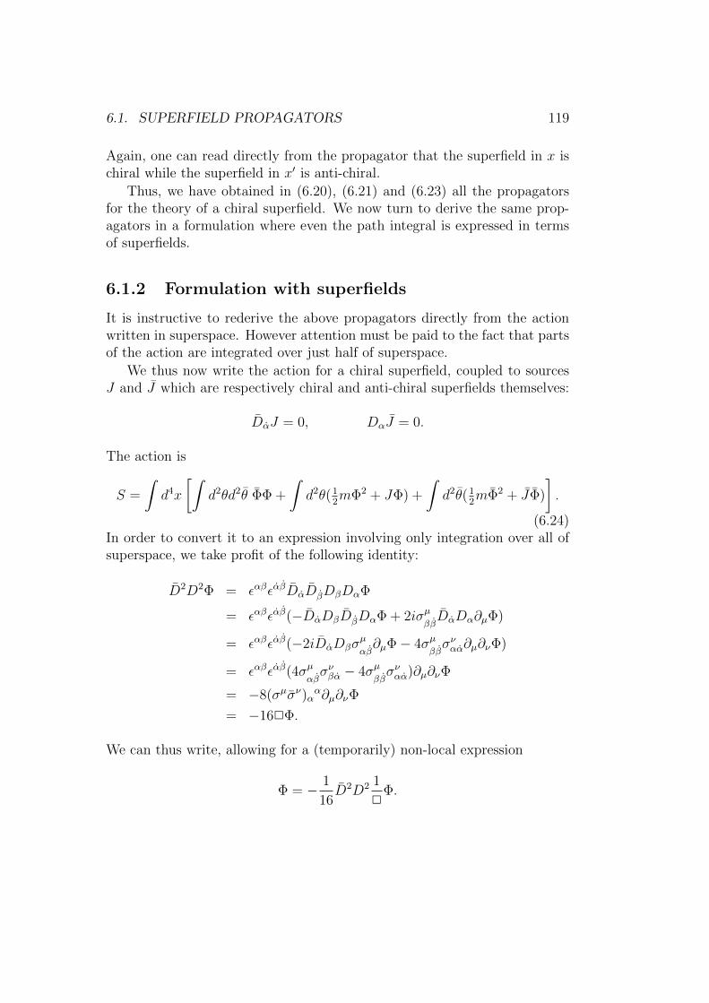
6.1. SUPERFIELD PROPAGATORS 119
Again, one can read directly from the propagator that the superfield in x ischiral while the superfield in x′ is anti-chiral.
Thus, we have obtained in (6.20), (6.21) and (6.23) all the propagatorsfor the theory of a chiral superfield. We now turn to derive the same prop-agators in a formulation where even the path integral is expressed in termsof superfields.
6.1.2 Formulation with superfields
It is instructive to rederive the above propagators directly from the actionwritten in superspace. However attention must be paid to the fact that partsof the action are integrated over just half of superspace.
We thus now write the action for a chiral superfield, coupled to sourcesJ and J which are respectively chiral and anti-chiral superfields themselves:
DαJ = 0, DαJ = 0.
The action is
S =
∫d4x
[∫d2θd2θ ΦΦ +
∫d2θ(1
2mΦ2 + JΦ) +
∫d2θ(1
2mΦ2 + JΦ)
].
(6.24)In order to convert it to an expression involving only integration over all ofsuperspace, we take profit of the following identity:
D2D2Φ = εαβεαβDαDβDβDαΦ
= εαβεαβ(−DαDβDβDαΦ + 2iσµββDαDα∂µΦ)
= εαβεαβ(−2iDαDβσµ
αβ∂µΦ− 4σµ
ββσναα∂µ∂νΦ)
= εαβεαβ(4σµαβσνβα − 4σµ
ββσναα)∂µ∂νΦ
= −8(σµσν)αα∂µ∂νΦ
= −162Φ.
We can thus write, allowing for a (temporarily) non-local expression
Φ = − 1
16D2D2 1
2Φ.

120 CHAPTER 6. RADIATIVE CORRECTIONS
Now we can use the familiar substitution D2 = −4∫d2θ to eventually write
S =
∫d4xd2θd2θ
[ΦΦ +
1
8mΦ
D2
2Φ +
1
8mΦ
D2
2Φ +
1
4ΦD2
2J +
1
4ΦD2
2J
].
(6.25)Using matrices, this is
S =
∫d4xd2θd2θ
[1
2( Φ Φ )
(mD2
421
1 mD2
42
)(ΦΦ
)+ ( Φ Φ )
(D2
42J
D2
42J
)].
(6.26)The kinetic matrix and its inverse are thus
K =
(mD2
421
1 mD2
42
)⇒ K−1 =
2
−2−m2
(mD2
42−1
−1 mD2
42
). (6.27)
We have used for instance that m2D2D2
1622 = −m2
2on anti-chiral superfields.
Hence, if we define
eiW (J,J) =
∫[DΦ]eiS(Φ,Φ,J,J),
we obtain by performing the Gaussian integration
W = −∫d4xd2θd2θ
1
2
(D2
42J D2
42J) 2
−2−m2
(mD2
42−1
−1 mD2
42
)(D2
42J
D2
42J
)= −
∫d4xd2θd2θ
1
2
(D2
42J D2
42J) 1
−2−m2
(−mJ − 1
4D2J
−14D2J −mJ
)=
∫d4xd2θd2θ
(−J 1
−2−m2J +
1
2mJ
1
−2−m2
D2
42J
+1
2mJ
1
−2−m2
D2
42J
). (6.28)
=
∫d4x
[∫d2θd2θ
(−J 1
−2−m2J
)+
∫d2θ
1
2mJ
1
−2−m2J +
∫d2θ
1
2mJ
1
−2−m2J
]. (6.29)
We can find the correlation functions for the superfields by taking func-tional derivatives of iW with respect to iJ and iJ . However note that there

6.1. SUPERFIELD PROPAGATORS 121
is a slight subtlety in taking a functional derivative of a chiral superfield. Agood definition is
δ
δΦ(y′, θ′)Φ(y, θ) = δ2(θ− θ′)δ4(y− y′) = −1
4D2δ2(θ− θ′)δ2(θ− θ′)δ4(x− x′).
(6.30)Indeed, applying this rule, we have
δ
δJ ′
∫d4xd2θ ΦJ = −1
4
∫d4xd2θ Φ(y, θ)D2δ2(θ − θ′)δ2(θ − θ′)δ4(x− x′)
=
∫d4xd2θd2θ Φ(y, θ)δ2(θ − θ′)δ2(θ − θ′)δ4(x− x′)
= Φ(y′, θ′).
Using the shorthand Φ′ ≡ Φ(y′, θ′), we then compute the propagators. Thechiral propagator is
〈0|ΦΦ′|0〉 =δ
δiJ
δ
δiJ ′eiW
= −i δδiJ
m1
−2−m2iJ ′
=im
4
1
−2−m2D2δ2(θ − θ′)δ2(θ − θ′)δ4(x− x′),
exactly reproducing (6.20). As for the chiral-to-anti-chiral propagator, weget
〈0|ΦΦ′|0〉 =δ
δiJ
δ
δiJ ′eiW
= iδ
δiJ
(1
−2−m2(−1
4D′
2)iJ ′)
=i
16
1
−2−m2D2D′
2δ2(θ − θ′)δ2(θ − θ′)δ4(x− x′),
again in exact agreement with (6.23).Before going on to compute the radiative corrections, let us perform the
Fourier transform on the spacetime coordinates. (Note that we will notattempt here to also perform a Fourier transform in the G-odd coordinates,though in some instances this could be of interest.)

122 CHAPTER 6. RADIATIVE CORRECTIONS
In momentum space, the propagators read:
〈0|Φ(p, θ, θ)Φ(−p, θ′, θ′)|0〉 =im
4
1
p2 −m2D2δ2(θ − θ′)δ2(θ − θ′), (6.31)
〈0|Φ(p, θ, θ)Φ(−p, θ′, θ′)|0〉 =i
16
1
p2 −m2D2D′
2δ2(θ − θ′)δ2(θ − θ′), (6.32)
where now of course in D and D we have replaced ∂µ by ipµ.
6.2 Some radiative corrections
We are now able to compute quantum radiative corrections, which appearas Feynman diagrams including loops. Before establishing a theorem thatwill constrain such corrections, we will consider radiative corrections to someselected quantities to get a feeling of how supersymmetry and superspacetechniques facilitate such computations.
Let us first compute the corrections to the propagators themselves.A diagram with a loop inserted inside a 〈ΦΦ〉 propagator involves two
cubic vertices of the type ∫d4xd2θ
λ
3Φ3(y, θ). (6.33)
Note that both vertices should be chiral, in order to tie correctly with thechiral superfields at the two ends of the (corrected) propagator.
As usual in perturbative quantum field theory, for instance from the pathintegral formulation, one has to bring down the vertices in the correlationfunction, and integrate over the momentum running in the loop. Going tothe Fourier transform, we obtain for the corrected propagator
1
2
∫d4xeip(x−x
′)〈0|Φ(x, θ, θ)Φ(x′, θ′, θ′)i
∫d4x1d
2θ1λ
3Φ3(x1, θ1, θ1)·
·i∫d4x2d
2θ2λ
3Φ3(x2, θ2, θ2)|0〉 =
= −2λ2
∫d4kd2θ1d
2θ2im
4
1
p2 −m2D2δ2(θ−θ1)δ2(θ−θ1)·
·im4
1
k2 −m2D2
1δ2(θ1−θ2)δ2(θ1−θ2)
im
4
1
(p− k)2 −m2D2
1δ2(θ1−θ2)δ2(θ1−θ2)·
6.2. SOME RADIATIVE CORRECTIONS 123
·im4
1
p2 −m2D′
2δ2(θ2 − θ′)δ2(θ2 − θ′).
We can concentrate on the central part (which actually corresponds to theamputated diagram, i.e. all that we need to compute the corrections). Recallthat δ2(θ1 − θ2) remains as a factor in the internal propagators, and in theexpression above it will appear twice. Hence, since (θ1 − θ2)4 = 0 becauseof the G-odd nature of the superspace coordinates, the whole expressionvanishes and there are no corrections to the 〈ΦΦ〉 propagator.
This result amounts to stating that the mass parameter appearing in thesuperpotential is not renormalized. As we have just seen, this is automaticin superfield language. In components, the same result would be seen as acancellation between two types of one-loop corrections to the scalar prop-agator: a seagull diagram with a scalar loop and a quartic vertex, againsta diagram with a fermionic loop and two Yukawa vertices. The cancella-tion occurs because of the relation between the couplings of the two kinds ofvertices.
A completely similar vanishing result is obtained for the one-loop correc-tion to the 〈ΦΦ〉 propagator.
On the other hand, the 〈ΦΦ〉 propagator is a different story. Let usconsider a one-loop diagram similar to the one considered previously for the〈ΦΦ〉 propagator, however now one vertex is chiral while the other is anti-chiral. As a consequence, the internal propagators are also of 〈ΦΦ〉 type.Let us compute the correction, focusing on the amputated diagram where wehave dropped the two external propagators. After bringing down the verticesand going to Fourier space, we obtain a contribution proportional to
2λλ∗∫d4kd2θ1d
2θ2i
16
1
k2 −m2D2
1D22δ12
i
16
1
(p− k)2 −m2D2
1D22δ12 =
= −2λλ∗∫d4kd2θ1d
2θ21
k2 −m2
1
(p− k)2 −m2e−(θ1σµθ1+θ2σµθ2−2θ1σµθ2)pµ ,
where in the first line we have used the shorthand δ12 = δ2(θ1−θ2)δ2(θ1− θ2)and in the second line we have used the expression appearing in (6.22). Itis easy to convince oneself that the above expression will contain a non-vanishing, logarithmically divergent term proportional to p2 (for instance, bybringing down twice the last term in the exponential). This divergence willbe compensated by a counterterm which contributes to the wave functionrenormalization of the superfield Φ. Indeed, it was expected that such wave

124 CHAPTER 6. RADIATIVE CORRECTIONS
function renormalization would take place. In components, we would expectindeed from, e.g., the action for the scalar multiplet (3.15) non trivial wavefunction renormalization Zφ and Zψ. What supersymmetry tells us is thatthere is a single function (of the couplings) that renormalizes all the fieldsZφ = Zψ 6= 1.
Let us consider other graphs that yield vanshing contributions. For in-stance, take a “tadpole” graph with only one external Φ line, and a loopattached to it. The only vertex is chiral, and the internal line in the loop isnecessarily of 〈ΦΦ〉 type. However it is a two-point function evaluated at thesame point, in particular at θ = θ′, θ = θ′. Since δ2(θ − θ) = (θ − θ)2 = 0,the internal propagator is
〈0|Φ(p, θ, θ)Φ(−p, θ, θ)|0〉 = 0,
it vanishes identically, and so does any tadpole diagram.Next, we can consider the (one particle irreducible) one-loop correction
to the cubic vertex. Since all external lines are chiral, all three vertices arealso chiral, and then all internal propagators are 〈ΦΦ〉 too. The correctionto the amputated graph is proportional to
4λ3
∫d4kd2θ1d
2θ2d2θ3
(im
4
)31
k2 −m2
1
(p− k)2 −m2
1
(k − q)2 −m2·
·D21δ12D
21δ13D
22δ23.
It is now a simple matter to see that
D21δ12D
21δ13D
22δ23 ∝ (θ1 − θ2)2(θ1 − θ3)2(θ2 − θ3)2 = (θ1 − θ2)4(θ2 − θ3)2 = 0.
This means that there are no radiative corrections to the Φ3 vertex. Itimplies that there is no renormalization (at least at one-loop) of the couplingconstant λ. In other words we have that Zλ = 1, in the same way as wealso had Zm = 1. Of course the wave function renormalization affects thenormalization of the vertices and of the physical mass, but supersymmetryimposes that there is no extra “intrinsic” renormalization of the couplingsappearing in the superpotential.
As a last example, we consider quantum loop corrections to the vacuumenergy (which of course is vanishing classically). At one loop they all vanishfor the same reason as tadpoles (they involve a two-point function evaluatedat the same point). At two-loop level we have one potentially non-trivial

6.3. GENERAL RESULTS ON RENORMALIZATION 125
diagram, with two vertices, one chiral and one anti-chiral, and three 〈ΦΦ〉propagators between them. We now integrate over two different loop mo-menta. The contribution is proportional to
4λλ∗∫d4pd4kd2θ1d
2θ2
(i
16
)31
p2 −m2
1
k2 −m2
1
(p+ k)2 −m2·
·D2pD
2pδ12D
2kD
2kδ12D
2−p−kD
2−p−kδ12 =
= 4λλ∗(i
16
)3 ∫d4pd4kd2θ1d
2θ21
p2 −m2
1
k2 −m2
1
(p+ k)2 −m2·
·e−(θ1σµθ1+θ2σµθ2−2θ1σµθ2)(pµ+kµ−pµ−kµ) =
= 4λλ∗(i
16
)3 ∫d4pd4k
1
p2 −m2
1
k2 −m2
1
(p+ k)2 −m2
∫d2θ1d
2θ2 1 = 0.
Thus we see that the vacuum energy is still zero at two-loops. This is reassur-ing since a non-zero vacuum energy would mean that supersymmetry itself isbroken by perturbative quantum corrections. Let us now try to systematizethese results, also to see if supersymmetry is powerful enough to preventcorrections to some quantities at all orders in the perturbative expansion.
6.3 General results on renormalization
In order to derive systematic results on the renormalization of SUSY the-ories, we need to develop some more formalism, eventually leading to (su-per)Feynman rules that will help in considering generic diagrams contributingto radiative corrections.
Let us first recall the theoretical framework in which Feynman rules areusually derived. The trick is to define correlators in the interacting the-ory in terms of correlators of the free theory, as follows (below, we will beschematical and call φ a representative field):
〈φφ . . . 〉int =
∫[Dφ](φφ . . . )eiS0+iSint(φ)
=
∫[Dφ](φφ . . . eiSint(φ))eiS0
= 〈φφ . . . eiSint(φ)〉free,

126 CHAPTER 6. RADIATIVE CORRECTIONS
where S0 is the (quadratic) action of the free theory.
We now recall that in the free theory, where we define
eiW0(J) =
∫[Dφ]eiS0(φ,J),
the correlation functions are evaluated as
〈φ . . . 〉free =
∫[Dφ](φ . . . )eiS0(φ)
=
(δ
δiJ. . .
)∫[Dφ]eiS0(φ,J)
=
(δ
δiJ. . .
)eiW0(J).
Then, we can define the functional W (the generating function for the con-nected Green functions) for the interacting theory as
eiWint(J) =
∫[Dφ]eiS0(φ,J)+iSint(φ) =
∫[Dφ]eiSint(φ)eiS0(φ,J)
= 〈eiSint(φ)〉free = eiSint(δδiJ
)eiW0(J).
The effective action Γ(φcl), i.e. the generating function of the amputated oneparticle irreducible Green functions, is then obtained by taking the Legendretransform of Wint(J), where we substitute φcl = δW
δJ.
In practice, we will compute the correction to a free correlator at nthorder in the couplings by evaluating
〈φ . . . (iSint(φ))n〉free =
(δ
δiJ. . .
)(iSint(
δ
δiJ)
)neiW0(J). (6.34)
When computing contributions to the effective action Γ(φcl), we must insertclassical fields φcl where the amputated external propagators used to be inthe expression above, and then integrate over the position of such insertions(or, in Fourier space, integrate over the external momenta).
Having summarized the general framework for perturbative computationsin quantum field theories, we now apply it to our SUSY field theories.

6.3. GENERAL RESULTS ON RENORMALIZATION 127
6.3.1 Super-Feyman rules
In order to derive Feynman rules for the SUSY field theory of the Wess-Zumino model, we need to see how does the cubic vertex (6.33) enter in theloop graphs.
In particular, referring to (6.34), we will need to evaluate
iSint(δ
δiJ)iJ1iJ2iJ3 = 2i
∫d4xd2θ4 λ
(−D
21
4
)δ14
(−D
22
4
)δ24
(−D
23
4
)δ34
= 2i
∫d4xd2θ4d
2θ4 λ
(−D
21
4
)δ14
(−D
22
4
)δ24δ34.
We have labeled the fields by their spacetime point, we remind that δ12 isa Grassmann Dirac function on all superspace coordinates, and in the lastequality we have traded a D2 for an integral
∫d2θ.
When computing amputated corrections, we should make sure that wedrop a complete propagator for every external line. Such a propagator alwayshas a D2δ corresponding to it. (Eventually, we must replace each externalpropagator with a classical superfield.) Then, we learn that the D2 that wehave eliminated in the expression above has to be the one corresponding toan internal line. As a consequence, the rule must be that for every vertexthere is a D2 acting on all but one of the internal lines.
For stating the Feynman rules, it is thus more convenient to associatethe action of D2 (or D2 for anti-chiral vertices) to the vertices themselvesrather than to (internal) propagators. We use then the Grisaru-Rocek-Siegelpropagators, which are the ones appearing “naked” in W0(J), see (6.28):
〈Φ1Φ2〉GRS =im
p2 −m2
D21
4p2δ12, (6.35)
〈Φ1Φ2〉GRS =i
p2 −m2δ12. (6.36)
Then, in order to compute terms in the effective action:
• For every chiral vertex we associate a factor of 2iλ and a − D2
4acting
on all but one internal (GRS) propagators attached to the vertex.
• For an anti-chiral vertex, we associate a 2iλ∗ and distribute −D2
4on all
but one internal propagators attached to it.

128 CHAPTER 6. RADIATIVE CORRECTIONS
• For both kind of vertices, we integrate over all of superspace∫d2θd2θ.
• We multiply chiral or antichiral superfields where every external lineused to be, and integrate over the external momenta.
• Finally, we integrate over all loop momenta, and take care of the com-binatorial factors.
(As usual, it is very important to remind oneself of the path integral fromwhich the Feynman rules were derived in order to get all factors and signsright in any specific correlator...)
Let us stress that the important point in the Feynman rules above isreally that we integrate over all of superspace at every vertex. The reason isthat this will allow us to integrate by parts any SUSY covariant derivativeat any vertex, thus making it possible to shift the action of D2 and/or D2
from one propagator to another.
6.3.2 Non-renormalization theorem
With this Feynman rules, we can now prove a general theorem on renor-malization. Given the rules above, any contribution to the effective action(we are considering amputated one particle irreducible graphs) will take thefollowing form.
There will be∫d2θd2θ integrations at every vertex, and all propagators
have a (D2)k(D2)lδ12 or a (D2)k(D2)lδ12 factor, where both k and l are either0 or 1.
The fact that we have written the vertices with a∫d2θd2θ integration
allows us, as advertised previously, to perform integrations by parts andmove the D2 and D2 from one propagator to another (of course, distributingthem according to the Leibniz rule).
Suppose now that we choose one specific loop in the graph. By (Grass-mann) partial integrations on every successive vertex along the loop, we canremove all the D2 and D2 to only one of the propagators composing the loop,let us say for definiteness the one between the first two vertices. Noting thatwe can lower the number of SUSY-covariant derivatives by using expressionssuch as D2D2D2 ∝ 2D2, we will eventually arrive at an expression like∫d4θ1d
4θ2 . . . d4θn δ23δ34 . . . δn1(D2)k(D2)lδ12 =
∫d4θ1d
4θ2 δ12(D2)k(D2)lδ12.

6.3. GENERAL RESULTS ON RENORMALIZATION 129
Such an expression is non vanishing if and only if k = l = 1. Indeed, if eitherk or l is larger than 1 then e.g. D4 = 0, while if either k = 0 or l = 0 we willhave e.g. (θ1 − θ2)4 = 0.
Thus in the only case where we have a non-vanishing result, the contri-bution will read∫
d4θ1d4θ2 δ12D
2D2δ12 =
∫d4θ1d
4θ2 δ12(. . . ) =
∫d4θ1 (. . . ).
The end result of this procedure has been to effectively contract the loop toone of its vertices. Importantly, attached to this last vertex we still have afull superspace integral
∫d4θ1 ≡
∫d2θ1d
2θ1. The integrand is a function ofthe momenta, both loop and external (which will generically enter at everyvertex, and appear in the denominator of the propagators), of θ1 and θ1, andof all the other Grassmann variables associated to the other vertices.
We can then repeat the same argument on another remaining loop ofthe effective graph obtained in the previous step. The procedure will go onexactly as before. Eventually, if the graph does not vanish, we will end upnecessarily with a contribution given by an expression like∫
d2θd2θ
∫d4p1 . . . d
4pkd4k1 . . . d
4kn F1(p1, θ, θ) . . . Fk(pk, θ, θ)·
·G(p1, . . . , pk; k1, . . . , kn),
where the graph had originally n loops with their associated momenta ki,while the functions Fi are generic (Fourier transforms of) superfields de-pending on each external momentum pl. The function G encodes all theremaining momentum dependence coming from the (bosonic) denominatorsof the propagators.
Going back to x-space, we see that the typical contribution to the effectiveaction will be∫
d4x1 . . . d4xk
∫d2θd2θ F1(x1, θ, θ) . . . Fk(xk, θ, θ)G(x1, . . . , xk).
This expression can of course be non-local in space-time, but (oddly enough)it is local in the G-odd variables, and it is necessarily integrated over all ofsuperspace. Hence the effective action contains corrections to the d-terms,but not to the f -terms. This is why there is wave-function renormalization
Γ ∝ δΦ
∫d4xd2θd2θ ΦΦ,

130 CHAPTER 6. RADIATIVE CORRECTIONS
but no renormalization of m and λ, which would imply terms like
δm
∫d4xd2θ Φ2 and δλ
∫d4xd2θ Φ3.
Also, the vacuum energy cannot receive corrections, since that would implya contribution to Γ with no external superfields, that is with all Fi = 1, butthen the Grassmann integral gives trivially zero. The vacuum energy thenstays zero at any order in perturbation theory.
This latter result is of course very important, it means that supersymme-try cannot be broken by perturbative quantum effects. As we will see in thenext chapter, the only option to break supersymmetry spontaneously will beeither at tree level, or due to non-perturbative effects.
It is a simple exercise to revisit the previous examples of radiative cor-rections using the Feynman rules of the present section.
The one-loop correction to the term with two external chiral superfields Φin the effective action will be computed by writing the same diagram, puttinga D2 on both internal 〈ΦΦ〉 lines, and also a D2 on each line from both ver-tices. Integrating by parts, we end up (being careful to which Grassmanncoordinates the supercovariant derivatives act upon) with an expression con-taining
∫d2θd2θΦ(x, θ)2 which gives just a boundary term in the effective
action. An exactly similar argument can be given for all one-loop diagramswith only chiral external legs, thus proving that there are no corrections tothe superpotential in the quantum effective action.
Instead, the one-loop correction to the term with Φ and Φ external legscan be evaluated by putting a D2 on one line from the chiral vertex, anda D2 on the same line (or the other, and then integrating by parts) fromthe anti-chiral vertex. Here we end up with a contribution to the effectiveaction proportional to
∫d2θd2θΦ(x, θ)Φ(x, θ), which is just the familiar wave-
function renormalization.Finally, the two loop vacuum energy diagram is evaluated by distributing
a D2 and a D2 on two of the three lines. Then one of the two loops canbe eliminated, leaving a one-loop vacuum diagram with a propagator withD2D2 acting on it. This leads to
∫d2θd2θ1 = 0 as before.
More details and other examples can be found in M. T. Grisaru, W. Siegeland M. Rocek, “Improved Methods For Supergraphs,” Nucl. Phys. B 159(1979) 429, and in chapter 6 of the book/review S. J. Gates, M. T. Grisaru,M. Rocek and W. Siegel, “Superspace, or one thousand and one lessons insupersymmetry,” Front. Phys. 58 (1983) 1 [arXiv:hep-th/0108200].

6.4. RENORMALIZATION OF THE REAL SUPERFIELD 131
6.4 Renormalization of the real superfield
All the above discussion and theorems concerned the theory of a single chiralsuperfield. The generalization to a theory with many different chiral super-fields is obvious and straightforward. However extending the formalism toreal (vector) superfields is more complicated, and we will not review it here.
Let us only remark the following. Corrections to the quantum effectiveaction must be written as manifestly SUSY and gauge invariant terms. Henceany term δL will have to be either a d-term or an f -term. In particular,the renormalization of the gauge coupling is related to the wave-functionrenormalization of the fields in V . This is not a real surprise as this isalready the case in non-supersymmetric gauge theories after all.
To see this in more detail, couple first V to matter fields Φ in somerepresentation. Then the d-term∫
d2θd2θ Φe2gV Φ
gets corrections, which however must be of the same form as the kinetic termitself, so that
Leff ∝ ZΦ
∫d2θd2θ Φe2gV Φ,
where ZΦ = 1 + δΦ and δΦ is really the coefficient extracted from the loopcomputation.
It is important to note that we cannot have a generic
Leff ∝ ZΦ
∫d2θd2θ Φe2ZggZ
1/2V V Φ,
because that would mean that we would have generated from loop diagramsa correction term like
δL ∝∫d2θd2θ Φe2gV V Φ,
which is not gauge invariant.In other words, since we can rescale g into V , we really need to have only
one independent renormalization function, which we will choose to be ZV .This is purely a consequence of gauge symmetry, and not of supersymmetry.Supersymmetry just tells us that the gaugino undergoes the same wave-function renormalization as the gauge field.

132 CHAPTER 6. RADIATIVE CORRECTIONS
A similar argument, which applies also to pure (non-abelian) gauge the-ories is as follows. The gaugino superfield Wα will be renormalized by thesame function as the real superfield V . This implies that the non-abelianfield strength will be renormalized as
Fµν → Z1/2V Fµν .
Now, Fµν contains a quadratic term g[Aµ, Aν ] which has to be renormalizedin the same way as the term linear in Aµ, otherwise, again, that would meannon-gauge invariant corrections in the effective action. We thus obtain againthat
ZgZ1/2V = 1.
Note that ZV 6= 1 means that there are corrections
δL ∝ δV
∫d2θ trWαWα + c.c.
This seems to contradict the theorem that the terms generated in the effectiveaction should all be of the form
∫d2θd2θ (to be honest, we proved the theorem
only in the presence of chiral superfields but it is indeed true also when realsuperfields are present).
However recall that
trWαWα ∝ D2trWαe−VDαeV ,
and thus we can rewrite
δL ∝ δV
∫d2θd2θ trWαe−VDαe
V + c.c.
which gives a SUSY and gauge invariant term in the effective action (afterintegrating over spacetime). The truth is that, as we had already noticed,the gauge kinetic term is only a “fake” f -term since it can be rewritten as aperfectly fine local d-term.
Hence, Zg 6= 1 and the gauge coupling in SUSY gauge theories indeedruns. This is a welcome feature, and it was expected since, for instance,in SU(N) super-Yang-Mills theory it is quite easy to compute the one-loopbeta function in component fields (it is just like QCD with one adjoint Weylfermion), finding
β(g) ≡ dg
d log µ= − 3N
16π2g3.

6.5. HOLOMORPHY AND NON-RENORMALIZATION 133
For completeness, we list here the beta function for SU(Nc) SQCD withNf flavors. Extracting it from known computations involving the componentfields is also quite straightforward, though one needs to know the contributionto the beta function of QCD from charged scalars. [This information canbe retreived e.g. in chapter 16 of M. E. Peskin and D. V. Schroeder, “AnIntroduction To Quantum Field Theory,” Addison-Wesley (1995).] The one-loop result is
β(g) = − 1
16π2(3Nc −Nf )g
3. (6.37)
We see that there is a large range of values of Nf such that the theory isasymptotically free (β < 0).
6.5 Holomorphy and non-renormalization
As a last comment on renormalization properties of SUSY field theories,let us argue for the non-renormalization of the superpotential W (Φ) in acompletely different way. This approach is mainly due to Seiberg.
Let us consider again a Wess-Zumino model of one chiral superfield Φwith
W (Φ) =1
2mΦ2 +
1
3λΦ3. (6.38)
Recall that we have symmetries acting on the fields. Here we have essentiallytwo U(1)s: one rotating each physical component of Φ. At the level of thesuperfield, we have an R-symmetry and an axial-like symmetry:
U(1)R : φ→ φ, ψ → e−iαψ (θ → eiαθ)
U(1)Φ : φ→ eiαφ, ψ → eiαψ.
The superpotential breaks explicitly both of these symmetries.Let us now remark that also the coupling constants m and λ enter holo-
morphically in the superpotential W . We could thus promote them to back-ground (moduli) chiral superfields, so that the physical couplings are actuallythe vacuum expectation values of these fields whose dynamics is frozen bysome other means (e.g., their kinetic term is suppressed). Now, it becomespossible to assign charges under the global symmetries to these superfieldsso that the superpotential is invariant, i.e. it should have R-charge 2 andΦ charge 0. If we keep calling the background superfields by the constants

134 CHAPTER 6. RADIATIVE CORRECTIONS
they are related to, the transformation laws that we need to impose are thefollowing:
U(1)R : m→ e2iαm, λ→ e2iαλ
U(1)Φ : m→ e−2iαm, λ→ e−3iαλ.
Now since W (Φ,m, λ) preserves both U(1)s (which are not anomalous sincethere are no gauge symmetries around), then the effective superpotential Weff
(that is, the part of the effective action that cannot be written as a d-term)must also preserve them, and because supersymmetry is also preserved Weff
must be a holomorphic function of Φ, m and λ.These requirements imply that
Weff =1
2mΦ2f
(λΦ
m
), (6.39)
where λΦm
is the only chargeless holomorphic combination of the superfields,and f(z) is a holomorphic function.
Once we assume that the background superfields have frozen to theirVEVs, we can now analyze various limits in order to constrain the form off(z). When λ = 0 the theory is free, and we should find no corrections tothe classical action. Hence
Weff(λ = 0) = Wtree(λ = 0) =1
2mΦ2.
This implies that f(0) = 1.If we Taylor expand f so that
f(z) = 1 + a1z + a2z2 + . . . ,
with ai some numerical coefficients, we get for the effective superpotential
Weff =1
2mΦ2 +
1
2a1λΦ3 +
1
2a2λ2
mΦ4 +O
(λ3
m2
). (6.40)
We can then scale both λ and m to zero in such a way that m ∝ λ2 → 0.The first two terms scale to zero, while the third is constant and the higherorder ones diverge. This is clearly impossible for a theory with Wtree → 0.Hence we understand that a2 = a3 = · · · = 0 and f = 1 + a1t.

6.5. HOLOMORPHY AND NON-RENORMALIZATION 135
Another way to see this is the following. The coefficient an multipliesa term like λn
mn−1 Φn+2. Such a term must arise from a graph with n chiralvertices and n+ 2 external lines. It is easy to see that only tree-level graphscan accomodate that, and they are not one-particle irreducible. Hence theycannot contribute to the effective action and such corrections cannot arise,i.e. all their coefficient must vanish.
Finally, the O(λ) term in Weff cannot be anything else than the vertex inWtree. Thus, we have proven that
Weff = Wtree.
This is entirely equivalent to the perturbative non-renormalization theoremof the superpotential Wtree.
Actually, in the present context we can even extend this result to non-perturbative effects. If their contribution is to be holomorphic in λ, then suchterms will be proportional to, say, e−1/λ. However if λ approaches 0 from thenegative real axis, the non-perturbative contribution would explode, whichmakes no sense for a vanishingly small coupling. Hence holomorphy rulesout also non-perturbative corrections to the effective superpotential, at leastin theories of chiral superfields only.
Let us mention as a last remark that when (asymptotically free) gaugetheories are also in the game, there is a class of non-perturbative correctionsthat are possible, and indeed can be shown to arise in many cases. Thereason is that because of dimensional transmutation, one can trade the run-ning gauge coupling g for a holomorphic scale which is defined in terms thecomplexified coupling τ given in (4.55) by
Λ = µe− 8π2
b0τ(µ)
= µe− 8π2
b0g2(µ)
+i Θb0 . (6.41)
It is this Λ that can be considered as a background chiral superfield as in theargument above, and thus holomorphy does not prevent it from entering inthe effective superpotential Weff . Furthermore, Λ goes to zero when the gaugecoupling is sent to zero. The perturbative non-renormalization theorem is notcontradicted because corrections proportional to some (necessarily positive)power of Λ are of course non-perturbative in the gauge coupling g.

136 CHAPTER 6. RADIATIVE CORRECTIONS

Chapter 7
Supersymmetry breaking
Supersymmetry breaking is an issue that must be addressed since in the realworld supersymmetry is broken. Indeed, there is no degeneracy betweenboson and fermion masses. More precisely, since we established that theminimally supersymmetric version of the Standard Model is the MSSM, it isthen an experimental fact that the masses of all the superpartners are notlighter than the Electro-weak scale, otherwise they would have been alreadyobserved in the previous generation of accelerators.
Yet, for supersymmetry to be really helpful in curing the hierarchy prob-lem, it must be restored at some intermediate scale between MEW ∼ 100GeV and MGUT ∼ 1016 GeV. Usually, it is expected that SUSY is restoredclose to MEW , so as to maintain (and possibly explain) the hierarchy betweenMEW and MGUT .
How do we cook up then a theory which is supersymmetric at high en-ergies but is not supersymmetric at lower energies? Supersymmetry will bebroken by some dimensionful quantity MSUSY , so that for E > MSUSY thetheory behaves supersymmetrically, while for E < MSUSY it will not (e.g.,there will be mass splittings among superpartners).
There are two ways in which we can introduce such a dimensionful break-ing:
i) Spontaneous SUSY breaking: The theory as a whole preserves SUSY,but its vacuum does not. Namely, there will be a field acquiring a VEV〈ϕ〉 ∼MSUSY such that SUSY is broken.
ii) Explicit (soft) SUSY breaking: The Lagrangian of the theory containsterms which do not preserve SUSY. However it is assumed that are
137

138 CHAPTER 7. SUPERSYMMETRY BREAKING
present only those terms (dubbed soft) that preserve the high energybehavior of SUSY (i.e. the UV cancellations). These soft terms alwayscorrespond to dimensionful parameters.
We will actually see that it is possible to treat case ii) as a specific limit ofcase i).
In the rest of this chapter we concentrate on spontaneous SUSY breaking,which is also the most natural option, since in some sense it requires thetheory itself to predict that SUSY is broken.
7.1 Spontaneous SUSY breaking
We have seen at the very beginning, in Chapter 2, that the first consequenceof the SUSY algebra is that a SUSY ground state must have vanishing energy.Indeed, to repeat the argument, the superalgebra
Qα, Qα = 2σµααPµ
implies that, for any state and thus also for a ground state |Ω〉
δαα〈Ω|Qα, Qα|Ω〉 =∑α
‖Qα|Ω〉‖2 +∑α
‖Qα|Ω〉‖2 ≥ 0
= 4E‖|Ω〉‖2,
so that E = 0 if and only if Qα|Ω〉 = 0 = Qα|Ω〉. What is most importanthere, is that it is also true that as soon as E > 0, then we know that theremust exist an α or an α such that Qα|Ω〉 6= 0 or Qα|Ω〉 6= 0. In other words,the vacuum |Ω〉 is not SUSY invariant. Hence, SUSY is broken spontaneously.
This means that the vacuum energy E is an order parameter for brokenSUSY: whenever E > 0 SUSY is broken, while if E = 0 SUSY is preserved.This observation is in line with the fact that spontaneous breaking of globalsymmetries is always associated to an order parameter. Below, we turn tothe Lagrangian version of this consequence of broken SUSY.
7.1.1 Vacuum energy and f- and d-terms
We can restate the above observation in more detail and at the classical levelconsidering the most general SUSY theory with gauge fields and matter. The

7.1. SPONTANEOUS SUSY BREAKING 139
Lagrangian is
L =
∫d2θd2θ
∑r
Φre2gVaT
(r)a Φr +
∫d2θ W (Φr) +
∫d2θ W (Φr)
−τ8
∫d2θ trWαWα −
τ
8
∗∫d2θ tr WαW α.
The only contribution to the vacuum energy, at the classical level at least,comes from the scalar potential:
V(φr, φ∗r) =
∑r
(∂W
∂φr
)i
(∂W
∂φr
)i+
1
2g2∑a
(∑r
φ∗riT(r)a
i
jφjr
)2
≡∑r
f ∗rifir +
1
2
∑a
dada,
where we write derivatives with respect to the scalar fields, to denote thefact that the expression is a function of them. We have V = 0, and thusvanishing classical energy, if and only if fr = 0 and da = 0 for all values of rand a.
Indeed, consider a vacuum state of such a theory. In order for the vacuumto preserve Poincare symmetry, the only fields which can acquire a VEVmust be Lorentz scalars. Moreover the VEV must be constant throughoutspacetime. Consider now the SUSY variations of the fermions in such avacuum. (The ones for the bosons are automatically vanishing since thefermions are set to zero.) For the matter fields we have
δψir =√
2εf ir,
while in the gauge sector we have
δλa = iεda.
Hence a vacuum configuration is SUSY invariant, i.e. the variations of all thefields are zero, if and only if fr = 0 and da = 0, which as we have just seenimplies that the potential vanishes, V = 0.
We have thus demonstrated that V is an order parameter for SUSY break-ing, playing at the classical level the role that E was playing at the quantumlevel.

140 CHAPTER 7. SUPERSYMMETRY BREAKING
7.1.2 The SUSY breaking vacuum and the goldstino
For a SUSY preserving vacuum, we can content ourselves with solving the“first order” conditions f = 0 and d = 0. Since the potential is positivesemi-definite, V ≥ 0, if we find a state with V = 0 we are ensured that it isa global minimum of V , in particular it is a stationary point.
For a vacuum which is not SUSY, there are no short-cuts and we mustfind a stationary point of the potential V by computing its first derivativeand setting it to zero:
dV = 0 ⇔ ∂V∂φir
= 0, ∀r, i. (7.1)
For simplicity, let us suppress from now on the index r of the representation,we can just group together all the irreducible representations into a singlereducible one.
Then, given the potential
V =∂W
∂φi∂W
∂φi+
1
2g2∑a
(φ∗iTa
ijφ
j)2,
we obtain for its first derivative
∂V∂φi
=∂2W
∂φi∂φj∂W
∂φj+ g2
∑a
(φ∗jTa
jkφ
k)φ∗l Ta
li
= − ∂2W
∂φi∂φjf j − g
∑a
φ∗l Talida,
where we have used (5.12) and (5.13). We thus have the condition for anextremum of the potential:
dV = 0 ⇔ ∂2W
∂φi∂φjf j + gφ∗l Ta
lida = 0, (7.2)
where now it is intended that there is a sum also over the repeated a indices.Of course, one should now check that the extremum that has been found
is really a minimum, at least a local one. For instance, one should computethe mass matrix for the scalars around that minimum, and check that all theeigenvalues m2 are positive. We will show an example of such a procedurefor an example in the following.

7.1. SPONTANEOUS SUSY BREAKING 141
By considering instead the mass matrix for the fermions, there is a niceconsequence of the existence of such an extremum that can be extracted fromthe above expression for dV = 0.
Consider the mass matrix of the fermions of the theory, including theYukawa-like interactions where we suppose that the scalars are frozen attheir extremum value:
Lmass,fermions = ig√
2φ∗iTaijλaψ
j − 1
2
∂2W
∂φi∂φjψiψj + c.c. (7.3)
= −1
2( ψi λa )
(∂2W∂φi∂φj
− ig√2φ∗l Tb
li
− ig√2φ∗kTa
kj 0
)(ψj
λb
)+ c.c.
Before jumping to any conclusion, we need the following last bit of in-formation. The superpotential is gauge invariant, which means that under agauge transformation
δαφi = αaTa
ijφ
j
it should stay invariant, δαW = 0. This translates into
0 =∂W
∂φiδαφ
i = −f ∗i αaTaijφj,
so that invariance of W under any gauge transformation imposes a relationbetween the f -terms:
φ∗iTaijf
j = 0. (7.4)
This relation is always true, in particular for values of the scalar fields thatcorrespond to an extremum of the potential. Hence, summing together theconditions (7.2) and (7.4), we see that at an extremum dV = 0 the fermionicmass matrix (
∂2W∂φi∂φj
− ig√2φ∗l Ta
lj
− ig√2φ∗kTb
ki 0
)has at least one zero eigenvalue, with eigenvector given by(
f i
i√
2da
). (7.5)
This eigenvector is non-trivial only in a SUSY breaking vacuum (i.e. whenf i and da are not all zero). Hence we have proven the Goldstone theorem for

142 CHAPTER 7. SUPERSYMMETRY BREAKING
broken supersymmetry: a vacuum spontaneously breaking SUSY necessarilypossesses a massless fermionic particle in the spectrum. This particle isusually called the Goldstone fermion of broken SUSY, or more familiarly thegoldstino.
We thus see that supersymmetry in this respect is much similar to anyother continuous global symmetry. Indeed, the Goldstone theorem dictatesthat for any spontaneously broken (bosonic) global symmetry there must bea massless boson in the spectrum, the Goldstone boson.
We should point out that there is also a more general proof of the Gold-stone theorem for broken SUSY, which is not based on an explicit classicalLagrangian, but on the properties of the supercurrent. This more generalproof establishes the presence of a goldstino even if SUSY is broken in astrongly coupled phase of a given theory, where classical arguments may notapply.
7.1.3 The supertrace theorem
Let us now restrict to a theory of chiral superfields only, in order to avoid tooinvolved formulas. We would like to consider the mass spectrum in a genericvacuum, where supersymmetry is possibly broken.
We have already seen in the previous subsection that the fermionic massmatrix is given by
Lfmass = −12ψiMf
ijψj + c.c.,
where
Mfij =
∂2W
∂φi∂φj≡ ∂i∂jW. (7.6)
The physical squared masses of the fermions (i.e. the real poles in the tree-level fermionic propagators) will be given by the eigenvalues of
MfijMf∗jk ≡ (M2
f )ki = ∂i∂jW∂∂kW ,
where we have defined ∂ı ≡ ∂∂φi
and the sum over the index j is intended.
The full squared mass matrix over all of the fermionic degrees of freedom (ofboth chiralities) is thus
M2f =
(∂i∂jW∂∂kW 0
0 ∂ı∂W∂j∂kW
). (7.7)

7.1. SPONTANEOUS SUSY BREAKING 143
Consider now the scalar mass matrix. It is obtained by expanding thescalar potential to quadratic order around the vacuum values of the scalars.We get:
Lbmass = −∂iW∂ıW
= −(∂iW + ∂i∂jWφj + 12∂i∂j∂kWφjφk) ·
·(∂ıW + ∂ı∂lWφ∗l + 12∂ı∂l∂mWφ∗l φ
∗m).
In the above expression, we define the fields φi as their fluctuation aroundthe minimal value, while the derivatives of the superpotential are evaluatedat the vacuum values. Note that for a renormalizable superpotential theexpansion indeed stops at quadratic order, while in a more generic situationit can go on, but since we are interested only in quadratic terms we do notneed the higher order terms anyway.
Supposing that we expand around an extremum, and neglecting the con-stant vacuum energy term, the quadratic mass terms are hence given by
Lbmass = −∂i∂jW∂ı∂kWφjφ∗k − 12∂i∂j∂kW∂ıWφjφk − 1
2∂ı∂∂kW∂iWφ∗jφ
∗k.
(7.8)Eventually, we have
Lbmass = −12( φ∗i φi )(M2
b)ij
(φj
φ∗j
),
with
(M2b)ij =
(∂ı∂kW∂j∂kW −∂ı∂∂kWf ∗k−∂i∂j∂kWfk ∂i∂kW∂∂kW
). (7.9)
There are two immediate consequence that one can gather by comparing(7.7) and (7.9). First of all, there will be mass splittings in the eigenvaluesof M2
f and M2b if and only if f 6= 0. Indeed, otherwise the two matrices
are identical, in agreement with the fact that when SUSY is unbroken thespectrum of fermions and bosons is degenerate.
However also in a broken SUSY vacuum there is a relation between thetwo mass spectra. We can compute the sum of the eigenvalues by takingthe trace of the two mass matrices. For the fermionic one, which is blockdiagonal, we get
trM2f = 2
∑i∈f
m2i = 2∂i∂jW∂ı∂W ,

144 CHAPTER 7. SUPERSYMMETRY BREAKING
(the factor of 2 in front of the sum corresponds to the helicities of eachfermion), and for the bosonic one we obtain
trM2b =
∑i∈b
m2i = 2∂i∂jW∂ı∂W ,
which is the same since the two matrices only differ by off-diagonal elements.The important consequence is that the supertrace, that is the trace weighted
according to the statistics, vanishes:
StrM2 =∑i∈b
m2i − 2
∑i∈f
m2i = 0. (7.10)
This important result generalizes straightforwardly to theories with gaugefields.
It means that when SUSY is broken in such a classical fashion, the massesof the previously degenerate superpartners are split around an average value,which is related to the unbroken (SUSY) mass.
This fact, which is a consequence of the theory being supersymmetric,is unsatisfactory because it leads to strong constraints on the spectrum ofsuperpartners, which are not met phenomenologically. For instance, for everyquark there should be at least a real component of the squark superpartnerwhich would be lighter: this is clearly not observed.
Does this mean that spontaneous SUSY breaking is not viable for theMSSM? In reality, the “supertrace theorem” just means that SUSY is notspontaneously broken at tree level (i.e. classically) within the MSSM itself.Indeed, a way out for this problem is to assume that SUSY breaking is nota tree level phenomenon, or that it happens in a separate, hidden sector.In both cases, or even better in a combination of these two possibilities,SUSY breaking is transmitted to the MSSM by quantum corrections. At thequantum level, there are effective corrections to the kinetic terms (e.g. wavefunction renormalization) such that the supertrace theorem can be violated,and sizable masses for all the superpartners can be generated. We will comeback briefly on this issue when discussing the soft terms.
7.2 Examples of SUSY breaking theories
The supertrace theorem notwithstanding, and for the reasons just mentioned,it is still relevant to review models of tree level spontaneous SUSY breaking.

7.2. EXAMPLES OF SUSY BREAKING THEORIES 145
We will discuss below the two archetypal models, one of d-term breaking andthe other of f -term breaking.
7.2.1 d-term breaking: Fayet-Iliopoulos model
The Fayet-Iliopoulos model is a very simple model, where one essentiallyplays the f -terms and the d-terms against each other.
In its simplest incarnation, it is the SQED model that we had alreadyconsidered previously, with a mass term for the quark superfields and theaddition of the FI term (4.58). All in all the model is described by
L =
∫d2θd2θ
(Φe2gV Φ + Φe−2gV ¯Φ
)+
∫d2θ mΦΦ +
∫d2θ m∗Φ ¯Φ
−1
4
∫d2θ WαWα −
1
4
∫d2θ WαW α +
∫d2θd2θ 2ξgV. (7.11)
Recall that the last term is gauge invariant because V is an abelian realsuperfield, and that ξ is a real parameter.
The potential is given by
−V = gd(φ∗φ− φφ∗) + ff ∗ + f f ∗ + (mφf +mφf + c.c.) + 12d2 + gξd.
Solving for the auxiliary fields d, f and f , we have
f ∗ = −mφf ∗ = −mφd = −g(φ∗φ− φφ∗ + ξ), (7.12)
so that the potential for the scalars becomes
V = 12g2(|φ|2 − |φ|2 + ξ)2 + |m|2(|φ|2 + |φ|2). (7.13)
It is clear that we will not find SUSY vacua. Indeed, f = 0 = f impliesthat the scalars themselves must vanish, φ = 0 = φ, while, when ξ 6= 0,the condition d = 0 would imply that either φ or φ must be non zero. It isthen impossible to set to zero all the right hand sides of (7.12), and SUSY isbroken.
To find the non SUSY vacuum, we extremize the potential V :
∂φV = g2(|φ|2 − |φ|2 + ξ)φ∗ + |m|2φ∗,∂φV = g2(|φ|2 − |φ|2 − ξ)φ∗ + |m|2φ∗.

146 CHAPTER 7. SUPERSYMMETRY BREAKING
We see that we have a vacuum at φ = 0 = φ. Assuming without loss of
generality that ξ > 0, we also have a vacuum for φ = 0 and |φ|2 = ξ − |m|2
g2 ,
which exists only when |m|2 < g2ξ. When this inequality is satisfied, it is asimple matter to show that the vacuum with a non trivial scalar VEV is thestable one, while the other at the origin becomes unstable.
When the stable vacuum is at the origin, we have φ = 0 = φ which impliesthat
f = 0 = f and d = −gξ 6= 0,
the vacuum energy beingV = 1
2g2ξ2.
This is pure d-term SUSY breaking, and it is rather easy to see that thegoldstino in this case is just the photino λ, the only massless fermion aroundin this vacuum.
When the stable vacuum is the one with φ = 0 and |φ|2 = ξ − |m|2g2 ,
we see that both f 6= 0 and d 6= 0. This situation becomes one of pure
f -term SUSY breaking only in the limit ξ |m|2g2 . Then the role of the
goldstino is essentially played by ψ. (Indeed, ψ and λ become massive due tothe super-Brout-Englert-Higgs mechanism: φ '
√ξ breaks the U(1) gauge
symmetry and through the Yukawa couplings gives a fermionic Dirac massterm Lfm = −ig
√2ξψλ, while ψ remains massless.)
7.2.2 f-term breaking: O’Raifeartaigh model
The model first proposed by O’Raifeartaigh is composed of chiral superfieldsonly. The idea here is to have a superpotential W such that one cannot setto zero all the f -terms. Of course this means that W is not generic.
A superpotential that works is the following. There must be three differ-ent chiral superfields:
W = hX(Φ21 − µ2) +mΦ1Φ2. (7.14)
If we call X (by a slight abuse of notation), φ1 and φ2 the lowest componentsof the respective superfields, then the f -term equations give the followingconditions
−f ∗X = h(φ21 − µ2), (7.15)
−f ∗1 = 2hXφ1 +mφ2, (7.16)
−f ∗2 = mφ1. (7.17)

7.2. EXAMPLES OF SUSY BREAKING THEORIES 147
It is evident that one cannot set fX = 0 and f2 = 0 simultaneously, as soonas µ 6= 0. Let us look then at the scalar potential
V = |h|2|φ21 − µ2|2 + |2hXφ1 +mφ2|2 + |m|2|φ1|2. (7.18)
It will have an extremum dV = 0 if
2h∗φ∗1(2hXφ1 +mφ2) = 0,
2|h|2(φ21 − µ2)φ∗1 + 2h∗X∗(2hXφ1 +mφ2) + |m|2φ1 = 0,
m∗(2hXφ1 +mφ2) = 0.
From the third equation we see that we can solve for φ2:
φ2 = −2h
mXφ1. (7.19)
Then the first equation is also satisfied, and we are left with the second one,simplified as
2|h|2|φ1|2φ1 − 2|h|2µ2φ∗1 + |m|2φ1 = 0. (7.20)
Note that by rotations of X, Φ1 and Φ2 we can set for simplicity all constantsto be real and positive.
It is evident that (7.20) has always the solution φ1 = 0. At this vacuum,we have also φ2 = 0 while X is undetermined.
Otherwise, if φ1 6= 0, since we have chosen all constants to be real andpositive, we see that also φ1 has to be real, and has to satisfy
2h2φ21 = 2h2µ2 −m2.
Thus this alternative vacuum exists only when 2h2µ2 ≥ m2. When thisinequality is satisfied, the latter vacuum is the stable one. Otherwise, theonly vacuum is the one at the origin φ1 = φ2 = 0. From now on we setourselves in this vacuum, and suppose that it is stable.
The f -terms are
f1 = f2 = 0, f ∗X = hµ2,
so that the vacuum energy is given by
Vvac = |hµ2|2.

148 CHAPTER 7. SUPERSYMMETRY BREAKING
What is puzzling about this vacuum is that there is actually a complex planeof vacua, parameterized by 〈X〉. This is a usual fact for SUSY vacua, butit is rather unusual for SUSY breaking vacua. In non-SUSY theories, suchdegeneracies are expected to be lifted by quantum corrections.
Actually, the whole X supermultiplet is massless in the non-SUSY groundstates. The fermionic component, ψX , is the goldstino, and then it has a goodreason to be massless. The same can be said about the phase of the complexscalar X, since as we will argue below it corresponds to the Goldstone bosonfor broken R-symmetry. However the modulus |X| has no specific reasonat all to stay massless. Presumably, it should acquire a mass because ofquantum corrections in the non-SUSY vacuum.
Before considering this issue, and actually in order to do so, we firstcompute the spectrum of masses in a vacuum parameterized by the VEV ofX.
We start by considering the fermionic mass matrix, computed thus in thevacuum with φ1 = φ2 = 0 and X arbitrary:
Lfmass = −1
2( ψX ψ1 ψ2 )
0 0 00 2hX m0 m 0
ψXψ1
ψ2
+ c.c., (7.21)
so that
M2f =
0 0 00 4|hX|2 + |m|2 2hXm∗
0 2h∗X∗m |m|2
. (7.22)
There is a vanishing eigenvalue (for ψX), while the other two are given by
m2f,± = |m|2 + 2|hX|2 ±
√4|hXm|2 + 4|hX|4
=(|hX| ±
√|m|2 + |hX|2
)2
. (7.23)
As for the bosons, we use the general expression (7.9), and obtain
Lbmass = −12v†M2
bv, (7.24)
with
v† = ( X φ1 φ2 X∗ φ∗1 φ∗2 ), (7.25)
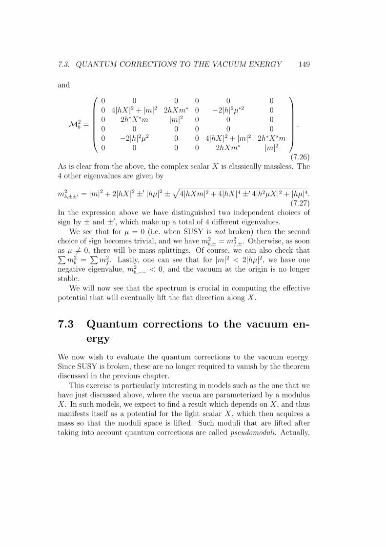
7.3. QUANTUM CORRECTIONS TO THE VACUUM ENERGY 149
and
M2b =
0 0 0 0 0 00 4|hX|2 + |m|2 2hXm∗ 0 −2|h|2µ∗2 00 2h∗X∗m |m|2 0 0 00 0 0 0 0 00 −2|h|2µ2 0 0 4|hX|2 + |m|2 2h∗X∗m0 0 0 0 2hXm∗ |m|2
.
(7.26)As is clear from the above, the complex scalar X is classically massless. The4 other eigenvalues are given by
m2b,±±′ = |m|2 + 2|hX|2 ±′ |hµ|2 ±
√4|hXm|2 + 4|hX|4 ±′ 4|h2µX|2 + |hµ|4.
(7.27)In the expression above we have distinguished two independent choices ofsign by ± and ±′, which make up a total of 4 different eigenvalues.
We see that for µ = 0 (i.e. when SUSY is not broken) then the secondchoice of sign becomes trivial, and we have m2
b,± = m2f,±. Otherwise, as soon
as µ 6= 0, there will be mass splittings. Of course, we can also check that∑m2b =
∑m2f . Lastly, one can see that for |m|2 < 2|hµ|2, we have one
negative eigenvalue, m2b,−− < 0, and the vacuum at the origin is no longer
stable.We will now see that the spectrum is crucial in computing the effective
potential that will eventually lift the flat direction along X.
7.3 Quantum corrections to the vacuum en-
ergy
We now wish to evaluate the quantum corrections to the vacuum energy.Since SUSY is broken, these are no longer required to vanish by the theoremdiscussed in the previous chapter.
This exercise is particularly interesting in models such as the one that wehave just discussed above, where the vacua are parameterized by a modulusX. In such models, we expect to find a result which depends on X, and thusmanifests itself as a potential for the light scalar X, which then acquires amass so that the moduli space is lifted. Such moduli that are lifted aftertaking into account quantum corrections are called pseudomoduli. Actually,

150 CHAPTER 7. SUPERSYMMETRY BREAKING
in a broken SUSY vacuum all massless scalar which are not Goldstone bosonsare pseudomoduli and potentially acquire a mass by quantum corrections.
We thus compute the one-loop vacuum energy, by just assuming that inthe loop are circulating all bosons and fermions with their specified masses.Recall that the vacuum energy density for a free (scalar) field of mass m isgiven, in Euclidean space, by
Z(0) ≡ e−∫d4xE ≡
∫[Dφ]e−SE(φ) =
∫[Dφ]e−
∫d4xφ(−2+m2)φ
=[det(−2 +m2)
]−1/2= e−
12
tr log(−2+m2).
Going to Fourier space, this gives a vacuum energy density
E =1
2
∫ Λ
d4p log(p2 +m2). (7.28)
It is obviously divergent, and we have inserted an explicit UV cut-off Λ. Itis however of interest to extract its dependence on m2:
∂
∂m2E =
1
2
∫ Λ
d4p1
p2 +m2=
1
2
∫ ∞d4p
∫ ∞1
Λ2
dt e−t(p2+m2)
=1
2
∫ ∞1
Λ2
dt e−tm2
∫d4pe−tp
2 ∝∫ ∞
1Λ2
dt e−tm2 1
t2
In the second equality we have simply traded a way to implement the cut-off with another which is more convenient for this computation, while in thelast equality we have discarded numerical factors coming from the 4 Gaussianintegrals (but we keep track of the signs).
We thus obtain∂
∂m2E ∝ m2
∫ ∞m2
Λ2
ds1
s2e−s. (7.29)
We now evaluate the remaining integral, recalling that we are interested intaking eventually the limit Λ→∞. We have∫ ∞
m2
Λ2
ds1
s2e−s =
∣∣∣∣−1
se−s − (log s)e−s
∣∣∣∣∞m2
Λ2
−∫ ∞m2
Λ2
ds (log s)e−s
=Λ2
m2+ log
m2
Λ2+ finite.

7.3. QUANTUM CORRECTIONS TO THE VACUUM ENERGY 151
Hence we have∂
∂m2E ∝ Λ2 +m2 log
m2
Λ2+m2γ,
where γ is a finite constant. This eventually implies
E ∝ Λ4 +m2Λ2 +m4 logm2
Λ2, (7.30)
where Λ4 is the integration constant, we have suppressed all terms whichvanish when Λ → ∞, and we have redefined Λ in such a way as to have noterms with just m4.
Now supersymmetry comes finally into play. When summing over all theparticles in the spectrum, recall that there is a minus sign for the fermions (itcomes from the fact that the Grassmann integration brings down a positivepower of the determinant). Then the term proportional to Λ4 cancels because
tr B1− tr F1 = 0,
i.e. the number of bosonic modes is equal to the number of fermionic modes.The term proportional to Λ2 cancels too because of the supertrace theo-
remtr Bm
2 − tr Fm2 = 0.
Hence we are left with
Veff ∝ (tr B − tr F )m4 logm2
Λ2. (7.31)
This formula, known as the Coleman-Weinberg effective potential, thus givesa non-trivial one-loop correction to the vacuum energy in a SUSY breakingvacuum. (It is obvious that in a SUSY vacuum, the above expression vanishesbecause of the degeneracy of the spectrum.) Let us evaluate it further forthe example that we discussed previously.
7.3.1 The case of the O’Raifeartaigh model
We should now just plug in (7.31) the squared mass eigenvalues that weobtained before for the O’Raifeartaigh model, see (7.23) and (7.27).
As we have just noted, it is clear that since when µ = 0, the bosonic andfermionic masses are degenerate, m2
f = m2b , then we have that Veff(µ = 0) = 0

152 CHAPTER 7. SUPERSYMMETRY BREAKING
as expected, according to the non-renormalization theorem. There shouldthen be an overall power of |µ| in front of the effective potential Veff .
Note also that all the squared mass eigenvalues depend on X only through|X|2. Hence we must have
Veff = Veff(|X|2).
We see that the one-loop vacuum energy becomes an effective potential forthe pseudomodulus X. From the expression above, it is clear that X = 0 isan extremum. We still have to check that in the expansion
Veff = V(0)eff + V(1)
eff |X|2 + . . .
the zero order term V(0)eff is finite, and that V(1)
eff > 0 for stability of theextremum at the origin.
Let us compute V(0)eff :
V(0)eff = (|m|2 + 2|hµ|2)2 log
|m|2 + 2|hµ|2
Λ2+ |m|4 log
|m|2
Λ2
+(|m|2 − 2|hµ|2)2 log|m|2 − 2|hµ|2
Λ2+ |m|4 log
|m|2
Λ2
−2|m|4 log|m|2
Λ2− 2|m|4 log
|m|2
Λ2
= |m|4(
1 + 2
∣∣∣∣hµm∣∣∣∣2)2
log|m|2
Λ2
(1 + 2
∣∣∣∣hµm∣∣∣∣2)
+
(1− 2
∣∣∣∣hµm∣∣∣∣2)2
log|m|2
Λ2
(1− 2
∣∣∣∣hµm∣∣∣∣2)− 2 log
|m|2
Λ2
= |m|4
(
1 + 2
∣∣∣∣hµm∣∣∣∣2)2
log
(1 + 2
∣∣∣∣hµm∣∣∣∣2)
+
(1− 2
∣∣∣∣hµm∣∣∣∣2)2
log
(1− 2
∣∣∣∣hµm∣∣∣∣2)+ 8|hµ|4 log
|m|2
Λ2.
The last (divergent) term accounts for the renormalization of the coupling ofthe quartic interaction in the potential, namely
|h|2 → |h|2(1 + 8|h|2 log(|m|2/Λ2)).

7.4. SUSY BREAKING AND R-SYMMETRY 153
Otherwise, the one-loop effective potential for X = 0 is clearly finite.We note that V(0)
eff (|µ|2) = V(0)eff (−|µ|2) and, of course, V(0)
eff (0) = 0, so that
V(0)eff ∝ |µ|
4.
In order to compute V(1)eff , we need to expand the eigenvalues in |X|2, and
plug the result back into the expression for the Coleman-Weinberg effectivepotential. We will not attempt to do it here (but rather refer to K. A. Intrili-gator and N. Seiberg, “Lectures on Supersymmetry Breaking,” Class. Quant.Grav. 24 (2007) S741 [arXiv:hep-ph/0702069]), and just state that the resultof this procedure is that one finds a positive squared mass in front of the term|X|2.
Hence the true quantum vacuum is at X = 0, and the complex plane ofdegenerate vacua is lifted as expected. Actually, we were willing to admit acircle of degenerate vacua, associated to a Goldstone boson. However it iseasy to understand that X = 0 is the most symmetrical point on the complexplane, no symmetry is broken and then no bosonic mode should be massless.We will clarify in the next section of which global symmetry we are talkingabout.
7.4 SUSY breaking and R-symmetry
Let us concentrate now on global symmetries. Recall that for n chiral super-fields and a generic superpotential W (Φi), the f -term conditions are also ngeneric holomorphic equations for the n complex variables φi:
∂W
∂φi= 0. (7.32)
These equations have generically a set of distinct solutions, which wouldimply the existence of isolated SUSY vacua. We thus learn that for thef -term equations not to have a solution, W must be non-generic. Now,a non-generic superpotential is acceptable if there is a symmetry which isresponsible for the non-genericity. Otherwise it is not considered natural,but finely tuned.
If we consider an ordinary symmetry (usually referred to as axial), suchthat
Φi → eiqiαΦi,
154 CHAPTER 7. SUPERSYMMETRY BREAKING
we must require that W (Φi) is invariant. This means
δW = 0 ⇔∑i
qiφi∂W
∂φi= 0, (7.33)
for any value of φi (i.e. off-shell as well as on-shell). This condition is alwayssatisfied by solutions of the f -terms (7.32). Thus, one might use a (com-plexified) symmetry transformation to rescale away one of the scalar fields,but the equation above tells us that simultaneously the n f -terms are not allindependent, one is redundant. We are again in a situation with the samenumber of equations and variables. Hence an ordinary symmetry does nothelp.
Consider instead an R-symmetry. Here we must require that the super-potential W (Φi) be of charge 2
W → e2iαW.
This means that
δW = 2iαW ⇔∑i
qiφi∂W
∂φi= 2W, (7.34)
again for any value of φi. This tells us that the n f -terms are not all inde-pendent, but rather a combination of them sums up to the superpotentialitself. However, from the algebraic point of view, this only tells us that theset of equations (7.32) sums to yet another non trivial equation, W = 0. Asfar as looking for F-flat solutions is concerned, this is generically not helpful,and hence we are left with n non-trivial equations to solve. On the otherhand, we can still use a complexified R-symmetry transformation to set onefield, say, to 1. We are thus left with n − 1 variables, and now genericallythe system of equations will not have a solution.
The argument above is quite formal, but is convincing of the fact thatone needs an R-symmetry and a generic superpotential respecting it to havea chance of achieving spontaneous SUSY breaking at tree level. In practice,one writes W taking into account that it preserves the U(1)R symmetry andwill find that fi = 0 has no solutions.
Let us revisit in this light the O’Raifeartaigh model. Given the superpo-tential
W = hX(Φ21 − µ2) +mΦ1Φ2,

7.5. EXPLICIT SUSY BREAKING: SOFT TERMS 155
we see that it preserves an R-symmetry for which
R(X) = 2, R(Φ1) = 0, R(Φ2) = 2. (7.35)
One can show that W is indeed of the most generic (renormalizable) formcompatible with these charges, up to shifts and relabeling of the fields.
If we were to add R-symmetry breaking terms such as
δW = 12m′X2 or δ′W = 1
2m′′Φ2
2, (7.36)
it is easy to see that we immediately reintroduce SUSY vacua. Nevertheless,there is still the possibility of keeping some metastable SUSY breaking vacuasomewhere else in field space. For instance, this can be the case when theabove corrections are small. However, the physics becomes a bit subtle sinceit generically involves playing one-loop terms (such as the ones coming fromthe Coleman-Weinberg effective potential) against tree-level ones.
As a last comment, note that because of the R-symmetry “theorem”,when SUSY is broken R-symmetry is also most likely to be broken sponta-neously. There will thus be a massless (real) Goldstone boson associated toit. However, it appears that, essentially because of holomorphy, at tree levelthe Goldstone boson is complexified. There is then automatically at leastone pseudomodulus. It is to be noted that in the metastable vacua, the issueof the pseudomoduli is particularly subtle to discuss, since it could happenthat the effective potential is such that the pseudomodulus could just rolldown to the SUSY vacuum.
7.5 Explicit SUSY breaking: soft terms
Let us now discuss very briefly the other possibility for supersymmetry break-ing, namely the introduction of explicit SUSY breaking terms in the La-grangian.
As we have already argued, it is important that the SUSY breaking termsinvolve dimensionful, renormalizable couplings. Indeed, the virtue of SUSYresides in the cancellation of UV divergencies. The latter takes place becausedimensionless Yukawa, gauge and quartic couplings are identified. If wewere to spoil these identifications by introducing non-SUSY dimensionlesscouplings, we would destroy all effects of supersymmetry altogether. On theother hand, introducing couplings of positive mass dimension (like masses

156 CHAPTER 7. SUPERSYMMETRY BREAKING
for scalars or fermions, or cubic scalar couplings) should not spoil SUSYcancellations for energies above the scale set by the new coupling itself. Inother words, the SUSY breaking terms set the UV cut-off for cancellationsof divergencies. Such SUSY breaking terms, that preserve the UV structureof SUSY theories, are called soft.
We will not here review all such terms and the phenomenology associatedto them, but rather refer to the reviews by Martin and Terning cited inChapter 1. We will just very briefly comment on the relation between explicitSUSY breaking by soft terms and spontaneous SUSY breaking.
An example of a soft term is, for instance, to add
δLsusybr = m2s|φ|2 (7.37)
to a massless Wess-Zumino model, or more generally just a correction to thescalar mass square that makes it different from the mass of the fermionicpartner. Other bilinear soft terms are
δL′susybr = Bmφφ+ c.c. (7.38)
or
δL′′susybr = mλλ2 + c.c., (7.39)
where λ is a gaugino.
Terms such as (7.37) and (7.38) are for instance needed in the Higgssector of the MSSM in order to correctly implement Electro-weak symmetrybreaking. While of course terms such as (7.39) and (7.37) are also expectedto give masses to the superpartners of the SM particles in order to explainwhy we have not yet seen them.
All of these terms, being mass terms, are clearly renormalizable. It isinteresting to rewrite them in a supersymmetric fashion using an extra chiralsuperfield, called spurion, which we will denote by U . This backgroundsuperfield has the property that it has a non vanishing f -term
U = θ2F. (7.40)
Using it, we can write the above soft terms as integrals over superspace. We

7.5. EXPLICIT SUSY BREAKING: SOFT TERMS 157
have
δLsusybr =
∫d2θd2θ
UU
M2ΦΦ, (7.41)
δL′susybr =
∫d2θ UΦΦ + c.c., (7.42)
δL′′susybr =
∫d2θ
U
MWαWα + c.c. (7.43)
In the above expressions, M is some UV scale. From them, we obtain softmasses like |ms|2 = |F |2/M2, Bm = F and mλ = F/M .
We now see that the gap from explicit to spontaneous SUSY breaking issmall: all we have to do is to promote U to a dynamical superfield, whichacquires the f -term spontaneously, and then generates the soft terms by itsinteractions with the rest of the superfields. From this point of view, it isthen clear that all the virtues of a SUSY theory (i.e. the UV cancellations)are preserved in presence of the soft terms, as much as in a theory whichbreaks SUSY spontaneously.
We should here just add a remark concerning the terms (7.41) and (7.43).At face value, they look like non-renormalizable additions to a SUSY La-grangian. This is evident from the inverse powers of M which, unless spec-ified otherwise, must be generically a UV scale of the theory (such as thePlanck mass Mp or the GUT scale). However from the component version ofthe same terms (7.37) and (7.39), it is obvious that they should not introducespurious UV divergencies. What this really means is that, on one hand, it isonly consistent, from the renormalization point of view, to introduce all suchsoft terms. On the other hand, in a fully renormalizable theory, where U isdynamical, these terms are to be thought of as effective terms coming fromintegrating out degrees of freedom at the scale M .
It is to be noted that on the other hand a soft term like (7.42) is fullyrenormalizable even from the SUSY point of view. Hence by adding it we donot expect to be forced to add (soft) counter-terms to the bare Lagrangian.
7.5.1 The mediation paradigm
This point of view on the soft terms and explicit SUSY breaking is even morephysical by the following argument. Given that spontaneous SUSY breakingis not possible within the MSSM, we must assume that there is some hidden

158 CHAPTER 7. SUPERSYMMETRY BREAKING
sector where SUSY is broken spontaneously. Then one has to assume thatthere exist fields that interact both with the hidden sector and the visibleone (the MSSM), and which will then mediate SUSY breaking.
These fields can be chiral superfields, which couple to the visible sec-tor through the superpotential. This is the simplest of the models, wheremediation happens at tree level.
Another option is that the mediating fields are the gauge supermultipletsof the visible sector itself. In this case, typically, the SUSY breaking isinduced in the gauge supermultiplet and then on the matter chiral superfieldsthrough radiative corrections, i.e. at the quantum level. Note that it is inthis way that, for instance, the supertrace theorem is evaded.
If all other options are absent, and the hidden sector is completely decou-pled from the visible one, there will always be (super)gravity that universallycouples to both. Hence gravity will mediate SUSY breaking in this last sce-nario. Gravity mediation effects will take the form of effective terms like(7.41)–(7.43), where now M ≡Mp.
It is clear that what all these models of mediation of SUSY breakingare all about, is to provide a theory of the soft terms, in other words apredictive pattern for these extra terms that one can (and must) add tothe MSSM Lagrangian. There is a very large amount of research in thisdirection, which has produced several different schemes, each with its ownsuccesses and shortcomings. Obviously, the community is eagerly awaitingand hoping that from the LHC data a pattern of measured soft masses couldstart to emerge (if superpartners are out there at all!), so that one couldfinally confront models with experiment.
7.6 Dynamical SUSY breaking
Let us close this chapter on SUSY breaking by mentioning that the mostinteresting models of spontaneous SUSY breaking are not the ones whereSUSY is broken at tree level, that is classically, but rather at the quantumlevel. Now, since we had demonstrated that there are no perturbative correc-tions to the vacuum energy, when we start from a classically SUSY vacuum,then the only option is that non-perturbative effects break SUSY. This is ofcourse most likely to happen in a gauge theory.
This is interesting, because the scale of SUSY breaking will necessarily berelated to the dynamically generated scale of the theory Λdyn, which much

7.6. DYNAMICAL SUSY BREAKING 159
as in QCD, is naturally hierarchically small with respect to any UV scale,for instance ΛQCD MGUT . That would essentially explain the hierarchybetween MEW , which is related to the scale of SUSY breaking, and MGUT .
However, dealing with strongly coupled gauge theories is not very simple,though supersymmetry helps a good deal. In some cases it is possible toreformulate the low-energy dynamics of a strongly coupled (confining) gaugetheory through a theory involving chiral superfields only. Typically therewill be a highly non-trivial (and non-calculable) kinetic term, but the su-perpotential can usually be guessed from symmetry arguments, and possiblyinstanton computations. If the superpotential happens to have the form of ageneralized O’Raifeartaigh model, then we can deduce with some confidencethat the model breaks SUSY dynamically.
There are many non-trivial checks one can do, and great advances havebeen made in the last years. This topic however would require a much deeperstudy of non-perturbative aspects of SUSY gauge theories. This is left for amore advaced course.