Introduction to the Forward Problem: Solving theHarmonic Oscillator

SAMSI Undergraduate Workshop 2007

May 20, 2007

Introduction

∑F = ma

Consider a mass on a spring sitting on the table. What are theforces acting on the object?

I Gravity

I The spring

I Friction

We only care about one direction we will call y . So ignoringgravity we have

ma = Fs + Ff

Let’s add a third force, a forcing input.

ma = Fs + Ff + FI .

If y = a and y = v, then we can write

my = ky + by + FI .

The force in the spring depends on how much you stretch orcompress it. The force due to friction depends on how fast thingsare moving.

Differential equation representation

Without any loss of generality or other problems we can write

my + by + ky = F(t).

This is a second-order differential equation. Naturally we want tosolve for y(t). In order to do this let’s first think of a simpler case.

y − y = 0 where b = 0, and k = −m

y = y

The solution here is either y(t) = et or y(t) = e−t . In order to

solve for this completely we need to know y(0) and y(0), the initialconditions. The solution will then have the form

c1et + c2e

−t

Homogeneous solution based on the characteristic equation

Intuitively speaking, we might think that if we knew the initialconditions y(0) and y(0), the solution to a problem of the form

ay + by + cy = 0

might be related to the previous solution. In order to explore thiswe note that if y = ert then y = rert and y = r2ert . Then we canwrite

ay + by + cy = 0

(ar2 + br + c)ert = 0

ar2 + br + c = 0

If we see a second order polynomial we should always find theroots.

If we do this we will see that the solution is then

y = c1er1t + c2e

r2t

where r1 and r2 are the roots of the characteristic equation. Onceagain given the initial conditions we can solve for c1 and c2.

Let’s return to our simple case. Assume that there is no frictionand no input, then

my + ky = 0

y +k

my = 0

(r2 +k

m)et = 0

(r2 +k

m) = 0

r = ±√− k

m

Complex RootsSo, our solution is

y(t) = c1er1t + c2e

r2t .

But, there is a problem the roots are imaginary. It turns out

through the identity

e it = cos t + i sin t

and some vigorous hand-waving, we can show that the solution is

y(t) = c1 cos

(√k

mt

)+ c2 sin

(√k

mt

).

This further reduces to

y(t) = A cos(ω0t + φ)

where the constants A and φ are determined by the initialconditions, and ω0 =

√k/m.

0 2 4 6 8 10

−1.

0−

0.5

0.0

0.5

1.0

t

cos((

t))

Adding Damping

This solution actually makes perfect sense. In the absence offriction we would expect that the block would just oscillate backand forth with the amplitude of the oscillation determined by howfar we stretched the spring and the phase determined by the timewe released the block, and the frequency determined by the ratioof the spring’s stiffness to the mass of the block.

What about the case with friction (damping)?

In that case then we solve the more complex problem and we findthe roots of the characteristic equation

ar2 + br + c = 0

In this case when we consider the friction or differential equation is

y +b

my +

k

my = 0

So, in this case a = 1, b = b/m and c = k/m. We will also find inthis case that our roots are complex conjugates of the form

λ± iµ

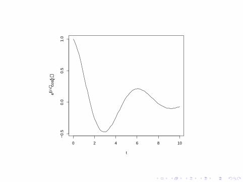
That leads to a solution of the form

y(t) = Aeλt cos(ω0t + φ)

where the quantities λ and ω0 are determined by the physicalcharacteristics of our system and the terms A and φ aredetermined by the initial conditions.

Typically λ < 0, and then the solution makes perfect sense, theoscillations die down eventually at a rate determined by λ, whichdepends on the mass m and the damping coefficient b.

0 2 4 6 8 10

−0.

50.

00.

51.

0

t

e((t4))

cos((

t))

Forced vibrations

So, up to this point the solution is pretty straight-forward. Butwhat about the case where we have a forcing frequency? What ifwe shake the block?

In this case our differential equation is then

y +b

my +

k

my = F

where F is some forcing input, let’s assume that F = F0 cos(ωt)

Again consider the simple model without damping

y +k

my = F0 cos(ωt), where

√k/m 6= ω

In this case the solution will look like this

y(t) = A cos(ω0t + φ) +F0

m(ω20 − ω2)

cos(ωt).

If φ = 0 then the solution is

y(t) =F0

m(ω20 − ω2)

cos(ωt − ω0t)

0 10 20 30 40 50 60

−1.

0−

0.5

0.0

0.5

1.0

t

f

Resonant forcing frequencies

What about the case where ω0 = ω?

In this case the solution then becomes

y(t) = cos(ω0t)F0

2mω0t sin(ω0t)

In reality there is always some form of damping or some limitationon the magnitude of y(t), but in practice this use of a resonantforcing frequency can be useful.

0 10 20 30 40 50 60

−15

−10

−5

05

1015

t

g

What does this have to do with the beam problem?

Well the beam does behave like a spring. The vibrations of thebeam are in fact pretty well modeled as a second order differentialequation.

The State-Space ModelIn order to get MATLAB to solve a second order differentialequation, it needs to be written as a set of two first orderdifferential equations. This is actually quite simple. Given ourequation

y +b

my +

k

my = 0.

Let

z1 = y(t)

z2 = y

then

z1 = z2

z2 = − k

mz1 −

b

mz2

In matrix form then this can be written as[z1

z2

]=

[0 1

−k/m −b/m

] [z1

z2

]with the initial conditions

z0 =

[y0

y0

]which is in a form that MATLAB can handle.

The Inverse Problem

What if we didn’t know m, b or k?

This is the inverse problem, given some observed data can we findout the values for those parameters?