Introduction to the Statistical

Software R

First Chapters, in Development

Werner Stahel, Seminar fur Statistik

ETH Zurich

September 2009

c© Reproduction for commercial use subject towritten consent by the Seminar fur Statistik

This document gives an introduction to the statistical programming language S,which forms the basis of the commercial package S-Plus and the free software R.Since the text only treats basic elements of the language, it covers both implemen-tations.

2

Contents

1 Introduction 1

1.1 What is R? . . . . . . . . . . . . . . . . . . . . . . . . . . . . . . . . . . . . 1

1.2 Other Statistical Software . . . . . . . . . . . . . . . . . . . . . . . . . . . . 1

1.3 Goals . . . . . . . . . . . . . . . . . . . . . . . . . . . . . . . . . . . . . . . 2

1.4 Introductory Example . . . . . . . . . . . . . . . . . . . . . . . . . . . . . . 2

1.5 Using R . . . . . . . . . . . . . . . . . . . . . . . . . . . . . . . . . . . . . . 4

1.6 Scripts and Editors . . . . . . . . . . . . . . . . . . . . . . . . . . . . . . . . 5

2 Basics 7

2.1 Vectors . . . . . . . . . . . . . . . . . . . . . . . . . . . . . . . . . . . . . . 7

2.2 Arithmetics . . . . . . . . . . . . . . . . . . . . . . . . . . . . . . . . . . . . 8

2.3 Character Vectors . . . . . . . . . . . . . . . . . . . . . . . . . . . . . . . . 9

2.4 Logical Vectors . . . . . . . . . . . . . . . . . . . . . . . . . . . . . . . . . . 9

2.5 Selecting Elements . . . . . . . . . . . . . . . . . . . . . . . . . . . . . . . . 10

2.6 Matrices . . . . . . . . . . . . . . . . . . . . . . . . . . . . . . . . . . . . . . 11

3 Simple Statistics 14

3.1 Simple Statistical Functions . . . . . . . . . . . . . . . . . . . . . . . . . . . 14

3.2 Hypothesis Tests . . . . . . . . . . . . . . . . . . . . . . . . . . . . . . . . . 15

3.3 Statistical Models, Formula Objects . . . . . . . . . . . . . . . . . . . . . . 16

4 Graphics 17

4.1 Overview . . . . . . . . . . . . . . . . . . . . . . . . . . . . . . . . . . . . . 17

4.2 Scatterplot . . . . . . . . . . . . . . . . . . . . . . . . . . . . . . . . . . . . 17

4.3 Boxplot . . . . . . . . . . . . . . . . . . . . . . . . . . . . . . . . . . . . . . 19

4.4 Adding Points and Lines to a Plot . . . . . . . . . . . . . . . . . . . . . . . 19

4.5 Adding Text to a Plot . . . . . . . . . . . . . . . . . . . . . . . . . . . . . . 20

4.6 Interacting with a Plot . . . . . . . . . . . . . . . . . . . . . . . . . . . . . . 21

1 Introduction

1.1 What is R?

• R is a software environment for statistical data analysis.

• R is based on commands to be typed. It implements a programming language, calledthe S language, which was developped for efficient statistical data analysis and forimplementing statistical methods with limited effort.

• There is an inofficial menu based interface called R-Commander, which containsa collection of basic statistical methods. It may be expanded by more advanced usersto include methods used in their environment. This interface generates commandsand submits them to the system. We will not use it here since our goal is to enablethe reader to do more flexible analyses.

• Menus have the drawback that it is difficult to store or remember which buttonshave to be pushed to get a certain result. Commands can be stored and therebybe used to document the analysis and allow for easy repetition with changed data,options, or other variations.

• R is free software, available from http://www.r-project.org and maintainedfor the operating systems Linux, Mac OS X, Windows. Therefore, every one manconsulting service ...

• ... and every student and researcher who has no guts to write applications for moneyto purchase and maintain the system. It has therefore become the language forexchanging new methods among researchers. It gives everybody access to thenewly developed tools.

1.2 Other Statistical Software

• S-Plus: This system is also based on the S language. There are differences, however,such that one could say that S-Plus and R are two dialects of this language. S-Plus iscommercial, which makes it more attractive for companies who want to buy support.It features a menu system, which is another advantage if it should be a standardsoftware for a wide range of users.

• SPSS: This system is well known and highly developed. It contains a large collectionof standard procedures, and several more advanced ones in the direction of socialsciences.

• SAS: This is the classical, large statistical package – also the most expensive ge-neral package. It has developped into management of data bases and other generalcomputer tasks. It handles large data sets, and is sometimes best for complicatedanalyses.

R-Kurs, c© Seminar fur Statistik

2 1 INTRODUCTION

• Systat: Analysis of Variance, easy-to-use graphics system.

• There are many more packages, e.g. several that are common in econometrics.

• Excel also contains statistical methods, but they are quite limited. We do not re-commend to start statistical analyses in Excel. It can profitably be used to get thedataset ready.

• Matlab is a system for mathematical calculations. The statistical methods are li-mited in both content and implementation quality. The “paradigm” is very similarto the S language, as it implements a kind of language that has similar structure asthe S language but is less flexible and misses useful concepts.

1.3 Goals

a These notes are meant to go with an introductory course for R. In an extended version,the course may comprise seven sessions of one lesson of lecture and one of exercises each. Itintroduces the basic concepts and most used general methods, including simple statisticalanalyses and graphical displays, and ends with an appetizer on linear regression.

b Some introductions into R or the S language go through the different concepts in a syste-matic way according to the structure of the language. These notes aim at starting fromthose notions that are needed in practice first to achieve useful results immediately. The-refore, we first introduce how a dataset is represented in R – even though this is in fact arather complicated structure – but postpone an exact description of the concept until later.Thus, common ways to use the system can be practiced from the start, and complicationsare discussed only when needed. If you prefer a more mathematical, systematic treatment,you should find other introductory texts on the web. Those documentations will also beuseful as systematic references once you have worked through this script.

c The participants and readers should be able to conduct statistical analyses as they willknow how to handle R and how to get the necessary information for finding and usingspecific methods. They should have the basic knowledge for exploiting the flexibility ofthe system by programming and writing their own functions.

1.4 Introductory Example

a Data, data.frame. Statistcal analyses start usually from a table or matrix of data. Arow of this table contains the values of all variables or characteristics of an observation.S stores such a data set in a so called data.frame. The variables may be numerical ofcategorical (or even complex numbers).

1.4. INTRODUCTORY EXAMPLE 3

b Importing data. The S function read.table is used to make a dataset available to thesystem. The command

> d.sport <− read.table(

"http://stat.ethz.ch/Teaching/Datasets/WBL/sport.dat",header=TRUE)

reads the data of the text file ”sport.dat” from the given web site and stores it under thename d.sport.

c Dataset d.sport If we now type

> d.sport

in the R command window, we get

weit kugel hoch disc stab speer punkte

OBRIEN 7.57 15.66 207 48.78 500 66.90 8824

BUSEMANN 8.07 13.60 204 45.04 480 66.86 8706

DVORAK 7.60 15.82 198 46.28 470 70.16 8664

: : : : : : : :

: : : : : : : :

: : : : : : : :

CHMARA 7.75 14.51 210 42.60 490 54.84 8249

d Selecting a variable.

> d.sport[,"kugel"]

extracts the variable ”kugel”. (Brackets are generally used to select parts of “objects”.)

e A histogram. Function hist draws a histogram in a graphics window:

> hist(d.sport[,"kugel"])

R opens such a window if none has been opened yet. (Alternatively, one would need orwant to call a function which does that, like wingraph() oder motif().)

f Scatter plots. One of the most basic graphical displays of data is certainly the scatterplot.

> plot(d.sport[,"kugel"], d.sport[,"speer"])

plots the values of speer (vertrically) against the values of kugel (horizontally).

Instead of using the link directly, you may store the file on your computer, e.g., in a directory

C:/Home/Datasets. Then, the command is d.sport <− read.table("C:/Home/Datasets/sport.dat",

header=TRUE).

4 1 INTRODUCTION

g Scatterplot matrix.

> pairs(d.sport)

generates a whole matrix of scatter plots, showing the plot of each variable of the datasetagainst every other one.

1.5 Using R

a Let us resume basic characteristics of using R.

• Within a window running R, you will see the prompt >. You type a command andget a result and a new prompt.

An incomplete statement can be continued on the next line> plot(d.sport[,"kugel"],

+ d.sport[,"speer"])

• R stores “objects” in your “workspace”:> d.sport <- read.table(...)

defines the object d.sport. More specifically, d.sport is a “data.frame”.

• Objects have names like a, fun, d.sport . Names start by a letter and arecontinued by letters or digits. The dot (.) and underscore ( ) are treated like letters.Blanks and special characters terminate the name. Upper and lower case letters aredistinct.

There are, of course, some reserved names, like if, for, break. The system will issuean error message if you try to use one of them to store your own stuff. Then, thereare some hazards: You can overwrite basic functions or constants (as by pi <- 5).

• R provides a huge number of functions and other objects. This is the treasure!There are many functions which are part of the “core system”, and even more whichare provided by advanced users in so-called “packages” – and remain under theirresponsibility. We will come back to this point later.

b An R statement consists of

• a name of an object only. This makes the system display the object.

• a call to a function or an arithmetic expression. This leads to a graphical or numericalresult (or sometimes to a “side effect” like changing an option).

• an assignment, consisting of a name, the arrow <-, and a call to a function orarithmetic expression> a <- 2*pi/360

> mn <- mean(d.sport[,"kugel"])

stores the mean of d.sport[,"kugel"] under the name mn.Note. The assignment can be denoted by =, but we do not recommend this since itmay lead to confusion.

1.6. SCRIPTS AND EDITORS 5

c Calling a function. Calls of functions are the core business of using the S language.

Functions have mandatory arguments, which the program needs to do something sen-sible, like the data it should work with. Additionally, there usually are optional argu-ments. If such an argument is not specified, the program has a default value – whichis thus changed by giving a value to the argument. For example, hist has an optionalargument nclass (and many more).

> hist(d.sport[,"kugel"], nclass=10)

generates a histogram with about 10 classes.

d Help. There is no need to learn which arguments all the functions have. Typing

> help(hist)

oder

> ?hist

one gets a window with a description of the goals and all the arguments of the functionhist. This information often comes with a lot of jargon, however, which you do not needto understand at this point.

It is often very useful to look at the examples that are given in the help documentation.They can be executed automatically by typing

> example(hist)

e Objects. As you continue working, you will store more and more objects in your“workspace”.You can get a list of their names by typing> objects()

If you want to remove one of them (a1 and data), you type> rm(a1, data)

You can delete many objects with a whole list of objects, see later.

f Ending the session. Type

> q()

to leave the system. R will ask: Save workspace image? If you answer y, then you willhave the objects that you generated at your disposal next time you enter R – and thiswill be useful for the exercises. Therefore, type y. When analyzing data, it may be lessdesirable to do that, see later.

1.6 Scripts and Editors

a Instead of typing commands into the R window, you can generate commands by an editorand then “send” them to the R window – and later modify (correct) them and send again.

6 1 INTRODUCTION

b Text Editors supporting R. The following editors support the use of R by supplying”buttons” to send the current line or the marked region of text to the R window.

• WinEdt: http://www.winedt.com/

• Emacs: http://www.gnu.org/software/emacs/, enhanced byESS: http://stat.ethz.ch/ESS/

• Tinn-R: http://www.sciviews.org/Tinn-R/ . This editor is used in the exercisesdone in class.

• For Mac: ...

c The Tinn-R Window

2 Basics

2.1 Vectorsa Creating vectors. A vector is a collection of numbers into one object. Above, we have

used d.sport[,"kugel"] Here we store it as the vector t.v.

> t.v <− d.sport[,"kugel"]

> t.v

[1] 15.66 13.60 15.82 15.31 16.32 14.01 13.53 14.71 16.91 15.57 14.85

[12] 15.52 16.97 14.69 14.51

shows the values of variable kugel for all observations (athletes). The number in bracketsat the beginning of the lines indicate which element of the vector appears first on the line– 15.52 is the 12th observation.

b A vector can also be generated by directly typing a bunch of numbers, using the S functionc (concatenate):

> t.a <− c(3.1, 5, -0.7, 0.9, 1.7)

(Function c behaves somewhat atypical: There may be an arbitrary number of arguments– they are all concatenated to form the result.)

c Function seq generates seqences of numbers with constant difference,

> seq(0,3,by=0.5)

[1] 0.0 0.5 1.0 1.5 2.0 2.5 3.0

For the most used sequences of this kind, consecutive integers, S reserves the colon:

> 1:9

[1] 1 2 3 4 5 6 7 8 9

is equivalent to seq(1,9,by=1) or seq(1,9).

d Function rep generates vectors by repeting numbers. The simplest version is

> rep(0.7,5)

[1] 0.7 0.7 0.7 0.7 0.7

It also does more complicated jobs,

> rep(c(1,3,5),length=8)

[1] 1 3 5 1 3 5 1 3

e Now we want to do something useful with vectors. Table 2.1.e lists some simple functionswhich are applicable for vectors.

R-Kurs, c© Seminar fur Statistik

8 2 BASICS

call, example explanation

length(t.v) number of elementsrev(t.v) reverse the order of the elementssort(t.v) elements sorted (by increasing order)rank ranksunique all different elementssum(t.v) sum of all elementscumsum(t.v) cumulative sumsmean(t.v) arithmetic meanvar(t.v) empirical variancerange(t.v) range

Tabelle 2.1.e: Functions for numerical vectors

2.2 Arithmetics

a Of course, R can calculate!

> 2+5

[1] 7

The basic arithmetic operations are denoted by + , - , * , / . The hat character ^

stands for exponentiation.

b For vectors, the operations are done elementwise,

> (2:5) ^ c(2,3,1,0)

[1] 4 27 4 1

The priorities are as usual. Parantheses are useful in case of doubt.

c One of the operands may be a single number,

> (2:5) ^ 2

[1] 4 9 16 25

If both are vectors, but of different lengths, the shorter is recycled until the longer lengthis reached,

> (1:5)-(0:1)

[1] 1 1 3 3 5

Since there remains a rest in this example, S gives a warning,

Warning message:

longer object length is not a multiple of shorter object length in:

(1:5) - (0:1)

(This may often be useful – on the other hand, if the larger length happens to be a multipleof the shorter one, you do not get any message!)

See also help("Arithmetic").

2.3. CHARACTER VECTORS 9

2.3 Character Vectors

a Alphanumerical vectors. Like all programming languages, S can deal with “words” orcharacter strings. A vector of such strings results from

> t.b <− c("Andi" "Bettina", "Christian")

b A very useful function to create strings is paste, which converts the given values tocharacter strings if needed, and then pastes them together,

> paste("ABC","XYZ",17)

[1] "ABC XYZ 17"

The item used to separate the original string is given by the argument sep (with a blankas default value),

> paste("ABC","IJK","XYZ",sep=":")

[1] "ABC:IJK:XYZ"

No separation is obtained by setting sep="".

c If the arguments are vectors, the result is a vector, too,

> paste(c("a","b","c"),1:3)

[1] "a 1" "b 2" "c 3"

If the elements of a vector should be pasted together, the argument collapse must bespecified:

> paste(letters, collapse="; ")

[1] "a; b; c; d; e; f; g; h; i; j; k; l; m; n; o; p; q; r; s; t; u; v; w;

x; y; z"

pastes the alphabeth, which is available from the system as letters.

d Function paste is thus very flexible. As with c, the number of arguments is arbitrary.Therefore, the special arguments sep and collapse – of which only one can be used –need to be called by their name.

2.4 Logical Vectors

a Besides numerical and character vectors there is the logical type, which only containsvalues TRUE or FALSE. They will prove useful in the next paragraph. They usually appearas the result of comparisons,

> (1:5)>=3

[1] FALSE FALSE TRUE TRUE TRUE

For the first and second element of (1:5), the inequality is not fulfilled (FALSE), for theremaining three, it is valid (TRUE).

10 2 BASICS

b The comparison operators are written as

<, <=, >, >=, ==, !=.

Note that equality is denoted by two equal signs, since the single = is used to determinethe values of arguments in a function – and it can be used to replace the assignmentsymbol <-.

See also help("Comparison").

c The logical operators are denoted by & (and), | (or), ! (not).

> t.i <− (t.v>2)&(t.v<5)

yields TRUE for in the places of those elements of t.v, the values of which are between 2and 5.

2.5 Selecting Elements

a Often, we want to restrict an analysis to a part of the entire dataset. We have seen howto select a column of a data.frame (1.4.d) using the brackets [ ]. These are also useful toextract parts of vectors.

b There are 3 possibilities to do so:

• Indices (integers):

> t.v[c(1,3,5)]

[1] 15.66 15.82 16.32

> d.sport[c(1,3,5),1:3]

weit kugel hoch

OBRIEN 7.57 15.66 207

DVORAK 7.60 15.82 198

HAMALAINEN 7.48 16.32 198

To drop elements, use negative indices:> d.sport[-(3:12),c("kugel","punkte")]

kugel punkte

OBRIEN 15.66 8824

BUSEMANN 13.60 8706

CHMARA 14.51 8249

• Logical vectors:

> t.a[c(TRUE,FALSE,TRUE,TRUE,FALSE,FALSE)]

[1] 3.1 -0.7 0.9

> d.sport[t.v > 16,c(2,7)]

kugel punkte

HAMALAINEN 16.32 8613

PENALVER 16.91 8307

SMITH 16.97 8271

2.6. MATRICES 11

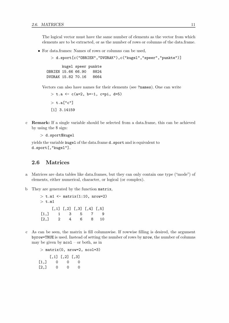
The logical vector must have the same number of elements as the vector from whichelements are to be extracted, or as the number of rows or columns of the data.frame.

• For data.frames: Names of rows or columns can be used,

> d.sport[c("OBRIEN","DVORAK"),c("kugel","speer","punkte")]

kugel speer punkte

OBRIEN 15.66 66.90 8824

DVORAK 15.82 70.16 8664

Vectors can also have names for their elements (see ?names). One can write

> t.a <- c(a=2, b=-1, c=pi, d=5)

> t.a["c"]

[1] 3.14159

c Remark: If a single variable should be selected from a data.frame, this can be achievedby using the $ sign:

> d.sport$kugel

yields the variable kugel of the data.frame d.sport and is equivalent tod.sport[,"kugel"].

2.6 Matrices

a Matrices are data tables like data.frames, but they can only contain one type (“mode”) ofelements, either numerical, character, or logical (or complex).

b They are generated by the function matrix,

> t.m1 <- matrix(1:10, nrow=2)

> t.m1

[,1] [,2] [,3] [,4] [,5]

[1,] 1 3 5 7 9

[2,] 2 4 6 8 10

c As can be seen, the matrix is fill columnwise. If rowwise filling is desired, the argumentbyrow=TRUE is used. Instead of setting the number of rows by nrow, the number of columnsmay be given by ncol – or both, as in

> matrix(0, nrow=2, ncol=3)

[,1] [,2] [,3]

[1,] 0 0 0

[2,] 0 0 0

12 2 BASICS

d A data.frame can be converted into a matrix by as.matrix,

> t.sportmat <− as.matrix(d.sport)

If a variable is categorical (a“factor”), as.matrix converts all columns into type character.The function data.matrix codes factors by integers and always yields a numerical matrix.

e Matrices can also be obtained by pasting vectors together, either as rows (rbind) or ascolumns (cbind),

> cbind(4:6,13:15)

[,1] [,2]

[1,] 4 13

[2,] 5 14

[3,] 6 15

f The functions nrow(t.m), ncol(t.m), dim(t.m) return the number of rows, of columns,and both, respectively.

> dim(t.m)

[1] 2 5

g Extraction of elements as with data.frames:

> t.m1[2,1:3]

[1] 2 4 6

Selection by names of rows and columns is also possible if such names have been stored.See ?dimnames.

h Arrays. Arrays of more than 2 dimensions can be generated by function array. Sincethey are rarely used, we do not address this issue.

i Multiplication of matrices. The S language is based on thinking in terms of vec-tors and matrices instead of single numbers. The basic operation for matrices is matrixmultiplication. It is requested by the symbols %*%,

> t.m1 %*% t(t.m2)

[,1] [,2]

[1,] 95 220

[2,] 110 260

j One of the operands may be a vector. It is then treated as a one row or one column matrixif this leads to a possible matrix multiplication.

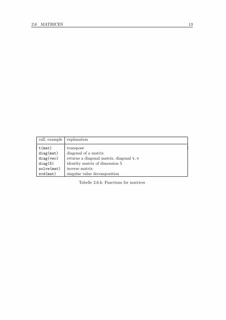
k Functions for matrices. S includes all important functions of linear algebra, see Table2.6.k for a selection.

2.6. MATRICES 13

call, example explanation

t(mat) transposediag(mat) diagonal of a matrixdiag(vec) returns a diagonal matrix, diagonal t.vdiag(5) identity matrix of dimension 5solve(mat) inverse matrixsvd(mat) singular value decomposition

Tabelle 2.6.k: Functions for matrices

3 Simple Statistics

3.1 Simple Statistical Functions

a This section presents some functions of S which implement methods for simple statisticalproblems like one- and two-sample tests.

b Tables. Function table counts the numbers of times each value appears,

> table(d.blast[,"loc"])

L1 L2 L3 L4 L5 L6

14 10 14 10 24 24

Location L1 thus occured 14 times in the dataset.

c It continuous data should first be classified, function cut proves useful,

> t.speer <− cut(d.sport[,"speer"],seq(50,75,5))

> table(t.speer)

(50,55] (55,60] (60,65] (65,70] (70,75]

3 2 3 6 1

A similar result is obtained by function hist with argument plot=FALSE,

> hist(d.sport[,"speer"], plot=FALSE)

(The class limits happen to be those chosen before in this example.)

d Function table also generates cross-classification tables,

> t.kugel <− cut(d.sport[,"kugel"],seq(13,17,1))

> table(t.kugel, t.speer)

t.speer

t.kugel (50,55] (55,60] (60,65] (65,70] (70,75]

(13,14] 0 0 0 2 0

(14,15] 3 0 0 2 0

(15,16] 0 0 2 2 1

(16,17] 0 2 1 0 0

– a pity that no marginal sums or percentages are given!

R-Kurs, c© Seminar fur Statistik

3.2. HYPOTHESIS TESTS 15

e Numerical Descriptive Statistics.

Estimation of a “location parameter”:

> mean(x); median(x)

Variance: var(x)

correlation:

> cor(d.sport[,"kugel"], d.sport[,"speer"])

[1] -0.146

Correlation matrix:

> t.cor <- cor(d.sport[,1:3])

> round(100*t.cor)

weit kugel hoch

weit 100 -63 34

kugel -63 100 -9

hoch 34 -9 100

3.2 Hypothesis Tests

a Tests and Confidence Intervals. For Tests and Confidence Intervals for the parameterof a binomial distribution (that is, for a probability of an event), there is the functionbinom.test:

> binom.test(3,20, p=0.4)

yields a rather extensive result including a p value for the test of the null hypothesisπ = 0.4 and a confidence interval.

b For two independent samples, functions wilcox.test and t.test compute results ofa Wilcoxon-Mann-Whitney rank sum test and a t test, respectively,

> t.hh <− d.sport[,"hoch"]>200

> t.kugel <− d.sport[,"kugel"]

> wilcox.test(t.kugel[t.hh],t.kugel[!t.hh])

Wilcoxon rank sum test

data: t.kugel[t.hh] and t.kugel[!t.hh]

W = 20, p-value = 0.4559

alternative hypothesis: true mu is not equal to 0

> t.test(t.kugel[t.hh],t.kugel[!t.hh], var.equal = TRUE)

Two Sample t-test

data: t.kugel[t.hh] and t.kugel[!t.hh]

t = -0.8066, df = 13, p-value = 0.4344

alternative hypothesis: true difference in means is not equal to 0

95 percent confidence interval:

16 3 SIMPLE STATISTICS

-1.694 0.773

sample estimates:

mean of x mean of y

15.01 15.47

For paired samples or a single sample, the same functions are applied, setting the argumentpaired=TRUE.

3.3 Statistical Models, Formula Objects

a An important part of statistics is concerned with exploring relationships between variables.In statistical Regression and Analysis of Variance, models for such analyses are construc-ted. A specific “language” or syntax has been introduced to formalize such models. It isused in other statistical packages, too.

This formula syntax can also be used to specify graphical displays efficiently. We thereforeintroduce them here in their simplest form, even though regression models will be treatedonly later.

b A simple formula looks as follows:

kugel ∼ speer + weit

Each formula contains the symbol ‘∼’ (Tilde). To the left of it appears the“target variable”(kugel), to the right, the “input variables” (speer, weit) of the model. In a scatterplot,the target variable is used on the vertical axis, whereas the input variables appear on thehorizontal axis. The variables on the right hand side are separated by ‘+’ – even thoughno summation is done.

More on formulas will be said in the chapter on Regression.

c A formula can be stored in the usual way. It remains a formula, that is, a kind of phrasein the formula language. Only when it is handed over to a function that knows what todo with it, variables are evaluated to become concrete numerical values again.

d An example of such a function is plot:

> plot(kugel ∼ speer, data=d.sport)

generates the scatterplot of the variables kugel against speer of the dataset d.sport. Wewill discuss variations of such plots in the following chapter.

Note that the symbols used in the formula are interpreted as columns of the data.framegiven by the argument data (if that argument is specified). This is typical for the use offormulas in the functions that accept formulas as arguments.

e Note. We have used the function plot before. Then, the first argument defined the hori-zontal coordinates and was a vector. Here, the first argument is a formula. This reflects animportant concept of the S language: Some functions behave quite differently dependingon the nature of the first argument. They are called “generic functions” and make the Slanguage an “object oriented” programming language. More about this concept follows inChapter 4.

4 Graphics

4.1 Overview

a Several R graphics functions have been presented so far:> plot(d.sport[,"kugel"], d.sport[,"speer"],

+ xlab="ball push", ylab="javelin", pch=7)

> plot(punkte ∼ kugel+speer, data=d.sport)

> pairs(d.sport)

> boxplot(sleep[1:10,"extra"],sleep[11:20,"extra"],ylab="extra")

Many more functions are available and will be introduced:scatter.smooth(), matplot(), image(), ...lines(), points(), . . .par(), identify(), dev.new(), . . .

b There are 6 kinds of R graphics functions:

• High-level plotting functions such as plot()⇒ generate a new graphical display of data.

• Low-level plotting functions such as lines()⇒ add further graphical elements to an existing graph.

• “Interactive” functions such as identify()⇒ enhance or collect information interactively from a graph.

• “Control” functions such as par()⇒ control the appearance of graphs.

• “Device” control functions such as dev.new()⇒ to manipulate windows and files that display or store graphs.

4.2 Scatterplot

a The most common graphical display shows the values of two variables, plotted againsteach other. The (first) syntax is

> plot(x=x, y=y, main="...", xlab="...",

ylab="...", ...)

x,y are two numeric vectors.Example:> plot(x=meuse[,"x"], y=meuse[,"y"], xlab="easting", ylab="northing",

+ main="sampling locations")

R-Kurs, c© Seminar fur Statistik

18 4 GRAPHICS

b Three alternative ways to invoke plot():

• Plot of the values of a single vector against the position indices of the vector elements:> plot(meuse[,"zinc"], ylab = "zinc")

• Scatterplot of two columns of a matrix or a dataframe> plot(meuse[,c("x","y")])

• Use of a model “formula” to select y and x variable from a data frame:> plot(zinc∼dist, data=meuse)

Note: y∼x: The variable to be used on the vertical axis comes first.

c Many arguments of plot() are common to many graphics functions:

• main="...", xlab="...", ylab="...", where...: any character string⇒ used to set title and labels of axes

• log="x", log="y", log="xy"⇒ for logarithmic scaling of axes

• xlim=c(xmin,xmax), ylim=c(ymin,ymax)

⇒ set ranges for the values to be displayed.

• asp=n

⇒ set “aspect ratio” of axes, i.e. ratio of lengths of “measurement” units on y andx axis. This is most often used to ensure that the scales of both axis are equal whendisplaying a geographical location or two geometrical measurements of an object, bysetting asp = 1.

• pch=i or pch="c"⇒ select the plotting symbol(s)

c: a (vector of) single character(s) ori: a (vector of) integer(s) to select one of the built-in geometrical symbols (square,cricle, triangle, cross, ..., see ?points for a list).If a vector is given, different symbols will be used for the different points (recycledif necessary).

• cex=n

⇒ choose the size of the symbols, relative to the standard size that the plot

function would choose by default. A vector can be given as with pch.

• col=i or col="color"⇒ choose the size and color of symbols

color : name of color in english (col = "red"). A vector can again be given as withpch.

4.3. BOXPLOT 19

4.3 Boxplot

a Boxplots show the most important aspects of (the distribution of) a sample in a simpleway. Syntax:

> boxplot(x=x, notch=l, horizontal=l, ...)

notch = TRUE: “notches” are added to roughly test whether two medians are significantlydifferenthorizontal = TRUE: boxplots are shown horizontally. (There is no argument vertical.)

Example:> boxplot(x=meuse[,"zinc"], notch=TRUE, horizontal=TRUE, log="x",

+ xlab="zinc content")

b Variations of boxplots:

• Boxplot of several variables in same graph:> boxplot(meuse[,c("zinc","lead")], horizontal=TRUE, log="x")

• Boxplots of several groups for one variable:> boxplot(zinc∼ffreq, data=meuse)

4.4 Adding Points and Lines to a Plot

a Use points() to add further points to a graph created before by a high-level graphicsfunction.> points(x=x, y=y, pch=i, col= , cex=n, ...)

Example:> plot(lead∼dist.m, data=meuse, ylim=c(10,1000), log="y")

> points(meuse[,c("dist.m","copper")],

+ col="red", pch=3)

b Lines can be added by lines() to a graph.> lines(x=x, y=y, col= , lty= , lwd=n,...)

lty=i or lty="linetype" (keyword): type of linen: line width relative to default value

Example:> plot(y∼x, meuse, asp=1)

> lines(meuse.riv, lty="dotted", lwd=2.5, col= "cyan")

c Straight lines through the whole plotting area can be added by abline() to a graph.> abline(a=n, b=n, h=v, v=v, ...)

Provide either values to a (intercept) and b (slope) or h=v as the (y) position(s) of hori-zontal or v=v as the (x) position(s) of vertical straight line(s).

Example:> plot(lead∼dist.m, meuse, asp=1)

> abline(h=c(200,500), lty="dotted", col=c("orange","red"))

> abline(a=300, b=-1, lty="3313", lwd=3)

20 4 GRAPHICS

d Line segments are added by segments().> segments(x0=v, y0=v, x1=v, x2=v, ...)

Line segments are drawn from the points (x0, y0) to the points (x1, y1) (v numericvectors of same length).

Example:> plot(y∼x, meuse)

> t.xr <- range(meuse[,"x"])

> t.yr <- range(meuse[,"y"])

> segments(x0=rep(t.xr[1],2), y0=t.yr, x1=rep(t.xr[2],2), y1=t.yr[2:1] )

e Polygons are added by polygon().> polygon(x=x, y=y, density=n, angle=n, border= , col= ,...)

Provide values to density and angle for hachuring and to border and col for borderand fill color of polygons. ???

Example:> plot(y∼x, meuse, asp=1)

> polygon(meuse.riv, border="blue", col="cyan", angle=135, density=10)

4.5 Adding Text to a Plot

a Points in a scatterplot are labelled by text().> text(x=x, y=y, labels= , pos=i, ...)

Provide a vector of character strings to labels. The argument pos controls whether thetext is plotted below (1), to the left (2), above (3) or to the right (4) of the points.

Example:> plot(y∼x, meuse, asp=1, type="n")

> text(meuse[,c("x","y")], cex=0.7, labels=meuse[,"landuse"])

b Legend. Place a legend explaining any different symbols or line types used by legend().> legend(x= , y=n, xjust=n, yjust=n,

legend= , col= , lty= , pch= ,...)

The position of the legend is either specified by x and y in combination with the argumentsxjust, yjust or by a keyword such as "bottomleft" as the first argument (cf.?legendfor details). legend contains the explanatory text as a vector of character strings. Oneor more of the remaining arguments will be specified by a vector of the same length aslegend and will give the symbols and line types (pch and lty), the symbol sizes (cex), orthe colors (col).

Example:> plot(meuse[,c("x","y")], asp=1, col=as.numeric(meuse[,"ffreq"]),

+ cex=sqrt(meuse[,"zinc"])/10)

> legend(x="topleft", pch=c(NA,rep(1,3)),

+ col=c("black","black","red","green"),

+ legend=c("flooding", "often", "intermediate", "rarely"))

4.6. INTERACTING WITH A PLOT 21

4.6 Interacting with a Plot

a Points in plots are identified and querried interactively by identify().> identify(x=x, y=y, labels= )

Provide a character or numeric vector of the same length as x and y to labels for labellingidentified points accordingly. Click the right hand mouse button to stop identifying.

Example:> plot(meuse[,c("x","y")], asp=1, cex=sqrt(meuse[,"zinc"])/10))

> t.i <- identify(meuse[,c("x","y")], labels=meuse[,"zinc"])

Now, the sequence numbers of the identified points are available as t.i for further use.

b Read the coordinates of interactively selected points from plots by using locator().> locator(n=i, type="p")

You can either specify the number i of points to locate in advance or right-click to stoplocating points.Example:> plot(meuse[,c("x","y")], asp=1)

> polygon(locator())