introduction to the theory of computation - …david/courses/csc236_w14/resources/... · contents...
TRANSCRIPT
David Liu
Introduction to the Theory ofComputation
Lecture Notes and Exercises for CSC236
Department of Computer ScienceUniversity of Toronto


Contents
Introduction 5
Induction 9
Recursion 27
Program Correctness 45
Regular Languages & Finite Automata 63
In Which We Say Goodbye 79

Introduction
There is a common misconception held by our students, the students ofother disciplines, and the public at large about the nature of computerscience. So before we begin our study this semester, let us clear upexactly what we will be learning: computer science is not the study ofprogramming, any more than chemistry is the study of test tubes ormath the study of calculators. To be sure, programming ability is avital tool in any computer scientist’s repertoire, but it is still a tool inservice to a higher goal.
Computer science is the study of problem-solving. Unlike other dis-ciplines, where researchers use their skill, experience, and luck to solveproblems at the frontier of human knowledge, computer science asks:What is problem-solving? How are problems solved? Why are someproblems easier to solve than others? How can we measure the qualityof a problem’s solution?
Even the many who go into industryconfront these questions on a dailybasis in their work!
It should come as no surprise that the field of computer sciencepredates the invention of computers, since humans have been solvingproblems for millennia. Our English word algorithm, a sequence ofsteps taken to solve a problem, is named after the Persian mathemati-cian Muhammad ibn Musa al-Khwarizmi, whose mathematics textswere compendia of mathematics computational procedures. In 1936,
The word algebra is derived from theword al-jabr, appearing in the titleof one of his books, describing theoperation of subtracting a number fromboth sides of an equation.
Alan Turing, one of the fathers of modern computer science, devel-oped the Turing Machine, a theoretical model of computation which iswidely believed to be just as powerful as all programming languagesin existence today. In one of the earliest and most fundamental results
A little earlier, Alonzo Church (whowould later supervise Turing) devel-oped the lambda calculus, an alternativemodel of computation that forms thephilosophical basis for functional pro-gramming languages like Haskell andML.
in computer science, Turing proved that there are some problems thatcannot be solved by any computer that has ever or will ever be built,before computers had been invented at all!
But Why Do I Care?
A programmer’s value lies not in her ability to write code, but to un-derstand problems and design solutions – a much harder task. Be-

6 david liu
ginning programmers often write code by trial and error (“Does thiscompile? What if I add this line?”), which indicates not a lack ofprogramming experience, but a lack of design experience. On beingpresented with a problem, many students often jump straight to thecomputer – even if they have no idea what they are going to write!And even when the code is complete, they are at a loss when askedthe two fundamental questions: Why is your code correct, and is it a
“My code is correct because it passedall of the tests” is passable but unsat-isfying. What I really want to know ishow your code works.good solution?
In this course, you will learn the skills necessary to answer both ofthese questions, improving both your ability to reason about the codeyou write, and your ability to communicate your thinking with others.These skills will help you design cleaner and more efficient programs,and clearly document and present your code. Of course, like all skills,you will practice and refine these throughout your university educa-tion and in your careers; in fact, you have started formally reasoningabout your code in CSC165 already.
Overview of this Course
The first section of the course introduces the powerful proof techniqueof induction. We will see how inductive arguments can be used in Philosophy has another meaning of
“inductive reasoning” which we do notuse here. The arguments generally usedin mathematics, including mathemat-ical induction, are forms of deductivereasoning.
many different mathematical settings; you will master the structureand style of inductive proofs, so that later in the course you will noteven blink when asked to read or write a “proof by induction.”
From induction, we turn our attention to the runtime analysis ofrecursive programs. You have done this already for non-recursive pro-grams, but did not have the tools necessary for recursive ones. Wewill see that (mathematical) induction and (programming) recursionare two sides of the same coin, and with induction analysing recursiveprograms becomes easy as cake. After these lessons, you will always Some might even say, chocolate cake.
be able to evaluate your recursive code based on its runtime, a verysignificant development factor!
We next turn our attention to the correctness of both recursive andnon-recursive programs. You already have some intuition about whyyour programs are correct; we will teach you how to formalize thisintuition into mathematically rigorous arguments, so that you mayreason about the code you write and determine errors without the useof testing.
This is not to say tests are unnecessary.The methods we’ll teach you in thiscourse are quite tricky for larger soft-ware systems. However, a more matureunderstanding of your own code cer-tainly facilitates finding and debuggingerrors.
Finally, we will turn our attention to the simplest model of compu-tation, finite automata. This serves as both an introduction to morecomplex computational models like Turing Machines, and also formallanguage theory through the intimate connection between finite au-tomata and regular languages. Regular languages and automata havemany other applications in computer science, from text-based pattern
introduction to the theory of computation 7
matching to modelling biological processes.
Prerequisite Knowledge
CSC236 is mainly a theoretical course, the successor to CSC165. Thisis fundamentally a computer science course, though, so while math-ematics will play an important role in our thinking, we will mainlydraw motivation from computer science concepts. Also, you will beexpected to both read and write Python code at the level of CSC148.Here are some brief reminders about things you need to know – andif you find that don’t remember something, review early!
Concepts from CSC165
In CSC165 you learned how to write proofs. This is the main objectof interest in CSC236, so you should be comfortable with this style ofwriting. However, one key difference is that we will not expect (noraward marks for) a particular proof structure – indentation is no longerrequired, and your proofs can be mixtures of mathematics, Englishparagraphs, pseudocode, and diagrams! Of course, we will still greatlyvalue clear, well-justified arguments, especially since the content willbe more complex. You should also be comfortable with the symbolic
So a technically correct solution that isextremely difficult to understand willnot receive full marks. Conversely, anincomplete solution which explainsclearly partial results (and possiblyeven what is left to do to completethe solution) will be marked moregenerously.
notation of the course; even though you are able to write your proofsin English now, writing questions using the formal notation is often agreat way of organizing your ideas and proofs.
You will also have to remember the fundamentals of Big-O algo-rithm analysis. You will be expected to read and analyse code in thesame style as CSC165, and it will be essential that you easily determinetight asymptotic bounds for common functions.
Concepts from CSC148
Recursion, recursion, recursion. If you liked using recursion CSC148,you’re in luck: induction, the central proof structure in this course, isthe abstract thinking behind designing recursive functions. And if youdidn’t like recursion or found it confusing, don’t worry! This coursewill give you a great opportunity to develop a better feel for recur-sive functions in general, and even give you a couple of programmingopportunities to get practical experience.
This is not to say you should forget everything you have done withiterative programs; loops will be present in our code throughout thiscourse, and will be the central object of study for a week or two whenwe discuss program correctness. In particular, you should be verycomfortable with the central design pattern of first-year python: com-
A design pattern is a common codingtemplate which can be used to solve avariety of different problems. “Loopingthrough a list” is arguably the simplestone.
8 david liu
puting on a list by processing its elements one at a time using a for orwhile loop.
You should also be comfortable with terminology associated withtrees which will come up occasionally throughout the course when wediscuss induction proofs. The last section of the course deals withregular languages; you should be familiar with the terminology asso-ciated with strings, including length, reversal, concatenation, and theempty string.
Induction
What is the sum of the numbers from 0 to n? This is a well-knownidentity you’ve probably seen before:
n
∑i=0
i =n(n + 1)
2.
A "proof" of this is attributed to Gauss: Although this is with high probabilityapocryphal.
1 + 2 + 3 + · · ·+ n− 1 + n = (1 + n) + (2 + n− 1) + (3 + n− 2) + · · ·= (n + 1) + (n + 1) + (n + 1) + · · ·
=n2(n + 1) (since there are
n2
pairs)
This isn’t exactly a formal proof – what if n is odd? – and although it We ignore the 0 in the summation, sincethis doesn’t change the sum.could be made into one, this proof is based on a mathematical “trick”
that doesn’t work for, say,n
∑i=0
i2. And while mathematical tricks are of-
ten useful, they’re hard to come up with! Induction gives us a differentway to tackle this problem that is astonishingly straightforward.
Recall the definition of a predicate from CSC165, a parametrized log-ical statement. Another way to view predicates is as a function thattakes in one or more arguments, and outputs either True or False.Some examples of predicates are:
EV(n) : n is even
GR(x, y) : x > y
FROSH(a) : a is a first-year university student
Every predicate has a domain, the set of its possible input values. Forexample, the above predicates could have domains N, R, and “the set We will always use the convention that
0 ∈N unless otherwise specified.of all UofT students,” respectively. Predicates gives us a precise wayof formulating English problems; the predicate that is relevant to ourexample is
P(n) :n
∑i=0
i =n(n + 1)
2.
You might be thinking right now: “Okay, now we’re going to prove
A common mistake: defining thepredicate to be something like
P(n) :n(n + 1)
2. Such an expres-
sion is wrong and misleading becauseit isn’t a True/False value, and so failsto capture precisely what we want toprove.

10 david liu
that P(n) is true.” But this is wrong, because we haven’t yet definedn! So in fact we want to prove that P(n) is true for all natural numbersn, or written symbolically, ∀n ∈ N, P(n). Here is how a formal proofmight go if we were in CSC165:
Proof of ∀n ∈N,n
∑i=0
i =n(n + 1)
2
Let n ∈N.# Want to prove that P(n) is true.
Case 1: Assume n is even.# Gauss’ trick...Then P(n) is true.
Case 2: Assume n is odd.# Gauss’ trick, with a twist?...Then P(n) is true.
Then in all cases, P(n) is true.Then ∀n ∈N, P(n). �
Instead, we’re going to see how induction gives us a different, easierway of proving the same thing.
The Induction Idea
Suppose we want to create a want to create a viral Youtube videofeaturing “The World’s Longest Domino Chain!!! (share plz)".
Of course, a static image like the one featured on the right is nogood for video; instead, once we have set it up we plan on recordingall of the dominoes falling in one continuous, epic take. It took a lotof effort to set up the chain, so we would like to make sure that it willwork; that is, that once we tip over the first domino, all the rest willfall. Of course, with dominoes the idea is rather straightforward, sincewe have arranged the dominoes precisely enough that any one fallingwill trigger the next one to fall. We can express this thinking a bit moreformally:
(1) The first domino will fall (when we push it).
(2) For each domino, if it falls, then the next one in the chain will fall(because each domino is close enough to its neighbours).
From these two ideas, we can conclude that
(3) Every domino in the chain will fall.

introduction to the theory of computation 11
We can apply the same reasoning to the set of natural numbers. In-stead of “every domino in the chain will fall,” suppose we want toprove that “for all n ∈ N, P(n) is true” where P(n) is some predi-cate. The analogues of the above statements in the context of naturalnumbers are
(1) P(0) is true (0 is the “first” natural number) The “is true” is redundant, but we willoften include these words for clarity.(2) ∀k ∈N, P(k)⇒ P(k + 1)
(3) ∀n ∈N, P(n) (is true)
Putting these together yields the Principle of Simple Induction (also simple/mathematical induction
known as Mathematical Induction):(P(0) ∧ ∀k ∈N, P(k)⇒ P(k + 1)
)⇒ ∀n ∈N, P(n)
A different, slightly more mathematical intuition for what inductionsays is that “P(0) is true, and P(1) is true because P(0) is true, and P(2)is true because P(1) is true, and P(3) is true because. . . ” However, itturns out that a more rigorous proof of simple induction doesn’t ex-ist from the basic arithmetic properties of the natural numbers alone.Therefore mathematicians accept the principle of induction as an ax-iom, a statement as fundamentally true as 1 + 1 = 2.
It certainly makes sense intuitively, andturns out to be equivalent to anotherfundamental math fact called the Well-Ordering Principle.This gives us a new way of proving a statement is true for all natural
numbers: instead of proving P(n) for an arbitrary n, just prove P(0),and then prove the link P(k) ⇒ P(k + 1) for arbitrary k. The formerstep is called the base case, while the latter is called the induction step.We’ll see exactly how such a proof goes by illustrating it with theopening example.
Example. Prove that for every natural number n,n
∑i=0
i =n(n + 1)
2.
The first few induction examplesin this chapter have a great deal ofstructure; this is only to help you learnthe necessary ingredients of inductionproofs. Unlike CSC165, we will notbe marking for a particular structurein this course, but you will probablyfind it helpful to use our keywords toorganize your proofs.
Proof. First, we define the predicate associated with this question. Thislets us determine exactly what it is we’re going to use in the inductionproof.
Step 1 (Define the Predicate) P(n) :n
∑i=0
i =n(n + 1)
2
It’s easy to miss this step, but without it, often you’ll have troubledeciding precisely what to write in your proofs.
Step 2 (Base Case): in this case, n = 0. We would like to prove thatP(0) is true. Recall the meaning of P:
P(0) :0
∑i=0
i =0(0 + 1)
2.
This statement is trivially true, because both sides of the equation areequal to 0.
For induction proofs, the base caseusually a very straightforward proof.In fact, if you find yourself stuck on thebase case, then it is likely that you’vemisunderstood the question and/or aretrying to prove the wrong predicate.
12 david liu
Step 3 (Induction Step): the goal is to prove that ∀k ∈ N, P(k) ⇒P(k+ 1). We adopt the proof structure from CSC165: let k ∈N be somearbitrary natural number, and assume P(k) is true. This antecedentassumption has a special name: the Induction Hypothesis. Explicitly,we assume that
k
∑i=0
i =k(k + 1)
2.
Now, we want to prove that P(k+ 1) is true, i.e., thatk+1
∑i=0
i =(k + 1)(k + 2)
2.
This can be done with a simple calculation:
We break up the sum by removing thelast element.
k+1
∑i=0
i =
(k
∑i=0
i
)+ (k + 1)
=k(k + 1)
2+ (k + 1) (By Induction Hypothesis)
= (k + 1)(
k2+ 1)
=(k + 1)(k + 2)
2
Therefore P(k + 1) holds. This completes the proof of the induction
The one structural requirement we dohave for this course is that you mustalways state exactly where you usethe induction hypothesis. We expectto see the words “by the inductionhypothesis” at least once in each ofyour proofs.
step: ∀k ∈N, P(k)⇒ P(k + 1).Finally, by the Principle of Simple Induction, we can conclude that
∀n ∈N, P(n). �
In our next example, we look at a geometric problem – notice howour proof uses no algebra at all, but instead constructs an argumentfrom English statements and diagrams. This example is also inter-esting because it shows how to apply simple induction starting at anumber other than 0.
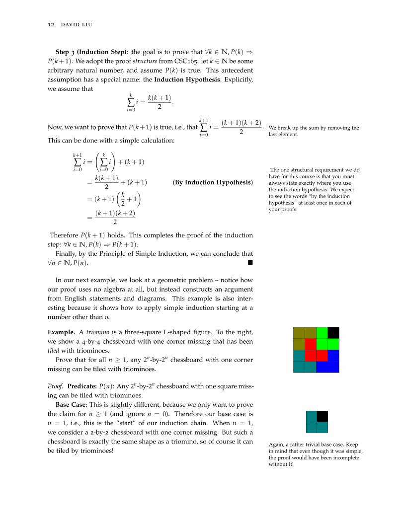
Example. A triomino is a three-square L-shaped figure. To the right,we show a 4-by-4 chessboard with one corner missing that has beentiled with triominoes.
Prove that for all n ≥ 1, any 2n-by-2n chessboard with one cornermissing can be tiled with triominoes.
Proof. Predicate: P(n): Any 2n-by-2n chessboard with one square miss-ing can be tiled with triominoes.
Base Case: This is slightly different, because we only want to provethe claim for n ≥ 1 (and ignore n = 0). Therefore our base case isn = 1, i.e., this is the “start” of our induction chain. When n = 1,we consider a 2-by-2 chessboard with one corner missing. But such achessboard is exactly the same shape as a triomino, so of course it canbe tiled by triominoes!
Again, a rather trivial base case. Keepin mind that even though it was simple,the proof would have been incompletewithout it!
introduction to the theory of computation 13
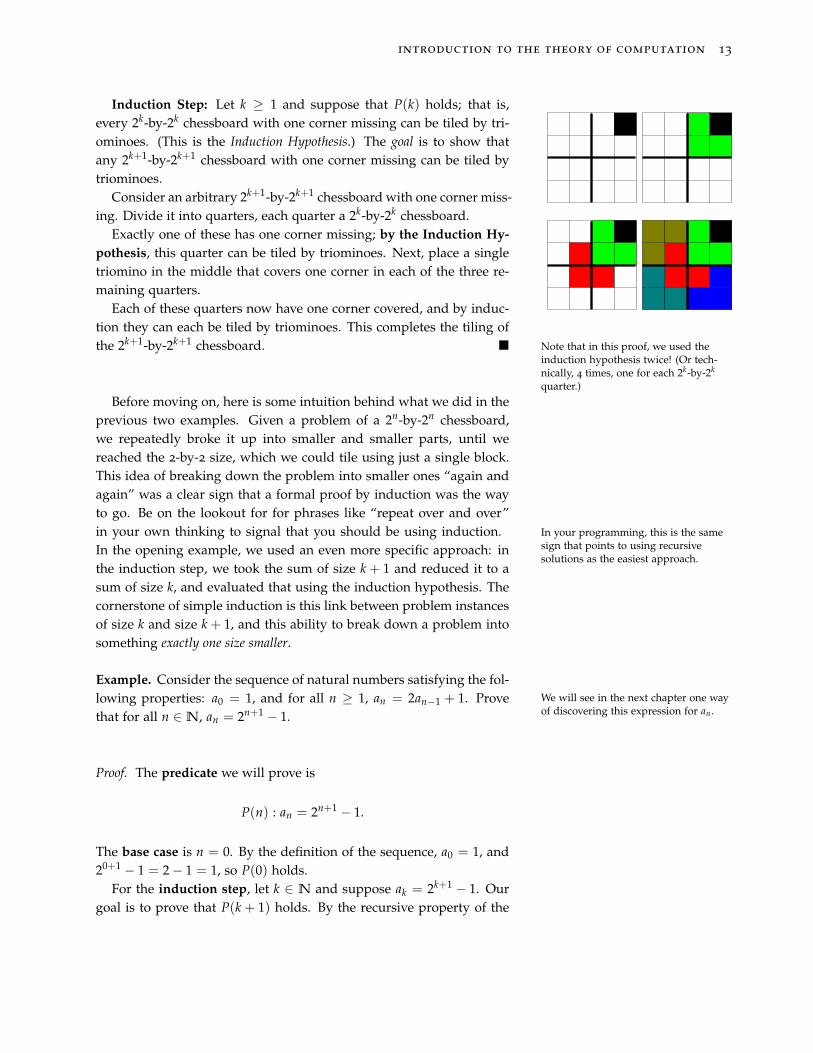
Induction Step: Let k ≥ 1 and suppose that P(k) holds; that is,every 2k-by-2k chessboard with one corner missing can be tiled by tri-ominoes. (This is the Induction Hypothesis.) The goal is to show thatany 2k+1-by-2k+1 chessboard with one corner missing can be tiled bytriominoes.
Consider an arbitrary 2k+1-by-2k+1 chessboard with one corner miss-ing. Divide it into quarters, each quarter a 2k-by-2k chessboard.
Exactly one of these has one corner missing; by the Induction Hy-pothesis, this quarter can be tiled by triominoes. Next, place a singletriomino in the middle that covers one corner in each of the three re-maining quarters.
Each of these quarters now have one corner covered, and by induc-tion they can each be tiled by triominoes. This completes the tiling ofthe 2k+1-by-2k+1 chessboard. � Note that in this proof, we used the
induction hypothesis twice! (Or tech-nically, 4 times, one for each 2k-by-2k
quarter.)
Before moving on, here is some intuition behind what we did in theprevious two examples. Given a problem of a 2n-by-2n chessboard,we repeatedly broke it up into smaller and smaller parts, until wereached the 2-by-2 size, which we could tile using just a single block.This idea of breaking down the problem into smaller ones “again andagain” was a clear sign that a formal proof by induction was the wayto go. Be on the lookout for for phrases like “repeat over and over”in your own thinking to signal that you should be using induction. In your programming, this is the same
sign that points to using recursivesolutions as the easiest approach.
In the opening example, we used an even more specific approach: inthe induction step, we took the sum of size k + 1 and reduced it to asum of size k, and evaluated that using the induction hypothesis. Thecornerstone of simple induction is this link between problem instancesof size k and size k + 1, and this ability to break down a problem intosomething exactly one size smaller.
Example. Consider the sequence of natural numbers satisfying the fol-lowing properties: a0 = 1, and for all n ≥ 1, an = 2an−1 + 1. Provethat for all n ∈N, an = 2n+1 − 1.
We will see in the next chapter one wayof discovering this expression for an.
Proof. The predicate we will prove is
P(n) : an = 2n+1 − 1.
The base case is n = 0. By the definition of the sequence, a0 = 1, and20+1 − 1 = 2− 1 = 1, so P(0) holds.
For the induction step, let k ∈ N and suppose ak = 2k+1 − 1. Ourgoal is to prove that P(k + 1) holds. By the recursive property of the
14 david liu
sequence,
ak+1 = 2ak + 1
= 2(2k+1 − 1) + 1 (by the I.H.)
= 2k+2 − 2 + 1
= 2k+2 − 1 �
When Simple Induction Isn’t Enough
By this point, you have done several examples using simple induc-tion. Recall that the intuition behind this proof technique is to reduceproblems of size k + 1 to problems of size k (where “size” might meanthe value of a number, or the size of a set, or the length of a string,etc.). However, for many problems there is no natural way to reduceproblem sizes just by 1. Consider, for example, the following problem:
Every prime can be written as a productof primes with just one multiplicand.
Prove that every natural number greater than 1 has a primefactorization, i.e., can be written as a product of primes.
How would you go about proving the induction step, using themethod we’ve done so far? That is, how would you prove P(k) ⇒P(k + 1)? This is a very hard question to answer, because even theprime factorizations of consecutive numbers can be completely differ-ent!
E.g., 210 = 2 · 3 · 5 · 7, but 211 is prime.
But if I asked you to solve this question by “breaking the problemdown,” you would come up with the idea that if k + 1 is not prime,then we can write k + 1 = a · b, where a, b < k + 1, and we can “do thisrecursively” until we’re left with a product of primes. Since we alwaysidentify recursion with induction, this hints at a more general form ofinduction that we can use to prove this statement.
Complete Induction
Recall the intuitive “chain of reasoning” that we do with simple in-duction: first we prove P(0), and then use P(0) to prove P(1), thenuse P(1) to prove P(2), etc. So when we get to k + 1, we try to proveP(k + 1) using P(k), but we have already gone through proving P(0),P(1), . . . , and P(k − 1)! In some sense, in Simple Induction we’rethrowing away all of our previous work and just using P(k). In Com-plete Induction, we keep this work and use it in our proof of the induc-tion step. Here is the formal statement of The Principle of CompleteInduction: complete induction(
P(0) ∧ ∀k,(
P(0) ∧ P(1) ∧ · · · ∧ P(k))⇒ P(k + 1)
)⇒ ∀n, P(n)

introduction to the theory of computation 15
The only difference between Complete and Simple Induction is inthe antecedent of the inductive part: instead of assuming just P(k), wenow assume all of P(0), P(1), . . . , P(k). Since these are assumptions weget to make in our proofs, Complete Induction proofs are often moreflexible than Simple Induction proofs – intuitively, because we have“more to work with.”
Somewhat surprisingly, everything wecan prove with Complete Inductionwe can also prove with Simple Induc-tion, and vice versa. So these prooftechniques are equally powerful.
Azadeh Farzan gave a great analogyfor the two types of induction. SimpleInduction is like an old man climbingstairs step by step; Complete Inductionis like a robot with multiple giantlegs, capable of jumping from anycombination of steps to a higher step.
Let’s illustrate this (slightly different) technique by proving the ear-lier claim about prime factorizations.
Example. Prove that every natural number greater than 1 has a primefactorization.
Proof. Predicate: P(n) : “There are primes p1, p2, . . . , pm (for some m ≥1) such that n = p1 p2 · · · pm.” We will show that ∀n ≥ 2, P(n).
Base Case: n = 2. Since 2 is prime, we can let p1 = 2 and say thatn = p1, so P(2) holds.
Induction Step: Here is the only structural difference for CompleteInduction proofs. We let k ≥ 2, and our Induction Hypothesis is nowto assume that for all 2 ≤ i ≤ k, P(i) holds. (That is, we’re assumingP(2), P(3), P(4), . . . , P(k).) The goal is still the same: prove that P(k +1) is true.
There are two cases. In the first case, assume k + 1 is prime. Thenof course k + 1 can be written as a product of primes, so P(k + 1) istrue. The product contains a single multipli-
cand, k + 1.In the second case, k + 1 is composite. But then by the definition ofcompositeness, there exist a, b ∈N such that k + 1 = ab and 2 ≤ a, b ≤k; that is, k + 1 has factors other than 1 and itself. This is the intuitionfrom earlier. And here is the “recursive thinking”: by the InductionHypothesis, P(a) and P(b) hold. Therefore we can write We can only use the Induction Hy-
pothesis because a and b are less thank + 1.a = q1 · · · ql1 and b = r1 · · · rl2 ,
where each of the q’s and r’s are prime. But then
k + 1 = ab = q1 · · · ql1 r1 · · · rl2 ,
and this is the prime factorization of k + 1. So P(k + 1) holds. �
Note that we used inductive thinking to break down the problem;but unlike Simple Induction, when we broke down the problem, wedidn’t know much about the sizes of the resulting problems, only thatthey were smaller than the original problem. Complete Induction al-lows us to handle this sort of problem.
Example. The Fibonacci sequence is a sequence of natural numbers de-fined recursively as f1 = f2 = 1, and for all n ≥ 3, fn = fn−1 + fn−2.
16 david liu
Prove that for all n ≥ 1,
fn =( 1+√
52 )n − ( 1−
√5
2 )n√
5.
Proof. Note that we really need complete induction here (and not justsimple induction) because fn is defined in terms of both fn−1 and fn−2,and not just fn−1 only.
The predicate we will prove is P(n) : fn =( 1+√
52 )n − ( 1−
√5
2 )n√
5. We
require two base cases: one for n = 1, and one for n = 2. These canbe checked by simple calculations:
( 1+√
52 )1 − ( 1−
√5
2 )1√
5=
1+√
52 − 1−
√5
2√5
=
√5√5
= 1 = f1
( 1+√
52 )2 − ( 1−
√5
2 )2√
5=
6+2√
54 − 6−2
√5
4√5
=
√5√5
= 1 = f2
For the induction step, let k ≥ 2 and assume P(1), P(2), . . . , P(k) hold.Consider fk+1. By the recursive definition, we have
fk+1 = fk + fk−1
=( 1+√
52 )k − ( 1−
√5
2 )k√
5+
( 1+√
52 )k−1 − ( 1−
√5
2 )k−1√
5(by I.H.)
=( 1+√
52 )k + ( 1+
√5
2 )k−1√
5−
( 1−√
52 )k + ( 1−
√5
2 )k−1√
5
=( 1+√
52 )k−1( 1+
√5
2 + 1)√5
−( 1−√
52 )k−1( 1−
√5
2 + 1)√5
=( 1+√
52 )k−1 · 6+2
√5
4√5
−( 1−√
52 )k−1 · 6−2
√5
4√5
=( 1+√
52 )k−1( 1+
√5
2 )2√
5−
( 1−√
52 )k−1( 1−
√5
2 )2√
5
=( 1+√
52 )k+1√
5−
( 1−√
52 )k+1√
5�
introduction to the theory of computation 17
Beyond Numbers
So far, our proofs have all been centred on natural numbers. Even insituations where we have proved statements about other objects – likesets and chessboards – our proofs have always required associatingthese objects with natural numbers. Consider the following problem:
Prove that any non-empty binary tree has exactly one morenode than edge.
We could use either simple or complete induction on this problemby associating every tree with a natural number (height and numberof nodes are two of the most common). But this is not the most “nat-ural” way of approaching this problem (though it’s perfectly valid!)because binary trees already have a lot of nice recursive structure thatwe should be able to use directly, without shoehorning in natural num-bers. What we want is a way of proving statements about objects otherthan numbers. Thus we move away from the set of natural numbers N
to more general sets, such as the set of all non-empty binary trees.
Recursive Definitions of Sets
You are already familiar with many descriptions of sets: {2, π,√
10},{x ∈ R | x ≥ 4.5}, and “the set of all non-empty binary trees” are allperfectly valid descriptions of sets. Unfortunately, these set descrip-tions don’t lend themselves very well to induction, because inductionis recursion and it isn’t clear how to apply recursive thinking to any ofthese descriptions. However, for some objects - like binary trees - it isrelatively straightforward to define them recursively. As a warm-up,consider the following way of describing the set of natural numbers.
Example. Suppose we want to construct a recursive definition of N.Here is one way. Define N to be the (smallest) set such that:
The “smallest” means that nothing elseis in N. This is an important point tomake; for example, the set of integersZ also satisfies (B1) and (R1). In therecursive definitions below, we omit“smallest” but it is always implicitlythere.
• 0 ∈N
• If k ∈N, then k + 1 ∈N
Notice how similar this definition looks to the principle of simpleinduction! Induction fundamentally makes use of this recursive struc-ture of N. We’ll refer to the first rule as the base of the definition, andsecond as the recursive rule. In general, a recursive definition can havemultiple base and recursive rules!
Example. Construct a recursive definition of “the set of all non-emptybinary trees.”
18 david liu
Intuitively, the base rule(s) always capture the smallest or simplestelements of a set. Certainly the smallest non-empty binary tree is asingle node.
What about larger trees? This is where “breaking down” problemsinto smaller subproblems makes the most sense. You should knowfrom CSC148 that we really store binary trees in a recursive manner:every tree has a root node, then links to the roots of the left and rightsubtrees (the suggestive word here is “subtree.”) One slight subtletyis that either one of these could be empty. Here is a formal recursivedefinition (before you read it, try coming up with one yourself!):
• A single node is a non-empty binary tree.
• If T1, T2 are two non-empty binary trees, then the tree with a newroot r connected to the roots of T1 and T2 is a non-empty binarytree.
• If T1 is a non-empty binary tree, then the tree with a new root rconnected to the root of T1 to the left or to the right is a non-emptybinary tree.
We’ll treat these as two separate cases,following the traditional applicationof binary trees in computer science.However, from a graph theoretic pointof view, these two trees are isomorphicto each other.
Structural Induction
Now, we mimic the format of our induction proofs, but with the recur-sive definition of non-empty binary trees rather than natural numbers.The similarity of form is why this type of proof is called structuralinduction. In particular, notice the identical terminology. structural induction
Example. Prove that every non-empty binary tree has one more nodethan edge.
Proof. As before, we need to define a predicate to nail down exactlywhat it is we’d like to prove. However, unlike all of the previouspredicates we’ve seen, which have been boolean functions on naturalnumbers, now the domain of the predicate in this case is the set of allnon-empty binary trees.
Predicate: P(T): T has one more node than edge.
We will use induction to prove that for every non-empty binary treeT, P(T) holds.
Note that here the domain of the pred-icate is NOT N, but instead the set ofnon-empty binary trees.
Base Case: Our base case is determined by the first rule. SupposeT is a single node. Then it has one node and no edges, so P(T) holds.
Induction Step: We’ll divide our proof into two parts, one for eachrecursive rule.
• Let T1 and T2 be two non-empty binary trees, and assume P(T1)
and P(T2) hold. (This is the induction hypothesis.) Let T be the tree
introduction to the theory of computation 19
constructed by attaching a node r to the roots of T1 and T2. LetV(G) and E(G) denote the number of nodes and edges in a tree G,respectively. Then we have the equations
V(T) = V(T1) + V(T2) + 1
E(T) = E(T1) + E(T2) + 2
since one extra node (new root r) and two extra edges (from r tothe roots of T1 and T2) were added to form T. By the inductionhypothesis, V(T1) = E(T1) + 1 and V(T2) = E(T2) + 1, and so
V(T) = E(T1) + 1 + E(T2) + 1 + 1
= E(T1) + E(T2) + 3
= E(T) + 1
Therefore P(T) holds.
• Let T1 be a non-empty binary tree, and suppose P(T1) holds. Let Tbe the tree formed by taking a new node r and adding and edge tothe root of T1. Then V(T) = V(T1) + 1 and E(T) = E(T1) + 1, andsince V(T1) = E(T1) + 1 (by the induction hypothesis), we have
V(T) = E(T1) + 2 = E(T) + 1. �
In structural induction, we identify some property that is satisfiedby the simplest (base) elements of the set, and then show that theproperty is preserved under each of the recursive construction rules.
We say that such a property is invariantunder the recursive rules, meaningit isn’t affected when the rules areapplied. The term “invariant” willreappear throughout this course indifferent contexts.
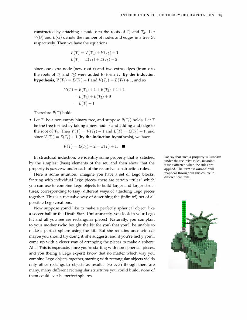
Here is some intuition: imagine you have a set of Lego blocks.Starting with individual Lego pieces, there are certain “rules” whichyou can use to combine Lego objects to build larger and larger struc-tures, corresponding to (say) different ways of attaching Lego piecestogether. This is a recursive way of describing the (infinite!) set of allpossible Lego creations.
Now suppose you’d like to make a perfectly spherical object, likea soccer ball or the Death Star. Unfortunately, you look in your Legokit and all you see are rectangular pieces! Naturally, you complainto your mother (who bought the kit for you) that you’ll be unable tomake a perfect sphere using the kit. But she remains unconvinced:maybe you should try doing it, she suggests, and if you’re lucky you’llcome up with a clever way of arranging the pieces to make a sphere.Aha! This is impossible, since you’re starting with non-spherical pieces,and you (being a Lego expert) know that no matter which way youcombine Lego objects together, starting with rectangular objects yieldsonly other rectangular objects as results. So even though there aremany, many different rectangular structures you could build, none ofthem could ever be perfect spheres.
20 david liu
A Larger Example
Let us turn our attention to another useful example of induction: prov-ing the equivalence of recursive and non-recursive definitions. Weknow from our study of Python that often problems can be solvedusing either recursive or iterative programs, but we’ve taken it for Although often a particular problem
lends itself more to one technique orthe other.
granted that these programs really can accomplish the same task. We’lllook later in this course at proving things about what programs do, butfor a warm-up in this section, we’ll step back from programs and provea similar mathematical result.
Example. Consider the following recursively defined set S ⊆N2:
• (0, 0) ∈ S
• If (a, b) ∈ S, then so are (a + 1, b + 1) and (a + 3, b) Note that there are really two recursiverules here.
Also, define the set S′ = {(x, y) ∈ N2 | x ≥ y ∧ 3 | x− y}. Prove that Here, 3 | x− y means 3 divides x− y.
these two definitions are equivalent, i.e., S = S′.
Proof. We divide our solution into two parts. First, we show thatS ⊆ S′, that is, every element of S satisfies the property of S′, usingstructural induction. Then, we prove using complete induction thatevery element of S′ can be constructed from the recursive rules of S.
Part 1: S ⊆ S′. For clarity, we define the predicate
P(x, y) : x ≥ y ∧ 3 | x− y
The only base case is (0, 0). Clearly, P(0, 0) is true, as 0 ≥ 0 and 3 | 0.Now for the induction step, there are two recursive rule. Let (a, b) ∈
S, and suppose P(a, b) holds. Consider (a + 1, b + 1). By the induction P(a, b) : a ≥ b ∧ 3 | a− b.
hypothesis, a ≥ b, and so a+ 1 ≥ b+ 1. Also, (a− 1)− (b− 1) = a− b,which is divisible by 3 (by the I.H.). So P(a + 1, b + 1) also holds.
Finally, consider (a + 3, b). Since a ≥ b (by the I.H.), a + 3 ≥ b. Also,since 3 | a− b, we can let a− b = 3k. Then (a + 3)− b = 3(k + 1), so3 | (a + 3)− b, and hence P(a + 3, b) holds.
Part 2: S′ ⊆ S. We would like to use complete induction, but we canonly apply this technique to natural numbers, and not pairs of naturalnumbers. So we need to associate each pair (a, b) with a single naturalnumber. We can do this by considering the sum of the pair. We definethe following predicate:
P(n) : for every (x, y) ∈ S′ such that x + y = n, (x, y) ∈ S.
It should be clear that proving ∀n ∈ N, P(n) is equivalent to provingthat S′ ⊆ S. We will prove the former using complete induction.
The base case is n = 0. the only element of S′ we need to consideris (0, 0), which is certainly in S by the base rule of the definition.
introduction to the theory of computation 21
Now let k ∈ N, and suppose P(0), P(1), . . . , P(k) all hold. Let(x, y) ∈ S′ such that x + y = k + 1. We will prove that (x, y) ∈ S.There are two cases to consider:
• y > 0. Then since x ≥ y, x > 0. Then (x− 1, y− 1) ∈ S′, and (x− The ≥ 0 checks ensure that x, y ∈N.
1) + (y − 1) = k − 1. By the Induction Hypothesis (in particular,P(k − 1)), (x − 1, y − 1) ∈ S. then (x, y) ∈ S by applying the firstrecursive rule in the definition of S.
• y = 0. Since k + 1 > 0, it must be the case that x 6= 0. Then sincex − y = x, x must be divisible by 3, and so x ≥ 3. Then (x −3, y) ∈ S′ and (x + 3) + y = k− 3, so by the Induction Hypothesis,(x− 3, y) ∈ S. Applying the second recursive rule in the definitionshows that (x, y) ∈ S. �
Exercises
1. Prove that for all n ∈N,
n
∑i=0
i2 =n(n + 1)(2n + 1)
6.
2. Let a ∈ R, a 6= 1. Prove that for all n ∈N,
n
∑i=0
ai =an+1 − 1
a− 1.
3. Prove that for all n ≥ 1,
n
∑k=1
1k(k + 1)
=n
n + 1.
4. Prove that ∀n ∈N, the units digit of 4n is either 1, 4, or 6.
5. Prove that ∀n ∈ N, 3 | 4n − 1, where “m | n” means that m dividesn, or equivalently that n is a multiple of m. This can be expressedalgebraically as ∃k ∈N, n = mk.
6. Prove that for all n ≥ 2, 2n + 3n < 4n.
7. Let m ∈N. Prove that for all n ∈N, m | (m + 1)n − 1.
8. Prove that ∀n ∈ N, n2 ≤ 2n + 1. Hint: first prove, without usinginduction, that 2n + 1 ≤ n2 − 1 for n ≥ 3.
9. Find a natural number k ∈ N such that for all n ≥ k, n3 + n < 3n.Then, prove this result using simple induction.
10. Prove that 3n < n! for all n > 6.
11. Prove that for every n ∈N, every set of size n has exactly 2n subsets.

22 david liu
12. Find formulas for the number of even-sized subsets and odd-sizedsubsets of a set of size n. Prove that your formulas are correct in asingle induction argument. So your predicate should be something
like “every set of size n has ... even-sized subsets and ... odd-sized subsets.”
13. Prove, using either simple or complete induction, that any binarystring begins and ends with the same character if and only if it con- A binary string is a string containing
only 0’s and 1’s.tains an even number of occurrences of substrings from {01, 10}.14. A ternary tree is a tree where each node has at most 3 children. Prove
that for every n ≥ 1, every non-empty ternary tree of height n hasat most 3n − 2 nodes.
15. Let a ∈ R, a 6= 1. Prove that for all n ∈N,
n
∑i=0
i · ai =n · an+2 − (n + 1) · an+1 + a
(a− 1)2 .
Challenge: can you mathematically derive this formula by startingfrom the standard geometric identity?
16. Recall two standard trigonometric identities:
cos(x + y) = cos(x) cos(y)− sin(x) sin(y)
sin(x + y) = sin(x) cos(y) + cos(x) sin(y)
Also recall the definition of the imaginary number i =√−1. Prove,
using induction, that
(cos(x) + i sin(x))n = cos(nx) + i sin(nx).
17. The Fibonacci sequence is an infinite sequence of natural numbersf1, f2, . . . with the following recursive definition:
fi =
{1, if i = 1, 2
fi−1 + fi−2, if i > 2
(a) Prove that for all n ≥ 1,n
∑i=1
fi = fn+2 − 1.
(b) Prove that for all n ≥ 1,n
∑i=1
f2i−1 = f2n.
(c) Prove that for all n ≥ 2, F2n − Fn+1Fn−1 = (−1)n−1.
(d) Prove that for all n ≥ 1, gcd( fn, fn+1) = 1. You may use the fact that for all a < b,gcd(a, b) = gcd(a, b− a).
(e) Prove that for all n ≥ 1,n
∑i=1
f 2i = fn fn+1.
18. A full binary tree is a non-empty binary tree where every node hasexactly 0 or 2 children. Equivalently, every internal node (non-leaf)has exactly two children.
(a) Prove using complete induction that every full binary tree has anodd number of nodes. You can choose to do induction on
either the height or number of nodesin the tree. A solution with simpleinduction is also possible, but lessgeneralizable.

introduction to the theory of computation 23
(b) Prove using complete induction that every full binary tree hasexactly one more leaf than internal nodes.
(c) Give a recursive definition for the set of all full binary trees.(d) Prove questions 1 & 2 using structural induction instead of com-
plete induction.
19. Consider the sets of binary trees with the following property: foreach node, the heights of its left and right children differ by at most1. Prove that every binary tree with this property of height n has atleast (1.5)n − 1 nodes.
20. Let k > 1. Prove that for all n ∈N, 1− jk≤(
1− 1k
)n.
21. Consider the following recursively defined function f : N→N.
f (n) =
2, if n = 0
7, if n = 1
( f (n− 1))2 − f (n− 2), if n ≥ 2
Prove that for all n ∈ N, 3 | f (n)− 2. It will be helpful to phraseyour predicate here as ∃k ∈N, f (n) = 3k + 2.
22. Prove that every natural number greater than 1 can be written asthe sum of prime numbers.
23. We define the set S of strings over the alphabet {[, ]} recursively by
• ε, the empty string, is in S
• If w ∈ S, then so is [w]
• If x, y ∈ S, then so is xy
Prove that every string in S is balanced, i.e., the number of left brack-ets equals the number of right brackets.
24. The Fibonacci trees Tn are a special set of binary trees defined recur-sively as follows.
• T1 and T2 are binary trees with only a single vertex.
• For n > 2, Tn consists of a root node whose left subtree is Tn−1,and right subtree is Tn−2.
(a) Prove that for all n ≥ 2, the height of Tn is n− 2.
(b) Prove that for all n ≥ 1, Tn has fn nodes, where fn is the n-thFibonacci number.
25. Consider the following recursively defined set S ⊂ N 2.
• 2 ∈ S
• If k ∈ S, then k2 ∈ S
• If k ∈ S, and k ≥ 2, thenk2∈ S
(a) Prove that every element of S is a power of 2, i.e., can be writtenin the form 2m for some m ∈N.

24 david liu
(b) Prove that every power of 2 (including 20) is in S.
26. Consider the set S ⊂ N2 of ordered pair of integers defined by thefollowing recursive definition:
• (3, 2) ∈ S
• If (x, y) ∈ S, then (3x− 2y, x) ∈ S
Also consider the set S′ ⊂ N2 with the following non-recursivedefinition:
S′ = {(2k+1 + 1, 2k + 1) | k ∈N}.
Prove that S = S′, or in other words, that the recursive and non-recursive definitions agree.
27. We define the set of propositional formulas PF as follows:
• Any proposition P is a propositional formula.
• If F is a propositional formula, then so is ¬F.
• If F1 and F2 are propositional formulas, then so are F1∧ F2, F1∨ F2,F1 ⇒ F2, and F1 ⇔ F2.
Prove that for all propositional formulas F, F has a logically equiv-alent formula G such that G only has negations applied to proposi-tions. For example, we have the equivalence
¬(¬(P ∧Q)⇒ R)⇐⇒ (¬P ∨ ¬Q) ∧ ¬R
Hint: you won’t have much luck applying induction directly tothe statement in the question. (Try it!) Instead, prove the strongerstatement: “F and ¬F have equivalent formulas that only have nega-tions applied to propositions.”
28. It is well-known that Facebook friendships are the most importantrelationships you will have in your lifetime. For a person x on Face-book, let fx denote the number of friends x has. Find a relationshipbetween the total number of Facebook friendships in the world, andthe sum of all of the fx’s (over every person on Facebook). Proveyour relationship using induction.
29. Consider the following 1-player game. We start with n pebbles ina pile, where n ≥ 1. A valid move is the following: pick a pile withmore than 1 pebble, and divide it into two smaller piles. When thishappens, add to your score the product of the sizes of the two newpiles. Continue making moves until no more can be made, i.e., thereare n piles each containing a single pebble.
Prove using complete induction that no matter how the player
makes her moves, she will always scoren(n− 1)
2points when play-
ing this game with n pebbles. So this game is completely determinedby the starting conditions, and not at allby the player’s choices. Sounds fun.
30. A certain summer game is played with n people, each carrying onewater balloon. The players walk around randomly on a field until
introduction to the theory of computation 25
a buzzer sounds, at which point they stop. You may assume thatwhen the buzzer sounds, each player has a unique closest neigh-bour. After stopping, each player then throws his water balloon attheir closest neighbour. The winners of the game are the playerswho are dry after the water balloons have been thrown (assumeeveryone has perfect aim).
Prove that for every odd n, this game always has at least onewinner.
The following problems are for the more mathematically-inclinedstudents.
1. The Principle of Double Induction is as follows. Suppose that P(x, y)is a predicate with domain N2 satisfying the following properties:
(1) P(0, y) holds for all y ∈N
(2) For all (x, y) ∈N2, if P(x, y) holds, then so does P(x + 1, y).
Then we may conclude that for all x, y ∈N, P(x, y).
Prove that the Principle of Double Induction is equivalent to thePrinciple of Simple Induction.
2. Prove that for all n ≥ 1, and positive real numbers x1, . . . , xn ∈ R+,
1− x1
1 + x1· 1− x2
1 + x2· · · · 1− xn
1 + xn≥ 1− S
1 + S,
where S =n
∑i=1
xi.
3. A unit fraction is a fraction of the form1n
, n ∈ Z+. Prove that every
rational number 0 <pq
< 1 can be written as the sum of distinct
unit fractions.


Recursion
Now, programming! In this chapter, we will apply what we’ve learnedabout induction to study recursive algorithms. In particular, we willlearn how to analyse the time complexity of recursive programs, forwhich the runtime on an input of size n depends on the runtime onsmaller inputs. Unsurprisingly, this is tightly connected to the studyof recursively defined (mathematical) functions; we will discuss howto go from a recurrence relation like f (n + 1) = f (n) + f (n − 1) toa closed form expression like f (n) = 2n + n2. For recurrences of aspecial form, we will see how the Master Theorem gives us immediate,tight asymptotic bounds. These recurrences will be used for divide- Recall that asymptotic bounds involve
Big-O, and are less precise than exactexpressions.
and-conquer algorithms; you will gain experience with this commonalgorithmic paradigm and even design algorithms of your own.
Measuring Runtime
Recall that one of the most important properties of an algorithm is howlong it takes to run. We can use the number of steps as a measurementof running time; but reporting an absolute number like “10 steps” or“1 000 000 steps” an algorithm takes is pretty meaningless unless weknow how “big” the input was, since of course we’d expect algorithmsto take longer on larger inputs. You may recall that input size is for-
mally defined as the number of bitsrequired to represent the input. In thiscourse, we’ll be dealing mainly withlists, and the approximation of theirsize as simply their length.
So a more meaningful measure of runtime is “10 steps when the in-put has size 2” or “1 000 000 steps when the input has size 300” or evenbetter, “n2 + 2 steps when the input has size n.” But as you probablyremember from CSC165, counting an exact number of steps is oftentedious and arbitrary, so we care more about the Big-O (asymptotic)analysis of an algorithm. In this course, we will mainly care
about the upper bound on the worst-case runtime of algorithms; that is, theabsolute longest an algorithm could runon a given input size n.
In CSC165 you mastered analysing the runtime of iterative algo-rithms. As we’ve mentioned several times by now, induction is verysimilar to recursion; since induction has been the key idea of the courseso far, it should come as no surprise that we’ll turn our attention to re-cursive algorithms now!

28 david liu
A Simple Recursive Function
Consider the following simple recursive function, which you probablysaw in CSC148:
All code in this course will be inPython-like pseudocode, which meansthe syntax and methods will be mostlyPythonic, with some English makingthe code more readable and/or in-tuitive. We’ll expect you to follow asimilar style.
1 def fact(n):
2 if n == 1:
3 return 1
4 else:
5 return n * fact(n-1)
In CSC148, it was surely claimed thatthis function computes n! We’ll see laterin this course how to formally prove thatis what this function does.
How would you informally analyse the runtime of this algorithm?One might say that the recursion depth is n, and at each call thereis just one step other than the recursive call, so the runtime is O(n),i.e., linear time. But in performing a step-by-step analysis, we reach astumbling block with the recursive call fact(n-1): the runtime of facton input n depends on its runtime on input n − 1! Let’s see how todeal with the relationship, using mathematics and induction.
Recursively Defined Functions
You should all be familiar with standard function notation: f (n) = n2,f (n) = n log n, or the slightly more unusual (but no less meaningful)f (n) = “the number of distinct prime factors of n.” There is a secondway of defining functions using recursion, e.g.,
f (n) =
{0, if n = 0
f (n− 1) + 2n− 1, if n ≥ 1
Recursive definitions allow us to capture marginal or relative differ- recursively defined function
ence between function values, even when we don’t know their exactvalues. But recursive definitions have a significant downside: we canonly calculate large values of f by computing smaller values first. Forcalculating extremely large, or symbolic values of f (like f (n2 + 3n)), arecursive definition is inadequate; what we would really like is a closedform expression for f , one that doesn’t depend on other values of f . Inthis case, the closed form expression for f is f (n) = n2. You will prove this in the Exercises.
Before returning to our earlier example, let us see how to apply thisto a more concrete example.
Example. There are exactly two ways of tiling a 3-by-2 grid using tri-ominoes, shown to the right:
Develop a recursive definition for f (n), the number of ways of tilinga 3-by-n grid using triominoes for n ≥ 1. Then, find a closed formexpression for f .
Solution:
introduction to the theory of computation 29
Note that if n = 1, there are no possible tilings, since no triominowill fit in a 3-by-1 board. We have already observed that there are 2
tilings for n = 2. Suppose n > 2. The key idea to get a recurrenceis that for a 3-by-n block, first consider the upper-left square. In anytiling, there are only two possible triomino placements that can coverit (these orientations are shown in the diagram above. Once we havefixed one of these orientations, there is only one possible triominoorientation that can cover the bottom-left square (again, these are thetwo orientations shown in the figure).
So there are exactly two possibilities for covering both the bottom-left and top-left squares. But once we’ve put these two down, we’vetiled the leftmost 3-by-2 part of the grid, and the remainder of the tilingreally just tiles the remaining 3-by-(n − 2) part of the grid; there aref (n− 2) such tilings. Since these two parts are independent of each Because we’ve expressed f (n) in terms
of f (n− 2), we need two base cases –otherwise, at n = 2 we would be stuck,as f (0) is undefined.
other, we get the total number of tilings by multiplying the number ofpossibilities for each. Therefore the recurrence relation is:
f (n) =
0, if n = 1
2, if n = 2
2 f (n− 2), if n > 2
Now that we have the recursive definition of f , we would like to findits closed form expression. The first step is to guess the closed formexpression, by a “brute force” approach known as repeated substitution.Intuitively, we’ll expand out the recursive definition until we find apattern. So much of mathematics is finding
patterns.
f (n) = 2 f (n− 2)
= 4 f (n− 4)
= 8 f (n− 6)
...
= 2k f (n− 2k)
There are two possibilities. If n is odd, say n = 2m + 1, then we havef (n) = 2m f (1) = 0, since f (1) = 0. If n is even, say n = 2m, thenf (n) = 2m−1 f (2) = 2m−1 · 2 = 2m. Writing our final answer in termsof n only:
f (n) =
{0, if n is odd
2n2 , if n is even
Thus we’ve obtained the closed form formula f (n) – except the... in
our repeated substitution does not constitute a formal proof! When
you saw the..., you probably interpreted it as “repeat over and over
30 david liu
again until. . . ” and we already know how to make this thinking for-mal: induction! That is, given the recursive definition of f , we can proveusing complete induction that f (n) has the closed form given above.
Why complete and not simple induc-tion? We need the induction hypothesisto work for n− 2, and not just n− 1.
This is a rather straightforward argument, and we leave it for the Ex-ercises.
We will now apply this technique to our earlier example.
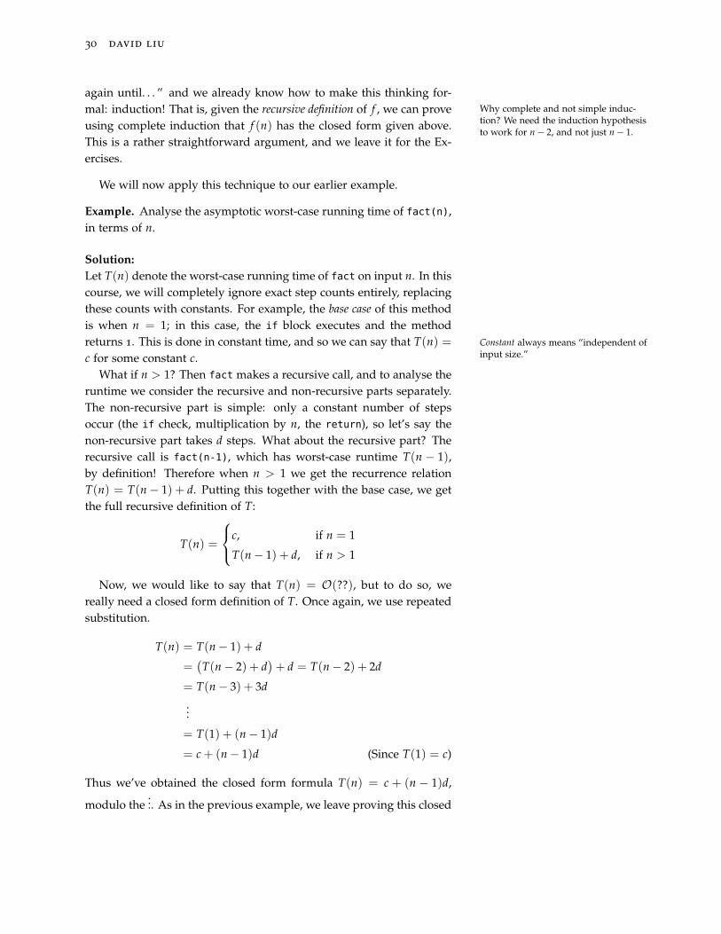
Example. Analyse the asymptotic worst-case running time of fact(n),in terms of n.
Solution:Let T(n) denote the worst-case running time of fact on input n. In thiscourse, we will completely ignore exact step counts entirely, replacingthese counts with constants. For example, the base case of this methodis when n = 1; in this case, the if block executes and the methodreturns 1. This is done in constant time, and so we can say that T(n) = Constant always means “independent of
input size.”c for some constant c.What if n > 1? Then fact makes a recursive call, and to analyse the
runtime we consider the recursive and non-recursive parts separately.The non-recursive part is simple: only a constant number of stepsoccur (the if check, multiplication by n, the return), so let’s say thenon-recursive part takes d steps. What about the recursive part? Therecursive call is fact(n-1), which has worst-case runtime T(n − 1),by definition! Therefore when n > 1 we get the recurrence relationT(n) = T(n− 1) + d. Putting this together with the base case, we getthe full recursive definition of T:
T(n) =
c, if n = 1
T(n− 1) + d, if n > 1
Now, we would like to say that T(n) = O(??), but to do so, wereally need a closed form definition of T. Once again, we use repeatedsubstitution.
T(n) = T(n− 1) + d
=(T(n− 2) + d
)+ d = T(n− 2) + 2d
= T(n− 3) + 3d...
= T(1) + (n− 1)d
= c + (n− 1)d (Since T(1) = c)
Thus we’ve obtained the closed form formula T(n) = c + (n − 1)d,
modulo the.... As in the previous example, we leave proving this closed
introduction to the theory of computation 31
form as an example. Exercise: prove that for all n ≥ 1, T(n) = c +(n− 1)d.
After proving this closed form, the final step is simply to convertthis closed form into an asymptotic bound on T. Since c and d areconstants with respect to n, we have that T(n) = O(n).
Now let’s see a more complicated recursive function.
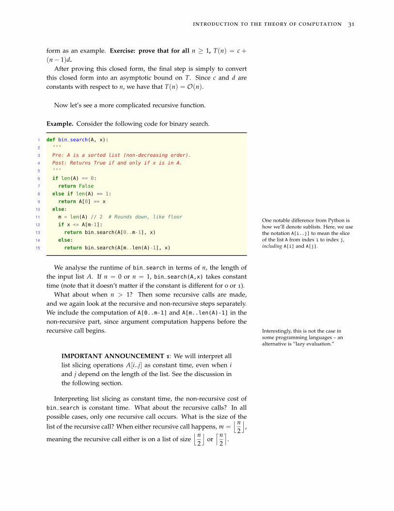
Example. Consider the following code for binary search.
1 def bin_search(A, x):
2 ’’’
3 Pre: A is a sorted list (non-decreasing order).
4 Post: Returns True if and only if x is in A.
5 ’’’
6 if len(A) == 0:
7 return False
8 else if len(A) == 1:
9 return A[0] == x
10 else:
11 m = len(A) // 2 # Rounds down, like floor
12 if x <= A[m-1]:
13 return bin_search(A[0..m-1], x)
14 else:
15 return bin_search(A[m..len(A)-1], x)
One notable difference from Python ishow we’ll denote sublists. Here, we usethe notation A[i..j] to mean the sliceof the list A from index i to index j,including A[i] and A[j].
We analyse the runtime of bin_search in terms of n, the length ofthe input list A. If n = 0 or n = 1, bin_search(A,x) takes constanttime (note that it doesn’t matter if the constant is different for 0 or 1).
What about when n > 1? Then some recursive calls are made,and we again look at the recursive and non-recursive steps separately.We include the computation of A[0..m-1] and A[m..len(A)-1] in thenon-recursive part, since argument computation happens before therecursive call begins. Interestingly, this is not the case in
some programming languages – analternative is “lazy evaluation.”
IMPORTANT ANNOUNCEMENT 1: We will interpret alllist slicing operations A[i..j] as constant time, even when iand j depend on the length of the list. See the discussion inthe following section.
Interpreting list slicing as constant time, the non-recursive cost ofbin_search is constant time. What about the recursive calls? In allpossible cases, only one recursive call occurs. What is the size of the
list of the recursive call? When either recursive call happens, m =⌊n
2
⌋,
meaning the recursive call either is on a list of size⌊n
2
⌋or⌈n
2
⌉.

32 david liu
IMPORTANT ANNOUNCEMENT 2: In this course, wewon’t care about floors and ceilings. We’ll always assumethat the input sizes are “nice” so that the recursive calls al-ways divides the list evenly. In the case of binary search,we’ll assume that n is a power of 2.
You may look in Vassos Hadzilacos’course notes for a complete handlingof floors and ceilings. The algebra isa little more involved, and the bottomline is that they don’t change theasymptotic analysis.
With this in mind, we conclude that the recurrence relation for T(n)is T(n) = T
(n2
)+ d. Therefore the full recursive definition of T is
T(n) =
c, if n ≤ 1
T(n
2
)+ d, if n > 1 Again, we omit floors and ceilings.
Let us use repeated substitution to guess a closed form. Assumethat n = 2k for some natural number k.
T(n) = T(n
2
)+ d
=(
T(n
4
)+ d)+ d = T
(n4
)+ 2d
= T(n
8
)+ 3d
...
= T( n
2k
)+ kd
= T(1) + kd (Since n = 2k)
= c + kd (Since T(1) = c)
Once again, we’ll leave proving this closed form to the Exercises. SoT(n) = c + kd. This expression is quite misleading, because it seemsto not involve an n, and hence be constant time – which we know isnot the case for binary search! The key is to remember that n = 2k,so k = log2 n. Therefore we have T(n) = c + d log2 n, and so T(n) =
O(log n).
Aside: List Slicing vs. Indexing
In our analysis of binary search, we assumed that the list slicing op-eration A[0..m-1] took constant time. However, this is not the casein Python and many other programming languages, which implementthis operation by copying the sliced elements into a new list. Depend-ing on the scale of your application, this can be undesirable for tworeasons: this copying take time linear in the size of the slice, and useslinear additional memory.
While we are not so concerned in this course about the second is-sue, the first can drastically change our runtime analysis (e.g., in our
introduction to the theory of computation 33
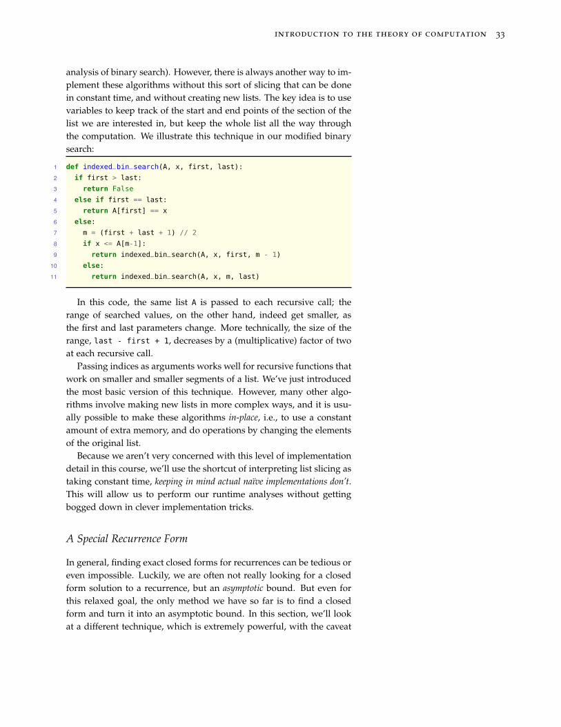
analysis of binary search). However, there is always another way to im-plement these algorithms without this sort of slicing that can be donein constant time, and without creating new lists. The key idea is to usevariables to keep track of the start and end points of the section of thelist we are interested in, but keep the whole list all the way throughthe computation. We illustrate this technique in our modified binarysearch:
1 def indexed_bin_search(A, x, first, last):
2 if first > last:
3 return False
4 else if first == last:
5 return A[first] == x
6 else:
7 m = (first + last + 1) // 2
8 if x <= A[m-1]:
9 return indexed_bin_search(A, x, first, m - 1)
10 else:
11 return indexed_bin_search(A, x, m, last)
In this code, the same list A is passed to each recursive call; therange of searched values, on the other hand, indeed get smaller, asthe first and last parameters change. More technically, the size of therange, last - first + 1, decreases by a (multiplicative) factor of twoat each recursive call.
Passing indices as arguments works well for recursive functions thatwork on smaller and smaller segments of a list. We’ve just introducedthe most basic version of this technique. However, many other algo-rithms involve making new lists in more complex ways, and it is usu-ally possible to make these algorithms in-place, i.e., to use a constantamount of extra memory, and do operations by changing the elementsof the original list.
Because we aren’t very concerned with this level of implementationdetail in this course, we’ll use the shortcut of interpreting list slicing astaking constant time, keeping in mind actual naïve implementations don’t.This will allow us to perform our runtime analyses without gettingbogged down in clever implementation tricks.
A Special Recurrence Form
In general, finding exact closed forms for recurrences can be tedious oreven impossible. Luckily, we are often not really looking for a closedform solution to a recurrence, but an asymptotic bound. But even forthis relaxed goal, the only method we have so far is to find a closedform and turn it into an asymptotic bound. In this section, we’ll lookat a different technique, which is extremely powerful, with the caveat

34 david liu
that it works only for a special recurrence form.We can motivate this recurrence form by considering a style of re-
cursive algorithm called divide-and-conquer. We’ll discuss this in detailin the next section, but for now consider the mergesort algorithm, mergesort
which can roughly be outlined in three steps:
1. Divide the list into two equal halves.
2. Sort each half separately, using recursive calls to mergesort.
3. Merge each of the sorted halves.
1 def mergesort(A):
2 if len(A) == 1:
3 return A
4 else:
5 m = len(A) // 2
6 L1 = mergesort(A[0..m-1])
7 L2 = mergesort(A[m..len(A)-1])
8 return merge(L1, L2)
9 def merge(A, B):
10 i = 0
11 j = 0
12 C = []
13 while i < len(A) and j < len(B):
14 if A[i] <= B[j]:
15 C.append(A[i]) # Add A[i] to the end of C
16 i += 1
17 else:
18 C.append(B[j])
19 j += 1
20 return C + A[i..len(A)-1] + B[j..len(B)-1] # List concatenation
Consider the analysis of T(n), the runtime of mergesort(A) wherelen(A) = n. Steps 1 and 3 together take linear time. What about Step Careful implementations of mergesort
can do step 1 in constant time, butmerging always takes linear time.
2? Since this is recursive step, we’d expect T to appear here. There aretwo fundamental questions:
• What is the size of each recursive call?
• What is the size of the argument lists passed to the recusive calls?
From the written description, you should be able to intuit that there
are two recursive calls, each on a list of sizen2
. So the cost of Step 2 is For the last time, we’ll point out that weignore floors and ceilings.
2T(n
2
). Putting all three steps together, we get a recurrence relation
T(n) = 2T(n
2
)+ cn.
This is an example of our special recurrence form:
T(n) = aT(n
b
)+ f (n),
introduction to the theory of computation 35
where a, b ∈ Z+ are constants and f : N → N is some arbitraryfunction. Though we’ll see soon that f needs to
be further restricted in order to applyour technique.
Before we get to the Master Theorem, which gives us an immediateasymptotic bound for recurrences of this form, let’s discuss some in-tuition. The special recurrence form has three parameters: a, b, and f .Changing how big they are affects the overall runtime:
• a is the “number of recursive calls”; the bigger a is, the more calls,and the bigger we expect T(n) to be.
• b determines the problem size’s rate of decrease; the larger b is, thefaster the problem size goes down to 1, and the smaller T(n) is.
• f (n) is the cost of the non-recursive part; the bigger f (n) is, thebigger T(n) is.
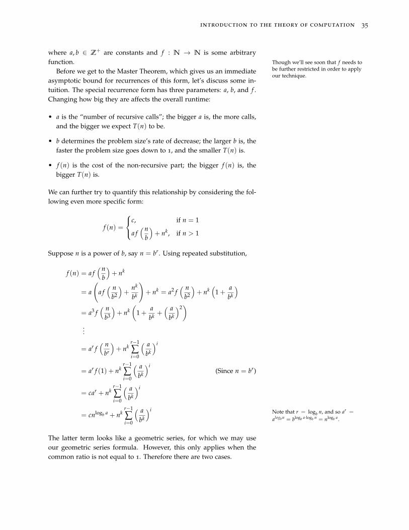
We can further try to quantify this relationship by considering the fol-lowing even more specific form:
f (n) =
c, if n = 1
a f(n
b
)+ nk, if n > 1
Suppose n is a power of b, say n = br. Using repeated substitution,
f (n) = a f(n
b
)+ nk
= a
(a f( n
b2
)+
nk
bk
)+ nk = a2 f
( nb2
)+ nk
(1 +
abk
)= a3 f
( nb3
)+ nk
(1 +
abk +
( abk
)2)
...
= ar f( n
br
)+ nk
r−1
∑i=0
( abk
)i
= ar f (1) + nkr−1
∑i=0
( abk
)i(Since n = br)
= car + nkr−1
∑i=0
( abk
)i
= cnlogb a + nkr−1
∑i=0
( abk
)i
The latter term looks like a geometric series, for which we may use
Note that r = logb n, and so ar =
alogbn = blogb a·logb n = nlogb a.
our geometric series formula. However, this only applies when thecommon ratio is not equal to 1. Therefore there are two cases.
36 david liu
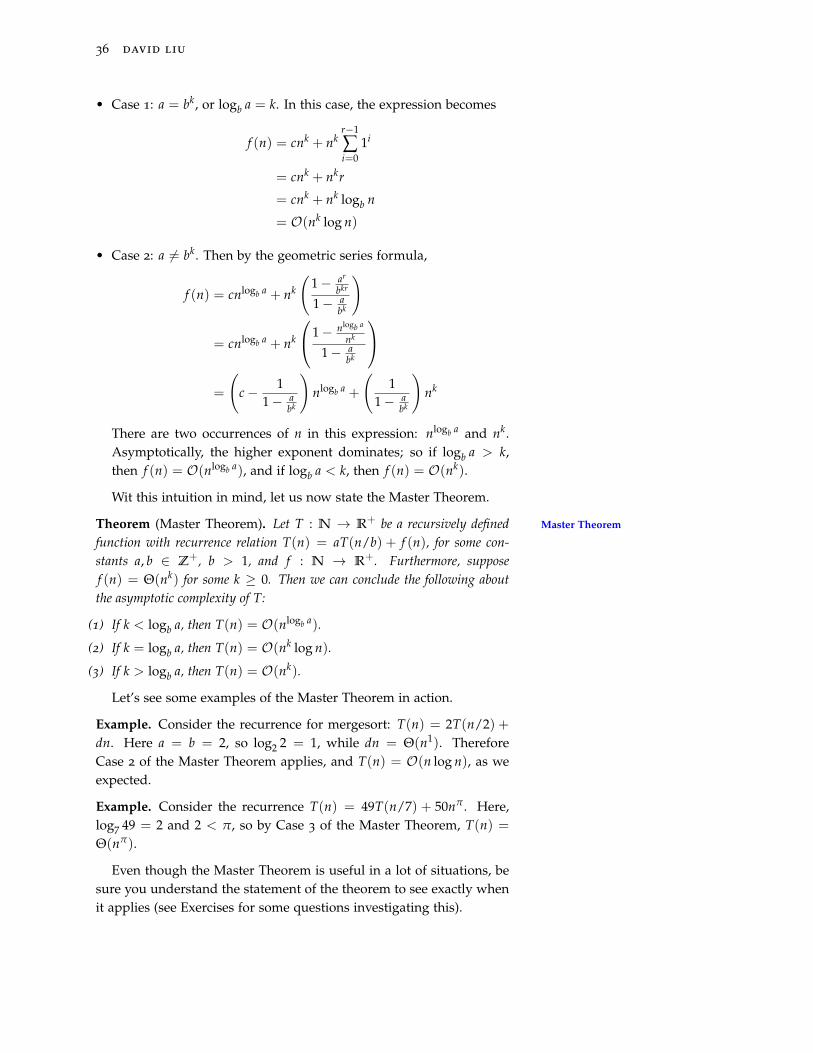
• Case 1: a = bk, or logb a = k. In this case, the expression becomes
f (n) = cnk + nkr−1
∑i=0
1i
= cnk + nkr
= cnk + nk logb n
= O(nk log n)
• Case 2: a 6= bk. Then by the geometric series formula,
f (n) = cnlogb a + nk
(1− ar
bkr
1− abk
)
= cnlogb a + nk
1− nlogb a
nk
1− abk
=
(c− 1
1− abk
)nlogb a +
(1
1− abk
)nk
There are two occurrences of n in this expression: nlogb a and nk.Asymptotically, the higher exponent dominates; so if logb a > k,then f (n) = O(nlogb a), and if logb a < k, then f (n) = O(nk).
Wit this intuition in mind, let us now state the Master Theorem.
Theorem (Master Theorem). Let T : N → R+ be a recursively defined Master Theorem
function with recurrence relation T(n) = aT(n/b) + f (n), for some con-stants a, b ∈ Z+, b > 1, and f : N → R+. Furthermore, supposef (n) = Θ(nk) for some k ≥ 0. Then we can conclude the following aboutthe asymptotic complexity of T:
(1) If k < logb a, then T(n) = O(nlogb a).
(2) If k = logb a, then T(n) = O(nk log n).
(3) If k > logb a, then T(n) = O(nk).
Let’s see some examples of the Master Theorem in action.
Example. Consider the recurrence for mergesort: T(n) = 2T(n/2) +dn. Here a = b = 2, so log2 2 = 1, while dn = Θ(n1). ThereforeCase 2 of the Master Theorem applies, and T(n) = O(n log n), as weexpected.
Example. Consider the recurrence T(n) = 49T(n/7) + 50nπ . Here,log7 49 = 2 and 2 < π, so by Case 3 of the Master Theorem, T(n) =
Θ(nπ).
Even though the Master Theorem is useful in a lot of situations, besure you understand the statement of the theorem to see exactly whenit applies (see Exercises for some questions investigating this).

introduction to the theory of computation 37
Divide-and-Conquer Algorithms
Now that we have seen the Master Theorem, let’s discuss some algo-rithms which we can actually use the Master Theorem to analyse! Akey feature of the recurrence form aT(n/b) + f (n) is that each of therecursive calls has the same size. This naturally leads to the divide-and-conquer paradigm, which can be summarized as follows: divide-and-conquer
An algorithmic paradigm is a generalstrategy for designing algorithms tosolve problems. You will see manymore such strategies in CSC373.
1 divide-and-conquer(P):
2 if P has "small enough" size:
3 return solve_directly(P) # Solve P directly
4 else:
5 divide P into smaller problems P_1, ..., P_k (each of the same size)
6 for i from 1 to k:
7 # Solve each subproblem recursively
8 s_i = divide_and_conquer(P_i)
9 # combine the s_1, ..., s_k to find the correct answer
10 return combine(s_1, ..., s_k)
This is a very general template – in fact, it may seem exactly likeyour mental model of recursion so far, and certainly it is a recursivestrategy. What distinguishes divide-and-conquer algorithms from a lotof other recursive procedures is that we divide the problem into twoor more parts and solve the problems for each part, whereas in general,recursive functions may only make a single recursive call on a singlecomponent of the problem, as in fact or bin_search.
Another common non-divide-and-conquer recursive design patternis taking a list, processing the firstelement, then recursively processingthe rest of the list (and combining theresults).
This introduction to the divide-and-conquer paradigm was delib-erately abstract. However, we have already discussed on divide-and-conquer algorithm: mergesort! Let us now see two classic examples ofdivide-and-conquer algorithms: fast multiplication, and quicksort.
Fast Multiplication
Consider the standard gradeschool algorithm for multiplying two num-bers: 1234× 5678. This requires 16 one-digit multiplications and a fewmore one-digit additions; in general, multiplying two n-digit numbersrequires O(n2) one-digit operations.
Now, let’s see a different way of making this faster. Using a divide-and-conquer approach, we want to split 1234 and 5678 into smallernumbers:
1234 = 12 · 100 + 34, 5678 = 56 · 100 + 78.
Now we use some algebra to write the product 1234 · 5678 as the com-bination of some smaller products: I am not using italics willy-nilly. You
should get used to using these wordwhen talking about divide-and-conqueralgorithms.
1234 · 5678 = (12 · 100 + 34)(56 · 100 + 78)
= (12 · 56) · 10000 + (12 · 78 + 34 · 56) · 100 + 34 · 78
38 david liu
So now instead of multiplying 4-digit numbers, we have shown how tofind the solution by multiplying some 2-digit numbers, a much easierproblem! Note that we aren’t counting multiplication by powers of10, since that amounts to just adding some zeroes to the end of thenumbers.
On a computer, we would use base-2instead of base-10 to take advantageof the “adding zeros,” which corre-sponds to (very fast) bit-shift machineoperations.Reducing 4-digit to 2-digit multiplication may not seem that impres-
sive; but now, we’ll generalize this to arbitrary n-digit numbers (thedifference between multiplying 50-digit vs. 100-digit numbers may bemore impressive).
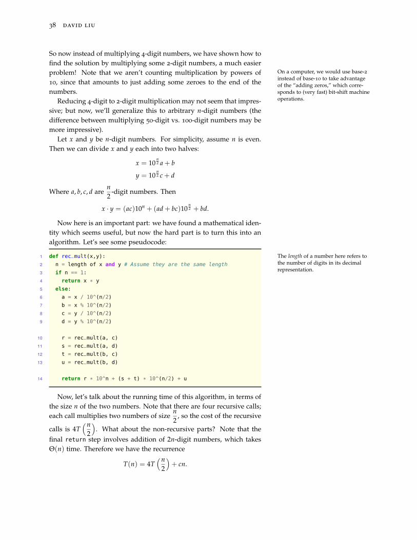
Let x and y be n-digit numbers. For simplicity, assume n is even.Then we can divide x and y each into two halves:
x = 10n2 a + b
y = 10n2 c + d
Where a, b, c, d aren2
-digit numbers. Then
x · y = (ac)10n + (ad + bc)10n2 + bd.
Now here is an important part: we have found a mathematical iden-tity which seems useful, but now the hard part is to turn this into analgorithm. Let’s see some pseudocode:
The length of a number here refers tothe number of digits in its decimalrepresentation.
1 def rec_mult(x,y):
2 n = length of x and y # Assume they are the same length
3 if n == 1:
4 return x * y
5 else:
6 a = x / 10^(n/2)
7 b = x % 10^(n/2)
8 c = y / 10^(n/2)
9 d = y % 10^(n/2)
10 r = rec_mult(a, c)
11 s = rec_mult(a, d)
12 t = rec_mult(b, c)
13 u = rec_mult(b, d)
14 return r * 10^n + (s + t) * 10^(n/2) + u
Now, let’s talk about the running time of this algorithm, in terms ofthe size n of the two numbers. Note that there are four recursive calls;each call multiplies two numbers of size
n2
, so the cost of the recursive
calls is 4T(n
2
). What about the non-recursive parts? Note that the
final return step involves addition of 2n-digit numbers, which takesΘ(n) time. Therefore we have the recurrence
T(n) = 4T(n
2
)+ cn.

introduction to the theory of computation 39
By the Master Theorem, we have T(n) = O(n2).So, this approach didn’t help! We had an arguably more compli-
cated algorithm that achieved the same asymptotic runtime as whatwe learned in elementary school! Moral of the story: Divide-and-conquer, like all algorithmic paradigms, doesn’t always lead to “bet-ter” solutions!
This is a serious lesson. It is not thecase that everything we teach youworks for every situation. It is up touse to use your brain to put togetheryour knowledge to figure out how toapproach problems!
In the case of fast multiplication, though, we can use more mathto improve the running time. Note that the “cross term” ad + bc inthe algorithm required two multiplications to compute naively; how-ever, it is correlated with the values of ac and bd with the followingstraightforward identity:
(a + b)(c + d) = ac + (ad + bc) + bd
(a + b)(c + d)− ac− bd = ad + bc
So we can compute ad + bc by calculating just one additional product(a + b)(c + d) (together with ac and bd).
1 fast_rec_mult(x,y):
2 n = length of x and y (assume they are the same length)
3 if n == 1:
4 return x * y
5 else:
6 a = x / 10^(n/2)
7 b = x % 10^(n/2)
8 c = y / 10^(n/2)
9 d = y % 10^(n/2)
10 p = fast_rec_mult(a + b, c + d)
11 r = fast_rec_mult(a, c)
12 u = fast_rec_mult(b, d)
13 return r * 10^n + (p - r - u) * 10^(n/2) + u
Exercise: what is the runtime of this algorithm now that there areonly three recursive calls?
Quicksort
In this section, we explore the divide-and-conquer sorting algorithmknown as quicksort, which in practice is one of the most commonly quicksort
used. First, we give the pseudocode for this algorithm; note that thisfollows a very clear divide-and-conquer pattern. Unlike fast_rec_multand mergesort, the hard work is done in the divide (partition) step, notthe combine step, which for quicksort is simply list concatenation.
Our naive implementation below doesthis in linear time because of list slicing,but in fact a more clever implementa-tion using indexing accomplishes this inconstant time.

40 david liu
1 def quicksort(A):
2 if len(A) <= 1:
3 do nothing (A is already sorted)
4 else:
5 pick some element x of A (the "pivot")
6 partition (divide) the rest of the elements of A into two lists:
7 - L, the elements of A >= x
8 - G, the elements of A x
9 sort L and G recursively
10 combine the sorted lists in the order L + [x] + G
11 set A equal to the new list
Before moving on, an excellent exercise to try is to take the abovepseudocode and implement quicksort yourself. As we will discussagain and again, implementing algorithms yourself is the best wayto understand them. Remember that the only way to improve yourcoding abilities is to code lots – even something as simple and commonas sorting algorithms offer great practice. See the Exercises for moreexamples.
1 def quicksort(A):
2 if len(A) <= 1:
3 pass
4 else:
5 # Choose the last element as the pivot
6 pivot = A[-1]
7 # Partition the rest of A with respect to the pivot
8 L, G = partition(A[0:-1], pivot)
9 # Sort each list recursively
10 quicksort(L)
11 quicksort(G)
12 # Combine
13 sorted = L + [pivot] + G
14 # Set A equal to the sorted list
15 for i in range(len(A)):
16 A[i] = sorted[i]
17 def partition(A, pivot):
18 L = []
19 G = []
20 for x in A:
21 if x <= pivot:
22 L.append(x)
23 else:
24 G.append(x)
25 return L, G

introduction to the theory of computation 41
Let us try to analyse the running time T(n) of this algorithm, wheren is the length of the input list A. First, the base case n = 1 takesconstant time. The partition method takes linear time, since it iscalled on a list of length n − 1 and contains a for loop which loopsthrough all n − 1 elements. The Python list methods in the rest ofthe code also take linear time, though a more careful implementationcould reduce this. But because partitioning the list always takes lineartime, the non-recursive cost of quicksort is linear.
What about the costs of the recursive steps? There are two of them:quicksort(L) and quicksort(G), so the recursive cost in terms of Land G is T(|L|) and T(|G|). Therefore a potential recurrence is: Here |A| denotes the length of the list
A.
T(n) =
{c, if n ≤ 1
T(|L|) + T(|G|) + dn, if n > 1
What’s the problem with this recurrence? It depends on what L andG are, which in turn depend on the input array and the chosen pivot!In particular, we can’t use either repeated substitution or the MasterTheorem to analyse this function. In fact, the asymptotic running timeof this algorithm can range from Θ(n log n) to Θ(n2) – just as bad asbubblesort! See the Exercises for details.
This begs the question: why is quicksort so used in practice? Tworeasons: quicksort takes Θ(n log n) time “on average”, and careful im- Average-case analysis is slightly more
sophisticated than what we do inthis course, but you can take thisto mean that most of the time, onrandomly selected inputs, quicksorttakes Θ(n log n) time.
plementations of quicksort yield better constants than other Θ(n log n)algorithms, like mergesort. These two facts together imply that quick-sort often outperforms other sorting algorithms in practice!
Exercises
1. Let f : N→N be defined as
f (n) =
{0, if n = 0
f (n− 1) + 2n− 1, if n ≥ 1
Prove using induction that the closed form for f is f (n) = n2.
2. Recall the recursively defined function
f (n) =
0, if n = 1
2, if n = 2
2 f (n− 2), if n > 2
Prove that the closed form for f is
f (n) =
{0, if n is odd
2n2 , if n is even
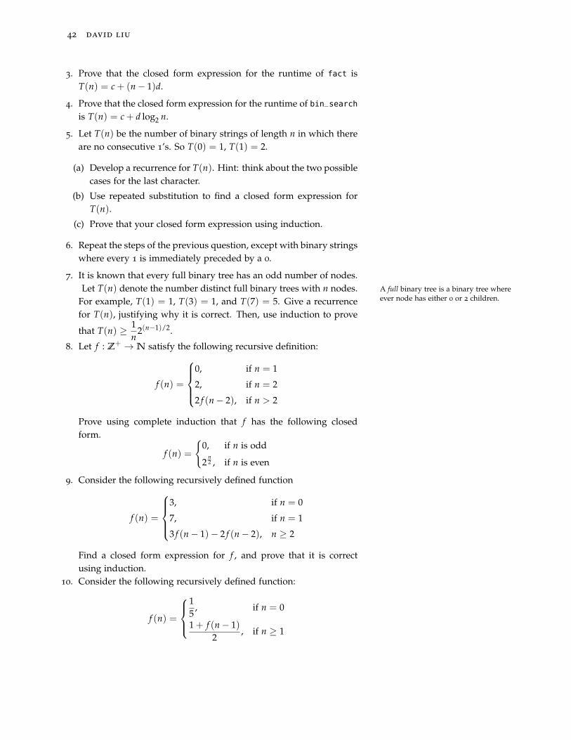
42 david liu
3. Prove that the closed form expression for the runtime of fact isT(n) = c + (n− 1)d.
4. Prove that the closed form expression for the runtime of bin_searchis T(n) = c + d log2 n.
5. Let T(n) be the number of binary strings of length n in which thereare no consecutive 1’s. So T(0) = 1, T(1) = 2.
(a) Develop a recurrence for T(n). Hint: think about the two possiblecases for the last character.
(b) Use repeated substitution to find a closed form expression forT(n).
(c) Prove that your closed form expression using induction.
6. Repeat the steps of the previous question, except with binary stringswhere every 1 is immediately preceded by a 0.
7. It is known that every full binary tree has an odd number of nodes.Let T(n) denote the number distinct full binary trees with n nodes. A full binary tree is a binary tree where
ever node has either 0 or 2 children.For example, T(1) = 1, T(3) = 1, and T(7) = 5. Give a recurrencefor T(n), justifying why it is correct. Then, use induction to prove
that T(n) ≥ 1n
2(n−1)/2.
8. Let f : Z+ →N satisfy the following recursive definition:
f (n) =
0, if n = 1
2, if n = 2
2 f (n− 2), if n > 2
Prove using complete induction that f has the following closedform.
f (n) =
{0, if n is odd
2n2 , if n is even
9. Consider the following recursively defined function
f (n) =
3, if n = 0
7, if n = 1
3 f (n− 1)− 2 f (n− 2), n ≥ 2
Find a closed form expression for f , and prove that it is correctusing induction.
10. Consider the following recursively defined function:
f (n) =
15
, if n = 0
1 + f (n− 1)2
, if n ≥ 1

introduction to the theory of computation 43
(a) Prove that for all n ≥ 1, f (n + 1)− f (n) < f (n)− f (n− 1).
(b) Prove that for all n ∈N, f (n) = 1− 45 · 2n .
11. A block in a binary string is a maximal substring consisting of thesame letter. For example, the string 0100011 has four blocks: 0, 1,000, and 11. Let H(n) denote the number of binary strings of lengthn that have no odd length blocks of 1’s. For example, H(4) = 5:
0000 1100 0110 0011 1111
Develop a recursive definition for H(n), and justify why it is correct.Then find a closed form for H using repeated substitution.
12. Consider the following recursively defined function.
T(n) =
1, if n = 1
4T(n
2
)+ log2 n, otherwise
Use repeated substitution to come up with a closed form expressionfor T(n), when n = 2k; i.e., n is a power of 2. You will need to usethe following identity:
n
∑i=0
i · ai =n · an+2 − (n + 1) · an+1 + a
(a− 1)2 .
13. Analyse the worst-case runtime of fast_rec_mult.14. Analyse the runtime of each of the following recursive algorithms.
It’s up to you to decide whether you should use repeated substitu-tion or the Master Theorem to find the asymptotic bound.
(a)
1 def sum(A):
2 if len(A) == 0:
3 return 1
4 else:
5 return A[0] + sum(A[1..len(A)-1])
(b)
1 def fun(A):
2 if len(A) < 2:
3 return len(A) == 0
4 else:
5 return fun(A[2..len(A)-1])
(c)

44 david liu
1 def double_fun(A):
2 n = len(A)
3 if n < 2:
4 return n
5 else:
6 return double_fun(A[0..n-2]) + double_fun(A[1..n-1])
(d)
1 def mystery(A):
2 if len(A) <= 1:
3 return 1
4 else:
5 d = len(A) // 4 # Integer division
6 s = mystery(A[0..d-1])
7 i = d
8 while i < 3 * d:
9 s += A[i]
10 s += mystery(A[3*d..len(A)-1])
11 return s
15. Recall the recurrence for the worstcase runtime of quicksort fromlecture:
T(n) =
{c, if n ≤ 1
T(|L|) + T(|G|) + dn, if n > 1
where L and G are the partitions of the list. Clearly, how the list ispartitioned matters a great deal for the runtime of quicksort.
(a) Suppose the lists are always evenly split; that is, |L| = |G| = n2
ateach recursive call. Find a tight asymptotic bound on the runtime For simplicity, we’ll ignore the fact that
each list really would have sizen− 1
2.of quicksort using this assumption.
(b) Now suppose that the lists are always very unevenly split: |L| =n− 2 and |G| = 1 at each recursive call. Find a tight asymptoticbound on the runtime of quicksort using this assumption.
Program Correctness
In our study of algorithms so far, we have mainly been concerned withtheir worst-case running time. While this is an important considera-tion of any program, there is arguably a much larger one: programcorrectness! That is, while it is important for our algorithms to runquickly, it is more important that they work! You are used to testingyour programs to demonstrate their correctness, but how confidentyou are in depends on the quality of your testing.
Frankly, developing high quality teststakes a huge amount of time – muchlonger than you probably spent inCSC148!In this chapter, we’ll discuss methods of formally proving program
correctness, without writing any tests at all. We cannot overstate howimportant this technique is: any test suite cannot possibly test a pro-gram on all possible inputs (unless it is a very restricted program), andso this is the only way we can ensure that our programs are actuallycorrect on all inputs. Even for larger software systems, which are fartoo complex to formally prove their correctness, the skills you willlearn in this chapter will enable you to reason more effectively aboutyour code; essentially, what we will teach you is the art of semanticallytracing through code.
By “semantically” we mean yourabililty to derive meaning from code,i.e., identify exactly what the programdoes. This contrasts with programsyntax, things like punctuation andindentation (in Python).
What is Correctness?
You are already familiar with the most common tools used to specifyprogram correctness: preconditions and postconditions. Formally, a pre- precondition/postcondition
condition of a function is a property which an input to the functionmust satisfy in order to guarantee the program will work properly. A As a program designer, it is up to you
to specify preconditions. This often bal-ances the desire of flexibility (allowinga broad range of inputs/usages) withfeasibility (how much code you want orare able to write).
postcondition of a function is a property which must be satisfied afterthe function completes. Most commonly, this refers to properties of areturn value, though it can also refer to changes to the variables passedin, as with the implementation of quicksort from the previous chapter,which didn’t return anything, but instead changed the input list A. A single function can have several pre-
and postconditions.

46 david liu
Example. Consider the following code for calculating the greatest com-mon divisor of two natural numbers. Its pre- and postconditions areshown.
We’ll use mod rather than % in our code,for clarity.
1 def gcd_rec(a, b):
2 ’’’
3 Pre: a and b are positive integers, and a >= b
4 Post: returns the greatest common divisor of a and b
5 ’’’
6 if a == 1 or b == 1:
7 return 1
8 else if a mod b == 0:
9 return b
10 else:
11 return rec_gcd(b, a mod b)
So preconditions tell us what must be true before the programstarts, and postconditions tell us what must be true after the programterminates (assuming it ends at all). We have the following formalstatement of correctness. Though it is written in more formal lan-guage, note that it really captures what we mean when we say that aprogram is “correct.”
Definition (Program Correctness). Let f be a function with a set of program correctness
preconditions and postconditions. Then f is correct (with respect tothe pre- and postconditions) if the following holds:
For every input I to f, if I satisfies the preconditions, thenf(I) terminates, and all the postconditions hold after it ter-minates.
Correctness of Recursive Programs
Consider the code for gcd_rec shown in the previous example. Hereis its statement of correctness:
For all a, b ∈ Z+ such that a ≥ b, rec_gcd(a,b) terminatesand returns gcd(a, b).
How do we prove that gcd_rec is correct? It should come as no sur-prise that we use induction, since you know by now that induction andrecursion are closely related concepts. At this point in the course, youshould be extremely comfortable with the following informal reason-ing: “If a and b are ’small’ then we can prove directly using the basecase of rec_gcd that it is correct. Otherwise, the recursive call happenson ’smaller’ inputs, and by induction, the recursive call is correct, and

introduction to the theory of computation 47
hence because of some {math, logic, etc.}, the program also outputs thecorrect value.”
Writing full induction proofs which formalize the above logic is te-dious, so instead we use the fundamental idea in a looser template. Foreach program path from the first line to a return statement, we showthat it terminates and when it ends, the postconditions are satisfied.We do this by doing the following:
• If the path contains no recursive calls or loops, analyse the code lineby line until the return statement.
• For each recursive call on the path (if there are any), argue why thepreconditions are satisfied at the time of the call, and that the calloccurs on a “smaller” input than the original call. Then you may
There is some ambiguity around whatis meant by “smaller.” We will discussthis shortly.
assume that the postconditions for the recursive call are satisfiedafter the call terminates.
Finally, argue from the last recursive call to the end of the func-tion why the postconditions of the original function call will hold.
• For each loop, use a “loop invariant.” We will deal with this in thenext section.
Pre
Post
Pre
Post
Post
We have described the content of an induction proof; by focusingon tracing values in the code, we are isolating the most importantthinking involved. But recall that the core of induction is proving apredicate for all natural numbers; thus the final ingredient we need toaccount for is associating each input with a natural number: its “size.” So in essence, our “predicate” would be
“for all inputs I of size n that satisfy theprecondition of f, f is correct on I.
Usually, this will be very simple: the length of a list, or the value ofan input number. Let us illustrate this technique using gcd_rec as ourexample.
Example. We will show that gcd_rec is correct. There are three pro-gram paths (this is easy to see, because of the if statements). Let’slook at each one separately.
• Path 1: the program terminates at line 7. If the program goes intothis block, then a = 1 or b = 1. But in these cases, gcd(a, b) = 1,because gcd(1, x) = 1 for all x. Then the postcondition holds, sinceat line 7 the program returns 1.
• Path 2: the program terminates at line 9. If the program goes intothis block, b divides a. Since b is greatest possible divisor of itself,this means that gcd(a, b) = b, and b is returned at line 9.
• Path 3: the program terminates at line 11. We need to check that therecursive call satisfies its preconditions and is called on a smallerinstance. Note that b and (a mod b) are natural numbers, and (amod b) < b, so the preconditions are satisfied. Since a + b > (amod b) + b, the sum of the inputs decreases, and so the recursive callis made on a smaller instance. If you recall the example of using
complete induction on ordered pairs,taking the sum of the two componentswas the size measure we used there,too.
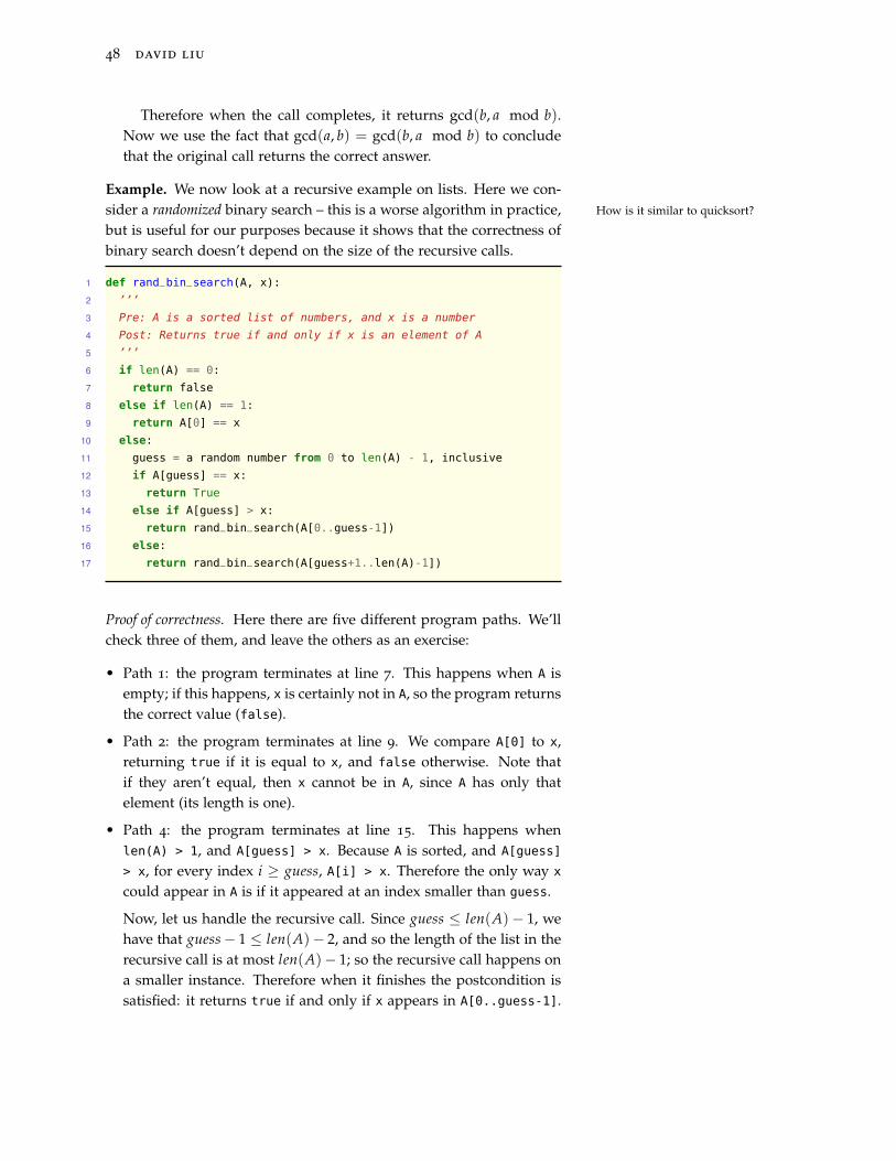
48 david liu
Therefore when the call completes, it returns gcd(b, a mod b).Now we use the fact that gcd(a, b) = gcd(b, a mod b) to concludethat the original call returns the correct answer.
Example. We now look at a recursive example on lists. Here we con-sider a randomized binary search – this is a worse algorithm in practice, How is it similar to quicksort?
but is useful for our purposes because it shows that the correctness ofbinary search doesn’t depend on the size of the recursive calls.
1 def rand_bin_search(A, x):
2 ’’’
3 Pre: A is a sorted list of numbers, and x is a number
4 Post: Returns true if and only if x is an element of A
5 ’’’
6 if len(A) == 0:
7 return false
8 else if len(A) == 1:
9 return A[0] == x
10 else:
11 guess = a random number from 0 to len(A) - 1, inclusive
12 if A[guess] == x:
13 return True
14 else if A[guess] > x:
15 return rand_bin_search(A[0..guess-1])
16 else:
17 return rand_bin_search(A[guess+1..len(A)-1])
Proof of correctness. Here there are five different program paths. We’llcheck three of them, and leave the others as an exercise:
• Path 1: the program terminates at line 7. This happens when A isempty; if this happens, x is certainly not in A, so the program returnsthe correct value (false).
• Path 2: the program terminates at line 9. We compare A[0] to x,returning true if it is equal to x, and false otherwise. Note thatif they aren’t equal, then x cannot be in A, since A has only thatelement (its length is one).
• Path 4: the program terminates at line 15. This happens whenlen(A) > 1, and A[guess] > x. Because A is sorted, and A[guess]
> x, for every index i ≥ guess, A[i] > x. Therefore the only way x
could appear in A is if it appeared at an index smaller than guess.
Now, let us handle the recursive call. Since guess ≤ len(A)− 1, wehave that guess− 1 ≤ len(A)− 2, and so the length of the list in therecursive call is at most len(A)− 1; so the recursive call happens ona smaller instance. Therefore when it finishes the postcondition issatisfied: it returns true if and only if x appears in A[0..guess-1].
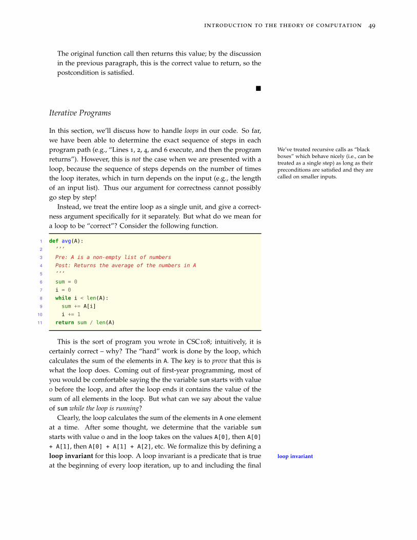
introduction to the theory of computation 49
The original function call then returns this value; by the discussionin the previous paragraph, this is the correct value to return, so thepostcondition is satisfied.
�
Iterative Programs
In this section, we’ll discuss how to handle loops in our code. So far,we have been able to determine the exact sequence of steps in eachprogram path (e.g., “Lines 1, 2, 4, and 6 execute, and then the programreturns”). However, this is not the case when we are presented with a
We’ve treated recursive calls as “blackboxes” which behave nicely (i.e., can betreated as a single step) as long as theirpreconditions are satisfied and they arecalled on smaller inputs.
loop, because the sequence of steps depends on the number of timesthe loop iterates, which in turn depends on the input (e.g., the lengthof an input list). Thus our argument for correctness cannot possiblygo step by step!
Instead, we treat the entire loop as a single unit, and give a correct-ness argument specifically for it separately. But what do we mean fora loop to be “correct”? Consider the following function.
1 def avg(A):
2 ’’’
3 Pre: A is a non-empty list of numbers
4 Post: Returns the average of the numbers in A
5 ’’’
6 sum = 0
7 i = 0
8 while i < len(A):
9 sum += A[i]
10 i += 1
11 return sum / len(A)
This is the sort of program you wrote in CSC108; intuitively, it iscertainly correct – why? The “hard” work is done by the loop, whichcalculates the sum of the elements in A. The key is to prove that this iswhat the loop does. Coming out of first-year programming, most ofyou would be comfortable saying the the variable sum starts with value0 before the loop, and after the loop ends it contains the value of thesum of all elements in the loop. But what can we say about the valueof sum while the loop is running?
Clearly, the loop calculates the sum of the elements in A one elementat a time. After some thought, we determine that the variable sum
starts with value 0 and in the loop takes on the values A[0], then A[0]
+ A[1], then A[0] + A[1] + A[2], etc. We formalize this by defining aloop invariant for this loop. A loop invariant is a predicate that is true loop invariant
at the beginning of every loop iteration, up to and including the final

50 david liu
loop iteration. Usually, the predicate will depend on which iterationthe loop is on, or more generally, the value(s) of the program variable(s)associated with the loop. For example, in avg, the loop invariant corre-sponding to our previous intuition is
By convention, the empty sum−1
∑k=0
A[k]
evaluates to 0.
P(i, sum) : sum =i−1
∑k=0
A[k]
The i and sum in the predicate really correspond to the values of thosevariables in the code for avg. That is, this predicate is stating a propertyof these variables in the code.
Unfortunately, this loop invariant isn’t quite right; what if i >
len(A)? Then the sum is not well-defined, since, for example, A[len(A)]is undefined. This can be solved with a common technique for loopinvariants: putting bounds on “loop counter” variables, as follows:
Inv(i, sum) : 0 ≤ i ≤ len(A) ∧ sum =i−1
∑k=0
A[k].
This ensures that the sum is always well-defined, and has the addedbenefit of explicitly defining a possible range of values on i.
In general, the fewer possible values avariable takes on, the fewer cases youhave to worry about in your code.
A loop invariant is correct if it is always true at the beginning ofevery loop iteration, including the loop check which fails, causing the loopto terminate. This is why we allowed i ≤ len(A) rather than just i <len(A) in the invariant.
How do we prove that loop invariants are correct? The argument isyet another application of induction:
• First, we argue that the loop invariant is satisfied when the loop isreached. (This is arrow (1) in the diagram)
• Then, we argue that if the loop invariant is satisfied at the beginningof an iteration, then after the loop body executes once (i.e., one loopiteration occurs), the loop invariant still holds. (Arrow (2))
• Finally, after proving that the loop invariant is correct, we show thatif the invariant holds when the loop ends, then the postconditionwill be satisfied when the program returns. (Arrow (3))
Pre
Inv
Post
(1)
(2)
(3)
Though this is basically an inductive proof, as was the case for recur-sive programs, we won’t hold to the formal induction structure here. If we wanted to be precise, we would
do induction on the number of loopiterations executed.
Example. Let us formally prove that avg is correct. The main portionof the proof will be the proof that our loop invariant P(i) is correct.
Proof. When the program first reaches the loop, i = 0 and sum = 0.Plugging this into the predicate yields
Inv(0, 0) : 0 ≤ 0 ≤ len(A) ∧ 0 =−1
∑k=0
A[k],

introduction to the theory of computation 51
which is true (recall the note about the empty sum from earlier).Now suppose the loop iteration holds when i = i0, at the beginning
of a loop iteration. Let sum0 be the value of the variable sum at thistime. The loop invariant we are assuming is the following:
Inv(i0, sum0) : 0 ≤ i0 ≤ len(A) ∧ sum0 =i0−1
∑k=0
A[k].
What happens next? The obvious answer is “the loop body runs,” butthis misses one subtle point: if i0 = len(A) (which is allowed by theloop invariant), the body of the loop doesn’t run, and we don’t need toworry about this case, since we only care about checking what happensto the invariant when the loop actually runs.
So assume that i0 < len(A), so that the loop body runs. Whathappens in one iteration? Two things: sum increases by A[i0], and i
increases by 1. Let sum1 and i1 be the values of sum and i at the end ofthe loop iteration. We have sum1 = sum0 + A[i0] and i1 = i0 + 1. Ourgoal is to prove that the loop invariant holds for i1 and sum1, i.e.,
Inv(i1, sum1) : 0 ≤ i1 ≤ len(A) ∧ sum1 =i1−1
∑k=0
A[k].
Let us check that the loop invariant is still satisfied by sum1 and i1.First, 0 ≤ i0 < i1 = i0 + 1 ≤ len(A), where the first inequality camefrom the loop invariant holding at the beginning of the loop, and thelast inequality came from the assumption that i0 < len(A). The secondpart of Inv can be checked by a simple calculation:
sum1 = sum0 + A[i0]
=
(i0−1
∑k=0
A[k]
)+ A[i0] (by Inv(i0, sum0))
=i0
∑k=0
A[k]
=i1−1
∑k=0
A[k] (Since i1 = i0 + 1)
Therefore the loop invariant always holds.The next key idea is that when the loop ends, variable i has value
len(A), since by the loop invariant it always has value ≤ len(A), andif it were strictly less than len(A), another iteration of the loop would
run. Then by the loop invariant, the value of sum islen(A)−1
∑k=0
A[k], i.e.,
the sum of all the elements in A! The last step is to continue tracingIt might seem like a lot of writing to getto what we said paragraphs ago, butthis is a formal argument that confirmsour intuition.until the program returns, which in this case takes just a single step:

52 david liu
the program returns sum / len(A). But this is exactly the average ofthe numbers in A, because the variable sum is equal their sum!
We also implicitly use here the mathe-matical definition of “average” as thesum of the numbers divided by howmany there are.Therefore the postcondition is satisfied. �
Note the deep connection between the loop invariant and the post-condition. There are many other loop invariants we could have chosen:for example, Inv(i, sum) : i + sum ≥ 0. But this wouldn’t have helpedat all in proving the postcondition! When confronting more problemson your own, it will be up to you to determine the right loop invariantsfor the job; keep in mind that choosing loop invariants can usually bedone by either by taking a high-level approach and mimicking some-thing in the postcondition, or, a low-level approach by tracing throughthe code slowly on test inputs to try to find patterns in the variablevalues.
One final warning before we move on: loop invariants describe rela-tionships between variables at a specific moment in time. Students often Specifically, at the beginning of a
particular loop check.try to use loop invariants to capture how variables change over time (e.g.,“i will increase by 1 when the loop runs”), which creates massiveheadaches because determining how the code works is the meat ofa proof, and shouldn’t be shoehorned into a single predicate! Whenworking with more complex code, we take the view that loop invari-ants are properties that are preserved, even if they don’t describe ex-actly how the code works or exactly what happens! This flexibility iswhat makes correctness proofs manageable.
Example. Here we consider a numerical example: a low level imple-mentation of multiplication.
1 def mult(a,b):
2 ’’’
3 Pre: a and b are natural numbers
4 Post: returns a * b
5 ’’’
6 m = 0
7 count = 0
8 while count < b:
9 m += a
10 count += 1
11 return m
Proof of correctness. The key thing to figure out here is how the loopworks. It’s clear what it’s supposed to do: the variable m changes from0 at the beginning of the loop to a*b at the end. How does this changehappen? One simple thing we could do is make a table of values ofthe variables m and count as the loop progresses:
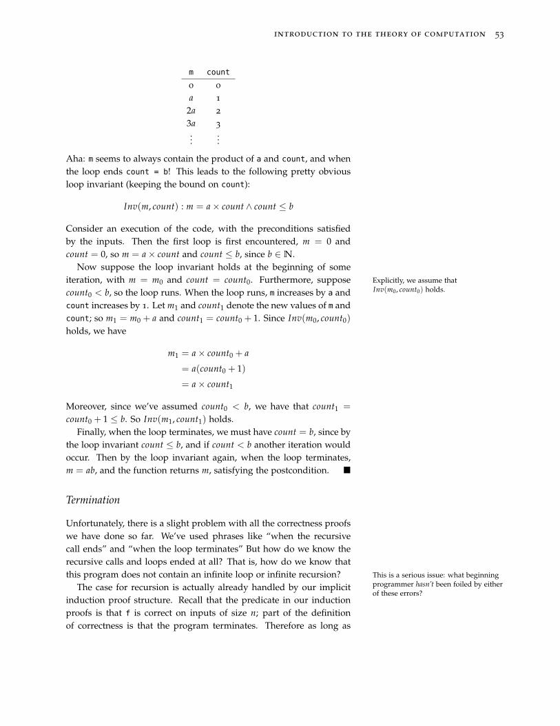
introduction to the theory of computation 53
m count
0 0
a 1
2a 2
3a 3
......
Aha: m seems to always contain the product of a and count, and whenthe loop ends count = b! This leads to the following pretty obviousloop invariant (keeping the bound on count):
Inv(m, count) : m = a× count ∧ count ≤ b
Consider an execution of the code, with the preconditions satisfiedby the inputs. Then the first loop is first encountered, m = 0 andcount = 0, so m = a× count and count ≤ b, since b ∈N.
Now suppose the loop invariant holds at the beginning of someiteration, with m = m0 and count = count0. Furthermore, suppose Explicitly, we assume that
Inv(m0, count0) holds.count0 < b, so the loop runs. When the loop runs, m increases by a andcount increases by 1. Let m1 and count1 denote the new values of m andcount; so m1 = m0 + a and count1 = count0 + 1. Since Inv(m0, count0)
holds, we have
m1 = a× count0 + a
= a(count0 + 1)
= a× count1
Moreover, since we’ve assumed count0 < b, we have that count1 =
count0 + 1 ≤ b. So Inv(m1, count1) holds.Finally, when the loop terminates, we must have count = b, since by
the loop invariant count ≤ b, and if count < b another iteration wouldoccur. Then by the loop invariant again, when the loop terminates,m = ab, and the function returns m, satisfying the postcondition. �
Termination
Unfortunately, there is a slight problem with all the correctness proofswe have done so far. We’ve used phrases like “when the recursivecall ends” and “when the loop terminates” But how do we know therecursive calls and loops ended at all? That is, how do we know thatthis program does not contain an infinite loop or infinite recursion? This is a serious issue: what beginning
programmer hasn’t been foiled by eitherof these errors?
The case for recursion is actually already handled by our implicitinduction proof structure. Recall that the predicate in our inductionproofs is that f is correct on inputs of size n; part of the definitionof correctness is that the program terminates. Therefore as long as

54 david liu
the induction structure holds – i.e., that the recursive calls are gettingsmaller and smaller – termination comes for free.
The case is a little trickier for loops. As an example, consider theloop in avg. Because the loop invariant Inv(i, sum) doesn’t say any-thing about how i changes, we can’t use it to prove that the loopterminates. But for most loops, including this one, it is “obvious” whythey terminate, because they typically have counter variables which it-erate through a fixed range of values.
This role is played by the variablei, which goes through the range{0, 1, . . . , len(A)− 1}.
This argument would certainly convince us that this loop termi-nates, and in general all loops with this form of loop counter termi-nate. However, not all loops you will see or write in your life will havesuch an obvious loop counter. Here’s an example:
1 def collatz(n):
2 ’’’ Pre: n is a natural number ’’’
3 curr = n
4 while curr > 1:
5 if curr is even:
6 curr = curr / 2
7 else:
8 curr = 3 * curr + 1
In fact, it is an open question in math-ematics whether this function haltson all inputs or not. If only we had acomputer program that could tell uswhether it does!
Therefore we’ll now introduce a formal way of proving loop termi-nation. Recall from the recursive case that our proofs hinged on the loop termination
fact that the recursive calls were made on smaller and smaller inputs,until some base case was reached. Our strategy for loops will drawinspiration from this: we associate with the loop a loop measure m loop measure
which has the following two properties:
(1) m decreases with each iteration of the loop
(2) m is always a natural number at the beginning of each loop iteration
While this is not the only strategy forproving termination, it turns out tobe suitable for most loops involvingnumbers and lists. When you studymore advanced data structures andalgorithms, you will discuss morecomplex arguments for both correctnessand termination.
If such an m exists, then at some point m won’t be able to decrease anyfurther (because 0 is the smallest natural number), and therefore theloop cannot have any more iterations. This is analogous to inputs torecursive calls getting smaller and smaller until a base case is reached.
Let us illustrate this technique on our avg loop.
Example. Proof of termination of avg. Even though we’ve already ob-served that the loop has a natural loop counter variable i, this variableincreases with each iteration. Instead, our loop measure variable willbe m = len(A)− i. Let us check that m satisfies the properties (1) and(2):
(1) Since at each iteration i increases by 1, and len(A) stays the same,m = len(A)− i decreases by 1 each iteration.
(2) Note that i and len(A) are both always natural numbers. But thisalone is not enough to conclude that m ∈N; for example, 3, 5 ∈N

introduction to the theory of computation 55
but (3− 5) /∈ N. But the loop invariant we proved included thepredicate 0 ≤ i ≤ len(A), and because of this we can conclude thatlen(A)− i ≥ 0, so len(A)− i ∈N.
This is a major reason we includesuch loop counter bounds on the loopinvariant.
Since we have established that m is a decreasing loop measure for theloop, this loop terminates, and therefore avg terminates (since everyother line of code is a simple step which certainly terminates). �
Notice that the above termination proof relied on i increasing by 1
each step, and never exceeding len(A). That is, we basically just usedthe fact that i was a standard loop counter. Here is a more complexexample where there is no obvious loop counter.
Example. Prove that the following function terminates:
1 def term_ex(x,y):
2 ’’’ Pre: x and y are natural numbers. ’’’
3 a = x
4 b = y
5 while a > 0 or b > 0:
6 if a > 0:
7 a -= 1
8 else:
9 b -= 1
10 return x * y
Proof. Intuitively, the loop terminates because when the loop runs, ei-ther a or b decreases, and will stop when a and b reach 0. To makethis argument formal, we need the following loop invariant: a, b ≥ 0,whose proof we leave as an exercise.
The loop measure we define is m = a + b. Let us prove the necessaryproperties for m:
• In the loop, either a decreases by 1, or b decreases by 1. In eithercase, m = a + b decreases by 1. Therefore m is decreasing.
• Since our loop invariant says that a, b ≥ 0, we have that m ≥ 0 aswell. Therefore m ∈N. �
Exercises
1. Here is some code which recursively determines the smallest ele-ment of a list. Give pre- and postconditions for this function, thenprove it is correct according to your specifications.
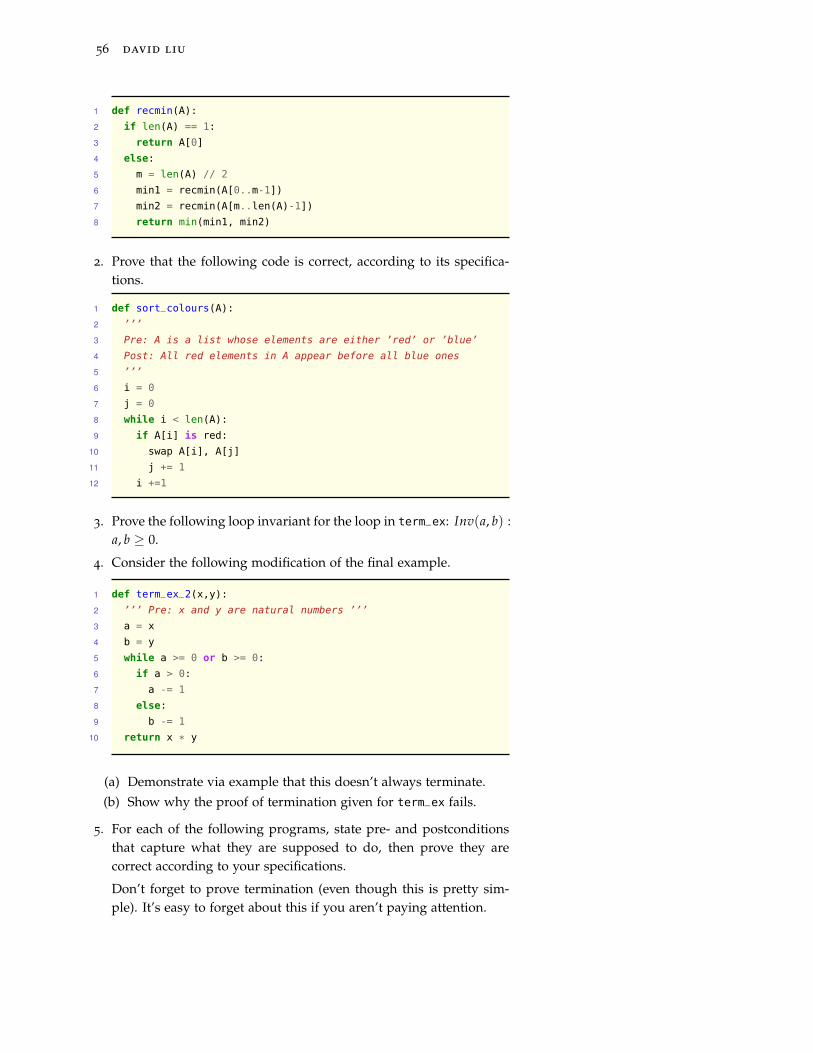
56 david liu
1 def recmin(A):
2 if len(A) == 1:
3 return A[0]
4 else:
5 m = len(A) // 2
6 min1 = recmin(A[0..m-1])
7 min2 = recmin(A[m..len(A)-1])
8 return min(min1, min2)
2. Prove that the following code is correct, according to its specifica-tions.
1 def sort_colours(A):
2 ’’’
3 Pre: A is a list whose elements are either ’red’ or ’blue’
4 Post: All red elements in A appear before all blue ones
5 ’’’
6 i = 0
7 j = 0
8 while i < len(A):
9 if A[i] is red:
10 swap A[i], A[j]
11 j += 1
12 i +=1
3. Prove the following loop invariant for the loop in term_ex: Inv(a, b) :a, b ≥ 0.
4. Consider the following modification of the final example.
1 def term_ex_2(x,y):
2 ’’’ Pre: x and y are natural numbers ’’’
3 a = x
4 b = y
5 while a >= 0 or b >= 0:
6 if a > 0:
7 a -= 1
8 else:
9 b -= 1
10 return x * y
(a) Demonstrate via example that this doesn’t always terminate.(b) Show why the proof of termination given for term_ex fails.
5. For each of the following programs, state pre- and postconditionsthat capture what they are supposed to do, then prove they arecorrect according to your specifications.
Don’t forget to prove termination (even though this is pretty sim-ple). It’s easy to forget about this if you aren’t paying attention.
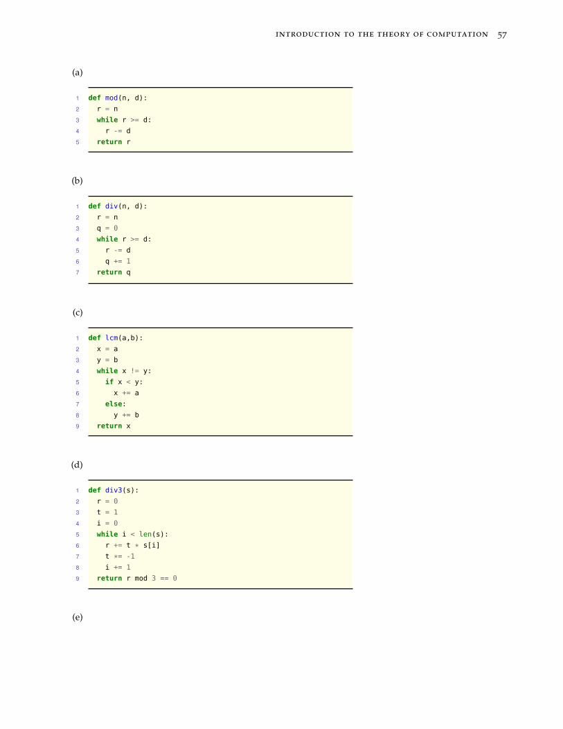
introduction to the theory of computation 57
(a)
1 def mod(n, d):
2 r = n
3 while r >= d:
4 r -= d
5 return r
(b)
1 def div(n, d):
2 r = n
3 q = 0
4 while r >= d:
5 r -= d
6 q += 1
7 return q
(c)
1 def lcm(a,b):
2 x = a
3 y = b
4 while x != y:
5 if x < y:
6 x += a
7 else:
8 y += b
9 return x
(d)
1 def div3(s):
2 r = 0
3 t = 1
4 i = 0
5 while i < len(s):
6 r += t * s[i]
7 t *= -1
8 i += 1
9 return r mod 3 == 0
(e)
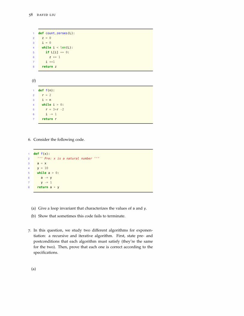
58 david liu
1 def count_zeroes(L):
2 z = 0
3 i = 0
4 while i < len(L):
5 if L[i] == 0:
6 z += 1
7 i +=1
8 return z
(f)
1 def f(n):
2 r = 2
3 i = n
4 while i > 0:
5 r = 3*r -2
6 i -= 1
7 return r
6. Consider the following code.
1 def f(x):
2 ’’’ Pre: x is a natural number ’’’
3 a = x
4 y = 10
5 while a > 0:
6 a -= y
7 y -= 1
8 return a * y
(a) Give a loop invariant that characterizes the values of a and y.
(b) Show that sometimes this code fails to terminate.
7. In this question, we study two different algorithms for exponen-tiation: a recursive and iterative algorithm. First, state pre- andpostconditions that each algorithm must satisfy (they’re the samefor the two). Then, prove that each one is correct according to thespecifications.
(a)

introduction to the theory of computation 59
1 def exp_rec(a, b):
2 if b == 0:
3 return 1
4 else if b mod 2 == 0:
5 x = exp_rec(a, b / 2)
6 return x * x
7 else:
8 x = exp_rec(a, (b - 1)/2)
9 return x * x * a
(b)
1 def exp_iter(a, b):
2 ans = 1
3 mult = 0
4 exp = b
5 while exp > 0:
6 if exp mod 2 == 1:
7 ans *= mult
8 mult *= a
9 exp = floor(exp / 2)
10 return ans
8. Prove that the following function is correct. Warning: this one isprobably the most difficult to prove correct. But, it runs in lineartime – pretty amazing!
1 def majority(A):
2 ’’’
3 Pre: A is a list with more than half its entries equal to x
4 Post: Returns the majority element x
5 ’’’
6 c = 1
7 m = 0
8 i = 1
9 while i <= len(A) - 1:
10 if c == 0:
11 m = A[i]
12 c == 1
13 else if A[i] == m:
14 c += 1
15 else:
16 c -= 1
17 i += 1
18 return m
9. Here we study yet another sorting algorithm, bubblesort.

60 david liu
1 def bubblesort(L):
2 ’’’
3 Pre: L is a list of numbers
4 Post: L is sorted
5 ’’’
6 k = 0
7 while k < len(L):
8 i = 0:
9 while i < len(L) - k:
10 if L[i] > L[i+1]:
11 swap L[i] and L[i+1]
12 i += 1
13 k +=1
(a) State and prove an invariant for the inner loop.
(b) State and prove an invariant for the outer loop.
(c) Prove that bubblesort is correct, according to its specifications.
10. Consider the following generalization of the min function.
1 def extract(L, k):
2 ’’’
3 Pre: L is a list of distinct numbers, k is a positive integer
4 Post: Returns the k-th smallest element of L
5 ’’’
6 count = 1
7 index = 0
8 try = 1
9 while count < k:
10 if L[index] < L[try]:
11 index = try
12 count += 1
13 try +=1
14 swap L[index], L[len(L) - 1]
15 last = L[len(L) - 1]
16 A = [last]
17 i = 0
18 while i < len(L) - 1:
19 if L[i] <= last:
20 A.append(L[i])
21 i += 1
22 return extract(A, k)
(a) State and prove a loop invariant for first loop.
(b) State and prove a loop invariant for second loop.
(c) Using your loop invariants, prove that the program is correct.

introduction to the theory of computation 61
(d) Prove that the following recursive program accomplishes the sametask.
1 def extract(A, k):
2 pivot = A[0]
3 # Use partition from quicksort
4 L, G = partition(A[1..len(A) - 1], pivot)
5 if len(L) == k - 1:
6 return pivot
7 else if len(L) >= k:
8 return extract(L, k)
9 else:
10 return extract(G, k - len(L) - 1)


Regular Languages & Finite Automata
In this final chapter, we turn our attention to the study of finite au-tomata, a simple model of computation with surprisingly deep ap-plications ranging from vending machines to neurological systems.We focus on one particular application: matching regular languages,which are the foundation of natural language processing, includingtext searching and parsing. This application alone makes automataan invaluable computational tool, one with which you are probablyalready familiar in the guise of regular expressions.
Definitions
We open with some definitions related to strings. An alphabet Σ is a fi- alphabet
nite set of symbols, e.g., {0, 1}, {a, b, . . . , z}, or {0, 1, . . . , 9,+,−,×,÷}.A string over an alphabet Σ is a finite sequence of symbols from Σ. string
Therefore “0110” is a string over {0, 1}, and “abba” and “cdbaaaa” arestrings over {a, b, c, d}. The empty string “”, denoted by ε, consists of a Σ: Greek letter “Sigma”, ε: “epsilon”
sequence of zero symbols from the alphabet. We use the notation Σ∗
to denote the set of all strings over the alphabet Σ.The length of a string w ∈ Σ∗ is the number of symbols appearing length
in the string, and is denoted |w|. For example, |ε| = 0, |aab| = 3,and |11101010101| = 11. We use Σn to denote the set of strings overΣ of length n. For example, if Σ = {0, 1}, then Σ0 = {ε} and Σ2 =
{00, 01, 10, 11}. So Σ∗ = Σ0 ∪ Σ1 ∪ Σ2 ∪ · · ·A language over an alphabet Σ is a subset of strings L ⊆ Σ∗. Unlike language
The “English language” is a subset ofthe words which can be formed by allpossible combinations of the usual 26
letters.
alphabets and strings, languages may be either finite or infinite. Hereare some examples of languages over the alphabet {a, b, c}:
{ε, a, b, ccc}{w ∈ {a, b, c}∗ | |w| ≤ 3}{w ∈ {a, b, c}∗ | w has the same number of a’s and c’s}{w ∈ {a, b, c}∗ | w can be found in an English dictionary}
These are pretty mundane examples. Somewhat surprisingly, how-ever, this notion of languages also captures solutions to computational

64 david liu
problems. Consider the following languages over the alphabet of allstandard ASCII characters.
E.g., “[1, 2, 76]′′ ∈ L1
L1 = {A | A is a string representation of a sorted list of numbers}L2 = {(A, x) | A is a list of numbers, x is the minimum of A}L3 = {(a, b, c) | a, b, c ∈N and gcd(a, b) = c}L4 = {(P, x) | P is a Python program that halts when given input x}
So we can interpret many computer programs as deciding membership ina particular language. For example, a program which decides whetheran input string is in L1 is essentially a program that decides whetheran input list is sorted.
Students of CSC165 will recall thatmembership in L4 cannot be computedby any program at all – this is thefamous Halting Problem!Solutions to computational problems are just one face of the coin;
what about the programs we create to solve them? One of the greatachievements of the early computer scientist Alan Turing was the de-velopment of the Turing Machine, an abstract model of computationthat is just as powerful as the physical computers we use today. Unfor-tunately, Turing Machines are a far more powerful and complex modelthan is appropriate for this course. Instead, we will study the simpler You will study Turing Machines to your
heart’s content in CSC463.computational model of finite automata, and the class of languages theycompute: regular languages.
Regular Languages
Regular languages are the most basic kind of languages, and are de-rived from rather simple language operations. In particular, we definethe following three operations for languages L, M ⊆ Σ∗:
• Union: The union of L and M is the language L ∪M = {x ∈ Σ∗ | union
x ∈ L or x ∈ M}.• Concatenation: The concatenation of L and M is the language LM = concatenation
{xy ∈ Σ∗ | x ∈ L, y ∈ M}.• Kleene Star: The (Kleene) star of L is language L∗ = {ε} ∪ {x ∈ Σ∗ | Kleene star
∃w1, w2, . . . , wn ∈ L such that x = w1w2 . . . wn, for some n}. Thatis, L∗ contains the words which can be broken down into 0 or moresmaller words, each of which is in L.
The star operation can be thought ofin terms of union and concatenation asL∗ = {ε} ∪ L ∪ LL ∪ LLL ∪ · · ·
Example. Consider the languages L = {a, bb} and M = {a, c}. Thenwe have
L ∪M = {a, bb, c}LM = {aa, ac, bba, bbc}
L∗ = {ε, a, aa, bb, aaa, abb, bba, . . . }M∗ = {ε, a, c, aa, ac, ca, cc, aaa, aac, . . . }
Note that M∗ = {a, c}∗ is exactly thewords which are made up of only a’sand c’s. This explains the notation Σ∗
to denote the set of all strings over thealphabet Σ.
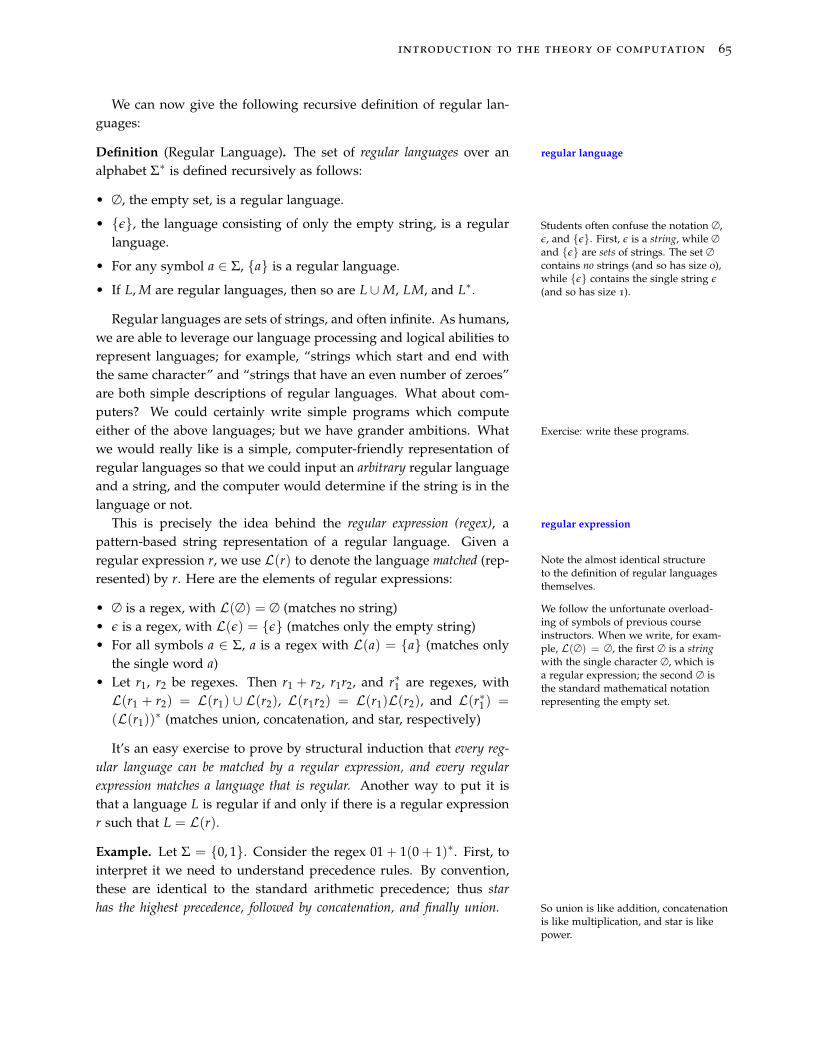
introduction to the theory of computation 65
We can now give the following recursive definition of regular lan-guages:
Definition (Regular Language). The set of regular languages over an regular language
alphabet Σ∗ is defined recursively as follows:
• ∅, the empty set, is a regular language.
• {ε}, the language consisting of only the empty string, is a regularlanguage.
• For any symbol a ∈ Σ, {a} is a regular language.
• If L, M are regular languages, then so are L ∪M, LM, and L∗.
Students often confuse the notation ∅,ε, and {ε}. First, ε is a string, while ∅and {ε} are sets of strings. The set ∅contains no strings (and so has size 0),while {ε} contains the single string ε(and so has size 1).
Regular languages are sets of strings, and often infinite. As humans,we are able to leverage our language processing and logical abilities torepresent languages; for example, “strings which start and end withthe same character” and “strings that have an even number of zeroes”are both simple descriptions of regular languages. What about com-puters? We could certainly write simple programs which computeeither of the above languages; but we have grander ambitions. What Exercise: write these programs.
we would really like is a simple, computer-friendly representation ofregular languages so that we could input an arbitrary regular languageand a string, and the computer would determine if the string is in thelanguage or not.
This is precisely the idea behind the regular expression (regex), a regular expression
pattern-based string representation of a regular language. Given aregular expression r, we use L(r) to denote the language matched (rep-resented) by r. Here are the elements of regular expressions:
Note the almost identical structureto the definition of regular languagesthemselves.
• ∅ is a regex, with L(∅) = ∅ (matches no string) We follow the unfortunate overload-ing of symbols of previous courseinstructors. When we write, for exam-ple, L(∅) = ∅, the first ∅ is a stringwith the single character ∅, which isa regular expression; the second ∅ isthe standard mathematical notationrepresenting the empty set.
• ε is a regex, with L(ε) = {ε} (matches only the empty string)• For all symbols a ∈ Σ, a is a regex with L(a) = {a} (matches only
the single word a)• Let r1, r2 be regexes. Then r1 + r2, r1r2, and r∗1 are regexes, withL(r1 + r2) = L(r1) ∪ L(r2), L(r1r2) = L(r1)L(r2), and L(r∗1) =
(L(r1))∗ (matches union, concatenation, and star, respectively)
It’s an easy exercise to prove by structural induction that every reg-ular language can be matched by a regular expression, and every regularexpression matches a language that is regular. Another way to put it isthat a language L is regular if and only if there is a regular expressionr such that L = L(r).
Example. Let Σ = {0, 1}. Consider the regex 01 + 1(0 + 1)∗. First, tointerpret it we need to understand precedence rules. By convention,these are identical to the standard arithmetic precedence; thus starhas the highest precedence, followed by concatenation, and finally union. So union is like addition, concatenation
is like multiplication, and star is likepower.
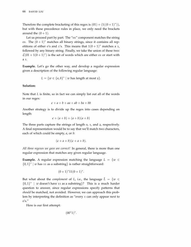
66 david liu
Therefore the complete bracketing of this regex is (01) + (1((0+ 1)∗)),but with these precedence rules in place, we only need the bracketsaround the (0 + 1).
Let us proceed part by part. The “01” component matches the string01. The (0 + 1)∗ matches all binary strings, since it contains all rep-etitions of either 0’s and 1’s. This means that 1(0 + 1)∗ matches a 1,followed by any binary string. Finally, we take the union of these two:L(01 + 1(0 + 1)∗) is the set of words which are either 01 or start witha 1.
Example. Let’s go the other way, and develop a regular expressiongiven a description of the following regular language:
L = {w ∈ {a, b}∗ | w has length at most 2}.
Solution:
Note that L is finite, so in fact we can simply list out all of the wordsin our regex:
ε + a + b + aa + ab + ba + bb
Another strategy is to divide up the regex into cases depending onlength:
ε + (a + b) + (a + b)(a + b)
The three parts capture the strings of length 0, 1, and 2, respectively.A final representation would be to say that we’ll match two characters,each of which could be empty, a, or b:
(ε + a + b)(ε + a + b).
All three regexes we gave are correct! In general, there is more than oneregular expression that matches any given regular language.
Example. A regular expression matching the language L = {w ∈{0, 1}∗ | w has 11 as a substring} is rather straightforward:
(0 + 1)∗11(0 + 1)∗.
But what about the complement of L, i.e., the language L̄ = {w ∈{0, 1}∗ | w doesn’t have 11 as a substring}? This is a much harderquestion to answer, since regular expressions specify patterns thatshould be matched, not avoided. However, we can approach this prob-lem by interpreting the definition as “every 1 can only appear next to0’s.”
Here is our first attempt:
(00∗1)∗.

introduction to the theory of computation 67
Inside the brackets, 00∗1 matches a non-empty block of 0’s followedby a 1, and this certainly ensures that there are no consecutive 1’s. Un-fortunately, this regular expression matches only a subset of L, and notL entirely. For example, the string 1001 is in L, but can’t be matchedby this regular expression because the first 1 isn’t preceded by any 0’s.We can fix this by saying that the first character could possibly be a 1:
(ε + 1)(00∗1)∗.
There is one last problem: this fails to match any string that ends with0’s, e.g., 0100. We can apply a similar fix as the previous one to allowa block of 0’s to be matched at the end:
(ε + 1)(00∗1)∗0∗.
Some interesting meta-remarks arise naturally from the last exam-ple. One is a rather straightforward way of showing that a languageand regex are inequivalent, by simply producing a word that is in onebut not the other. On the other hand, convincing ourselves that a regu-
Keep this is mind when you andyour friends are arguing about whoseregular expressions are correct.
lar expression correctly matches a language can be quite difficult; howdid we know that (ε + 1)(00∗1)∗0∗ correctly matches L? Proving thata regex matches a particular language L is much harder, because weneed to show that every string in L is matched by the regex, and everystring not in L is not.
Note that this is a universally quantifiedstatement, while its negation (regexdoesn’t match L) is existentially quan-tified. This explains the difference indifficulty.
Our intuition only takes us so far – it is precisely this gap betweenour gut and true understanding that proofs were created to fill. This is,however, just a little beyond the scope of the course; you have all thenecessary ingredients – surprise: induction – but the arguments for allbut the simplest languages are quite involved. We will see later that reasoning about
the correctness of deterministic finiteautomata is just as powerful, and a littlesimpler.
Example. We finish off this section with a few corner cases to illus-trate some of the subtleties in our definition, and extend the arithmeticmetaphor we hinted at earlier. First, the following equalities show that∅ plays the role of the “zero” in regular expressions. Let r be an arbi-trary regular expression.
By equality between regular expressionswe mean that they match the samelanguage. That is, r1 = r2 ⇔ L(r1) =L(r2).
∅ + r = r + ∅ = r
∅r = r∅ = ∅
The first is obvious because taking the union of any set with the emptyset doesn’t change the set. What about concatenation? Recall that con-catenation of languages involves taking combinations of words fromthe first language and words from the second; if one of the two lan-guages is empty, then no combinations are possible.
We can use similar arguments to show that ε plays the role of the

68 david liu
“one”:
εr = rε = r
ε∗ = ε
A Suggestive Flowchart
You might be wondering how computers actually match strings to reg-ular expressions. It turns out that regular languages are rather easy tomatch because of the following (non-obvious!) property:
You can determine membership in a regular language byreading letters of the string one at a time, left to right.
q0 q1
0
1
1
0
Consider the flowchart-type object shown in the figure on the right.Suppose we start at the state marked q0. Now consider the string 0110,reading the letters one at a time, left to right, and following the arrowsmarked by the letters we read in. It is not hard to see that we end upat state q0. On the other hand, if the string is 111, we end up at stateq1. The state q1 is marked as special by a double-border; we say that astring ending up at q1 is accepted, while a string ending at q0 is rejected.
After some thought you may realise that the accepted strings areexactly the ones with an odd number of 1’s. A more suggestive wayof saying this is that the language accepted by this flowchart is the set ofstrings with an odd number of 1’s.
Deterministic Finite Automata
We now use the notion of “flowcharts” to define a simple model ofcomputation. Each one acts as a simple computer program: starting ata particular point, it receives inputs from the user, updates its internalmemory, and when the inputs are over, it outputs True or False. Thefollowing definition is likely one of the most technical you’ve encoun-tered to date, in this course and others. Make sure you fully under-stand the prior example, and try to match it to the formal definition asyou read it.
Definition (Deterministic Finite Automaton). A deterministic finiteautomaton (DFA) (denoted D) is a quintuple D = (Q, Σ, δ, s, F) where deterministic finite automaton
the components define the various parts of the automaton:
• Q is the (finite) set of states in D
• Σ is the alphabet of symbols used by D
• δ : Q× Σ→ Q is the transition function (represents the “arrows”)
• s ∈ Q is the initial state of D

introduction to the theory of computation 69
• F ⊆ Q is the set of accepting (final) states of D
Example. In the introductory example, the state set is Q = {q0, q1},the alphabet is {0, 1}, the initial state is q0, and the set of final states is{q1}. We can represent the transition function as a table of values:
Note that there’s only one final state inthis example, but in general there maybe several final states.
Old State Letter New Stateq0 0 q0
q0 1 q1
q1 0 q1
q1 1 q0
In general, the number of “rows” in the transition function table is|Q| · |Σ|; each state must have exactly |Σ| transitions leading out of it,each labelled with a unique symbol in Σ.
Before proceeding, make sure you understand each of the followingstatements about how DFAs work:
• DFAs read strings one letter at a time, from left to right
• DFAs cannot “go back” and reread previous letters
• At a particular state, once you have read a letter there is only onearrow (transition) you can follow
• DFAs have a finite amount of memory, since they have a finite num-ber of states
• Inputs to DFAs can be any length
• Because of these last two points, it is impossible for DFAs to alwaysremember every letter they have read so far
A quick note about notation before proceeding with a few moreexamples. Technically, δ takes as its second argument a letter; e.g.,δ(q0, 1) = q1 (from the previous example). But we can just as easilyextend this definition to arbitrary length words in the second argu-ment. For example, we can say δ(q0, 11) = q0, δ(q1, 1000111) = q1, andδ(q0, ε) = q0. For every state q, δ(q, ε) = q.
With this “extended” transition function, it is very easy to symboli-cally represent the language L(D) accepted by the DFA D. Recall that the language accepted by a
DFA is the set of strings accepted by it.
L(D) = {w ∈ Σ∗ | δ(s, w) ∈ F}
Example. Let us design a DFA that accepts the following language:
L = {w ∈ {a, b}∗ | w starts with a and ends with b}.
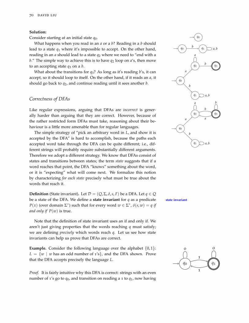
70 david liu
Solution:Consider starting at an initial state q0. q0
q0 q1b
a, b
q0
q1
q2 q3
b
a
a, b
a
b
q0
q1
q2 q3
b
a
a, b
a
b
a
b
What happens when you read in an a or a b? Reading in a b shouldlead to a state q1 where it’s impossible to accept. On the other hand,reading in an a should lead to a state q2 where we need to “end with ab.” The simple way to achieve this is to have q2 loop on a’s, then moveto an accepting state q3 on a b.
What about the transitions for q3? As long as it’s reading b’s, it canaccept, so it should loop to itself. On the other hand, if it reads an a, itshould go back to q2, and continue reading until it sees another b.
Correctness of DFAs
Like regular expressions, arguing that DFAs are incorrect is gener-ally harder than arguing that they are correct. However, because ofthe rather restricted form DFAs must take, reasoning about their be-haviour is a little more amenable than for regular languages.
The simple strategy of “pick an arbitrary word in L, and show it isaccepted by the DFA” is hard to accomplish, because the paths eachaccepted word take through the DFA can be quite different; i.e., dif-ferent strings will probably require substantially different arguments.Therefore we adopt a different strategy. We know that DFAs consist ofstates and transitions between states; the term state suggests that if aword reaches that point, the DFA “knows” something about the word,or it is “expecting” what will come next. We formalize this notionby characterizing for each state precisely what must be true about thewords that reach it.
Definition (State invariant). Let D = (Q, Σ, δ, s, F) be a DFA. Let q ∈ Qbe a state of the DFA. We define a state invariant for q as a predicate state invariant
P(x) (over domain Σ∗) such that for every word w ∈ Σ∗, δ(s, w) = q ifand only if P(w) is true.
Note that the definition of state invariant uses an if and only if. Wearen’t just giving properties that the words reaching q must satisfy;we are defining precisely which words reach q. Let us see how stateinvariants can help us prove that DFAs are correct.
Example. Consider the following language over the alphabet {0, 1}:L = {w | w has an odd number of 1’s}, and the DFA shown. Provethat the DFA accepts precisely the language L.
q0 q1
0
1
1
0
Proof. It is fairly intuitive why this DFA is correct: strings with an evennumber of 1’s go to q0, and transition on reading a 1 to q1, now having

introduction to the theory of computation 71
an odd number of 1’s. Here are some state invariants for the two states:
δ(q0, w) = q0 ⇔ w has an even number of 1’s
δ(q0, w) = q1 ⇔ w has an odd number of 1’s
Here are two important properties to keep in mind when designingstate invariants:
• The state invariants should be mutually exclusive. That is, thereshould be no overlap between them; no string should satisfy twodifferent state invariants. Otherwise, to which state would the stringgo?
• The state invariants should be exhaustive. That is, they should coverall possible cases; every string in Σ∗, including ε, should satisfy oneof the state invariants. Otherwise, the string goes nowhere.
These conditions are definitely satisfied by our two invariants above,since every string has either an even or odd number of 1’s.
Next, we want to prove that the state invariants are correct. We dothis in two steps.
• Show that the empty string ε satisfies the state invariant of theinitial state. In our case, the initial state is q0; ε has zero 1’s, whichis even; therefore the state invariant is satisfied by ε.
• For each transition q a−→ r, show that if a word w satisfies theinvariant of state q, then the string wa satisfies the invariant ofr. (That is, each transition respects the invariants.) There are four The astute reader will note that we are
basically doing a proof by inductionon the length of the strings. Like ourproofs of program correctness, we“hide” the formalities of inductionproofs and focus only on the content.
transitions in our DFA. For the two 0-loops, appending a 0 to astring doesn’t change the number of 1’s in the string, and hence ifw contains an even (odd) number of 1’s, then w0 contains an even(odd) number of 1’s as well, so these two transitions are correct.
On the other hand, appending a 1 increases the number of 1’s ina string by one. So if w contains an even (odd) number of 1’s, w1contains an odd (even) number of 1’s, so the transitions between q0
to q1 labelled 1 preserve the invariants.
Thus we have proved that the state invariants are correct. The finalstep is to show that the state invariants at the accepting state(s) pre-cisely describe the target language. This is very obvious in this case, Remember that in general, there can be
more than one accepting state!because the only accepting state is q1, and its state invariant is exactlythe defining characteristic of the target language L. �
Limitations of DFAs
Not only does the simplicity of the DFA model enable proofs of cor-rectness; we can also determine inherent limitations of the model. In

72 david liu
this section, we’ll cover two examples. First, we prove a lower boundon the number of states required in a DFA accepting a particular lan-guage. Then, we’ll show that certain languages cannot be accepted byDFAs of any size!
Example. Consider the language
L = {w ∈ {0, 1}∗ | w has at least three 1’s.}.
We’ll prove that any DFA accepting this language has at least 4 states.
Proof. Suppose there exists a DFA D = (Q, Σ, δ, s, F) that accepts L andhas fewer than four states. Consider the four strings w0 = ε, w1 = 1,w2 = 11, and w3 = 111. By the Pigeonhole Principle, two of these wordsreach the same state in D from the initial state. Let’s give these objectsnames: suppose 0 ≤ i < j ≤ 3, and δ(s, wi) = δ(s, wj) = q for somestate q ∈ Q.
The Pigeonhole Principle states that ifm > n, and you are putting m pigeonsinto n holes, then two pigeons will gointo the same hole.
Now, since wi and wj reach the same state, they are indistinguishableprefixes to the DFA; this means that any words of the form wix and wjxwill end up at the same state in the DFA, and hence are both acceptedor both rejected. However, suppose x = w3−j. Then wix = w3−j+i andwjx = w3. Then wix contains 3− j + i 1’s, and wjx contains three 1’s.But since i < j, 3− j + i < 3, so wix /∈ L, while wjx ∈ L. Therefore wixand wjx cannot end up at the same state in D, a contradiction! �
The key idea in the above proof was that the four different wordsε, 1, 11, 111 all had to reach different states, because there were suffixesthat could distinguish any pair of them. In general, to prove that a These were the x = w3−j in the proof.
language L requires at least k states in a DFA to accept it, it sufficesto gives a set of k strings, each of which is distinguishable from theothers with respect to L. In case it isn’t clear, two strings w1 and
w2 are “distinguishable with respectto L” if there is a suffix x such thatw1x ∈ L and w2x /∈ L, or vice versa.
Now we turn to a harder problem: proving that some languagescannot be accepted by DFAs of any size.
Example. Consider the language L = {0n1n | n ∈ N}. Prove that noDFA accepts L.
Proof. We’ll prove this by contradiction again. Suppose there is a DFAD = (Q, Σ, δ, s, F) that accepts L. Let k = |Q|, the number of statesin D. Now here is the key idea: D has only k states of “memory,”whereas to accept L, you really have to remember the exact numberof 0’s you’ve read in so far, so that you can match that number of 1’slater. So we should be able to “overload” the memory of D.
Here’s how: consider the string w = 0k+1, i.e., the string consistingof k + 1 0’s. Since there are only k states in D, the path that w takesthrough D must involve a loop starting at some state q. That is, we
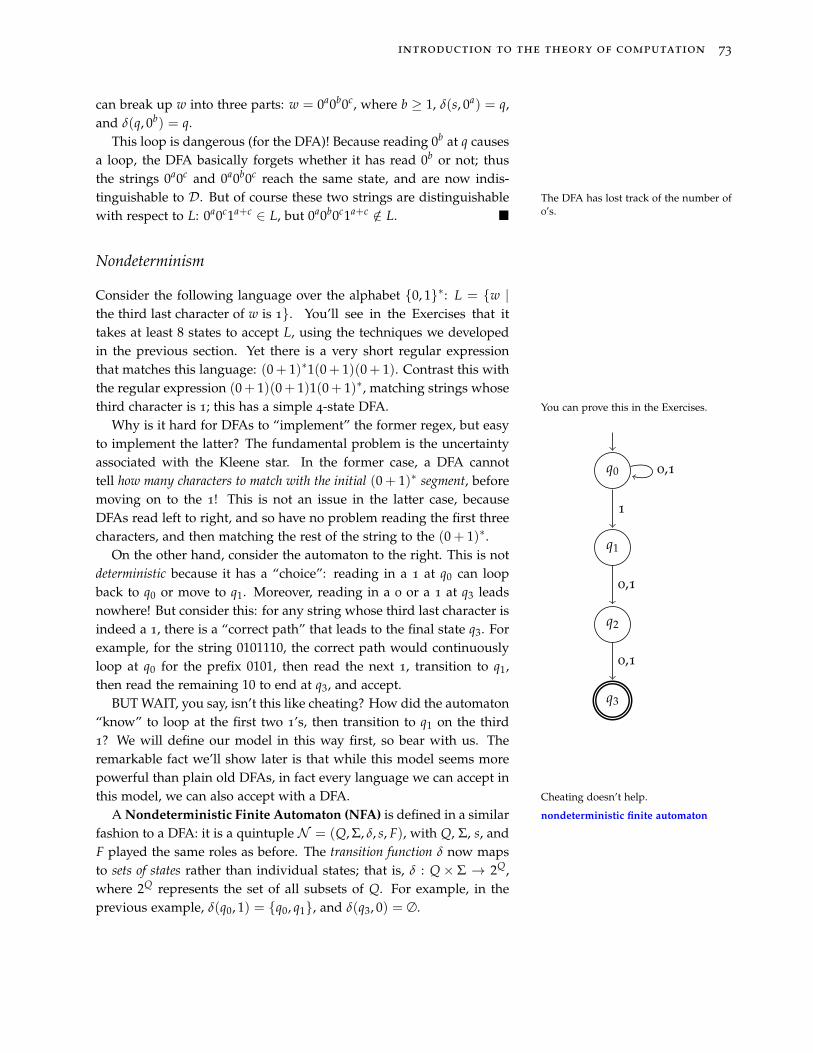
introduction to the theory of computation 73
can break up w into three parts: w = 0a0b0c, where b ≥ 1, δ(s, 0a) = q,and δ(q, 0b) = q.
This loop is dangerous (for the DFA)! Because reading 0b at q causesa loop, the DFA basically forgets whether it has read 0b or not; thusthe strings 0a0c and 0a0b0c reach the same state, and are now indis-tinguishable to D. But of course these two strings are distinguishable The DFA has lost track of the number of
0’s.with respect to L: 0a0c1a+c ∈ L, but 0a0b0c1a+c /∈ L. �
Nondeterminism
Consider the following language over the alphabet {0, 1}∗: L = {w |the third last character of w is 1}. You’ll see in the Exercises that ittakes at least 8 states to accept L, using the techniques we developedin the previous section. Yet there is a very short regular expressionthat matches this language: (0+ 1)∗1(0+ 1)(0+ 1). Contrast this withthe regular expression (0+ 1)(0+ 1)1(0+ 1)∗, matching strings whosethird character is 1; this has a simple 4-state DFA. You can prove this in the Exercises.
Why is it hard for DFAs to “implement” the former regex, but easyto implement the latter? The fundamental problem is the uncertaintyassociated with the Kleene star. In the former case, a DFA cannottell how many characters to match with the initial (0 + 1)∗ segment, beforemoving on to the 1! This is not an issue in the latter case, becauseDFAs read left to right, and so have no problem reading the first threecharacters, and then matching the rest of the string to the (0 + 1)∗.
q0
q1
q2
q3
0,1
1
0,1
0,1
On the other hand, consider the automaton to the right. This is notdeterministic because it has a “choice”: reading in a 1 at q0 can loopback to q0 or move to q1. Moreover, reading in a 0 or a 1 at q3 leadsnowhere! But consider this: for any string whose third last character isindeed a 1, there is a “correct path” that leads to the final state q3. Forexample, for the string 0101110, the correct path would continuouslyloop at q0 for the prefix 0101, then read the next 1, transition to q1,then read the remaining 10 to end at q3, and accept.
BUT WAIT, you say, isn’t this like cheating? How did the automaton“know” to loop at the first two 1’s, then transition to q1 on the third1? We will define our model in this way first, so bear with us. Theremarkable fact we’ll show later is that while this model seems morepowerful than plain old DFAs, in fact every language we can accept inthis model, we can also accept with a DFA. Cheating doesn’t help.
A Nondeterministic Finite Automaton (NFA) is defined in a similar nondeterministic finite automaton
fashion to a DFA: it is a quintuple N = (Q, Σ, δ, s, F), with Q, Σ, s, andF played the same roles as before. The transition function δ now mapsto sets of states rather than individual states; that is, δ : Q× Σ → 2Q,where 2Q represents the set of all subsets of Q. For example, in theprevious example, δ(q0, 1) = {q0, q1}, and δ(q3, 0) = ∅.

74 david liu
We think of δ(q, a) here as representing the set of possible states reach-able from q by reading in the letter a. This is extended in the naturalway to δ(q, w) for arbitrary length strings w to mean all states reach-able from q by reading in the word w. Note that if a path reaches astate q and next symbol a with δ(q, a) = ∅, then this path “aborts,”i.e., the NFA does not continue reading more characters for this path.
We say that a word w is accepted by NFA N if δ(s, w) ∩ F 6= ∅; thatis, if there exists a final state reachable from the initial state by readingthe word w. Note that the existential quantifier used in the definitionof acceptance is an integral part of the definition: we don’t require thatevery path leading out of s along w reach a final state, only one. Thisformalizes the notion that it be possible to choose the correct path, evenfrom among many rejecting or aborted paths.
On the other hand, if a string is rejectedby an NFA, this means all possiblepaths that string could take eitheraborted or ended at a rejecting state.
ε-transitions
We can augment NFAs even further through the use of ε-transitions. ε-transition
These are nondeterministic transitions which do not require readingin a letter to activate. That is, if you are currently at state q on anNFA, and there is an ε-transition from q to another state r, then youcan transition to r without reading the next letter in the word.
q rε
For instance, the NFA on the right accepts the string 0 by takingthe ε-transition to q1, reading the 0 to reach q2, then taking anotherε-transition to q3. q0
q1
q2
q3
q4
q5
εε
0
ε, 0
1
As was the case for nondeterminism, ε-transitions do not actuallyadd any power to the model, although they can be useful in certainconstructions that we’ll use in the next section.
Equivalence of Definitions
So far in this chapter, we have used both DFAs and regular expressionsto represent the class of regular languages. We have taken for grantedthat DFAs are sufficient to represent regular languages; in this section,we will prove this formally. There is also the question of nondeter-minism: do NFAs accept a larger class of languages than DFAs? Inthis section, we’ll show that the answer, somewhat surprisingly, is no.Specifically, we will sketch a proof of this theorem.
Theorem (Equivalence of Representations of Regular Languages). LetL be a language over an alphabet Σ. Then the following are equivalent:
(1) There is a regular expression that matches L.
(2) There is a deterministic finite automaton that accepts L.
(3) There is a nondeterministic finite automaton (possibly with ε-transitions)that accepts L.
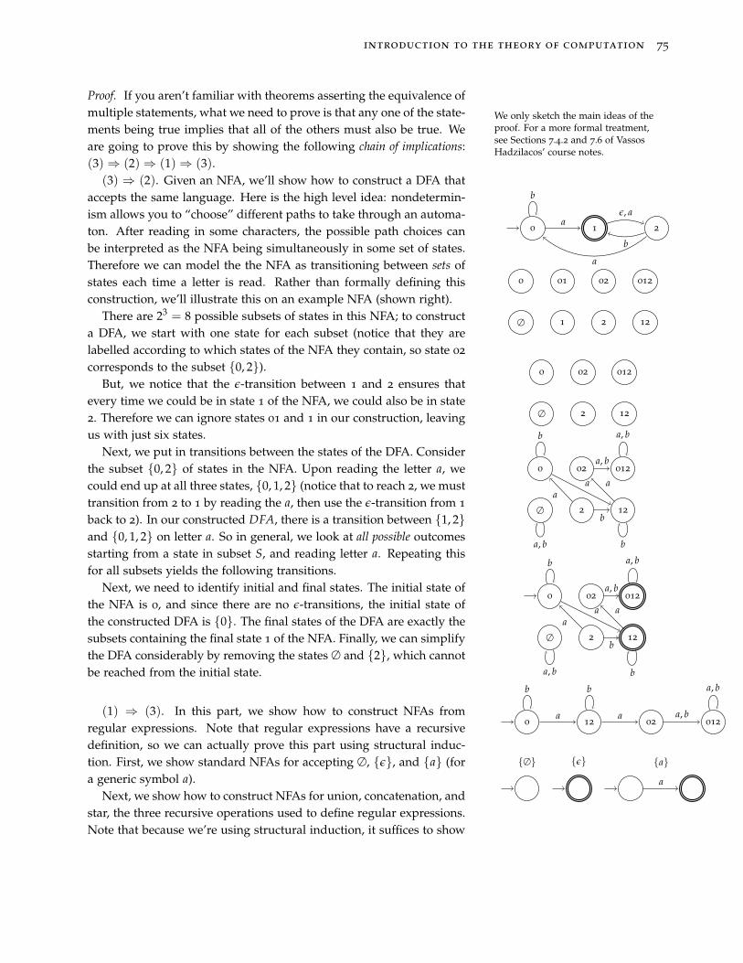
introduction to the theory of computation 75
Proof. If you aren’t familiar with theorems asserting the equivalence ofmultiple statements, what we need to prove is that any one of the state-ments being true implies that all of the others must also be true. Weare going to prove this by showing the following chain of implications:(3)⇒ (2)⇒ (1)⇒ (3).
We only sketch the main ideas of theproof. For a more formal treatment,see Sections 7.4.2 and 7.6 of VassosHadzilacos’ course notes.
(3) ⇒ (2). Given an NFA, we’ll show how to construct a DFA thataccepts the same language. Here is the high level idea: nondetermin-ism allows you to “choose” different paths to take through an automa-ton. After reading in some characters, the possible path choices canbe interpreted as the NFA being simultaneously in some set of states.Therefore we can model the the NFA as transitioning between sets ofstates each time a letter is read. Rather than formally defining thisconstruction, we’ll illustrate this on an example NFA (shown right).
0 1 2
b
aε, a
b
a
There are 23 = 8 possible subsets of states in this NFA; to constructa DFA, we start with one state for each subset (notice that they arelabelled according to which states of the NFA they contain, so state 02
corresponds to the subset {0, 2}).
0 01 02 012
∅ 1 2 12
0 02 012
∅ 2 12
0 02 012
∅ 2 12
b
a
a, b
a, b
a, b
a
b
a
b
0 02 012
∅ 2 12
b
a
a, b
a, b
a, b
a
b
a
b
0 12 02 012
b
a a, b
a, b
a
b
But, we notice that the ε-transition between 1 and 2 ensures thatevery time we could be in state 1 of the NFA, we could also be in state2. Therefore we can ignore states 01 and 1 in our construction, leavingus with just six states.
Next, we put in transitions between the states of the DFA. Considerthe subset {0, 2} of states in the NFA. Upon reading the letter a, wecould end up at all three states, {0, 1, 2} (notice that to reach 2, we musttransition from 2 to 1 by reading the a, then use the ε-transition from 1
back to 2). In our constructed DFA, there is a transition between {1, 2}and {0, 1, 2} on letter a. So in general, we look at all possible outcomesstarting from a state in subset S, and reading letter a. Repeating thisfor all subsets yields the following transitions.
Next, we need to identify initial and final states. The initial state ofthe NFA is 0, and since there are no ε-transitions, the initial state ofthe constructed DFA is {0}. The final states of the DFA are exactly thesubsets containing the final state 1 of the NFA. Finally, we can simplifythe DFA considerably by removing the states ∅ and {2}, which cannotbe reached from the initial state.
(1) ⇒ (3). In this part, we show how to construct NFAs fromregular expressions. Note that regular expressions have a recursivedefinition, so we can actually prove this part using structural induc-tion. First, we show standard NFAs for accepting ∅, {ε}, and {a} (fora generic symbol a).
{∅} {ε}
a
{a}
Next, we show how to construct NFAs for union, concatenation, andstar, the three recursive operations used to define regular expressions.Note that because we’re using structural induction, it suffices to show

76 david liu
how to perform these operations on NFAs; that is, given two NFAsN1 and N2, construct NFAs accepting L(N1) ∪ L(N2), L(N1)L(N2),and (L(N1))
∗. We use the notation on the right to denote genericNFAs; the two accepting states on the right side of each box symbolizeall accepting states of the NFAs, and their starts states are s1 and s2,respectively.
s1
N1
s2
N2
First consider union. This can be accepted by the NFA shown tothe right. Essentially, the idea is that starting a new new initial state,we “guess” whether the word will be accepted by N1 or N2 by ε-transitioning to either s1 or s2, and then see if the word is actuallyaccepted by running the corresponding NFA. s
s1
N1
s2
N2
ε
εFor concatenation, we start with the first NFA N1, and then every
time we reach a final state, we “guess” that the matched string fromL(N1) is complete, and ε-transition to the start state of N2.
s1
N1
s2
N2
ε
ε
Finally, for the Kleene star we perform a similar construction, exceptthe final states ofN1 ε-transition to s1 rather than s2. To possibly acceptε, we add a new initial state that is also accepting.
s s1
N1
ε
ε
ε
(2) ⇒ (1). Finally, we show how to construct regular expressionsfrom DFAs. This is the hardest construction to prove, so our sketchhere will be especially vague. The key idea is the following:
For any two states q, r in a DFA, there is a regular expressionthat matches precisely the words w such that δ(q, w) = r;i.e., the words that induce a path from q to r.
Let D = (Q, Σ, δ, s, F) be a DFA with n states, Q = {1, . . . , n}. Foreach i, j ∈ Q, we define the sets Lij = {w | δ(i, w) = j}; our ultimategoal is to show that every Lij can be matched by a regular expression.To do this, we use a clever induction argument. For every 0 ≤ k ≤ n, This part was first proved by Sephen
Kleene, the inventor of regular expres-sions and after whom the Kleene star isnamed.
let
Lij(k) = {w | δ(i, w) = j, and only states ≤ k are passed between i and j}
Note that Lij(0) is the set of words where there must be no interme-diate states, i.e., w is a letter labelling a transition directly from i to j.Also, Lij(n) = Lij: no restrictions are placed on the states that can bepassed. We will show how to inductively build up regular expressionsmatching each of the Lij(k), where the induction is done on k. First,the base case, which we’ve already described intuitively:
Formally, our predicate is P(k) : “Forall states i and j, the set Lij(k) can bematched by a regex.”
Lij(0) =
{{a ∈ Σ | δ(i, a) = j}, if i 6= j
{a ∈ Σ | δ(i, a) = j} ∪ {ε}, if i = j
Note that when i = j, we need to include ε, as this indicates the trivialact of following no transition at all. Since the Lij(0) are finite sets (ofsymbols), we can write regular expressions for them (e.g., if Lij(0) =
{a, c, f }, the regex would be a + c + f ).You can prove this fact in the Exercises.

introduction to the theory of computation 77
Finally, here is the recursive definition of the sets that will allow usto construct regular languages: it defines Lij(k + 1) in terms of someL...(k), using only the operations of union, concatenation, and star:
Lij(k + 1) = Lij(k) ∪(
Li,k+1(k)Lk+1,k+1(k)∗Lk+1,j(k))
Therefore given regular expressions for Lij(k), Li,k+1(k), Lk+1,k+1(k),and Lk+1,j(k), we can construct a regular expression for Lij(k + 1).
�
Exercises
1. For each of the following regular languages over the alphabet Σ =
{0, 1}, design a regular expression and DFA which accepts that lan-guage. For which languages can you design an NFA that is substan-tially smaller than your DFA?
(a) {w | w contains an odd number of 1’s}(b) {w | w contains exactly two 1’s}(c) {w | w contains 011}(d) {w | w ends with 00}(e) {w | |s| is a multiple of 3}(f) {w | every 0 in w is eventually followed by a 1}(g) {w | w does not begin with 10}(h) {w | w is the binary representation of a multiple of three}(i) {w | w contains both 00 and 11 as substrings}(j) {0n1m | m, n ∈N, m + n is even}
(k) {w | w contains a substring of length at most 5 that has at least three 1’s}(l) {w | w has an even number of zeroes, or exactly 2 ones}
2. Let L = {w ∈ {0, 1}∗ | the third last character of w is a 1}. Provethat every DFA accepting L has at least 8 states. Hint: Consider the8 binary strings of length 3. For a bonus, what is the smallest DFA
you can find that accepts L? It shouldhave more than 8 states!
3. Prove by induction that every finite language can be representedby a regular expression. (This shows that all finite languages areregular.)
4. Prove that the following languages are not regular.
(a) {an2 | n ∈N}(b) {xx | x ∈ 0, 1∗}(c) {w ∈ {a, b}∗ | w has more 0’s than 1’s}(d) {w ∈ {0, 1}∗ | w has two blocks of 0’s with the same length}(e) {anbmcn−m | n ≥≥ 0}

78 david liu
5. Recall that the complement of a language L ⊆ Σ∗ is the set L =
{w ∈ Σ∗ | w /∈ L}.
(a) Given a DFA D = (Q, Σ, δ, s, F) which accepts a language L, de-scribe how you can construct a DFA that accepts L.
(b) Let L be a language over an alphabet Σ. Prove that if L is notregular, then the complement of L is not regular.
6. A regular expression r is star-free if it doesn’t contain any star oper-ations. Prove that for every star-free regex r, L(r) is finite.
7. The suffix operator Su f f takes as input a regular language, and out-puts all possible suffixes of words in the language. For example, ifL = {aa, baab} then
Su f f (L) = {ε, a, aa, b, ab, aab, baab}.
Prove that if L is a regular language, then so is Su f f (L). (Hint: recallthe definition of regular languages, and use structural induction!)
8. The prefix operator Pre takes as input a regular language, and outputsall possible suffixes of words in the language. For example, if L =
{aa, baab} then
Pre(L) = {ε, a, aa, b, ba, baa, baab}.
Prove that if L is a regular language, then so is Pre(L). (Hint: recallthe definition of regular languages, and use structural induction!)
In Which We Say Goodbye
With CSC236 complete, you have now mastered the basic concepts andreasoning techniques vital to your computer science career both at thisuniversity and beyond. You have learned how to analyse the efficiencyof your programs, both iterative and recursive. You have also learnedhow to argue formally that they are correct by using program spec-ifications (pre- and postconditions) and loop invariants. You studiedthe finite automaton, a simple model of computation with far-reachingconsequences.
Where to from here? Most obviously, you will use your skills inCSC263 and CSC373, where you will study more complex data struc-tures and algorithms. You will see first-hand the real tools with whichcomputers store and compute with large amounts of data, facing real-world problems as ubiquitous as sorting – but whose solutions are notnearly as straightforward. If you were intrigued by the idea of prov-ably correct programs, you may want to check out CSC410; if you likedthe formal logic you studied in CSC165, and are interested in more ofits computer science applications (of which there are many!), CSC330,CSC438, CSC465, and CSC486 would be good courses to consider. Ifyou’d like to learn about more powerful kinds of automata and morecomplex languages, CSC448 is the course for you. Finally, CSC463tackles computability and complexity theory, the fascinating study of theinherent hardness of problems.
For more information on the above, or other courses, or any othermatter academic, professional, or personal, come talk to any one of usin the Department of Computer Science! Our {doors, ears, minds} arealways open.
Be the person your dog thinks you are.