8: Intro. to Turing Machines

Problems that Computers Cannot Solve

It is important to know whether a program is

correct, namely that it does what we expect.

It is easy to see that the following C program

main()

{

printf(‘‘hello, world\n’’);

}

prints hello, world and terminates.

1

But what about the program in Figure 8.2 on

page 309 of the textbook?!

Given an input n, it prints hello, world only if

the equation

xn + yn = zn

has a solution where x, y, and z are integers.

We know nowadays that it will print hello,

world for n = 2, and loop forever for n > 2.

It took mathematicians 300 years to prove this

so-called “Fermat’s last theorem”.

Can we expect to write a program H that

solves the general problem of telling whether

any given program P , on any given input I,

eventually prints hello, world or not?

2

The Hypothetical “hello, world” Tester H

Proof by contradiction that H is impossible to

write. Suppose that H exists:

Hello-worldtester

HP

I yes

no

We modify the response no of H to hello,

world, getting a program H1:

P

I

H1

yes

hello, world

3

We modify H1 to take P and I as a single

input, getting a program H2:

H2Pyes

hello, world

We provide H2 as input to H2:

H2H2

yes

hello, world

If H2 prints yes,

then it should have printed hello, world.

If H2 prints hello, world,

then it should have printed yes.

So H2 and hence H cannot exist.

Hence we have an undecidable problem. It is

similar to the language Ld we will see later.

4

Undecidable Problems

A problem is undecidable if no program can

solve it.

Here: problem = deciding on the membership

of a string in a language.

Languages over an alphabet are not enumer-

able.

Programs (finite strings over an alphabet) are

enumerable: order them by length, and then

lexicographically.

Hence there are infinitely more languages than

programs.

Hence there must be undecidable problems (Godel,

1931).

5

Problem Reduction

If we already know problem P1 to be undecid-

able, can we use this fact to show that another

problem P2 is undecidable?

Assume there exists a program that decides

whether its input instance of problem P2 is or

is not in the language of P2.

Reduce the known undecidable problem P1 to

P2: Convert instances of P1 into instances of

P2 that have the same answer.

But we would then have an algorithm for de-

ciding P1! Contradiction. Hence the assumed

program for deciding P2 does not exist and P2

is in fact undecidable.

Thereby, we proved the statement “if P2 is

decidable, then P1 is decidable” and exploited

its contrapositive.

6

Careful: To prove P2 undecidable, we must

not reduce P2 to some known undecidable prob-

lem P1 (by converting instances of P2 into in-

stances of P1 that have the same answer), as

we would then prove the vacuously true and

thus useless statement “if P1 is decidable, then

P2 is decidable”.

7

Turing Machines (1936)

X 2 X i X nX 1

controlFinite

. . .BBB B. . .

A move of a Turing machine (TM) is a func-

tion of the state of the finite control and the

tape symbol just scanned.

In one move, the Turing machine will:

1. Change state.

2. Write a tape symbol in the cell scanned.

3. Move the tape head left or right.

8

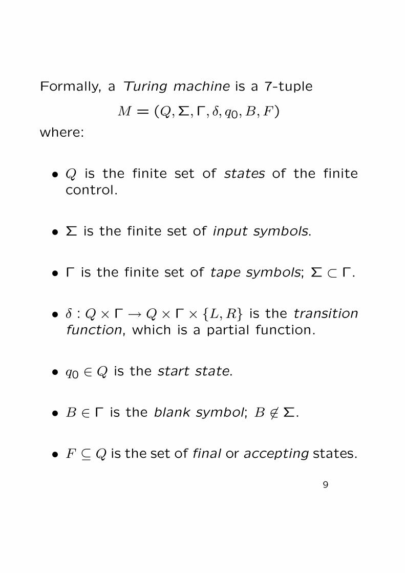
Formally, a Turing machine is a 7-tuple

M = (Q,Σ,Γ, δ, q0, B, F )

where:

• Q is the finite set of states of the finite

control.

• Σ is the finite set of input symbols.

• Γ is the finite set of tape symbols; Σ ⊂ Γ.

• δ : Q × Γ → Q × Γ × {L, R} is the transition

function, which is a partial function.

• q0 ∈ Q is the start state.

• B ∈ Γ is the blank symbol; B 6∈ Σ.

• F ⊆ Q is the set of final or accepting states.

9

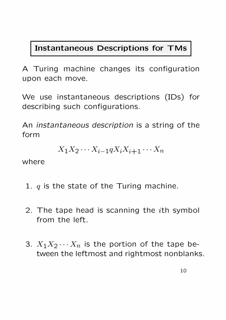
Instantaneous Descriptions for TMs

A Turing machine changes its configuration

upon each move.

We use instantaneous descriptions (IDs) for

describing such configurations.

An instantaneous description is a string of the

form

X1X2 · · ·Xi−1qXiXi+1 · · ·Xn

where

1. q is the state of the Turing machine.

2. The tape head is scanning the ith symbol

from the left.

3. X1X2 · · ·Xn is the portion of the tape be-

tween the leftmost and rightmost nonblanks.

10

The Moves and Language of a TM

We useM

to designate a move of a Turing

machine M from one ID to another.

If δ(q, Xi) = (p, Y, L), then:

X1X2 · · ·Xi−1qXiXi+1 · · ·XnM

X1X2 · · ·Xi−2pXi−1Y Xi+1 · · ·Xn

If δ(q, Xi) = (p, Y, R), then:

X1X2 · · ·Xi−1qXiXi+1 · · ·XnM

X1X2 · · ·Xi−1Y pXi+1 · · ·Xn

The reflexive-transitive closure ofM

is denoted

by∗

M.

A Turing machine M = (Q,Σ,Γ, δ, q0, B, F ) ac-

cepts the language

L(M) = {w ∈ Σ∗ : q0w∗

Mαpβ, p ∈ F, α, β ∈ Γ∗}

11

Example: A TM for {0n1n : n ≥ 1}

M = ({q0, q1, q2, q3, q4}, {0,1}, {0,1, X, Y, B}, δ, q0, B, {q4})

where δ is given by the following table:

0 1 X Y B

→ q0 (q1, X, R) (q3, Y, R)q1 (q1,0, R) (q2, Y, L) (q1, Y, R)q2 (q2,0, L) (q0, X, R) (q2, Y, L)q3 (q3, Y, R) (q4, B, R)

? q4

We can also represent M by the following tran-

sition diagram:

/Y Y

/Y Y

/Y Y

0/0

X/0

/X X

/B B

/ Y1

/Y Y

0/0Start

q q q

q q

0 1 2

3 4

12

Example: A TM With “Output”

The following Turing machine computes

m.− n = max(m − n,0)

0 1 B

→ q0 (q1, B, R) (q5, B, R)q1 (q1,0, R) (q2,1, R)q2 (q1,1, L) (q2,1, R) (q4, B, L)q3 (q3,0, L) (q3,1, L) (q0, B, R)q4 (q4,0, L) (q4, B, L) (q6,0, R)q5 (q5, B, R) (q5, B, R) (q6, B, R)

? q6

The transition diagram is as follows:

/1 1/0 B

1 / B

1 / B

0/0

/1 1

/B B

/B B

0/0/0 B

1 / B

B / 0

0/0 /1 1

/B B

Startq q q

q q

0 1 2

q

q0 / 1

4

3

5 6

13

Acceptance by Halting

A Turing machine halts if it enters a state q,

scanning a tape symbol X, and there is no

move in this situation, i.e., δ(q, X) is undefined.

We can always assume that a Turing machine

halts if it accepts, as we can make δ(q, X) un-

defined whenever q is an accepting state.

Unfortunately, it is not always possible to re-

quire that a Turing machine halts even if it

does not accept.

Recursive language: there is a TM, correspond-

ing to the concept of algorithm, that halts

eventually, whether it accepts or not.

Recursively enumerable language: there is a

TM that halts if the string is accepted.

Decidable problem: there is an algorithm for

solving it.

14

Alternative Models for Turing Machines

Turing-machine programming techniques: stor-

age in the state, multiple tape tracks, subrou-

tines, . . .

Extensions: multiple tapes, non-determinism,

. . .

Restrictions: semi-infinite tape, multiple stacks,

counters, . . .

All these models are equivalent: they accept

the recursively enumerable languages (Church-

Turing thesis, 1936).

15

Turing Machines and Computers

Simulating a Turing machine by a computer:

it suffices to have enough memory to simulate

the infinite tape.

Simulating a computer by a Turing machine:

multiple tapes (memory, instruction counter,

memory address, computer’s input file, and

scratch) plus simulation of the instruction cy-

cle.

The simulating multitape Turing machine needs

an amount of steps that is at most some poly-

nomial, namely n3, in the number n of steps

taken by the simulated computer.

From now on: computer = Turing machine.

16

9: Undecidability

Goal: Prove undecidable the recursively enu-

merable language Lu consisting of pairs (M, w)

such that:

• M is a Turing machine (suitably coded, in

binary) with input alphabet {0,1}.

• w is a string of 0s and 1s.

• M accepts input w.

If this problem with binary inputs is undecid-

able, then surely the more general problem,

where the Turing machines may have any al-

phabet, is undecidable.

First step: codify a Turing machine as a string

of 0s and 1s, and exhibit a language that is

not even recursively enumerable, namely Ld.

17

Codes for Turing Machines

We need to assign integers to all the binary

strings so that each integer corresponds to one

string and vice versa: ε is the first string, 0 the

second, 1 the third, 00 the fourth, 01 the fifth,

and so on.

Equivalently, strings are ordered by length, and

strings of equal length are ordered lexicograph-

ically.

We will refer to the ith string as wi.

We now want to represent Turing machines

with input alphabet {0,1} by binary strings,

so that we can identify Turing machines with

integers and refer to the ith Turing machine

as Mi.

18

To represent a Turing machine

M = (Q, {0,1},Γ, δ, q1, B, F}

as a binary string, we must first assign integers

to the states, tape symbols, and directions L

and R:

• Assume the states are q1, q2, . . . , qr for some

r. The start state is q1, and the only ac-

cepting state is q2.

• Assume the tape symbols are X1, X2, . . . , Xs

for some s. Then: 0 = X1, 1 = X2, and

B = X3.

• L = D1 and R = D2.

19

Encode the transition rule

δ(qi, Xj) = (qk, X`, Dm) by 0i10j10k10`10m.

Note that there are no two consecutive 1s.

Encode an entire Turing machine by concate-

nating, in any order, the codes Ci of its transi-

tion rules, separated by 11: C111C211 · · ·Cn−111Cn.

Ex.: M = ({q1, q2, q3}, {0,1}, {0,1, B}, δ, q1, B, {q2})

where δ is defined by: δ(q1,1) = (q3,0, R),

δ(q3,0) = (q1,1, R), δ(q3,1) = (q2,0, R), and

δ(q3, B) = (q3,1, L).

Codes for the transition rules:

0100100010100

0001010100100

00010010010100

0001000100010010

Code for M :

010010001010011000101010010011

00010010010100110001000100010010

20

Given a Turing machine M with code wi, we

can now associate an integer to it: M is the

ith Turing machine, referred to as Mi.

Many integers do no correspond to any Turing

machine at all. Examples: 11001 and 001110.

If wi is not a valid TM code, then we shall take

Mi to be the Turing machine (with one state

and no transitions) that immediately halts on

any input. Hence L(Mi) = ∅ if wi is not a valid

TM code.

21

The Diagonalisation Language Ld

The diagonalisation language Ld is the set of

strings wi such that wi 6∈ L(Mi).

That is, Ld contains all strings w such that

the Turing machine M with code w does not

accept w.

Consider the matrix with Turing machine in-

dices i in the rows and string indices j in the

columns, where the cell for row i and column

j tells whether Mi accepts wj, ”yes” being de-

noted by 1 and ”no” by 0. The diagonal values

tell whether Mi accepts wi. The strings of Ld

correspond to the 0s of the diagonal.

Is it possible that the diagonal complement is

a row? No, because the diagonal complement

disagrees with every row in some column.

Hence Ld is not recursively enumerable and

cannot be accepted by any Turing machine.

22

Recursive Languages

A language L is recursive if L = L(M) for some

Turing machine M such that:

• If w ∈ L, then M accepts w (and halts).

• If w 6∈ L, then M does not accept w but

eventually halts.

Such a Turing machine corresponds to our in-

formal notion of an ”algorithm”.

The problem (of acceptance of L) is decidable

if L is recursive, and undecidable otherwise.

23

Classes of Languages

• Recursive = decidable:

their Turing machine always halt.

• Recursively enumerable but not recursive:

their Turing machines halt if they accept.

Example: Lu.

• Non recursively enumerable (non-RE):

there are no Turing machines for them.

Example: Ld.

24

Property of Recursive Languages

The recursive languages are closed under com-

plementation:

Theorem 9.3: If L is a recursive language,

then L is recursive.

Proof: If L is recursive, then L = L(M) for

some Turing machine M that always halts. Trans-

form M into M ′ such that M ′ accepts what M

does not accept, and vice versa. So M ′ always

halts and accepts L. Hence L is recursive.

Consequence: If L is RE, but L is not RE, then

L cannot be recursive.

25

Property of RE Languages

Theorem 9.4: If L and L are RE, then L is

recursive (and so is L, by Theorem 9.3).

Proof: Let L = L(M1) and L = L(M2). Con-

struct a Turing machine M that simulates M1

and M2 in parallel (using two tapes and two

heads). If the input to M is in L, then M1

accepts it and halts, hence M also accepts it

and halts. If the input to M is not in L, then

M2 accepts it and halts, hence M halts with-

out accepting it. Hence M halts on every input

and L(M) = L, so L is recursive.

26

L and L

There are only four ways of placing L and L:

• Both L and L are recursive.

• Neither L nor L is RE.

• L is RE but not recursive, and L is not RE.

• L is RE but not recursive, and L is not RE.

Indeed, it is impossible that one language (L

or L) is recursive and the other is in either of

the other two classes (by Theorem 9.3).

It is also impossible that both languages are

RE but not recursive (by Theorem 9.4).

27

The Universal Language

The universal language Lu is the set of binary

strings that encode a pair (M, w) (by putting

111 between the code for M and w) where

w ∈ L(M).

There is a Turing machine U , often called the

universal Turing machine, such that Lu = L(U).

It has three tapes: one for the code of (M, w),

one for the code of the simulated tape of M ,

and one for the code of the state of M . Thus

U simulates M on w, and U accepts (M, w) if

and only if M accepts w. Hence Lu is RE.

Any Turing machine M may not halt when the

input string w is not in the language, thus

U will have the same behaviour as M on w.

Hence Lu is RE but not recursive.

28

The Halting Problem

Given a Turing machine M , define H(M) to be

the set of strings w such that M halts on input

w, regardless of whether or not M accepts w.

The halting problem is the set of pairs (M, w)

such that w ∈ H(M). This problem (or lan-

guage) also is recursively enumerable but not

recursive.

29

Closure Properties of Recursive Languages

The recursive languages are closed under the

following operations:

• Union.

• Intersection.

• Concatenation.

• Kleene closure.

30

Closure Properties of RE Languages

The recursively enumerable (RE) languages are

closed under the following operations:

• Union.

• Intersection.

• Concatenation.

• Kleene closure.

31

Recursive and RE Languages

Given a recursive language and a recursively

enumerable (RE) language:

• Union: RE.

• Intersection: RE.

• Concatenation: RE.

• Kleene closure: RE.

• If L1 is recursive and L2 is RE,

then L2 − L1 is RE and L1 − L2 is not RE.

32

Problem Reduction

Recall ”Problem Reduction” of Chapter 8.

If P1 reduces to P2,

then P2 is at least as hard as P1.

Theorem 9.7: If P1 reduces to P2, then:

• If P1 is undecidable, then so is P2.

• If P1 is non-RE, then so is P2.

33

Examples of Undecidable Problems

Theorem 9.11: All non-trivial properties of

RE languages are undecidable. (Rice, 1953)

All problems about Turing machines that in-

volve only the language that the TM accepts

are undecidable.

Examples:

Is the language accepted by the TM empty?

Is the language accepted by the TM finite?

Is the language accepted by the TM regular?

Is the language accepted by the TM a CFL?

Does the language accepted by the TM con-

tain the string ”ab”?

Does the language accepted by the TM con-

tain all even numbers?

34

Example of Decidable Problems

Fortunately, not everything is undecidable! Some

problems about the states of the Turing ma-

chine, rather than about the language it ac-

cepts, are decidable.

Examples:

Does the TM have five states?

Is there an input such that the TM makes at

least five moves?

35