introductionintroduction we say a geodesic metric space xis gromov hyperbolic, or -hyperbolic, if...
TRANSCRIPT

RANDOM WALKS ON WEAKLY HYPERBOLIC GROUPS
JOSEPH MAHER, GIULIO TIOZZO
Abstract. Let G be a countable group which acts by isometries on aseparable, but not necessarily proper, Gromov hyperbolic space X. Wesay the action of G is weakly hyperbolic if G contains two independenthyperbolic isometries. We show that a random walk on such G convergesto the Gromov boundary almost surely. We apply the convergence resultto show linear progress and linear growth of translation length, withoutany assumptions on the moments of the random walk.
If the action is acylindrical, and the random walk has finite entropyand finite logarithmic moment, we show that the Gromov boundary withthe hitting measure is the Poisson boundary.
1. Introduction
We say a geodesic metric space X is Gromov hyperbolic, or δ-hyperbolic,if there is a number δ > 0 for which every geodesic triangle in X satisfies theδ-slim triangle condition, i.e. any side is contained in a δ-neighbourhood ofthe other two sides. Throughout this paper we will assume that the spaceX is separable, i.e. it contains a countable dense set, but we will not assumethat X is proper or locally compact. For example, any countable simplicialcomplex satisfies these conditions.
Let G be a countable group which acts by isometries on X. We saythe action of G on X is non-elementary if G contains a pair of hyperbolicisometries with disjoint fixed point sets in the Gromov boundary. We sayG is weakly hyperbolic if it admits a non-elementary action by isometries onsome Gromov hyperbolic space X. In this case, a natural boundary for thegroup is given by the Gromov boundary ∂X of X, which however need notbe compact.
Several widely studied group actions are weakly hyperbolic in this sense,in particular:
• Hyperbolic and relatively hyperbolic groups;• Mapping class groups, acting on the curve complex;• Out(Fn) acts on various Gromov hyperbolic simplicial complexes, for
example the complex of free factors or the complex of free splittings;• Right-angled Artin groups acting on their extension graphs;• Finitely generated subgroups of the Cremona group.
2010 Mathematics Subject Classification. 60G50, 20F67, 57M60.
1

2 JOSEPH MAHER, GIULIO TIOZZO
In particular, all acylindrically hyperbolic groups are weakly hyperbolic, seeSection 1.2 for further discussion and more examples.
In this paper, we shall consider random walks on weakly hyperbolicgroups, constructed by choosing products of random group elements. Aprobability distribution µ on G determines a random walk on G, by takingthe product
wn := g1g2 . . . gn
where the gi are independent identically distributed elements of G, withdistribution µ. A choice of basepoint x0 ∈ X determines an orbit mapsending g 7→ gx0, and we can project the random walk on G to X byconsidering the sequence (wnx0)n∈N, which we call a sample path. Thesupport of µ consists of all group elements g for which µ(g) > 0. We say ameasure µ on G is non-elementary if the semigroup generated by the supportof µ contains a pair of hyperbolic isometries with disjoint fixed point sets.
1.1. Results. The first result we establish is that sample paths convergealmost surely in the Gromov boundary:
Theorem 1.1. Let G be a countable group of isometries of a separableGromov hyperbolic space X, and let µ be a non-elementary probability dis-tribution on G. Then, for any basepoint x0 ∈ X, almost every sample path(wnx0)n∈N converges to a point ω+ ∈ ∂X. The resulting hitting measure νis non-atomic, and is the unique µ-stationary measure on ∂X.
We use the convergence to the boundary result to show the followinglinear progress, or positive drift, result. Recall that a measure µ has finitefirst moment if
∫G dX(x0, gx0) dµ(g) <∞.
Theorem 1.2. Let G be a countable group of isometries of a separableGromov hyperbolic space X, and let µ be a non-elementary probability dis-tribution on G, and x0 ∈ X a basepoint. Then there is a constant L > 0such that for almost every sample path we have
lim infn→∞
dX(x0, wnx0)
n> L > 0.
Furthermore, if µ has finite first moment, then the limit
limn→∞
dX(x0, wnx0)
n= L > 0
exists almost surely. Finally, if the support of µ is bounded in X, then thereare constants c < 1,K and L > 0 such that
P(dX(x0, wnx0) 6 Ln) 6 Kcn
for all n.
Note that the constants L, K, and c depend on the choice of the measureµ. Moreover, the first statement also implies that
limn→∞
P(dX(x0, wnx0) 6 Ln) = 0

RANDOM WALKS ON WEAKLY HYPERBOLIC GROUPS 3
(for a possibly different constant L). If we assume that µ has finite first mo-ment with respect to the distance function dX , then we obtain the followinggeodesic tracking result.
Theorem 1.3. Let G be a countable group which acts by isometries on aseparable Gromov hyperbolic space X with basepoint x0, and let µ be non-elementary probability distribution on G, with finite first moment. Then foralmost every sample path (wnx0)n∈N there is a quasigeodesic ray γ whichtracks the sample path sublinearly, i.e.
limn→∞
dX(wnx0, γ)
n= 0, almost surely.
If the support of µ is bounded in X, then in fact the tracking is logarithmic,i.e.
lim supn→∞
dX(wnx0, γ)
log n<∞, almost surely.
Finally, we investigate the growth rate of translation length of groupelements arising from the sample paths.
Theorem 1.4. Let G be a countable group which acts by isometries on aseparable Gromov hyperbolic space X, and let µ be a non-elementary prob-ability distribution on G. Then the translation length τ(wn) of the groupelement wn grows at least linearly in n, i.e.
P(τ(wn) 6 Ln)→ 0 as n→∞,for some constant L strictly greater than zero.
If the support of µ is bounded in X, then there are constants c < 1,K andL > 0, such that
P(τ(wn) 6 Ln) 6 Kcn
for all n.
Recall that the translation length τ(g) of an isometry g of X is definedas
τ(g) := limn→∞
1ndX(x0, g
nx0).
As an element with non-zero translation length is a hyperbolic (= loxo-dromic) isometry, this shows that the probability that a random walk oflength n gives rise to a hyperbolic isometry tends to one as n tends toinfinity.
The Poisson boundary of acylindrically hyperbolic groups. A special classof weakly hyperbolic groups are the acylindrically hyperbolic groups. In thiscase, we show that we may identify the Gromov boundary (∂X, ν) with thePoisson boundary.
Recall that a group G acts acylindrically on a Gromov hyperbolic spaceX, if for every K > 0 there are numbers R and N , which both dependon K, such that for any pair of points x and y in X, with dX(x, y) > R,there are at most N group elements g in G such that dX(x, gx) 6 K anddX(y, gy) 6 K.
4 JOSEPH MAHER, GIULIO TIOZZO
Theorem 1.5. Let G be a countable group of isometries which acts acylin-drically on a separable Gromov hyperbolic space X, let µ be a non-elementaryprobability distribution on G with finite entropy and finite logarithmic mo-ment, and let ν be the hitting measure on ∂X. Then (∂X, ν) is the Poissonboundary of (G,µ).
1.2. Examples and discussion.
Word hyperbolic groups. The simplest example of a weakly hyperbolicgroup is a (finitely generated) Gromov hyperbolic group acting on its Cay-ley graph, which by definition is a δ-hyperbolic space, and so any non-elementary Gromov hyperbolic group is weakly hyperbolic. Convergence ofsample paths to the Gromov boundary in this case is due to Kaimanovich[Kai94], who also shows that the Gromov boundary may be identified withthe Poisson boundary and the hitting measure is the unique µ-stationarymeasure. Note that in this case the space is locally compact, and the bound-ary is compact.
Relatively hyperbolic groups. The Cayley graph of a relatively hyperbolicgroup is δ-hyperbolic with respect to an infinite generating set, and so thesegroups are also weakly hyperbolic, but in this case the space on which thegroup acts need not be proper. In this case, convergence to the boundarywas shown by Gautero and Matheus [GM12], who also covered the case ofgroups acting on R-trees. More recently, group actions on (locally infinite)trees have been considered by Malyutin and Svetlov [MS14].
There are then groups which are weakly hyperbolic, but not relatively hy-perbolic, the two most important examples being the mapping class groupsof surfaces, and Out(Fn).
Mapping class groups. The mapping class group Mod(S) of a surface S ofgenus g with p punctures acts on the curve complex C(S), which is a locallyinfinite simplicial complex. As shown by Masur and Minsky [MM99], thecurve complex is δ-hyperbolic, and moreover, the action is acylindrical, bywork of Bowditch [Bow08], so we can apply our techniques to get convergenceand the Poisson boundary.
Convergence to the boundary of the curve complex also follows from workof Kaimanovich and Masur [KM96] and Klarreich [Kla], using the action ofMod(S) on Teichmuller space (which is locally compact, but not hyperbolic).Indeed, Kaimanovich and Masur show that random walks on the mappingclass group converge to points in Thurston’s compactification of Teichmullerspace PMF , and then Klarreich (see also Hamenstadt [Ham06]) shows therelation between PMF and the boundary of the curve complex. Our ap-proach does not use fine properties of Teichmuller geometry. A third ap-proach is to consider the action of Mod(S) on Teichmuller space with theWeil-Petersson metric, which is a non-proper CAT(0) space. By work ofBestvina, Bromberg and Fujiwara [BBF10], this space has finite telescopic

RANDOM WALKS ON WEAKLY HYPERBOLIC GROUPS 5
dimension, and one may then apply the results of Bader, Duchesne andLecureux [BDL14].
We remark that C(S) does not possess a CAT(0) metric, since it is ho-motopic to a wedge of spheres (Harer [Har86]); in fact, Kapovich and Leeb[KL96] showed that the mapping class group (of genus at least 3) does notact freely cocompactly on a CAT(0) space, though it is still open as towhether there is a proper CAT(0) space on which the mapping class groupacts by isometries; Bridson [Bri12] showed that any such action must haveelliptic or parabolic Dehn twists.
Out(Fn). The outer automorphism group of a non-abelian free group,Out(Fn), acts on a number of distinct Gromov hyperbolic spaces, as shownby Bestvina and Feighn [BF10,BF14] and Handel and Mosher [HM13], andso is weakly hyperbolic. Similarly to the case of Mod(S), convergence to theboundary also follows by considering the action of Out(Fn) on the (locallycompact) outer space, as shown by Horbez [Hor14].
Right-angled Artin groups. A right-angled Artin group acts by simplicialisometries on its extension graph, which has infinite diameter as long asthe group does not split as a non-trivial direct product, and is not quasi-isometric to Z. Kim and Koberda showed that the extension graph is a (non-locally compact) quasi-tree [KK13], and in fact the action is acylindrical[KK14].
Finitely generated subgroups of the Cremona group. Manin [Man74] showedthat the Cremona group acts faithfully by isometries on an infinite-dimensionalhyperbolic space, known as the Picard-Manin space, which is not separable.However, any finite-generated subgroup preserves a totally geodesic closedsubspace, which is separable, see for example Delzant and Py [DP12].
Acylindrically hyperbolic groups. The definition of an acylindrical groupaction is due to Sela [Sel97] for trees, and Bowditch [Bow08] for generalmetric spaces, see Osin [Osi13] for a discussion and several examples ofacylindrical actions on hyperbolic spaces. As every acylindrically hyperbolicgroup is also weakly hyperbolic, this gives a number of additional examplesof weakly hyperbolic groups which are not necessarily relatively hyperbolic;for example, all one relator groups with at least three generators, see [Osi13]for many other examples.
Isometries of CAT(0) spaces. Even though not all CAT(0) spaces are hy-perbolic, the two theories overlap in many cases. For isometries of generalCAT(0) spaces, Karlsson and Margulis [KM96] proved boundary conver-gence and identified the Poisson boundary. More recently, boundaries ofCAT(0) cube complexes have been studied by Nevo and Sageev [NS13], and(not necessarily proper) CAT(0) spaces of finite telescopic dimension byBader, Duchesne and Lecureux [BDL14].
Once we have proved convergence to the boundary, we apply this to showpositive drift. In the locally compact case, positive drift results go back toGuivarc’h [Gui80]. In particular, when the space on which G acts is proper,

6 JOSEPH MAHER, GIULIO TIOZZO
positive drift follows from non-amenability of the group, but this need notbe the case for non-proper spaces. In the curve complex case, linear progressis due to Maher [Mah10a].
We then show the sublinear tracking results, using work of Tiozzo [Tio12].Sublinear tracking can be thought of as a generalization of Oseledec’s mul-tiplicative ergodic theorem [Ose68]. In our context, these results go back toGuivarc’h [Gui80], and are known for groups of isometries of CAT(0) spacesby Karlsson and Margulis [KM96], and for Teichmuller space by Duchin[Duc05]. Sublinear tracking on hyperbolic groups is due to Kaimanovich[Kai87, Kai94]; moreover, Karlsson and Ledrappier [KL06, KL07] proved alaw of large numbers on general (proper) metric spaces using horofunctions.
Note that these results can be used to prove convergence to the boundaryonce one knows that the drift is positive. In the above-mentioned cases, thespace is meant to be proper, so positive drift follows from non-amenabilityof the group, while a new argument is needed in general.
In this paper we give an argument for the non-proper weakly hyperboliccase, where sublinear tracking and positive drift follow from convergence tothe boundary. Note that in our approach we use horofunctions, and indeed[KL06] can be used to simplify our proofs if one assumes positive drift.Recently (after the first version of this paper appeared), Mathieu and Sisto[MS14] provided a different argument for positive drift in the acylindricalcase.
Logarithmic tracking was previously known for random walks on trees,due to Ledrappier [Led01], on hyperbolic groups, due to Blachere, Haıssinskyand Mathieu [BHM11], and on relatively hyperbolic groups, due to Sisto[Sis13].
Finally we show that the translation length grows linearly, which in par-ticular shows that the probability that a random walk gives rise to a hyper-bolic element tends to one. This generalizes earlier work of Rivin [Riv08],Kowalski [Kow08], Maher [Mah11] and Sisto [Sis11].
The methods in this paper build on previous work of Calegari and Maher[CM15], which showed convergence results with stronger conditions on Xand µ.
1.3. Outline of the argument. To explain the argument in the proof ofTheorem 1.1, we briefly remind the reader of the standard argument forconvergence to the boundary for a random walk on a group G acting on alocally compact δ-hyperbolic space X. The argument ultimately goes backto Furstenberg [Fur63], who developed it for Lie groups.
Measures on the Gromov boundary. Let µ be the probability distributionon G generating the random walk. The first step is to find a µ-stationarymeasure ν on the Gromov boundary ∂X, and then apply the martingale con-vergence theorem to show that for almost every sample path ω = (wn)n∈N,the sequence of measures (wnν)n∈N converges to some measure νω in P(∂X),

RANDOM WALKS ON WEAKLY HYPERBOLIC GROUPS 7
the space of probability measures on ∂X. One then uses geometric prop-erties of the action of G on X to argue that νω is a δ-measure δλ for somepoint λ ∈ ∂X, almost surely, and that the image of the sample path underthe orbit map (wnx0)n∈N converges to λ.
This argument uses local compactness in an essential way in the firststep. For a locally compact hyperbolic space X, the Gromov boundary ∂Xis compact, as is X ∪ ∂X. The space of probability measures on ∂X is alsocompact, and so the existence of a µ-invariant measure on X just followsfrom taking weak limits. In the non-locally compact case, the Gromovboundary ∂X, and X ∪ ∂X, need not be compact, as seen in the followingexample.
Example 1.6 (Countable wedge of rays). A ray is a half line R+ = x ∈R : x > 0, with basepoint 0. Let X be the wedge product of countablymany rays. This space is a tree, and so is δ-hyperbolic, and is not locallycompact at the basepoint. The Gromov boundary is homeomorphic to N withthe discrete metric, and is not compact.
The horofunction boundary. In order to address this issue, we shall con-sider the horofunction boundary of X, which was also initially developed byGromov [BGS85], and has proved a useful tool in studying random walks,see for example Karlsson-Ledrappier [KL06, KL07] and Bjorklund [Bjo10].We now give a brief description of this construction, giving full details inSection 3.
Let X be a metric space, and x0 a basepoint. For each point x in X, onedefines the horofunction ρx determined by x to be the function ρx : X → R
ρx(z) := dX(x, z)− dX(x, x0).
This gives an embedding of X in the space C(X) of (Lipschitz-) continuousfunctions on X, which we shall consider with the compact-open topology(we emphasize that we use uniform convergence on compact sets, not uni-form convergence on bounded sets). With this topology, the closure of ρ(X)in C(X) is compact, even if X is not locally compact; it is called the horo-
function compactification of X and denoted by Xh. In particular, there is a
µ-stationary measure ν on Xh.
We now consider a basic but fundamental example in detail.
Example 1.7 (R). Consider X = R, with the usual metric. In this case
the horofunction boundary Xh
consists of ρ(X) together with precisely twoadditional functions, namely ρ∞(x) := −x, and ρ−∞(x) := x.
This example turns out to be very important in our case; indeed, if X isGromov hyperbolic, then the restriction of an arbitrary horofunction to ageodesic is equal (up to a bounded additive error) to one of the horofunctionsdescribed above, i.e. ρx or ρ±∞.
In Example 1.6, the horofunction boundary equals the Gromov boundaryas a set, but the topology is different: namely, any sequence of horofunctions

8 JOSEPH MAHER, GIULIO TIOZZO
(ρxn)n∈N corresponding to a sequence of points (xn)n∈N which leaves everycompact set converges to the horofunction ρx0 associated to the basepointx0.
The Gromov boundary may be recovered from the horofunction boundaryby identifying functions which differ by a bounded amount, but in generalthe horofunction boundary may be larger than the Gromov boundary, andis not a quasi-isometry invariant of the space.
Example 1.8. Consider X = Z×Z/2Z, with the L1-metric, dX((x, i), (y, j)) =|x− y| + |i− j|. Then the sequences ρn,0 and ρn,1 have different values on(0, 1), and so converge to distinct horofunctions, and in fact in this case thehorofunction boundary consists of the product of the Gromov boundary withZ/2Z.
We shall distinguish two different types of horofunctions. We say a ho-rofunction h is finite if infx∈X h(x) > −∞, and is infinite if inf h = −∞.
This partitions Xh
into two subsets: we shall write XhF for the set of finite
horofunctions, and Xh∞ for the set of infinite horofunctions.
The local minimum map. We shall now construct a map from the horo-function boundary to the Gromov boundary. Recall that the restriction of ahorofunction h to a geodesic γ in X is coarsely equal to one of the standardhorofunctions on R: in particular, it has (coarsely) at most one local mini-mum on γ. Thus, if h is bounded below on γ, we can map h to the location
where it attains its minimum, getting a map φ : XhF → X. On the other
hand, if the horofunction is not bounded below, then we can pick a sequence(xn) of points for which the value of the horofunction tends to −∞; it turnsout that such a sequence converges to a unique point in the Gromov bound-ary, and the limit is independent of the choice of (xn). Thus, we can extend
φ to a map φ : Xh → X ∪∂X. We show that this map is continuous on X
h∞
and G-equivariant, and that the stationary measure ν is supported on the
infinite horofunctions Xh∞. Therefore the stationary probability measure ν
on Xh
restricts to a probability measure on Xh∞, and pushes forward to
a µ-stationary probability measure ν on ∂X. We may then complete theargument using with the geometric properties of the action of G on ∂X.
Plan of the paper. In Section 2, we review some useful material aboutGromov hyperbolic spaces, and fix notation. In Section 3, we develop theproperties of the horofunction boundary that we will use, including the localminimum map, and the behaviour of shadows. In these initial sections wegive complete proofs in the non-proper case of certain statements that arealready known in the proper case. In Section 4, we use the horofunctionboundary to show that almost every sample path converges to the Gromovboundary. In Section 5, we use the convergence to the boundary result toshow results on positive drift, sublinear tracking, and the growth rate oftranslation distance, and then finally in Section 6 we show that if the action

RANDOM WALKS ON WEAKLY HYPERBOLIC GROUPS 9
of G is acylindrical, and µ has finite entropy, then the Gromov boundarywith the hitting measure is the Poisson boundary for the random walk.
1.4. Acknowledgements. We would like to thank Jason Behrstock, DannyCalegari, Romain Dujardin, Camille Horbez, Vadim Kaimanovich, AndersKarlsson, Andrei Malyutin and Samuel Taylor for helpful conversations. Wealso thank the referee for the useful comments on the manuscript. The firstauthor gratefully acknowledges the support of the Simons Foundation andPSC-CUNY. The authors would like to thank the referee for his helpfulcomments and suggestions.
2. Background on δ-hyperbolic spaces
Let X be a Gromov hyperbolic space, i.e. a geodesic metric space whichsatisfies the δ-slim triangles condition. We will not assume that X is proper,i.e. that closed balls are compact, but we will always assume that it isseparable, i.e. that it contains a dense countable subset. We shall write dXfor the metric on X, and BX(x, r) for the closed ball of radius r about thepoint x in X. We shall now recall a few facts on the geometry of X.
2.1. Notation. We shall write f(x) = O(δ) to mean that the absolutevalue of the function f is bounded by a number which only depends on δ,though this need not be a linear multiple of δ. Similarly, we shall writeA = B +O(δ) to mean that the difference between A and B is bounded bya constant, which depends only on δ.
2.2. Coarse geometry. Recall that the Gromov product in a metric spaceis defined to be
(x · y)x0 := 12(dX(x0, x) + dX(x0, y)− dX(x, y)).
In a δ-hyperbolic space, for all points x0, x and y, the Gromov product(x · y)x0 is equal to the distance from x0 to a geodesic from x to y, up to anadditive error of at most δ: if we write [x, y] for a choice of geodesic from xto y, then
(1) dX(x0, [x, y]) = (x · y)x0 +O(δ),
see e.g. [BH99, III.H 1.19]. Moreover, for any three points x, y, z ∈ X onehas the following inequality
(2) (x · y)x0 > min(x · z)x0 , (y · z)x0 −O(δ),
which we shall refer to as the triangle inequality for the Gromov product.We now recall the definition of the Gromov boundary of X, which we shall
write as ∂X. We say that a sequence (xn)n∈N ⊆ X is a Gromov sequence if(xm · xn)x0 tends to infinity as minm,n tends to infinity. We say that twoGromov sequences (xn)n∈N and (yn)n∈N are equivalent if (xn · yn)x0 tendsto infinity as n tends to infinity. The Gromov boundary ∂X is defined asthe set of equivalence classes of Gromov sequences.

10 JOSEPH MAHER, GIULIO TIOZZO
We can extend the Gromov product to the boundary by
(x · y)x0 = sup lim infm,n→∞
(xm · yn)x0 ,
where the supremum is taken over all sequences (xm)m∈N → x and (yn)n∈N →y. With this definition, the triangle inequality (2) also holds for any threepoints x, y, z in X ∪ ∂X, but with a larger additive constant O(δ) (see e.g.[BH99, III.H Remark 3.17(4)]).
The Gromov product on the boundary may be used to define a completemetric on ∂X, see Bridson and Haefliger [BH99, III.H.3] for the proper case,and Vaisala [Vai05] for the non-proper case. Moreover, the space X ∪ ∂Xcan be equipped with a topology such that the relative topologies on both Xand ∂X are equal respectively to the usual topology on X, and the above-mentioned metric topology on ∂X.
If U ⊂ X we shall write Uδ
for the closure of U in X∪∂X. If X is proper,then ∂X is compact, but it need not be compact if X is not proper. However,a bounded set does not have limit points in the Gromov boundary, i.e. for
BX(x0, r) = x ∈ X : dX(x0, x) 6 r we have BX(x0, r)δ
= BX(x0, r).
2.3. Quasigeodesics. Let I be a connected subset of R, and let X be ametric space. A (Q, c)-quasigeodesic is a (not necessarily continuous) mapγ : I → X such that for all s and t in I,
1
Q|t− s| − c 6 dX(γ(s), γ(t)) 6 Q |t− s|+ c.
If I = R, then we will call the quasigeodesic γ a bi-infinite quasigeodesic.If I = [0,∞), then we shall call γ a quasigeodesic ray based at γ(0). If themetric space is δ-hyperbolic, then quasigeodesics have the following stabilityproperty, which is often referred to as the Morse Lemma (see [BH99, III.H1.7], [Vai05, Theorem 6.32]).
Proposition 2.1. Let X be a δ-hyperbolic space. Given numbers Q and c,there is a number L such that for any two points x and y in X∪∂X, any two(Q, c)-quasigeodesics connecting x and y are contained in L-neighbourhoodsof each other.
We shall refer to a choice of constant L in Proposition 2.1 above as aMorse constant for the quasi-geodesic constants Q and c.
For any choice of basepoint x0 and every point x in the boundary there isa quasigeodesic ray based at x0 which converges to the point x, and any twopoints in the boundary are connected by a bi-infinite quasigeodesic. In fact,the quasigeodesics may be chosen to have quasigeodesic constants Q and cbounded above in terms of the hyperbolicity constant δ, independently ofthe choice of basepoint or boundary points, see e.g. Bonk and Schramm[BS00, Proposition 5.2] or Kapovich and Benakli [KB02, Remark 2.16]. Bychoosing Q and c sufficiently large, we may assume that we have chosen theseconstants so that at least one of the (Q, c)-quasigeodesics is continuous, seee.g. Bridson and Haefliger [BH99, III.H.1].

RANDOM WALKS ON WEAKLY HYPERBOLIC GROUPS 11
2.4. Nearest point projection. We will use the fact that in a δ-hyperbolicspace nearest point projection onto a geodesic γ is coarsely well defined, i.e.there is a constant K2, which only depends on δ, such that if p and q arenearest points on γ to x, then dX(p, q) 6 K2.
We will make use of the following reverse triangle inequality.
Proposition 2.2. Let γ be a geodesic in X, y ∈ X a point, and p a nearestpoint projection of y to γ. Then for any z ∈ γ we have
(3) dX(y, z) = dX(y, p) + dX(z, p) +O(δ),
and furthermore, any geodesic from z to y passes within distance O(δ) of p.
Proof. The upper bound for dX(y, z) is immediate from the usual triangleinequality. To prove the lower bound, by the definition of nearest pointprojection,
dX(y, p) = dX(y, [p, z]).
Recall that by (1),
dX(y, p) 6 (p · z)y +O(δ),
and writing out the Gromov product, we get
dX(y, p) 61
2
(dX(y, p) + dX(y, z)− dX(p, z)
)+O(δ),
which yields
dX(y, z) > dX(y, p) + dX(p, z)−O(δ),
as required. This implies that a path consisting of [y, p] ∪ [p, z] is a (1, C)-quasigeodesic for some C = O(δ), and so by stability of quasigeodesics in aδ-hyperbolic space, this path is contained in an O(δ)-neighbourhood of anygeodesic [y, z] from y to z, so in particular, the distance from p to a [y, z] isat most O(δ).
Finally we show that if two points x and y in X have nearest pointprojections px and py to a geodesic γ, and px and py are sufficiently farapart, then the path [x, px] ∪ [px, py] ∪ [py, y] is a quasigeodesic, and in facthas the same length as a geodesic from x to y, up to an additive errordepending only on δ.
Proposition 2.3. Let γ be a geodesic in X, and let x and y be two pointsin X with nearest points px and py respectively on γ. Then if dX(px, py) >O(δ), then
dX(x, y) = dX(x, px) + dX(px, py) + dX(py, y) +O(δ),
and furthermore, any geodesic from x to y passes within an O(δ)-neighbourhoodof both px and py.

12 JOSEPH MAHER, GIULIO TIOZZO
This is well known, see e.g. [Mah10a, Proposition 3.4].Given a point x ∈ X and a number R, the shadow Sx0(x,R) is defined to
beSx0(x,R) := y ∈ X : (x · y)x0 > dX(x0, x)−R.
There are a number of similar definitions in the literature, and we emphasizethat we define shadows to be subsets of X, rather than subsets of say X∪∂Xor ∂X. We allow arbitrary values of R; however, if R < 0, the shadow isempty, and if R > dX(x0, x), the shadow consists of all of X. We will referto the quantity dX(x0, x)−R as the distance parameter of the shadow. Forvalues of R between 0 and dX(x0, x), the distance parameter is equal to thedistance from x0 to the shadow, up to an additive error depending only onδ.
By the triangle inequality for the Gromov product (2), for any two points
y and z in the closure of a shadow Sx0(x,R)δ, with R > 0, there is a lower
bound on their Gromov product
(4) (y · z)x0 > dX(x, x0)−R+O(δ).
We now show that the nearest point projection of a shadow Sx(y,R) to ageodesic [x, y] is contained in a bounded neighbourhood of the intersectionof the shadow with [x, y], and the same result holds for the complement ofthe shadow.
Proposition 2.4. Let z be a point in the shadow Sx(y,R), with 0 6 R 6dX(x, y), let γ be a geodesic from x to y, and let p be a nearest point to zon γ. Then
(5) dX(y, p) 6 R+O(δ).
If z 6∈ Sx(y,R), then
(6) dX(y, p) > R+O(δ).
Proof. If z lies in the shadow Sx(y,R),
(y · z)x > dX(x, y)−R.Using the definition of the Gromov product, we may rewrite this as
dX(x, z)− dX(z, y) > dX(x, y)− 2R,
and then using (3), and the fact that x, p and y lie in that order on a commongeodesic, gives
R+O(δ) > dX(p, y),
as required. If z does not lie in Sx(y,R), then the same argument works,with the opposite inequality,
As a consequence, the complement of a shadow is almost a shadow:
Corollary 2.5. Let 0 6 R 6 dX(x, y). Then there is a number C > 0,which only depends on δ, such that the complement of the shadow Sx(y,R),
is contained in the shadow Sy(x, R), where R = dX(x, y)−R+ C.

RANDOM WALKS ON WEAKLY HYPERBOLIC GROUPS 13
3. The horofunction boundary
Let (X, dX) be a metric space. A function f : X → R is called 1-Lipschitzif for each x, y ∈ X we have
|f(x)− f(y)| 6 dX(x, y).
Clearly, 1-Lipschitz functions are uniformly continuous. For each x0 ∈ X,let us define
Lip1x0(X) := f : X → R : f is 1-Lipschitz, and f(x0) = 0,
the space of 1-Lipschitz functions which vanish at x0. We shall endow thespace Lip1
x0(X) with the topology of pointwise convergence. Note that, since
all elements of Lip1x0(X) are uniformly continuous with the same modulus of
continuity, this topology is equivalent to the topology of uniform convergenceon compact sets, which is also equivalent to the compact-open topology asR is a metric space.
Proposition 3.1. Let X be a separable metric space. Then for each x0 ∈X, the space Lip1
x0(X) is compact, Hausdorff and second countable (hencemetrizable).
Proof. Note that for any function f ∈ Lip1x0(X) and each z ∈ X we have
|f(z)| = |f(z)− f(x0)| 6 dX(x0, z)
hence the space Lip1x0(X) is a closed subspace of an infinite product of
compact spaces, hence it is compact by Tychonoff’s theorem. Let C(X) bethe space of real-valued continuous functions on X, with the compact-opentopology. As R is Hausdorff, C(X) is also Hausdorff, hence so is Lip1
x0(X).Since X is a separable metric space, it is second countable; moreover, as Ris also second countable, C(X) is second countable and so is Lip1
x0(X).
Let x0 ∈ X be a basepoint. We define the horofunction map ρ to be
ρ : X → C(X)
y 7→ ρy(z) := dX(z, y)− dX(x0, y),
where we write ρy for ρ(y). Note that the horofunction map ρ dependson the choice of basepoint, but as we shall usually consider horofunctionsdefined from some fixed basepoint we omit this from the notation. In thefew cases we consider horofunctions with different basepoints we will changenotation on an ad hoc basis. For each y, the horofunction ρy is 1-Lipschitz,as
(7) |ρy(z1)− ρy(z2)| = |dX(z1, y)− dX(z2, y)| 6 dX(z1, z2),
and moreover ρy(x0) = 0 for all y, hence ρ maps X into Lip1x0(X,R).
Lemma 3.2. The map ρ : X → C(X) defined above is continuous and in-jective.

14 JOSEPH MAHER, GIULIO TIOZZO
Proof. For any y ∈ X, the function ρy(z) = dX(z, y)− dX(x0, y) achieves aunique minimum at z = y, so the map ρ is injective on X. The map ρ iscontinuous, as for any x, y, z ∈ X we have
|ρx(z)− ρy(z)| = |dX(z, x)− dX(x0, x)− dX(z, y) + dX(x0, y)|6 |dX(z, x)− dX(z, y)|+ |dX(x0, y)− dX(x0, x)|6 2dX(x, y)
and so if (yn)n∈N → y then (ρyn)n∈N → ρy uniformly on compact sets, infact uniformly on all of X.
Let us now define the fundamental object we are going to work with.
Definition 3.3. Let X be a separable metric space with basepoint x0 ∈ X.
We define the horofunction compactification Xh
to be the closure of ρ(X) in
Lip1x0(X). We shall call the set ∂Xh := X
h \X the horofunction boundary
of X. Elements of Xh
will be called horofunctions.
Note that in the proper case, the space Xh
contains X as an open, denseset. In the non-proper case, although the map ρ is injective on X, the
image ρ(X) need not be open in Xh, so although X
his compact, it is not a
compactification of X in the standard sense.
Lemma 3.4. Let G be a group of isometries of X. Then the action of G
on X extends to a continuous action by homeomorphisms on Xh, defined as
(8) g.h(z) := h(g−1z)− h(g−1x0)
for each g ∈ G and h ∈ Xh.
Proof. The action of g ∈ G on X translates into an action on ρ(X), bydefining g.ρy := ρgy for each g ∈ G and y ∈ X. Let us observe that
g.ρy(z) = ρgy(z)
= dX(gy, z)− dX(gy, x0)
= dX(y, g−1z)− dX(y, g−1x0)
= ρy(g−1z)− ρy(g−1x0),
thus we can define the action of g ∈ G on each h ∈ Xh
as in (8). It isimmediate from the definition that if hn → h pointwise then g.hn → g.h,
hence g acts continuously on Xh, and so acts by homeomorphisms, as G is
a group.
We shall write Uh
for the closure of U in Xh. We remark that as B(x0, r)
need not be compact, a sequence of points contained in a bounded setmay have images under ρ which converge to the horofunction boundary,
i.e. ρ(B(x0, r))h
may contain points in the horofunction boundary ∂Xh.

RANDOM WALKS ON WEAKLY HYPERBOLIC GROUPS 15
3.1. Horofunctions in δ-hyperbolic spaces. We now record some basicobservations about the behaviour of horofunctions. We start by describingthe restriction of a horofunction ρy to a geodesic γ in X. As we shall see,for any geodesic γ, the restriction of ρy to γ has a coarsely well definedlocal minimum a bounded distance away from the nearest point projectionp of y to γ. Moreover, for any point z ∈ γ, the value of ρy(z) is equal toρy(p) + dX(p, z), up to bounded error depending only on δ. We now makethis precise.
Proposition 3.5. Let γ be a geodesic in X, y ∈ X, and let p be a nearestpoint projection of y to γ. Then the restriction of ρy to γ is given by
(9) ρy(z) = ρy(p) + dX(z, p) +O(δ),
for all z ∈ γ.
Proof. This follows from the reverse triangle inequality, Proposition 2.2, byadding −dX(y, x0) to both sides.
We now describe the restriction of an arbitrary horofunction h to a ge-odesic γ in X. An orientation for a geodesic γ is a strict total order onthe points of γ, induced by a choice of unit speed parameterization (thus,each geodesic has exactly two orientations). We may then define the signeddistance function along γ to be
d+γ (x, y) =
dX(x, y) if x 6 y−dX(x, y) if x > y.
Proposition 3.6. Let h be a horofunction in Xh, and let γ be a geodesic in
X. Then there is a point p on γ such that the restriction of h to γ is equalto exactly one of the following two functions, up to bounded additive error:
either
(10) h(x) = h(p) + dX(p, x) +O(δ), x ∈ γ;
or
(11) h(x) = h(p) + d+γ (p, x) +O(δ), x ∈ γ
for some choice of orientation on γ.
So for example, for geodesic rays starting at the basepoint x0, the graphsof these functions are equal to one of the two graphs shown below, up to anerror of O(δ).

16 JOSEPH MAHER, GIULIO TIOZZO
p0 0
−dX(x0, p)
h(z) = dX(p, z)− dX(x0, p) h(z) = −dX(x0, z)
Figure 1. The behaviour of h(z) along a geodesic ray start-ing at x0.
Proof. Let h be a horofunction in Xh, let (ρyn)n∈N be sequence of horofunc-
tions which converge to h, and let pn be the nearest point projection of ynto γ.
First, suppose that there is a subsequence of the (ρyn)n∈N for which theprojections pn to γ are bounded, i.e. contained in a subinterval I of γ offinite length. We may pass to a further subsequence, which by abuse ofnotation we shall also call (ρyn)n∈N, such that the projections pn convergeto a point p ∈ γ, and in fact are all within distance 1 of p. Therefore, forthis subsequence, ρyn(x) = ρyn(p) + dX(p, x) + O(δ), by (9). As ρyn → hpointwise, this implies that h(x) = h(p) + dX(p, x) +O(δ) for each x ∈ γ, asrequired.
Now consider the case in which the nearest point projections pn eventuallyexit every compact subinterval of γ. In this case it will be convenient tochoose p to be a nearest point on γ to the basepoint x0, and we may passto a subsequence such that pn > p for all n, for some choice of orientationon γ.
For any x ∈ γ all but finitely many pn satisfy pn > x. As pn is a nearestpoint projection of yn to γ, and p is a nearest point projection of x0 toγ, we may use the reverse triangle inequality to rewrite ρyn(x) in terms ofdX(x0, p), dX(yn, pn), and distances between points on the geodesic γ. Thereare two cases, depending on whether x > p, or x 6 p, illustrated below inFigure 2.
The sign on each line segment in Figure 2 indicates the sign of the corre-sponding line segment in the approximation for hyn(x). This shows that
ρyn(x) =
−dX(x0, p)− dX(p, x) +O(δ), if x > p,−dX(x0, p) + dX(p, x) +O(δ), if x 6 p.
As (ρyn)n∈N converges to h, this implies the same coarse equalities for h(x).As h(p) = −dX(x0, p) + O(δ), and using the definition of signed distancealong γ, this gives (11) above.

RANDOM WALKS ON WEAKLY HYPERBOLIC GROUPS 17
γ
−
+ −
− −+
x0
p
pn
yn
x γ
x0
p
pn
yn
x
−
+ +
−
+ −
Figure 2. The horofunction ρyn restricted to a geodesic γ.
We say a function f(x) has no coarse local maxima if f(x) = g(x)+O(δ),where g(x) has no local maxima. Similarly we say f(x) has at most onecoarse local minima if f(x) = g(x) +O(δ), where g(x) has at most one localminima. So we have shown that any horofunction h restricted to a geodesicγ has no coarse local maxima on γ, and at most one coarse local minimumon γ.
3.2. A partition of the horofunction boundary. For any horofunction
h ∈ Xhwe may consider
inf(h) = infy∈X
h(y),
which takes values in [−∞, 0]. We may partition Xh
into two sets dependingon whether or not inf(h) = −∞.
Definition 3.7. We shall denote XhF the set of finite horofunctions
XhF := h ∈ Xh
: inf(h) > −∞,
and Xh∞ the set of infinite horofunctions
Xh∞ := h ∈ Xh
: inf(h) = −∞.
Clearly, bothXhF andX
h∞ are invariant for the action ofG. Note moreover
that if a horofunction h is contained in ρ(X), i.e h = ρy for some y ∈ X,then
inf(ρy) = −dX(x0, y) > −∞,and the infimum is achieved at the unique point y ∈ X, hence ρ(X) is
contained in the set XhF of finite horofunctions. More generally, by the
same proof, if B is a bounded subset of X, then
ρ(B)h ⊂ Xh
F .
Note however that the subset Xh∞ ⊂ X
hneed not be compact, so there
may be sequences of elements of Xh∞ which do not have subsequences which
converge in Xh∞. If a sequence of horofunctions (hn)n∈N converges to h, this

18 JOSEPH MAHER, GIULIO TIOZZO
does not in general imply that inf hn converges to inf h. For example, inExample 1.6, consider the sequence (ρxn)n∈N, where xn is the point distancen from 0 in the n-th ray. Then inf ρxn = −n, but (ρxn)n∈N converges to ρx0 ,
for which inf ρx0 = 0. In fact, in this example there are sequences in Xh∞
which converge to horofunctions in XhF . If we set hn to be equal to the limit
of (ρxk)k∈N, where the xk are points distance k from 0 along the n-th ray,
then hn ∈ Xh∞, but (hn)n∈N converges to ρx0 .
Lemma 3.8. For each basepoint x0 ∈ X, each horofunction h ∈ Xh
andeach pair of points x, y ∈ X the following inequality holds:
(12) min−h(x),−h(y) 6 (x · y)x0 +O(δ).
Proof. Let z ∈ X. Then one has, by the triangle inequality
(x · z)x0 =dX(x0, x) + dX(x0, z)− dX(x, z)
2,
which implies
(x · z)x0 > dX(x0, z)− dX(x, z),
and by definition, the right hand side is equal to −ρz(x), which gives
(x · z)x0 > −ρz(x).
Now, by δ-hyperbolicity, combined with the previous estimate, one has
(x · y)x0 > min(x · z)x0 , (y · z)x0 −O(δ),
which we may rewrite as
(x · y)x0 > min−ρz(x),−ρz(y) −O(δ).
Since every horofunction is the pointwise limit of functions of type ρz, theclaim follows.
Definition 3.9. We define a sequence (xn)n∈N ⊆ X to be minimizing for ahorofunction h if h(xn)→ −∞ as n→∞.
We shall now prove that every minimizing sequence is a Gromov sequence,hence it has a limit in the Gromov boundary.
Lemma 3.10. Let h ∈ Xh∞ an infinite horofunction, and (yn) a sequence of
points in X such that h(yn)→ −∞. Then the sequence (yn) converges to apoint in the Gromov boundary of X. Moreover, two minimizing sequences forthe same horofunction converge to the same point in the Gromov boundary.
Proof. By Lemma 3.8 one has
(yn · ym)x0 > min−h(yn),−h(ym) −O(δ)→∞as minm,n → ∞, proving the first claim.

RANDOM WALKS ON WEAKLY HYPERBOLIC GROUPS 19
To prove uniqueness of the limit, suppose that there are two sequences(xn) and (yn) such that h(xn)→ −∞ and h(yn)→ −∞. Then, by Lemma3.8, the Gromov product (xn · yn)x0 →∞, hence by definition the sequences(xn) and (yn) converge to the same point in the Gromov boundary ∂X.
Note that if h ∈ Xh∞, then there is actually a quasigeodesic sequence
(xn)n∈N in X such that h(xn)→ −∞.To see this, let (yn)n∈N be a sequence with h(yn)→ −∞: then by Lemma
3.10, (yn)n∈N converges to a point in the Gromov boundary. In particular,for any n there is an Nn such that (yNn · ym)x0 > n for all m > Nn, and sowe may pass to a subsequence, which by abuse of notation we shall continueto call (yn)n∈N, such that (yn · ym)x0 > n for all m > n. For each n, choose ageodesic γn from x0 to yn, parameterized by arc length, and write γn(t) for apoint at distance t along this geodesic. Consider the sequence xn := γn(n).This sequence converges to the same boundary point as the original sequence(yn)n∈N: indeed, as xn lies on a geodesic from x0 to yn, this implies that(xn · yn)x0 = n, so (xn · yn)x0 → ∞ as n → ∞. Finally, we show that thesequence (xn)n∈N is quasigeodesic. As (yn · ym)x0 > n, for any pair xm andxn, with m > n, the two geodesics γn and γm O(δ)-fellow travel for distanceat least n,. This implies that the point xn lies within O(δ) of the geodesicγm, and so dX(xn, xm) = m − n + O(δ), which shows that the sequence(xn)n∈N is quasigeodesic.
Furthermore, we can recover the Gromov boundary from the horofunction
boundary as follows. Define an equivalence relation on Xh
by h1 ∼ h2 if
supx∈X |h1(x)− h2(x)| is finite. This collapses XhF to a single point, and
the equivalence classes in Xh∞ are precisely the point pre-images of the local
minimum map φ : Xh∞ → ∂X, so the Gromov boundary is homeomorphic
to Xh∞/∼. However, we will not use this result so we omit the proof.
3.3. The local minimum map. We now define a map φ : Xh → X ∪
∂X, which may be thought of as the “local minimum” map, which sendsa horofunction h to the location at which it attains its minimum. If thehorofunction h does not attain a minimum in X, it turns out that it makessense to think of the minimum value as lying in the Gromov boundary. Wenow make this precise.
Definition 3.11. The local minimum map φ : Xh → X ∪ ∂X is defined as
follows.
• If h ∈ XhF , i.e. inf(h) > −∞, then define
φ(h) := x ∈ X : h(x) 6 inf h+ 1
the set of points of X where the value of h is close to its infimum;

20 JOSEPH MAHER, GIULIO TIOZZO
• if h ∈ Xh∞, i.e. inf(h) = −∞, then choose a sequence (yn)n∈N with
h(yn)→ −∞, and set
φ(h) := limn→∞
yn
to be the limit point of (yn) in the Gromov boundary.
Lemma 3.12. The local minimum map φ : Xh → X ∪ ∂X is well-defined
and G-equivariant.
Proof. By Lemma 3.10, the map is well-defined on Xh∞: indeed, every min-
imizing sequence for h converges in the Gromov boundary, and any twominimizing sequences yield the same limit.
To prove equivariance, let us first pick h ∈ XhF , and x ∈ φ(h). Then for
each y ∈ X we have h(x) 6 h(y) + 1, thus
g.h(gx) = h(x)− h(g−1x0) 6 h(y)− h(g−1x0) + 1 = g.h(gy) + 1
for each y ∈ X, hence the value of g.h at gx is close to its infimum hence
gx ∈ φ(g.h). If instead h ∈ Xh∞, then let (yn) a minimizing sequence for h.
Then by definition of the action one gets
g.h(gyn) = h(yn)− h(g−1x0)→ −∞hence (gyn) is a minimizing sequence for g.h, so φ(g.h) = g.φ(h) as required.
Lemma 3.13. There exists K, which depends only on δ, such that for each
finite horofunction h ∈ XhF we have
diam φ(h) 6 K.
Proof. Let x, y ∈ φ(h), for some h ∈ XhF , and consider the restriction of h
along a geodesic segment from x to y. By Proposition 3.6, the restrictionhas at most one coarse local minimum: hence, since x and y are coarse localminima of h, the distance between x and y is universally bounded in termsof δ.
Proposition 3.14. Let (hn)n∈N be a sequence of horofunctions which con-
verges to some infinite horofunction h ∈ Xh∞. Then φ(hn) converges to
φ(h) in the Gromov boundary. As a consequence, the local minimum map
φ : Xh∞ → ∂X is continuous.
(If hn is a finite horofunction, in the above statement we mean that xn →φ(h) for any choice of xn ∈ φ(hn).)
Proof. Let N > 0, and let (hn) a sequence of horofunctions which converge
to h ∈ Xh∞. Let us pick a minimizing sequence (xm)m∈N for h, and for
each n a sequence (ym,n)m∈N, such that ym,n → inf hn ∈ R ∪ −∞ asm→∞, so that φ(h) = [xm] and φ(hn) = [ym,n]. The goal is to prove that(φ(hn) · φ(h))x0 →∞ as n→∞.

RANDOM WALKS ON WEAKLY HYPERBOLIC GROUPS 21
Since (xm) is a Gromov sequence and it is minimizing for h, there existsm0 such that
h(xm0) 6 −N − 1
and for each m,m′ > m0 one has
(xm · xm′)x0 > N + 1.
Since hn → h pointwise, there exists n0 such that
hn(xm0) 6 −N
for each n > n0. Now, since (ym,n) is minimizing for hn, there exists m1 =m1(N,n) such that m1 > m0 and
hn(ym,n) 6 −N for each m > m1
Hence, by Lemma 3.8 we have
(xm0 · ym,n)x0 > min−hn(xm0),−hn(ym,n) > N
and by property (2), for all m,m′ > m1
(xm′ · ym,n)x0 > min(xm0 · ym,n)x0 , (xm0 · xm′)x0 −O(δ) > N − δ
thus (φ(h) · φ(hn))x0 = sup lim infm,m′ (xm′ · ym,n)x0 > N−O(δ) for n > n0,as claimed.
Corollary 3.15. The local minimum map φ : Xh∞ → ∂X is surjective.
Proof. Pick λ ∈ ∂X, let γ : [0,∞)→ X be a quasigeodesic ray converging toλ, and write γn for γ(n). The sequence (γn)n∈N of points of X converges toλ, and by compactness, the sequence of horofunctions ργn has a subsequence
(ργnk)k∈N which converges to some h ∈ Xh
. We now show that h ∈ Xh∞.
Consider ργn(γm) for n > m. The point γm lies a bounded distance from ageodesic from x0 to γn, and so ργn(γm) = −dX(x0, γm)+O(δ), for all n > m.As ργn converges to h, this implies that h(γm) = −dX(x0, γm) + O(δ). Asthis holds for all m, this implies inf h = −∞, as required. Thus, by theProposition, γnk
→ φ(h), hence by uniqueness of the limit φ(h) = λ, asrequired.
Note that infx∈X ρ(x) is not continuous in ρ ∈ Xh, and we emphasize that
if (hn) converges to h in XhF , then (φ(hn)) need not converge to φ(h). For
instance, in the countable wedge of rays of Example 1.6, if xn is the point onthe branch Xn at distance n from the base point x0, then ρxn → ρx0 in thehorofunction compactification, but the sequence (xn)n∈N does not convergein the Gromov boundary.
22 JOSEPH MAHER, GIULIO TIOZZO
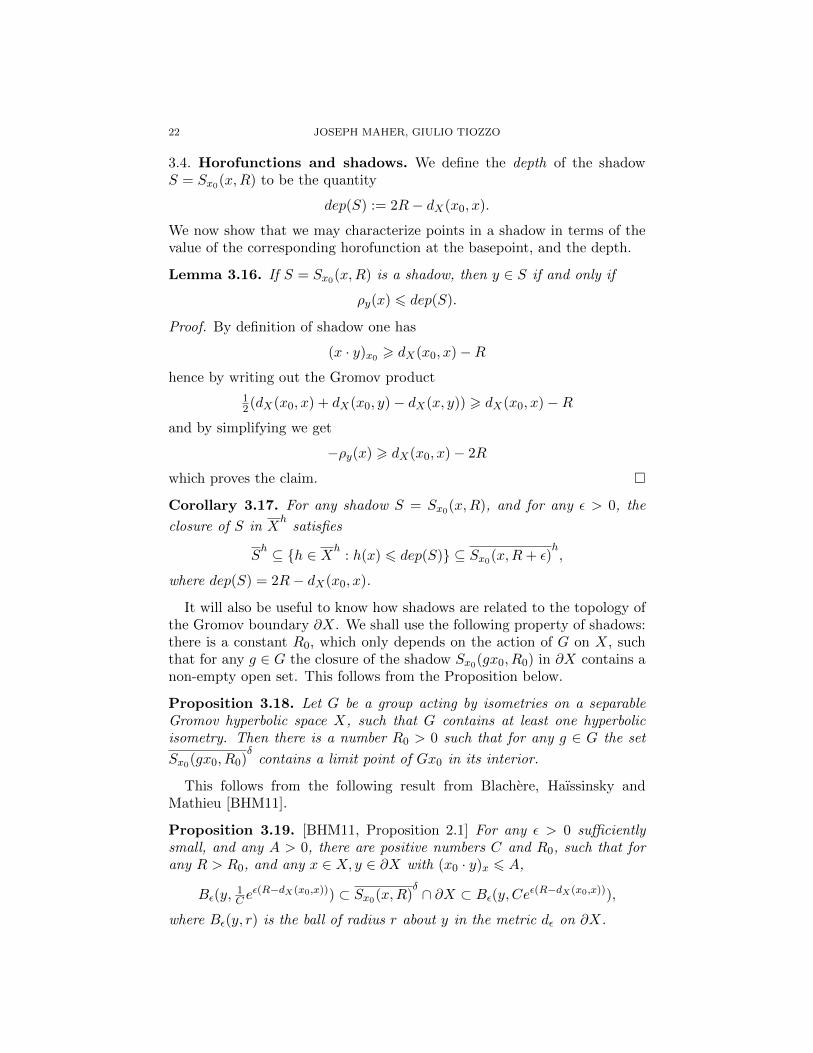
3.4. Horofunctions and shadows. We define the depth of the shadowS = Sx0(x,R) to be the quantity
dep(S) := 2R− dX(x0, x).
We now show that we may characterize points in a shadow in terms of thevalue of the corresponding horofunction at the basepoint, and the depth.
Lemma 3.16. If S = Sx0(x,R) is a shadow, then y ∈ S if and only if
ρy(x) 6 dep(S).
Proof. By definition of shadow one has
(x · y)x0 > dX(x0, x)−R
hence by writing out the Gromov product
12(dX(x0, x) + dX(x0, y)− dX(x, y)) > dX(x0, x)−R
and by simplifying we get
−ρy(x) > dX(x0, x)− 2R
which proves the claim.
Corollary 3.17. For any shadow S = Sx0(x,R), and for any ε > 0, the
closure of S in Xh
satisfies
Sh ⊆ h ∈ Xh
: h(x) 6 dep(S) ⊆ Sx0(x,R+ ε)h,
where dep(S) = 2R− dX(x0, x).
It will also be useful to know how shadows are related to the topology ofthe Gromov boundary ∂X. We shall use the following property of shadows:there is a constant R0, which only depends on the action of G on X, suchthat for any g ∈ G the closure of the shadow Sx0(gx0, R0) in ∂X contains anon-empty open set. This follows from the Proposition below.
Proposition 3.18. Let G be a group acting by isometries on a separableGromov hyperbolic space X, such that G contains at least one hyperbolicisometry. Then there is a number R0 > 0 such that for any g ∈ G the set
Sx0(gx0, R0)δ
contains a limit point of Gx0 in its interior.
This follows from the following result from Blachere, Haıssinsky andMathieu [BHM11].
Proposition 3.19. [BHM11, Proposition 2.1] For any ε > 0 sufficientlysmall, and any A > 0, there are positive numbers C and R0, such that forany R > R0, and any x ∈ X, y ∈ ∂X with (x0 · y)x 6 A,
Bε(y,1C e
ε(R−dX(x0,x))) ⊂ Sx0(x,R)δ ∩ ∂X ⊂ Bε(y, Ceε(R−dX(x0,x))),
where Bε(y, r) is the ball of radius r about y in the metric dε on ∂X.

RANDOM WALKS ON WEAKLY HYPERBOLIC GROUPS 23
Proof (of Proposition 3.18). Since G contains at least one hyperbolic isome-
try, then the limit set Gx0δ
contains at least two points in ∂X, which we callα+ and α−. Let α be a quasigeodesic from α+ to α−, and let p be a closestpoint on α to the basepoint x0. Given a group element g ∈ G, consider thetranslate gα, as illustrated in Figure 3 below.
gα+
gα−
gα
∂X
x0
q
gx0
gp
Figure 3. The translate of the quasigeodesic α under g.
For any element g ∈ G, let q be a nearest point on gα to x0. Anyquasigeodesic from x0 to either gα+ or gα− passes within distance O(δ)of q, so gx0 lies within distance dX(x0, α) + O(δ) of at least one of thesequasigeodesics, which we may assume has endpoint α+, up to relabeling.
Therefore, the product (x0 · gα+)gx0 is bounded above independently ofg ∈ G, hence by Proposition 3.19, there is a number R0, (depending only
on δ and the choice of α) such that the closure Sx0(gx0, R)δ ∩ ∂X contains
an open set containing gα+ ∈ Gx0δ, for any R > R0, as required.
3.5. Horofunctions and weak convexity of shadows. A priori, shad-ows need not be convex, or even quasi-convex. However, we now showvarious results about horofunctions and nested shadows which we can thinkof as weak versions of convexity. For example, for any two points con-tained in a shadow Sx0(x,R), the geodesic connecting them is contained inSx0(x,R+O(δ)). We start by showing that the value of a horofunction alonga geodesic is bounded by its values on the endpoints, up to an additive errorof O(δ).
Lemma 3.20. Let X a δ-hyperbolic, geodesic metric space. Then thereexists a constant C > 0, which depends only on δ, such that given anygeodesic segment [z1, z2] in X, with z1, z2 ∈ X, the following holds:
(13) minρz1(x), ρz2(x) − C 6 ρy(x) 6 maxρz1(x), ρz2(x)+ C
for any y ∈ [z1, z2] and any x ∈ X.

24 JOSEPH MAHER, GIULIO TIOZZO
Proof. Let us first assume that x, x0 belong to [z1, z2]. Up to swapping z1
and z2, we can assume x ∈ [z1, x0]; then we have the bound
ρz1(x) = −dX(x, x0) 6 ρy(x) = dX(x, y)− dX(x0, y) 6 dX(x, x0) = ρz2(x)
which yields the claim. Now, in the general case let px be the closest pointprojection of x to [z1, z2], and px0 the projection of x0. By the definition ofρz,
ρz(x) = dX(x, z)− dX(x0, z).
Then by the reverse triangle inequality (Proposition 2.2) we have for eachz ∈ X,
ρz(x) = dX(x, px) + dX(px, z)− dX(x0, px0)− dX(px0 , z) +O(δ),
hence for each i = 1, 2
ρy(x)− ρzi(x) = ρy(px)− ρzi(px) +O(δ),
where ρz(x) := dX(x, z)− dX(px0 , z) denotes the horofunction based at px0 .Since now px0 and px lie on [z1, z2], the claim follows by the previous case,and furthermore we may assume that the constant is positive.
Lemma 3.20 implies the following weak convexity property of both shad-ows and their complements.
Corollary 3.21. There exists a constant C > 0, which depends only on δ,such that for each shadow S = Sx0(x,R) the following hold:
(1) if z1 and z2 belong to S, then the geodesic segment [z1, z2] lies inSx0(x,R+ C);
(2) if z1 and z2 do not belong to S, then the geodesic segment [z1, z2]does not intersect Sx0(x,R− C).
Moreover, for each (Q, c) which satisfy Proposition 2.1, the above statementsstill hold with “geodesic” replaced by “(Q, c)-quasi-geodesic”, where this timeC depends on δ,Q, and c.
Proof. If z1, z2 belong to S, then ρzi(x) 6 dep(S) for each i = 1, 2 by Lemma3.16, hence Lemma 3.20 implies
ρy(x) 6 maxρz1(x), ρz2(x)+ C 6 dep(S) + C = dep(S′)
where S′ = Sx0(x,R + C/2), thus y ∈ S′ once again by Lemma 3.16. Theproof of (2) is similar, using the left-hand side of equation (13). The ex-tension to quasi-geodesic is immediate by the fellow-traveling property ofProposition 2.1.

RANDOM WALKS ON WEAKLY HYPERBOLIC GROUPS 25
4. Convergence to the boundary
In this section we prove the following theorem.
Theorem 4.1. Let G be a countable group of isometries of a geodesic, sep-arable, δ-hyperbolic space X (not necessarily proper), and let µ be a non-elementary probability measure on G. Then for each x0 ∈ X, almost everysample path (wnx0)n∈N converges in X∪∂X to a point of the Gromov bound-ary ∂X.
The proof of the theorem takes several steps, and it exploits the action ofG on the space of probability measures both on the horofunction compacti-
fication Xh
and on the Gromov boundary ∂X. The strategy of the proof isthe following:
(1) By compactness, there is a stationary measure ν on Xh
(Lemma4.3).
(2) The measure ν does not charge the finite part of the boundary:
ν(Xh∞) = 1 (Proposition 4.4).
(3) By the martingale convergence theorem (Proposition 4.13), for al-most every sample path the sequence of measures (wnν)n∈N con-
verges to some measure νω in P(Xh).
(4) By pushing the sequence forward to ∂X, using the local minimummap φ, almost every sequence (wnν)n∈N converges to some measureφ∗νω in P(∂X) (Lemma 4.14).
(5) Almost every sample path (wnx0)n∈N has a subsequence which con-verges to a point λ in the Gromov boundary ∂X (Proposition 4.7).
(6) Thus, by Lemma 4.15, almost every sample path (wn)n∈N has asubsequence (wnk
)k∈N such that (wnkν)k∈N converges to a delta-
measure δλ, for some λ ∈ ∂X.(7) Since the limit exists, almost every sequence (wnν)n∈N converges to
a delta-measure δλ (Proposition 4.16).(8) We prove that the fact that (wnν)n∈N converges to δλ implies that
the sample path (wnx0)n∈N converges to λ ∈ ∂X (Proposition 4.18).
In the rest of the section we shall work out the details of the proof.We remark that sample paths do not in general converge to points in the
horofunction compactification.
Example 4.2. Consider the nearest neighbour random walk on the Cayleygraph of F2 × Z/2Z, with respect to the standard generating set 〈a, b, c |[a, c], [b, c], c2〉, and with basepoint x0 corresponding to the identity element.If g ∈ F2, then ρg(c) = 1, and ρgc(c) = −1. As almost every sample path wn
hits each coset of F2 infinitely often, sample paths do not converge in Xh,
almost surely.
4.1. Random walks. We briefly review some background material on ran-dom walks and fix notation. Let µ be a probability distribution on G; the

26 JOSEPH MAHER, GIULIO TIOZZO
step space of the random walk generated by µ is the measure space (GZ, µZ),which is the countable infinite product of the measure spaces (G,µ). Eachelement of GZ is a sequence (gn)n∈Z, whose entries are the increments ofour (bi-infinite) random walk. The shift map T : GZ → GZ sends (gn)n∈Z to(gn−1)n∈Z, and is measure preserving and ergodic.
We define the location of the random walk at time n, which we shalldenote wn to be
wn =
g−10 g−1−1 . . . g
−1n+1 if n 6 −1
1 if n = 0g1g2 . . . gn if n > 1.
This gives a map GZ → GZ, defined by (gn)n∈Z 7→ (wn)n∈Z . We shalldenote the range of the location map as Ω, to distinguish it from the stepspace, and call P the pushforward to Ω of the product measure µZ on thestep space GZ. We shall refer to (Ω,P) as the path space, and elementsω ∈ Ω as sample paths of the random walk. The shift map T acts on Ω byT k : (wn)n∈Z 7→ (w−1
k wn+k)n∈Z, and is measure preserving and ergodic.
4.2. Stationary measures. Let M be a metrizable topological space, anddenote P(M) the space of Borel probability measures on M . The spaceP(M) is endowed with the weak-* topology, which is defined by sayingνn → ν if for each continuous bounded function f on M one has νn(f) →ν(f).
If now G is a countable group which acts on M by homeomorphisms, wedenote gν the pushforward of ν ∈ P(M) under the action of g ∈ G, i.e.gν(U) = ν(g−1U), and define the convolution operator ? : P(G)× P(M)→P(M) as the average of the pushforwards:
µ ? ν :=∑g∈G
µ(g) gν.
We say that a probability distribution ν on M is µ-stationary if µ ? ν = ν,i.e. for each Borel set U we have
(14) ν(U) =∑g∈G
µ(g)ν(g−1U).
A space M equipped with a µ-stationary measure ν is called a (G,µ)-space.Now, if we fix a base point x0 ∈ M , we shall write µ ∈ P(M) for thepushforward of µ under the orbit map, i.e. if U ⊂ M then µ(U) = µ(g ∈G : gx0 ∈ U). We shall write µn for the n-fold convolution of µ withitself on G, we shall write µn for the pushforward of µn to M , and finally,we shall write µn for the Cesaro averages of the pushforward measures,µn := 1
n(µ + µ2 + · · · + µn). Classical compactness arguments yield thefollowing:
Lemma 4.3. Let G be a countable group which acts by homeomorphismson a compact metric space M , and let µ be a probability distribution on G.Then there exists a µ-stationary Borel probability measure ν on M .

RANDOM WALKS ON WEAKLY HYPERBOLIC GROUPS 27
Proof. Since M is a compact metrizable space, then P(M) is compact inthe weak-∗ topology. Then any weak-∗ limit point of the sequence (µn)n∈Nof the Cesaro averages is µ-stationary. An alternate proof follows from theSchauder-Tychonoff fixed point theorem.
Applying the above arguments toXh
implies that there exists a µ-stationary
measure ν on Xh, i.e. (X
h, ν) is a (G,µ)-space. We now show that the mea-
sure ν is supported on Xh∞.
Proposition 4.4. Let G be a countable group of isometries of a separableGromov hyperbolic space X. Let µ be a non-elementary probability distribu-
tion on G, and let ν be a µ-stationary measure on Xh. Then
ν(XhF ) = 0.
In order to show that some set Y has measure zero, the basic idea is toconsider the translates gY of the set Y , and to consider the supremum ofthe measures of these sets. If we choose a translate gY with measure veryclose to the supremum, then by µ-stationarity, if hgY is another translatewith µ(h) > 0, then ν(hgY ) will also be close to the supremum. If there areenough disjoint translates with ν-measures close to the supremum, then thetotal measure of ν is strictly greater than one, which contradicts the factthat ν is a probability measure. We now make this precise.
Lemma 4.5. Let G be a countable group acting by homeomorphisms on ametric space M , let µ be a probability distribution on G, and let ν be a µ-stationary probability measure on M . Moreover, let us suppose that Y ⊂Mhas the property that there is a sequence of positive numbers (εn)n∈N suchthat for any translate fY of Y there is a sequence (gn)n∈N of group elements(which may depend on f), such that the translates fY, g−1
1 fY, g−12 fY, . . . are
all disjoint, and for each gn, there is an m > 1, such that µm(gn) > εn.Then ν(Y ) = 0.
The proof of this is a variation on [Mah10b, Lemma 3.5], but we providea proof for the convenience of the reader.
Proof. Suppose that s := supν(fY ) : f ∈ G > 0. Choose N > 2/s, letε = minεi : 1 6 i 6 N, and let εs = ε/N . Finally, choose f such that theharmonic measure of fY is within εs of the supremum, i.e. ν(fY ) > s− εs.By hypothesis, there is a sequence of group elements g1, . . . , gN such thatthe N translates g−1
1 fY, . . . , g−1N fY , are all disjoint, and for each gn there is
an m such that with µm(gn) > ε.The harmonic measure ν is µ-stationary, and hence µm-stationary for any
m, which implies
ν(fY ) =∑h∈G
µm(h)ν(h−1fY ).

28 JOSEPH MAHER, GIULIO TIOZZO
For any element g ∈ G we may rewrite this as
µm(g)ν(g−1fY ) = ν(fY )−∑h∈G\g
µm(h)ν(h−1fY ).
As we have chosen fY to have measure within εs of the supremum, thisimplies
µm(g)ν(g−1fY ) > s− εs −∑h∈G\g
µm(h)ν(h−1fY ).
The harmonic measure of each translate of Y is at most the supremum s,
µm(g)ν(g−1fY ) > s− εs − s∑h∈G\g
µm(h),
and the sum of µm(h) over all h ∈ G \ g is equal to 1−µm(g), which impliesthat
µm(g)ν(g−1fY ) > s− εs − s(1− µm(g)).
Let us now suppose g = gn for some n. By hypothesis, there is an m > 1such that µm(g) > 0. For such an m we may divide by µm(g) to give thefollowing estimate for the harmonic measure of the translate,
ν(g−1fY ) > s− εs/µm(g).
By assumption, such an estimate holds for each of the N disjoint translatesg−1i fY , and furthermore, µm(gi) > ε for each i. This implies that
ν(N⋃i=1
g−1i fY ) = ν(g−1
1 fY ) + · · ·+ ν(g−1N fY ) > N(s− εs/ε).
As we chose N > 2/s, and εs/ε = 1/N , this implies that the total measureν(⋃g−1i fY ) is greater than one, a contradiction.
We now complete the proof of Proposition 4.4. Recall that the translationlength τ(g) of an isometry g of X is defined to be
τ(g) := limn→∞
1ndX(x0, g
nx0).
This definition is independent of the base point x0, and τ(g) > 0 if and onlyif g is a hyperbolic isometry, and furthermore τ(gk) = kτ(g).
Proof of Proposition 4.4. We shall apply Lemma 4.5 taking as Y the set ofhorofunctions whose local minimum lies in a given ball around the base-
point: precisely, Y = h ∈ XhF : φ(h) ∩ B(x0, r) 6= ∅, where φ is the
local minimum map, and B(x0, r) is a ball of radius r in X. As µ is non-elementary, the semigroup generated by the support of µ contains hyperbolicisometries of arbitrarily large translation length. Choose such a hyperbolicisometry g with translation length τ(g) greater than 2r+K, where K is the

RANDOM WALKS ON WEAKLY HYPERBOLIC GROUPS 29
bound on the diameter of φ(h) from Lemma 3.13. Now, for any f ∈ G, thetranslates g−nfB(x0, r) are all at least distance τ(g)− 2r > K apart, henceno φ(h) can intersect two of them, so the sets g−nfY are all disjoint. As glies in the semigroup generated by the support of µ, for each n > 1 there isan m > 1 such that µm(gn) > 0. Set εn = µm(gn), for some such m, thenLemma 4.5 implies that ν(Y ) = 0. As this holds for every r, this implies
that ν(XhF ) = 0, as required.
The measure ν is therefore supported on Xh∞, and as φ is continuous on
Xh∞, the measure ν pushes forward to a Borel probability measure
ν := φ∗ν
on the Gromov boundary ∂X. The measure ν is a µ-stationary probabilitymeasure on ∂X, so (∂X, ν) is a (G,µ)-space. We now show that ν is non-atomic, which implies that ν is non-atomic as well. Recall that if the actionof G on X is non-elementary, then G does not preserve any finite subset ofthe boundary ∂X.
Lemma 4.6. Let G be a countable group which acts by isometries on a sep-arable Gromov hyperbolic space X. Let µ be a non-elementary probability
distribution on G, and let ν be a µ-stationary measure on Xh, with push-
forward ν on ∂X under the local minimum map φ. Then the measure ν isnon-atomic (hence so is ν). Furthermore, any µ-stationary measure on ∂X
is the pushforward of a µ-stationary measure on Xh∞.
Proof. Let Γ denote the group generated by the support of µ. We firstobserve that if there are atoms, then there must be an atom of maximalweight, as an infinite sequence of atoms (bn)n∈N of increasing weights hastotal measure greater than one. Let m be the maximal weight of any atom,and let Am be the collection of atoms of weight m, which is a finite set. Asν is µ-stationary, if b ∈ Am, then
ν(b) =∑g∈G
µ(g)ν(g−1b).
As no atom has weight greater than m, all elements of the orbit of b under Γmust have the same weight m, so Am is a finite, Γ-invariant set, contradictingthe fact that µ is non-elementary.
Finally, as the local minimum map φ : Xh∞ → ∂X is surjective, the push-
forward map φ∗ : P(Xh∞) → P(∂X) is also surjective, see e.g. [AB06, The-
orem 15.14]. If λ is a µ-stationary measure on ∂X, then φ−1∗ (λ) is a non-
empty, convex subspace of the space of measures on Xh∞, which can also be
seen as a subspace of the space P(Xh) of probability measures on X
h. Thus,
the closure H of φ−1∗ (λ) in P(X
h) is compact, convex, and invariant under
convolution with µ, so by the Schauder-Tychonoff fixed point theorem there
is a µ-stationary measure ν in H ⊆ P(Xh). However, by Proposition 4.4, ν

30 JOSEPH MAHER, GIULIO TIOZZO
vanishes on the set of finite horofunctions, hence it belongs to P(Xh∞), and
since ν is a limit of elements in φ−1∗ (λ) and φ∗ is continuous, we also have
φ∗ν = λ, as required.
4.3. Convergent subsequences. The goal of this section is to prove thefollowing step in the proof of Theorem 4.1:
Proposition 4.7. Let G be a countable group of isometries of a separa-ble Gromov hyperbolic space X, and let µ be a non-elementary probabilitydistribution on G.
Then, for P-almost every sample path (wn)n∈N there is a subsequence of
(ρwnx0)n∈N which converges to a horofunction in Xh∞.
As a corollary, P-almost every sample path (wn)n∈N has a subsequence(wnk
)k∈N such that (wnkx0)k∈N converges to a point in the Gromov boundary
∂X.
Given a shadow S = Sx0(x,R), we define the open shadow S = Sx0(x,R)
to be the subset of Xh
given by
Sx0(x,R) := h ∈ Xh: h(x) < dep(S).
As x is compact and (−∞, dep(S)) is open in R, the set S is an open
subset of Xh
contained in the interior of Sh.
Lemma 4.8. For each T < 0, the set Xh∞ is contained in a countable
collection of open shadows of depth 6 T .
Proof. We have immediately from the definition
Xh∞ ⊆ h ∈ X
h | inf h < T =⋃x∈Xh ∈ Xh | h(x) < T.
Now, by picking a countable dense subset xii∈N of X and an enumerationTjj∈N of (−∞, T ) ∩Q, we have
Xh∞ ⊆
⋃i,j∈Nh | h(xi) < Tj,
as required.
We shall now define a descending shadow sequence to be a sequence S =(SM )M∈N, where each SM is a finite collection of shadows, and each shadowS ∈ SM has depth dep(S) 6 −M .
Given a descending shadow sequence S, we shall introduce (for conve-nience of notation) an indexing of all its shadows, i.e.
⋃M SM = S1, S2, . . . .
We say a M -tuple I = (i1, . . . , iM ) of positive integers is an index set of depthM for S if each j = 1, . . . ,M , the shadow Sij is an element of Sj (hence,it has depth 6 −j). Given a descending shadow sequence S, and an index

RANDOM WALKS ON WEAKLY HYPERBOLIC GROUPS 31
set I = (i1, . . . , iM ), we define the cylinder CI to be the intersection of theopen shadows Sij corresponding to the indexed shadows Sij , i.e.
CI := Si1 ∩ · · · ∩ SiM,
so CI is an open set in Xh. Given a number M ∈ N, let ΣM be
ΣM :=⋃
I index setof depth M
CI =⋃Si1 ∩ · · · ∩ S
iM,
where the union is taken over all index sets of depth M . The sets ΣM form
a nested sequence of open sets in Xh, i.e.
Σ1 ⊇ Σ2 ⊇ Σ3 ⊇ · · · .Finally, we observe that by Lemma 3.16, if h ∈ ΣM then inf h 6 −M , so⋂
M∈NΣM ⊆ X
h∞.
Lemma 4.9. Let (yn)n∈N be a sequence of points of X, and let (SM )M∈Nbe a descending shadow sequence. If (ρyn)n∈N intersects ΣM for each M ,then there exists a subsequence (ynk
)k∈N such that (ρynk)k∈N converges to a
horofunction in Xh∞.
Proof. Suppose the sequence (ρyn)n∈N intersects each ΣM . So for each M ∈N there is an nM such that ρynM
∈ ΣM . As⋂
ΣM ⊂ Xh∞, each ρyn may lie
in only finitely many ΣM , and so nM → ∞ as M → ∞. The horofunctionρynk
lies in Σk, which is a union of cylinders, so there is an index set Ik =
(i1, . . . , ik) of depth k such that
ρynk∈ CIk = Si1 ∩ · · · ∩ S
ik.
Recall that, by definition of descending shadow sequence and index set,there are only finitely many choices for the first entry i1 in each index setIk, so we may pass to a further subsequence in which i1 is constant. Choosen1 to be the first element of this subsequence, and relabel the remainingelements as (nk)k∈N for k > 2. Again, as there are only finitely manychoices for the second entry i2 in the index set Ik, we may pass to a furthersubsequence in which the indices i2 are constant for all k > 2. Continuing bya standard diagonal procedure, we may construct a subsequence (ynk
)k∈N,and a sequence of indices (ik)k∈N, such that
ρynk∈ Si1 ∩ · · · ∩ S
ik,
for each k.By compactness, the sequence (ρynk
)k∈N has a limit point h ∈ Xh. Then
by Lemma 3.16, for each j and each k > j, if Sij = Sx0(xj , Rj), we have
ynk∈ Sij , hence
ρynk(xj) 6 −j,

32 JOSEPH MAHER, GIULIO TIOZZO
thus by passing to the limit as k →∞ we have
h(xj) 6 −j for all j > 1,
which gives h ∈ Xh∞.
Lemma 4.10. Let ε > 0, and let ν be a µ-stationary measure on Xh. Then
there exists a finite descending shadow sequence S = (SM )M∈N such that foreach M ,
ν(ΣM ) > 1− ε.
Proof. Recall by Lemma 4.8 that for any M ∈ N there exists a countable
collection of shadows of depth 6 −M which covers Xh∞, and X
h∞ has full
measure by Proposition 4.4. Thus, since probabilities are countably additiveone can find a finite set SM := SM,1, . . . , SM,rM of shadows of depth6 −Msuch that the union SM :=
⋃rMi=1 SM,i satisfies
ν(SM ) > 1− 2−M ε.
We may now set S to be the sequence (SM )M∈N, which is a descendingshadow sequence. We now observe that ν(ΣM ) ≥ 1−ε/2−· · ·−ε/2M > 1−εas required.
We may now complete the proof of Proposition 4.7.
Proof (of Proposition 4.7). We shall show that the set Z of sequences (wn)n∈Nin the path space (Ω,P) for which (ρwn)n∈N does not have limit points in
Xh∞ has measure at most ε, for each ε > 0. Fix ε > 0, and let (SM )M∈N
be a descending shadow sequence constructed according to Lemma 4.10, us-ing a measure ν which is a µ-stationary weak limit of the Cesaro averagesµn = 1
n(µ1 + · · ·+ µn). Now, suppose that the sequence (ρwn)n∈N does not
have limit points in Xh∞: then by Lemma 4.9 there exists an index M such
that ρwn does not belong to ΣM for any n. Thus we have the inclusion
Z ⊆⋃M
⋂n
(wk)k∈N : ρwn /∈ ΣM,
so if we set YM := Xh \ ΣM , then
P(Z) 6 supM
infnµn(YM ).
Then, by definition of the Cesaro averages, inf µn(YM ) > inf µn(YM ), so thisimplies that
P(Z) 6 supM
infnµn(YM ).
Furthermore as ν is a weak limit point of the Cesaro averages µn, and YMis closed, we have for each M ,
infnµn(YM ) 6 ν(YM ),

RANDOM WALKS ON WEAKLY HYPERBOLIC GROUPS 33
hence by Lemma 4.10
P(Z) 6 supM
ν(YM ) 6 ε,
and the claim is proven. The corollary follows from Proposition 3.14.
4.4. The boundary action. We now prove Theorem 1.1, convergence tothe boundary. We start by showing that the action of G on X ∪∂X satisfies
the following property (which need not hold for the action of G on Xh):
if the sequence (gnx0)n∈N converges to a point in ∂X, then the sequence(gny)n∈N converges to the same point, for any y ∈ X.
Lemma 4.11. Let X be a Gromov hyperbolic space. If x0 ∈ X and thesequence (gnx0)n∈N converges to a point λ in ∂X, then the sequence (gny)n∈Nconverges to the same point λ, for any y ∈ X.
Proof. Consider the Gromov product
(gnx0 · gny)x0 = 12(dX(x0, gnx0) + dX(x0, gny)− dX(gnx0, gny)).
By the triangle inequality dX(x0, gny) > dX(x0, gnx0)− dX(gnx0, gny), andas gn is an isometry, dX(gnx0, gny) = dX(x0, y). This implies
(gnx0 · gny)x0 > dX(x0, gnx0)− dX(x0, y),
which tends to infinity as n tends to infinity, so (gny)n∈N converges to thesame limit point as (gnx0)n∈N.
The following is a version of Kaimanovich [Kai00, Lemma 2.2] in thenon-proper case.
Lemma 4.12. Let G be a group of isometries of a Gromov hyperbolic spaceX. Let (gn)n∈N be a sequence in G such that (gnx0)n∈N → λ ∈ ∂X. Thenthere is a subsequence (gnk
)k∈N such that (gnkx)k∈N → λ for all but at most
one point of X ∪ ∂X.
Proof. We show that there is a subsequence (gnk)k∈N for which there is at
most one point b ∈ ∂X such that (gnkb)k∈N 6→ λ. Suppose there is a point
b1 in ∂X such that (gnb1)n∈N 6→ λ. This implies there is an open set U1
in X ∪ ∂X containing λ such that infinitely many gnb1 do not lie in U1.Therefore, we may pass to a subsequence (gnk
)k∈N such that gnkb1 6∈ U1 for
all k. Now suppose there is another point b2 ∈ ∂X such that (gnkb2)k∈N 6→
λ. This implies there is an open set U2 containing λ such that infinitelymany gnk
b2 do not lie in U2. As before, we may pass to a subsequence,which by abuse of notation we shall continue to call (gnk
)k∈N , such that(gnk
b2)k∈N 6∈ U2 for all n. As U1 ∩U2 is also an open neighbourhood of λ, it
contains a shadow set of the form S1 = Sx0(x,R)δ, with λ contained in the
interior of the slightly smaller shadow S2 = Sx0(x,R− C)δ, where C will
be chosen as the weak convexity constant of Corollary 3.21 for (Q, c)-quasi-geodesics. Let now γ be a (Q, c)-quasigeodesic from b1 to b2, and y ∈ X apoint on γ. By Corollary 3.21, since the endpoints gnk
b1 and gnkb2 do not

34 JOSEPH MAHER, GIULIO TIOZZO
belong to S1, then the point gnky does not belong to S2. However, this is
a contradiction, as by Lemma 4.11 we know that gnky → λ, hence it must
eventually lie inside S2.
4.5. Convergence of measures. We will use the following result, whichgoes back to Furstenberg [Fur63, Corollary 3.1], see also Margulis [Mar91,Chapter VI].
Proposition 4.13. Let M be a compact metric space on which the countablegroup G acts continuously, and ν a µ-stationary Borel probability measureon M . Then for P-almost all sequences (wn)n∈N the limit
νω := limn→∞
g1g2 . . . gnν
exists in the space P(M) of probability measures on M .
To give a brief overview of the argument, one proves that, since the mea-sure is stationary, for each continuous function f ∈ C(M) the process
Xn :=
∫Xf(g1 . . . gnx) dν(x)
is a bounded martingale, hence converges almost surely; this defines a pos-itive linear functional on the space C(M), which is thus represented by aBorel measure.
Furthermore, if wnν → νω a.s., then we get the integral formula
(15) ν =
∫Ωνω dP(ω).
Lemma 4.14. Let G be a countable group of isometries of a separable Gro-mov hyperbolic space X, let µ be a non-elementary probability distributionon G, and let ν be a µ-stationary Borel measure on ∂X.
Then for almost every sample path ω = (wn)n∈N, the sequence of measures(wnν)n∈N converges to a measure νω ∈ P(∂X).
Proof. By Lemma 4.6, there is a µ-stationary probability measure ν on Xh∞
such that ν is the pushforward of ν. Applying Proposition 4.13 to the action
of G on Xh, the sequence (wnν)n∈N converges to a measure νω ∈ P(X
h),
almost surely. Moreover, since ν vanishes on XhF and X
hF is G-invariant, the
measures wnν also vanish on XhF for each wn; furthermore, by equation (15)
the limit νω also vanishes on XhF for almost every ω. Now, note that X
h∞
is a countable intersection of open subsets of Xh, hence it is a Borel subset
of Xh, so the weak-∗ topology on P(X
h∞) (arising from Cb(X
h∞)) is the
relativization of the weak-∗ topology on P(Xh), see e.g. [AB06, Theorem
15.4]. Since wnν → νω a.s. in P(Xh) and both wnν and νω belong to
P(Xh∞), this implies that a.s. wnν → νω in the weak-∗ topology of P(X
h∞).
Finally, since φ is continuous, the pushforward map P(Xh∞) → P(∂X) is
continuous, hence wnν = φ∗wnν → φ∗νω = νω as claimed.

RANDOM WALKS ON WEAKLY HYPERBOLIC GROUPS 35
We wish to show that for P-almost all sequences (wn)n∈N, the measureνω is a δ-measure, and as the limit exists, it suffices to show this for anysubsequence (wnk
)k∈N. We have already shown, by Proposition 4.7, thatalmost every sequence (wn)n∈N in (Ω,P) has a subsequence (wnk
)k∈N suchthat (wnk
x0)k∈N converges to a point in ∂X, so it suffices to show that ifa sequence (gn)n∈N has the property that (gnx0)n∈N converges to λ ∈ ∂X,then the measures (gnν)n∈N converge to δλ.
Lemma 4.15. Let G be a non-elementary countable group of isometries ofa separable Gromov hyperbolic space X, and let (gn)n∈N be a sequence in Gsuch that gnx0 → λ ∈ ∂X. Then for any non-atomic probability measure νon ∂X there is a subsequence (gnk
)k∈N such that the translations (gnkν)k∈N
converge in the weak-∗ topology to a delta-measure δλ, supported on λ.
Proof. By Lemma 4.12, there exists a subsequence (nk)k∈N and a pointx ∈ ∂X such that for all b ∈ ∂X, b 6= x, one has gnk
b → λ. Since themeasure ν is non-atomic, ν(x) = 0 and the claim follows by the dominatedconvergence theorem.
Proposition 4.16. Let G be a countable group of isometries of a separableGromov hyperbolic space X, let µ be a non-elementary probability distribu-tion on G, and let ν be a µ-stationary probability measure on ∂X.
Then for almost every sample path ω = (wn)n∈N, there is a boundarypoint λ(ω) ∈ ∂X such that the sequence of measures (wnν)n∈N converges inP(∂X) to a delta-measure δλ(ω).
Proof. By Proposition 4.7, almost every sample path ω has a subsequencewhich converges to some point λ(ω) ∈ ∂X. Thus, by Lemma 4.15, thereexists a subsequence (wnk
)k∈N such that (wnkν)k∈N → δλ(ω). By Lemma
4.14, the sequence (wnν)n∈N has a limit, hence the limit must coincide withδλ(ω).
4.6. Convergence to the boundary: end of proof. We have shown thatP-almost every sequence (wnν)n∈N converges to a δ-measure on ∂X. Finally,we now show that this implies that P-almost every sequence (wnx0)n∈Nconverges to some point in the Gromov boundary ∂X.
We start by showing that there are two shadows with disjoint closuresand positive measure.
Lemma 4.17. Let X be a separable, Gromov hyperbolic space, and ν anon-atomic probability measure on ∂X. Then there exist two shadows S1,
S2 in X such that their closures Ui := Siδ
in ∂X are disjoint, and both havepositive ν-measure.
Proof. As ∂X is a separable metric space, the support of ν is a non-emptyclosed set, and, since ν is non-atomic, it contains at least two points λ1
and λ2. Now, for each λi we can choose a shadow Si in X such that λi is
contained in the interior of the closure Ui = Siδ, hence ν(Ui) > 0 for each

36 JOSEPH MAHER, GIULIO TIOZZO
i = 1, 2, and such that the distance parameter of each Si is much larger than(λ1 · λ2)x0 , so that U1 and U2 are disjoint.
The next proposition completes the proof of Theorem 4.1.
Proposition 4.18. Let G be a countable group of isometries of a separableGromov hyperbolic space X, let µ be a non-elementary probability distribu-tion on G, and let ν be a µ-stationary measure on ∂X.
Suppose that the sequence (wnν)n∈N converges to a delta-measure δλ on∂X, for some λ ∈ ∂X. Then (wnx0)n∈N converges to λ in X ∪ ∂X.
Proof. Let U1 = S1δ
and U2 = S2δ
as in Lemma 4.17, applied to the sta-tionary measure ν. Set ε = minν(U1), ν(U2); as U1 and U2 both havepositive ν-measure, ε is strictly greater than zero. As the sequence ofmeasures (wnν)n∈N converges to the delta-measure δλ, for any shadow set
V = Sx0(x,R)δ
containing λ in its interior, there is an N such that
wnν(V ) > 1− ε/2 for all n > N.
As wnν(wnU1) = ν(U1) > ε, the set wnU1 intersects V , hence wnS1 intersectsthe (slightly larger) shadow S0 = Sx0(x,R + O(δ)), and similarly wnS2
intersects S0. For each i = 1, 2, let us pick yi ∈ Si ∩ w−1n S0 and denote
xi = wnyi ∈ S0.By disjointness of U1 and U2, there exists a constant C such that
(y1 · y2)x0 6 C
for each y1 ∈ U1 and y2 ∈ U2. Moreover, since G acts by isometries, we get
(x1 · x2)wnx0 = (y1 · y2)x0 6 C
hence we can bound the distance from wnx0 to the geodesic [x1, x2] as
dX(wnx0, [x1, x2]) = (x1 · x2)wnx0 +O(δ) 6 C +O(δ);
note that the constant on the right-hand side depends only on U1, U2 andδ, and not on n.
As x1 and x2 both lie in S0, by weak convexity (Corollary 3.21), a geodesic[x1, x2] connecting them lies in a shadow Sx0(x,R + O(δ)), and as wnx0 isa bounded distance from [x1, x2], this implies that wnx0 lies in the slightlylarger shadow S+
0 = Sx0(x,R+ C +O(δ)), for all n > N .As this holds for all shadow sets V containing λ in their interiors, this
implies that (wnx0)n∈N converges to λ, as required.
Theorem 4.1 implies the convergence statement in Theorem 1.1, and soit remains to show that the hitting measure ν is the unique µ-stationarymeasure on ∂X, and the convolution measures (µn) converge weakly to ν.
By Proposition 4.16, for any µ-stationary measure ν on ∂X, for P-almostevery sample path ω, the sequence of measures (wnν)n∈N converges to δλ(ω),where λ(ω) is the limit point of the sample path (wnx0)n∈N, hence it only

RANDOM WALKS ON WEAKLY HYPERBOLIC GROUPS 37
depends on ω, not on ν. Thus, uniqueness follows from the integral formula(15). Furthermore,
µn =
∫Ωwnδx0 dP(ω).
We may take the limit as n tends to infinity, and by the integral formula(15), the distribution of the limit points is given by ν, so µn weakly convergesto ν.
5. Applications
In this section we use convergence to the boundary to show the resultson positive drift, sublinear tracking and translation length.
We will no longer use measures on the horofunction boundary, and so weshall from now on simply denote by ν the hitting measure on the Gromovboundary ∂X. Moreover, given S ⊆ X, the symbol S from now on willalways mean the closure of S in the space X ∪ ∂X.
5.1. Hitting measures of shadows. We start by showing that the mea-sure of a shadow tends to zero as the distance parameter of the shadow tendsto infinity. In order to simplify notation, we shall denote
Sh(x0, r) := Sx0(gx0, R) : g ∈ G, dX(x0, gx0)−R > rthe set of shadows based at x0, with centers on the orbit Gx0 and withdistance parameter > r.
Proposition 5.1. Let G be a countable group of isometries of a separableGromov hyperbolic space X. Let µ be a non-elementary probability distribu-tion on G, and let ν be the hitting measure on ∂X. Then we have
limr→∞
supS∈Sh(x0,r)
ν(S) = 0.
This result also holds for the reflected measures µn and ν determined byµ(g) = µ(g−1), as if µ satisfies the hypotheses of Proposition 5.1, then sodoes µ.
Proof. Propositions 3.18 and 3.19 show that a shadow centered at gx0 ofdistance parameter r is contained in a ball of radius Ce−εr in the metric dεon ∂X, where C is independent of r, and as ν is non-atomic. It thereforesuffices to show that for any non-atomic probability measure ν on a metricspace (M,d),
supx∈M
ν(B(x, r))→ 0 as r → 0.
Suppose not, then there is an ε > 0 and a sequence of metric balls B(xn, rn)with rn → 0 and ν(B(xn, rn)) > ε > 0, for all n. Consider
Un =⋃B(x, r) | r 6 1/n and ν(B(x, r)) > ε,
and let U =⋂Un. The Un form a nested decreasing family of sets, i.e.
Um ⊆ Un for all m > n, and furthermore, ν(Un) > ε for all n. This implies

38 JOSEPH MAHER, GIULIO TIOZZO
that ν(U) > ε, and so in particular U is non-empty. For any point x ∈ U ,ν(B(x, r)) > ε for all r > 0, and this contradicts the fact that ν is non-atomic.
If µ has bounded range in X then the argument from [Mah12, Lemma
2.10] shows that the ν- and µn-measures of a shadow Sx0(gx0, R) decayexponentially in the distance parameter, i.e. there are positive constants Kand c < 1 such that
(16) ν(Sx0(gx0, R)) 6 KcdX(x0,gx0)−R.
For U a subset of X, let H+x (U) denote the probability that a random
walk starting at x ever hits U in forward time, i.e.
H+x (U) := P(∃ n > 0 : wnx ∈ U).
Similarly, let H−x (U) be the probability that a random walk starting at xever hits U in reverse time, i.e. the probability that wnx lies in U for somen 6 0.
Proposition 5.2. Let G be a countable group which acts by isometries ona separable Gromov hyperbolic space X, and µ a non-elementary probabilitydistribution on G. Then
supS∈Sh(x0,r)
H+x0(S)→ 0 as r →∞.
This immediately implies the same result with H+x0 replaced by H−x0 , by
replacing µ with the reflected measure µ(g) = µ(g−1).
Proof. Suppose a sample path starting at x0 hits a shadow S1 = Sx0(x,R)with x = hx0 in forward time, at gx0 say. Let γ be a geodesic from x0 to x,and let p be a nearest point on γ to gx0, as illustrated below in Figure 4.
x0 x
gx0
p
y
q
S1 = Sx0(x,R)S2 = Sx0(x,R+A)
Figure 4. Nested shadows
Consider the shadow S2 = Sx0(x,R+A), for some fixed A > 0 which wewill choose later. The main idea is that if the random walk ever hits S1,

RANDOM WALKS ON WEAKLY HYPERBOLIC GROUPS 39
it will likely converge inside the closure of S2, and the probability of thathappening is small if the distance parameter of S2 is large.
To make the idea precise, let y be a point in the complement of S2, and letq be the nearest point projection of y to γ. By Proposition 2.4, p is withindistance O(δ) of S1, and q is within distance O(δ) of the complement of S2,so the distance between p and q is at least A+O(δ). Now using Proposition2.3, if A > O(δ), then the Gromov product satisfies
(x0 · y)gx0 = dX(gx0, p) + dX(p, q) +O(δ) > A+O(δ).
Therefore, the complement of S2 is contained in a shadow S3 = Sgx0(x0, R′)
(where R′ = dX(gx0, x0)−A+O(δ)) of distance parameter A+O(δ).Fix some positive ε < 1; then, since the measure of shadows tends to
zero as the distance parameter tends to infinity (Proposition 5.1), thereis a number A0 sufficiently large such that ν(S) 6 ε for all shadows S ∈Sh(x0, A0) with distance parameter larger than A0. As a consequence, if wechoose A such that A+O(δ) > A0 in the above construction, we have
ν(g−1S3) = ν(Sx0(g−1x0, R′)) 6 ε
hence, since we proved ∂X \ S2 ⊆ X \ S2 ⊆ S3,
(17) ν(g−1S2) > 1− ε.
Now, by the Markov property of the random walk, the conditional probabil-ity of ending up in S2 after hitting an element gx0 ∈ S1 at time k is givenby
P( limn→∞
wnx0 ∈ S2 | wk = g) = P( limn→∞
wnx0 ∈ g−1S2) = ν(g−1S2)
for each k and g, and such probability is large by equation (17). This impliesthe following lower bound on the probability of ending up in S2: if we denoteby Ak,g the event “wk = g and wkx0 /∈ S1 for 0 6 h 6 k − 1” we have
P( limn→∞
wnx0 ∈ S2) > P( limn→∞
wnx0 ∈ S2 and ∃ n : wnx0 ∈ S1) =
=∑k∈N
gx0∈S1
P(Ak,g)P( limn→∞
wnx0 ∈ S2 | wk = g) >
> P(∃ n : wnx0 ∈ S1)(1− ε)
which, by recalling the definitions of ν and H+x0 , becomes
(18) H+x0(S1) 6
1
1− εν(S2).
Now, as the distance parameter of S1 tends to ∞, so does the distanceparameter of S2, hence ν(S2) → 0 by Proposition 5.1, and by the aboveequation H+
x0(S1) tends to 0, as required.
As H+x0(S1) is an upper bound for µn(S1) for any n, equation (18) implies
the following corollary.
40 JOSEPH MAHER, GIULIO TIOZZO
Corollary 5.3. Let G be a countable group which acts by isometries on aseparable Gromov hyperbolic space X, and let µ be a non-elementary prob-ability distribution on G. Then there is a function f(r), with f(r) → 0 asr →∞ such that for all n one has
(19) supS∈Sh(x0,r)
µn(S) 6 f(r).
As the reflected random walk also satisfies the hypotheses of Corollary 5.3,we obtain a similar result for µn, though possibly for a different function f .
Proposition 5.4. Let G be a non-elementary, countable group acting byisometries on a separable Gromov hyperbolic space X, and let µ be a non-elementary probability distribution on G. Then there is a number R0 suchthat for any group elements g and h in the semigroup generated by the sup-port of µ, the closure of the shadow Shx0(gx0, R0) has positive hitting mea-sure for the random walk determined by µ.
Proof. Let us first assume h = 1. By Proposition 3.18, there is a constantR0 such that every shadow S1 = Sx0(gx0, R0) contains a limit point λ ofGx0 in the interior of its closure. We may now follow the same argument asin Proposition 5.2. Choose a shadow S2 = Sx0(gx0, R0) containing λ suchthat dX(S2, X \ S1) is at least A+O(δ) (note that here the roles of S1 andS2 are reversed with respect to Proposition 5.2, as S2 ⊆ S1). In particular,this implies that for any point y ∈ S2, the complement of S1 is containedin a shadow Sy(x0, R) with distance parameter at least A. By Proposition5.1 the measure of shadows tends to zero as the distance parameter tendsto infinity, so given a positive number ε < 1 we may choose A sufficientlylarge so that ν(S) 6 ε for all shadows S ∈ Sh(x0, A).
Let (gn)n∈N be a sequence in the semigroup generated by the support ofµ such that (gnx0)n∈N converges to λ. Let gn be an element of the sequencewith gnx0 ∈ S2, and let k be such that µk(gn) > 0. Now using the Markovproperty of the random walk, the conditional probability of converging tothe closure of S1, having hit S2, is at least 1− ε, and so
ν(S1) > (1− ε)µk(gn),
which is positive, as required. Now, the case h 6= 1 can be reduced to theprevious one; indeed, given h in the support of the random walk generatedby µ, there exists by hypothesis an n such that µn(h) > 0, which implies
ν(Shx0(gx0, R0)) > P(wn = h) P(limmwmx0 ∈ Shx0(gx0, R0) | wn = h)
which by the Markov property of the walk equals
µn(h) P(limmwmx0 ∈ Sx0(h−1gx0, R0))
and this is positive by the previous case.

RANDOM WALKS ON WEAKLY HYPERBOLIC GROUPS 41
5.2. Positive drift. In this section we prove Theorem 1.2, i.e. that thesample paths (wnx0)n∈N of the random walk have positive drift in X.
It will be convenient to consider the k-step random walk (wkn)n∈N, andintroduce the notation xi := wkix0 for each i. Let χki : Ω→ R be the randomvariable given by the distance in X traveled by the sample path from timek(i− 1) to time ki, i.e.
χki (ω) := dX(wk(i−1)x0, wkix0) = dX(xi−1, xi).
For fixed k, the χki are independent identically distributed random variableswith common distribution χk1.
Given a number R, we say a subsegment [xi, xi+1] of the sample path ispersistent if the following three conditions are satisfied:
dX(xi, xi+1) > 2R+ 2C + C0(20)
xn ∈ Sxi+1(xi, R) for all n 6 i(21)
xn ∈ Sxi(xi+1, R) for all n > i+ 1(22)
The constant C in (20) is the weak convexity constant from Corollary3.21, while C0 will only depend on δ and will be chosen later. A persistentsubsegment is illustrated in Figure 5 below.
xi
xi+1
Sxi(xi+1, R)Sxi+1(xi, R)
Figure 5. A persistent segment of the sample path.
Choose an ε, with 0 < ε < 13 . We now show that given such a choice of
ε, we may choose both R and k sufficiently large such that for any i each ofthe three conditions holds with probability at least 1− ε.
The probability that (21) holds is the same as the probability that wknx0
never hits the complement of the shadow Sxi+1(xi, R) for any n 6 i. As thecomplement of this shadow is contained in a shadow
Si = Sxi(xi+1, Ri)
where Ri = dX(xi, xi+1) − R + O(δ), the probability that (21) holds is atleast
1− P(∃ n 6 ki : wnx0 ∈ Si)

42 JOSEPH MAHER, GIULIO TIOZZO
which equals by the Markov property
(23) 1−H−x0(w−1ki Si).
The distance parameter of w−1ki Si, which equals the distance parameter of
Si, is R + O(δ); hence, by Proposition 5.2, we may choose R sufficientlylarge such that (23) is at least 1− ε.
A similar argument shows that the probability that (22) holds is at least
(24) 1−H+x0(w−1
k(i+1)Sxi+1(xi, Ri))
and again we may choose R sufficiently large such that (24) is at least 1− ε.Finally, the probability that (20) holds is P(χki > 2R+2C+C0) = P(χk1 >
2R + 2C + C0), since χki and χk1 have the same law. We have shown thatalmost every sample path converges to a point in the Gromov boundary, soin particular, sample paths are transient on bounded sets. This implies thatfor any R and ε, there is a sufficiently large k, depending on R and ε, suchthat
P(χk1 6 2R+ 2C + C0) < ε
as required. Therefore, for the choice of ε, R and k described above, theprobability that each condition holds individually is at least 1 − ε. Thethree conditions need not be independent, but the probability that all threehold simultaneously is at least η := 1− 3ε, which is positive as ε < 1
3 .
Thus, if we define for each i the random variable Y ki : Ω→ R
Y ki (ω) :=
1 if [xi, xi+1] is persistent0 otherwise.
we get that the Y ki are identically distributed (but not independent), with
finite expectation since they are bounded; moreover, for each i
(25) E(Y ki ) > η > 0.
We now show that the number of persistent segments lying between x0
and wknx0 gives a lower bound on the distance dX(x0, wknx0).Let γ be a geodesic from x0 to xn = wknx0, and suppose that [xi, xi+1] is a
persistent subsegment of the sample path. By (21), x0 lies in Sxi+1(xi, R) fori > 0, and by (22), xn lies in Sxi(xi+1, R) for n > i+ 1. As the two shadowsare at least distance 2C+C0−O(δ) apart, the geodesic γ has a subsegment γiof length at least C0−O(δ) > C0/2 which fellow travels with [xi, xi+1], andwhich is disjoint from both Sxi+1(xi, R+ C) and Sxi(xi+1, R+ C). Now let[xj , xj+1] be a different persistent subsegment. The same argument as aboveshows that there is a subsegment γj of γ of length at least C0/2 which fellowtravels with [xj , xj+1]. We now show that γi and γj are disjoint subsegmentsof γ. Up to relabeling, we may assume that i < j. Then both xj and xj+1
lie in Sxi(xi+1, R), and so by weak convexity, Corollary 3.21, any geodesicconnecting them lies in Sxi(xi+1, R+C), and so in particular γi and γj aredisjoint subsegments of γ. Therefore the distance dX(x0, wknx0) is at leastC0/2 times the number of persistent subsegments between x0 and wknx0.

RANDOM WALKS ON WEAKLY HYPERBOLIC GROUPS 43
We will now apply Kingman’s subadditive ergodic theorem, [Kin68], usingthe following version from [Woe00, Theorem 8.10]:
Theorem 5.5. Let (Ω,P) be a probability space and U : Ω → Ω a measurepreserving transformation. If Wn is a subadditive sequence of non-negativereal-valued random variables on Ω, that is, Wn+m 6 Wn + Wm Un forall m,n ∈ N, and W1 has finite first moment, then there is a U -invariantrandom variable W∞ such that
limn→∞
1nWn = W∞
P-almost surely, and in L1(Ω,P).
In order to apply the theorem, let us define for each n the variable
Zkn :=n−1∑i=0
Y ki = #0 6 i 6 n− 1 : [xi, xi+1] is persistent
which gives the number of persistent subsegments along a given sample pathfrom x0 to xn = wknx0. The random variables (Zkn)n∈N are non-negativeand have finite expectation, since Zkn 6 n for each n, and the sequence issubadditive by the Markov property. Moreover, as expectation is additive,we get from equation (25)
E(Zkn) =n−1∑i=0
E(Y ki ) > nη
with η > 0. We now apply Theorem 5.5 taking as Ω the step space of thekth-step random walk, U the shift map, and the Zkn as random variables (forfixed k); we get that the sequence ( 1
nZkn)n∈N converges almost surely and in
L1 to some random variable Zk∞; moreover, since U is ergodic, Zk∞ must beconstant almost everywhere, thus there exists a constant A > 0 such that
1
nZkn → A
in L1; finally, since E(Zk∞) = limn E( 1nZ
kn) > η > 0, we have that A > 0.
Thus, since Zkn is a lower bound for the distance dX(x0, wknx0), we getalmost surely for the kth-step random walk
lim infn→∞
dX(x0, wknx0)
kn>C0
2klim infn→∞
1
nZkn =
AC0
2k> 0
which proves the first part of Theorem 1.2, where we make no assumptionson the moments of µ.
For the second part of Theorem 1.2, we assume that µ has finite firstmoment with respect to the distance function dX . In this case, we canapply Kingman’s Theorem directly to dX(x0, wknx0), and we know that thelimiting value L is positive, by the previous case.
Finally, if the support of µ is bounded in X, then the arguments from[Mah12] apply directly.

44 JOSEPH MAHER, GIULIO TIOZZO
5.3. Geodesic tracking. We will now prove Theorem 1.3, using the fol-lowing sublinearity result from Tiozzo [Tio12].
Lemma 5.6. Let f : Ω → R be a non-negative measurable function, T :Ω→ Ω an ergodic, measure preserving transformation, and suppose that
(26) g(ω) = f(Tω)− f(ω) lies in L1(Ω,P).
Then
limn→∞
f(Tnω)
n= 0
for almost all ω ∈ Ω.
In order to apply it in this case, let us note that there are constants Qand c, depending only on δ, such that any two distinct points in ∂X areconnected by a (Q, c)-quasigeodesic. We shall write Γ(x, y) for the set of(Q, c)-quasigeodesics connecting x and y. We then define f : Ω→ R as
f(ω) := supdX(x0, γ) : γ ∈ Γ(ω−, ω+).
As ν and ν are non-atomic, ν × ν gives measure zero to the diagonal in∂X×∂X, so Γ(ω−, ω+) is non-empty (ν× ν)-almost surely, and the functionf(ω) is well-defined P-almost surely.
Then by the triangle inequality, |f(Tω)− f(ω)| 6 dX(x0, w1x0), and sog(ω) lies in L1(Ω,P). Thus it follows from Lemma 5.6 (where T is the shiftmap on the step space) that sample paths track quasigeodesics sublinearly,i.e.
dX(wnx0, γ(ω))
n→ 0, as n→∞, almost surely,
proving the first part of Theorem 1.3.To prove the second part, we need to show that, if µ has bounded support
in X, then the tracking is in fact logarithmic. We apply the argument fromBlachere, Haıssinsky and Mathieu [BHM11, Section 3], combined with ourexponential decay of shadows. We now give the details for the convenienceof the reader.
We first show that the distribution of distances from the locations of thesample path to the quasigeodesic satisfies an exponential decay property.
Proposition 5.7. Let G be a countable group of isometries of a separableGromov hyperbolic space X, and let µ be a non-elementary probability dis-tribution on G. There are positive constants K and c < 1, which depend onµ, such that
P(dX(wnx0, γ(ω)) > D) 6 KcD,
where γ is a quasigeodesic ray from x0 to the limit point in ∂X of (wnx0)n∈N.
Proof. By the definition of γ(ω),
dX(wnx0, γ(ω)) = dX(wnx0, [x0, λ(ω)]),

RANDOM WALKS ON WEAKLY HYPERBOLIC GROUPS 45
where λ(ω) is the limit point of (wmx0)n∈N in ∂X, which exists for P-almostevery ω. Applying the isometry w−1
n gives
dX(wnx0, γ(ω)) = dX(x0, [w−1n x0, w
−1n λ(ω)]).
Recall from (1), that the Gromov product (x · y)x0 may be estimated upto an error of O(δ) in terms of the distance dX(x0, [x, y]), and a similarestimate holds if one of x or y is a point in ∂X, and [x, y] is a quasigeodesicconnecting them. This implies that
dX(wnx0, γ(ω)) = (w−1n x0 · w−1
n λ(ω))x0 +O(δ)
so, the condition
dX(wnx0, γ(ω)) > D
implies
(w−1n x0 · w−1
n λ(ω))x0 > D +O(δ)
which, by definition of shadow, implies the condition
w−1n λ(ω) ∈ Sx0(w−1
n x0, R),
where the parameter R is given by
R = dX(x0, w−1n x0)−D +O(δ).
The boundary point w−1n λ(ω) only depends on the increments of the ran-
dom walk of index greater than n, so w−1n λ(ω) and wn are independent.
Furthermore, the distribution of w−1n λ(ω) is equal to ν. Therefore
P(dX(wnx0, γ(ω)) > D) 6 ν(Sx0(w−1
n x0, R)),
and as µ has bounded range inX, we may use the exponential decay estimatefor shadows (16), which gives
P(dX(wnx0, γ(ω)) > D) 6 KcD,
as required.
It follows immediately from the proposition above that there is a constantκ > 0 such that
P(dX(wnx0, γ(ω)) > κ log n) 61
n2.
The logarithmic tracking result,
lim supdX(wnx0, γ(ω))
log n<∞, almost surely,
then follows from the Borel-Cantelli lemma. This completes the proof ofTheorem 1.3.

46 JOSEPH MAHER, GIULIO TIOZZO
5.4. Translation length. We briefly review some results about the trans-lation length of isometries, see e.g. Bridson and Haefliger [BH99] or Fujiwara[Fuj08].
We start by observing that the translation length of an isometry g maybe estimated in terms of the distance it moves the basepoint x0, togetherwith the Gromov product of gx0 and g−1x0.
Proposition 5.8. There exists a constant C0 > 0, which depends only onδ, such that the following holds. For any isometry g of a δ-hyperbolic spaceX, if g satisfies the inequality
(27) dX(x0, gx0) > 2(gx0 · g−1x0)x0 + C0,
then the translation length of g is
(28) τ(g) = dX(x0, gx0)− 2(g−1x0 · gx0)x0 +O(δ).
This is well known, but we provide a proof in the appendix for the con-venience of the reader.
In order to complete the proof of Theorem 1.4, we shall now estimate theprobability that the translation length is small for a sample path of lengthn. To apply the estimate for translation length (28) we need a lower boundfor dX(x0, wnx0), which is given by positive drift, and an upper bound forthe Gromov product (w−1
n x0 · wnx0)x0 , which we now obtain.Letm = dn/2e; we shall introduce the notation um := w−1
m wn = gm+1gm+2 · · · gn,and we may think of wmx0 as an approximate midpoint of the sample pathfrom x0 to wnx0, and of u−1
m x0 = w−1n wmx0 as an approximate midpoint
of the inverse sample path from x0 to w−1n x0. Note that for each m, the
G-valued processes wm = g1g2 . . . gm and um := gm+1gm+2 · · · gn are inde-pendent.
Because of this independence, and the fact that the hitting measures arenon-atomic, it is easy to prove the following upper bound on the Gromovproduct (u−1
m x0 · wmx0)x0 .
Lemma 5.9. Let G be a countable group of isometries of a separable Gromovhyperbolic space X, and let µ be a non-elementary probability distributionon G. If l : N→ N is any function such that l(n)→∞ as n→∞, then wehave
P((u−1m x0 · wmx0)x0 6 l(n)
)→ 1, as n→∞,
for all n, where m = dn/2e.
Proof. By the definition of shadows,
P((u−1m x0 · wmx0)x0 6 l(n)
)= P(u−1
m x0 6∈ Sx0(wmx0, R)),
where R = dX(x0, wmx0) − l(n). As wm and u−1m are independent and the
distribution of u−1m is µn−m,
P((u−1m x0 · wmx0)x0 6 l(n)
)= 1−
∑g∈G
µn−m(Sx0(gx0, R))µm(g)

RANDOM WALKS ON WEAKLY HYPERBOLIC GROUPS 47
Now, since the distance parameter of the shadows on the right-hand side isl(n), using the estimate (19) gives
P((u−1m x0 · wmx0)x0 6 l(n)
)> 1− f(l(n))
which tends to 1 as n→∞.
We will now use the fact that if the Gromov products (wmx0 · wnx0)x0 and(u−1m x0 · w−1
n x0)x0 are large, and the Gromov product (u−1m x0 · wmx0)x0 is
small, then the two Gromov products (w−1n x0 · wnx0)x0 and (w−1
n x0 · wmx0)x0are equal, up to bounded additive error depending only on δ. This followsfrom the following lemma, which is a standard exercise in coarse geometry.We omit the proof, but the appropriate approximate tree is illustrated inFigure 6, with the points labeled according to our application.
Lemma 5.10. For any four points a, b, c and d in a Gromov hyperbolicspace X, if there is a number A such that (a · b)x0 > A, (c · d)x0 > A and(a · c)x0 6 A−O(δ) then (a · c)x0 = (b · d)x0 +O(δ).
x0 wmx0
wnx0
u−1m x0
w−1n x0
Figure 6. Estimating the Gromov product.
We now observe that with high probability, the Gromov product (wmx0 · wnx0)x0is large. Recall that by linear progress there exists L > 0 such that
(29) P (dX(x0, wnx0) > Ln)→ 1.
Lemma 5.11. Let G be a countable group of isometries of a separable Gro-mov hyperbolic space X, and let µ be a non-elementary probability distribu-tion on G, and L as in eq. (29). Then for any l < L/2 we have
P ((wmx0 · wnx0)x0 > ln)→ 1, as n→∞,
for all n, where m = dn/2e.
48 JOSEPH MAHER, GIULIO TIOZZO
Proof. Note that by definition of shadows, we have the equality
P ((wmx0 · wnx0)x0 > ln) = P (wnx0 ∈ Sx0(wmx0, R)) ,
where R = dX(x0, wmx0) − ln. Applying the isometry w−1m yields (recall
um = w−1m wn)
P ((wmx0 · wnx0)x0 > ln) = P(umx0 ∈ Sw−1
m x0(x0, R)
).
As the complement of a shadow is approximately a shadow (Corollary 2.5),
P ((wmx0 · wnx0)x0 > ln) > P(umx0 /∈ Sx0(w−1
m x0, R))
with R = ln+O(δ), and by conditioning with wm = g we get
P ((wmx0 · wnx0)x0 > ln) >∑g∈G
P(umx0 /∈ Sx0(w−1
m x0, R)∣∣∣ wm = g
)P (wm = g) .
As um and wm are independent, and the distribution of um is µn−m we have
P ((wmx0 · wnx0)x0 > ln) >∑g∈G
(1− µn−m
(Sx0(g−1x0, R)
))µm(g).
Now, if we restrict to the set of g such that dX(x0, gx0) > Ln/2, then thedistance parameter of the shadow is dX(x0, gx0) − ln + O(δ) > εn + O(δ)for ε = L
2 − l > 0, hence by the estimate for µn−m in terms of the distanceparameter, we get
P ((wmx0 · wnx0)x0 > ln) > (1− f (εn+O(δ)))P (d(x0, wmx0) > Ln/2) .
The result now follows by positive drift.
The same argument applied to w−1n x0, which has approximate midpoint
u−1m x0, shows that
P((u−1m x0 · w−1
n x0)x0 > ln)→ 1 as n→∞
for any l < L/2. Now using Lemma 5.10, together with the lower boundson the Gromov products of (wmx0 · wnx0)x0 and (u−1
m x0 · w−1n x0)x0 from
Lemma 5.11, and the upper bound on the Gromov product (u−1m x0 · wmx0)x0
from Lemma 5.9 implies
P((w−1
n x0 · wnx0)x0 6 l(n))→ 1 as n→∞.
for any function l : N→ N such that l(n)→∞ as n→∞. Applying this tothe estimate for translation length (28), shows that the probability that
τ(wn) > 12Ln+O(δ)
tends to 1 as n→∞, as required.If µ has bounded support in X, then this happens exponentially fast, by
[Mah12].

RANDOM WALKS ON WEAKLY HYPERBOLIC GROUPS 49
6. The Poisson boundary for acylindrically hyperbolic groups
In this section we prove Theorem 1.5, i.e. we show that if the action of Gon X is acylindrical and µ has finite entropy and finite logarithmic moment,then in fact the Gromov boundary with the hitting measure is the Poissonboundary.
We shall assume from now on that G is a non-elementary, countablegroup of isometries of a separable Gromov hyperbolic space X, and µ anon-elementary probability measure on G. Recall that the entropy of µis H(µ) := −
∑g∈G µ(g) logµ(g), and µ is said to have finite entropy if
H(µ) <∞. The measure µ is said to have finite logarithmic moment if∑g∈G
µ(g)| log dX(x0, gx0)| <∞.
Let us recall the definition of acylindrical action, which is due to Sela[Sel97] for trees, and Bowditch [Bow08] for general metric spaces.
Definition 6.1. We say a group G acts acylindrically on a Gromov hy-perbolic space X, if for every K > 0 there are numbers R = R(K) andN = N(K) such that for any pair of points x and y in X, with dX(x, y) > R,there are at most N group elements g in G such that dX(x, gx) 6 K anddX(y, gy) 6 K.
For a discussion and several examples of acylindrical actions on hyperbolicspaces, see [Osi13].
The proof will use Kaimanovich’s strip criterion from [Kai00]. Briefly,the criterion uses the existence of “strips”, that is subsets of G which areassociated to each pair of boundary points in a G-equivariant way.
In order to apply the criterion, however, one also needs to control thenumber of elements in the strips; in fact, we will show that for each stripthe number of elements whose images in X lie in a ball of radius r can growat most linearly in r. In a proper space, one may often choose the strips toconsist of all geodesics connecting the endpoints of the sample path, but inour case, this usually gives infinitely many points in a ball of finite radius.Instead, we observe that by recurrence, the sample path returns close to ageodesic connecting its endpoints for a positive density of times n ∈ Z. Usingthis it can be shown that there are infinitely many pairs of locations wnx0
and wn+mx0, where the sample path has gone a definite distance along thegeodesic in bounded time. In fact, we may choose a suitable group elementv, and look at all group elements g whose orbit points gx0 are close to ageodesic γ, such that both gx0 and gvx0 are close to γ. We shall call thecollection of such group elements bounded geometry elements, and we willchoose our strips to consist of these elements. We will use acylindricality toshow that this set is locally finite, and in fact the intersection of its imagein X with BX(x0, r) grows at most linearly with r. Let us now make thisprecise.
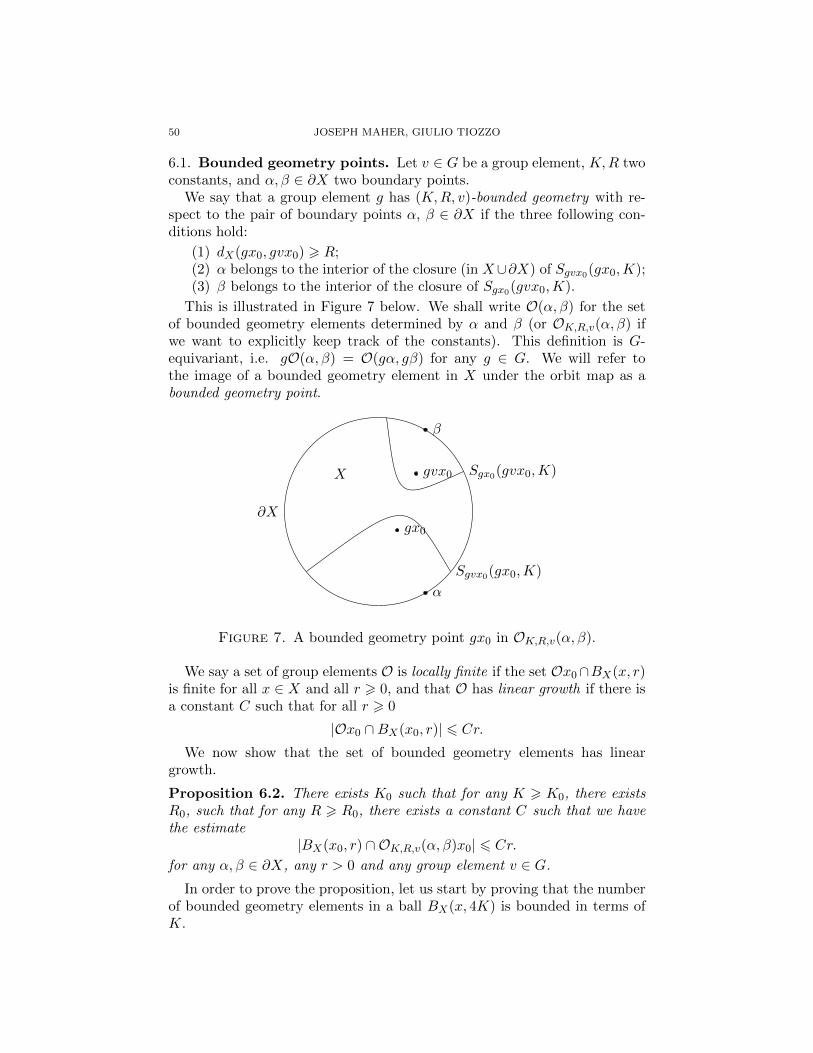
50 JOSEPH MAHER, GIULIO TIOZZO
6.1. Bounded geometry points. Let v ∈ G be a group element, K,R twoconstants, and α, β ∈ ∂X two boundary points.
We say that a group element g has (K,R, v)-bounded geometry with re-spect to the pair of boundary points α, β ∈ ∂X if the three following con-ditions hold:
(1) dX(gx0, gvx0) > R;(2) α belongs to the interior of the closure (in X∪∂X) of Sgvx0(gx0,K);(3) β belongs to the interior of the closure of Sgx0(gvx0,K).
This is illustrated in Figure 7 below. We shall write O(α, β) for the setof bounded geometry elements determined by α and β (or OK,R,v(α, β) ifwe want to explicitly keep track of the constants). This definition is G-equivariant, i.e. gO(α, β) = O(gα, gβ) for any g ∈ G. We will refer tothe image of a bounded geometry element in X under the orbit map as abounded geometry point.
β
α
Sgx0(gvx0,K)
Sgvx0(gx0,K)
gx0
gvx0X
∂X
Figure 7. A bounded geometry point gx0 in OK,R,v(α, β).
We say a set of group elements O is locally finite if the set Ox0∩BX(x, r)is finite for all x ∈ X and all r > 0, and that O has linear growth if there isa constant C such that for all r > 0
|Ox0 ∩BX(x0, r)| 6 Cr.We now show that the set of bounded geometry elements has linear
growth.
Proposition 6.2. There exists K0 such that for any K > K0, there existsR0, such that for any R > R0, there exists a constant C such that we havethe estimate
|BX(x0, r) ∩ OK,R,v(α, β)x0| 6 Cr.for any α, β ∈ ∂X, any r > 0 and any group element v ∈ G.
In order to prove the proposition, let us start by proving that the numberof bounded geometry elements in a ball BX(x, 4K) is bounded in terms ofK.

RANDOM WALKS ON WEAKLY HYPERBOLIC GROUPS 51
Lemma 6.3. There exists K0 such that, for any K > K0, there exists R0
such that for any R > R0 and any group element v ∈ G, we have the estimate
|BX(x, 4K) ∩ OK,R,v(α, β)x0| 6 N(22K)
for any pair of boundary points α and β, and any point x ∈ X.
γ
fγ
x
BX(x, 4K)
gx0
p
6 2K
fgx0
6 2K
gvx0
q
6 2K
fgvx0
r
6 2K
Figure 8. Bounded geometry points in BX(x, 4K).
Proof. Recall from Section 2.3 that we have chosen Q and c to be two num-bers such that every pair of points in the Gromov boundary ∂X are con-nected by a continuous (Q, c)-quasigeodesic. We shall choose L to be a Morseconstant for the (Q, c)-quasigeodesics, i.e. for any pair of points x and y ina (Q, c)-quasigeodesic γ, the segment of γ between x and y is contained inan L-neighbourhood of any geodesic connecting x and y.
Let g be a bounded geometry element, and write S1 for Sgvx0(gx0,K) andS2 for Sgx0(gvx0,K). As g has bounded geometry, each (Q, c)-quasigeodesicfrom α to β passes within distance L+K+O(δ) of both gx0 and gvx0. There-fore we may choose K0 to be sufficiently large such that for any K > K0
the distance from any bounded geometry point gx0 to a (Q, c)-quasigeodesicconnecting α and β is at most 2K. Furthermore, we will choose K0 to belarger than the quasigeodesic constants Q and c, and also larger than theMorse constant L.
Given K, we will choose R0 sufficiently large such that for any (Q, c)-quasigeodesic γ with one endpoint in the interior of S1, and the other end-point in the interior of S2, the nearest point projections of S1 and S2 ontoγ are disjoint. Furthermore, we shall choose R0 to be at least the acylindri-cality constant R(22K).
Let gx0 and g′x0 ∈ BX(x, 4K)∩OK,R,v(α, β)x0 be two bounded geometryelements with respect to the same boundary points (α, β), and the sameelement v. We may write g′ = fg, for some group element f ∈ G. This isillustrated in Figure 8 above. The isometry f moves the point gx0 distanceat most 8K.
Now let γ be a (Q, c)-quasigeodesic joining α to β. By construction,both γ and fγ have endpoints in fS1 and fS2, hence they both pass within

52 JOSEPH MAHER, GIULIO TIOZZO
distance 2K from both fgx0 and fgvx0. Let us now consider y := gvx0; wenow show that the isometry f also moves the point y a bounded distance,which yields the claim by definition of an acylindrical action.
Let p be a closest point on γ to gx0, let q be a closest point on γ to gvx0,and let r be a closest point on γ to fgvx0. As the shadows S1 and S2 havedisjoint nearest point projections to γ, the order in which the three pointsappear on γ is either (p, q, r) or (p, r, q). As the distances from p to r and pto q are both approximately dX(x0, vx0), this implies that dX(q, r) is small;we now make this precise.
Claim 6.4. dX(q, r) 6 18K.
Proof (of claim). The point p is within distance 2K of gx0, and the point qis within distance 2K of gvx0, so
|dX(p, q)− dX(gx0, gvx0)| 6 4K.
Similarly, the point p is within distance 10K of fgx0, and the point r iswithin distance 2K of fgvx0, so
|dX(p, r)− dX(fgx0, fgvx0)| 6 12K.
Combining these two estimates and using dX(gx0, gvx0) = dX(fgx0, fgvx0)gives
(30) |dX(p, q)− dX(p, r)| 6 16K.
First consider the case in which the order is (p, q, r). As γ is a (Q, c)-quasigeodesic, the point q lies within distance L of a geodesic from p to r:if we denote q′ the projection of q onto this geodesic segment, then we have
dX(q′, r) = dX(p, r)− dX(p, q′)
which, using the fact that q′ is within distance L from q, gives
dX(q, r) 6 dX(p, r)− dX(p, q) + 2L
and now combining this with the estimate (30) one gets
dX(q, r) 6 16K + 2L 6 18K.
If the points lie on γ in the order (p, r, q), the proof is analogous.
As q is close to gvx0 and r is close to fgvx0, we obtain the followingestimate
dX(gvx0, fgvx0) 6 22K.
Therefore, f moves each of gx0 and gvx0 distance at most 22K, and so byacylindricality there are at most N(22K) possible choices for f , as we havechosen R0 > R(22K), as required.
Proof of Proposition 6.2. Let γ be a (Q, c)-quasigeodesic connecting α andβ. We shall choose the number K0 to be the same as the number K0 fromLemma 6.3. Then K is sufficiently large such that every element of O(α, β)has an image in X which lies within distance at most 2K of γ, and any pair

RANDOM WALKS ON WEAKLY HYPERBOLIC GROUPS 53
of points γ(n) and γ(n + 1) on the quasigeodesic are distance at most 2Kapart. Therefore O(α, β)x0 is covered by balls of the form BX(γ(n), 4K)for n ∈ N, and the claim follows from applying Lemma 6.3 to each of theseballs.
6.2. Recurrence and the strip criterion. Given a bi-infinite sample path(wn)n∈Z, we shall define the forward and backward limit points to be
λ+(ω) := limn→∞
wnx0, and λ−(ω) := limn→∞
w−nx0.
As the forward and backward random walks converge to the Gromov bound-ary, these limit points are defined for P-almost all ω, and the joint distribu-tion of the pair (λ+(ω), λ−(ω)) is ν × ν.
For any bi-infinite sequence ω ∈ Ω = GZ, we define O(ω) to be the setO(λ+(ω), λ−(ω)) of bounded geometry elements determined by the limitpoint λ+(ω) of the forward random walk and the limit point λ−(ω) of thebackward random walk.
Finally, we show that we can choose K, R, and v such that the set ofbounded geometry elements is non-empty and locally finite for ν× ν-almostall (α, β) ∈ ∂X × ∂X.
Proposition 6.5. There are constants K,R and a group element v ∈ Gsuch that the set
OK,R,v(α, β)
of bounded geometry elements has linear growth and is non-empty (in fact,infinite) for ν × ν-almost all pairs (α, β).
Proof. By Proposition 5.4, we can choose K large enough so that for anygroup element v, the closure of the shadow S = Sx0(vx0,K) has positiveν-measure, and the closure of the shadow S′ = Svx0(x0,K) has positiveν-measure. Thus, the probability that the group identity element 1 lies inO(ω) is positive, because
P (ω : 1 ∈ O(ω)) = ν(S)ν(S′) = p > 0.
Consider the probability that the location of the random walk wn lies inO(ω), i.e.
P (ω : wn ∈ O(λ+(ω), λ−(ω))) .
By G-equivariance, this is equal to
P(ω : 1 ∈ O(w−1
n λ+(ω), w−1n λ−(ω))
),
and by definition of the shift map this is equal to
P (ω : 1 ∈ O(Tnω)) .
As the shift map preserves the measure P, this is equal to
P (ω : 1 ∈ O(ω)) = p > 0.

54 JOSEPH MAHER, GIULIO TIOZZO
Therefore the events ω ∈ Ω : wn ∈ O(ω) occur with the same positiveprobability p, though they are not independent. By ergodicity of the shiftmap, the proportion of locations w1, . . . wN satisfying wn ∈ O(ω) con-verges to p as N tends to infinity. As (wnx0)n∈N converges to the boundaryP-almost surely, O(ω) contains infinitely many elements P-almost surely.
We remind the reader of Kaimanovich’s strip criterion from [Kai00, The-orem 6.4]. We shall write BG(1, r) for all group elements whose image in Xunder the orbit map is distance at most r from the basepoint x0, i.e.
BG(1, r) = g ∈ G | dX(x0, gx0) 6 r.
Theorem 6.6. Let µ be a probability measure with finite entropy on G, andlet (∂X, ν) and (∂X, ν) be µ- and µ-boundaries, respectively. If there existsa measurable G-equivariant map S assigning to almost every pair of points(α, β) ∈ ∂X × ∂X a non-empty “strip” S(α, β) ⊂ G, such that for all g
1
nlog |S(α, β)g ∩BG(1, dX(x0, wnx0))| → 0 as n→∞,
for (ν × ν)-almost every (α, β) ∈ ∂X × ∂X, then (∂X, ν) and (∂X, ν) arethe Poisson boundaries of the random walks (G,µ) and (G, µ), respectively.
In order to prove Theorem 1.5, we define the strip S(α, β) as the setOK,R,v(α, β) of bounded geometry elements. By right multiplication byg−1, the set
S(α, β)g ∩BG(1, dX(x0, wnx0))
has the same cardinality as
S(α, β) ∩BG(1, dX(x0, wnx0))g−1.
Furthermore,
BG(1, dX(x0, wnx0))g−1 ⊂ BG(1, dX(x0, wnx0) + dX(x0, gx0)),
and so
|S(α, β)g ∩BG(1, dX(x0, wnx0))| 6 |S(α, β) ∩BG(1, dX(x0, wnx0) + dX(x0, gx0))| .
Proposition 6.5 shows that there are suitable choices of K,R and v suchthat the sets of bounded geometry elements are non-empty almost surelyand have linear growth, so there is a number K such that
|S(α, β)g ∩BG(1, dX(x0, wnx0))| 6 K(dX(x0, wnx0) + dX(x0, gx0)).
Therefore, it suffices to show that almost surely log dX(x0, wnx0)/n → 0as n → ∞, and this follows from the fact that µ has finite logarithmicmoment, as we now briefly explain. Finite logarithmic moment implies thatlog dX(x0, gnx0)/n → 0 almost surely, and so for any ε > 0 there exists aC > 1 such that we have dX(x0, gnx0) 6 Ceεn for all n. By the triangleinequality
dX(x0, wnx0) 6 dX(x0, g1x0) + · · ·+ dX(x0, gnx0),

RANDOM WALKS ON WEAKLY HYPERBOLIC GROUPS 55
and so
log dX(x0, wnx0) 6 logC + log n+ εn.
As this holds for all ε > 0, this implies that log dX(x0, wnx0)/n → 0 asn→∞, as required.
Finally, the statement that the map S is measurable means that for anyg ∈ G, the set
(α, β) ∈ ∂X × ∂X | g ∈ S(α, β)
is a Borel set; this holds, since by definition, g ∈ S(α, β) if and only if (α, β)belongs to the product of the closures of two shadows, which is closed, henceBorel. This completes the proof of Theorem 1.5.
Appendix A. Estimating translation length
In this section we provide a proof of Proposition 5.8, which estimates thetranslation length in terms of the distance an isometry moves the basepoint,and the Gromov product.
Proposition 5.8. There exists a constant C0 > 0, which depends only onδ, such that the following holds. For any isometry g of a δ-hyperbolic spaceX, if g satisfies the inequality
(31) dX(x0, gx0) > 2(gx0 · g−1x0)x0 + C0,
then the translation length of g is
(32) τ(g) = dX(x0, gx0)− 2(g−1x0 · gx0)x0 +O(δ).
Proof. We start by showing that if γ is a geodesic segment from x0 to gnx0,then gkx0 is contained in a bounded neighbourhood of γ, for all 0 6 k 6 n.We shall write xk for gkx0. Note that, since the action is isometric, we havefor each k
(33) dX(xk+1, xk+2) = dX(x0, gx0), and (xk · xk+2)xk+1= (gx0 · g−1x0)x0 .
Claim A.1. Let γ be a geodesic from x0 to xn. Then
(34) dX(xk, γ) 6 (gx0 · g−1x0)x0 +O(δ),
for all 0 6 k 6 n.
Proof (of claim). Let pk be a nearest point on γ to xk, and let xk be anelement of xknk=0 furthest from γ. Consider the quadrilateral formed byxk−1, xk+1, pk+1 and pk−1, as illustrated below in Figure 9.

56 JOSEPH MAHER, GIULIO TIOZZO
x0 γ xnpk−1 pk+1
xk−1q
xk+1
xk
Figure 9. The points xk = gkx0 lie in a bounded neigh-bourhood of γ.
Let q be a nearest point to xk on a geodesic segment from xk−1 to xk+1.By the estimate for the Gromov product in terms of distance to a geodesic(1),
(xk−1 · xk+1)xk = dX(xk, [xk−1, xk+1]) +O(δ),
and as g is an isometry, this implies that
dX(xk, q) = (gx0 · g−1x0)x0 +O(δ).
By thin triangles, the point q lies within distance 2δ of at least one of theother three sides of the quadrilateral. Suppose q lies within 2δ of a geodesicfrom xk−1 to pk−1.
Since xk is the furthest point from the geodesic γ, we have dX(xk, γ) >dX(xk−1, γ), and since q lies in a 2δ-neighbourhood of the geodesic fromxk−1 to pk−1, we have
(35) dX(xk−1, q) 6 dX(xk, q) +O(δ).
On the other hand, if we now assume (31) and apply the reverse triangleinequality (3), we get
dX(xk, xk−1) = dX(xk, q) + dX(xk−1, q) +O(δ)
dX(xk, xk−1) > 2dX(xk, q) + C0 +O(δ)
hence
dX(xk−1, q) > dX(xk, q) + C0 +O(δ),
which contradicts (35) if C0 is large enough (depending only on δ). Thesame argument applies if q lies within 2δ of a geodesic from xk+1 to pk+1.Therefore, q lies within 2δ of γ, and so dX(xk, γ) 6 (gx0 · g−1x0)x0 + O(δ),as required.
Consider a pair of adjacent points xk and xk+1. Combining (31), (34),and the triangle inequality, gives
(36) dX(pk, pk+1) > dX(x0, gx0)− 2(gx0 · g−1x0)x0 +O(δ).

RANDOM WALKS ON WEAKLY HYPERBOLIC GROUPS 57
Consider a triple of consecutive points, xk, xk+1 and xk+2. If their corre-sponding nearest point projections pk, pk+1 and pk+2 to γ do not lie in thesame order, then using Proposition 2.3 repeatedly one gets, if pk+2 lies inbetween pk and pk+1, the equality
(xk · xk+2)xk+1= dX(xk+1, xk+2)− dX(xk+2, pk+2) +O(δ)
which, using (33) and (34), implies
dX(x0, gx0)− 2(gx0 · g−1x0)x0 = O(δ)
which contradicts (31) if C0 is large enough. The case where pk lies betweenpk+1 and pk+2 is completely analogous, therefore the pk are monotonicallyordered on γ, and so by (36)
dX(p0, pk) > k(dX(x0, gx0)− 2(gx0 · g−1x0)x0 +O(δ)),
which implies, by Proposition 2.3, a similar bound for dX(x0, xk), and so infact (xk)k∈N is quasi-geodesic, with τ(g) > dX(x0, gx0)− 2(gx0 · g−1x0)x0 +O(δ).
The upper bound on τ(g) follows from the triangle inequality; indeed, foreach y ∈ X one has
τ(g) 6 dX(y, gy)
and the desired bound follows by taking as y the midpoint of the geodesicsegment between x0 and gx0, completing the proof of Proposition 5.8.
References
[AB06] Charalambos D. Aliprantis and Kim C. Border, Infinite dimensional analysis,3rd ed., Springer, Berlin, 2006.
[BDL14] Uri Bader, Bruno Duchesne, and Jean Lecureux, Furstenberg maps for CAT(0)targets of finite telescopic dimension (2014), available at arXiv:1404.3187.
[BGS85] Werner Ballmann, Mikhael Gromov, and Viktor Schroeder, Manifolds of non-positive curvature, Progress in Mathematics, vol. 61, Birkhauser Boston, Inc.,Boston, MA, 1985.
[BBF10] Mladen Bestvina, Kenneth Bromberg, and Koji Fujiwara, Constructing groupactions on quasi-trees and applications to mapping class groups (2010), availableat arXiv:1006.1939.
[BF10] Mladen Bestvina and Mark Feighn, A hyperbolic Out(Fn)-complex, GroupsGeom. Dyn. 4 (2010), no. 1, 31–58.
[BF14] Mladen Bestvina and Mark Feighn, Hyperbolicity of the complex of free factors,Adv. Math. 256 (2014), 104–155.
[Bjo10] Michael Bjorklund, Central limit theorems for Gromov hyperbolic groups, J.Theoret. Probab. 23 (2010), no. 3, 871–887.
[BHM11] Sebastien Blachere, Peter Haıssinsky, and Pierre Mathieu, Harmonic measures
versus quasiconformal measures for hyperbolic groups, Ann. Sci. Ec. Norm.Super. (4) 44 (2011), no. 4, 683–721.
[BS00] M. Bonk and O. Schramm, Embeddings of Gromov hyperbolic spaces, Geom.Funct. Anal. 10 (2000), no. 2, 266–306.
[Bow08] Brian H. Bowditch, Tight geodesics in the curve complex, Invent. Math. 171(2008), no. 2, 281–300.
[Bri12] Martin R. Bridson, On the dimension of CAT(0) spaces where mapping classgroups act, J. Reine Angew. Math. 673 (2012), 55–68.
58 JOSEPH MAHER, GIULIO TIOZZO
[BH99] Martin R. Bridson and Andre Haefliger, Metric spaces of non-positive curvature,Grundlehren der Mathematischen Wissenschaften [Fundamental Principles ofMathematical Sciences], vol. 319, Springer-Verlag, Berlin, 1999.
[CM15] Danny Calegari and Joseph Maher, Statistics and compression of scl, ErgodicTheory Dynam. Systems 35 (2015), no. 1, 64–110.
[DP12] Thomas Delzant and Pierre Py, Kahler groups, real hyperbolic spaces and theCremona group, Compos. Math. 148 (2012), no. 1, 153–184.
[Duc05] Moon Duchin, Geodesics track random walks in Teichmuller space, ProQuestLLC, Ann Arbor, MI, 2005. Thesis (Ph.D.)–The University of Chicago.
[Fuj08] Koji Fujiwara, Subgroups generated by two pseudo-Anosov elements in a map-ping class group. I. Uniform exponential growth, Groups of diffeomorphisms,Adv. Stud. Pure Math., vol. 52, Math. Soc. Japan, Tokyo, 2008, pp. 283–296.
[Fur63] Harry Furstenberg, Noncommuting random products, Trans. Amer. Math. Soc.108 (1963), 377–428.
[GM12] Francois Gautero and Frederic Matheus, Poisson boundary of groups acting onR-trees, Israel J. Math. 191 (2012), no. 2, 585–646.
[Gui80] Y. Guivarc’h, Sur la loi des grands nombres et le rayon spectral d’une marchealeatoire, Conference on Random Walks (Kleebach, 1979), Asterisque, vol. 74,Soc. Math. France, Paris, 1980, pp. 47–98, 3 (French, with English summary).
[Har86] John L. Harer, The virtual cohomological dimension of the mapping class groupof an orientable surface, Invent. Math. 84 (1986), no. 1, 157–176.
[Ham06] Ursula Hamenstadt, Train tracks and the Gromov boundary of the complexof curves, Spaces of Kleinian groups, London Math. Soc. Lecture Note Ser.,vol. 329, Cambridge Univ. Press, Cambridge, 2006, pp. 187–207.
[HM13] Michael Handel and Lee Mosher, The free splitting complex of a free group, I:hyperbolicity, Geom. Topol. 17 (2013), no. 3, 1581–1672.
[Hor14] Camille Horbez, The Poisson boundary of Out(FN ) (2014), available at arXiv:1405.7938.
[Kai87] V. A. Kaimanovich, Lyapunov exponents, symmetric spaces and a multiplica-tive ergodic theorem for semisimple Lie groups, Zap. Nauchn. Sem. Leningrad.Otdel. Mat. Inst. Steklov. (LOMI) 164 (1987), no. Differentsialnaya Geom.Gruppy Li i Mekh. IX, 29–46, 196–197 (Russian, with English summary); Eng-lish transl., J. Soviet Math. 47 (1989), no. 2, 2387–2398.
[Kai94] Vadim A. Kaimanovich, The Poisson boundary of hyperbolic groups, C. R. Acad.Sci. Paris Ser. I Math. 318 (1994), no. 1, 59–64 (English, with English andFrench summaries).
[Kai00] Vadim A. Kaimanovich, The Poisson formula for groups with hyperbolic prop-erties, Ann. of Math. (2) 152 (2000), no. 3, 659–692.
[KM96] Vadim A. Kaimanovich and Howard A. Masur, The Poisson boundary of themapping class group, Invent. Math. 125 (1996), no. 2, 221–264.
[KB02] Ilya Kapovich and Nadia Benakli, Boundaries of hyperbolic groups, Combina-torial and geometric group theory (New York, 2000/Hoboken, NJ, 2001), Con-temp. Math., vol. 296, Amer. Math. Soc., Providence, RI, 2002, pp. 39–93.
[KL96] Michael Kapovich and Bernhard Leeb, Actions of discrete groups on nonposi-tively curved spaces, Math. Ann. 306 (1996), no. 2, 341–352.
[KL06] Anders Karlsson and Francois Ledrappier, On laws of large numbers for randomwalks, Ann. Probab. 34 (2006), no. 5, 1693–1706.
[KL07] Anders Karlsson and Francois Ledrappier, Linear drift and Poisson boundaryfor random walks, Pure Appl. Math. Q. 3 (2007), no. 4, Special Issue: In honorof Grigory Margulis., 1027–1036.
[KK13] Sang-hyun Kim and Thomas Koberda, Embedability between right-angled Artingroups, Geom. Topol. 17 (2013), no. 1, 493–530.
RANDOM WALKS ON WEAKLY HYPERBOLIC GROUPS 59
[KK14] Sang-Hyun Kim and Thomas Koberda, The geometry of the curve graph of aright-angled Artin group, Internat. J. Algebra Comput. 24 (2014), no. 2, 121–169.
[Kin68] J. F. C. Kingman, The ergodic theory of subadditive stochastic processes, J. Roy.Statist. Soc. Ser. B 30 (1968), 499–510.
[Kla] E. Klarreich, The boundary at infinity of the curve complex and the relativeTeichmuller space.
[Kow08] E. Kowalski, The large sieve and its applications, Cambridge Tracts in Math-ematics, vol. 175, Cambridge University Press, Cambridge, 2008. Arithmeticgeometry, random walks and discrete groups.
[Led01] Francois Ledrappier, Some asymptotic properties of random walks on freegroups, Topics in probability and Lie groups: boundary theory, CRM Proc.Lecture Notes, vol. 28, Amer. Math. Soc., Providence, RI, 2001, pp. 117–152.
[Mah10a] Joseph Maher, Linear progress in the complex of curves, Trans. Amer. Math.Soc. 362 (2010), no. 6, 2963–2991.
[Mah10b] Joseph Maher, Random Heegaard splittings, J. Topol. 3 (2010), no. 4, 997–1025.[Mah11] Joseph Maher, Random walks on the mapping class group, Duke Math. J. 156
(2011), no. 3, 429–468.[Mah12] Joseph Maher, Exponential decay in the mapping class group, J. Lond. Math.
Soc. (2) 86 (2012), no. 2, 366–386.[MS14] A. Malyutin and P. Svetlov, Poisson–Furstenberg boundaries of fundamental
groups of closed 3-manifolds (2014), available at arXiv:1403.2135.[Man74] Yu. I. Manin, Cubic forms: algebra, geometry, arithmetic, North-Holland Pub-
lishing Co., Amsterdam-London; American Elsevier Publishing Co., New York,1974. Translated from the Russian by M. Hazewinkel; North-Holland Mathe-matical Library, Vol. 4.
[Mar91] G. A. Margulis, Discrete subgroups of semisimple Lie groups, Ergebnisse derMathematik und ihrer Grenzgebiete (3) [Results in Mathematics and RelatedAreas (3)], vol. 17, Springer-Verlag, Berlin, 1991.
[MM99] Howard A. Masur and Yair N. Minsky, Geometry of the complex of curves. I.Hyperbolicity, Invent. Math. 138 (1999), no. 1, 103–149.
[MS14] Pierre Mathieu and Alessandro Sisto, Deviation inequalities for random walks(2014), available at arXiv:1411.7865.
[NS13] Amos Nevo and Michah Sageev, The Poisson boundary of CAT(0) cube complexgroups, Groups Geom. Dyn. 7 (2013), no. 3, 653–695.
[Ose68] V. I. Oseledec, A multiplicative ergodic theorem. Characteristic Ljapunov, ex-ponents of dynamical systems, Trudy Moskov. Mat. Obsc. 19 (1968), 179–210(Russian).
[Osi13] Dennis Osin, Acylindrically hyperbolic groups (2013), available at arXiv:1304.
1246.[Riv08] Igor Rivin, Walks on groups, counting reducible matrices, polynomials, and sur-
face and free group automorphisms, Duke Math. J. 142 (2008), no. 2, 353–379.[Sel97] Z. Sela, Acylindrical accessibility for groups, Invent. Math. 129 (1997), no. 3,
527–565.[Sis11] Alessandro Sisto, Contracting elements and random walks (2011), available at
arXiv:1112.2666.[Sis13] Alessandro Sisto, Tracking rates for random walks (2013), available at arXiv:
1305.5472.[Tio12] Giulio Tiozzo, Sublinear deviation between geodesics and sample paths (2012).
to appear on Duke Math. J.[Vai05] Jussi Vaisala, Gromov hyperbolic spaces, Expo. Math. 23 (2005), no. 3, 187–231.
[Woe00] Wolfgang Woess, Random walks on infinite graphs and groups, CambridgeTracts in Mathematics, vol. 138, Cambridge University Press, Cambridge, 2000.

60 JOSEPH MAHER, GIULIO TIOZZO
Joseph MaherCUNY College of Staten Island and CUNY Graduate [email protected]
Giulio TiozzoYale [email protected]