The choice between public and private schools with or without subsidies in SpainManuel Arellano Gema ZamarroCEMFI, Madrid Tilburg University

IntroductionWhat choice for Spanish parents?

• The majority of parents with children of compulsory schooling age face a choice be-tween a state school and a concerted private school, neither of which will, in principle,charge fees because they are both funded through the taxpayer, and are supposed to pro-vide their services free. In practice, parents do meet some out-of-pocket expenses, butmuch smaller than those faced by the small fraction of parents that send their childrento non-concerted fee-paying private schools.

• A concerted school is a private school, typically Catholic (80%), that signs a long-termconcert with the government by which it becomes fully subsidized in exchange for im-plementing a state school-like admission policy. The concert stipulates that teachers’salaries are paid directly by the government, and that the school should have an exter-nal governing body with the power of hiring and firing the school head.

• Large scale subsidies to the private sector began in the post-Franco period, and con-certed schools were introduced in 1984. The aims were to ensure the provision of freeplaces and to preserve a role for Catholic schools, following the reform that orderedfree and compulsory schooling from age 6 to 14.

Concerts, voucher programs, and charter schools

• Public subsidies to private schools exist under different schemes in several countries.• A feature of Spanish concerted schooling is the large size of the scheme, with an en-rollment rate of about 25% and public funding of 3,7 billion euro in 2003.

• Another feature is that the system was not designed to create competition betweenschools, as is the case with voucher programs whereby a private school receives avoucher for each enrolled student.

• Voucher programs often allow households to choose private schools without residencerestrictions. However, admission to Spanish concerted schools is subject to the sameresidence requirements as state schools.

• Concerted schools bear resemblancewith but are different from charter schools as existin the US and other countries. A charter school is an autonomous public school thatis freed from some of the rules of ordinary public schools in exchange for some formof accountability for schooling outcomes. Instead, a concerted school is a privatelyowned school that is tied by the rules of ordinary public schools in exchange for publicfunding.

2

Concerted schools and immigration

• Recently, public policy towards concerted schools has been the subject of controversyin the wake of previously unseen immigration flows from non-EU countries; e.g. thenumber of immigrant children in Madrid increased by 350% between 1999 and 2003.

• Applications for concerted schools, specially in large urban areas, have soared. In 1999the number of concerted schools increased substantially in the Madrid region, after thetransfer of public education from the central to the regional government, which favoredparents’ ‘‘freedom of choice’’ and that the allocation of funds should be determined bysupply and demand. A similar path has been followed in other regions.

• Critics argued that in practice concerted schools are not service-free because they offeran additional, nominally optional, hour of teaching, which is charged as voluntary aid,among other extracurricular activities.

• Their argument is that students with special needs (basically immigrants) concentratein public schools, which are disproportionately located in low-income and rural areas,and that an excessive concentration may have an adverse effect on the others.

• Conversely, by locating in affluent areas and charging higher (yet highly subsidized)fees, concerted schools could self-select children from parents with highly educatedbackgrounds and hence enjoymore peer-effect capital and less social conflict than stateschools, so that concerted schooling operates as a subsidy for middle class parents.

3

This paper

• A natural ingredient of an empirical assessment of concerted schooling is to see howmuch individual probabilities of attending a given school type differ by parental educa-tion and income, after controlling by household composition, location, and preferencesfor religious education. Unfortunately, school choice is conspicuously absent from themajor Spanish socioeconomic household surveys.

• An exception is the last large cross-sectional family expenditure survey (EPF), con-ducted in 1990. This survey provided detailed information on household composition,income, and expenditures, including schooling expenditures, and whether children, ifpresent, went to a public or private school. However, the survey made no distinctionbetween concerted and non-concerted private schools.

• In this paper we provide evidence on the determinants of the choice between public,concerted, and fee-paying private schools using data drawn from the EPF survey.

• Our strategy to identify separately probabilities for concerted and non-concerted schoolchoices is to rely on schooling expenditure variables, which induce a natural separationin the data. We achieve this by specifying a joint mixture likelihood model of schoolchoice and education expenditures.

• Moreover, we construct a measure of preferences for religious schooling from a binarymodel of church attendance estimated on a complementary dataset.

4

Outline

1. Theoretical framework.

2. The Spanish schooling system.

3. Data.

4. Econometric methodology.

5. Empirical results.

5

Theoretical framework

• The Spanish schooling system is characterized by two different levels of choice: choiceamong school enrollment areas (‘‘area de influencia’’) and choice between public, con-certed, and private schools.

Choice of residential location

• The former takes place by choosing a residential location. Spanish authorities operate ascheme of catchment areas for all primary and secondary public and concerted schools.There is no guarantee of a place for pupils resident within a catchment area, but livingin a catchment area gives pupils a higher priority for admission.

• Assuming that households choose a location based on the quality of the schools andhouse prices, Nesheim (2005) shows that in an economy populated by householdswith heterogeneous incomes and abilities in which the quality of schools in a locationis only determined by the residents of the location, a sorting equilibrium results.

• In this setting, an influx of immigrants may change the distribution of incomes andabilities, hence altering the sorting equilibrium.

6

Choice of school type given location

• The second level of choice is between public, concerted, and private schools within aresidential location. There is evidence that concerted schools are not evenly distributedacross areas but that tend to be over-represented in relatively high income locations.

• Within a location, the school choice of households can be analyzed in a model ofcompetition between private and public schools with peer-group externalities as inEpple and Romano (1998).

• Suppose household’s utility is increasing in consumption and the child’s educationalachievement. Let y be income, pj (j = 1, 2, 3) tuition expenditure by school type, anda = a (θj, b) achievement (e.g. test scores) as a function of child’s ability b and themean ability of the students at the school attended θj. The utility of alternative j is

Uj = U (y − pj, a (θj, b)) .• A household is characterized by an ability–income pair (b, y). The achievement func-tion captures the peer effect. Households choose a private or public school taking p andθ as given, but in equilibrium an Epple-Romano type of model will predict a hierarchyof school qualities with public schools having the lowest ability peer group.

• Households’ valuation of the quality of the school may depend on its preferences forCatholic schooling, in which case the utility of alternative j should be augmented bya preference parameter rj.

7

Cobb-Douglas model

• Assuming a Cobb-Douglas specification of the utility functionUj = (y − pj) θγj bβerj (j = 1, 2, 3) ,

a logistic assumption leads to the following odd ratios

lnPr (2)

Pr (1)= ln

µy − p2y

¶+ γ ln

µθ2θ1

¶+ r2 ' γ ln

µθ2θ1

¶− p21

y+ r2

lnPr (3)

Pr (1)= ln

µy − p3y

¶+ γ ln

µθ3θ1

¶+ r3 ' γ ln

µθ3θ1

¶− p31

y+ r3.

• The parameter γ, which captures household preferences for school quality, may berelated to observable characteristics such as parental schooling.

• Relative school qualities θj/θ1 will vary with income and ability across locations, andtherefore will be associated with location variables such as house prices.

• There will be endogenous variation in the supply of different types of school by loca-tion.

• Community models with peer group effects predict that the distribution of householdcharacteristics is one of the main determinants of the shape of the sorting equilibrium.

• Therefore, across large geographical areas, such as provinces or regions, we wouldexpect individual reduced-form school choice probabilities to vary with regional-leveldistributional characteristics, like income, after conditioning on individual attributes.

8

The Spanish school system

• Three major bills (1970, 1985, and 1990) built the modern Spanish school system. The1970 act mandated free and compulsory schooling for children 6 to 14, but at the timethere were not enough places to enforce the law. A program of school construction wasinsufficient to cover the demand created by regional migration and the ‘‘baby boom’’.

• At the return to democracy in 1977, a high proportion of pupils (40%) were in fee-paying private schools, and there was an unsatisfied demand for state school slots.

• The government’s answer was to subsidize private schools to enable them provide theirservices free. Most private schools accepted the deal.

• At first, government funded private schools retained the freedom to choose admissionpolicies. This situation changedwith the 1984 reform, whichmade funding conditionalon state-school admission policy and free education. However, some kept charging fornominally voluntary contributions, usually on account of extracurricular activities.

• A relatively small number of private schools chose to remain non-concerted. These arefee-paying schools that in this way retained the ability to choose selective admissionand tuition policies. This category includes academically or socially selective schools,some religious denominations, and foreign-language oriented schools.

• Finally, the 1990 reform extended compulsory education to the age of sixteen, andundertook to provide free but optional pre-school education to children aged 4 to 6.

9

Evidence on public and private school outcomes from test scores

• There are two recent sources of information about average scores from standardizedcognitive tests administered to 6th grade children (aged 11–12).

• The first one was conducted at schools in the region of Madrid in 2005.• As shown in Table 1, average maths scores at concerted and private schools are 8 and11 percent higher, respectively, than the public school maths score. The difference forthe reading scores is almost twice as large, probably reflecting a higher fraction offoreign-born pupils at public schools.

Table 1Average test scores at age 11–12f

Public Concerted Privatetest score score % public score % public

Reading 55 63 15% 67 22%Maths 56 60.5 8% 62 11%

No. of schools 701 (60%) 356 (31%) 103 (9%)fPupils from all schools in the region of Madrid tested in 2005.

Source: Trillo del Pozo et al. (2006), tables 3 and 4.

10

Test scores (continued)

• The other piece of information is a test administered to a sample of pupils from 450Spanish schools as part of a government evaluation exercise (see INECSE, 2003).

• Unfortunately, this source does not distinguish between concerted and non-concertedprivate schools.

• Scores for general knowledge, reading, and maths tests at public schools were 64, 64,and 56, respectively, to be compared with 69, 68, and 61 at private schools.

• The differences are broadly comparable with those from the previous source, speciallyfor the maths scores.

• These figures provide relevant background for our empirical analysis, but they are onlyindirectly relevant to the results we present, which belong to an earlier period.

11

The data

• The cross-sectional micro data used in this paper comes from the 1990 Spanish house-hold expenditure survey (EPF). We selected a sample of households with:(a) children aged less than 16, in elementary school.(b) the same type of school for all children when more than one is present.

• The EPF contains detailed information about family expenditures, including expendi-tures on registration and tuition fees, and other schooling-related expenditures.

• A limitation: the EPF provides information on whether children are in a public or pri-vate school, but without distinguishing between concerted and non-concerted schools.

• The final sample consists of 5427 households, of which 77% chose a public school.• Public school families have less educated parents, earn lower salaries, have a higherproportion of non-working mothers, are less likely to have a second home, and live insmaller districts (Table 2B).

• Table 3 shows expenditures in education by type of school. In principle, registrationand tuition fees should be zero for both public and concerted schools, but in practicesome concerted schools are perceived by parents as charging for such concepts.

• Table 4 shows registration and tuition expenditure quantiles. We use this variation toidentify separate determinants of choice of concerted and non-concerted schools.

12

Table 4Quantile distribution of registration and tuition fees in private schoolsf

Percentile Centile registration fees Centile tuition fees5 0 040 0 050 0 15.0260 0 72.1270 0 129.9475 0 158.0780 9.02 198.3385 18.03 256.7590 28.67 420.7195 42.07 715.8199 102.17 1622.73

f In euros.

13

An econometric model for school choice with incomplete data

• We show how to estimate a multinomial model of the choice between the three types ofschools (public, concerted and private) when we only observe if the household choosesa public school or not, but we have information on expenditure in education.

• LetD1i,D2i, andD3i be indicators of public, concerted private, and fee-paying privateschool, respectively.

• OnlyD1i is observable, but we also observe expenditure on educational items.• The idea of our method is to consider the joint likelihood of schooling expenditure andobserved binary school type as a function of the underlying multinomial probabilities.

• Letting wi denote the schooling expenditure of household i, the joint likelihood ofexpenditure and observed school type is:

L =YD1i=1

f (wi|D1i = 1)Pr(D1i = 1)YD1i=0

f(wi|D1i = 0) Pr(D1i = 0).

• The conditional density of schooling expenditure for households in non-public schoolsis a mixture of two components for concerted and fee-paying private schools:

f (wi|D1i = 0) = f (wi|D1i = 0,D2i = 1) Pr(D2i = 1|D1i = 0)+f (wi|D1i = 0,D3i = 1)Pr(D3i = 1|D1i = 0)

= f(wi|D2i = 1)Pr(D2i = 1)Pr(D1i = 0)

+ f(wi|D3i = 1)Pr(D3i = 1)Pr(D1i = 0)

.

14

• Thus, the log likelihood function will have the following form:L =

XD1i=1

log f (wi|D1i = 1) +XD1i=1

log Pr (D1i = 1)

+XD1i=0

log [f (wi|D2i = 1)Pr (D2i = 1) + f (wi|D3i = 1) Pr (D3i = 1)] .

• That is, we can distinguish two different contributions to the log-likelihood function:(a) Households choosing a public school, contribute with the probability of choosingthis type of school and the density of the expenditure they made.

(b) Private school households (fee-paying or concerted) contribute with the density ofthe mixture that arises because of lack of information on the school chosen.

• Given the log-likelihood function, we can estimate the effect of different variables onthe probability of choosing each type of school after specifying a functional form forthese probabilities and for the density of household expenditure.

• For estimation of the multinomial model, the density f (wi|D1i = 1) does not need tobe modelled. So estimation can proceed on the basis of the partial likelihood:L2 =

XD1i=1

log Pr (D1i = 1) +XD1i=0

log [f (wi|D2i = 1)Pr (D2i = 1) + f (wi|D3i = 1) Pr (D3i = 1)] .

15

Concerted schooling as a censored indicator.

• For some households in the non-public group, we observe zero schooling expenditures(DEi ≡ 1 (wi > 0) = 0, say). If we assume that such households are in concertedschooling with certainty, D2i and D3i become censored variables as opposed to fullylatent variables. Under this assumption, we have

f(wi|D1i = 0) =(f(wi|D2i = 1)Pr(D2i=1)Pr(D1i=0)

+ f (wi|D3i = 1)Pr(D3i=1)Pr(D1i=0)if wi > 0

Pr (wi = 0 | D2i = 1) Pr(D2i=1)Pr(D1i=0)if wi = 0,

• Thus, that the partial log likelihood becomes:L2 =

XD1i=1

log Pr (D1i = 1) +X(D1i=0,DEi=1)

log [f (wi|D2i = 1) Pr (D2i = 1) + f (wi|D3i = 1) Pr (D3i = 1)]

+X

(D1i=0,DEi=0)

[log Pr (wi = 0 | D2i = 1) + log Pr (D2i = 1)] .

16

Empirical specification

• In the empirical analysis, we specify a multinomial logit model for school choice:Pr (Dji = 1) =

eziβj

1 + eziβ2 + eziβ3, (j = 2, 3)

and linear normal models for the densities of schooling expenditures in concerted andfee-paying schools, with censoring at zero in the case of concerted schooling.

• Thus, the partial log likelihood that we take to the data is of the form:L2 =

XD1i=1

log

µ1

1 + eziβ2 + eziβ3

¶+

X(D1i=0,DEi=1)

log

∙eziβ2

(1 + eziβ2 + eziβ3)

1

σ2φ

µwi − xiα2

σ2

¶+

eziβ3

(1 + eziβ2 + eziβ3)

1

σ3φ

µwi − xiα3

σ3

¶¸+X

(D1i=0,DEi=0)

∙log

µeziβ2

1 + eziβ2 + eziβ3

¶+ logΦ

µ−xiα2

σ2

¶¸where φ (.) and Φ (.) denote the standard normal pdf and cdf, respectively.

17

Incorporating aggregate data

• D2i andD3i are latent or censored, but the aggregate proportions of children attendingconcerted and fee-paying schools in 1990, p2 and p3, are known from census.

• This information contributes the following additional marginal moment restrictions tothe estimation problem

E

µPr (D2i = 1 | zi; θ)− p2Pr (D3i = 1 | zi; θ)− p3

¶≡ Eψm (zi, θ) = 0

where θ denotes the full vector of parameters to be estimated.

• These moments add information to our likelihood because it is a conditional likelihoodgiven the covariates, and the extra moments are restrictions on the marginal distribu-tion of the covariates (Imbens and Lancaster, 1994).

• Let `i (θ) be unit’s i contribution to the partial log likelihood, so that L2 =P

i `i (θ).Themaximizer ofL2 is the method-of-moments estimator based on the expected FOCs

E

∙∂`i (θ)

∂θ

¸= Eψsi (θ) = 0.

• Thus, the information provided by the likelihood can be combined with the marginalrestrictions by considering a GMM estimator based on the moments

ψi (θ) =

µψsi (θ)

ψm (zi, θ)

¶.

18

Incorporating aggregate data (continued)

• From GMM theory, an optimal weight matrix is a consistent estimate of the inverse ofV ar [ψi (θ)]. Because of the conditional zero-mean property of the score, ψsi (θ) andψm (zi, θ) are uncorrelated. The implication is that an optimal GMM criterion is

ψs (θ)0 bH−1ss ψs (θ) + ψm (θ)

0 bH−1mmψm (θ) ,where ψs (θ) =

Piψsi (θ), ψm (θ) =

Pi ψm (zi, θ), and bHss and bHmm are consistent

estimates of V ar [ψsi (θ)] and V ar [ψmi (zi, θ)].

• Finally, it can be verified that optimal GMM is asymptotically equivalent to the esti-mator that maximizes the following modified partial likelihood:

Lp = L2 − ψm (θ)0 bH−1mmψm (θ)

• The adjustment to L2 is a quadratic in the aggregate constraints acting as a penaltyterm.

19

Identification

• The multinomial model of school choice is identified from incomplete data on thechoices, supplemented with data on the expenditures implied by these choices, andmacro data on the school choice aggregates.

• However, we achieve identification in a parametric setting that entails specific distri-butional assumptions about the densities of schooling expenditures and choice proba-bilities.

• Parameters of interest from mixture models are usually nonparametrically identifiedto belong to a certain set, but point identification is not available (Manski, 2003).

• The nonparametric identification status of marginal effects on the multinomial proba-bilities in our case remains to be analyzed.

20

A model with misclassification

• Suppose that the indicator of public school observed in the data, di say, does not coin-cide withD1i as assumed up to now because some parents with children in a concertedschool erroneously are classified as having di = 1.

• So, we allow for the following non-zero probability of misclassification:Pr (d = 1 | D2 = 1) = ρ

• In principle, ρ may vary with covariates: Pr (d = 1 | D2 = 1, z) = ρ (z). One possi-bility is to treat it as a constant. Others are to specify it as ρ (z) = ρPr (D1 = 1 | z),or ρ (z) = ρκ (z) where κ (z) =

¡1 + ezβ3

¢−1 is the probability of alternative 1 as asecond-best, having alternative 2 as a first best. They capture the notion that misclas-sification is more likely for households that are closer to the public school option.

• The basic model assumed that ρ = 0. Wemaintain the assumptions of no classificationerror for public school and private parents, namely:

Pr (d = 1 | D1 = 1) = 1

Pr (d = 1 | D3 = 1) = 0.

21

• Letting wi denote the schooling expenditure of household i, the joint likelihood ofexpenditure and observed school type is:

L =Ydi=1

f (wi|di = 1) Pr(di = 1)Ydi=0

f (wi|di = 0) Pr(di = 0).

where

Pr(d = 1) =3Xj=1

Pr (d = 1 | Dj = 1) Pr (Dj = 1) = Pr (D1 = 1) + ρPr (D2 = 1) .

Moreover,f(w|d = 0) = f(w|d = 0, D2 = 1) Pr (D2 = 1 | d = 0)+f(w|d = 0, D3 = 1)Pr (D3 = 1 | d = 0)

orf (w|d = 0) Pr(d = 0) = f(w|d = 0, D2 = 1) Pr (d = 0 | D2 = 1)Pr (D2 = 1)+f (w|d = 0, D3 = 1) Pr (d = 0 | D3 = 1) Pr (D3 = 1)= f (w|d = 0,D2 = 1) (1− ρ) Pr (D2 = 1) + f(w|d = 0,D3 = 1) Pr (D3 = 1) .

• Thus, the relevant partial log likelihood in this case isL2 =

Xdi=1

log [Pr (D1i = 1) + ρPr (D2i = 1)] +Xdi=0

ln [f (wi|di = 0, D2i = 1) (1− ρ) Pr (D2i = 1) + f (wi|di = 0, D3i = 1) Pr (D3i = 1)]

22

Concerted schooling as a censored indicator

• For some households in the di = 0 group, we observe zero schooling expenditures(DEi ≡ 1 (wi > 0) = 0, say). If we assume that such households are in concertedschooling with certainty, we have

f (w|d = 0) =

⎧⎪⎨⎪⎩f (w|d = 0,D2 = 1)(1−ρ) Pr(D2=1)Pr(d=0) + f (w|d = 0, D3 = 1)Pr(D3=1)Pr(d=0)

if w > 0Pr (w = 0 | d = 0, D2 = 1) (1−ρ) Pr(D2=1)Pr(d=0) if w = 0,

• Thus, the partial log likelihood becomes:L2 =

Xdi=1

log [Pr (D1i = 1) + ρPr (D2i = 1)] +X(di=0,DEi=1)

log [f(wi|di = 0, D2i = 1) (1− ρ) Pr (D2i = 1)

+f (wi|di = 0, D3i = 1) Pr (D3i = 1)]+

X(di=0,DEi=0)

[log Pr (wi = 0 | di = 0,D2i = 1) + log Pr (D2i = 1) + log (1− ρ)] .

• If we assume that f(w|d = 0,D2 = 1) = f (w|D2 = 1) and f (w|d = 0, D3 = 1) =f(w|D3 = 1), the expenditure side of the model remains unaltered. Otherwise, theempirical densities should be reinterpreted as conditional on d = 0.

23

Empirical results

• Estimates are in Tables 5 (school choice) and 6 (expenditures). Initial values fromapproximate classification (Appendix C.). Reference category is public school.

• We group explanatory variables in 4 roles:(a) income and tuition effects;(b) determinants of household preferences for school quality and Catholic education;(c) proxies for heterogeneity in the scope of choice and school supply;(d) proxies for school quality across provinces.

• The provincial level of aggregation is probably too wide, but we do not observe mem-bership of smaller geographical areas.

24

Table 5

Maximum likelihood estimates of the multinomial model of school choice

Concerted PrivateVariable Coeff. t-ratio Coeff. t-ratioConstant −22.2 (5.6) −29.7 (2.1)

2 children 0.23 (1.8) −0.12 (0.3)3+ children −0.38 (2.4) −0.13 (0.3)One daughter 0.34 (4.0) 0.52 (1.9)

Illiterate father −0.51 (1.7) — −Primary educ. f. −0.41 (3.8) −0.80 (2.0)College father 0.17 (1.1) 0.37 (1.0)

Illiterate mother −1.34 (4.2) −1.29 (0.6)Primary educ. m. −0.16 (1.3) −0.41 (1.1)College mother 0.78 (2.9) 0.55 (0.9)Working mother 0.23 (2.2) 0.11 (0.3)Working college m. −0.83 (2.7) −0.97 (1.4)

Religiosity index 0.45 (1.4) −2.2 (2.1)Second home 0.34 (2.8) 0.61 (1.7)Rent payment (ln) 0.24 (4.2) 1.10 (4.0)Family income (ln) 0.27 (2.9) 0.99 (2.6)

Munic. 100—500k 0.80 (8.6) 1.32 (3.7)Munic. >500k 1.03 (6.8) 1.09 (2.0)

% immigrants −2.91 (3.7) −0.48 (0.2)Separate language 0.69 (3.2) 1.08 (1.5)Immigrants×separate −1.13 (1.3) −3.20 (1.1)Prov. income (ln) 2.17 (5.6) 2.40 (1.8)Gini coefficient 0.18 (0.1) 7.18 (1.1)

% children compul. s. −2.70 (0.7) 3.66 (0.3)% private s. 1.00 (1.2) −2.69 (0.8)% concerted s. 3.03 (4.0) 2.11 (0.7)% catholic private s. 1.64 (1.8) −4.03 (0.8)% catholic concerted s. 1.08 (2.7) −2.86 (1.4)Notes: n = 4910; outer product-based t-ratios in parenthesis.

42

Table 6Maximum likelihood estimates of the expenditure equationsa

Concerted (censored) Private (linear)Variable Coeff. t-ratio Coeff. t-ratioConstant −1.52 (1.6) 2.79 (0.2)

2 children −0.06 (2.2) −0.06 (0.2)3+ children −0.08 (2.0) −0.44 (1.1)One daughter −0.03 (1.4) 0.05 (0.2)

Illiterate father 0.11 (1.5) − −Primary educ. f. −0.01 (0.5) 0.25 (0.8)College father −0.01 (0.3) 0.15 (0.6)

Illiterate mother −0.14 (1.8) 1.25 (0.0)Primary educ. m. −0.02 (0.6) −0.39 (1.2)College mother −0.08 (1.5) 0.05 (0.1)Working mother −0.03 (1.3) −0.06 (0.2)Working college m. 0.06 (1.0) 0.17 (0.4)

Religiosity index −0.03 (0.3) 0.76 (0.7)Second home −0.06 (2.1) −0.14 (0.6)Rent payment (ln) −0.01 (0.6) −0.03 (0.2)Family income (ln) 0.06 (2.4) 0.37 (1.2)

Munic. 100—500k 0.08 (3.2) −0.25 (0.7)Munic. >500k 0.08 (2.3) 1.05 (2.6)

% immigrants −0.18 (1.0) 0.36 (0.1)Separate language 0.16 (3.0) 0.52 (0.7)Immigrants×separate 0.00 (0.0) −0.08 (0.0)Prov. income (ln) 0.15 (1.6) −0.59 (0.4)Gini coefficient −0.27 (0.6) 6.39 (1.0)

% children compul. s. 0.90 (0.9) 6.94 (0.6)% private s. 0.57 (2.8) 1.99 (0.5)% concerted s. 0.50 (2.8) −0.34 (0.1)% catholic private s. 0.07 (0.3) 0.07 (0.0)% catholic concerted s. 0.07 (0.6) −0.33 (0.2)Notes: n = 4910; outer product-based t-ratios in parenthesis.aExpenditure per pupil in 1990 pta. ×10−5. bσ2c = 0.06, bσ2p = 0.39.

43

School choiceIncome and tuition effects

• We included household (log) income and number of children.• There will be unobserved heterogeneity in the tuition expenditures actually faced byparents, but we refrained from using provincial expenditure aggregates given theirpotential endogeneity for our identification strategy.

• The estimated income elasticity of the concerted/public odds ratio is 0.27 while theincome elasticity for the private/public odds ratio is 0.99.

• Having more than one child and especially having three or more have an impact, al-though the effects are not easily interpretable because they are likely to capture bothdifferences in preferences and differences in schooling costs.

25

Household preferences for school quality

• Gender composition of children. If parents have only one daughter, the probabilityof a concerted or private school is higher. This can be due to a higher proportion ofgirl-only Catholic schools, or at least that are perceived as being mostly-girl schools.But it could also capture differential preferences for boys and girls.

• Parental education. More educated parents are more likely to send their children toconcerted or private school. Interestingly, the effect of mother’s education is strongerthan the father’s at almost all levels of education for both concerted and private schools.

• Working mother. This is associated with a larger probability of a concerted school.However, the positive effect of having a college-educated mother on the choice of aconcerted or a private school is much smaller for working mothers than housewives.

• Wealth indicators. (i) rent payments (actual or imputed), and (ii) 2nd home ownership.Both have positive effects on the probabilities of a non-public school, with a elasticityfor the private/public odds 5 times larger than the elasticity for concerted/public odds.

• Provinces with a separate language. In regions with a language other than Spanish,public/private school preferences may be affected by differences in linguistic orien-tation across school types. Being in a separate-language province is associated witha larger concerted-school probability, but this effect disappears in provinces having alarge fraction of adults not born in the region of residence.

26

Index of religiosity

• As a measure of household religiosity we used the propensity score for the probabil-ity of church attendance. To do so we estimated a probit model using data from acomplementary survey (Arellano and Meghir, 1993) (more below).

• We used father’s membership of the armed forces as a predictor of church attendancethat is excluded from the school choice equations. Father’s age is also excluded, andthis helps with the precision of the effect of religiosity, but the military dummy is thecritical exclusion restriction.

• We tested the exclusion of age and failed to reject by an ample margin.• The effect of religiosity on the probability of choosing a concerted school is positiveand large, although not very precisely estimated.

• The effect on the probability of a private school is negative and could be interpretedas reflecting that schools with a religious orientation are not so predominant amongprivate non-concerted schools. However, this effect disappears when the model isestimated with provincial dummies, so we do not regard it as being robust.

27

A binary model of church attendance

• We estimated a probit model for the decision of going to church. These estimates areused to construct an index of religiosity for the EPF households.

• To obtain these estimates we use a complementary sample from the survey Encuestade Estructura, Conciencia y Biografía de Clase (ECBC, 1991).

• The endogenous variable is a binary indicator that takes on the value 1 if the fatherdeclared going to church at least monthly.

• Explanatory variables are: regional dummies, 2 dummies for the number of children,age of the father, a dummy for illiterate fathers, and a dummy for working mothers.

• We also included an indicator of membership of the armed forces: a good predictor ifreligious and conservative values are predominant among military personnel.

• There is a complex pattern of variation in church attendance by region.• Having more than two children and father’s age have positive and significant effects.• Illiterate fathers and those with a working spouse go to church less frequently.• Being in the armed forces substantially increases the probability of church attendance.

28

• A histogram of the propensity score of church attendance is shown in Figure A.1.

Figure A.1. Propensity score of mass attendance

02

46

8P

erce

nt

0 .2 .4 .6 .8 1Prob(church=1)

29

Table A.1

Probit model for Catholic Mass attendance

Variable Coeff. t-ratioConstant −2.54 9.77

Father’s age 0.044 8.00Two children 0.093 1.05More than 2 children 0.45 3.75Working mother −0.13 1.51Illiterate father −0.44 2.32Military father 0.88 3.39

Andalusia urban 0.59 3.28Andalusia South −0.01 0.06Andalusia rest 0.82 4.10Aragon 0.45 2.14Asturias 0.45 1.80Canary Islands −0.35 1.09Castile—La Mancha 0.44 2.10Old Castile—Leon 0.38 2.24Catalonia urban −0.10 0.71Catalonia rural 0.42 1.45Levante North 0.31 1.72Levante South −0.21 1.00Extremadura 0.57 1.84Galicia 0.33 1.94Navarre 0.35 1.06Basque Country 0.33 1.74

No. obs: 1196 (E . de Estructura , Conciencia y Biografía de C lase, 1991).

The region of reference is M adrid .

30

Heterogeneity in choice opportunities

• Municipality size. We would expect effective opportunities for choice to increase withmunicipality size. In fact, in certain rural areas school choicemay just not be available.We find large and positive effects of size on the odds of concerted and private schools.

• Provincial supply side variables. We considered the proportion of children of schoolingage, the proportion of concerted schools, etc. The effects are large but difficult tointerpret because of potential endogeneity relative to province-level unobservables.

• Fraction of adults not born in the region of residence. A large fraction of immigrantpopulation is associated with a significantly smaller probability of concerted schoolchoice. This can be interpreted as reflecting location effects. Regional migrants ofthe 1960s from rural Spain settled in new neighborhoods of urban provinces such asMadrid or Barcelona, which featured no concerted schools. Presumably, the new de-mand for schooling was mostly met through programs of new public school creation.

Aggregate school quality at provincial level

• Provincial per capita income and Gini coefficients. Provincial income has large andpositive effects on the probabilities of concerted and private schools. We cannot readmuch from these estimates in a reduced form model but the results are consistent withwhat would be expected from a sorting model.

• Gini coefficients appear to have no effect on school choice.30

Schooling expenditures

• Table 6 shows the estimates of the censored model for household expenditure in con-certed schools, and the linear model for expenditure in private schools (obtained jointlywith the estimates in Table 5).

• The implied income elasticity of demand for education expenditures per pupil at av-erage expenditures is 0.27 for concerted schools and 0.95 for private schools. Thesefigures are consistent with the perception of education as a normal good. Estimates ofthe income elasticity in the literature vary but the broad finding is that they are positive.

• Expenditure per pupil appears to be smaller in families with two or more childrenattending the same concerted school, but not in private schools.

• Living in a large municipality is associated with higher spending, especially in the caseof private schools in the largest municipalities.

• Finally, spending in concerted schools is higher in provinces with a separate language.

31

Estimates incorporating aggregate data

• We use the idea that census provide nearly exact knowledge of marginal moments ofthe variables of interest. So, we combine the aggregate proportion of pupils in eachtype of school with the micro data to strengthen identification and efficiency.

• In 1990, the proportion of pupils enrolled in a fee-paying private school was 2.7 per-cent, whereas 32.3 percent attended a concerted school.

• In combining micro and macro data, we assume that aggregates are measured withoutsample error. Failing that, estimates remain consistent but st.errors need adjustment.

• In an earlier version, we obtained estimates using the penalized partial–likelihoodmethod. Except for the intercepts, they were similar to those without aggregate in-formation, and the main conclusions remained unchanged.

• The discrepancy in the intercepts may be due to stratification and non-response in theEPF, which tends to over-represent small municipalities. A re-estimation of the modelwith aggregate information using EPF population weights remains to be done.

32

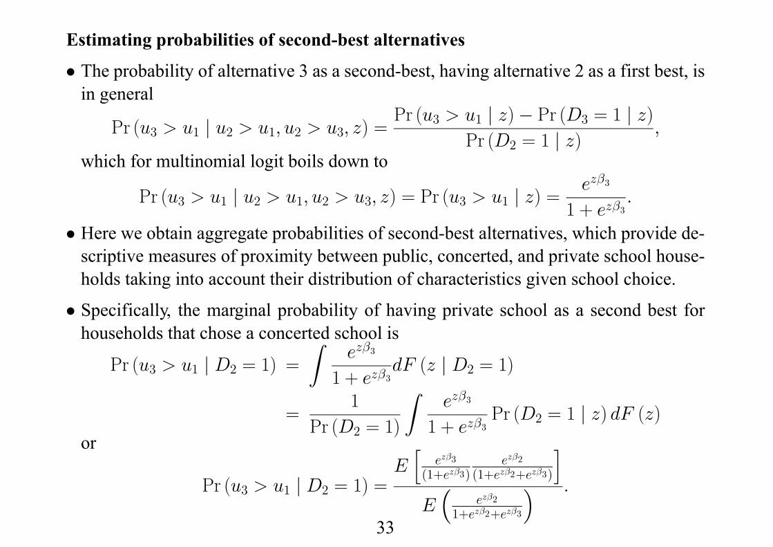
Estimating probabilities of second-best alternatives

• The probability of alternative 3 as a second-best, having alternative 2 as a first best, isin general

Pr (u3 > u1 | u2 > u1, u2 > u3, z) = Pr (u3 > u1 | z)− Pr (D3 = 1 | z)Pr (D2 = 1 | z) ,

which for multinomial logit boils down to

Pr (u3 > u1 | u2 > u1, u2 > u3, z) = Pr (u3 > u1 | z) = ezβ3

1 + ezβ3.

• Here we obtain aggregate probabilities of second-best alternatives, which provide de-scriptive measures of proximity between public, concerted, and private school house-holds taking into account their distribution of characteristics given school choice.

• Specifically, the marginal probability of having private school as a second best forhouseholds that chose a concerted school is

Pr (u3 > u1 | D2 = 1) =Z

ezβ3

1 + ezβ3dF (z | D2 = 1)

=1

Pr (D2 = 1)

Zezβ3

1 + ezβ3Pr (D2 = 1 | z) dF (z)

or

Pr (u3 > u1 | D2 = 1) =Eh

ezβ3(1+ezβ3)

ezβ2(1+ezβ2+ezβ3)

iE³

ezβ21+ezβ2+ezβ3

´ .

33

• In a partial equilibrium analysis that abstracts from externalities and public financeconsiderations, if Pr (u3 > u1 | D2 = 1) is close to , the subsidy implicit to the con-certed system does not create distortion because individual preferences are unaffectedby its introduction (under the assumption that private and concerted goods are similar).

• If Pr (u3 > u1 | D2 = 1) is close to 0, the subsidy creates a welfare loss, because aconcerted school is not preferable to public school in the absence of the subsidy.

• Table 9 reports estimated conditional probabilities of private school as a second-bestgiven concerted schooling as the first choice.

Table 9Probability of private school as second-bestgiven concerted school as first choiceSubpopulation %

< 100,000 inhabitants 3.1100,000 to 500,000 inhabitants 13.1> 500,000 inhabitants 12.5

All 8.7• The overall second-best probability is about four percentage points higher than themarginal probability of private school. Note the steep increase for large cities.

34

Summary of empirical results

1. The provincial income elasticity of the concerted/public odds ratio is 8 times largerthan the parental’s income elasticity, which suggests that community-level differencesin relative school quality or in effective choice opportunities matter more for schoolchoice than differences in individual income. This is not surprising given that manyconcerted schools are only marginally more expensive than public schools. Thisspeaks of the predominant role of residential location for school choice in Spain.

2. Parental education increases the preferences for non-public schools, but mother’seducation has a substantially stronger effect than father’s education.

3. Parents’ religiosity increases the preference for concerted schools other things equal.The concerted/public odds ratio of a religious household can be between 1.5 and 2times larger than the odds ratio of a non-religious one.

4. The gender of children also affects the preference for concerted schools. Theconcerted/public odds ratio of parents with a single daughter is 1.4 higher than theodds ratio of parents with a single son.

5. Choice of a public school in 1990 was more frequent in provinces with a largefraction of inter-regional immigrants, especially in those with a separate language.We interpret this effect as reflecting differences in choice opportunities amongimmigrants linked to residential location.

35

Conclusions

• We exploit partial information on individual school choices together with data onschooling expenditures to identify a multinomial model of the choice between pub-lic, concerted, and private schooling by Spanish parents in 1990.

• We find small but significant household income effects on school choice. Other de-terminants of school choice are the level of education of mothers and fathers, the reli-giosity of parents, and the gender of their children.

• A substantial part of variation in observed choices is due to area-wide variables suchas aggregate income, fraction of immigrants, or cultural diversity.

• Within our reduced formmodel we cannot separate aggregate effects due to differencesin relative quality of school type from effects due to differences in choice opportunities.

• But our results strongly hint that heterogeneity in the effective choice set are a signifi-cant part of the story, and that aggregate differences matter more for observed choicesthan individual differences in income or parental background.

• The fact that these effects are estimated on data collected prior to the wave of immi-gration of recent years would suggest the possibility of even stronger effects today.

• A comprehensive evaluation of concerted schooling in Spain will have to focus at themicro level on the distributions of schooling outcomes, such as test scores, and labourmarket outcomes, which at present we do not observe at household level.

36

Approximate multinomial initial estimates

• Preliminary estimates of themultinomial school choice and expenditure decisionswereused as initial values for the mixture likelihood estimation.

• We obtain them by assuming that only private-school parents with zero expenditures inregistration fees, are in concerted schools. They may be affected by misclassification.

• Tables C.1 and C.2 show the estimates. The main conclusions, related to the choice oftype of school are broadly similar to those obtained from the mixture model.

• But there are some differences in the relative magnitudes of household income effectsfor concerted and private schools, possibly reflecting biases due to misclassification.

• Comparison of the approximate classification with the mixture model classification:(a) Approximate classification: If (public=1) =⇒public; if (public=0 & registrationfees=0) =⇒ concerted; if (public=0 & registration fees>0) =⇒ private.

(b) Mixture-model classification: If (public=1) =⇒public; if (public=0 & registration+ tuition fees >0) =⇒ private or concerted; if (public=0, registration fees=0, &tuition fees =0) =⇒ concerted.

37

D Distribution of predicted probabilities

Table D.1 shows some descriptive statistics of the distributions of predicted

probabilities of the choice of public, concerted, and private schooling, which

are obtained from the ML estimates of the mixture model reported in Table

5. Table D.2 provides similar information for the approximate multinomial

estimates in the first two columns of Table C.1.

Table D.1Predicted probabilities

(Mixture model ML estimates)Public Concerted Private

Mean 0.77 0.21 0.03Min 0.05 0.004 0.00Max 0.996 0.83 0.63Q10 0.49 0.03 0.001Q25 0.67 0.08 0.002Q50 0.82 0.17 0.007Q75 0.92 0.30 0.02Q90 0.97 0.44 0.07

Table D.2Predicted probabilities

(Approximate logit estimates)Public Concerted Private

Mean 0.77 0.18 0.06Min 0.06 0.003 0.00Max 0.997 0.75 0.55Q10 0.49 0.03 0.004Q25 0.67 0.06 0.01Q50 0.82 0.14 0.04Q75 0.92 0.25 0.08Q90 0.97 0.39 0.13

The average proportion of private schools in Table D.1 is similar to the

aggregate 1990 figure known from other sources, but the proportion of con-

certed schools is too small. This may be due to stratification in the EPF or

to misclassification error in the EPF public/non-public indicator.

36