Water Quality Management in Rivers using Water Quality Models for Assessment and Prediction

Sudhira H. S.1, Praveen Gurukar S.2, Anurita3 and Lokesh K. S.4

1 Energy and Wetland Research Group, Centre for Ecological Sciences, Indian Institute of Science, Bangalore –560 0122 JSS Consultants, SJCE Campus, Manasagangothri, Mysore – 570 0063 Aspire Communications, SJCE Campus, Manasagangothri, Mysore – 570 0064 Department of Environmental Engineering, Sri Jayachamarajendra College of Engineering, Mysore – 570 006. Karnataka. India.

Water quality assessment in rivers has attained considerable importance in recent years. This is because of the deterioration of river water quality due to pollution from different sources attributed to human activities on the pretext of economic development. Water quality modeling and subsequent prediction can be one of the most important potential tools for water quality management in rivers. In this regard, the current paper highlights the importance of water quality assessments in rivers with a thrust on management.

This paper presents a study on water quality assessment and modeling studies undertaken for river Cauvery at Srirangapatna. The water sampling was done at six transects along the river stretch over a distance of 5 km. Water quality monitoring was done over a period of three months extending from February 2002 to April 2002. The water quality parameters and upstream flow characteristics were analyzed for review and validation of available water quality model under steady-state conditions.

Water quality model developed by Gurudatt (1989) was applied in the present study. In particular the model MIXPIPOX for single effluent discharge is used here. The river water quality and hydrological characteristics were used as inputs for this program. The low river flow analysis was also carried to determine the design flow for the least flow in the river representing the critical flow conditions. These data were further used to calibrate and validate the MIXPIPOX computer model for the conditions prevailing in the river. The non-dimensional diffusion factor value ( was arrived at by using the conservative parameters (conductivity, TDS) for model calibration and validation was done using non-conservative parameter (BOD).

The decay rates, reaeration coefficients and values for each transect was used to compare the observed and predicted values by plotting graphs for the same. From these plots, it was found that observed and predicted values correlate well for three transects and agree with the trend for the rest of the transects. Finally, the study evaluated the viable engineering option of setting up effluent treatment plant for river Cauvery near Srirangapatna considering the rates, decay rates and reaeration coefficients. This was carried for the options of providing primary and secondary treatments only. From the water quality assessments the extent of pollution in the river is not very significant. The paper discusses some aspects accounting for this phenomenon as well as other options available for safe and efficient disposal of wastewaters.

Introduction

Environmental pollution control has evolved as one of the major themes among decision makers and planners, while posing a greater challenge to engineers and scientists to understand and analyze various phenomena involving this. In general it is hard to define and quantify many of the important physical, chemical, biological, economic and social interrelationships, between the many components of any environmental pollution control system. Constraints in manpower, technical know-how and economic resources have led to lesser understanding of such systems.

River systems are subjected to undue pollution loading in the form of industrial and domestic discharges. Prevention and control of pollution to rivers in India often follow the obsolete “end-of-pipe” treatment methods. In order to assess the impacts of wastewater discharge on the receiving water body’s quality, computer aided mathematical models, once calibrated for existing river quality conditions can be used to generate future scenarios of water quality due to increased pollution loads, and also simulate alternative wastewater treatment scenarios, thus forming an integral part of the decision making system for water quality management.

Water quality models are thus evolved in order to predict and assess various conditions that may prevail in the water body due to effluent discharges. Water quality models are mathematical constructs, which integrate a number of complex phenomena such as water transport, reaction kinetics, and external loadings. There are two basic reasons for constructing mathematical representations of natural aquatic ecosystems. First, there is a need to increase the current level of understanding regarding the cause-effect relationships operative in all aquatic environments. Secondly, models provide a synthesis of understanding, which is increasing in the policy arena. Mathematical models, which incorporate the characteristics of river channel, outfall and pollutants of concern, are utilized as tools in such analyses.

Water quality simulation models are used extensively in waste load allocation studies, environmental impact investigations and for analyzing the cause and effect relationships in a water body. A common feature in most of these models is the use of rate parameters to describe processes occurring in the water body. The reliability of the model is a function of, among other things, how well these parameters reflect the processes they are intended to describe.

The processes involved in modeling are model calibration, model verification, model application and model post audit. Calibration is the process of identifying appropriate values for model parameters and is a difficult task because of uncertainty in the mathematical expression of the system (model structure identification), the inability to control environmental experiments, and uncertainty in field data (Beck 1983). The expert system or the expert advisor projects undertaken by the Environmental Protection Agency (EPA) at the Center of Exposure Assessment Modeling recognized calibration as the single most difficult step in modeling water quality.

Models of water quality have evolved over the course of time in response to various issues. This evolution has included increased complexity in the number of aquatic processes that have been included like – nitrogen and phosphorus cycling and interaction with primary and secondary trophic levels, toxic chemical fate and transport processes of solids partitioning and biodegradation and volatilization, and aquatic food web chemical bioaccumulation models. But there has been more significant development over time that has resulted from the management issues of controllability. From the perspective of the need to incorporate external causative inputs into the overall modeling framework, three different stages of water quality modeling are identified (Thomann, 1998).

One Dimensional DO Modeling in RiversDissolved Oxygen (DO) is an important water quality parameter affecting the health of a river and hence, great deal of importance is attached to maintain the DO at desirable level. DO is important to aquatic life because detrimental effects can occur when DO levels drop below 4 mg/L or 5 mg/L, depending on the aquatic species. Suspended solids influence the water column turbidity and ultimately settle at the bottom, leading to possible benthic enrichment, toxicity and sediment oxygen demand. Nutrients can lead to eutrophication and DO depletion. Thus, in order to evaluate the effects of wastewater discharge on instream DO level, it is necessary to understand the relationship between pollutant characteristics and stream environment.

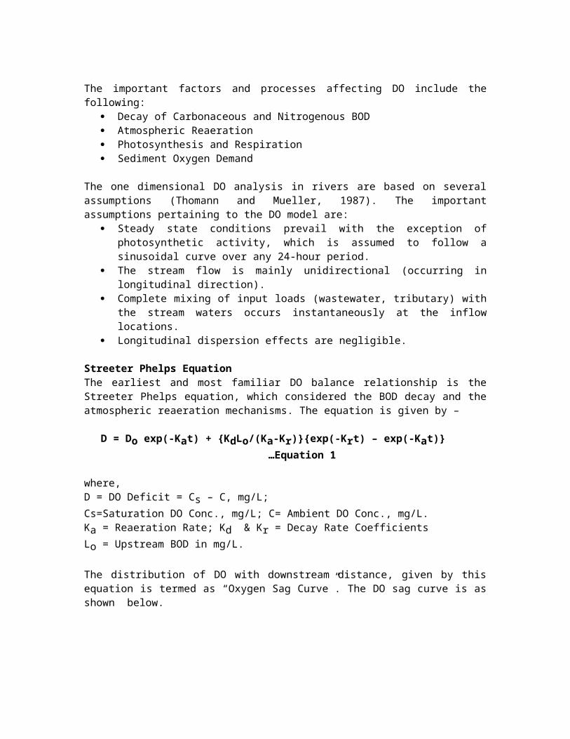
The important factors and processes affecting DO include the following: Decay of Carbonaceous and Nitrogenous BOD Atmospheric Reaeration Photosynthesis and Respiration Sediment Oxygen Demand

The one dimensional DO analysis in rivers are based on several assumptions (Thomann and Mueller, 1987). The important assumptions pertaining to the DO model are:

Steady state conditions prevail with the exception of photosynthetic activity, which is assumed to follow a sinusoidal curve over any 24-hour period.

The stream flow is mainly unidirectional (occurring in longitudinal direction). Complete mixing of input loads (wastewater, tributary) with the stream waters occurs

instantaneously at the inflow locations. Longitudinal dispersion effects are negligible.

Streeter Phelps EquationThe earliest and most familiar DO balance relationship is the Streeter Phelps equation, which considered the BOD decay and the atmospheric reaeration mechanisms. The equation is given by –

D = Do exp(-Kat) + {KdLo/(Ka-Kr)}{exp(-Krt) – exp(-Kat)} …Equation 1

where,D = DO Deficit = Cs – C, mg/L;Cs=Saturation DO Conc., mg/L; C= Ambient DO Conc., mg/L.Ka = Reaeration Rate; Kd & Kr = Decay Rate CoefficientsLo = Upstream BOD in mg/L.

The distribution of DO with downstream distance, given by this equation is termed as “Oxygen Sag Curve”. The DO sag curve is as shown below.

Figure 1: Dissolved Oxygen Sag Curve

It is seen that the DO concentration, C, reaches a minimum at a location termed as critical location. At this point, oxygen uptake by BOD is just balanced by the oxygen input from the atmosphere.

Generalized Steady State ModelAs outlined by Thomann and Mueller (1987), the DO balance equation can be written as follows for steady state conditions by using the daily average photosynthetic rate, P av (instead of the diurnal DO variation):

dD/dt = KdL + KnN – KaD – Pav + R + Sv …Equation 2

However over the years analysts have used the general steady state model for water quality modeling studies using computer programs for analysis.

Computer Programs for Water Quality ModelingComputer programs have been developed to aid in the data analysis, and for model validation and application to evaluate viable engineering and management options. The programs written in FORTRAN include algorithms to consider the effect of background concentration of pollutants. These are based on the concept of mixing zones in rivers and methods developed by Gowda (1980, 1984a and 1984b). The program MIXPIPOX has been developed to simulate the lateral and longitudinal distributions of CBOD and DO in river channels receiving effluents from pipe out fall at bank or in river channel (Gurudatt, 1989). There is only one outfall in the study stretch of the river and hence, the computer program MIXPIPOX applicable to DO evaluation in rivers having single outfall is utilized for the DO model evaluation.

ObjectivesThis paper brings out the study to assess the quality of river water and quantitatively predict the effect of polluting discharges on river quality by evaluating the existing model using field data. This paper explores the application of MIXPIPOX model for predicting DO in river Cauvery, at Srirangapatna where the river is polluted by domestic wastewater from a pipe outfall. The specific objectives of the study were:

TRAVEL TIME

Saturation DOD

O

CRITICAL POINT

To monitor and evaluate river water quality due to effluent discharges into river Cauvery at Srirangapatna.

Low flow analysis for the design conditions. Review and validation of available water quality models under steady-state conditions. To calibrate and validate the model using field data. To apply the model for evaluating viable engineering options.

River Cauvery is an important source for agriculture, drinking water supply and other purposes. For the present study river Cauvery was chosen near Srirangapatna town, since at present there is no wastewater treatment facility in this town. The domestic wastewater is directly discharged into the river, due to which the river water is experiencing significant pollution.. Hence, the stretch of river Cauvery near Srirangapatna town has been selected for a detailed water quality assessment and modeling studies.

Description of Study AreaThe domestic wastewater from the Srirangapatna is discharged into the River Cauvery. Srirangapatna is an island formed by the branches of river Cauvery. The geographical location of Srirangapatna is 76o 41’ longitude and 12o15’ latitude. The Sriranganatha temple and Nimishamba temple are located on the banks of this river. This attracts lot of tourist all round the year and hence there is a high floating population. There is a Bathing Ghat close to the Sriranganatha temple at the north branch of the river. The sewage effluent of the town is also let into north branch of the river. Further, downstream of the river, due to the presence of Bathing Ghat close to the famous Nimishamba temple, the river is again subjected to contamination. The study stretch of the river is shown in Figure 2. This necessitated a detailed water quality evaluation both upstream and downstream of the river for an assessment and model application.

The sampling sites were selected considering the following points: Objectives of the study Sources of pollution Physical characteristics of the stream Accessibility of the site Equipment availability

Water sampling was therefore done at upstream and downstream of bathing ghats and at various places along the river until the two branches of river confluences at Sangam. The water quality parameters (DO, BOD, Chlorides, pH, Temperature, Specific Conductivity) and upstream flow characteristics were all analyzed for review and validation of available water quality models under steady state conditions. These data were also used to calibrate and validate the model for the conditions prevailing in the river.

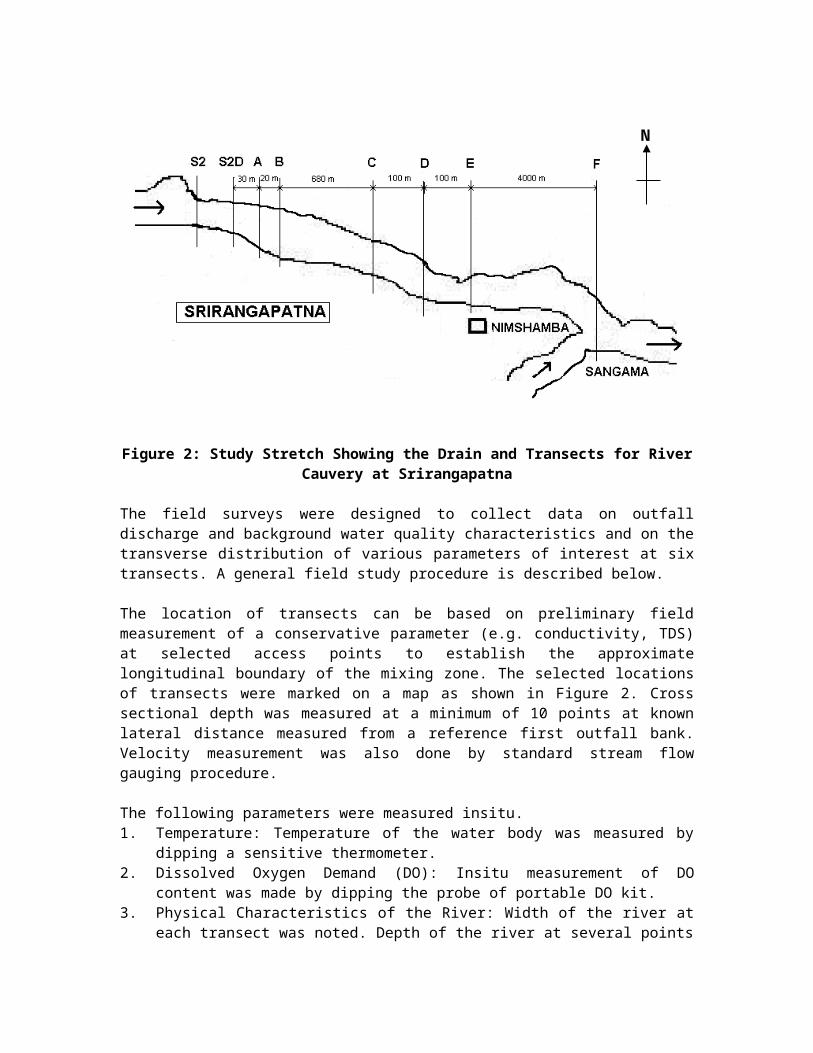
Figure 2: Study Stretch Showing the Drain and Transects for River Cauvery at Srirangapatna

The field surveys were designed to collect data on outfall discharge and background water quality characteristics and on the transverse distribution of various parameters of interest at six transects. A general field study procedure is described below.

The location of transects can be based on preliminary field measurement of a conservative parameter (e.g. conductivity, TDS) at selected access points to establish the approximate longitudinal boundary of the mixing zone. The selected locations of transects were marked on a map as shown in Figure 2. Cross sectional depth was measured at a minimum of 10 points at known lateral distance measured from a reference first outfall bank. Velocity measurement was also done by standard stream flow gauging procedure.

The following parameters were measured insitu.1. Temperature: Temperature of the water body was measured by dipping a sensitive

thermometer.2. Dissolved Oxygen Demand (DO): Insitu measurement of DO content was made by dipping

the probe of portable DO kit.3. Physical Characteristics of the River: Width of the river at each transect was noted. Depth

of the river at several points along individual transect was measured by dipping a graduated rod while traveling on a raft. Velocity of the flow in the river was measured using a rubber ball as a float, which was allowed to float between two points in the river. The distance between the two points and time of travel of the ball were recorded and the velocity of flow was calculated. Average velocity was determined by repeating the process two to three times.

4. Wastewater Flow: The flow of wastewater that enters the river from the Srirangapatna town was measured.

5. River Water Flow: Flow of river Cauvery during the study period was noted from the records of National River and Lake Conservation Directorate (NRLCD).

N

The geometric and hydraulic data are given in Table 1. The water samples transported to the laboratory were analyzed according to the procedures given in Standard Methods (1992) as mentioned below:i. pH – Measured using a digital pH meter

ii. Conductivity – Measured using a digital conductivity meteriii. TDS – Measured by digital TDS meteriv. BOD – By standard dilution techniquev. COD – Reflux method

The observed water quality data for the month of April 2002 are presented in Table 2.

Table 1: Geometric and Hydraulic Data of Study Stretch of Cauvery RiverTransects A B C D E F

Distance ‘x’ meters 50 80 730 830 930 4930Discharge in m3/sec 70.54 70.54 70.54 70.54 70.54 70.54

Upstream River Flow m3/sec 72.48 72.48 72.48 72.48 72.48 72.48

Effluent Flow Rate m3/sec 0.06 0.06 0.06 0.06 0.06 0.06

Width ‘b’ meters 75 80 65 65 95 80Depth ‘h’ meters 0.5 0.45 0.65 0.60 1.29 0.85

Velocity ‘v’ m/sec 0.42 0.40 0.38 0.40 0.5 0.75

Table 2: Water Quality Parameters of Cauvery River for the month of April 2002

Details DistanceIn meters

Temperature o

C pH DOmg/L

TDSmg/L

CODmg/L

BODmg/L

Conductivity mhos/cm

Effluent Discharge - 28.9 6.9 2.5 320 60.8 18.0 662

Upstream - 27.9 7.6 7.47 190 12.8 1.4 432Transect A 50 28.0 7.3 3.28 250 40.6 16.7 535Transect B 80 28.0 7.2 4.67 240 23.8 12.3 520Transect C 730 28.2 7.6 7.2 210 15.7 3.6 463Transect D 830 28.0 7.5 7.4 220 30.2 2.3 456Transect E 930 28.2 7.6 7.2 220 28.0 1.0 452Transect F 4930 28.4 7.8 6.8 210 19.2 1.4 452

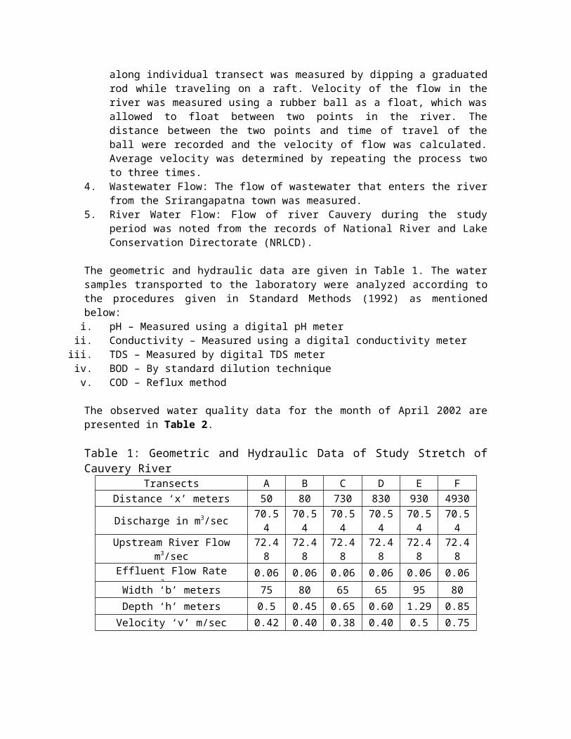
Stream Flow AnalysisChanges in water quality parameters and the assimilative capacity of a river are essentially dependent on the flow of the river at any given time. Critical water quality condition occurs during low flow periods. The low river flow analysis was carried to determine the design flow for the least flow in the river representing the critical flow conditions. This critical flow is used to determine the impact of wastewater on the river. Hence, it is essential to conduct a stream flow analysis exercise to determine the minimum flow of the river. The average minimum flows in the River Cauvery during 2001-2002 are presented in Table 3. In the present study the most critical flow conditions were determined by subjecting the average minimum flows over the period mentioned above to probability analysis. The data were arranged

in ascending order and ranked. The probability of occurrence of each flow (p) was determined from:

P = m/(n+1) …Equation 3

where; ‘m’ is the rank of each flow and n is the total number of observations. The values of probability (p) were plotted against the corresponding values of discharge (Q), shown in Figure 3. From this plot, the flow with 90% probability of occurrence was obtained to be 72.48 cumecs just upstream of the effluent outfall. This represents the low flow in Cauvery river at Srirangapatna. In this study, flow increase due to seepage from the catchment area is ignored which means that the low flow considered will be a conservative estimate.

Table 3: Analysis of Flow Data of River Cauvery

Month Average Minimum Flows Rank P = m/(n+1) * 100

(%)February 5.47 1 7.69March 18.23 2 15.38April 17.59 3 23.08May 22.77 4 30.77June - 5 38.46July - 6 46.15August - 7 53.85September - 8 61.54October 44.52 9 69.23November 50.00 10 76.92December 68.07 11 84.61January 52.87 12 92.30

Model Validation for Conductivity and TDSThe validation of the MIXPIPOX model has been carried out in two steps. In the first step, the model was calibrated using the data on conservative pollutants to obtain . The observed conductivity distributions exhibited the characteristics of a shore attached plume. The distribution data were used to calibrate the model applicable to conservative material from which the values are determined for each transects. The procedure is outlined below.

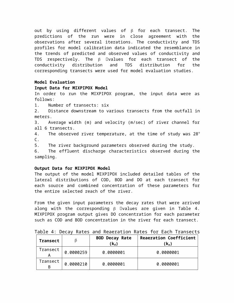
The input data for the model calibration of MIXPIPOX model were obtained from the observed data shown in Table 1 and Table 2. The upstream river discharge of 72.48 m3/sec before Transect - A and the wastewater discharge of 0.06 m3/sec, along with the conductivity concentration of 662 mhos/cm and TDS concentration of 320 mg/L in the domestic wastewater were considered as inputs. Using these the concentration distributions of conductivity and TDS at various transects was predicted. Several runs were carried out by using different values of for each transect. The predictions of the run were in close agreement with the observations after several iterations. The conductivity and TDS profiles for model calibration data indicated the resemblance in the trends of predicted and observed values of conductivity and TDS respectively. The values for each transect of the conductivity distribution and TDS distribution for the corresponding transects were used for model evaluation studies.

Model Evaluation

Input Data for MIXPIPOX ModelIn order to run the MIXPIPOX program, the input data were as follows:1. Number of transects: six2. Distance downstream to various transects from the outfall in meters.3. Average width (m) and velocity (m/sec) of river channel for all 6 transects.4. The observed river temperature, at the time of study was 28o C.5. The river background parameters observed during the study.6. The effluent discharge characteristics observed during the sampling.

Output Data for MIXPIPOX ModelThe output of the model MIXPIPOX included detailed tables of the lateral distributions of COD, BOD and DO at each transect for each source and combined concentration of these parameters for the entire selected reach of the river.

From the given input parameters the decay rates that were arrived along with the corresponding values are given in Table 4. MIXPIPOX program output gives DO concentration for each parameter such as COD and BOD concentration in the river for each transect.

Table 4: Decay Rates and Reaeration Rates for Each TransectsTransect BOD Decay Rate (kd) Reaeration Coefficient (ka)

Transect A 0.0000259 0.0000001 0.0000001Transect B 0.0000210 0.0000001 0.0000001Transect C 0.0000148 0.0000001 0.0000003Transect D 0.0000190 0.0000001 0.0000008Transect E 0.0000230 0.0500000 0.0000003Transect F 0.0000091 0.0003200 0.0000004

The observed BOD concentrations were compared with the BOD concentrations predicted from the MIXPIPOX program. It was observed from the first and second transects that the observed values of BOD were higher than the predicted values. This was due to the stagnation of water at the bank, while there was relatively greater flow at the center of the river. Further, the observed and predicted value correlated well for subsequent lateral points in both these transects. The observed and the predicted BOD concentrations for all transects were compared with values, decay rates and reaeration coefficients as shown in Table 4.

Similarly, the observed COD concentrations were compared with the COD concentrations predicted from the MIXPIPOX program. The observed and the predicted BOD concentrations for all transects correlated well with values, decay rates and reaeration coefficients as shown in Table 4.

The DO profiles were also plotted (Figure 4) from the values obtained from the MIXPIPOX program for the parameter BOD. It can be observed from the Figure 4, the DO profiles for various transect. The DO drops after the confluence of the domestic wastewater and subsequently increases over the stretch within a distance of 250 meters. However, it is also seen that there is variation in the DO profile significantly in the later transects. This is due to presence of Dhobi Ghats at Transects B, C and D Bathing Ghat at Transect E and F.

Figure 4: DO Profile for the Study Stretch

MIXPIPOX Model ApplicationThe main intent of the modeling study was to utilize the model to evaluate potential impacts of any viable engineering options such as provision of a treatment plant. In line with this need, the application of the calibrated MIXPIPOX model to assess the probable impacts of provision of different stages of treatment was evaluated.

The options considered for assessment using the MIXPIPOX program model for the case study of River Cauvery near Srirangapatna were as follows:

o Upstream flow in the river just above the first outfall – For this analysis, the flow with 90 % of the probability of occurrence in the lean flow was selected for analysis.

o Wastewater Treatment Options – Discharge of wastewater into the river without any treatment Discharge of effluent with primary treatment Discharge of effluent with secondary treatment

Evaluation of OptionsMIXPIPOX program was applied to predict the DO profiles for specified lateral boundary of the mixing zone and for various options stated earlier such as the raw effluent, primary treated effluent and secondary treated effluent entering the river. The predictions were used to find a minimum DO level for each option and its location.

For evaluating the options, the percentage removal of BOD for primary treatment is 35 % and for secondary treatment 70 % was considered. The DO profiles for various options at 10 % lateral boundary are shown in Figure 5. From the figure the minimum DO is at 30 m downstream of outfall being 6.54 mg/L and the highest 7.32 mg/L at 4000 m downstream of outfall. This indicated that there is no critical DO concentration zone in the study stretch.

It was seen from the figure that the initial upstream DO concentration of 7.5 mg/L drops after the domestic wastewaters discharge into the river. The behaviour of DO without treatment for the raw effluent is shown in Figure 4. The DO profiles for the effluent after primary and secondary treatment also follow the same trend. However, it can be inferred that by providing the primary and secondary treatment the DO values downstream increases marginally.

0 1000 2000 3000 4000 50006.0

6.5

7.0

7.5

8.0

WITHOUT TREATMENT WITH PRIMARY TREATMENT WITH SECONDARY TREATMENT

DO

CO

NC

ENTR

ATIO

N IN

mg/

L

DISTANCE FROM OUTFALL IN METERS

Figure 5: DO Predictions at the Bank for Different Treatment Options

Summary and ConclusionsThis study deals with the application of MIXPIPOX computer model to predict the DO concentrations in mixing zones of rivers receiving single effluent pipe outfall. The study area is the River Cauvery at Srirangapatna in Karnataka. The river here has the domestic wastewater effluent discharged into the river.

The field data were collected at six transects in the above river segment length of 4.93 km. The computer program MIXPIPOX has been used to analyze the field data. The non-dimensional diffusion factor was arrived at using the conservative parameters (conductivity, TDS). The reaeration rates and decay constant for the non-conservative substance, BOD were then arrived using the model.

A calibration study of MIXPIPOX model was conducted (by trial and error) to get reasonable agreement between the predicted and observed DO by adjusting the decay rates and reaeration coefficient. The calibrated model was used to predict the minimum DO concentration and its location, for raw, primary treated and secondary treated effluent discharge. From this, the most suitable type of treatment facility to be provided is secondary treatment.

ConclusionsThe following conclusions were drawn out of the study. The effluent discharge from the outfall was found to create lateral concentration gradient thus forming a zone of incomplete lateral mixing (i.e. mixing zone) in river Cauvery at Srirangapatna. From the calibration of water quality model MIXPIPOX the process parameters were estimated for the study segment of the river. The observed and predicted values correlate well with three transects and agree with the trend for the rest of the transects. The low flow in the river was found to occur during the month of April and the 90% of the probable flow was estimated to be 70.48 m3/sec. From the study it was found that by providing the primary and secondary treatment the DO values downstream increase marginally. By providing the treatment, apart from the DO values, the other characteristics of the river like TDS, conductivity, COD are all significantly reduced. It is essential to provide the treatment, as there is significant human activity along the downstream of the river.

Thus the study demonstrated the application of water quality models in assessment and prediction in rivers that would of immense help in the water quality management in rivers especially for decision makers and water quality engineers; as well scientists and students can use the models to study these under different conditions.

REFERENCES

1. Beck, M.B., (1983). “Uncertainty, System Identification, and the Prediction of Water Quality”, Uncertainty and Forecasting of Water Quality, M.B. Beck and G. van Straten, eds., Springer-Verlag, Berlin, Germany.

2. Gowda, T.P.H., (1980). “Stream Tube Model for Water Quality Prediction in Mixing Zones of Shallow Rivers“, Water Resource Paper 14, Water Resources Branch, Ontario Ministry of Environment, Toronto, Canada.

3. Gowda, T.P.H., (1984a). “Critical Point Method for Mixing Zones in Rivers”, ASCE, Journal of Environmental Engineering, Vol. 110, No. 1, pp 244-262.

4. Gowda, T.P.H., (1984b). “Water Quality Predictions in Mixing Zones in Rivers”, ASCE, Journal of Environmental Engineering, Vol. 110, No. 4, pp 751-769.

5. Gurudatt, R., (1989). M. Tech Thesis, Sri Jayachamarajendra College of Engineering, Mysore.

6. NEERI, (1988). “Manual on Water and Wastewater Analysis”, NEERI, Nagpur, India.7. “Standard Methods for the Examination of Water and Wastewater“, (1995). 19th ed.

American Public Health Association, American Water Works Association, and Water Pollution Control Federation, American Public Health Association, Washington, DC.

8. Thomann, R.V., (1998). “The Future “Golden Age” of Predictive Models for Surface Water Quality and Ecosystem Management”, ASCE, Journal of Environmental Engineering, Vol. 124, No. 2, pp 94-103.

9. Thomann, R.V., and Mueller, J.A., (1987). “Principles of Surface Water Quality Modeling and Control”, Harper & Row Publishers, N.Y., U.S.A.