inundation mapping and hydraulic reconstructions of an...

Inundation Mapping and Hydraulic

Reconstructions of an Extreme Alluvial Fan

Flood, Wild Burro Wash, Pima County,

Southern Arizona

Arizona Geological Survey

Open-File Report 04-04

Kirk R. Vincent1, 2

, Philip A. Pearthree 1, P. Kyle House

1, 3,

and Karen A. Demsey1, 4

December, 2004

1 all authors are current or former employees of the Arizona Geological Survey

2 U.S. Geological Survey, 3215 Marine Street, Boulder, Colorado 80303

3Nevada Bureau of Mines and Geology, University of Nevada, Reno, Nevada 89557

43055 NE Everett St., Portland, Oregon 97232

This research was supported by the Pima County Flood Control District,the National Science Foundation, the Arizona Geological Survey, and

the U.S. Geological Survey

i

CONTENTS

Abstract ......................................................................................................................................1

Introduction ................................................................................................................................2

Background...........................................................................................................................3

Wild Burro Fan in the Spectrum of Alluvial Fans..................................................................5

Scope and Organization of Report .........................................................................................6

Definitions of Important Terms .............................................................................................6

Site Description and Geologic History ........................................................................................8

Piedmont Geomorphology.....................................................................................................9

Wild Burro Fan ...................................................................................................................10

Storm Event and Flood Size......................................................................................................13

Flood Inundation Mapping Methods and Limitations ................................................................14

Flood Inundation Patterns .........................................................................................................20

General Distribution of Flow...............................................................................................20

Influence of Roads ..............................................................................................................21

Expansion/Contraction Channel Geometry..........................................................................22

Downstream Patterns of Flow in the Distributary Network..................................................23

Hydrology of the Distributary Network ...............................................................................27

Inundation of Landforms of Differing Age ..........................................................................28

Sediment Erosion and Deposition .............................................................................................28

Changes in the Distributary Channel Network.....................................................................28

Bank Erosion ......................................................................................................................30

Bed Scour and Backfill .......................................................................................................31

Hydraulic Reconstruction and Hydraulic Geometry ..................................................................36

Hydraulic Reconstruction Methods and Uncertainties .........................................................36

Hydraulic Modeling Results ................................................................................................41

Implications for Piedmont Flood-Hazard Assessment ...............................................................45

Acknowledgments ....................................................................................................................47

References ................................................................................................................................47

Figures

1. Map showing location of Wild Burro fan in southern Arizona ..........................................2

2. Map showing maximum extent and depths of inundation for the 1988 Wild Burro flood,Wild Burro Wash, southern Arizona ...............................................................................4

3. Diagram showing geomorphic features of desert piedmonts within tectonically inactive

Basin and Range landscapes ............................................................................................7

4. Map showing surficial geologic deposits for part of the southern Tortolita piedmont withoverlay of the 1988 flood inundation map........................................................................9

5. Graph showing surveyed longitudinal profile of Wild Burro fan following the main wash

along the length of the flood inundation map ................................................................13

6. Map showing dirt roads and their influence on flow during the 1988 flood ......................22

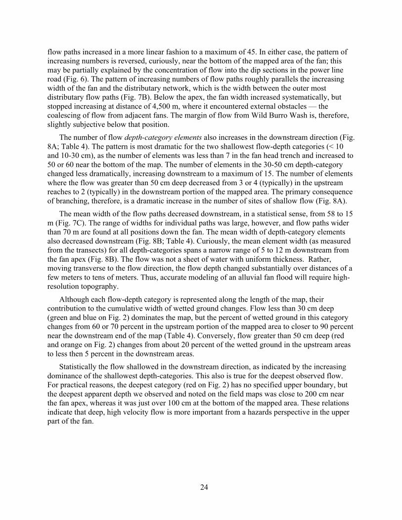
7. Graphs showing flow path characteristics in relation to distance downstream ..................25

ii

8. Graphs showing depth-category element characteristics in relation to distance downstream......................................................................................................................................26

9. Aerial photographs showing Wild Burro alluvial fan before and after the July 27,1988

flood..............................................................................................................................29

10. Graph showing example of a channel cross-section used in hydraulic modeling of peak

flow in narrow reaches for the 1988 flood, including the scour limit and backfill sediment

......................................................................................................................................32

11. Graph showing relation of apparent flow depth and streambed sediment backfill thickness......................................................................................................................................33

12. Graphs showing examples of longitudinal profiles used to model 1988 flow hydraulics in

narrow reaches ..............................................................................................................38

13. Graphs showing downstream hydraulic geometry relations for discharge and width inchannels, for Wild Burro flood in comparison with that from other areas.......................43

14. Graphs showing downstream hydraulic geometry relations for discharge and flow width,

depth, and velocity in channels for Wild Burro Wash, compared to assumptions in amodel used to assess flood hazards on fans ...................................................................44

Tables (in manuscript and on CD in the map pocket of this report)

1. Size of bed sediment along the main channel of Wild Burro Wash .................................11

2. Areas of inundation organized by flow depth category and landform type, based on GIS

analysis of the rectified flood inundation map ...............................................................16

3. Downstream patterns of widths and numbers of flow paths for 1988 Wild Burro flood ...18

4. Downstream patterns of widths and numbers of depth-category elements, excluding on-fanrunoff channels, for 1988 Wild Burro flood...................................................................19

5. Thickness of streambed backfill sediment in select narrow channels ...............................34

6. Measurements and observations of flow-roughness values, flow velocity, and Froude

number for flow in desert streams with fine-grained beds ..............................................37

7. Selected hydraulic parameters derived from modeling peak flow for the 1988 floodthrough narrow reaches of all sizes on Wild Burro fan...................................................40

Plates (digital maps and GIS databases on CD in the map pocket of this report)

1. Digital version of inundation map for the 1988 Wild Burro flood.

2. Digital version of map of surficial geologic deposits within and near the Wild Burro fan.

1

ABSTRACT

In the evening of July 27, 1988, an extreme flood inundated the channels and floodplain of a

relatively pristine, undeveloped alluvial fan associated with Wild Burro Wash, located on a

desert piedmont near Tucson, Arizona. Subsequently, we spent about 200 person-days in the

field mapping in detail the distribution of flooding on the fan, differentiating flow into several

depth classes over an area of 4.4 km2 and collecting data to reconstruct the peak-flow hydraulics

in select narrow reaches. The results of that effort are described herein.

The flood was the result of an intense thunderstorm, centered over a small (23 km2) bedrock

watershed. This was a sediment-laden water flood (not a debris flow) that was conveyed in

distributary (downstream-branching), hydraulically steep (0.026-0.029 m/m) sand-bedded

channels and over extensive floodplain areas.

The flood inundated about half of the fan area. About 35 percent of the flooded area

consisted of flow in channels, and the remainder was flow on the vegetated floodplain. Most (81

percent) of the inundated area was covered by water less than 30 cm deep at peak flow, on the

floodplain and in small channels. Deeper flow (as much as 200 cm) occurred predominantly in

larger channels. The flow repeatedly branched downstream, and occasionally reconverged. As a

result the number of flow paths increased downstream, from 1 to 4 near and upstream from the

fan apex to a maximum of 45 flow paths 3.5 km downstream from the apex. The width and depth

of flow paths decreased downstream, statistically, but channels containing deep and swift flow

occurred at all positions on the fan. The areas of ground not flooded were narrow, typically less

than 30 m wide (perpendicular to flow direction) irrespective of position on the fan.

Channels on the Wild Burro fan exhibit a striking geometry marked by spatially repetitive

variation in width, depth, and bed gradient. The pattern consists of narrow-reaches that are deep

and have distinct channel banks, alternating with expansion-reaches that are wide and shallow

and have low or indistinct banks. The longitudinal bed-profiles are concave-up in the narrow

reaches and are convex-up in the expansion reaches. This pattern is evident over a large range in

channel size (bankfull discharge). The expansion/contraction pattern is an integral part of the

distributary network, in that the flow branches only at expansion reaches.

Flow reconstruction indicates that the discharge at the fan apex was extreme (200-300 m3/s),

considering the size of the watershed, and the flow was swift. Upon entering the narrow reaches,

increasing gradient and channel narrowing caused the flow to accelerate and deepen, become

supercritical, and scour. Upon entering the expansion reaches, decreasing gradient and channel

widening caused the flow to decelerate and shallow, become subcritical and presumably deposit

sediment, and flow overbank or into multiple distributary channels.

The Wild Burro flood passed through preexisting channels that were uniquely suited to

convey the flow. Most channel banks were trimmed, but none by very much, and no large

channels were newly formed. This suggests an equilibrium of form and process, such as exists

for meandering streams, but in this case the flows that act to construct and maintain the channels

of the distributary network are infrequent with recurrence interval of many decades.

The results of this study provide insight into issues important to geomorphology including

spatial patterns of ephemeral distributary flow, the hydraulics and hydraulic geometry of

channels on alluvial fans dominated by water floods, and the magnitude and frequency of events

2

in relation to their efficacy in shaping the landscape. In addition, the results provide important

information for models aimed at assessing flood hazards on alluvial fans.

INTRODUCTION

This report describes our study of an extreme flood that inundated the channels and

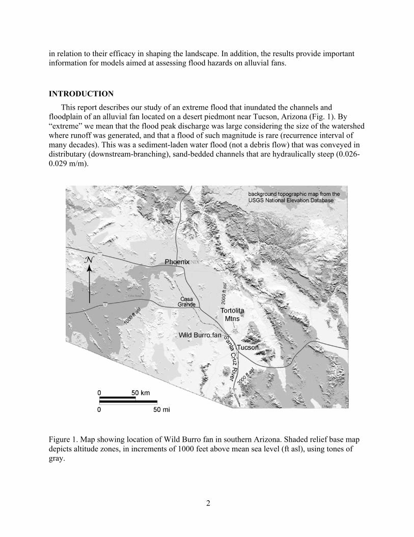
floodplain of an alluvial fan located on a desert piedmont near Tucson, Arizona (Fig. 1). By

“extreme” we mean that the flood peak discharge was large considering the size of the watershed

where runoff was generated, and that a flood of such magnitude is rare (recurrence interval of

many decades). This was a sediment-laden water flood (not a debris flow) that was conveyed in

distributary (downstream-branching), sand-bedded channels that are hydraulically steep (0.026-

0.029 m/m).

Figure 1. Map showing location of Wild Burro fan in southern Arizona. Shaded relief base map

depicts altitude zones, in increments of 1000 feet above mean sea level (ft asl), using tones of

gray.

3

Background

Flash floods on desert piedmonts are worthy of study because they shape the modern

landscape and can pose a significant hazard to people and property. Desert piedmonts extend

over huge areas, covering roughly half the area of nine states in the western United States and

northern Mexico, for example. Although extreme flooding at any individual site is rare, flooding

of ephemeral washes (channels) is common on a regional basis because of the large number of

such washes. Within the 140,000 km2 Basin and Range physiographic province of Arizona there

are approximately 5,000 small (~5 to 100 km2), mountainous watersheds draining into wash

networks on alluvial piedmonts. Thousands of flow events occur within this region during most

years, and statistically 100-year flood discharges are equaled or exceeded in 50 wash networks

each year. Floods have shaped the modern landscape on desert piedmonts (Bull, 1991), are an

important ecological factor affecting the distribution of plants and animals in the desert

(McAuliffe, 1994), and may act to recharge groundwater. These floods also pose a significant

hazard to people and property as urban areas rapidly expand onto desert piedmonts (French,

1987; National Research Council, 1996).

Floods of the type we describe are not well studied largely because of the complex nature of

the processes and the widespread distribution of flow. As noted above, washes on arid alluvial

fans are almost always dry, and large flows are rare at any one site. When flooding does occur

the durations of flow are brief and discharges change rapidly. Peak discharges also change

spatially, as water may occupy multiple distributary channels, may cover wide areas of

floodplain between washes, and may locally reconverge. In addition, the bed and banks of

alluvial washes are typically erodible and may change during floods, and new channels may

form. Thus, on-site study of floods as they occur is fraught with logistical problems. The result is

that detailed accounts (e.g., McGee, 1897) of water flows inundating fans are rare, direct

hydraulic measurements are rare (e.g., Frostick and Reid, 1987), and very few long-term stream

gaging stations exist on alluvial desert washes.

The unsteady and nonuniform nature of these flows and the mobility of bed and banks also

make it difficult to understand the details of flow and sediment transport from a theoretical

standpoint (Vincent and Smith, 2001). Without detailed and spatially extensive information on

real floods even simple hydraulic models cannot be tested (Pelletier et al., in press), and remote

sensing estimation of flood inundation cannot be verified (Mayer and Pearthree, 2002). As such,

other approaches have been used. Physical models have been constructed in hydraulics

laboratories (e.g., Schumm, 1977; Whipple et al., 1998) and computers have been used to

simulate channel networks (e.g., Chase, 1992; Vincent, 2000).

The lack of adequate data and theory (French, 1987; Graf, 1987) regarding flood flow in

distributary channel networks partially accounts for the controversy that has surrounded

assessment of piedmont flood hazards (National Research Council, 1996). Our work illustrates a

practical, although time-consuming, approach to studying distributary networks — detailed

reconstruction of inundation by an extreme flow event on an alluvial fan using well-preserved

evidence of flooding.

Figure 2. Inundation map.

5

We present a reconstruction of a water flood (Fig. 2; Plate 1) on a desert alluvial fan that is

unprecedented in detail and scope. This reconstruction was possible largely because of a set of

fortuitous circumstances, most notably the chance occurrence of rare flooding within a study area

selected for other reasons. In 1989, we began a geomorphologic investigation of flood hazards on

the southern Tortolita piedmont near Tucson, Arizona (Baker et al., 1990; Pearthree et al., 1992).

The purpose of the original project was to map the surficial geology of the piedmont as an

indirect means of assessing flood hazards (Pearthree, 1991). In the course of field mapping we

found evidence of recent and pervasive flooding on the alluvial fan and in the mountain canyon

of Wild Burro Wash. Review of rainfall data and other information revealed that an intense

localized thunderstorm on the evening of July 27, 1988, had produced an extensive flood on

Wild Burro Wash, the largest drainage crossing the piedmont. This flood emanated from a small

(23 km2) bedrock watershed, yet the peak-discharge was 200-300 m

3/s at the fan apex, and

floodwaters covered almost half of the Holocene alluvial fan. Large-format (1:2,400) photo-

topographic base maps prepared prior to the flood provided an ideal base for detailed field

mapping of inundation. Starting about 1.5 years after the flood, we spent approximately 200

person-days in the field mapping the extent and maximum depth of flood inundation on the

alluvial fan and collecting data for hydraulic reconstructions.

Wild Burro Fan in the Spectrum of Alluvial Fans

The Wild Burro fan is at one margin of the spectrum of landforms called alluvial fans.

Alluvial fans are subaerial sedimentary deposits that in map view widen in the downstream

direction, with surfaces that are generally semi-conical in shape. All that is required for fan

formation is a source of sediment and water to carry it, and a wide place suitable for deposition

and storage of the sediment (e.g., Bull, 1977). Common unconfined sites of deposition are at

range fronts, or at the mouths of mountainous tributaries entering wider valleys. (River deltas,

and usually alluvial/talus cones are not included in this category of landforms.) There are no

specific climatic, tectonic, or source area lithology criteria for fan formation. Accordingly, there

is wide variation in the characteristics of alluvial fans.

Our study site is not representative of all alluvial fans, and our conclusions should be

interpreted accordingly. Because these landforms are common and diverse, the body of literature

on alluvial fans is vast (Ritter, 1978; Cooke et al., 1993; Blair and McPherson, 1994a), covering

topics including the morphometric properties of fans (e.g., Bull, 1964; Hooke, 1967; Mather et

al., 2000), distributions of channels and deposits based on field evidence (e.g., Denny, 1965;

Lustig, 1965; Whipple and Dunne, 1992) and spectral images (e.g., Gillespie et al., 1984),

sedimentology (e.g., Frostick and Reid, 1987; Blair and McPherson, 1994b), and channel change

(e.g., Field, 2001). It is not our intent to summarize this literature here, but we do provide a

general description of key features of these landforms, along with descriptions of the Wild Burro

fan in particular, to place our study site into the broader perspective.

The Wild Burro fan has a comparatively low gradient (about 1.5°), is about 7 km long and

has an area of 8.4 km2. Its streambeds are dominated by fine-grained sediments (sand and

granules), and the agent of sediment erosion, transport, and deposition are water flows (not

debris flows). These characteristics are attributable in part to the fact that the Wild Burro fan is

situated along a mountain front that is no longer tectonically active. For comparison, alluvial fans

are usually less than 10 km long, and are generally dominated by pebbles to boulders, according

6

to the comprehensive compilation of Blair and McPherson (1994b). These landforms typically

have gradients less than 10° (Cooke et al., 1993), but fan gradients can range between 25° and

1.5° (Blair and McPherson, 1994b). Steeper fans are generally short and very coarse grained, and

result from debris flows. Many fans are constructed primarily by debris flows (e.g., Beaty, 1963).

Although the 1988 flood on the Wild Burro fan undoubtedly carried a substantial sediment load,

we found no evidence characteristic of debris flows associated with the flood. Fans vary in their

dynamics from actively aggrading, to reworking with minimal long-term aggradation, to incised

or eroding. The Wild Burro fan is of the reworking type. Alluvial fans may resemble a segment

of a cone (in other words topographic contours are convex away from the mountain front), but

this is not a necessary requirement for use of the term (Bates and Jackson, 1980). Topographic

contours on the active Wild Burro fan are only slightly convex down slope, and this may reflect

the history of Holocene stream reworking of the fan as discussed later. The angle at which the

two margins of the Wild Burro fan diverge in the downstream direction is about 30°, which is a

moderate angle particularly compared to proximal fan remnants along tectonically active range

fronts. The Wild Burro fan is located in a desert environment with Basin and Range topography,

and although the area is tectonically inactive, the streams are nonetheless hydraulically steep.

Our conclusions apply primarily to similar environments.

Scope and Organization of Report

After defining some terms, we summarize the geologic and geomorphologic setting of the

Wild Burro alluvial fan (Figs. 3, 4, and 5; Table 1), and describe the storm that generated the

1988 flood. We present the detailed map of reconstructed apparent water-depth during conditions

of peak flow in the 1988 flood (Fig. 2; Plate 1), and provide data for the spatial distribution of

flow (Figs. 6, 7, and 8; Tables 2, 3, and 4). We describe the nature of channel changes that

occurred during the flood (Fig. 9), including streambed scour and backfill in narrow reaches

(Figs. 10 and 11; Table 5). We discuss our hydraulic reconstructions of flow in narrow reaches

(Fig. 12; Tables 6 and 7) and the resulting hydraulic geometry relations (Figs. 13 and 14). We

conclude by discussing the implications of our results for flood hazard assessment on desert

piedmonts.

Definitions of Important Terms

Specific terms are defined here to clarify their meaning as used throughout this report. The

term piedmont is used here in its most general sense — landscape sloping away from the foot of

a mountain — without implying origin, age, or composition of landforms (Fig. 3). Desert

piedmonts may be dominated by active alluvial fans with distributary channel networks, similar

to the active Wild Burro fan discussed in this report. Alternatively, they may be dominated by

inactive fan remnants of variable age and degree of preservation, or by aeolian deposits.

Typically, however, piedmonts consist of a mosaic of landforms of differing age and origin, and

rarely are everywhere subject to active fluvial processes. This is true of the Tortolita piedmont,

of which the Wild Burro fan is a part (Fig. 4; Demsey et al., 1993).

7

Figure 3. Diagram showing geomorphic features of desert piedmonts within tectonically inactive

Basin and Range landscapes.

Not to be confused with piedmont is the term pediment. Pediments are broad and roughly

planar erosional surfaces carved in bedrock or cohesive sediments. They are found in desert

piedmont settings and may be exposed but are more commonly covered by a veneer of alluvium.

An erosion surface, carved in moderately cemented alluvial deposits, is exposed locally in

channel beds on the Wild Burro fan.

The term wash is used here to describe ephemeral, alluvial waterways (Bates and Jackson,

1980). We use the term channel as a synonym for wash, even though “channel” usually implies

the presence of well-defined banks, whereas washes on the Wild Burro fan are locally quite wide

with very low or undetectable banks. In this report, we discuss a regular and repetitive channel

pattern consisting of narrow deep reaches alternating with shallow wide reaches. These reaches

are referred to here as narrow reaches and expansion reaches, respectively. The flow width

expansion/contraction pattern is most obvious along the main channel on Figure 2. Near the fan

apex (A on Fig. 2), the sites labeled 1 and 13 are in narrow reaches and are separated by an

expansion reach.

Flow depths were reconstructed after the flood, and thus we measured peak flow apparent

water depth, which is the depth measured from the inferred high-water surface to the post-flood

bed or ground surface. We excavated streambeds at select sites and observed the deepest level

(lowest altitude) of scour, and call that contact the scour limit and the overlying deposits backfill.

During large floods on active alluvial fans, water flows overbank onto the adjacent

floodplain, creating a wide area of flooding. We use the term flow path to indicate an area

covered by water and bounded (perpendicular to the flow direction) by areas not flooded. As

161412108642Distance, km

Alt

itu

de,

km

Normal FaultPediment

PiedmontMountains

Mountain Front

Incised Alluvial Fan

River andFloodplain

Valley Floor

0.60

0.70

0.80

0.90

1.00

1.10

1.20

1.30

StreamProfile

Active Fan

8

such, a flow path may consist of flow in (one or more) channels, flow on the floodplain, or both.

The depth of flow within a flow path may be variable, and we mapped the inundation using flow-

depth categories. We use the term depth-category element to indicate a portion of a transect

(perpendicular to the flow direction) that was continuously within one flow-depth class. A depth-

category element may be contiguous with elements of differing depth category, or with areas of

no flow.

SITE DESCRIPTION AND GEOLOGIC HISTORY

The study area is located in the semiarid Sonoran Desert of southern Arizona on the rapidly

developing northwestern margin of the Tucson metropolitan area (Fig. 1). The flood discussed

here emanated from Wild Burro Canyon on the south side of the Tortolita Mountains and

inundated the Wild Burro distributary wash network on the alluvial piedmont (Fig. 4). At the

time of the flood the site was uninhabited and the only anthropogenic disturbances were a few

dirt roads and relatively low-intensity cattle grazing. The climate of the area is characterized by

average January temperature of 10 °C (50 °F), average July temperature of 31 °C (88 °F), and

average annual precipitation of about 25 cm (10 inches). Moisture is delivered by winter frontal

storms, occasional fall tropical storms, and summer thunderstorms. Extreme floods from small

watersheds, like the flood discussed here, are generated by thunderstorms that occur in the late

summer or early fall (Sellers and Hill, 1974).

The Tortolita Mountains are a low range varying from 850 to 1,430 m above sea level (2,800

to 4,696 ft.). The rugged, sparsely vegetated mountain hillslopes consist of exposed bedrock, or

scattered cobble to boulder-sized blocks of granite with intervening areas composed of a thin

veneer of sandy grus with minimal clay content. The bedrock of the Wild Burro watershed is

Oligocene and Cretaceous granite with minor metamorphosed Paleozoic sediments in the lower

plate of the Catalina core complex (Ferguson et al., 2003). These rocks were exposed by tectonic

denudation as overlying rocks were displaced to the southwest on a major low-angle detachment

fault in mid-Tertiary time. The detachment fault is not exposed along the embayed range front;

rather it is inferred to be covered by alluvium some distance down the piedmont from the range

front (Dickinson, 1991). High-angle basin-and-range normal faults in the region that post-date

core complex detachment faults have been tectonically quiescent for the past several million

years (Menges and Pearthree, 1989). The southern Tortolita piedmont may have been

tectonically inactive for an even longer period, because it was apparently never disrupted by

high-angle normal faults.

In this region, structural relief stopped being increased with the cessation of faulting, and the

upper portions of basins filled with sediment, allowing regional integration of the drainage

network late in the Tertiary period. During the Quaternary, much of the sediment shed from

mountains passed through piedmonts and into the regional network of rivers, leaving the

piedmonts as areas of fluvial reworking with mosaics of alluvial landforms of different ages (Fig.

4 for example). Surficial piedmont sediments thus represent a thin alluvial cover over the upper

facies of the basin-fill deposits or bedrock pediments (Fig. 3). This is in contrast to relatively

rapid piedmont aggradation in areas of active basin-and-range faulting elsewhere in the western

United States.

9

Figure 4. Map showing surficial geologic deposits for part of the southern Tortolita piedmont

with overlay of the 1988 flood inundation map (Fig. 2). Surficial geology modified from Demsey

et al. (1993), which was done on base with scale of 1:24,000. The flood inundation is more

precise, having been mapped on base with scale of 1:2,400. A digital version of this figure is on

the CD found in the map pocket of this report (Plate 2).

Piedmont Geomorphology

Landforms of the Tortolita piedmont (Fig. 4) are composed predominantly of alluvium. A

pediment is exposed in the northeast corner of the piedmont (outside of the area shown on Fig.

4), and presumably exists at a fairly shallow depth beneath the entire piedmont. The alluvial

deposits of the study area span a range of ages within the middle and late Quaternary (Pearthree

et al., 1992; Demsey et al., 1993). The oldest are middle Pleistocene alluvial fan remnants that

are composed of sandy gravel and have soil development consisting of a red argillic horizon

overlying a thick stage III to V petrocalcic horizon (Machette, 1985). This petrocalcic horizon is

the only deposit on the piedmont that is highly resistant to stream erosion. In the Wild Burro

Wash area, the Pleistocene fan remnants are preserved close to the mountain front (Fig. 4), and

their surfaces are as much as 5 m above adjacent washes. Subsequent to their isolation from

active depositional processes, they have been eroded by locally generated runoff into ridge-and-

ravine topography with tributary drainage networks. The characteristic soils of these relict fans

are covered by younger sediments on the lower piedmont. Vegetation consists of relatively

10

sparse xerophytic shrubs, saguaro and other cacti. Late Pleistocene and early Holocene fan

remnants are similar in character. They are composed of sandy and gravelly alluvium with

orange to brown sandy-loam soils that have moderately developed blocky structure, slightly hard

dry consistence, and stage II carbonate at depth. These surfaces are slightly eroded by tributary

drainages and have < 3 m of local relief. Vegetation consists of xerophytic shrubs, some trees,

and small cacti, but saguaro are not common on these surfaces.

The middle to late Holocene deposits are composed of sandy alluvium with some gravel, and

have brown loamy or sandy soils with weakly developed blocky structure, soft to slightly hard

dry consistence, and stage I carbonate at depth. In many areas young soils are somewhat

cohesive due to clay contents as much as 15 percent, and thus are moderately resistant to bank

erosion and hold a vertical cut-face for several years. The middle to late Holocene alluvial

surfaces are less than 2 m above the beds of channels, and between these primary channels

shallow tributary channel networks drain locally derived runoff. Vegetation on the Holocene

floodplains is lush by local standards and is dominated by palo verde and ironwood trees, small

shrubs, and small cacti. The beds of the active washes are sand with abundant granules and some

pebbles and cobbles. These sediments are loose with no soil discoloration.

Wild Burro Fan

The active Wild Burro fan consists of middle to late Holocene alluvial deposits and modern

washes (Demsey et al., 1993; Ferguson et al., 2003), which are described in general in the

previous section. The fan is located in the middle and lower piedmont (Fig. 4) and extends over

an area of 8.4 km2. Flows generated in the bedrock catchment are conveyed 2.7 km from the

mountain front to the fan in a broad incised wash. This type of conveyance feature is known

variously as a “fan head trench” (Bull, 1977) or “feeder channel” (Hooke, 1967). The active fan

begins at the mouth of this trench, a point known variously as the active fan apex or “intersection

point” (Cooke et al., 1993). The fan apex is labeled “A” on Figures 2 and 4. Downstream from

the apex the angle at which the margins of the fan diverge is about 30°. Downstream from the

fan apex the flow network becomes distributary, repeatedly branching and occasionally

reconverging. On the fan, the channels are everywhere less than 2 m deep, and are typically less

than 1 m deep. Ultimately floodwaters pass from the fan onto a young terrace of the Santa Cruz

River about 7 km downstream from the fan apex.

Vegetation on the Wild Burro fan consists of plants that are exclusively riparian in

occurrence (such as ironwood), plants that can be abundant in riparian and non-riparian areas

within the region (such as creosote), and some individuals of species that are not generally

riparian in occurrence (such as saguaro). The following information is based on unpublished data

collected onsite in 2002 by U.S. Geological Survey (USGS) riparian ecologists Greg Auble and

Jonathan Friedman, with the aid of Kirk Vincent. We emphasize the form drag imparted on

stream flow by plant stems (Smith, 2004; Kean and Smith, 2004). Vegetation on the floodplain

areas of the fan is abundant and diverse. In terms of canopy cover, trees are paramount and these

are dominated by foothills palo verde (Cercidium microphyllum) with smaller numbers of

ironwood (Olneya tesota) and blue palo verde (Cercidium floridum). The trees contribute little

flow resistance, however, because each individual has few stems near ground level and because

the trees are widely spaced (7-20 m). The small plants are most important in terms of resistance

to flow on the floodplain, because they are numerous, closely spaced (1-2.5 m), and have dense

11

stem architecture near ground level. The low bushes bursage (Ambrosia deltoidea) and burro

bush (Hymenoclea salsola) are dominant. A variety of cacti are present, with beaver tail

(Opuntia phaeacantha) likely the most important in terms of form drag because of the large pads

that hang low to the ground. Brushy plants of medium height also are present and are of some

importance in terms of form drag. These are dominated by creosote (Larrea tridentata), but

white thorn (Acacia constricta), cat claw (Acacia greggii), wolfberry (Lycium sp.), and canyon

ragweed (Ambrosia ambrosioides) also are common. Saguaro (Carnegia gigantea), although

visually apparent because of their majestic stature, are few and too widely spaced to influence

flow on the floodplain. Vegetation in active washes is sparse, consisting of occasional mature

ironwood and palo verde trees, and scattered shrubs on higher bars, and thus only locally

influences flow in channels.

Table 1. Size of bed sediment along the main channel of Wild Burro Wash (Fig. 2). [The

distance downstream, as measured from the upstream end of the inundation map, is the same as

used on Figures 5, 7, and 8. The sediment diameters given are percentiles of the size

distributions, where D25, for example, indicates that greater than or equal to 25 percent of the

sediment mass consisted of particles smaller than or equal to the given size.]

The beds of the active washes are composed of sand with abundant granules and some

pebbles (Table 1). Bed sediment was sampled along the main channel and sieved to determine its

size distribution. A shovel was used to excavate 3.5 to 5.6 kg of sediment from the upper 10 to

20 cm of the post-flood bed at the center of channels at select sites. The samples from narrow

reaches were dominated by sand-sized (0.063-2 mm) particles ranging from 50-80 percent of

mass, and granule-sized (2-4 mm) particles ranging from 13-24 percent of mass. The pebble

Distance Narrow reaches Expansion reaches

Downstream, D25 D50 D84 D25 D50 D84

m mm mm mm mm mm mm

68 0.3 1.8 5.7

390 0.4 1.0 3.6

1,011 0.4 0.8 2.4

1,248 0.4 0.8 3.2

1,542 0.7 1.5 4.9

1,717 0.4 0.9 2.4

1,994 0.6 1.5 3.6

2,293 0.5 0.9 2.5

2,756 0.5 1.1 2.5

3,140 0.5 1.3 3.6

3,717 0.4 0.8 2.8

4,530 0.6 1.1 2.2

4,530 0.3 0.9 2.8

12

content was variable, ranging from 3-25 percent of mass, and these pebbles were within the

smaller half (4-20 mm) of that size class. The silt-plus-clay fraction was insignificant, ranging

from 1-3 percent. Although not obvious from the data (Table 1), visual inspection indicated that

bed sediment in expansion reaches contains a greater abundance of pebbles. Sediment deposited

in overbank areas contains a greater abundance of fine sand and silt. For the narrow-channel

reaches, there is a downstream increase in sorting in that the size of the coarsest particles

decreases downstream whereas the size of the smallest particles does not change. The sediment

D25 is uniform at about 0.5 mm. The sediment D84 size is variable, but in general decreases

downstream from about 5 mm to about 2.5 mm. The D50 size also decreases slightly downstream

over the 4.9 km distance. Particle wear during transport probably does not account for much of

the decrease in particle size downstream, according to experimental abrasion of granite pebbles

(Kuenen, 1956, p. 353).

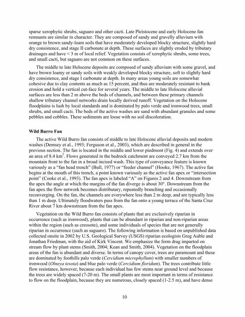
Two curious aspects of the Wild Burro fan probably result from the wash network reworking

its floodplain for thousands to tens of thousands of years. One is that the longitudinal profile of

the largest channel system on Wild Burro fan is segmented (Fig. 5) with the downstream

segment steeper than the upstream segment. The inflection point connecting the two linear

segments is located on the fan at the downstream end of a large expansion reach (location B on

Fig. 2). Many alluvial fans have fairly straight profiles or decrease in gradient in the downstream

direction forming a smooth concave-up profile. The “segmented fans” that have been discussed

previously (e.g., Bull, 1964; Denny, 1967) are in fact segmented fan-complexes where the

longitudinal profiles cross landforms of differing age. In those cases, fan-profile gradients

decrease down slope because they are on progressively younger fan surfaces as a result of the

shifting of the locus of deposition in response to climate change, tectonism, or intrinsic factors

(Cooke et al., 1993). The profile on Figure 5 does not cross landforms of differing age, however.

The fan head trench and the upper third of the fan are incised into a steeper and coarser-grained

middle Pleistocene fan remnant preserved in the upper piedmont (Fig. 4). The wash in the fan

head trench does not change gradient as it extends onto the Wild Burro fan, but down slope the

distributary network intersects the surface of the Pleistocene fan, at distance of 2,230 m on

Figure 5. Below that position the washes flow down the gradient imposed by the older fan

surface and its resistant sediments. The petrocalcic soils of the Pleistocene deposits locally crop

out in channel beds, except in the vicinity of the change in fan gradient (Fig. 5). Prior to the late

Pleistocene, the middle Pleistocene fan was truncated low on the piedmont (Fig. 4), perhaps by

the ancestral Santa Cruz River. This constituted a minor base-level fall, and may explain why the

Wild Burro fan profile diverges slightly from the Pleistocene fan profile at the downstream end

of the map (Fig. 5). In other regions with perhaps higher sediment yields or rising base levels,

younger fan deposits bury the toes of older fans. This did not happen on Wild Burro fan, at least

during the Holocene. The fan head trench and the upper part of the Wild Burro fan, where the

channels are large, are incised below the petrocalcic soil horizons of the Pleistocene fan remnant.

Lower on the fan where the channels are smaller and generally shallower, stream flows

apparently have not generated the basal shear stresses necessary to incise through the Pleistocene

petrocalcic soils.

The second interesting aspect is that the contour lines on the Wild Burro fan are crenulated

by the wash network, but are only slightly convex down slope. We suspect this reflects the fact

that the channel network on the Wild Burro fan has not aggraded or incised significantly during

the Holocene, but rather has been reworking its own floodplain sediments. Aggradational fans, in

13

contrast, have contour lines that are markedly convex in the downstream direction. The Wild

Burro fan should be considered an active, reworking type of fan.

Figure 5. Graph showing surveyed longitudinal profile of the Wild Burro fan following the main

wash along the length of the flood inundation map (Fig. 2). The bed of the main wash is depicted

with red dots and points on the Pleistocene fan remnant are depicted with closed black circles.

STORM EVENT AND FLOOD SIZE

The Wild Burro flood occurred in the evening on July 27, 1988. In early 1990 there was

obvious and extensive evidence of the recent occurrence of a large flood, including vertical

channel banks, abundant floated debris, and widespread fresh sediment. Although there were no

eyewitnesses, we were able to bracket the date of the flood to a 2-week period by talking with

people who had visited the site before and after the event (House, 1991). National Weather

Service atmospheric radar and rainfall data allowed us to pinpoint the flood date, and determine

that antecedent hydrological conditions and the storm itself were optimal for extreme flooding.

Rain had fallen in the general area on 4 of the 5 days preceding July 27, thus pre-wetting the

ground. In the afternoon of July 27, a thunderstorm developed over Wild Burro fan, and the

rainfall further reduced the normally high infiltration capacity of the sandy washes. As light rain

continued on the piedmont, intense rain occurred over the mountains where the ~10 km2 core of

the storm cell remained relatively stationary and roughly centered on the 23 km2 bedrock

catchment of Wild Burro Wash. The thunderstorm persisted for about 1.5 hours, and during

14

about 40 minutes of that period the precipitation was imaged as the two most intense classes for

atmospheric radar data collected by the National Weather Service (House, 1991). About one-half

of the catchment received intense rain. The resulting runoff flowed from the catchment, passed

through the fan head trench, and then inundated the distributary network of washes and

floodplain areas on the active alluvial fan (Fig. 2). A modest amount of flow also was delivered

to the Wild Burro fan from the adjacent, dissected piedmont, as indicated by the in-flow arrows

along the margins of the map (Fig. 2), and some flow from the adjacent Cochie Wash fan merged

with Wild Burro floodwaters in the southwest corner of the map.

The 1988 Wild Burro flood was extreme for this drainage system. The sequence of events

that led to the flood (i.e., repeated wetting immediately followed by a thunderstorm that stalled

out and rained heavily on nearly half of the bedrock catchment) is obviously rare, but does not

allow quantification of the recurrence interval of the flood. Inspection of the aerial photograph

series indicates that over the past 65 years no other flood reworked the streambeds and trimmed

channel banks to the degree that the 1988 flood did (Field, 1994; this study). This evidence is

discussed in the section titled “Changes in the Distributary Channel Network.” Regional

regressions and envelope curves of peak discharge compared to drainage basin area give an

indication of flood recurrence interval. The Wild Burro watershed area above the head of the

active fan is 23 km2 (8.9 mi

2) and our estimate of peak discharge at the fan apex is 200 to 300

m3/s (7,060 to 10,600 ft

3/s). We discuss the discharge estimates in detail, in the section titled

“Hydraulic Reconstruction and Hydraulic Geometry.” Applying that watershed area and

discharge data to regional curves indicates that the recurrence interval for the Wild Burro flood

was at least 100 years and possibly much longer. Specifically, the flood was close to a 100-year

flood according to the relationships developed by Reich et al. (1979) and by Boughton and

Renard (1984), but House (1991) has argued that these curves overestimate the magnitude of

100-year flood events. The flood had a recurrence interval of much greater than 100 years

according to the relation developed by Roeske (1978) and exceeded the magnitude of the 500-

year flood according to the curve of Malvick (1980). The Wild Burro peak discharge also plots

close to the envelope curve delineating the largest historical floods and documented paleofloods

of the lower Colorado River basin (Enzel et al., 1993; House and Baker, 2001), attesting to its

rarity.

FLOOD INUNDATION MAPPING METHODS AND LIMITATIONS

Detailed mapping of 1988 flood inundation was possible because we discovered the flood

evidence while it was still well preserved, we were able to devote a substantial effort to mapping

flood inundation, and detailed aerial photo-topographic base maps were available to use in the

field. In this section, we describe our mapping methods and consider the limitations of our

mapping results.

Flow depths were reconstructed on photo-topographic maps made in 1984 that have an aerial

photograph base with scale of 1:2,400 (not to be confused with the more common scale of

1:24,000) and contour interval of 2 ft (~60 cm). Wash sediments appear as bright, light-colored

areas compared to the less bright floodplain deposits and older soils, and dark-colored plants.

Both small and large washes are evident on the aerial photographs and in the topographic

15

contours. Individual trees and channel banks can be identified on the large-scale maps, which

allowed precise navigation and mapping in the field.

Evidence of high-water level was abundant in 1990-91, and we used four types of high-water

indicators to construct the flow-depth map (Fig. 2). Flotsam (leaves, twigs and small branches)

deposited at the margin of quiet water provided the best indication of high-water level. Slack

water deposits (silt and fine sand) indicated a minimum level of high water. Flow-swept bushes

provided a crude indication of the flow-depth category, after we determined this occurred where

the flow was deeper than 20 cm. Floating debris can be piled above the mean water surface to a

height equivalent to the kinetic energy head where relatively deep, high-velocity flow impinged

on trees, bushes or banks. The tops of debris piles (twigs, branches and whole bushes and cacti)

thus indicated the local maximum water level. We relied most on flotsam lines and slack water

deposits.

An additional criterion was used to identify the margin of flooding and the shallowest flow-

depth category on the floodplain. Where flow was shallow on the floodplain, silty sediment was

deposited, and we presume this was suspended sediment retained at the surface as flood waters

infiltrated. Scattered, fine-grained organic detritus generally was not present on this sediment.

Adjacent areas that were not flooded were sand-rich at the surface and hosted organic detritus,

and thus tended to reflect more light and to “crunch” underfoot. This evidence allowed accurate

identification of the edges of flow on the floodplain.

Abundant deposits of flotsam and slack-water sediments allowed direct measurement of

apparent water depth, the depth measured from the inferred high-water surface to the post-flood

bed or ground surface. Five categories of apparent water depth were used for the purpose of

mapping and are shown color-coded on Figure 2. Apparent water depth was measured directly,

and the depth-category boundaries were determined in the field. Field locations were identified

on the photo-topographic maps by pacing the distance from landmarks obvious both in the field

and on those maps. For practical reasons, the deepest category (red on Fig. 2) has no specified

upper boundary, but the deepest apparent water depth we observed was close to 200 cm near the

fan apex.

The flood inundation map was digitized, registered, and rectified in order to remove

distortion and to accurately place the inundation into a geographic information system (GIS)

framework. As was described above, flood inundation was mapped in the field on 1:2,400-scale

aerial photo-topographic sheets made in 1984 by Cooper Aerial Photography. Each sheet covers

one section (one square mile), with overlap onto adjacent sections. Inundation mapping involved

six sheets, identified by their section numbers within Township 11 S, Range 12 E. Flooding

covered large areas of sections 22, 28, and 29, the southern edge of section 21, and corners of

sections 27 and 32. The field sheets were spliced together by hand and map unit contacts were

traced onto one large Mylar overlay. There were no mismatches of flow-depth categories where

the field maps overlapped, but there were some minor misalignments of map unit boundaries that

were smoothed in the compilation process. The composite Mylar map was then digitized and

placed into a GIS framework. We overlaid the digital inundation map onto the 1992 digital

orthophoto quarterquads (DOQQs) available for area, and, after the locations of channels and

roads were compared between the two data sets, it was clear that there was complex internal

distortion in the inundation map. To correct this problem, we identified about 60 distinctive

points that were readily recognizable on the inundation map and on the DOQQs (road

16

intersections, channel intersections, channel bends, etc) and used them to rectify the inundation

map using a rubber sheeting algorithm in ArcGIS (ESRI, 2004). The resulting rectified

inundation map is depicted on Plate 1 (on the CD located in the map pocket of this report; GIS

data for the inundation map also are included on the CD). The areas of inundation by flow-depth

categories shown in Table 2 were calculated from the rectified map.

Table 2. Areas of inundation organized by flow-depth category and landform type, based on GIS

analysis of the rectified flood inundation map (Plate 1).

Map Unit Area, km2 percent of

mapped area*

percent of

wetted area§

Mapped area * 4.41 100.0 N.A.†

Depth 0-10 cm 0.87 19.6 38.4

Depth 10-30 cm 0.96 21.9 42.8

Depth 30-50 cm 0.25 5.7 11.2

Depth 50-100 cm 0.14 3.2 6.3

Depth >100 cm 0.03 0.6 1.2

Flooded area§

2.25 51.1 100.0

No flow 2.16 48.9 N.A. †

Channels§

0.79 17.9 35.0

Floodplain§

1.46 82.1 65.0

* Includes areas flooded and areas of no flow.

§ Includes only areas that were flooded. Total for depth categories equals 99.9 due to

rounding.

† N.A. = not applicable.

We estimated the percentage of flow in channels compared with the total inundated area

using the GIS data. The mapped flow-depth categories depicted on the inundation map do not

translate directly into flow in channels and overbank flow. Channels obviously conveyed the

deepest flow, but along some of the larger flow paths broad areas of fairly deep flow occurred on

the floodplain, and along many small channels flow was not deep. Therefore, light-colored areas

indicative of freshly reworked channel sediment along known channel systems were mapped at a

scale of 1:2,500 on the post-flood DOQQs. At this large scale it was possible to identify and map

relatively small channels fairly accurately, although there is some inherent uncertainty in

determining the boundaries between channels and adjacent floodplains. This analysis indicates

that about 1/3 of the inundation occurred in mappable channels (Table 2).

The data for downstream patterns of flow paths (Table 3) and depth-category elements

(Table 4), in contrast, were measured from transects drawn on the Mylar copy of the inundation

map. Transects were oriented perpendicular to flow and were spaced at about 500-m intervals

down the map. The rectification process mentioned above removed distortion from the

17

inundation map but did not change the general map scale. For that reason we believe that the

width data in Tables 3 and 4 are accurate.

Several caveats must be explained before interpreting the spatial distribution of flow depths

illustrated by the inundation map (Fig. 2). First, the map is not a snapshot of the flow at one

instant in time, because the flood crest took time to propagate down the wash network. Assuming

a velocity of 2 m/s for the main wash, the flood peak would have taken about 40 minutes to

propagate down the 5-km length of the map area. Flow in smaller washes and on the floodplain

would have taken longer. In addition, runoff in some small tributary washes that head on the fan

surface (see Fig. 2) was probably generated earlier in the day. Second, we infer that high-water

indicators were emplaced at the time of local peak discharge, but this may not be true. It is likely

that the water surface reached its highest altitude at the precise time of peak discharge at most

locations, but there is uncertainty in the bed level at the time of peak flow. This is of particular

concern in what we call narrow channel reaches, where the bed was scoured deeply and sediment

was redeposited. At such sites the thickness of the sediment backfill was commonly 40 percent

of the apparent water depth, as we discuss in the section titled “Bed Scour and Backfill.” The

timing of both scour and sedimentation within the flood hydrograph are not known, but we

suspect the apparent water depths on Figure 2 are underestimates of true peak flow depths

because of bed scour in narrow reaches and to a lesser degree net deposition on the floodplain.

Our use of flow-depth categories minimizes this problem. Lastly, the scale of Figure 2 is greatly

reduced from the original, thus rendering any imprecision in depth-category boundary locations

to be insignificant with one exception: washes that are in reality less than several meters wide are

shown on the map with slightly exaggerated width in order to depict the depths of flow.

(intentionally blank)

18

Table 3. Downstream patterns of widths and numbers of flow paths for 1988 Wild Burro flood.

Distance (m)* 0 516 991 1,234 1,478 1,966 2,454 2,941 3,429 3,917 4,404 4,892

Fan width (m)†

205 262 220 168 239 439 818 1,094 1,444 1,737 1,917 1,908

All observed flow paths (Fig. 2)

Number of paths4 2 3 1 3 6 15 19 32 48 56 34

Total width (m) §

144 253 176 168 173 216 567 647 631 683 718 716

Mean width (m) #

38 127 59 168 58 36 37 34 20 14 13 21

Standard

deviation64 n.a.** 64 n.a. 16 26 59 40 24 25 17 26

Minimum (m) 1 9 6 n.a. 44 6 3 1 2 2 2 2

Maximum (m) 134 244 130 n.a. 76 73 232 120 119 151 84 104

Data for flow paths excluding those generated by on-fan runoff ††

Number of paths 4 2 3 1 3 6 15 16 30 38 45 33

Total width (m) §

s.a. s.a. s.a. s.a. s.a. s.a. s.a. 640 626 657 689 714

Mean width (m) #

s.a. s.a. s.a. s.a. s.a. s.a. s.a. 40 21 17 15 22

Standard

deviations.a. s.a. s.a. s.a. s.a. s.a. s.a. 41 24 27 18 26

Minimum (m) s.a. s.a. s.a. s.a. s.a. s.a. s.a. 3 3 2 2 2

Maximum (m) s.a. s.a. s.a. s.a. s.a. s.a. s.a. 120 119 151 84 104

Note: Measurements were made along transects on the flood inundation map (Fig 2), and the transects were oriented

perpendicular to the general flow direction. Flow paths are sections (of the transects) that were flooded throughout, and are

separated from other flow paths by an intervening section of no flow. As such a flow path may be one, or may contain many,

depth-category elements. The data for depth-category elements (measured on the same transects) are in Table 4.

*Measured as the distance downstream from the top of Figure 2.

†

Measured as the distance between the outermost edges of the outermost flow paths.

§

The sum of the widths of all flow paths along a transect, and differs from fan width by the widths of intervening areas of no

flow.

#

Mean width of all flow paths along a transect with the standard deviation, maximum, and minimum of those listed below.

**n.a. = not applicable.

††

Excluded from the calculations are small washes that head on the fan and conveyed on-fan runoff. These did not convey

floodwaters generated in the Wild Burro watershed.

§§

s.a. = same as above.

19

Table 4. Downstream patterns of widths and numbers of depth-category elements, excluding on-

fan runoff channels, for 1988 Wild Burro flood.

Distance (km)* 0 516 991 1,234 1,478 1,966 2,454 2,941 3,429 3,917 4,404 4,892

All wetted elements

Sum of widths (m) 143.6 253.6 176.2 167.7 173.1 216.4 567.8 647.1 630.9 683.1 717.8 715.7

Number of elements 10 18 17 7 15 20 60 72 93 105 120 84

Depth class >50 cm

Sum of widths (m) 30.5 52.7 34.4 79.2 31.4 43.0 48.5 32.9 34.1 17.4 20.7 0

percent of wetted

width21.2 20.8 19.6 47.3 0.2 19.9 8.5 5.1 5.4 2.5 2.9 0


Mean width† (m) n.a.§ 13.2 11.5 26.4 15.7 10.7 9.7 8.2 11.4 8.7 10.4 n.a.

N.A ±6.0 ±11.9 ±19.7 n.a. ±8.0 ±6.9 ±3.1 ±5.2 n.a. n.a. n.a.

Width range (m) n.a. 18.3- 24.7- 48.8- 25.3- 22.3- 21.3- 12.2- 17.4- 12.2- 11.0- n.a.

n.a. 4.6 1.5 11.6 6.1 4.0 3.0 5.5 7.6 5.2 9.8 n.a.

Depth class 30-50 cm

Sum of widths (m) 6.7 56.4 16.2 18.3 16.8 10.7 69.2 76.5 80.2 47.9 35.7 75.9

percent of wetted

width4.7 22.2 9.2 10.9 0.1 4.9 12.2 11.8 12.7 7.0 5.0 10.6


Mean width† (m) 3.4 9.4 5.4 9.1 5.6 5.3 11.5 5.1 5.7 6.0 4.5 7.6

n.a. ±6.5 ±2.1 n.a. ±0.9 n.a. ±12.0 ±2.1 ±3.7 ±2.6 ±2.3 ±8.6

Width range (m) 4.3- 21.9- 7.0- 15.2- 6.1- 7.0- 35.1- 9.1- 16.8- 11.3- 8.5- 31.1-

2.4 4.6 3.0 3.0 4.6 3.7 2.7 1.5 1.5 3.0 2.7 3.0

Depth class 10-30 cm

Sum of widths (m) 89.9 133.8 73.2 70.1 45.7 93.6 223.1 255.7 240.5 313.3 301.4 318.5

percent of wetted

width62.6 52.8 41.5 41.8 0.2 43.2 39.3 39.5 38.1 45.9 42.0 44.5


Mean width† (m) 18.0 19.1 10.5 35.1 9.1 13.4 8.9 11.1 6.7 6.7 5.9 8.0

±18.3 ±13.9 ±4.5 n.a. ±7.1 ±7.3 ±6.9 ±12.1 ±4.5 ±8.0 ±4.1 ±7.9

Width range (m) 45.1- 41.8- 16.8- 67.1- 19.8- 24.4- 24.4- 41.8- 22.9- 54.3- 22.6- 32.0-

3.7 4.6 5.2 3.0 3.0 5.5 1.5 2.1 1.5 1.5 2.1 1.5

Depth class 0-10 cm

Sum of widths (m) 16.5 10.7 52.4 0 79.2 69.2 227.1 281.9 276.1 304.5 360.0 321.3

percent of wetted

width11.5 4.2 29.8 0 0.4 32.0 40.0 43.6 43.8 44.6 50.1 44.9


Mean width† (m) 8.2 n.a. 13.1 n.a. 15.8 9.9 9.5 9.4 6.9 6.3 6.1 9.4

±9.9 n.a. ±7.4 n.a. ±8.5 ±5.6 ±8.0 ±6.9 ±4.1 ±5.6 ±5.3 ±6.5

Width range (m) 15.2- n.a. 21.3- n.a. 30.5- 19.8- 37.5- 27.7- 18.9- 25.9- 24.4- 25.9-

1.2 n.a. 3.7 n.a. 9.8 3.7 1.5 0.6 1.5 1.5 0.9 2.4

Not wetted#

Sum of widths (m) 61.3 8.5 44.2 0 65.5 222.5 250.5 447.1 813.2 1,054 1,199 1,192


Mean width† (m) 20.4 n.a. 22.1 n.a. 32.8 44.5 17.9 24.8 26.2 22.4 21.8 36.1

±12.8 n.a. n.a. n.a. n.a. ±31.5 ±14.2 ±19.9 ±15.4 ±19.0 ±14.1 ±23.5

Width range (m) 35.1- n.a. 27.4- n.a. 62.5- 97.5- 49.7- 65.5- 71.6- 118- 72.5- 91.4-

11.6 n.a. 16.8 n.a. 3.0 15.2 2.7 1.5 2.1 1.5 3.0 3.0

Note: Measurements were made along transects on the flood inundation map oriented perpendicular to the general flow direction (Fig. 2).

Depth-category elements are sections (of the transects) that were continuously within a flow-depth category. A depth-category element may be

contiguous with elements of differing depth category or with areas of no flow. As such, a flow path (see Table 3) may be composed of one, or

may contain many, depth-category elements.

*Measured as the distance downstream from the top of Figure 2.

†Mean width of all elements in the specified flow-depth category and 1 standard deviation about that mean.

§n.a. = not applicable.

#Islands of ground not flooded within the inundation area.

20

FLOOD INUNDATION PATTERNS

Our analysis of the spatial characteristics of the Wild Burro flood is derived from Figure 2,

which depicts the spatial distribution of apparent depth of peak flow using color-coded depth

categories. The area on the piedmont encompassed by the inundation mapping is indicated on

Figure 4. Numerical data were extracted from Figure 2 and are provided in Tables 2, 3, and 4.

The general nature of the downstream branching flood waters is discussed first, followed by a

discussion of the influence that three small dirt roads had on the flow (Fig. 6) and a characteristic

channel geometry that we believe controls stream branching. Downstream patterns in various

aspects of flow are then discussed using Figures 7 and 8.

General Distribution of Flow

The area within the margins of mapped flood inundation in Figure 2 is 4.4 km2. The map

length is 4.9 km; the upper 1.1 km depicts flooding in the fan-head trench and the remaining 3.8

km of the map length spans most of the active alluvial fan. The lower 1.8 km (4 km2) of the

active fan was not mapped because of time considerations. Floodwaters inundated only 51

percent (2.25 km2) of the mapped area; thus even though the flood was extreme in magnitude

and the fan is relatively small the total area not flooded was substantial.

Flow in the distributary channels constituted about 35 percent of the inundated area, and the

remainder was flow on the floodplain. The area of small tributary channels conveying only on-

fan runoff was 1 percent of the total; thus, almost all of the mapped area of inundated ground

was from the run-on flood. Most (81 percent) of the inundated area was covered by water less

than 30 cm (~1 ft) deep (Table 2). The two shallowest flow categories (0-10 and 10-30 cm)

represent either flow in shallow sand-bedded washes or flow on the floodplain. Flow in the small

washes draining the fan surface was generally less than 10 cm deep. The three deepest flow

categories (Table 2) occurred almost entirely in sand-bedded washes, except for a few areas

where flow was 30-50 cm deep on the floodplain adjacent to large channels. The two deepest

flow categories are limited in aerial extent (7.5 percent of the flooded area) but are important

because the flood hazard is much greater in these areas of deeper, higher velocity flow. The

principal washes in the Wild Burro distributary network conveyed most of the discharge, and

thus are primarily responsible for the general distribution of flow over the fan. One large,

continuous wash system extends the full length of the fan. There are other washes, containing

deep and swift flow that extend long distances down the fan before being diminished by

branching of the flow. The flow repeatedly branched in the downstream direction, but there are

also many locations where the flow converged back together. Although much water went into

overbank floodplain areas during the flood in many locations, there were no dramatic changes in

the distributary channel network during the flood.

Comparison of the nature of flow in the fan head trench with that on the alluvial fan reveals

both differences and similarities. The boundary between these two geomorphic zones is the

location where the floodwaters spread laterally and flow became distributary. In this extreme

flood, the location where flow became distributary is essentially the same as the apex of the

active Holocene alluvial fan. The apex is located at the site labeled A on Figures 2 and 4, and at

horizontal distance 1,230 m in Figures 5, 7 and 8. Above the fan apex the flow was complex but

not distributary, because it was confined to a 300-m wide entrenched valley. Within this reach,

21

there is one main channel and typically one or more smaller channels. Water spread out in the

wash where it widens and flow went into overbank floodplain areas as shallow sheetflooding.

This flow inevitably re-collected into channels that guided the water back to the main wash. At

the apex of the fan, flow became distributary because water overtopped the north bank. If the

flood discharge had been somewhat smaller and this bank had contained the flow, however, the

floodwaters would have become distributary more than 500 m downstream from the fan apex, at

the next expansion reach downstream where the banks are low. Thus, the exact location of the

hydrologic apex (the beginning of distributary flow) is dependent on the size of the flood. On the

fan, the branching channels do not have continuous, well-defined banks in all places. Rather,

water spread out where washes widen and their banks are low or obscure, as well as where flow

overtopped defined banks. Sheetflooding inevitably re-collected into pre-existing washes, just as

it did in the entrenched reach, but the washes did not necessarily direct the flow back to a main

wash because of the breadth of the fan. This pattern of flow branching downstream, without

necessarily converging back together, distinguishes distributary flow on fans from the map

patterns typical of braided and anastomosing streams in confined valleys (Vincent, 2000).

Influence of Roads

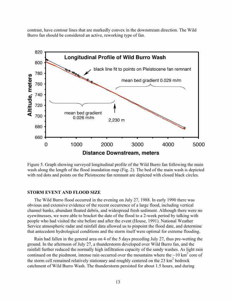
The Wild Burro fan was in a fairly pristine state in 1988, but three dirt roads influenced flow

during the flood (Fig. 6). The dirt tracks of these primitive roads are depressed slightly below the

fan surface in many places. There are no culverts where roads cross channels; rather vehicles

drive across the beds of larger channels in what are locally known as “dip sections”. The dirt

road located near the bottom of the map follows several sets of power lines, and we informally

refer to it as the power line road. It is oriented approximately perpendicular to the washes, is

maintained infrequently, and is traveled daily to weekly. This road intercepted runoff, locally

forced convergence of the flow, and in a few locations changed the direction of flow. The other

two roads are infrequently traveled dirt tracks oriented at an oblique angle to the flow paths, and

intercepted and conveyed floodwaters at many locations. The result is visible on the flood map as

discontinuous, thin, and “unnaturally” straight lines diverging 30° to 50° from the general flow

direction (Fig. 6). The fan has very low relief ( 2 m perpendicular to flow), and nearly any

alteration of the topography will influence the flow network. Therefore, even a complete

understanding of flooding on an undeveloped, active fan might not allow precise prediction of

flooding if that fan were urbanized.


22

Figure 6. Map showing dirt roads and their influence on flow during the 1988 flood. Dashed

parallel lines show the edges of roads, and the flow depth classes are as defined in Figure 2.

Solid arrows point to areas where flow was captured by the two roads that are sub parallel to

flow on the fan. Open arrows point to areas where flow was diverted by the power line road that

is approximately perpendicular to the flow direction.

Expansion/Contraction Channel Geometry

Channels on the Wild Burro fan exhibit a striking geometry marked by spatially repetitive

change in width, depth, and bed gradient. We informally refer to this as an expansion-contraction

pattern. This pattern is particularly obvious along the main wash (Fig. 2), but was evident in the

field along most washes. We also have observed this pattern along streams on other desert

piedmonts (Vincent and Smith, 1997). That there are wide reaches along desert washes has been

recognized for more than a century (McGee, 1897). Important features along other arid washes

23

include discontinuous gullies and arroyos with their prominent head cuts and associated plunge

pools (e.g., Bull, 1997). The absence of the abrupt transitions at headcuts distinguishes

expansion-contraction channels from discontinuous gullies and arroyos.

On the Wild Burro fan, the channel pattern consists of narrow reaches that are deep and have

distinct channel banks, alternating with expansion reaches that are wide and shallow and have

low or indistinct banks. Narrow reaches are conspicuous on Figure 2 at the sites labeled 13 and

1. Expansion reaches are conspicuous on Figure 2 in between the sites labeled 13 and 1 and at

the site labeled B. The longitudinal bed-profiles are concave-up in the narrow reaches and are

convex-up in the expansion reaches. Systematic variation in channel width (and associated

variations in depth and bed gradient) is repetitive over long distances, the expansion/contraction

pattern occurs over a large range in channel size, and scaling relations exist among geometric

and hydraulic parameters (Vincent, 2000). Increasing gradient and channel narrowing causes the

flow to accelerate and deepen (and scour) upon entering the narrow reaches, whereas decreasing

gradient and channel widening causes the flow to decelerate and shallow (and presumably

deposit sediment) upon entering the expansion reaches (Vincent, 1999). The geometric pattern is

likely the result of the spatial alternation of the hydraulics during high flow, from supercritical to

subcritical and back (Vincent, 2000; Vincent and Smith, 2001). There is apparently an

equilibrium of channel form and processes operating during large floods in these systems. The

expansion/contraction pattern is an integral part of the distributary network (Vincent, 2000), in

that the flow branches only at expansion reaches (Fig. 2). Usually the branches are located in the

upstream half of the expansion reaches. Flow typically does not go overbank in the narrow

reaches because these reaches are deep and prone to scour. In the aggrading expansion reaches,

however, flow diverges toward low or even nonexistent banks and thus water can pass onto the

floodplain or into distributary channels. In this way the flow branches downstream.

Downstream Patterns of Flow in the Distributary Network

In order to explore the nature and implications of the flow network we discuss patterns of

flow in the downstream direction in a successive manner, considering both the source of the

water and the apparent depth of flow. First we discuss the number of flow paths irrespective of

the source of flow using Figure 7A, and then we exclude the small channels that conveyed runoff

that was generated on the fan for the remainder of the discussion (Fig. 7B and 7C; Fig. 8; Table

4). Although these small “on-fan runoff “ channels compose only 1 percent of the wetted ground

they add significantly to the number of flow paths present on the fan, the mean width of areas of

no flow, and to a lesser degree the mean width of flow paths. Their exclusion from our analysis

allows us to focus on the “run-on” flood in the distributary network that originated in the bedrock

catchment. In addition, on-fan runoff channels are insignificant from a hazards perspective,

because flow in them was narrow (generally less than a meter or two wide) and shallow

(generally less than 10 cm deep). For those two reason we largely omit the on-fan runoff

channels from the discussion.

The result of distributary flow is a dramatic increase in the number of flow paths (Fig. 7;

Table 3) in the downstream direction. Most of the entrenched reach was flooded, with water

occupying 1 to 4 flow paths, but on the fan the number of flow paths increased downstream. If

all flow paths are considered the number increased downstream, apparently at an increasing rate,

to a maximum of 56 (Fig. 7A). If the on-fan runoff washes are excluded, however, the number of

24

flow paths increased in a more linear fashion to a maximum of 45. In either case, the pattern of

increasing numbers is reversed, curiously, near the bottom of the mapped area of the fan; this

may be partially explained by the concentration of flow into the dip sections in the power line

road (Fig. 6). The pattern of increasing numbers of flow paths roughly parallels the increasing

width of the fan and the distributary network, which is the width between the outer most

distributary flow paths (Fig. 7B). Below the apex, the fan width increased systematically, but

stopped increasing at distance of 4,500 m, where it encountered external obstacles — the

coalescing of flow from adjacent fans. The margin of flow from Wild Burro Wash is, therefore,

slightly subjective below that position.

The number of flow depth-category elements also increases in the downstream direction (Fig.

8A; Table 4). The pattern is most dramatic for the two shallowest flow-depth categories (< 10

and 10-30 cm), as the number of elements was less than 7 in the fan head trench and increased to

50 or 60 near the bottom of the map. The number of elements in the 30-50 cm depth-category

changed less dramatically, increasing downstream to a maximum of 15. The number of elements

where the flow was greater than 50 cm deep decreased from 3 or 4 (typically) in the upstream

reaches to 2 (typically) in the downstream portion of the mapped area. The primary consequence

of branching, therefore, is a dramatic increase in the number of sites of shallow flow (Fig. 8A).

The mean width of the flow paths decreased downstream, in a statistical sense, from 58 to 15

m (Fig. 7C). The range of widths for individual paths was large, however, and flow paths wider

than 70 m are found at all positions down the fan. The mean width of depth-category elements

also decreased downstream (Fig. 8B; Table 4). Curiously, the mean element width (as measured

from the transects) for all depth-categories spans a narrow range of 5 to 12 m downstream from

the fan apex (Fig. 8B). The flow was not a sheet of water with uniform thickness. Rather,

moving transverse to the flow direction, the flow depth changed substantially over distances of a

few meters to tens of meters. Thus, accurate modeling of an alluvial fan flood will require high-

resolution topography.

Although each flow-depth category is represented along the length of the map, their

contribution to the cumulative width of wetted ground changes. Flow less than 30 cm deep

(green and blue on Fig. 2) dominates the map, but the percent of wetted ground in this category

changes from 60 or 70 percent in the upstream portion of the mapped area to closer to 90 percent

near the downstream end of the map (Table 4). Conversely, flow greater than 50 cm deep (red

and orange on Fig. 2) changes from about 20 percent of the wetted ground in the upstream areas

to less then 5 percent in the downstream areas.

Statistically the flow shallowed in the downstream direction, as indicated by the increasing

dominance of the shallowest depth-categories. This also is true for the deepest observed flow.

For practical reasons, the deepest category (red on Fig. 2) has no specified upper boundary, but

the deepest apparent depth we observed and noted on the field maps was close to 200 cm near

the fan apex, whereas it was just over 100 cm at the bottom of the mapped area. These relations

indicate that deep, high velocity flow is more important from a hazards perspective in the upper

part of the fan.

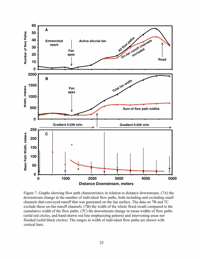
25

Figure 7. Graphs showing flow path characteristics in relation to distance downstream. (7A) the

downstream change in the number of individual flow paths, both including and excluding small

channels that conveyed runoff that was generated on the fan surface. The data on 7B and 7C

exclude these on-fan runoff channels. (7B) the width of the whole flood swath compared to the

cumulative width of the flow paths. (7C) the downstream change in mean widths of flow paths

(solid red circles, and hand-drawn red line emphasizing pattern) and intervening areas not

flooded (solid black circles). The ranges in width of individual flow paths are shown with

vertical bars.

26

Figure 8. Graphs showing depth-category element characteristics in relation to distance

downstream. (8A) the downstream change in the number of individual elements for four depth-

categories, excluding small channels that conveyed runoff that was generated on the fan surface.

(8B) the mean widths of elements in each depth-category. Two depth-categories (50-100 cm and

>100 cm) were combined for this analysis, and the colors used for depth-categories are

coordinated with those on Figure 2.

The cumulative width of wetted ground does not show a uniform increase in the downstream

direction (Fig. 7B). In contrast to the patterns mentioned above, it consists of two distinct

reaches. On the upper half of the map the sum of the widths of flow paths appears uniform,

averaging 188 m and ranging from 144 to 253 m. This 2-km long reach straddles the fan apex

with generally uniform cumulative widths of flow paths, yet the space available for flooding (the

width of the distributary network) increases from 300 m to 440 m moving down that reach.

There is an apparently abrupt increase in this parameter, to 567 m, that is roughly coincident with

the break-in-slope of the longitudinal profile (Fig. 5). Downstream of that point the width of

wetted ground increased linearly to about 700 m (Fig. 7B). This evidence suggests that the width

of wetted ground was controlled by the input discharge, the fan gradient, and to a lesser degree

the scaling relation between discharge and flow width. The number of flow paths and the mean

width of flow paths were not obviously influenced by fan gradient, and thus were apparently

controlled by discharge and distance down the fan (a proxy for branching frequency).

27

The area of ground not flooded within the distributary network increased downstream,

because the total width of the fan increased downstream much more than the width of wetted

ground (Fig. 7B). The area of ground not flooded was small upstream from the fan apex, but

increased to about 60 percent of the fan width at the downstream end of the mapped area. The

width of individual areas of no flow, however, was small everywhere on the fan. The mean width

of areas of no flow was generally less than 30 m irrespective of position on the fan (Table 4).

Downstream from the fan apex, the widest individual areas of no flow ranged from 50 to 120 m

wide, and the downstream increase in that parameter is slight (Table 4). Again, the small

channels draining the fan surface are excluded from the calculations above because they are

insignificant from a flood hazards standpoint. The implication for flood hazard concerns is that

the areas of no-flow are relatively small and their sizes may be independent of position on the

fan.

In conclusion, the primary consequence of flow branching downstream was a dramatic

increase in the number of sites of shallow flow and the increasing dominance of the cumulative

width of shallow flow. Channels conveying deep and swift flow, however, occurred at all

distances down the fan, and areas of no flow were narrow irrespective of position on the fan.

Hydrology of the Distributary Network

The source-area hydrology for distributary networks is more complicated then for tributary

networks in the following way. There are four distinct drainage networks (runoff sources)

associated with alluvial fans (Cooke et al., 1993), and all are illustrated by the Wild Burro

example (Figs. 2 and 4). The bedrock catchment contains a tributary network that conveys to the

piedmont flows that vary greatly in magnitude. Such flows are then conveyed by the distributary

network of washes on the active alluvial fan (Fig. 2). In the upper piedmont area, composed of

old eroded fans in this example (Fig. 4), tributary wash networks convey runoff from the fan

remnants to the margins of the distributary network on the active fan. Within the active fan, local

tributary networks of small channels convey runoff generated on the fan surface into the

distributary network of larger washes (Fig. 2). There is an additional complication in that the

distributary networks of adjacent fans may coalesce at some position on the piedmont. The

distributary network on the Wild Burro fan received flow from the Cochie Wash network to the

northwest (see Fig. 2). Thus any one distributary-wash on an active alluvial fan will receive flow

from two sources (the bedrock catchment, and localized “on-fan runoff” areas), and may receive

flow from two other areas (the adjacent dissected portions of the piedmont, and from adjacent

active fans). This means that streamflow statistics (such as magnitude/frequency relations) may

not be uniform over the fan area, and may not even vary spatially in some systematic way. The

use of bedrock catchment area as a proxy for discharge may still be valid for a fan apex, but is an

oversimplification for channels within the distributary network.

The pattern of a distributary network is not like the roots of a tree or an inverted tributary

network. Tributary networks converge in the downstream direction, with rare exceptions, and

typically channels steadily increase in size downstream. Distributary networks branch in the

downstream direction, but locally branches also converge (Figs. 2, 6, and 9). Thus distributary

washes decrease in size in the downstream direction in general, but also may increase in size

locally. For this reason it is not obvious how a meaningful stream-order system (e.g., Horton,

1945) for links or branches of distributary networks would be constructed. Lastly, although the

28

mathematical properties of “trees” (Peckham, 1995) could appropriately be applied to the

hydraulic geometry of tributary networks they cannot be meaningfully applied to distributary

networks.

Inundation of Landforms of Differing Age

In order to evaluate the usefulness of surficial geologic mapping in delineating piedmont

flood hazards, we compared the flood inundation map (Fig. 2) to the surficial geologic map (Fig.

4) in a GIS framework. The surficial geologic map depicted on Figure 4 was developed primarily

using 1:12,000- and 1:24,000-scale aerial photographs from 1979 and 1983. Thus, the geologic

map unit boundaries are not based on the 1988 flood inundation or the relatively minor changes

in the landscape that resulted from that flood. Inundation during the 1988 flood occurred almost

entirely on middle and late Holocene deposits, including active channels and young overbank

areas with minimal soil development. Approximately 98 percent of the Wild Burro flood

inundation occurred on those surfaces. Minor inundation of older Pleistocene surfaces occurred

in a few places along the northern margin of the flood, and very locally along the eastern margin

of the fan. The primary reason for the lack of inundation of older alluvial surfaces is that they are

substantially elevated (one to several meters) above adjacent Holocene surfaces. This illustrates

that geomorphic mapping combined with consideration of local topographic relief can provide a

reliable and conservative prediction of flood-prone areas on desert piedmonts.

SEDIMENT EROSION AND DEPOSITION

Three types of channel change can occur during floods: new channel formation, bank

erosion, and bed scour and (or) filling. The Wild Burro flood, however, passed through

preexisting channels that were uniquely suited to convey the flow. As discussed herein, only bed

scour and backfilling were substantial during the flood.

Changes in the Distributary Channel Network

No major channels were formed and no other substantial changes occurred in the distributary

channel network of Wild Burro Wash during the 1988 flood. The fact that we were able to

navigate the fan and map inundation patterns using pre-flood aerial photo-topographic maps

attests to the lack of change in channel patterns during the flood. Examination of before and after

aerial photographs of the whole fan indicates that many small channels in the system became

more obvious as a result of deposition of fresh channel sediment and minor channel widening,

but the fundamental character of the network was the very similar before and after the flood (Fig.

9). Even in the major channel expansions downstream from the fan apex, where broad sheets of

freshly deposited sand and fine gravel were evident after the flood, changes in the total extent of

fresh sand were minor (sites X and Y on Fig. 9). The channel network was more continuous in

appearance after the 1988 flood; this is most likely due to removal of vegetation from some

channel areas and deposition of fresh channel sediment in other areas.

29

Figure 9. Aerial photographs showing Wild Burro alluvial fan before and after the July 27,1988

flood. The black dashed lines on both photographs show the network of major channels as it was

in 1979. The channel network was more continuous in 1992 after the flood and many small

channels are more evident, but the basic outlines of the system changed very little even in the

major expansion reaches labeled X and Y. The northern distributary channel network (N) was

linked more directly to the main channel after the flood. Aerial photograph from 1979 was

provided by the Pima County Flood Control District. Aerial photograph from 1992 was compiled

from USGS digital orthophoto quarterquads of the Marana and Ruelas Canyon 7.5’ quadrangles.

30

The lack of substantial channel changes during the 1988 flood is in marked contrast to the

behavior of several other water-flood dominated alluvial fans in southern and central Arizona

that have experienced extreme floods (Field, 1994; 2001; Pearthree et al., 2004). The Wild Burro

distributary channel network may be intrinsically more stable than the other fans because of

greater vegetation density or more cohesive bank material. It also is possible that dramatic

channel changes occur in some floods because conditions are ripe for their occurrence as a result

of more gradual changes that occurred during previous events. Field (1994) suggested that local

streambed aggradation during smaller flow events could set the stage for avulsion during

subsequent floods. Large floods, such as the 1988 flood, may cause minor changes in the system

that facilitate more substantial changes in the next large flood. An example of this latter

phenomenon may exist on Wild Burro fan. The relatively modest channel system along the

northern margin of the fan (site N on Fig. 9) is now more directly linked to the main channel

system by several small channels visible as white lines on Figure 9. Future large floods may

exploit and enlarge these channels, diverting increased amounts of flow. If that occurs, it will

likely result in a major change in the distribution of water and sediment on the active fan. For

example, Vincent (2000) used a channel network simulation to show that among the most

important controls on network geometry is the presence or absence of branching channels close

to the fan apex, and the proportion of the flow diverted into branches. Areas where multiple

channels diverge at major channel expansions (such as site X on Fig. 9) also are potential

locations of channel change because one branch may become dominant. Relatively modest

changes in loci of deposition in the expansion reach or channel incision at the downstream

margin of the expansion could alter the distribution of flow between the distributary channels.

Although inundation was very extensive in the area near site X during the 1988 flood, the

greatest amount of flow went down the left (viewed looking downstream) channel below this

expansion. (Site X on Fig. 9 is labeled B on Fig. 2.) Given the greater size of the left channel and

the fact that its gradient is steeper than the central and right channels, this situation is probably

fairly stable in the short term, but over a period of centuries to millennia the distribution of

sediment and flood flows likely will change substantially in this area.

Bank Erosion

Bank erosion was ubiquitous, but nowhere was it dramatic. We observed that almost all

banks had been trimmed and left standing vertical. Bank erosion can occur through tractive

forces during the floods, and by bank collapse after floods. The shape of the banks and the nature

of their contacts with bed material were consistent with channel widening by bank erosion during

the flood. This includes the near vertical extension of the bank into the subsurface against which

rests 1988 backfill sediment (Fig. 10). That type of observation was made in trenches excavated

into the bed of narrow channels, which are discussed in the next section. Bank collapse after

floods results from failure of saturated bank material (Leopold and Miller, 1956), is common in

arroyos with very high banks, and is indicated by the presence of blocky or rumpled bank

material resting upon bed sediment. That type of evidence was observed only locally, and only

where the banks were high ( 1 m). The magnitude of bank erosion was relatively moderate, as

indicated by two types of evidence. Although we did not systematically study bank erosion

patterns, we observed bank features, such as the length of exhumed tree roots, and thereby

gained the impression that lateral erosion of banks was commonly less than a meter. At only one

location did field evidence indicate that lateral erosion of banks was large (12 m), but this

31

erosion added only 20 percent to the width of the wash at that location, which was an expansion

reach. The second type of evidence comes from the logs of trenches (discussed in a the next

section) excavated across narrow reaches. In all the trenches lateral erosion was less then 1 m,

and in many cases was too small to be quantified. For six trench logs where channel widening

could be quantified the average widening was 7 percent (range was 5 to 11 percent).

Bed Scour and Backfill

During the flood, the bed was scoured deeply and sediment was subsequently deposited at

the same location, in narrow reaches. Although bed scour is often ignored during flow

reconstruction studies, it can be an important factor because of the influence of cross-sectional

area and hydraulic radius on hydraulic calculations. We attempted to reconstruct the hydraulics

at 20 narrow reaches, as discussed in the following section, and were concerned about the

influence of bed scour. (Sites are labeled with numbers on Fig. 2.) In this report the deepest level

(lowest altitude) of scour during the 1988 flood is called the scour limit, and the overlying

deposits are called backfill. At each hydraulic reconstruction site, two to four trenches were

excavated in the spring of 1991 across the channel (perpendicular to the flow direction). There

were no substantial flow events between 1988 and the trench excavations. The scour limit was

deciphered (Table 5) using four criteria: discolored sediment, the shape of the erosional contact

at trimmed banks, micro-stratigraphy, and the presence of old roots.

Sediment color was used to differentiate young flood deposits from older sediments.

Recently transported granitic sand in active waterways is always light colored, or “white”. Left

undisturbed, however, sediments undergo discoloration (by various soil forming processes) that

progresses with time. In this setting soils change color through time following this generalized-

color sequence: from “white” to “yellow” to “brown” to “orange” to “red”. In channel-bed

excavations the presence of discolored sediment is important because it indicates in-place soil

formation over at least centuries of time, as opposed to deposition by a historical flood. Using the

channel cross-section of Figure 10 as an example, none of the discolored sediment, and more

specifically the “yellow” sediment, could have been deposited by the 1988 flood.

The nature of contacts at the channel bank was critical for deciphering the scour limit, where

more than one package of fresh-looking sediment was observed overlying obviously discolored

sediment. Notice there are two beds of fresh looking sediment on Figure 10, and we determined

that only the upper bed was deposited in 1988 using the following evidence. The base of

virtually every channel bank was trimmed by the flood and left standing nearly vertical. Trench

excavations inevitably revealed a vertical contact extending down from a trimmed bank into the

channel bed. The vertical contact turned sharply at depth, often creating a sub-horizontal step in

older bank material. A nearly right angle corner in the erosional contact is visible on both banks

in the example of Figure 10, although on one bank the step cut into discolored sediment is

narrow. The erosional contact extended sub-horizontally under the channel as a traceable

stratigraphic horizon (Fig. 10). The vertical contact, erosional corner of the contact, and

contiguous sub-horizontal stratigraphic horizon were interpreted as the scour limit of the most

recent large flood, in this case the 1988 flood. Because the bed sediments contained multiple

stratigraphic horizons, we tended to study the relations at both banks and then trace the scour

limit toward the channel center.

32

Figure 10. Graph showing example of a channel cross-section used in hydraulic modeling of

peak flow in narrow reaches for the 1988 flood, including the scour limit and backfill sediment.

The colors used are generalizations of the sediment colors as they appeared in the field. Bed

sediment deposited by the 1988 flood was identified based on the fresh, unoxidized character of

sediment that also did not contain sizable roots, and was underlain by an erosional contact (the

maximum depth of scour) which had abrupt corners at the channel banks.

Plant roots also can indicate deposit age (Fig. 10). Recently transported channel-bed

sediments in the study area contain small-scale or micro-scale stratigraphy, dominated by

multiple fining-upward sequences that are each several centimeters to a decimeter in thickness,

and commonly have intervening black-sand layers. It was not necessarily obvious, however,

whether multiple sedimentary sequences were the result of multiple pulses of sedimentation

during one flood or were the result of multiple floods. The observation within beds of plant roots

too large to have grown since the 1988 flood indicated that the sediment packages containing the

roots were not deposited by the 1988 flood. Roots found on a stratigraphic contact were not used,

because roots exhumed from banks by the 1988 flood were observed still attached to the banks.

Thus, old roots could end up near the base of a younger flood deposit.

Three conclusions can be drawn from the work deciphering channel bed scour-limits. First,

the flood scour-limit can indeed be deciphered by careful examination using the stratigraphic

criteria discussed above. Second, sandy washes of southern Arizona have remarkably flat beds,

but the bed scour-limits observed were almost never as flat as the post-flood bed surface and

were often wavy or occasionally trough shaped in cross section (Fig. 10). This is similar to the

observations made by Foley (1978) in his study of a hydraulically steep sand-bedded stream, and

33

observations made by Leopold et al. (1966). The backfill deposits do not taper to zero thickness

at the banks, however. Instead, the backfill thickness near the banks was close to the magnitude

of the backfill thickness averaged over the cross section. Thus, excepting for occasional and

localized sites of unusually deep scour, the beds of backfill sediment were approximately tabular

in cross section. Third, as illustrated on Figure 11, the mean thickness of backfill sediment

(averaged over the cross-section) was 41 percent of the apparent depth of flow (peak water

surface to post-flood bed). It was as thin as 15 percent and as thick as 60 percent of that depth.

This relation should provide useful guidance for installation of scour-chains or other

investigations of bed scour, and serves as a cautionary reminder to those reconstructing flow in

similar settings of the uncertainty in cross sectional area.

Tc = 0.41 Ha; R2 = 0.84

0.0

0.1

0.2

0.3

0.4

0.5

0.6

0.7

0.0 0.2 0.4 0.6 0.8 1.0 1.2 1.4

Apparent Flow Depth , meters

Bac

kfill

Th

ickn

ess,

met

ers

Figure 11. Graph showing relation of apparent flow depth (Ha) and streambed sediment backfill

thickness (Tc). Data for select narrow reach sites located on Figure 2 (also see Table 5). Both

variables are cross section averages.

Net aggradation, or net lowering, of the ground surface caused by the flood is difficult to

evaluate, but as far as we could tell such changes were small. The pre-flood base maps that we

used included contour lines with interval of about 60 cm (2 feet). Using that criterion, we did not

detect major changes in bank height. Scour and backfill data are not available for expansion

reaches, although these reaches probably were sites of net sediment deposition. Deposition of

sediment in overbank areas was widespread but thin, perhaps a few centimeters on average.

34

Table 5. Thickness of streambed backfill sediment in select narrow channels. [The abbreviation

“n.a.” indicates that that the data are not available.]

Reach

number

(located

on Fig. 2)

Cross-section

number

(increase

downstream)

Apparent

flow depth

Deposit

cross-section

area

Deposit

top width

Mean backfill

thickness

(cross-section

average)

Mean

backfill

thickness

for reach

m m2

m m m

1 1.90 17.28 32.00 0.54

3 1.70 9.70 22.40 0.431

5 1.40 12.99 27.60 0.47

0.48

1 0.70 0.84 4.80 0.172

4 0.45 0.86 5.10 0.170.17

2 0.20 0.14 2.10 0.073

3 0.20 0.15 2.10 0.070.07

1 0.64 1.83 7.90 0.234

5 0.53 1.10 7.10 0.150.19

1 n.a. 0.64 4.80 0.13

3 n.a. 1.01 5.60 0.185

4 n.a. 0.85 5.15 0.17

0.16

1 0.44 0.30 2.45 0.12

2 0.47 0.37 3.20 0.12

3 0.47 0.24 2.60 0.096

4 0.37 0.28 3.30 0.08

0.10

1 1.16 3.15 11.70 0.27

3 1.08 2.40 9.60 0.257

5 0.93 1.70 9.80 0.17

0.23

1 0.90 3.79 9.50 0.40

3 1.05 5.29 13.60 0.398

5 1.10 0.93 7.30 0.13

0.31

1 0.40 0.35 3.01 0.12

2 0.35 0.36 3.00 0.129

3 0.35 0.43 3.82 0.11

0.12

1 0.39 0.06 1.55 0.04

2 0.41 0.06 0.80 0.07

3 0.38 0.08 0.95 0.0810

4 0.36 0.09 1.00 0.09

0.07

1 0.31 0.21 2.50 0.08

3 0.33 0.30 3.20 0.0911

4 0.28 0.35 3.20 0.11

0.10

1 0.62 1.25 8.10 0.1512

4 0.45 1.25 7.50 0.170.16

1 1.30 18.78 34.20 0.55

3 1.30 16.06 26.90 0.6013

5 1.50 14.20 27.30 0.52

0.56

continued

35

Table 5 (continued). Thickness of streambed backfill sediment in select narrow channels. [The

abbreviation “n.a.” indicates that that the data are not available.]

Reach

number

(located

on Fig. 2)

Cross-section

number

(increase

downstream)

Apparent

flow depth

Deposit

cross-section

area

Deposit

top width

Mean backfill

thickness

(cross-section

average)

Mean

backfill

thickness

for reach

m m2

m m m

2 0.95 2.27 8.50 0.27

3 0.91 1.98 8.70 0.2314

4 0.83 2.24 8.30 0.27

0.25

1 0.51 1.52 9.20 0.16

2 0.46 1.56 8.35 0.1915

3 0.52 1.62 7.90 0.20

0.19

1 0.60 0.66 3.80 0.17

2 0.63 0.66 4.45 0.15

3 0.60 0.64 4.55 0.1416

4 0.57 0.51 4.20 0.12

0.15

1 1.30 1.00 4.40 0.23

3 1.30 1.13 4.60 0.2517

5 1.15 1.03 5.10 0.20

0.23

1 0.22 0.13 2.10 0.06

2 0.21 0.09 2.15 0.04

3 0.23 0.06 1.70 0.0418

4 0.20 0.06 1.25 0.05

0.05

1 n.a. 0.02 0.65 0.03

2 0.07 0.02 0.62 0.02

3 0.09 0.02 0.80 0.0319

4 n.a. 0.03 0.90 0.04

0.03

1 0.13 0.05 1.15 0.0420

2 0.13 0.02 0.95 0.030.03

Lastly, we observed no evidence of bank healing processes, such as laterally accreting point

bars. That most stream banks were trimmed by the flood, including opposing banks, illustrates

the lack of point bars. In addition, there are no levees or sedimentary beds laminated onto banks,

which are characteristic of silt-dominated ephemeral streams (Vincent, USGS, unpublished data,

2004). The backfill sediments were sub-horizontally stratified, and the post-flood streambeds

were remarkably planar, which is typical of sand dominated ephemeral streams (Reid and

Frostick, 1989). This evidence suggests that sedimentation on this fan is principally by vertical

accretion.

In conclusion, the Wild Burro flood passed through preexisting channels that were uniquely

suited to convey the flow, and the flood acted to construct and maintain the geometry of both the

channels and the network as a whole. Previous workers have made similar observations for near

bankfull flows in other types of streams, and used that as evidence of equilibrium of form and

process (Langbein and Leopold, 1964).

36

HYDRAULIC RECONSTRUCTION AND HYDRAULIC GEOMETRY

In order to understand the nature of local flow conditions during the flood, flow hydraulics

were reconstructed at 18 narrow reaches using data collected in 1991. The sites are located on

Figure 2 using their reach numbers. All of the narrow reaches are straight, relatively deep, and

had abundant and reliable high-water evidence preserved on both banks. The sizes of the

channels varied greatly, however, so these sites represent the full size-spectrum of washes on

Wild Burro fan. Wide expansion reaches were not modeled, because the flow was multi-

dimensional and high-water marks were less reliable.

Hydraulic Reconstruction Methods and Uncertainties

The process of reconstructing flow hydraulics involved identification of high water

indicators, evaluation of bed scour through trenching across the channel, surveying channel

cross-sectional form and high water indicators, and hydraulic modeling of flow. The primary

high water indicators identified were fine-grained slack-water deposits and lines of flotsam

composed of organic material such as twigs and leaves. Piles of larger organic debris trapped

against trees were also identified, but debris piles likely overestimate the static water level

because they were emplaced where the momentum of the flow caused the water (and floating

debris) to run-up to a super-elevated position on an immobile object. The deepest limit of bed

scour was assessed by interpreting deposits exposed in trenches excavated across the channels

(see Fig. 10 for example), as discussed in the preceding section. A longitudinal profile (Fig. 12)

and multiple channel cross-sections were surveyed for each study reach. Survey data included

the spatial position of high-water indicators; and the topography of the over-bank ground surface,

banks, post-flood channel bed, and the deepest limit of scour interpreted to have occurred in the

1988 flood.

Channel hydraulics were reconstructed using two modeling routines, both based on

Manning’s equation. For the 5 smallest channels, the slope-area method was used (Dalrymple

and Benson, 1967). The 13 larger channels were modeled with the HEC-2 step-backwater

program (Hydrologic Engineering Center, 1985). Channel geometry and the height of high-water

indicators were entered into a computer, a roughness coefficient assumed, and a trial discharge

selected. Discharge was then iterated until the water-surface profile predicted by the model

matched the high-water indicators; examples of the results are illustrated on Figure 12. Both

models embody the assumptions that the flow was steady, gradually varied, and one-

dimensional, and that the viscosity was that of clear water.

A Manning's roughness coefficient value of 0.035 was used to model the hydraulics at all

reaches. This is one of two major sources of uncertainty, and the major concern herein is that our

roughness value may be too low (smooth) because our estimated flow velocities are swift and

Froude numbers are large. Selecting a roughness coefficient for flow at ungaged sites is always

problematic. A common approach is to adopt a roughness coefficient determined from direct

measurements made at a similar site. Direct measurements (of mean flow velocity, hydraulic

radius, and water-surface gradient) allow roughness to be “back calculated” from Manning’s

equation, and this information is usually compiled as either a regime equation (e.g., Limerinos,

1970; Jarrett, 1984) or as a book of photographed reaches (e.g., Barnes, 1967). Unfortunately, no

comprehensive study of roughness coefficients based on direct measurements has been published

for waterways similar to the sandy ephemeral washes at Wild Burro. An alternative approach is

37

to use theory-based equations and account for each type of feature that contributes to flow

resistance. Grain roughness depends on the height that bed sediment particles project into the

flow (e.g., Wiberg and Smith, 1991). Given the flow depths of our study reaches, the projection

heights of sand grains and thus grain roughness was small. Channel bank micro-topography and

plant stems can impart considerable flow resistance that can be accounted for (Smith, 2004;

Kean and Smith, 2004). Form drag imparted by plants stems could be accounted for if the

objective were to model flow on the floodplain. Our study channels, however, are largely

unvegetated and are quite wide compared to the flow depths. This is a situation where bank

roughness is often ignored (e.g., Henderson, 1966). We suspect that the flow resistance in our

study reaches was dominated by form drag resulting from bedforms. We were not able to use

theoretical approaches to quantify flow resistance, because we do not know the geometry of

bedforms in the channel at the time of peak flow. For this reason, we adopted the traditional

empirical approach of using Manning’s equation.

Table 6. Measurements and observations of flow-roughness values, flow velocity, and Froude

number for flow in desert streams with fine-grained beds.

Observer /

author

Dates* ,

†Location, Stream

§Gradient

m/m

Manning’s

Roughness

Velocity

m/sec.

Froude

number

Nordin 1961, 1963 C NM, Rio Puerco0.014 –

0.016

Nordin 1962, 1963 C NM, Rio Grande0.015–

0.030

Rahn 1963, 1967 C AZ, “San Tan” 1.9 1.09 #, >1

** ††

Rahn 1963, 1967 W AZ, “Joshua Tree” 1.8 2.11 #, >1

††

Reid and Frostick 1979, 1987 Kenya, Il Kimere 0.007 >1 **

Tom Kane, USGS 1993, 1993 S NV, Cain Springs 0.025 0.018 3 1.9 #, >1

**

The authors , 1993 S AZ, Santa Cruz 0.005 >1 ** ††

Rod Roeske, USGS , 1993 S AZ, Santa Cruz 0.005 8.5

Phillips & Ingersoll 1964, 1998 S AZ, Santa Cruz 0.004 0.020 3.8 0.87 #, >1

**

Phillips & Ingersoll 1993, 1998 C AZ, Hassayampa 0.006 0.026 3.6 1.13 #, >1

**

* Date of field observation or flow measurement.

† Date of published paper, or personal communication with Kane and with Roeske.

§ Location abbreviations include S (southern), W (western), C (central), AZ (Arizona), NV (Nevada),

and NM (New Mexico).# Froude number calculated from direct flow measurements.

** Upper flow regime: standing waves built and broke over antidunes.

†† Upper flow regime: disturbance waves did not propagate upstream.

38

Figure 12. Graphs showing examples of longitudinal profiles used to model 1988 flow hydraulics

in narrow reaches. Minimum and maximum discharge estimates were obtained using the post-

flood and maximum scour depth channel cross-section geometries, respectively.

39

Our selection of Manning’s roughness of 0.035 was based on personal communications

(1991) with Ken Renard (Agricultural Research Service) and Win Hjalmarson (US Geological

Survey) who together have more than 50 years of experience as hydrologists in southern

Arizona. A value of 0.035 is not particularly low for streams in general, and several direct

measurements have yielded Manning’s coefficients substantially less than 0.035 for ephemeral

streams (Table 6). The most extensive data set is from the Phillips and Ingersoll (1998) study of

10 streams in a relatively natural state in the Sonoran Desert of Arizona for which hydraulic

measurements were made at high flow. The Manning’s roughness coefficients for those sites

averaged 0.032, and at two sand-bedded sites the roughness coefficients were 0.020 and 0.026

(Table 6). We acknowledge the uncertainty involved with our assumed roughness value, but

have found no justification for using a substantially larger (rougher) value.

The second major source of uncertainty in our hydraulic modeling of flow in narrow reaches

has to do with the relative position of the water surface and the bed at peak discharge. It is not

certain whether the high water indicators were emplaced at the time the bed had reached the

deepest level of scour. For this reason we attempted to constrain the hydraulics at peak flow by

running the model using two cross-sectional geometries. In both scenarios the high water

indicators were used to constrain the water-surface level. In one scenario we used the surveyed

post-flood channel bed as the bottom of the cross section, and this produced what is probably an

underestimate of flow area and depth because the magnitude of scour and backfill during the

flood was substantial (Figs. 10 and 11). In the second scenario we used the surveyed scour-limit

as the bottom of the cross section, and this produced what is probably an overestimate of flow

area and depth. We believe a cross-sectional area bounded by the scour-limit is a maximum for

three reasons. First, bed scour may not have been at its deepest level at the time the flood crested.

Second, the scour-limit may be deeper than the mean bed-level for the flow if the scour-limit

represents an asynchronous surface that formed at the troughs of migrating bed forms (Foley,

1978). Lastly, the high-water indicators might have been slightly superelevated if they were

emplaced by translatory waves or surges resulting from the collapse of standing waves (Bean,

1977; Hjalmarson and Phillips, 1997; Phillips and Ingersoll, 1998). Because we used two bed

position scenarios, we present our hydraulics results as pairs of values for each reach (Figs. 12,

13, and 14; Table 7).


40

Table 7. Selected hydraulic parameters derived from modeling peak flow for the 1988 flood

through narrow reaches of all sizes on Wild Burro fan. [Parameter letters with subscript (sc)

denote modeling results assuming that peak flow occurred at the time of maximum scour.

Parameter letters without subscript denote modeling results assuming that the base of the cross

section was the post-flood channel bed at the time of peak flow.]

Reach

No.

Peak

Discharge

(m3/s)

Froude

No.

Top

Width

(m)

Area (m2) Maximum

depth (m)

Avg.

Velocity

(m/s)

Width/Depth

ratio

Q Qsc F Fsc W A Asc D Dsc V Vsc W/D W/Dsc

1 200 300 1.24 1.32 40 47.9 58.9 1.5 2.3 4.2 5.2 27 17

2 15 20 1.30 1.38 15 5.9 6.8 0.6 0.8 2.5 2.9 25 19

3 1.1 1.3 1.17 1.15 7.3 0.8 1.0 0.2 0.3 1.3 1.4 36 24

4 15 20 1.18 1.15 12 6.2 7.1 0.7 0.9 2.5 2.8 17 13

6 4 5 1.22 1.16 5.4 1.8 2.1 0.5 0.6 2.2 2.3 11 9

7 75 100 1.35 1.38 26 19.6 24.0 1.2 1.6 4.2 4.2 22 16

8 40 80 1.31 1.54 18 11.9 16.6 1.0 1.7 3.4 4.8 18 11

9 2 3 1.04 1.12 4.9 1.2 1.5 0.3 0.4 1.6 2.0 16 12

10 1 1.2 1.15 1.12 2.6 0.6 0.7 0.4 0.5 1.8 1.9 6 5

11 2 3 1.14 1.22 6 1.2 1.6 0.3 0.5 1.6 1.9 20 12

13 175 300 1.37 1.49 40 40.8 52.7 1.3 2.5 4.4 5.7 31 16

14 35 40 1.22 1.25 16 11.1 11.4 1.0 1.2 3.2 3.5 16 13

15 10 15 1.19 1.2 12 4.4 5.6 0.5 0.7 2.3 2.7 24 17

16 10 15 1.25 1.29 10 3.8 4.9 0.6 0.9 2.6 3.0 17 11

17 40 50 1.40 1.48 18.5 11.7 12.9 1.2 1.5 3.4 3.9 15 12

18 0.5 0.6 0.91 0.88 3.3 0.5 0.5 0.2 0.3 1.1 1.1 16 11

19 0.04 0.06 1.02 1.13 1.4 0.06 0.07 0.08 0.1 0.6 0.8 18 14

20 0.08 0.12 0.92 0.93 1.5 0.11 0.14 0.09 0.13 0.8 0.9 17 12

41

Hydraulic Modeling Results

The hydraulic modeling results for the Wild Burro flood (Table 7) indicate that flow

velocities in narrow channel reaches were rapid, typically 2 to 3 m/s but as high as 4 to 5.7 m/s.

The peak discharge at the fan apex (reach 1 in Table 7) was between 200 and 300 m3/s, which is

also high given the relatively small area of the catchment (Enzel et al., 1993; House and Baker,

2001). The hydraulic modeling also suggests that Froude numbers (F) were high at peak

discharge, irrespective of which cross-sectional geometry scenario was used. This indicates the

flow was either close to critical (F=1) or was supercritical (F>1) in narrow reaches, which had

bed gradients between 2 and 3 percent. Reach-averaged Froude numbers ranged between F=0.88

and F=1.54, and for all but two reaches were greater than 1. Some readers experienced with

perennial streams may be surprised by these high Froude numbers, because supercritical flow is

rare in perennial streams (e.g., Jarrett, 1984) and where it does occur is thought to persist only

over very short stream reaches (e.g., Trieste, 1992). For that reason we now place our results into

context.

The Froude number is defined as the inertial force divided by the gravitational force of a

flow, and is important because it quantifies alternate states of flow: subcritical and supercritical

(e.g., Henderson, 1966). Subcritical flow also is known as “tranquil” flow or the lower flow

regime, and supercritical flow is also known as “shooting” flow or the upper flow regime. A

hydraulic jump occurs at the position of the transition between supercritical and subcritical flow.

The Froude number is calculated from measurements as flow velocity divided by the square root

of the product of flow depth and the acceleration of gravity. As shown on Table 6, critical and

supercritical flow have been identified in many sand-bedded ephemeral streams at flood stage. In

that context, the results of our hydraulic modeling are within reason. In addition, our high Froude

numbers are consistent with the thoughts and observations of Bean (1977), Foley (1978), French

(1987), Blair and McPherson (1994b), and Grant (1997).

Downstream hydraulic geometry relations are evident in the discharge, width, depth, and

velocity data for the Wild Burro flood (Figs. 13A and 14), just as they are for other streams

(Leopold and Maddock, 1953). Hydraulic geometry relations have been demonstrated for other

types of streams in arid lands such as those within arroyos (Leopold and Miller, 1956) and of

course for meandering streams in humid lands (Wolman, 1955), as illustrated for Brandywine

Creek on Figure 13B. The exponent of width/discharge scaling relations is typically 0.5 (Leopold

et al., 1964), whereas it is 0.4 for Wild Burro narrow reaches. This lower value is not

unprecedented, however, as the data for Brandywine Creek illustrate (Fig. 13B). The exponents

for the depth and velocity relations (Fig. 14) also are within the range of previous observations

(Leopold et al., 1964, p. 244).

There are two differences, however, between downstream hydraulic geometry relations for

ephemeral expansion/contraction streams and those for other streams. One is that the

downstream direction is reversed, in that downstream is to the right on Figure 13B for tributary

networks whereas it is to the left for distributary networks. The second distinction involves the

magnitude of systematic variation in channel dimensions along shorter distances. Meandering

streams, for example, exhibit relatively small but significant geometric variations through their

pool and riffle sequences (Richards, 1976). Along the East Fork River, Wyoming, for example,

riffles are about 30 percent wider than nearby pools (Andrews, 1979). Nevertheless, well-

constrained hydraulic geometry relations result even if the sample reaches were selected without

42

regard to their positions in the pool and riffle sequence. The same cannot be said for waterways

that exhibit the expansion/contraction pattern discussed here. Well-constrained downstream

hydraulic geometry relations are evident for the narrow-channel reaches on the Wild Burro fan,

as illustrated on Figures 13 and 14. Like pools, narrow reaches are an end-member of a pattern.

Unlike pool/riffle sequences, expansion/contraction sequences have large variation in width. On

the Wild Burro fan, expansion reaches are 3 to 5 times wider than the narrow reaches that supply

them. The hydraulics for individual expansion reaches was not modeled, as mentioned above, but

the data for expansion reaches on Figure 13A were estimated as follows. The flood-inundation

map was inspected to qualitatively ascertain how much discharge was lost to overbank flow

between a hydraulic reconstruction reach and the widest point of the downstream expansion

reach. If the lost discharge was relatively small, the width of the expansion reach was measured

off the flood-inundation map and the discharge at the narrow reach was assumed to represent the

discharge that passed through the expansion reach. The accuracy of the discharges assigned to

expansion reaches is uncertain, but the data serve to illustrate that if geometric or hydraulic data

had been obtained without regard to the positions of sample sites within the

expansion/contraction sequence, the resulting scaling relations would have had tremendous

scatter. As it is, the scaling relations for the expansion and contraction end members are tightly

constrained compared to the composite relations obtained for other streams (Fig. 13).

Downstream hydraulic geometry relations are traditionally interpreted to indicate an

equilibrium between channel form and the processes that shape the channel. In other words, for

any stream network, one set of processes during events with a specific recurrence interval control

the shape of channels over a large range of scale. We make such an interpretation for

expansion/contraction channels. The Wild Burro flood passed through preexisting channels that

were uniquely suited to convey a flow of that magnitude, and channel changes during the flood

were modest. This bank full event acted to “construct and maintain” the channel geometry, yet

the flood was rare with recurrence interval of many decades, in contrast to the 1- to 2-year

recurrence interval of channel-shaping flows along perennial streams.

We infer that during the Wild Burro flood the flow was supercritical within the narrow

confined reaches, but became subcritical as flow widened and decelerated upon entering

expansion reaches. We also hypothesize that the observed repetitive alternation of expansion and

narrow reaches is driven by the repetitive spatial-alternation in this state of flow (Vincent, 1999).

Vincent and Smith (2001) have successfully demonstrated the plausibility that the reach-

averaged (over the full expansion/contraction wavelength) Froude number is unity. We infer that

the narrow reaches erode headword, and that the expansion reaches aggrade vertically, thus the

chain of expansions and contractions should slowly migrate upstream.


43

Figure 13. Graphs showing downstream hydraulic geometry relations for discharge and flow

width in channels. (13A) data from Wild Burro shown as pairs for each reach, representing

model results using the post-flood bed as the base of the cross sections (solid circles), and using

the scour limit (open circles). (13B) comparison of Wild Burro data with that from other areas.

44

Figure 14. Graphs showing downstream hydraulic geometry relations for discharge and flow

width, depth, and velocity in channels. Wild Burro data are reach-average values shown as pairs

for each reach, representing model results using the post-flood bed as the base of the cross

sections (solid circles), and using the scour limit (open circles). Hydraulic geometry assumptions

made by the FEMA (1990; 2000) fan model are shown for comparison.

45

IMPLICATIONS FOR PIEDMONT FLOOD-HAZARD ASSESSMENT

The results of this study of an extreme flood on an active, water-flood dominated alluvial fan

provide insights into the behavior of these systems and have ramifications for flood-hazard

analysis on alluvial fans in the western United States. Detailed field mapping of this flood

documented extremely complex patterns of flow through a distributary channel network on an

active alluvial fan. Flow branching occurred only at expansion reaches, and thus is related to the

hydraulic processes that create the expansion/contraction channel pattern. The primary

consequence of the flow branching downstream was a dramatic increase in the number of sites of

shallow flow and the increasing dominance of the cumulative width of shallow flow. Channels

conveying deep and swift flow, however, occurred at all distances down the fan, and areas of no

flow were narrow irrespective of position on the fan.

Flood inundation was very extensive, but it was almost entirely confined to areas composed

of middle to late Holocene deposits, illustrating the value of surficial geologic mapping in

delineating potentially flood-prone areas on desert piedmonts.

The Wild Burro flood passed through preexisting channels that were uniquely suited to

convey the flow. In desert fluvial systems where washes are dry most of the time but the

potential for very large flows exists, infrequent floods play a dominant role in shaping the fluvial

system (Wolman and Miller, 1960; Wolman and Gerson, 1978; Kochel, 1988). This phenomenon

is even more pronounced in desert distributary wash networks where large portions of the system

are inundated only during large floods. For this reason, it is reasonable to infer that the general

form of the distributary network is shaped by large floods with recurrence interval of many

decades (Vincent, 2000; Pearthree et al., 2004). If distributary systems are quite unstable, one

might expect substantial changes in channel networks to occur in moderate and large floods.

Indeed, substantial changes in distributary channels during floods have been documented on

several active alluvial fans in central and southern Arizona (Field, 1994, 2001; Pearthree et al.,

2004). On Wild Burro Wash, however, only relatively minor changes have occurred in the

distributary channel network during the past 65 years (Field, 1994; this study). It may be that the

distributary channel network of Wild Burro Wash is more stable than other situations because of

relatively dense vegetation or more cohesive channel banks, but it also is possible that longer-

term changes in erosion and sedimentation set up the local circumstances that facilitate channel

change (see Field, 2001). In any case, the fact that no major channel changes occurred during the

1988 flood does not guarantee that no changes will occur in future large floods on Wild Burro

fan.

Patterns of flood inundation and the character of flow during this flood both deviate

substantially from the assumptions of the model that was used to assess flood hazards on this

piedmont. The regulatory floodplains associated with the washes that drain the Tortolita

piedmont were delineated using a controversial probabilistic model for evaluating alluvial fan

flooding hazards promulgated by the Federal Emergency Agency (Dawdy, 1979; FEMA, 1990).

This model remains in use (FEMA, 2002). The 1988 flood on Wild Burro Wash is essentially the

regulatory (100-year) flood, so it provides an excellent opportunity to evaluate the important

assumptions of this model. When the FEMA alluvial fan methodology was applied to the

Tortolita piedmont, an assumption was made that the extent of distributary drainage networks

was equivalent to the extent of active alluvial fan areas (see NRC, 1996). This resulted in the

misidentification of extensive portions of the piedmont as flood prone when they have in fact not

46

been subject to significant inundation for upwards of 10,000 years (Pearthree et al., 1992). On

the active Wild Burro fan, however, the extent of the mapped floodplain coincides quite closely

with the extent of late Holocene deposits and the outer limits of 1988 flood inundation. In the

FEMA fan model it is also assumed that floodwater is conveyed entirely in one or several wide,

shallow channels (width/depth ratio of 200; FEMA, 2002) from the fan apex to the toe of the fan.

During the 1988 flood, much of the floodwater was conveyed in multiple channels below the fan

apex, but most of the inundation area consisted of flow outside of channels. Channels ranged

widely in size, and individual channels also varied dramatically in width and depth repeatedly

along their lengths. In the narrow reaches, channels were much deeper and narrower and flow

velocities were higher than predicted by the FEMA fan model (Fig. 14). In the FEMA fan model

it is furthermore assumed that channels may migrate anywhere on the alluvial fan during a flood,

so flood hazard assessment depends in large measure on the width of the fan. Existing channels

are not considered more flood prone than any other locations on the fan. The fact that the 1988

flood was conveyed through the distributary network with minimal channel change clearly

indicates that flood hazards are highest along existing channels, even if the possibility exists for

drastic channel change in some large floods. For that reason we believe that existing channels

should be assigned higher flood hazard ratings then nearby floodplain areas.

Flood flow on the alluvial fan obviously was very complex, and this presents severe

challenges to hydraulic modeling of flow and flood hazard assessment in general (Pelletier et al.,

in press). Much of the area within the active fan boundaries was not inundated during the 1988

flood, and most of the area that was inundated was submerged under relatively shallow (less than

30 cm or ~1 foot) water on the floodplain. Nonetheless, it would probably be ill advised to

construct homes or businesses on the active fan for several reasons. Relatively low-density

development well downstream from the fan apex and away from existing channels might be

feasible as long as the possibility of sheetflood inundation is considered. During floods such as

the 1988 event, however, most of the fan area would be temporarily inaccessible due to flow in

the many distributary channels. The construction of roads would have to be done very carefully,

as any roads oriented subparallel to the fan gradient have the potential to capture and convey

substantial amounts of floodwater. The fact that no significant channel changes occurred in the

1988 flood should not be taken as a firm indication that no changes would occur in a similarly

large flood in the future. Because of this uncertainty, any high-density development would

undoubtedly require substantial engineered structures to ensure that flows are conveyed through

a limited part of the distributary channel network. That would, however, increase flow depths

and possibly initiate erosion in the remaining part of the channel network, and downstream. The

fan supports a relatively lush and diverse vegetative and animal community that probably

depends in part on the occasional broad distribution of water through the distributary system, and

thus it might be negatively impacted by upstream diversions.

47

ACKNOWLEDGMENTS

The use of trade, firm, or product names is for descriptive purposes only and does not imply

an endorsement by either the Arizona or U.S. governments.

Many individuals assisted in fieldwork or provided information for this report. We are

greatly indebted to Vic Baker, Bill Bull, Julia Fonseca, Jon Fuller, Bob House, and Jill Onken for

field assistance or ideas regarding the execution and the implications of this work. We appreciate

Win Hjalmarson and Ken Renard for sharing their experience concerning roughness coefficients.

Jim Dungan Smith, in particular, provided much useful insight during the analysis phase. Erin

Moore, Tim Orr, Steve Richard, and Ann Youberg of the Arizona Geological Survey assisted

with the development of GIS data for these investigations. At various stages, this research was

supported by the Arizona Geological Survey, the Pima County Flood Control District, the

National Science Foundation, the National Research Council, and the U.S. Geological Survey.

Lastly, we thank our spouses (Laurie, Marie, Carrie, and Jim) for their patience and support.

REFERENCES

Andrews, E.D., 1979, Scour and fill in a stream channel, East Fork River, western Wyoming: U.S. Geological

Survey Professional Paper 1117, 49 p.

Baker, V.R., Demsey, K.A., Ely, L.L., Fuller, J.E., House, P.K., O’Connor, J.E., Onken, J.A., Pearthree, P.A., and

Vincent, K.R., 1990, Application of geological information to Arizona flood hazard assessment, in French,

R.H., ed., Hydraulics/hydrology of arid lands: ASCE National Conference Proceedings, p. 621-626.

Barnes, H.H., Jr., 1967, Roughness characteristics of natural channels: U.S. Geological Survey Water-Supply Paper

1849, 213 p.

Bates, R.L., and J.A. Jackson, 1980, Glossary of Geology: Falls Church, Virginia, American Geological Institute,

751 p.

Bean, D.W., 1977, Pulsating Flow in Alluvial Channels [M.S. thesis]: Fort Collins, Colorado State University, 124

p.

Beaty, C. B., 1963, Origin of alluvial fans, White Mountains, California and Nevada: Annals of the AAG, v. 53, p.

516-535.

Blair, T.C., and McPherson, J.G., 1994a, Alluvial fan processes and forms: in Geomorphology of Desert

Environments, Abrahams, A.D., and Parsons, A.J, eds., London, Chapman and Hall, p.354-402.

Blair, T.C., and McPherson, J.G., 1994b, Alluvial fans and their natural distinction from rivers based on

morphology, hydraulic processes, sedimentary processes, and facies assemblages: Journal of Sedimentary

Research, v. A64, no. 3, p. 450-489.

Boughton, W.C., and Renard, K.G., 1984, Flood frequency characteristics of some Arizona watersheds: Water

Resources Bulletin, v. 20, p. 761-769.

Bull, W.B., 1964, Geomorphology of segmented alluvial fans in western Fresno County, California: U.S. Geological

Survey Professional Paper 352-E, p. 89-129, 2 plates, scale 1:125,000 and 1:250,000.

Bull, W.B., 1977, The alluvial fan environment: Progress in Physical Geography, v. 1., p. 222-270.

Bull, W.B., 1991, Geomorphic Responses to Climatic Change: New York, Oxford University Press, 326 p.

Bull, W.B., 1997, Discontinuous ephemeral streams: Geomorphology, v. 19, p. 227-276.

Chase, C.G., 1992, Fluvial landsculpting and the fractal dimension of topography: Geomorphology, v. 5, p. 39-57.

Cooke, R.U., Warren, A., and Goudie, A.S., 1993, Desert Geomorphology: London, UCL Press, 526 p.

48

Dalrymple, T., and Benson, M.A., 1967, Measurement of peak discharge by the slope-area method: U.S. Geological

Survey Techniques of Water Resource Investigations, book 3, chapter A-2, 12 p.

Dawdy, D.D., 1979, Flood frequency estimates on alluvial fans: Journal of the Hydraulics Division, ASCE, v. 105,

p. 1407-1412.

Demsey, K.A., House, P.K., and Pearthree, P.A., 1993, Detailed surficial geologic map of the southern piedmont of

the Tortolita Mountains, Pima County, southern Arizona: Arizona Geological Survey Open-File Report 93-14, 9

p., scale 1:24,000.

Denny, C.S., 1965, Alluvial fans of the Death Valley region, California and Nevada: U.S. Geological Survey

Professional Paper 466, 62 p.

Denny, C.S., 1967, Fans and Pediments: American Journal of Science, v. 265, p. 81-105.

Dickinson, W.R., 1991, Tectonic setting of faulted Tertiary strata associated with the Catalina core complex in

southern Arizona: Geological Society of America Special Paper 264, 106 p.

Environmental Systems Research Institute (ESRI), 2004, ArcGIS 9: ESRI, Redlands, California.

Enzel, Yahoda, Ely, L.L., House, P.K., Baker, V.R., and Webb, R.H., 1993, Paleoflood evidence for a natural upper

bound to flood magnitudes in the Colorado River Basin: Water Resources Research, v. 29, p. 2287-2297.

Federal Emergency Management Agency (FEMA), 1990, Fan–An alluvial fan flooding computer program: users

manual and program disk: FEMA.

Federal Emergency Management Agency (FEMA), 2002, Guidance and Specifications for Flood Hazard Mapping

Partners, Appendix G, Guidance for Alluvial Fan Flooding Analyses and Mapping: FEMA, 32 p.

Ferguson, C.M., Johnson, B.J., Skotnicki, S.J., Spencer, J.E., Gilbert, W.G., Richard, S.M., Youberg, Ann, Demsey,

K.A., and House, P.K., 2003, Geologic map of the Tortolita Mountains, Pinal and Pima counties, Arizona:

Arizona Geological Survey Digital Geologic Map DGM-26, 46 p., scale 1:24,000.

Field, J.J., 1994, Processes of channel migration on fluvially dominated alluvial fans in Arizona: Arizona Geological

Survey Open-File Report 94-13, 40 p.

Field, J.J., 2001, Channel avulsion on alluvial fans in southern Arizona: Geomorphology, v. 37, p. 93-104.

Foley, M.G., 1978, Scour and fill in steep, sand-bed ephemeral streams: Geological Society of America Bulletin, v.

89, p. 559-570.

French, R.H., 1987. Hydraulic Processes on Alluvial Fans: Amsterdam, The Netherlands, Elsevier, 244 p.

Frostick, L.E., and Reid, Ian, 1987, Desert sediments–ancient and modern: Geological Society of London special

publication 35, Oxford, Blackwell Scientific, 401 p.

Gillespie, A.R., Kahle, A.B., and Palluconi, F.D., 1984, Mapping alluvial fans in Death Valley, California, using

multi-channel thermal infrared images: Geophysical Research Letters, v. 11, p. 1153-1156.

Graf, W.L., 1987, Fluvial Processes in Dryland Rivers: New York, Springer-Verlag, 346 p.

Grant, G.E., 1997, Critical flow constrains flow hydraulics in mobile-bed streams: A new hypothesis: Water

Resources Research, v. 33, no. 2, p. 349-358.

Henderson, F.M., 1966, Open channel flow: New York, Macmillan, 522 p.

Hjalmarson, H.W., and Phillips, J.V., 1997, Potential effects of translatory waves on estimation of peak flows:

Journal of Hydraulic Engineering, v. 123, no. 6, p. 571-575.

Hooke, R.L., 1967, Processes on arid-region alluvial fans: Journal of Geology, v. 75, p. 438-460.

Horton, R.E., 1945, Erosional development of streams and their drainage basins–hydrophysical approach to

quantitative morphology: Geological Society of America Bulletin, v. 56, no. 3, p. 275-370.

House, P.K., 1991, Paleoflood hydrology of the principal canyons of the southern Tortolita Mountains, southeastern

Arizona: Arizona Geological Survey Open-File Report 91-6, 31 p.

49

House, P.K., and Baker, V.R., 2001, Paleohydrology of flash floods in small desert watersheds in western Arizona:

Water Resources Research, v. 37, p. 1825-1839.

Hydrologic Engineering Center (HEC), 1985, HEC-2 Water Surface Profiles Users Manual: Davis, California, U.S.

Army Corps of Engineers, 37 p.

Jarrett, R.D., 1984, Hydraulics of high gradient streams: Journal of Hydraulic Engineering, v. 110, p. 1519-1539.

Kean, J.W., and Smith, J.D., 2004, Flow and boundary shear stress in channels with woody bank vegetation, in

Bennett, S.J. and Simon, A., eds., Riparian Vegetation and Fluvial Geomorphology: Water Science and

Application 8, American Geophysical Union, p. 237-252.

Kochel, R.C., 1988, Geomorphic impact of large floods; review and new perspectives on magnitude and frequency:

in Baker, V.R., Kochel, R.C., and Patton, P.C., eds., Flood geomorphology, New York, John Wiley, p. 169-188.

Kuenen, P.H., 1956, Experimental abrasion of pebbles 2–rolling by current: Journal of Geology, v. 64, p. 336-368.

Langbein, W.B., and Leopold, L.B., 1964, Quasi-equilibrium states in channel morphology: American Journal of

Science, v. 262, p. 782-794.

Leopold, L.B., and Maddock, Thomas, Jr., 1953, The hydraulic geometry of stream channels and some

physiographic implications: U.S. Geological Survey Professional Paper 252, 56 p.

Leopold, L.B., and Miller, J.P., 1956, Ephemeral streams–hydraulic factors and their relation to the drainage net:

U.S. Geological Survey Water Supply Paper 282-A, 37 p.

Leopold, L.B., Wolman, M.G., and Miller, J.P., 1964, Fluvial Processes in Geomorphology: San Francisco, W.H.

Freeman, 522 p.

Leopold, L.B., Emmett, W.W., and Myrick, R.M., 1966, Channel and hillslope processes in a semiarid area, New

Mexico, U.S. Geological Survey Professional Paper 352-G, p. 193-253.

Limerinos, J.T., 1970, Determination of the Manning coefficient from measured bed roughness in natural channels:

U.S. Geological Survey Water Supply Paper 1898-B, 47 p.

Lustig, L.K., 1965, Clastic sedimentation in Deep Springs Valley, California, U.S. Geological Survey Professional

Paper 352-F, p. 113-192.

Machette, M.N., 1985, Calcic soils of the southwestern United States, in Weide, D.L., ed., Soils and Quaternary

Geology of the Southwestern United States: Geological Society of America Special Paper 203, p. 1-21.

Malvick, A.J., 1980, A magnitude-frequency relation for floods in Arizona: Research Report #2, Engineering

Experimental Station, College of Engineering, University of Arizona, 186 p.

Mather, A.E., Harvey, A.M, and Stokes, M., 2000, Quantifying long-term catchment changes of alluvial fan

systems: Geological Society of America Bulletin, v. 112, no. 12, p. 1852-1833.

Mayer, Larry, and Pearthree, P.A., 2002, Mapping flood inundation in southwestern Arizona using Landsat TM

data–A method for rapid regional flood assessment following large storms: in House, P.K., et al., eds,

Paleoflood Monograph, Washington D.C., American Geophysical Union, p. 61-75.

McAuliffe, J.R., 1994, Landscape evolution, soil formation, and ecological patterns and processes in Sonoran Desert

bajadas: Ecological Monographs, v. 64, p. 111-148.

McGee, W.J., 1897, Sheetflood erosion: Geological Society of America Bulletin, v. 8. p. 87-112.

Menges, C.M., and Pearthree, P.A., 1989, Late Cenozoic tectonism and landscape evolution in Arizona, in Jenney,

J., and Reynolds, S.J., eds., Geologic Evolution of Arizona: Arizona Geological Society Digest 17, p. 649-680.

National Research Council (NRC), 1996, Alluvial Fan Flooding: Washington D.C., National Academy Press, 172 p.

Nordin, C.F., Jr., 1963, A preliminary study of sediment transport parameters Rio Puerco near Bernardo New

Mexico: Sediment transport in alluvial channels, U.S. Geological Survey Professional Paper 462-C, 21 p.

Pearthree, P.A., 1991, Geomorphic insights into flood hazards in piedmont areas in Arizona: Arizona Geology, v.

21, no. 4, p. 1-5.

50

Pearthree, P.A., Demsey, K.A., Onken, Jill, Vincent, K.R., and House, P.K., 1992, Geomorphic assessment of flood-

prone areas on the southern piedmont of the Tortolita Mountains, Pima County, Arizona: Arizona Geological

Survey Open-File Report 91-11, 31 p., scale 1:12,000 and 1:24,000, 4 sheets.

Pearthree, P.A., Klawon, J.E., and Lehman, T.W., 2004, Geomorphology and hydrology of an alluvial fan flood on

Tiger Wash, Maricopa and La Paz Counties, west-central Arizona: Arizona Geological Survey Open-File

Report 04-02, 40 p.

Peckham, S.D., 1995, New results for self-similar trees with applications to river networks: Water Resources

Research, v. 31, p. 1023-1029.

Pelletier. J.D., Mayer, Larry, Pearthree, P.A., House, P.K., Demsey, K.A., Klawon, J.E., and Vincent, K.R., in press,

An integrated approach to alluvial-fan flood-hazard assessment with numerical modeling, field mapping, and

remote sensing: Application to the southern Tortolita and Harquahala piedmonts, Arizona: Geological Society

of America Bulletin.

Phillips, J.V., and Ingersoll, T.L., 1998, Verification of roughness coefficients for selected natural and constructed

channels in Arizona: U.S. Geological Survey Professional Paper 1584, 77 p.

Rahn, P.H., 1967, Sheetfloods, streamfloods, and the formation of pediments: Annals of the Association of

American Geographers, v. 57, p. 593-604.

Reich, B.M., Osborn, H.B., and Baker, M.C., 1979, Tests on Arizona’s new floods estimates, in Hydrology and

Water Resources of Arizona and the Southwest: University of Arizona, v. 9, p. 65-74.

Reid, Ian, and Frostick, L.E., 1987, Flow dynamics and suspended sediment properties in arid zone flash floods:

Hydrological Processes, v.1, p. 239-257.

Richards, K.S., 1976, Channel width and the riffle-pool sequence: Geological society of America Bulletin, v. 87, p.

883-890.

Ritter, D.F., 1978, Process Geomorphology: Dubuque, Ia., W.C. Brown, 603 p.

Roeske, R.H., 1978, Methods for estimating the magnitude and frequency of floods in Arizona: U.S. Geological

Survey Open-File Report 78-711, 82 p.

Schumm, S.A., 1977, The fluvial system: New York, John Wiley and Sons, 338 p.

Sellers, W.D., and Hill, R.H., 1974, Arizona Climate, 1931-1972: University of Arizona Press, Tucson, 616 p.

Smith, J.D., 2004, The role of riparian shrubs in preventing floodplain unraveling along the Clark Fork of the

Columbia River in the Deer Lodge Valley, Montana, in Bennett, S.J. and Simon, A., eds., Riparian Vegetation

and Fluvial Geomorphology: Water Science and Application 8, American Geophysical Union, p.71-85.

Trieste, D.J., 1992, Evaluation of supercritical/subcritical flows in high-gradient channel: Journal of Hydraulic

Engineering, v. 118, p. 1107-1118.

Vincent, K.R., 1999, Downstream-branching flow of ephemeral streams on alluvial fans: Eos, Transactions of the

American Geophysical Union, San Francisco, p. F401.

Vincent, K.R., 2000, Downstream-branching ephemeral streams on alluvial fans: Proceedings of the Conference on

Arid Regions Floodplain Management Issues, Las Vegas, January, 1999, p. 21-33.

Vincent, K.R., and Smith, J.D., 1997, A new perspective on alluvial fan flooding: Eos, Transactions of the American

Geophysical Union, p. F277.

Vincent, K.R., and Smith, J.D., 2001, Hydraulic processes in channels of water-lain alluvial piedmonts in arid lands:

Eos, Transactions of the American Geophysical Union, p. F387

Whipple, K.X., and Dunne, Thomas, 1992, The influence of debris-flow rheology on fan morphology, Owens

Valley, California: Geological Society of America Bulletin, v. 104, p. 887-900.

Whipple, K.X., Parker, Gary, Paola, Chris, and Mohrig, D., 1998, Channel dynamics, sediment transport, and the

slope of alluvial fans–experimental study: Journal of Geology, v. 106, p. 677-693.

51

Wiberg, P.L., and Smith, J.D., 1991, Velocity distribution and bed roughness in high-gradient streams: Water

Resources Research, v. 27, no. 5, p. 825-838.

Wolman, M.G., 1955, The natural channel of Brandywine Creek, Pa.: U.S. Geological Survey Professional Paper

271, 56 p.

Wolman, M.G., and Gerson, R., 1978, Relative scales of time and effectiveness of climate in watershed

geomorphology: Earth Surface Processes and Landforms, v. 3, p. 189-208.

Wolman, M.G., and Miller, J.P., 1960, Magnitude and frequency of forces in geomorphic processes: Journal of

Geology, v. 68, p. 54-74.

inundation mapping and hydraulic reconstructions of an...

Documents