In: Neural Networks, Vol. 7 No. 1( c© Elsevier Science Ltd, 1994), 79–88.

Invariant Body Kinematics:

II. Reaching and Neurogeometry

DAVID HESTENES

Abstract. Invariant methods for formulating and analying the mechanicsof the skeleto-muscular system with geometric algebra are further devel-oped and applied to reaching kinematics. This work is set in the contextof a neurogeometry research program to develop a coherent mathematicaltheory of neural sensory-motor control systems.

1. INTRODUCTION

When a primate reaches for an object, the trajectory of the hand is very nearly a straight linewith a bell-shaped velocity profile, unless such motion is impeded by external constraints(Morasso, 1981). In contrast, the profiles of joint variables involved in reaching do notdisplay comparable simplicity (Soechting & Lacquanti, 1981). This suggests that kinematicsof the hand plays a primary role in the neural planning and control of reaching movements.More specifically, because a straight line trajectory is uniquely determined by its endpoints,it suggests that the hand position end points are control variables for reaching movements.This idea has been incorporated in the VITE model of Bullock and Grossberg (1988), whichaccounts for an impressive range of empirical data, despite its simplicity.

Most studies of reaching motion have constrained the allowed arm movements to twodegrees of freedom, in part to avoid the daunting kinematics of unconstrained hand-armmovements. This article aims to show that arm kinematics is not so daunting when ex-pressed in terms of geometric algebra. A completely general and invariant formulation ofreaching kinematics is presented. This includes a solution of the inverse kinematics problemthat parametrizes the joint variables in terms of the wrist position endpoints. It shouldbe helpful for generalizing the VITE model to apply to the full kinematic range of armmovements. But, it is equally applicable to the kinematics of any theory of arm-handmovement.

To achieve an invariant formulation of reaching kinematics, we employ the geometricalgebra expounded and applied to eye-head kinematics in a companion article (Hestenes,1993). Familiarity with the definitions, techniques, and results in that article is an essentialprerequisite to the developments below, so it will be taken for granted henceforth withoutfurther comment. As noted there, the formulation in terms of geometric algebra is invari-ant in the sense of being coordinate-free. Everything is expressed in terms of invariantsexpressing the three-dimensional (3D)-Euclidean structure of physical space and the rigidbody constraints imposed by the skeletal system.

The invariant formulation provides a complete and irreducible description of the compu-tational problem that must be solved to achieve kinematic control. Moreover, it suggestscomputational devices for solving that problem most efficiently. Thus, it provides a well-defined theoretical framework for analyzing how nature has solved the problem.

1

The invariant treatment of reaching and oculomotor kinematics in this article and itscompanion generalize without difficulty to kinematic modeling of the entire skeleto-muscularsystem. The essential mathematical apparatus and special techniques are fully developedin these articles. However, there are generalizations of geometric algebra that may prove tofacilitate the treatment of complex kinematics. One of them is described in an appendix.

Although these articles are directed at putting geometric algebra at the service of compu-tational neuroscience, it will be recognized that the mathematical techniques and analysisare of equal value to robotics. In robotics the problem is to design movement control sys-tems, and in neuroscience the problem is to figure out how neural control systems work.Because geometric algebra is so efficient computationally, direct implementations of it inrobotic control systems may optimize robotic design.

The concluding section of this article places kinematic analysis in the context of a coherentneuroscience research program aimed at discovering the functional geometry of biologicalsensory-motor systems. This has been an explicit research program for more than a decade(Pellionisz & Llinas, 1980), and it has been dubbed neurogeometry by Andras Pellionisz(Pellionisz & Llinas, 1985), an outspoken advocate for theoretical neurogeometry to sys-tematize, interpret, and explain empirical findings as well as to guide further investigations.The field of neurogeometry is only beginning to take shape. Its immaturity is evident ina lack of synergy among theoretical efforts in the field. There is no lack of empirical fod-der for theoretical rumination, however. Indeed, the burgeoning store of data garnered byexperimental neuroscience already threatens to become unmanageable for lack of adequatetheory. So there is a genuine need to clarify the scientific issues and coordinate efforts intheoretical neuroscience.

2. FORWARD KINEMATlCS

To determine the change in arm configuration (or arm position) due to a specified changein joint angles is called a forward kinematics problem in robotics (Spong & Vidyasagar,1989). The arm configuration can be designated by a set of vectors a,b, c as illustrated andexplained in Figure 1. We will be concerned only with arm motion relative to the trunk ofthe body. In other words, we take the trunk as our frame of reference and so regard theposition of the shoulder as a fixed point. However, the generalization to arbitrary motionsof the trunk does not require any changes in our analysis.

Changes in the shoulder, elbow, and wrist joints are all rotations, so they can be charac-terized by attitude spinors A, B, and C, respectively. Accordingly, a change in elbow canbe described by the equation

a = Aa0A−1 . (1)

From a fixed elbow position, bending the elbow produces a rotation of the wrist positiondescribed by

b′ = Bb0B−1 . (2)

with B = B(t) satisfying B(0) = 1. Simultaneous rotation at the shoulder produces thecomposite rotation

b = ABb0B−1A−1 . (3)

2

c

rb

a

θ

ϕ

Wrist

Elbow

Shoulder0

The trajectory r = r(t) of the wrist is therefore given by

r = a + b = A(a0 + Bb0B−1)A−1 . (4)

This solves the forward kinematics problem for wrist motion, as it expresses the wristposition as a function of the joint attitude spinors A and B.

For a fixed wrist position, a wrist rotation takes an arbitrary point c0 in the hand to anew relative position

c′ = Cc0C−1 , (5)

If a = a(t) is the trajectory of the elbow with initial position a0 = a(0), then A = A(t) canbe taken to satisfy the initial condition A(0) = 1. with C(0) = 1. We do not consider herethe independent motions of fingers and thumb, as in grasping. The hand is taken to be insome rigid configuration that can be rotated about the wrist. When the wrist rotation (5)is combined with elbow and shoulder rotations,the result is

c = WC0W−1 , (6a)

where the spinor

W = ABC (6b)

completely describes the attitude of the handwith respect to the trunk. With respect to thetrunk, the position f of any point in the hand(say, a fingertip) is accordingly described incomplete generality by

f = a + b + c

= A[a0 + B(b0 + Cc0C−1)B−1 ]A−1 .(7)

This completes the general solution of the for-ward kinematics problem for arm motion.

The general reaching equation (7) describesthe finite displacement from an arbitrary ini-tial arm configuration {a0,b0, c0} to an arbi-

FIGURE 1. Arm configuration or posture is de-scribed by a set of relative position vectors a,b,c

relating the joints. The position of a joint is de-fined to be its center of rotation. The vector a

designates the position of the elbow relative tothe shoulder; b designates the position of thewrist relative to the elbow; c designates the po-sition of any point in the hand relative to thewrist.

trary final configuration {a,b, c} as a function of the changes in joint attitude described byspinors {A, B, C}. A great advantage of this formulation is that it incorporates the rigidbody constraints of the skeletal system in a completely coordinate-free fashion. To be sure,the arm has an intrinsic coordinate system determined by the lengths and attachmentsof muscles, and ultimately any arm motion must be expressed in terms of these musclecoordinates.

Moreover, geometric algebra can be a great help in modeling the action of muscle coordi-nates by explicit parametrizations of the joint spinors A, B, C. However, muscle coordinatesare certainly not appropriate variables for the planning and control of movements, so thecoordinate-free formulation simplifies the task of analyzing alternative parametrizations by

3

avoiding the complexities of muscle coordinates. Limitations on the range of motion im-posed by muscle and joint structure can easily be expressed as restrictions on the allowedvalues for the spinors A, B, C without reference to muscle coordinates, but that is a detailthat need not concern us here.

3. INVERSE KINEMATICS

A reaching movement takes the wrist from an initial position r0 = a0 + b0 to a targetposition r = a + b. The inverse kinematics problem in this case is to solve for the jointmovement spinors A and B in (2.4) in terms of the initial and final arm configurations.

The solution is to be expressed in terms of the most behaviorally relevant variables,namely, the target direction r = r/r and the arm extension r = | r |. To apply to pointinggestures and target objects out of reach, the arm extension need not be identified withtarget distance. Note that for reaching with a rigid wrist, eqn (7) has C = 1 and takes thesame form as eqn (4) with b0 replaced by a longer vector b0 + c0, so the analysis will bethe same if r is regarded as a point in the hand instead of wrist position.

The shoulder joint has three degrees of freedom, while the elbow has two, but only theone affecting wrist position is relevant here. The target position r determines only three ofthese four degrees of freedom. The remaining parameter specifies the relative position ofthe elbow. Geometrically, a reaching movement can be described as an (internal) changeof shape of the triangle in Figure 1 composed with an (external) rigid rotation about theshoulder vertex. Let us analyze the internal movement first.

The shape of the triangle in Figure 1 is completely determined by the lengths of its sidesr = | r |, a = |a |, b = |b |. Alternatively, the angles θ or ϕ can be employed. These anglesand the unit bivector i for the plane are defined algebraically by the products

ba = e−iθ , (8)

ra = e−iϕ , (9)

where a = a/a and b = b/b are unit vectors. Later, we will want i expressed as the dual

i = ie2 , (10)

where i, as always, is the unit pseudoscalar, and e2 is the direction of the elbow joint axisthat is, of course, normal to the plane. The identification of e2 with elbow axis can beexpressed algebraically by solving eqn (8) for

e2 =a × b|a × b | . (11)

The right side of this equation is undefined when the arm is fully extended so a×b = 0, bute2 is well-defined nevertheless by the joint attitude spinor A. The sign in the exponentialin eqn (8) has been chosen so that the elbow rotation from the extended arm position

b = e−iθa = aeiθ (12)

4

is a right-handed rotation about the axis e2 for positive θ. The joint angle θ is limited tothe range 0 ≤ θ < π.

Angles and sides of the triangle are related by the constraint r = a + b, from which,using eqns (8) and (9) we obtain

ra = re−iϕ = a + be−iθ . (13)

Note that this relation among the three alternative variables r, θ, ϕ is independent of howthe triangle is positioned in space. Thus, it provides an intrinsic description of triangleshape.

We can easily solve eqn (13) to get the joint angle θ as a function of arm extension r.However, we know that it is better to describe the elbow joint by a spinor E defined by

b = EaE† = E2a . (14)

so comparison with eqn (12) gives

E = e−iθ/2 = α − iβ = 1 + ba . (15)

To express E as a function of r, we solve for scalars α and β as functions of r. Using thenormalization

EE† = α2 + β2 = 1 (16)

from eqn (13), we obtain

r2 = (a + bE2)(a + bE−2) = (a − b)2 + 4abα2 = (a + b)2 − 4abβ2 . (17)

The variable r is confined to the range r− < r ≤ r+, where

r± = | a ± b | . (18)

Hence,4ab = r2

+ − r2−, 2(a2 + b2) = r2

+ + r2− , (19)

and eqn (17) can be written

α2 =r2 − r2

−r2+ − r2−

,(20a)

β2 =r2+ − r2

r2+ − r2−

.(20b)

Inserted into eqn (15), this gives the desired function

E(r) = α − iβ = (r2 − r2−)1/2 − i(r2

+ − r2)1/2 , (21)

where the constant normalizing factor in eqns (20a,b) has been dropped on the right. Evenso, the unnormalized spinor determines the r-dependence of the elbow joint angle θ bygiving

tan 12 θ =

β

α=

[r2+ − r2

r2 − r2−

] 12

. (22)

5

The elbow joint angle θ, or better, the elbow spinor E correspond to muscle commandsfor holding the elbow in a particular posture. Accordingly, eqns (21) or (22) describe neuralcomputations necessary to determine the muscle commands for a specified arm extension r.However, for computational efficiency the parameters α and β are more suitable for neuralencoding than r itself. First, note that eqns (20a) or (20b) can be regarded as a rescalingof the variable r from the interval [r−, r+] to a new variable α or β on the interval [0, 1].Second, note that if both α and β are computed then they need not be normalized, because,as implied by eqn (22), their ratio determines the muscle command.

Comparing eqn (14) with eqn (2), we find that the spinor B describes a change in elbowextension from r0 to r is given by

B = EE†0 = αα0 + ββ0 − i(βα0 − αβ0) , (23)

where E = E(r) and E0 = E(r0) = α0 − iβ0. This is a general result describing any(internal) change in the shape of the arm triangle in Figure 1.

The next task is to describe the (external) repositioning of the arm in space. First, toascertain how changes in arm extension r are coupled to changes in target direction r, weexamine movements confined to the i-plane, that is, the plane in which the wrist, elbow,and shoulder lie. The relation of the wrist direction r to the elbow direction a can bedescribed by a spinor defined by

r = U aU† = U2a . (24)

Comparison with eqns (13) and (15) shows that

U2 = e−iϕ =1r

(a + bE2) . (25)

Whence, with the help of eqns (21) and (19), we obtain U as an explicit function of thearm extension r:

U = e−iϕ/2 = 1 + U2 = r + a + bE2

= 4a(r + a) + (r2 − r2−)1/2 − i(r2

+ − r2)1/2 . (26)

where inessential normalizing factors have been dropped in the alternative forms for U .For a change in arm extension from r to r0, the relative changes in wrist and elbow

directions can be described by

rr0 = U2aU20 a0 = U2U−2

0 aa0 , (27)

where the last equality depends on the assumption that initial and final arm configurationslie in the same plane. Now, if the movement in question is simply an elbow flexion, thena = a0 and the change in wrist direction is given by

rr0 = U2U−20 . (28)

However, we are more interested in an arm extension along a straight line, in which caser = r0 and eqn (27) yields

aa0 = U20 U−2 . (29)

6

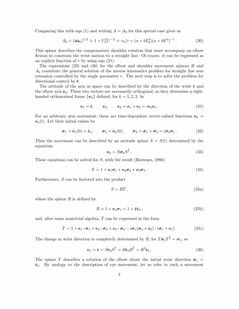
Comparing this with eqn (1) and writing A = A0 for this special case gives us

A0 = (aa0)1/2 = 1 + U20 U−2 = r0/r + (a + bE2

0)(a + bE2)−1 . (30)

This spinor describes the compensatory shoulder rotation that must accompany an elbowflexion to constrain the wrist motion to a straight line. Of course, it can be expressed asan explicit function of r by using eqn (21).

The expressions (23) and (30) for the elbow and shoulder movement spinors B andA0 constitute the general solution of the inverse kinematics problem for straight line armextension controlled by the single parameter r. The next step is to solve the problem fordirectional control by r.

The attitude of the arm in space can be described by the direction of the wrist r andthe elbow axis e2. These two vectors are necessarily orthogonal, so they determine a right-handed orthonormal frame {ek} defined, for k = 1, 2, 3, by

e1 = r, e2, e3 = e1 × e2 = ie2e1 . (31)

For an arbitrary arm movement, these are time-dependent vector-valued functions ek =ek(t). Let their initial values be

σ1 = e1(0) = r0, σ2 = e2(0), σ3 = σ1 × σ2 = iσ2σ1 . (32)

Then the movement can be described by an attitude spinor S = S(t) determined by theequations

ek = SσkS† . (33)

These equations can be solved for S, with the result (Hestenes, 1986)

S = 1 + e1σ1 + e2σ2 + e3σ3 . (34)

Furthermore, S can be factored into the product

S = RT , (35a)

where the spinor R is defined by

R = 1 + e1σ1 = 1 + rr0 , (35b)

and, after some nontrivial algebra, T can be expressed in the form

T = 1 + e1 · σ1 + e2 · σ2 + e3 · σ3 − iσ1(σ2 × e2) · (σ1 + e1) . (35c)

The change in wrist direction is completely determined by R, for Tσ1T† = σ1, so

e1 = r = Sr0S† = Rr0R

† = R2r0 . (36)

The spinor T describes a rotation of the elbow about the initial wrist direction σ1 =r0. By analogy to the description of eye movement, let us refer to such a movement

7

as reaching torsion. Torsion does not affect the wrist position, but it does affect thepositioning of the hand for grasping. Accordingly, the factoring of S into R and T ineqn (35a) can be interpreted as a factoring of arm movement into reaching and graspingsynergies. This mathematical representation should be helpful in empirical studies on thecoupling of reaching and grasping movements. For example, eqn (35c) tells us immediatelythat the condition

(σ2 × e2) · (σ1 + e1) = 0 (37)

is necessary and sufficient for pure reaching, so the empirical conditions under which itis fulfilled are worth studying. It might be expected to hold in pointing movements, forexample. In combined reaching and grasping movements, it would be of interest to comparethe temporal developments of R and T . There may be general neural rules governing torsionin reaching, just as there are in eye movement (Listing’s law), but they will undoubtedlydepend on what movement synergies are activated. Lacquanti and Soechting (1982) havealready found invariants coupling shoulder and elbow movement in experimental studies ofreaching.

The pieces can now be assembled to give the general solution to the inverse kinematicsproblem for reaching. For any arm movement from one posture to another, as described byeqn (4), the elbow flexion is described by the spinor B = B(r) in eqn (23) and the shoulderrotation is described by the spinor

A = SA0 = RTA0 , (38)

where A0 = A0(r) is given by eqn (30) and S, R, T are given by eqns (35a,b,c). Thissolution is expressed as a function of the target wrist position r factored into distancecontrol expressed by A0 = A0(r), B = B(r) and direction control expressed by R = R(r).This factorization is of interest if (or when) the nervous system employs r = | r | and r asmovement control variables, and it should be helpful for studying that possibility exper-imentally. However, if the nervous system employs different control variables, geometricalgebra should be just as helpful for analyzing their relation to the kinematics.

4. TRAJECTORY DESCRIPTION

In a reaching movement from an initial position r0 = r(t0) to a (final) target positionrf = r(tf ), the wrist follows a trajectory r = r(t) where t is the time or any other convenienttime parameter in the interval [ t0, tf ] (Figure 2). The solution of the inverse problem inSection 3 determines the joint spinors A, B, and A0 for each value of r(t) on the trajectory.The problem remains to describe the trajectory in terms of appropriate control parameters.The ultimate aim, of course, is to discover the control parameters employed by the centralnervous system. This can be facilitated by comparing alternative descriptions of trajectorykinematics with experimental data. Two such alternatives will be considered here: first, thefactorization of position into distance and direction; second, the factorization of velocityinto speed and direction.

The solution of the inverse kinematics problem in Section 3 suggests that factorizationof wrist position r into extension (or distance) r = | r | and direction r = n may be optimalfor computational purposes, because control of r = r(t) requires coordination of elbow and

8

r

Wrist

Shoulder

n0

n

rf

r

v = r

0ψ

0

shoulder joints, but control of n = n(t) in-volves only the shoulder. Accordingly, we write

r = rn . (39)

In terms of the independent variables r andn, the velocity v of the wrist is given by

v = r = rn + rn , (40)

where the overdot signifies time derivative. Therelation of n to n0 can be described by an an-gle ψ defined algebraically by

n = n0eIψ, (41)

where I is the unit bivector for the planeFIGURE 2. A wrist trajectory r=r(t) withvelocity v = r.

containing n and n0. If the wrist trajectory lies in a plane, then n is constant and differ-entiation of eqn (41) gives

n = nI ψ = −ψ In . (42)

Then eqn (40) can be expressed in the form of a complex variable:

vn = r + rnn = r − Ir ψ . (43)

Its modulus isv2 = v2 = r2 + r2n2 = r2 + r2ψ

2, (44)

where v = |v | is the speed of the wrist. Of course, the last equality in eqns (43) and (44)applies only to planar trajectories. The elementary relation (44) should be compared withexperimental data for possible evidence of independent control of r and n.

Morasso’s (1981) original finding that reaching trajectories are nearly straight lines withbell-shaped velocity profiles has been confirmed, extended, and refined by a number ofinvestigators (Abend, Bizzi, & Morasso, 1982: Atkeson & Hollerbach, 1985: Uno, Kawato& Suzuki, 1989). A minimal neural network model for generating such trajectories, theVITE model, has been developed by Bullock and Grossberg (1988). It is a purely kinematicmodel with endpoint control of velocity direction and independent speed control by a Gosignal. It is currently the most viable model of movement control because it is the simplest,and it accounts for the widest range of behavioral and neural data. The VITE model hasits limitations, however, as Bullock and Grossberg fully realize, but that is not of concernhere. Rather, we examine implications of the VITE model for coordinating direction anddistance control.

For radial trajectories, eqn (44) reduces to v2 = r2 so r must have a bell-shaped profile.From eqn (13), r is related to the elbow angle θ

r2 = a2 + b2 + 2ab cos θ . (45)

9

Differentiating this, we find

r =−θa sin θ

[ a2 + b2 + ab cos θ ]1/2, (46)

which shows that θ is certainly not bell-shaped when r is. lf a bell-shaped profile is thesignature of a movement control parameter, as the VITE model suggests, then r ratherthan θ is a candidate.

In the more general case, eqn (42) implies that if v and r are both bell-shaped, then rψmust be bell-shaped as well. This raises some interesting questions, because rψ combinesdistance and direction control variables. Any failure of perfect coordination between dis-tance and direction control would produce deviations from straight line trajectories as wellas anomalies in the rψ profile. The issue here is the expression of synergy formation in thekinematics of complex movements. Of course, there are other causes for deviations fromstraight line motion such as uncompensated forces and workspace boundaries. It shouldbe possible, however, to distinguish them experimentally from imperfect coordination ofdistance and direction control if, indeed, the issue is relevant to neural control.

Now we turn to the factorization of velocity into speed and direction and its kinematicimplications. This is an old topic that was thoroughly analyzed by differential geometersmore than a century ago. The aim here is to show how it can be simplified using geometricalgebra. This should be of practical value because the factorization is often employed inthe analysis of experimental data, and it may have theoretical significance.

The description of a smooth trajectory r = r(t) can be decomposed into a description ofthe geometrical path traversed and the distance traversed along the path by introducing apath length variable s = s(t). Accordingly, the velocity can be factored into

v = r = sr′ = vv , (47a)

where the speed is given byv = | r | = s , (47b)

and the velocity direction is given by

v = r′ =drds

, (47c)

the prime denoting differentiation with respect to path length.The geometry of the path can be described by specifying the derivatives of v in the fol-

lowing systematic way. A path-dependent orthonormal frame of vectors {ek = ek(s), k =1, 2, 3}, called a Frenet frame is introduced by identifying e1 with the path tangent vector

e1 = v = r′ , (48)

and defining the other vectors by the system of equations

e′1 = κe2,

e′2 = −κe1,+τ e3,

e′3 = −τ e2, (49)

10

where κ is a nonnegative scalar called the curvature of the path, and the scalar τ is calledthe torsion. By direct computation it can be shown that

κ = | r′′ | =| r × ..

r || r |3 =

|v × v ||v |3 . (50)

τ =(r′ × r′′) · r′′′

| r′′ |3 =(v × v) · ..

v|v × v |3 . (51)

The eqns (49) are the famous Frenet equations of classical differential geometry (Goetz,1970).

For a planar trajectory the torsion vanishes, and the geometrical shape of the path canbe described by the curvature κ = κ(t). From experimental data the curvature can bemeasured by evaluating the right side of (50). Then the trajectory can be described byexhibiting the speed and curvature profiles v = v(t) and κ = κ(t). This method fordescribing curved arm trajectories has been employed by Abend et al. (1982) and manyother researchers, particularly in the study of complex movements such as handwriting.

The description of arm trajectories by velocity and curvature profiles is certainly con-venient for experimental data analysis, but its theoretical significance is open to question.The basic theoretical question it raises is whether speed and velocity direction are subjectto independent control by the CNS. The VITE model asserts that they are for straightline trajectories. However, for curved trajectories they cannot be independently controlledbecause they are coupled dynamically. This suggests an important possibility that doesnot seem to have been mentioned in the literature heretofore, namely, that the tendencytoward straight line trajectories in reaching is a consequence of attempts by the CNS tofactor speed and direction control. This idea may be helpful in generalizing the adaptivefeatures of the VITE model.

Geometric algebra makes it possible to simplify the Frenet description of path geometrywith a method we have already employed for a different purpose (Hestenes, 1992). TheFrenet frame {ek} is completely determined by a spinor (quaternion)-valued function of thepath length F = F (s) through

ek = FσkF † , (52)

where F is normalized to FF † = 1 and, as before, {σk} is a conveniently chosen fixedorthonormal frame. The Frenet spinor must satisfy a differential equation of the form

F ′ = −12 iωDF , (53)

so differentiation of (52) yieldse′k = ωD × ek . (54)

The rotational velocity vector ωD for a Frenet frame is called the Darboux vector. Toexpress it in terms of curvature and torsion, we solve the three eqns (54) to get

ωD =12

3∑k=1

ek × e′k =12

3∑k=1

ek × e′k . (55)

Inserting eqn (49) into eqn (55) and using e3 = e1 × e2 = ie2e1, we obtain

ωD = κe3 + τ e1 (56)

11

or

ωD =v × v|v |3 +

(v × v) × (v × ..v)

(v × v)2|v | . (57)

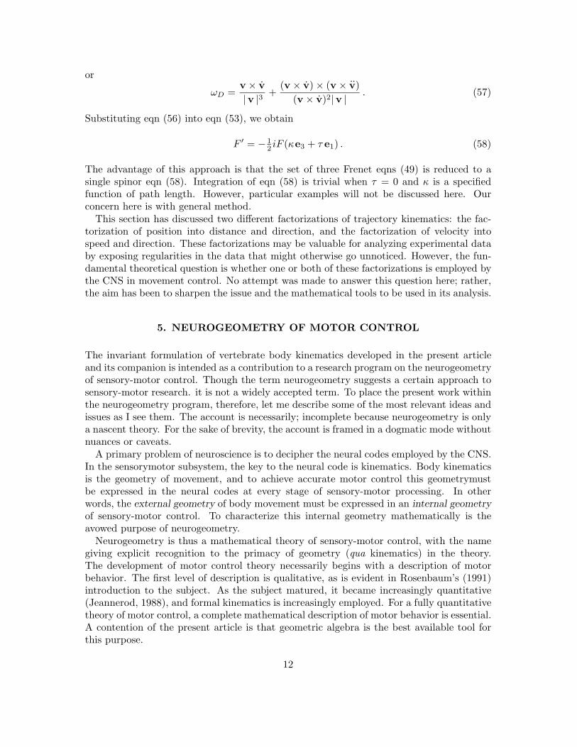
Substituting eqn (56) into eqn (53), we obtain

F ′ = −12 iF (κe3 + τ e1) . (58)

The advantage of this approach is that the set of three Frenet eqns (49) is reduced to asingle spinor eqn (58). Integration of eqn (58) is trivial when τ = 0 and κ is a specifiedfunction of path length. However, particular examples will not be discussed here. Ourconcern here is with general method.

This section has discussed two different factorizations of trajectory kinematics: the fac-torization of position into distance and direction, and the factorization of velocity intospeed and direction. These factorizations may be valuable for analyzing experimental databy exposing regularities in the data that might otherwise go unnoticed. However, the fun-damental theoretical question is whether one or both of these factorizations is employed bythe CNS in movement control. No attempt was made to answer this question here; rather,the aim has been to sharpen the issue and the mathematical tools to be used in its analysis.

5. NEUROGEOMETRY OF MOTOR CONTROL

The invariant formulation of vertebrate body kinematics developed in the present articleand its companion is intended as a contribution to a research program on the neurogeometryof sensory-motor control. Though the term neurogeometry suggests a certain approach tosensory-motor research. it is not a widely accepted term. To place the present work withinthe neurogeometry program, therefore, let me describe some of the most relevant ideas andissues as I see them. The account is necessarily; incomplete because neurogeometry is onlya nascent theory. For the sake of brevity, the account is framed in a dogmatic mode withoutnuances or caveats.

A primary problem of neuroscience is to decipher the neural codes employed by the CNS.In the sensorymotor subsystem, the key to the neural code is kinematics. Body kinematicsis the geometry of movement, and to achieve accurate motor control this geometrymustbe expressed in the neural codes at every stage of sensory-motor processing. In otherwords, the external geometry of body movement must be expressed in an internal geometryof sensory-motor control. To characterize this internal geometry mathematically is theavowed purpose of neurogeometry.

Neurogeometry is thus a mathematical theory of sensory-motor control, with the namegiving explicit recognition to the primacy of geometry (qua kinematics) in the theory.The development of motor control theory necessarily begins with a description of motorbehavior. The first level of description is qualitative, as is evident in Rosenbaum’s (1991)introduction to the subject. As the subject matured, it became increasingly quantitative(Jeannerod, 1988), and formal kinematics is increasingly employed. For a fully quantitativetheory of motor control, a complete mathematical description of motor behavior is essential.A contention of the present article is that geometric algebra is the best available tool forthis purpose.

12

A quantitative theory of motor control requires a quantitative model of what is controlled,namely, the vertebrate skeleto-muscular svstem. For kinematic purposes, this system canbe accurately modeled as system of N -linked rigid bodies. Because each rigid body hasthree rotational and three translational degrees of freedom, the configuration space of theentire system has dimension 6N . But if the linkages entail K constraints, then any possibleconfiguration is represented by a point on a (6N −K)-dimensional kinematic manifold (orsurface) in configuration space. Moreover, any body movement is a change in configuration,which can be described quantitatively as a curve on the kinematic manifold. This config-uration space description of body kinematics is an alternative to the more direct physicalspace description employed in this article, but it can also be efficiently expressed in termsof geometric algebra. However the body kinematics is described, it is an essential preludeto neurogeometry.

Neurogeometry begins with a description of the motor neuron signals for kinematic states(postures and/or movements) of the body. The description must be geometrical becausebody kinematics is geometrical. A valid description should make it possible to decipherempirically measured motor neuron signals, to interpret them geometrically as commandsto the muscles to produce particular kinematic states of the body.

Neurogeometry goes on to produce a neural network theory of sensory-motor controlin which every processing stage has geometrical interpretation specifying its relation tobody kinematics. Much neural network modeling that has already been published can bereinterpreted neurogeometrically. The most extensive and profound neural network theoryof sensory-motor control has been developed by Grossberg and his coworkers, Bullock andKuperstein. Their theory goes far beyond others in analyzing the implications of adaptiveconstraints and kinematic invariants. Moreover, it is compatible with the perspective ofneurogeometry.

Neural modeling is done at several different levels of biological organization (Shepherd,1990). The level at which a geometric interpretation is most appropriate could well becalled the psychophysical level. At that level sensory-motor information is encoded inactivity patterns across neuronal populations (Hestenes, 1991b). This is presumed in thefollowing discussion.

5.1. PPC and Self-Calibration

When the body is maintaining a particular posture, the pattern of neural command signalsto the muscles constitute a representation of posture called the present position command(PPC) by Bullock and Grossberg (1988). It has often been argued that, for rapid and accu-rate movement, the PPC must also be employed as an efferent copy (or corollary discharge)in internal computations. One reason for this is that afferent measurements of postureare too slow to track rapid movements, so the best available alternative is to employ thePPC predictively during movement. However, that raises a serious self-calibration problem,first subjected to a detailed analysis by Grossberg and Kuperstein (1989). They note thatmuscle length is a highly nonlinear function of the neural command signals and argue thatthis functional relation must be linearized by recalibration to compensate for inevitablechanges in muscle performance due to injury, growth, and so on. However, they tacitlyassume that muscle length is the preferred parametrization of posture, though their argu-

13

ment suffices to prove that muscle contraction can be linearly calibrated to any convenientparameter. Neurogeometry suggests alternatives. For example, our kinematic analysis ofreaching suggests that arm extension is a behaviorally more significant variable than el-bow angle (which corresponds closely to muscle length). Moreover, it is quite possible, ifnot likely, that the contractions of a given muscle have different calibrations depending onwhich movement synergy is engaged. Note that such adaptive rescaling changes the neuralcode or, as Pellionisz and Linas (1985) would say, changes the metric of the neurogeometry.

5.2. Kinematic Invariants and Motor Synergies

A motor (or muscle) synergy is a coordinated action of muscle groups to produce a sin-gle class of gestures. Synergy formation reduces the number of degrees of freedom amongthe muscles involved, and this is reflected in the existence of kinematic invariants of thegestures. For example, Listing’s law describes an invariant of saccadic eye movements. Aswe have noted, such invariants characterize the constraints on a synergy and so provideclues about the neural variables controlling the synergy. Neurogeometry seeks to describethe neural control variables geometrically to make the connection with the kinematics ofmovement explicit. Synergy formation is a self-organization process that can be describedgeometrically as the formation of a kinematic manifold in configuration space. A gesturecan then be described as a curve on that manifold, a curve with specified endpoints. Ac-cording to neurogeometry, for given endpoints the curve is determined by the geometry ofthe manifold, in much the same way as particle histories are determined by spacetime geom-etry in Einstein’s General Theory of Relativity. However, neurogeometry is not developedsufficiently to supply an equally complete mathematical formulation.

Bullock and Grossberg (1991) propose a kinematic invariant of reaching gestures calledposition code invariance, which asserts that the path of a given gesture is invariant underboth speed and stiffness rescaling. This is to say that the same gesture can be performedat different speeds and muscle stiffness levels. As noted in the preceding section, the VITEmodel is designed to exhibit speed rescaling invariance. but that is difficult to achievefor curved trajectories. The outstanding feature of the VITE model is that the movementcontrol variables are purely kinematical. To preserve this feature when generalizing theVITE model to accommodate independent muscle stiffness control. Grossberg and Bullock(1991) developed the FLETE model, which explains how stiffness rescaling invariance canbe implemented in a biologically plausible neural network. Muscle stiffness control can beinterpreted geometrically as sculpting a valley around the movement trajectory to stabilizeit against perturbing external forces. A detailed review of experimental evidence for suchtrajectory stabilization is given by Bizzi and Mussa-Ivaldi (1990). The main idea in allthis is that neural motor control can be described geometrically even under the influenceof perturbing forces. Thus, in motor control, dynamics is reduced to kinematics!

These qualitative remarks serve only to provide a neurogeometric perspective for integrat-ing the present work on body kinematics with the neural motor control theory of Bullock,Grossberg and Kuperstein. Their rich theory contains a mathematical formulation andanalysis of many more important network principles and designs, such as designs for invari-ant target maps. The emphasis here is on the primacy of perceptual geometry and bodykinematics for determining the constraints on neural network designs. More specifically, the

14

present work is intended to demonstrate the value of geometric algebra for mathematicalformulation and analysis of these design constraints.

It is enlightening to compare the neurogeometry research program with Newton’s originalprogram for developing mechanics (Hestenes, 1992). In the preface to his great Principia,Newton concluded that his approach to research can be reduced to this: from the motionsof bodies (kinematics) infer the forces, and from the forces deduce the motions (dynamics).This iterative cycle of quantitative kinematical description coupled with dynamical model-ing and testing has been employed by physicists for three centuries with incredible successto discover the fundamental forces of nature.

Similarly, the neurogeometry approach is to quantify the kinematics of body movement(including adaptive changes in kinematics) to ascertain constraints on motor control designs,then to develop neurally plausible models of sensory-motor control that can be testedempirically. The goal of neurogeometry can be described as deciphering the neural sensory-motor code. Analogously, Newton’s goal could be described as deciphering the code ofphysical motions to discover hidden physical forces. Indeed, Galileo described the goal ofscience (philosophy) in precisely these terms (translation from Burtt, 1932):“Philosophy is written in that great book which ever lies before our eyes—I mean theUniverse—but we cannot understand it if we do not first learn the language and grasp thesymbols in which it is written. This book is written in the mathematical language, andthe symbols are triangles, circles, and other geometrical figures, without whose help it isimpossible to comprehend a single word of it; without which one wanders in vain througha dark labyrinth.”

REFERENCES

Abend, W., Bizzi, E., & Morasso, P. (1982). Human arm trajectory formation. Brain. 105,331-348.

Atkeson, C., & Hollerback, J. (1985). Kinematic features of unrestrained vertical arm move-ments. Journal of Neuroscience. 5, 2318–2330.

Bizzi, E., & Mussa-Ivaldi, F. (1990). Muscle properties and the control of movement. In D.Osherson, S. Kosslyn, & J. Hollerback (Eds.), Visual cognition and action (Vol. 2, pp.213–242). Cambridge: MIT Press.

Bullock, D., & Grossberg, S. (1988). Neural dynamics of planned arm movements: Emergentinvariants and speed-accuracy properties during planned arm movements. PsychologicalReview, 95, 49–90.

Bullock, D., & Grossberg, S. (1991). Adaptive neural networks for control of movementtrajectories invariant under speed and force rescaling. Human Movement Science, 10,3–53.

Burtt, E. A. (1932). The metaphysical foundations of modern science (p. 67). London:Routledge and Kegen Paul Ltd.

Goetz, H. (1970). Introduction to differential geometry (chap. 2). New York: Addison-Wesley.

Grossberg, S., & Kuperstein, M. (1989). Neutral dynamics of adaptive sensory motor con-trol: Expanded edition. New York: Pergamon.

15

Hestenes, D. (1986). New foundations for classical mechanics. Dordrecht: Kluwer (4th printingwith corrections, 1992).

Hestenes, D. (1991a). The design of linear algebra and geometry. Acta Mathematical Ap-plicandea. 23, 65–93.

Hestenes, D. (1991b). A cardinal principle of neuropsychology, with implications for schizo-phrenia and mania. Behavioral and Brain Sciences. 14, 31–32.

Hestenes, D. (1992). Modeling games in the Newtonian world. American Journal of Physics.60, 732–748.

Hestenes, D. (1993). Invariant body kinematics I: Saccadic and compensatory eye move-ments. Neural Networks. 7, 65–77.

Hollerbach, J., & Flash, T. (1982). Dynamic interactions between limb segments duringplanar arm movements. Biological Cybernetics. 44, 67–77.

Jennerod, M. (1988). The neural and behavioral organization of goal-directed movements.New York: Oxford University Press.

Lacquanti, F., & Soechting, J. (1982). Coordination of arm and wrist motion during areaching task. Journal of Neuroscience. 2 399–408.

Morasso, P. (1981). Spatial control of arm movements. Experimental Brain Research. 42,223–227.

Pellionisz, A., & Llinas, R. (1980). Tensorial approach to the geometry of brain function:Cerebellar coordination via metric tensor. Neuroscience, 5, 1125–1136.

Pellionisz, A., & Llinas, R. (1985). Tensor network theory of the metaorganization of func-tional geometries in the nervous system. Neuroscience, 16, 245–273.

Rosenbaum, D. A. (1991). Human motor control. an Diego: Academic Press.

Shepherd, G. M. (1990). The significance of real neuron architectures for neural networksimulations. In E. L. Schwartz (Ed.) Computational neuroscience (pp. 82-96). Cam-bridge: MIT Press.

Soechting, J., & Lacquanti, F. (1981). Invariant characteristics of pointing in man. Journal

of Neuroscience. 1, 710–720.

Spong, M., & Vidyasagar, M. (1989). Robot dynamics and control. New York: Wiley.

Uno., Y., Kawato, & Suzuki, R. (1989). Formation and control of optimal trajectory. Bio-logical Cybernetics. 61, 89–101.

APPENDIX: EUCLIDEAN HYPERSPINORS FOR KlNEMATlC CHAINS

As shown in several references, the geometric algebra employed in this article has richgeneralizations to multilinear spaces and manifolds of arbitrary dimension. This appendixcalls attention to one little-known generalization that may prove to be especially valuablefor describing and analyzing complex body kinematics.

A sequence of rotations and translations is called a kinematic chain in robotic theory(Spong & Vidyasagar, 1989). The variable position of any point on the body can bedescribed by a parametrized kinematic chain. Thus, the position vector f of a finger tipis described by a kinematic chain in eqn (7). We have noted how such a description is

16

simplified by the spinor representation of rotations. Further simplification can be achievedby introducing a similar representation for translations.

Let x be the position vector for a generic point on a body in Euclidean 3-space. Withgeometric algebra, any rigid displacement f of the body can be written in the form

x → f(x) = R(x + a0)R† = RxR† + a , (A.1)

expressing it as a rotation determined by a unimodular spinor R preceded by a translationby the vector a0 or followed by a translation by

a = Ra0R† . (A.2)

The drawback with eqn (A.1) is that rotations combine multiplicatively and translationscombine additively. Translations as well as rotations can be expressed multiplicatively bythe following artifice.

We introduce a new algebraic entity ε, which has the null property

ε2 = 0 (A.3)

and commutes with vectors, that is,εa = aε (A.4)

for every vector a. The translation by a can be represented by a hyperspinor Ta defined by

Ta = e12aε = 1 + 1

2aε . (A.5)

Note that the power series expansion of the exponential function in eqn (A.5) is terminatedby the fact that ε2 = 0.

The rigid displacement f defined by eqn (A.1) can now be represented more compactlyby a hyperspinor F defined by

F = TaR = RTa0 . (A.6)

Assuming thatε† = ε (A.7)

soTaT

†a = T 2

a = T2a = 1 + εa , (A.8)

the relation of f to F can be described by the equation

F (1 + xε)F † = 1 + f(x)ε . (A.9)

That is all there is to it!The advantage of using hyperspinors to represent rigid displacements is that the com-

position of arbitrary displacements is reduced to multiplication. Thus, for displacementsrepresented by F1 and F2, the composite is given by

F3 = F2F1 . (A.10)

17

Each Fi can be factored into a rotation followed by a translation, as expressed by

Fi = TaiRi . (A.11)

Accordingly, from eqn (A.10) it follows easily that

R3 = R2R1 (A.12a)

anda3 = a2 + R2a1R

†2 . (A.12b)

Thus, the translational and rotational factors of the composite transformation can be com-puted directly without referring to the action on a body point x as eqn (A.1) does.

The set of all rigid displacements form a mathematical group sometimes called the Eu-clidean group. Equation (A.9) establishes that hyperspinors defined by eqn (A.6) are repre-sentations of the Euclidean group. [Actually, the representations are double-valued, becauseeqn (A.9) is invariant under replacement of F by −F . The significance of this detail is ex-plained in Section 5-3 of Hestenes (1986).] Equation (A.10) is the basis group propertyexpressed in terms of hyperspinors. The special power of this representation comes fromthe structure of geometric algebra.

As an illustrative application to body kinematics, the kinematic chain determining thevector f in eqn (7) can now be represented by a hyperspinor

F = ATa0BTb0CTc0 . (A.13)

It follows from eqn (A.9) that f is determined by

FF † = 1 + fε , (A.14)

from which eqn (7) can be derived. This suffices to show how any kinematic chain can berepresented multiplicatively by hyperspinors and related to the vectorial form.

It remains to be seen how valuable hyperspinors will be for modeling complex bodykinematics. Though some evidence has been noted in the preceding paper (Hestenes, 1992b)that the CNS may, in effect, employ spinors in its computations, the possibility that italso employs hyperspinors seems utterly remote. That should not gainsay, however, thevalue of hyperspinors for the mathematical description and analysis of motor behavior.Howeover, the efficiency of designs for robotic control might be optimized by incorporatinghyperspinors.

The basic eqns (A.6) and (A.9) for the hyperspinor representation of the Euclideangroup were derived by Hestenes (1991a) from a much more general mathematical contentwith a richer group structure—including reflections, inversions, and dilatations in spacesof arbitrary dimension and signature. It is shown there that the quantity in this appendixcan be interpreted geometrically as a null vector in a space of higher dimension. Thoughall of that supplies a powerful mathematical perspective with many other applications, itis not clear that it can enhance the mathematical treatment of body kinematics.

18