inventory and monitoring technical reference 1734–7
TRANSCRIPT

INVENTORY AND MONITORINGTechnical Reference 1734–7
Ecological Site Inventory
December 2001
U.S. Department of the Interior • Bureau of Land Management

Copies available from:
Bureau of Land Management National Business Center
Printed Materials Distribution Services (BC-650B)P.O. Box 25047
Denver, Colorado 80225-0047
BLM/ST/ST-01/003+1734
This document is also available on the NSTC Web site at http://www.blm.gov/nstc
Production services provided by:
Information and Communications StaffTerry D’Erchia, Chief (303-236-6547)
Janine Koselak: Layout and DesignKathy Rohling: Editing
Lee Barkow, DirectorNational Science & Technology CenterP.O. Box 25047Denver, Colorado 80225-0047
The Bureau of Land Management’s National Scienceand Technology Center supports other BLM offices byproviding a broad spectrum of services in areas such asphysical, biological, and social science assessments;architecture and engineering support; library assis-tance; mapping science; photo imaging; geographicinformation systems applications; and publicationssupport.
INVENTORY AND MONITORINGTechnical Reference 1734–7
Ecological Site Inventory
December 2001
By:
Edward F. Habich
Rangeland Management Specialist
Bureau of Land Management
National Science and Technology Center
Denver, Colorado
U.S. Department of the Interior • Bureau of Land Management

“An ecological site is a distinctive kind of land with specific
physical characteristics that differs from others kinds of land in its
ability to produce a distinctive kind and amount of vegetation.”
–National Range and Pasture Handbook
Suggested citation:
Habich, E.F. 2001. Ecological site inventory, Technical reference 1734-7. Bureau of Land Management.Denver, Colorado. BLM/ST/ST-01/003+1734. 112 pp.

S
INVENTORY AND MONITORING Technical Reference 1734–7 • Ecological Site Inventory
Prefacei
PrefaceSINCE DECEMBER 1982, ecological siteinventory (ESI) has been the Bureau of LandManagement’s (BLM) standard vegetation inven-tory technique. The ecological site inventorymethod involves the use of soils information tomap ecological sites and plant communities andthe collection of natural resource and vegetationattributes. The sampling data from each of thesesoil-vegetation units, referred to as site write-upareas (SWAs), become the baseline data fornatural resource management and planning.
The purpose of Technical Reference 1734-7,Ecological Site Inventory, is to identify the proce-dures for completing an ecological site inventoryand to describe the technique used by theNatural Resource Conservation Service (NRCS)to document and describe ecological sites. Theseprocedures were derived from the NRCS
Rangeland Ecological Site Inventory procedureas described in their National Range and PastureHandbook. Information was also adapted fromthe NRCS National Soils Handbook and BLMTechnical Reference 1737-7, Procedures forEcological Site Inventory—With Special Reference toRiparian-Wetland Sites. Technical Reference 1734-7replaces previous guidance found in BLMManual Handbook 4410-1.
The need for natural resource inventories aremandated by Congress in Section 201(a) of theFederal Land Policy and Management Act(FLPMA) of 1976. Congress reaffirmed this needin Section 4 of the Public RangelandsImprovement Act (PRIA) of 1978—in particular,to develop and maintain an inventory of rangeconditions and trends on public rangelands, andto keep that inventory updated on a regular basis.

INVENTORY AND MONITORING Technical Reference 1734–7 • Ecological Site Inventory
Table of Contentsiii
Table of ContentsPreface . . . . . . . . . . . . . . . . . . . . . . . . . . . . . . . . . . . . . . . . . . . . . . . . . . . . . . . . . . . . . . . . . . . . . . .i
Chapter 1 - Inventory . . . . . . . . . . . . . . . . . . . . . . . . . . . . . . . . . . . . . . . . . . . . . . . . . . . . . . . . . .1Inventory Preparation . . . . . . . . . . . . . . . . . . . . . . . . . . . . . . . . . . . . . . . . . . . . . . . . . . . . . . . . .1
Inventory Plan. . . . . . . . . . . . . . . . . . . . . . . . . . . . . . . . . . . . . . . . . . . . . . . . . . . . . . . . . . . .1Table 1 - Inventory Plan Format . . . . . . . . . . . . . . . . . . . . . . . . . . . . . . . . . . . . . . . . . . . .2
Inventory Plan Reviews . . . . . . . . . . . . . . . . . . . . . . . . . . . . . . . . . . . . . . . . . . . . . . . . . . . .4Inventory Team . . . . . . . . . . . . . . . . . . . . . . . . . . . . . . . . . . . . . . . . . . . . . . . . . . . . . . . . . .4
Figure 1 - Composition of Inventory Team . . . . . . . . . . . . . . . . . . . . . . . . . . . . . . . . . . . . . .4Team Lead . . . . . . . . . . . . . . . . . . . . . . . . . . . . . . . . . . . . . . . . . . . . . . . . . . . . . . . . . . .5Soil Survey Team . . . . . . . . . . . . . . . . . . . . . . . . . . . . . . . . . . . . . . . . . . . . . . . . . . . . . .5Vegetation Mapping Team . . . . . . . . . . . . . . . . . . . . . . . . . . . . . . . . . . . . . . . . . . . . . . .5Vegetation Transecting Team . . . . . . . . . . . . . . . . . . . . . . . . . . . . . . . . . . . . . . . . . . . . .5Phenological Data Collection Team . . . . . . . . . . . . . . . . . . . . . . . . . . . . . . . . . . . . . . . .5Natural Resource Specialists on the Inventory Team . . . . . . . . . . . . . . . . . . . . . . . . . . .5
Preparing for Field Operations . . . . . . . . . . . . . . . . . . . . . . . . . . . . . . . . . . . . . . . . . . . . . . . . . .7Training and Orientation . . . . . . . . . . . . . . . . . . . . . . . . . . . . . . . . . . . . . . . . . . . . . . . . . . .7Aerial Photographs and Maps . . . . . . . . . . . . . . . . . . . . . . . . . . . . . . . . . . . . . . . . . . . . . . .8
Aerial Photographs . . . . . . . . . . . . . . . . . . . . . . . . . . . . . . . . . . . . . . . . . . . . . . . . . . . . .8Orthophoto Quads . . . . . . . . . . . . . . . . . . . . . . . . . . . . . . . . . . . . . . . . . . . . . . . . . . . .8Topographic and Planimetric Maps . . . . . . . . . . . . . . . . . . . . . . . . . . . . . . . . . . . . . . . .8Administrative Maps . . . . . . . . . . . . . . . . . . . . . . . . . . . . . . . . . . . . . . . . . . . . . . . . . . .9Other Maps . . . . . . . . . . . . . . . . . . . . . . . . . . . . . . . . . . . . . . . . . . . . . . . . . . . . . . . . . .9Remote Sensing Imagery . . . . . . . . . . . . . . . . . . . . . . . . . . . . . . . . . . . . . . . . . . . . . . . .9
General Equipment . . . . . . . . . . . . . . . . . . . . . . . . . . . . . . . . . . . . . . . . . . . . . . . . . . . . . . .9Table 2 - Equipment List . . . . . . . . . . . . . . . . . . . . . . . . . . . . . . . . . . . . . . . . . . . . . . . . .10
Specialized Equipment . . . . . . . . . . . . . . . . . . . . . . . . . . . . . . . . . . . . . . . . . . . . . . . . . . . .11Soils . . . . . . . . . . . . . . . . . . . . . . . . . . . . . . . . . . . . . . . . . . . . . . . . . . . . . . . . . . . . . . .11Vegetation . . . . . . . . . . . . . . . . . . . . . . . . . . . . . . . . . . . . . . . . . . . . . . . . . . . . . . . . . .11Wildlife Biology . . . . . . . . . . . . . . . . . . . . . . . . . . . . . . . . . . . . . . . . . . . . . . . . . . . . . .12Hydrology . . . . . . . . . . . . . . . . . . . . . . . . . . . . . . . . . . . . . . . . . . . . . . . . . . . . . . . . . .12
Chapter 2 - Soils . . . . . . . . . . . . . . . . . . . . . . . . . . . . . . . . . . . . . . . . . . . . . . . . . . . . . . . . . . . . .15Soil Map Unit . . . . . . . . . . . . . . . . . . . . . . . . . . . . . . . . . . . . . . . . . . . . . . . . . . . . . . . . . . . . . .15
Consociation . . . . . . . . . . . . . . . . . . . . . . . . . . . . . . . . . . . . . . . . . . . . . . . . . . . . . . . . . . .15Complex . . . . . . . . . . . . . . . . . . . . . . . . . . . . . . . . . . . . . . . . . . . . . . . . . . . . . . . . . . . . . . .15Association . . . . . . . . . . . . . . . . . . . . . . . . . . . . . . . . . . . . . . . . . . . . . . . . . . . . . . . . . . . . .15Undifferentiated Group . . . . . . . . . . . . . . . . . . . . . . . . . . . . . . . . . . . . . . . . . . . . . . . . . . .16
Soil Map Unit Development . . . . . . . . . . . . . . . . . . . . . . . . . . . . . . . . . . . . . . . . . . . . . . . . . . .16

INVENTORY AND MONITORING Technical Reference 1734–7 • Ecological Site Inventory
Table of Contentsiv
Soil Map Unit Descriptions . . . . . . . . . . . . . . . . . . . . . . . . . . . . . . . . . . . . . . . . . . . . . . . . . . .16Detailed Soil Maps . . . . . . . . . . . . . . . . . . . . . . . . . . . . . . . . . . . . . . . . . . . . . . . . . . . . . . . . . .16Soil Survey Mapping for Riparian-Wetland Areas . . . . . . . . . . . . . . . . . . . . . . . . . . . . . . . . . .17
Figure 2 - Schematic Representation of Soil Map with Line Segments . . . . . . . . . . . . . . . . . . . .17Importance of Soil Map Units . . . . . . . . . . . . . . . . . . . . . . . . . . . . . . . . . . . . . . . . . . . . . . . . .18
Chapter 3 - Ecological Sites . . . . . . . . . . . . . . . . . . . . . . . . . . . . . . . . . . . . . . . . . . . . . . . . . . . .19Definition of Ecological Site . . . . . . . . . . . . . . . . . . . . . . . . . . . . . . . . . . . . . . . . . . . . . . . . . . .19Succession and Retrogression . . . . . . . . . . . . . . . . . . . . . . . . . . . . . . . . . . . . . . . . . . . . . . . . . .19States and Transition Pathways . . . . . . . . . . . . . . . . . . . . . . . . . . . . . . . . . . . . . . . . . . . . . . . .20
Figure 3 - State and Transition Model Diagram for an Ecological Site . . . . . . . . . . . . . . . . . . . .20Historic Climax Plant Community . . . . . . . . . . . . . . . . . . . . . . . . . . . . . . . . . . . . . . . . . . . . . .22Naturalized Plant Community . . . . . . . . . . . . . . . . . . . . . . . . . . . . . . . . . . . . . . . . . . . . . . . . .22Potential Natural Community . . . . . . . . . . . . . . . . . . . . . . . . . . . . . . . . . . . . . . . . . . . . . . . . .23Historic Climax Plant Community Versus Potential Natural Community . . . . . . . . . . . . . . . .23Changes in Ecological Site Potential . . . . . . . . . . . . . . . . . . . . . . . . . . . . . . . . . . . . . . . . . . . . .23Characteristic Vegetation States of an Ecological Site . . . . . . . . . . . . . . . . . . . . . . . . . . . . . . .24Differentiation Between Ecological Sites . . . . . . . . . . . . . . . . . . . . . . . . . . . . . . . . . . . . . . . . .24Revising Ecological Site Descriptions . . . . . . . . . . . . . . . . . . . . . . . . . . . . . . . . . . . . . . . . . . . .26Developing New Ecological Site Descriptions . . . . . . . . . . . . . . . . . . . . . . . . . . . . . . . . . . . . .26BLM Procedures . . . . . . . . . . . . . . . . . . . . . . . . . . . . . . . . . . . . . . . . . . . . . . . . . . . . . . . . . . . .26Naming Ecological Sites on Rangeland . . . . . . . . . . . . . . . . . . . . . . . . . . . . . . . . . . . . . . . . . . .26Numbering Ecological Sites . . . . . . . . . . . . . . . . . . . . . . . . . . . . . . . . . . . . . . . . . . . . . . . . . . .27Correlating Ecological Sites . . . . . . . . . . . . . . . . . . . . . . . . . . . . . . . . . . . . . . . . . . . . . . . . . . .28Ecological Site Description . . . . . . . . . . . . . . . . . . . . . . . . . . . . . . . . . . . . . . . . . . . . . . . . . . . .28
Heading . . . . . . . . . . . . . . . . . . . . . . . . . . . . . . . . . . . . . . . . . . . . . . . . . . . . . . . . . . . . . . .28Ecological Site Name . . . . . . . . . . . . . . . . . . . . . . . . . . . . . . . . . . . . . . . . . . . . . . . . . . . . .28Ecological Site ID . . . . . . . . . . . . . . . . . . . . . . . . . . . . . . . . . . . . . . . . . . . . . . . . . . . . . . . .28Major Land Resource Area . . . . . . . . . . . . . . . . . . . . . . . . . . . . . . . . . . . . . . . . . . . . . . . . .28Interstate Correlation . . . . . . . . . . . . . . . . . . . . . . . . . . . . . . . . . . . . . . . . . . . . . . . . . . . . .28Physiographic Features . . . . . . . . . . . . . . . . . . . . . . . . . . . . . . . . . . . . . . . . . . . . . . . . . . . .28Climatic Features . . . . . . . . . . . . . . . . . . . . . . . . . . . . . . . . . . . . . . . . . . . . . . . . . . . . . . . .29Influencing Water Features . . . . . . . . . . . . . . . . . . . . . . . . . . . . . . . . . . . . . . . . . . . . . . . . .29Representative Soil Features . . . . . . . . . . . . . . . . . . . . . . . . . . . . . . . . . . . . . . . . . . . . . . . .29Ecological Dynamics of the Site . . . . . . . . . . . . . . . . . . . . . . . . . . . . . . . . . . . . . . . . . . . . .29Plant Communities . . . . . . . . . . . . . . . . . . . . . . . . . . . . . . . . . . . . . . . . . . . . . . . . . . . . . . .29Species List . . . . . . . . . . . . . . . . . . . . . . . . . . . . . . . . . . . . . . . . . . . . . . . . . . . . . . . . . . . . .30Plant Groups . . . . . . . . . . . . . . . . . . . . . . . . . . . . . . . . . . . . . . . . . . . . . . . . . . . . . . . . . . . .30Cover and Structure . . . . . . . . . . . . . . . . . . . . . . . . . . . . . . . . . . . . . . . . . . . . . . . . . . . . . .31
Table 3 - Cover and Structure . . . . . . . . . . . . . . . . . . . . . . . . . . . . . . . . . . . . . . . . . . . . .31Biological Soil Crust Communities . . . . . . . . . . . . . . . . . . . . . . . . . . . . . . . . . . . . . . . . . .32Total Annual Production . . . . . . . . . . . . . . . . . . . . . . . . . . . . . . . . . . . . . . . . . . . . . . . . . .32

INVENTORY AND MONITORING Technical Reference 1734–7 • Ecological Site Inventory
Table of Contentsv
Plant Community Growth Curves . . . . . . . . . . . . . . . . . . . . . . . . . . . . . . . . . . . . . . . . . . .32Table 4 - Plant Community Growth Curves . . . . . . . . . . . . . . . . . . . . . . . . . . . . . . . . . . .32
Ecological Site Interpretations . . . . . . . . . . . . . . . . . . . . . . . . . . . . . . . . . . . . . . . . . . . . . .32Animal Community . . . . . . . . . . . . . . . . . . . . . . . . . . . . . . . . . . . . . . . . . . . . . . . . . . .32Hydrologic Functions . . . . . . . . . . . . . . . . . . . . . . . . . . . . . . . . . . . . . . . . . . . . . . . . . .33Recreational Uses . . . . . . . . . . . . . . . . . . . . . . . . . . . . . . . . . . . . . . . . . . . . . . . . . . . . .33Wood Products . . . . . . . . . . . . . . . . . . . . . . . . . . . . . . . . . . . . . . . . . . . . . . . . . . . . . . .33Other Products . . . . . . . . . . . . . . . . . . . . . . . . . . . . . . . . . . . . . . . . . . . . . . . . . . . . . . .33Supporting Information . . . . . . . . . . . . . . . . . . . . . . . . . . . . . . . . . . . . . . . . . . . . . . . .33Associated Sites . . . . . . . . . . . . . . . . . . . . . . . . . . . . . . . . . . . . . . . . . . . . . . . . . . . . . .33Similar Sites . . . . . . . . . . . . . . . . . . . . . . . . . . . . . . . . . . . . . . . . . . . . . . . . . . . . . . . . .33Inventory Data References . . . . . . . . . . . . . . . . . . . . . . . . . . . . . . . . . . . . . . . . . . . . . .33State Correlation . . . . . . . . . . . . . . . . . . . . . . . . . . . . . . . . . . . . . . . . . . . . . . . . . . . . .33Type Locality . . . . . . . . . . . . . . . . . . . . . . . . . . . . . . . . . . . . . . . . . . . . . . . . . . . . . . . .33Relationship to Other Established Classification Systems . . . . . . . . . . . . . . . . . . . . . .33Other References . . . . . . . . . . . . . . . . . . . . . . . . . . . . . . . . . . . . . . . . . . . . . . . . . . . . .33
Ecological Site Documentation and References . . . . . . . . . . . . . . . . . . . . . . . . . . . . . . . . .33Authorship . . . . . . . . . . . . . . . . . . . . . . . . . . . . . . . . . . . . . . . . . . . . . . . . . . . . . . . . . .34Site Approval . . . . . . . . . . . . . . . . . . . . . . . . . . . . . . . . . . . . . . . . . . . . . . . . . . . . . . . .34
Forestland Ecological Sites . . . . . . . . . . . . . . . . . . . . . . . . . . . . . . . . . . . . . . . . . . . . . . . . . . . .34Separating Forested Lands from Rangelands in Areas Where They Interface . . . . . . . . . . . . .34
Chapter 4 - Production Data . . . . . . . . . . . . . . . . . . . . . . . . . . . . . . . . . . . . . . . . . . . . . . . . . . .35Aboveground Vegetation Production . . . . . . . . . . . . . . . . . . . . . . . . . . . . . . . . . . . . . . . . . . . .35Total Annual Production . . . . . . . . . . . . . . . . . . . . . . . . . . . . . . . . . . . . . . . . . . . . . . . . . . . . . .35Production for Various Kinds of Plants . . . . . . . . . . . . . . . . . . . . . . . . . . . . . . . . . . . . . . . . . . .35
Herbaceous Plants . . . . . . . . . . . . . . . . . . . . . . . . . . . . . . . . . . . . . . . . . . . . . . . . . . . . . . .36Woody Plants . . . . . . . . . . . . . . . . . . . . . . . . . . . . . . . . . . . . . . . . . . . . . . . . . . . . . . . . . . .36Cacti . . . . . . . . . . . . . . . . . . . . . . . . . . . . . . . . . . . . . . . . . . . . . . . . . . . . . . . . . . . . . . . .36
Methods of Determining Production . . . . . . . . . . . . . . . . . . . . . . . . . . . . . . . . . . . . . . . . . . . .37Figure 4 - Weight Estimate Plots . . . . . . . . . . . . . . . . . . . . . . . . . . . . . . . . . . . . . . . . . . . . . . .37
Estimating by Weight Units . . . . . . . . . . . . . . . . . . . . . . . . . . . . . . . . . . . . . . . . . . . . . . . . . . .38Double Sampling—Estimating and Harvesting . . . . . . . . . . . . . . . . . . . . . . . . . . . . . . . . . . . .39
Table 5 - Number of Harvested Plots . . . . . . . . . . . . . . . . . . . . . . . . . . . . . . . . . . . . . . . . . . .39Plot Size . . . . . . . . . . . . . . . . . . . . . . . . . . . . . . . . . . . . . . . . . . . . . . . . . . . . . . . . . . . . . . .40Plot Shape . . . . . . . . . . . . . . . . . . . . . . . . . . . . . . . . . . . . . . . . . . . . . . . . . . . . . . . . . . . . . .40
Harvesting . . . . . . . . . . . . . . . . . . . . . . . . . . . . . . . . . . . . . . . . . . . . . . . . . . . . . . . . . . . . . . . .41Units of Production and Conversion Factors . . . . . . . . . . . . . . . . . . . . . . . . . . . . . . . . . . . . . .41Plot Size Conversion Factors . . . . . . . . . . . . . . . . . . . . . . . . . . . . . . . . . . . . . . . . . . . . . . . . . .41
Table 6 - Conversion Factors for Grams to Pounds per Acre . . . . . . . . . . . . . . . . . . . . . . . . . . .41Table 7 - Conversion Factors for Grams to Kilograms per Hectare . . . . . . . . . . . . . . . . . . . . . . .42Mixed Measuring Units . . . . . . . . . . . . . . . . . . . . . . . . . . . . . . . . . . . . . . . . . . . . . . . . . . .42

INVENTORY AND MONITORING Technical Reference 1734–7 • Ecological Site Inventory
Table of Contentsvi
Adjustment Factors . . . . . . . . . . . . . . . . . . . . . . . . . . . . . . . . . . . . . . . . . . . . . . . . . . . . . . . . . .42Green Weight Adjustment Factor . . . . . . . . . . . . . . . . . . . . . . . . . . . . . . . . . . . . . . . . . . . .42Double Sampling Adjustment Factor . . . . . . . . . . . . . . . . . . . . . . . . . . . . . . . . . . . . . . . . .43Air-dry Weight Adjustment Factor . . . . . . . . . . . . . . . . . . . . . . . . . . . . . . . . . . . . . . . . . . .43Utilization Adjustment Factor . . . . . . . . . . . . . . . . . . . . . . . . . . . . . . . . . . . . . . . . . . . . . .43Growth Adjustment Factor . . . . . . . . . . . . . . . . . . . . . . . . . . . . . . . . . . . . . . . . . . . . . . . .43
Reconstructing the Present Plant Community . . . . . . . . . . . . . . . . . . . . . . . . . . . . . . . . . . . . .43Ocular Estimation of Production Data . . . . . . . . . . . . . . . . . . . . . . . . . . . . . . . . . . . . . . . . . . .44Inventory Level of Intensity . . . . . . . . . . . . . . . . . . . . . . . . . . . . . . . . . . . . . . . . . . . . . . . . . . .44Production Data for Documenting Rangeland Ecological Sites . . . . . . . . . . . . . . . . . . . . . . . .44
Chapter 5 - Similarity Index . . . . . . . . . . . . . . . . . . . . . . . . . . . . . . . . . . . . . . . . . . . . . . . . . . .45Definition and Purpose of a Similarity Index . . . . . . . . . . . . . . . . . . . . . . . . . . . . . . . . . . . . . .45
Table 8 - Successional Status . . . . . . . . . . . . . . . . . . . . . . . . . . . . . . . . . . . . . . . . . . . . . . . . .45Determining Similarity Index . . . . . . . . . . . . . . . . . . . . . . . . . . . . . . . . . . . . . . . . . . . . . . . . . .45
Table 9 - Examples of Similarity Index Determinations on a Loamy Upland 12-16 PZEcological Site . . . . . . . . . . . . . . . . . . . . . . . . . . . . . . . . . . . . . . . . . . . . . . . . . . . . . . . . .47
Table 10 - Reference Community . . . . . . . . . . . . . . . . . . . . . . . . . . . . . . . . . . . . . . . . . . . . . .51Determining Similarity Index to the Potential Natural Community . . . . . . . . . . . . . . . . . . . .52Determining Similarity Index to Other Vegetation States or Desired Plant Community . . . . .52
Chapter 6 - Field Procedures . . . . . . . . . . . . . . . . . . . . . . . . . . . . . . . . . . . . . . . . . . . . . . . . . . .53Minimum Standards . . . . . . . . . . . . . . . . . . . . . . . . . . . . . . . . . . . . . . . . . . . . . . . . . . . . . . . . .53Sampling Precision . . . . . . . . . . . . . . . . . . . . . . . . . . . . . . . . . . . . . . . . . . . . . . . . . . . . . . . . . .53Site Write-up Area . . . . . . . . . . . . . . . . . . . . . . . . . . . . . . . . . . . . . . . . . . . . . . . . . . . . . . . . . .53Field Inventory Mapping . . . . . . . . . . . . . . . . . . . . . . . . . . . . . . . . . . . . . . . . . . . . . . . . . . . . .54Mapping Process With a Completed Soil Survey . . . . . . . . . . . . . . . . . . . . . . . . . . . . . . . . . . .54Mapping Process Without a Completed Soil Survey . . . . . . . . . . . . . . . . . . . . . . . . . . . . . . . .55Mapping Ecological Sites . . . . . . . . . . . . . . . . . . . . . . . . . . . . . . . . . . . . . . . . . . . . . . . . . . . . .55Present Vegetation . . . . . . . . . . . . . . . . . . . . . . . . . . . . . . . . . . . . . . . . . . . . . . . . . . . . . . . . . .55
Table 11 - Common Standard Vegetation Subtypes . . . . . . . . . . . . . . . . . . . . . . . . . . . . . . . . .55Successional Status Classification . . . . . . . . . . . . . . . . . . . . . . . . . . . . . . . . . . . . . . . . . . . . . . .56Forest Types . . . . . . . . . . . . . . . . . . . . . . . . . . . . . . . . . . . . . . . . . . . . . . . . . . . . . . . . . . . . . . .56Feature Mapping . . . . . . . . . . . . . . . . . . . . . . . . . . . . . . . . . . . . . . . . . . . . . . . . . . . . . . . . . . . .56Water Resources . . . . . . . . . . . . . . . . . . . . . . . . . . . . . . . . . . . . . . . . . . . . . . . . . . . . . . . . . . . .56Photo Scale . . . . . . . . . . . . . . . . . . . . . . . . . . . . . . . . . . . . . . . . . . . . . . . . . . . . . . . . . . . . . . . .56
Table 12 - Photo Scale Minimum Size Delineations . . . . . . . . . . . . . . . . . . . . . . . . . . . . . . . . .56Stratification . . . . . . . . . . . . . . . . . . . . . . . . . . . . . . . . . . . . . . . . . . . . . . . . . . . . . . . . . . . . . . .56
Table 13 - Recommended Protocols for Stratification . . . . . . . . . . . . . . . . . . . . . . . . . . . . . . . . .57Table 14 - Stratum Listing and SWA Listing by Stratum . . . . . . . . . . . . . . . . . . . . . . . . . . . . .57Stratums With One Transect . . . . . . . . . . . . . . . . . . . . . . . . . . . . . . . . . . . . . . . . . . . . . . .58Stratums With Multiple Transects . . . . . . . . . . . . . . . . . . . . . . . . . . . . . . . . . . . . . . . . . . .58

INVENTORY AND MONITORING Technical Reference 1734–7 • Ecological Site Inventory
Table of Contentsvii
Transect Locations . . . . . . . . . . . . . . . . . . . . . . . . . . . . . . . . . . . . . . . . . . . . . . . . . . . . . . . . . .58SWAs With One Soil-Vegetation Unit . . . . . . . . . . . . . . . . . . . . . . . . . . . . . . . . . . . . . . . .58
Figure 5 - One Soil-Vegetation Unit . . . . . . . . . . . . . . . . . . . . . . . . . . . . . . . . . . . . . . . . .58SWAs With Mixed or Mottled Patterns . . . . . . . . . . . . . . . . . . . . . . . . . . . . . . . . . . . . . . .59
Figure 6 - Mixed or Mottled Soil-Vegetation Units . . . . . . . . . . . . . . . . . . . . . . . . . . . . . .59Other Options for Transect Layout . . . . . . . . . . . . . . . . . . . . . . . . . . . . . . . . . . . . . . . . . .59
Figure 7a - A Two-Legged Transect . . . . . . . . . . . . . . . . . . . . . . . . . . . . . . . . . . . . . . . . .59Figure 7b - A Multi-Legged Transect . . . . . . . . . . . . . . . . . . . . . . . . . . . . . . . . . . . . . . . .59
Plot Sampling . . . . . . . . . . . . . . . . . . . . . . . . . . . . . . . . . . . . . . . . . . . . . . . . . . . . . . . . . . . . . .60Vegetation Production Worksheet . . . . . . . . . . . . . . . . . . . . . . . . . . . . . . . . . . . . . . . . . . . . . .60
Chapter 7 - Data Storage . . . . . . . . . . . . . . . . . . . . . . . . . . . . . . . . . . . . . . . . . . . . . . . . . . . . . .61
Abbreviations and Acronyms . . . . . . . . . . . . . . . . . . . . . . . . . . . . . . . . . . . . . . . . . . . . . . . . . .63
Glossary . . . . . . . . . . . . . . . . . . . . . . . . . . . . . . . . . . . . . . . . . . . . . . . . . . . . . . . . . . . . . . . . . . . . .65
Bibliography . . . . . . . . . . . . . . . . . . . . . . . . . . . . . . . . . . . . . . . . . . . . . . . . . . . . . . . . . . . . . . . . .73
Appendix 1 - Aerial Photography . . . . . . . . . . . . . . . . . . . . . . . . . . . . . . . . . . . . . . . . . . . . . . .75
Appendix 2 - Soil Map Unit Delineations . . . . . . . . . . . . . . . . . . . . . . . . . . . . . . . . . . . . . . . .77
Appendix 3 - Ecological Site Description. . . . . . . . . . . . . . . . . . . . . . . . . . . . . . . . . . . . . . . . .81
Appendix 4 - Vegetation Production Worksheet . . . . . . . . . . . . . . . . . . . . . . . . . . . . . . . . . .97
Appendix 5 - Foliage Denseness Classes Utah Juniper . . . . . . . . . . . . . . . . . . . . . . . . . . . . .99
Appendix 6 - Examples of Weight Units . . . . . . . . . . . . . . . . . . . . . . . . . . . . . . . . . . . . . . . .101
Appendix 7 - Percent Air-dry Weight Conversion Table . . . . . . . . . . . . . . . . . . . . . . . . . . .103
Appendix 8 - Vegetation Types and Subtypes . . . . . . . . . . . . . . . . . . . . . . . . . . . . . . . . . . . .105
Appendix 9 - Similarity Index Form . . . . . . . . . . . . . . . . . . . . . . . . . . . . . . . . . . . . . . . . . . . .107
Appendix 10 - Data Element Codes . . . . . . . . . . . . . . . . . . . . . . . . . . . . . . . . . . . . . . . . . . . .109


A
INVENTORY AND MONITORING Technical Reference 1734–7 • Ecological Site Inventory
Chapter 1 – Inventory1
Inventory PreparationADEQUATE INVENTORY PREPARATION isessential for all ecological site inventories.Inventory preparation should be initiated at least1 year prior to the start of field work; however, 2years is better and is usually required if memo-randums of understanding (MOUs) or otheragreements are necessary for interagency efforts.Inventory preparation includes developing aninventory plan, conducting inventory planreviews, and putting together the inventory team.
Inventory PlanPrior to beginning an inventory, an interdiscipli-nary team develops the inventory plan. Theteam sets forth in writing the extent and intensityof the inventory studies needed. The ecologicalsite inventory is designed to serve as the basicinventory of present and potential vegetation onBLM rangelands for use in all programs thatrequire information on vegetation.
The level of intensity for the collection of pro-duction data should be documented in the inven-tory plan, along with a discussion about qualitycontrol of data collection. This is necessary toensure accuracy and promote consistencybetween crews and inventories.
If a Natural Resources Conservation Service(NRCS) soil survey or soil survey update is con-ducted along with an inventory, the plan shouldbe consistent with the soil survey MOU andplan of operations according to Section 601.05 ofthe National Soils Handbook. (See the section onsoil survey for information on the procedureneeded if a soil survey is completed concurrentlywith the ecological site inventory.)
A suggested format for the inventory plan isshown in Table 1.
Chapter 1 - Inventory
INVENTORY AND MONITORING Technical Reference 1734–7 • Ecological Site Inventory
Chapter 1 – Inventory2
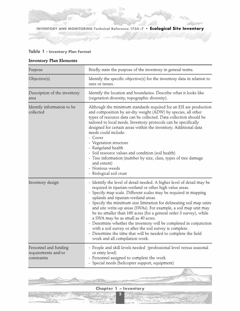
Table 1 - Inventory Plan Format
Inventory Plan Elements
Purpose Briefly state the purpose of the inventory in general terms.
Objective(s) Identify the specific objective(s) for the inventory data in relation touses or issues.
Description of the inventory Identify the location and boundaries. Describe what it looks like area (vegetation diversity, topographic diversity).
Identify information to be Although the minimum standards required for an ESI are productioncollected and composition by air-dry weight (ADW) by species, all other
types of resource data can be collected. Data collection should betailored to local needs. Inventory protocols can be specificallydesigned for certain areas within the inventory. Additional dataneeds could include:- Cover- Vegetation structure- Rangeland health- Soil resource values and condition (soil health)- Tree information (number by size, class, types of tree damage
and extent)- Noxious weeds- Biological soil crust
Inventory design - Identify the level of detail needed. A higher level of detail may berequired in riparian-wetland or other high value areas.
- Specify map scale. Different scales may be required in mappinguplands and riparian-wetland areas.
- Specify the minimum size limitation for delineating soil map unitsand site write-up areas (SWAs). For example, a soil map unit maybe no smaller than 160 acres (for a general order 3 survey), whilea SWA may be as small as 40 acres.
- Determine whether the inventory will be completed in conjunctionwith a soil survey or after the soil survey is complete.
- Determine the time that will be needed to complete the fieldwork and all compilation work.
Personnel and funding - People and skill levels needed (professional level versus seasonal requirements and/or or entry level)constraints - Personnel assigned to complete the work
- Special needs (helicopter support, equipment)

INVENTORY AND MONITORING Technical Reference 1734–7 • Ecological Site Inventory
Chapter 1 – Inventory3
Logistics - Aerial photo or remote sensing needs- Agreements or MOUs- Transportation (vehicles, helicopter)- Office space- Chemical storage space (HCL, pH reagents) - Lodging (camps, motels)- Food or per diem requirements- Equipment, photos, maps (some procurement may be needed 1
year in advance)- Contracts- Administrative support- Coordination with local officials and notification in the local
newspaper, particularly if helicopters are used
Field measurements and - Minimum standards. Production and composition by species, byprocedures SWA, and by ecological site are required.
- Number and size of plots- Other data collection methods to be used (Daubenmire, step
point, line intercept, point frame)- Handbooks and other written guidance- Data collection (forms, field data recorders)
Compilation procedures - Maps- Cartographic requirements- Geographic Information System (GIS) support- Data storage. Method of tabular data input into the Inventory
Data System (IDS) (local entry into Bureau database)- Types of reports to be generated and for whom
Reporting and quality control - Training(inventory reviews and results) - Sampling and harvesting protocolsrequirements - Personnel supervision in the field
- Frequency of progress reports (weekly, monthly)- Who is responsible and when progress and final reports are due
Approval Process - Who the responsible individuals are- When- What the administrative levels are
File Maintenance Identify where the field worksheets, maps, and reports will be storedand plans for computerizing the data. Data must be entered in theBureau’s vegetation database. To determine how it will be entered,contact the National Science and Technology Center (NSTC) in Denver.

INVENTORY AND MONITORING Technical Reference 1734–7 • Ecological Site Inventory
Chapter 1 – Inventory4
Inventory Plan Reviews The inventory plan needs to be reviewed annuallyif the inventory takes longer than 1 year to com-plete. All changes should be documented. Theinventory plan should set forth when and howreviews will be conducted. The inventory teamshould conduct the reviews. Objectives shouldbe reviewed to ensure adequate quality andquantity of inventory progress and to identifyproblems that need management attention.
Inventory TeamThe inventory team generally consists of a teamlead, a soil survey team, a vegetation mappingteam, a vegetation transecting team, and a
phenological data collection team. A soil surveyteam may not be necessary if the survey isalready done. Also, if specified in the inventoryplan, the soil survey and vegetation mappingteams may be combined into a single team tocomplete the mapping of the inventory area.Figure 1, Composition of Inventory Team, isonly a recommendation. Composition of theactual teams will be decided by each individualfield office.
Inventory team members must be selected care-fully. The combined knowledge, experience, edu-cation, and training of each member is extremelyimportant. All specialists on the inventory teamwill need to work closely together throughoutthe inventory.
Figure 1 - Composition of Inventory Team
Ecological Site Inventory Team Organization
Soil SurveyTeam
VegetationMapping
Team
VegetationTransecting
Team
Phenological DataCollection Team
TeamLead

INVENTORY AND MONITORING Technical Reference 1734–7 • Ecological Site Inventory
Chapter 1 – Inventory5
Team LeadThe team lead should be a BLM permanentemployee with supervisory experience. Leadsshould be selected for their knowledge, experi-ence, competence, and good judgment. Theyshould be knowledgeable and experienced in theobjectives and procedures of ecological siteinventories and acquainted with the Bureau’sinterrelated programs. They are responsible fororganizing and directing the inventory, coordi-nating field data collection, assigning work,keeping equipment in good operating order,administrative support (time sheets, leaveapproval, employee evaluations, travel, training)and reporting the progress of the inventory.
Soil Survey TeamThe soil survey team is needed only if a soil sur-vey has not been completed or if the existingsurvey needs further refinement. The team mayinclude employees from BLM, NRCS, combinedBLM-NRCS, or contract personnel.
Vegetation Mapping TeamThe vegetation mapping team usually works inclose contact with the soil survey team and isresponsible for the delineation of ecological sites,successional status, and present vegetation com-munities. Team members should include anexperienced vegetation management specialist(e.g., rangeland management specialist, forester,ecologist, botanist), a soil scientist, and a wildlifebiologist. If riparian-wetland sites are involved inthe inventory, a hydrologist is critical, at leastduring the planning, soil survey, and vegetationmapping phases. These specialists must befamiliar with the soils and plant and animalcommunities of the inventory area.
Vegetation Transecting TeamThe vegetation transecting team is usuallycomprised of rangeland management specialists,
biologists, botanists, and foresters. A knowledgeof the plants in the inventory area is required,along with a good plant taxonomy background.Botany expertise may be required full or parttime. For riparian-wetland inventory updates, atleast one vegetation specialist with experience inwetland ecology and wetland plant taxonomy isneeded.
Phenological Data Collection TeamIt may be desirable to assign the responsibility ofcollecting data for phenological adjustment fac-tors to one or two individuals. This will ensureaccurate data collection in a timely manner forthis important phase of the inventory. This teammay also collect samples for air-dry weight(ADW) conversion data.
Natural Resource Specialists on theInventory TeamThe following natural resource specialists canprovide the necessary experience and expertiseas part of the individual teams that form themain inventory team.
Soil ScientistThe soil scientist is responsible for mappingecological sites and developing soil map units.
Vegetation Management SpecialistThe vegetation management specialist isresponsible for mapping vegetation communi-ties and administrative boundaries; collectingvegetation and related resource data (e.g.,production, cover, rangeland health, structure);and assisting the soil scientist in mappingecological sites and developing soil map units.
The vegetation management specialist can bea botanist, biologist, rangeland managementspecialist, forester, or anyone proficient inidentifying vegetation species. This expertise is
INVENTORY AND MONITORING Technical Reference 1734–7 • Ecological Site Inventory
Chapter 1 – Inventory6
usually involved to some degree on all phasesof the inventory (i.e., vegetation mapping, soilsurvey, transecting, and phenology) includinginventory plan preparation.
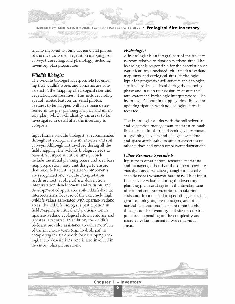
Wildlife BiologistThe wildlife biologist is responsible for ensur-ing that wildlife issues and concerns are con-sidered in the mapping of ecological sites andvegetation communities. This includes notingspecial habitat features on aerial photos.Features to be mapped will have been deter-mined in the pre- planning analysis and inven-tory plan, which will identify the areas to beinvestigated in detail after the inventory iscomplete.
Input from a wildlife biologist is recommendedthroughout ecological site inventories and soilsurveys. Although not involved during all thefield mapping, the wildlife biologist needs tohave direct input at critical times, whichinclude the initial planning phase and area basemap preparation; map unit design to ensurethat wildlife habitat vegetation componentsare recognized and wildlife interpretationneeds are met; ecological site descriptioninterpretation development and revision; anddevelopment of applicable soil-wildlife-habitatinterpretations. Because of the extremely highwildlife values associated with riparian-wetlandareas, the wildlife biologist’s participation infield mapping is critical and participation inriparian-wetland ecological site inventories andupdates is required. In addition, the wildlifebiologist provides assistance to other membersof the inventory team (e.g., hydrologist) incompleting the field work for developing eco-logical site descriptions, and is also involved ininventory plan preparations.
HydrologistA hydrologist is an integral part of the invento-ry team relative to riparian-wetland sites. Thehydrologist is responsible for the description ofwater features associated with riparian-wetlandmap units and ecological sites. Hydrologicinput for progressive soil surveys and ecologicalsite inventories is critical during the planningphase and in map unit design to ensure accu-rate watershed hydrologic interpretations. Thehydrologist’s input in mapping, describing, andupdating riparian-wetland ecological sites isrequired.
The hydrologist works with the soil scientistand vegetation management specialist to estab-lish interrelationships and ecological responsesto hydrologic events and changes over timeand space attributable to stream dynamics orother surface and near-surface water fluctuations.
Other Resource SpecialistsInput from other natural resource specialistsand managers, other than those mentioned pre-viously, should be actively sought to identifyspecific needs whenever necessary. Their inputis especially valuable during the inventoryplanning phase and again in the developmentof site and soil interpretations. In addition,assistance from recreation specialists, geologists,geomorphologists, fire managers, and othernatural resource specialists are often helpfulthroughout the inventory and site descriptionprocesses depending on the complexity andresource values associated with individualareas.

INVENTORY AND MONITORING Technical Reference 1734–7 • Ecological Site Inventory
Chapter 1 – Inventory7
Preparing for Field OperationsThe team lead formulates a plan of operation,assembles materials and equipment, makesnecessary arrangements, and coordinates withappropriate field office staff. The lead is respon-sible for ensuring that all forms, maps, photos,and other equipment and supplies necessary forconducting the inventory are available.
Training and OrientationThe training and orientation of the inventoryteam is the responsibility of the team lead. Thelead is responsible for assessing specific trainingneeds. This includes scheduling and preparingtraining in procedures (e.g., mapping units, datacollection, plant identification, aerial photo inter-pretation). It also includes orientation to the geo-graphical inventory area and rangeland users.
It is particularly important that the inventoryteam be well trained on measurement tech-niques. The inventory team should have a basicunderstanding of the kinds and amount of dataneeded and the intended uses of the data.
The need for training in specific sampling tech-niques for each discipline represented in an eco-logical site inventory will vary greatly dependingon individual background and expertise.
The following are recommended courses:
• Inventory and Monitoring of Plant Populations(BLM National Training Center (NTC) Course1730-05). Presents information on inventory,monitoring, analysis, and evaluation tech-niques for vegetation and plant populations.
• The Ecological Site Concept (BLM NTCCourse 4000-ST-2, self-study course andvideo). Provides basic instruction on soil mapunits, ecological site concepts, and SWA map-ping criteria.
• Coordinated Riparian Area Management (BLMNTC Course 1737-1). Provides an introductionto riparian-wetland ecological site concepts, aswell as substantial information on BLM ripari-an-wetland policies, values, and managementconcepts.
• Riparian-Wetland Ecological Site Classification(BLM NTC Course 1737-4). Advanced coursefor mapping and describing riparian-wetlandsites.
• GIS - Geodata for Resource Specialists (BLMNTC Course 1730-11). Provides a basic under-standing and hands-on experience in the con-cepts, use, and application of GIS.
• Basic Aerial Phot Interpretation (BLM NTCCourse 9160-1). Provides students with thebackground and ability to interpret and usevarious kinds of aerial photography.
• Soils - Basic Soil Survey: Field and Laboratory(NRCS National Employee DevelopmentCenter (NEDC), Fort Worth). Designed to pro-vide new soil scientists and other specialists anopportunity to experience what it takes tocomplete a soil survey. Output potential of soilinterpretations and use of field and laboratorymethods and data analysis in soil survey arealso discussed.
INVENTORY AND MONITORING Technical Reference 1734–7 • Ecological Site Inventory
Chapter 1 – Inventory8
Additional courses recommended for specificdisciplines include:
• ECS - Range Plant Ecology (NRCS NEDC, FortWorth). Advanced course that provides infor-mation on the ecological interaction of rangevegetation.
• RES CONS - Saline and Sodic Soils (NRCSNEDC, Fort Worth). Provides a backgroundand hands-on experience in understandingchemical relationships, testing and analyzingdata, recognizing problems, and recommendingmanagement solutions.
• Soils - Soil Correlation (NRCS NEDC, FortWorth). Advanced course for soil scientistsprovides insight and techniques to apply soilclassification, soil correlation procedure, geo-morphic relationships, soil survey area hand-book development, and laboratory data analysisand sampling procedures.
• Soils - Soil Lab Data Use (NRCS NEDC, FortWorth). Advanced course for soil scientistsprovides insight and techniques for using labo-ratory data in soil classification and plantrelationships.
• Soils - National Soil Information System(NASIS) (NRCS). Advanced course for soil sci-entists familiarizes students with NASIS struc-ture, spreadsheet organization, and how topopulate NASIS data fields.
Aerial Photographs and MapsAerial photographs and maps are important toolsin the inventory process. They help identifylocations of natural landscape and special features
and assist in mapping soils, vegetation communi-ties, and special habitat features.
Aerial PhotographsIt is essential to have a complete set of aerialphotographs for inventory purposes. Theseshould be acquired well in advance of the inven-tory. To facilitate the inventory, more recent (lessthan 10 years old) photos are the most desirable.Natural color or color-infrared photography isbest for mapping vegetation, and a scale of1:24,000 is best suited for ease of transferring theinformation to orthophoto quads or topographicmaps. The aerial photos or orthophoto quads areused for field mapping and this information isthen transferred to the map base. Aerial photosare helpful in seeing greater detail, but orthophotosare better for mapping. Refer to Appendix 1 fordetails on acquiring aerial photos.
Orthophoto QuadsOrthophoto quads are distortion-free imagemaps at 1:24,000 scale. They are excellent toolsfor mapping data in the field or from aerialphotography. They can also be scanned andgeoreferenced for inclusion in GIS. With anortho image as a backdrop, the user can digitizethe inventory units, display global positioningsystem (GPS) data, or analyze other data layers.Also available in most areas are Digital OrthoQuarter Quads (DOQQ), which have replacedpaper and film orthophotos and are GIS-readyimages. Contact your State Office GIS coordinatorabout availability.
Topographic and Planimetric MapsUse topographic and planimetric maps or anyhigh-quality maps that accurately show therelative position and nature of the inventoryarea features. U.S. Geological Survey (USGS)topographic quadrangles at 1:24,000 scale are the
INVENTORY AND MONITORING Technical Reference 1734–7 • Ecological Site Inventory
Chapter 1 – Inventory9
most useable and available. They, too, come indigital format for GIS and are called USGSDigital Raster Graphics (DRG).
Administrative MapsAdministrative maps include information such asmanagement units or grazing allotment bound-aries, range improvements, timber harvests, fishand wildlife habitat, and land status. They areuseful references for team members during theinventory and can be integrated as data layers foranalysis in GIS if they have been digitized.Overlays can be made for use with orthophotoquads as well.
Other MapsTopographic maps overlaid with geology, pre-cipitation, and land ownership are helpful inmapping soils and ecological sites.
Remote Sensing ImageryRemote sensing images may be helpful in map-ping landscape features, vegetation communities,and soils. Remote sensing images can beobtained at comparable scales to orthophotoquads providing multispectral information.
General EquipmentEquipment and tools include items such as pho-tos, maps, references, forms, pens, pencils,Quadrat frames, and balance scales. Table 2 listsgeneral equipment common to each discipline.

INVENTORY AND MONITORING Technical Reference 1734–7 • Ecological Site Inventory
Chapter 1 – Inventory10
Table 2 - Equipment List
General Equipment Soils Vegetation Wildlife HydrologyBiology
Inventory plan x x x xMemorandum of Understanding (MOU) x x x xManuals and handbooks
(see specific lists under Soil, etc.) x x x xForms x x x xField notebook x x x xExisting site descriptions common to the
inventory area x x x xPlant ID references x x xList of plant names and symbols found
in the State x x xGeomorphology reports for the area
and related scientific papers xPlat or land status maps x x x xAbney level or clinometer x x xStereoscope (mirror and pocket) x xCamera x x x xPens and pencils x x x xCompass (magnetic) x xQuadrat frames xPin flags xPaper bags xBalance scales xClippers and grass sheers xRubber bands xAuger or probe (hand and/or power) x x xShovel (standard) and tile spade x x xTape measure (metric and English) x x x xComputer x x x xVehicle and aircraft x x x xFirst aid kit x x x x
INVENTORY AND MONITORING Technical Reference 1734–7 • Ecological Site Inventory
Chapter 1 – Inventory11
Specialized EquipmentThe following information lists additional equip-ment and references specific to each discipline.
SoilsSpecific soils needs include, but are not limitedto:
• Manuals and handbooks on procedural guidanceand other references- NRCS National Soil Survey Handbook
(430-VI-NSSH, 1996)- Soil Survey Manual (Agriculture Handbook
No. 18, Oct 1983)- Soil Taxonomy (2nd edition Agriculture
Handbook No. 436 and recent amendments)- SMSS Keys to Soil Taxonomy (8th Edition,
1998)- NRCS National Range and Pasture
Handbook (NRPH)- NRCS National Forestry Manual (NFM)- NRCS National Biology Manual (NBM)- NRCS National Cartographic Manual (NCM)- NRCS Field Handbook for Describing and
Sampling Soils- USDA-NRCS Soil Series of the United States
(www.statlab.iastate.edu/soils)- State Hydric Soil List- For other suggested technical references, see
Section 602-4 of the National SoilsHandbook (NSH).
• Forms - NRCS Field Indicators of Hydric Soils in the
United States (Version 4.0, March 1998)- Map Unit Transect forms commonly used in
the State NRCS-SOI-232 Pedon Descriptionor as revised by the State
- NRCS-SOI-232F Soil Description or otherlike forms commonly used in field note taking
- Access to the soil survey database softwarefor data entry into NASIS forms and retrieval
• Field Soil Survey Database (FSSD) for transectmanagement, pedon management, map unitrecords (NASIS), soils database software
• Pedon description program software
• EquipmentAltimeterBackhoe (mounted on 1-ton truck)Color charts (Munsell)Digging barElectric conductivity meterGeology pickGlobal positions system unitHand lensHydrochloric acid (10% solution) KnifeLight tableMap boardpH kit (chemical)pH meterSieve setSoil analysis (portable field laboratory)Soil sample bags and boxesSoil hand augerSoil test kit (chemical)Soil thermometerSpot plateWater bottles
VegetationSpecific vegetation needs include, but are notlimited to:
• Manuals and handbooks on procedural guidanceand other references- NRCS National Range and Pasture
Handbook (NRPH)

INVENTORY AND MONITORING Technical Reference 1734–7 • Ecological Site Inventory
Chapter 1 – Inventory12
- BLM Manual 4400 Rangeland Inventory,Monitoring, and Evaluation
- BLM Manual 1737-7 Procedures forEcological Site Inventory–With SpecialReference to Riparian-Wetland Sites
- National List of Plant Species That Occur inWetlands (USFWS)
- Soil-site correlation legend- Soil map unit descriptions
• Forms- Vegetation Production Worksheet (Appendix 4)- NRCS Range 417 or equivalent form
• IDSU (Inventory Data System Utilities) com-puter program and/or access to IDS at NSTC
• Equipment - Rope (plots 96 ft2, 0.01 acre, .01 acre) - Planimeters (if acreages are to be compiled
by field crews)
Wildlife BiologySpecific wildlife biology needs include, but arenot limited to:
• Manuals and handbooks on procedural guidanceand other references - BLM Manual 6602, Integrated Habitat
Inventory and Classification System (IHICS)- Reference guides for the identification of
birds, mammals, and reptiles
• Forms- Animal Species Occurrence 6602-1- Special Habitat Features 6602-2- Resource Field Data Sheets 6602-3
• Computer software and documentation- Integrated Habitat Inventory and
Classification System (IHICS)
- Special Status Species Tracking (SSST)- Species Tracking System (STS)
• Equipment- Field glass- Magnifying glass
HydrologySpecific hydrology needs include, but are notlimited to:
• Manuals and handbooks on procedural guidanceand other references- Stream Classification Reference (Rosgen,
unpublished)- Water Resources Council Bulletin #17B of
the Hydrology Committee, “Guidelines forDetermining Floodflow Frequency”
- USGS Techniques of Water-ResourceInvestigations Reports:
Book 3, Chapter A1: General field andoffice procedures for indirect dischargemeasurementsBook 3, Chapter A2: Measurement of peakdischarge by the slope-area methodBook 3, Chapter A8: Discharge measure-ment at gaging stationsBook 4, Chapter A2: Frequency curvesBook 4, Chapter B1: Low-flow investigations
- Reference guide for estimating Manning'sroughness coefficient
- Reference guides for water-quality fieldtechniques
• Computer Software and Documentation- Statistical software, with documentation,
capable of performing frequency analysisusing a log-Pearson Type III frequencydistribution

INVENTORY AND MONITORING Technical Reference 1734–7 • Ecological Site Inventory
Chapter 1 – Inventory13
- Open-channel flow software, with documen-tation, capable of analyzing channel cross-section data, using normal depth and/or stan-dard step calculations to produce relation-ships between discharge and other hydraulicparameters
• Equipment- Surveying equipment
Level, rod, tripod, and survey notebook- Discharge measuring equipment
Top-setting wading rodCurrent meter (Marsh-McBirney orvertical-axis current meter)Headset and stopwatch (if using vertical-axis current meter)ClipboardUSGS discharge measurement forms
- Well points- Water quality sampling equipment
ThermometerConductivity meter and calibration standardspH meter and calibration standardsBottles, labels, and preservatives for watersamplesCoolers with ice for sample transport tolaboratoryField formsSampling equipment for special situations
Depth-integrating sampler (e.g., DH-48),treated for trace elements, for integratedcross-section samplingBedload or bed-material samplingequipmentSubmersible, peristaltic, or other pumpfor shallow ground-water samplingField filtration equipment for samplingdissolved chemical constituents, asopposed to sampling for total chemistry

S
INVENTORY AND MONITORING Technical Reference 1734–7 • Ecological Site Inventory
Chapter 2 – Soils15
Chapter 2 - SoilsSoil Map UnitSOIL SURVEY INFORMATION IS IMPORTANTin mapping ecological sites and vegetation com-munities. One major feature of a soil survey isthe soil map unit–a group of soil areas or miscel-laneous areas delineated in a soil survey. Smallareas of similar and dissimilar soils are classifiedas inclusions. Inclusions are discussed in the soilsurvey map unit description, but are not mappedbecause they are either too small to be delineatedat the scale of mapping or their interpretationsare similar to the dominant soil.
There are four kinds of soil map units: consocia-tion, complex, association, and undifferentiatedgroup. (See the National Soils Handbook (NSH),pages 627-10 and 11). The consociation map unitis the most easily understood level of mappingbecause only one ecological site is delineated,although mapping at such a fine detail level maynot be practical due to minimum size delineations.
ConsociationA consociation is a map unit where the dominantsingle soil taxon or miscellaneous area makes upat least 50 percent of the area.
In a consociation, the similar soils or miscellaneousareas (soils or miscellaneous areas so similar tothe dominant component that major interpreta-tions do not significantly differ) make up lessthan 50 percent of the unit.
The total amount of dissimilar inclusions (soilswhose interpretations differ from the dominantsoil) generally does not exceed about 15 percent
if the minor components are limiting (soilswhose interpretations limit the use of the soilmore than the dominant soil) and 25 percent ifthey are nonlimiting.
ComplexA complex is a collection of two or more dis-similar kinds of soils or miscellaneous areas in aregular repeating pattern so intricate that theycannot be delineated separately due to the scaleof mapping selected.
A complex consists of two or more of the fol-lowing: different soils series, and/or differentphases of soils series, and/or miscellaneous areasthat occur in regular patterns like rock outcrops.
The total amount of dissimilar inclusions (soilswhose interpretations differ from the dominantsoil) generally does not exceed about 15 percentif the minor components are limiting (soilswhose interpretations limit the use of the soilmore than the dominant soil) and 25 percent ifthey are nonlimiting.
AssociationAn association is similar to a complex, but differsbecause the major soil components or miscella-neous areas occur in repeatable patterns andcould have been broken out into separate soilmap units at the scale of mapping but were not.

INVENTORY AND MONITORING Technical Reference 1734–7 • Ecological Site Inventory
Chapter 2 – Soils16
Soil association maps for low intensity land usemanagement are more efficient and cost effectivethan more detailed mapping without detractingfrom the utility of the soil survey. It is more effi-cient to group and interpret several soils into onemap unit rather than delineate separate mapunits.
The information about individual soil series arenot lost, since their percentages and positions onthe landscape are identified in the soil map unitdescription.
The total amount of dissimilar inclusions (soilswhose interpretations differ from the dominantsoil) generally does not exceed about 15 percentif the minor components are limiting (soilswhose interpretations limit the use of the soilmore than the dominant soil) and 25 percent ifthey are nonlimiting.
Undifferentiated GroupUndifferentiated soil groups consist of two ormore taxon components that are not consistentlyassociated geographically and therefore do notalways occur together in the same map unit.These taxa are included in the same named mapunit because use and management of the soilsare the same or are very similar for common uses.
Every delineation in an undifferentiated grouphas at least one of the major components andmay have all the components.
The same principles regarding the proportion ofminor components that apply to consociationsalso apply to undifferentiated groups
Soil Map Unit DevelopmentSoil map units are developed based on broadlandscape features. These landscape features arefurther broken down into characteristic land-forms and geomorphic components, such ashills, side slopes, toe slopes, floodplains, anddepressions. The kinds of areas associated withthese segments are then identified. Often, dis-tinct vegetation patterns occur along these samelandform and geomorphic surfaces. Generally,soil map units represent soil components that arerepeated on the landscape.
Soil Map Unit DescriptionsSoil map unit descriptions characterize the mapunit as it is identified and delineated during thesoil mapping process. The contents of a map unitdescription will provide information to the userdetailing the setting for each dominant soil com-ponent. A brief soil profile description is giventhat details distinctive surface features, vegeta-tion relationships, and soil properties that affectuse and management. All dissimilar soil inclu-sions are identified and their differences in land-scape setting and soil profile characteristics arenoted in the description. From these descriptions,the user should be able to determine the patternsand percent of occurrence of each componentsoil and soil inclusion within the map unit andtheir position on the landscape.
Detailed Soil MapsBase maps of soil surveys are primarily oftwo kinds:
• Rectified photo base maps (high-altitudephotography)

INVENTORY AND MONITORING Technical Reference 1734–7 • Ecological Site Inventory
Chapter 2 – Soils17
• Orthophoto base maps (high-altitude photographywith the displacement of images removed).
Soil map units are delineated on the base map toprovide location and spatial relationships of soilsfor subsequent analysis. A map unit symbol caneither be numeric, alphabetic, or a combinationof both (NSH, page 627-7). It consists of no morethan five elements (characters), including digits,letters, and hyphens that identify the delineation.The best way to assign map unit symbols is tosequentially number them and add alpha charac-ters to describe the slope range of the map unit.The symbol also provides the reference to a mapunit description and associated information. It’spossible that field map unit symbols couldchange at final correlation prior to the publicationof the soil survey.
Soil Survey Mapping for Riparian-Wetland AreasMost published soil survey maps, especially atthe 1:24,000 scale are not detailed enough todelineate riparian-wetland areas, most streams,seeps, springs, potholes, and other small wetareas. This may necessitate delineating soil mapunits on a larger scale photo.
One alternative, where GIS capability is available,is to photographically or digitally enlarge anorthophoto quad base map to scales between1:6,000 and 1:12,000 (Batson et al., 1987), delin-eate and identify the riparian-wetland map units,and then digitize the areas of the base maps. It isfeasible to map riparian-wetland areas at a photoscale of 1:2,400 and perform a map transfer to1:6,000 scale (a reduction of 2.5 times) if thatamount of detail is needed. Riparian- wetland mapunit delineations using this method would be quitesmall, but data entry into GIS would be possible.
A second alternative is to simply designate linesegments on a scale of 1:24,000 to representstream segments as a map unit and spot symbolmap units for other kinds of riparian-wetlandareas. When either line-break to line-break ordot-to-dot line segments and ad hoc or dot spotsymbols are used, the average width of streamsegments or the average area of spot symbols willhave to be described in the map unit description.This method is used with or without GIS capa-bility and soil survey area base maps are neededfor reports. See Appendix 2, Soil Map UnitDelineations, for more details on using thesetechniques. Figure 2 is a schematic representationof a soil map that includes line segments. Eacharea with a symbol represents a soil map unit.
676 15801490
174
175
681
585
173
174
123
123
123
252
251
252
1230
1230
1230
1580
Figure 2 - Schematic Representation of SoilMap with Line Segments. Each area with asymbol represents a soil map unit.
INVENTORY AND MONITORING Technical Reference 1734–7 • Ecological Site Inventory
Chapter 2 – Soils18
Importance of Soil Map UnitsThe soil map unit provides the spatial relation-ship between soils or groups of soils and land-scapes. The map unit also provides the linkbetween the location of named soil taxa and tab-ular information on specific soil properties andinterpretations for use and management.
In addition, soil map unit delineations providethe initial spatial relationship between ecologicalsites, which are correlated to the soil compo-nents of a map unit. Because of the relationshipbetween landscape patterns, soils, and ecologicalsites, soil maps are an excellent base for otherresource delineations or interpretive maps, suchas wildlife habitat, recreational areas, watershedconditions, livestock utilization, and many others.

R
INVENTORY AND MONITORING Technical Reference 1734–7 • Ecological Site Inventory
Chapter 3 – Ecological Sites19
Definition of Ecological SiteRANGELAND LANDSCAPES ARE DIVIDEDinto ecological sites for the purposes of inventory,evaluation, and management. An ecological siteis a distinctive kind of land with specific physicalcharacteristics that differs from other kinds ofland in its ability to produce a distinctive kind andamount of vegetation. It is the product of all theenvironmental factors responsible for its devel-opment, and it has a set of key characteristics(soils, hydrology, and vegetation) that are includedin the ecological site description. Developmentof the soils, hydrology, and vegetation are allinterrelated. Each is influenced by the other andinfluences the development of the others.
An ecological site has characteristic soils thathave developed over time throughout the soildevelopment process. The factors of soil devel-opment are parent material, climate, livingorganisms, topography or landscape position,and time. These factors lead to soil developmentor degradation through the processes of loss,addition, translocation, and transformation. Soilswith like properties produce and support a dis-tinctive kind and amount of vegetation and aregrouped into the same ecological site.
An ecological site has a characteristic hydrology,particularly infiltration and runoff, that hasdeveloped over time. The development of thehydrology is influenced by development of thesoil and plant community.
An ecological site has evolved a characteristickind (cool season, warm season, grassland,shrub-grass, sedge meadowland) and amount ofvegetation. The plant community on an ecological
site is typified by an association of species thatdiffers from that of other ecological sites in thekind and/or proportion of species or in annualproduction. These vegetation communitiesevolved with a characteristic kind of herbivory(kinds and numbers of herbivores, seasons ofuse, intensity of use) and fire regime. Fire fre-quency and intensity contributed to thecharacteristic plant community of the site.
Succession and RetrogressionSuccession is the process of soil and plantcommunity development on an ecological site.Retrogression is the change in species compositionaway from the historic climax plant communitydue to management or severe natural climaticevents.
Succession occurs over time and is a result ofinteractions of climate, soil development, plantgrowth, and natural disturbances existing on thesite through time. Primary succession is the for-mation process that begins on substrates havingnever previously supported any vegetation (e.g.,lava flows, volcanic ash deposits). Secondarysuccession occurs on previously formed soil fromwhich the vegetation has been partially orcompletely removed.
Ecological site development associated withclimatic conditions and normal range of distur-bances (e.g., occurrence of fire, grazing, unusuallywet periods, flooding) produce a plant communityin dynamic equilibrium with these conditions.This plant community is referred to as the historicclimax plant community.
Chapter 3 - Ecological Sites
INVENTORY AND MONITORING Technical Reference 1734–7 • Ecological Site Inventory
Chapter 3 – Ecological Sites20
Vegetation dynamics on an ecological siteincludes succession and retrogression. Thepathway of secondary succession is often notsimply a reversal of disturbances responsible forretrogression and may not follow the samepathway as primary succession.
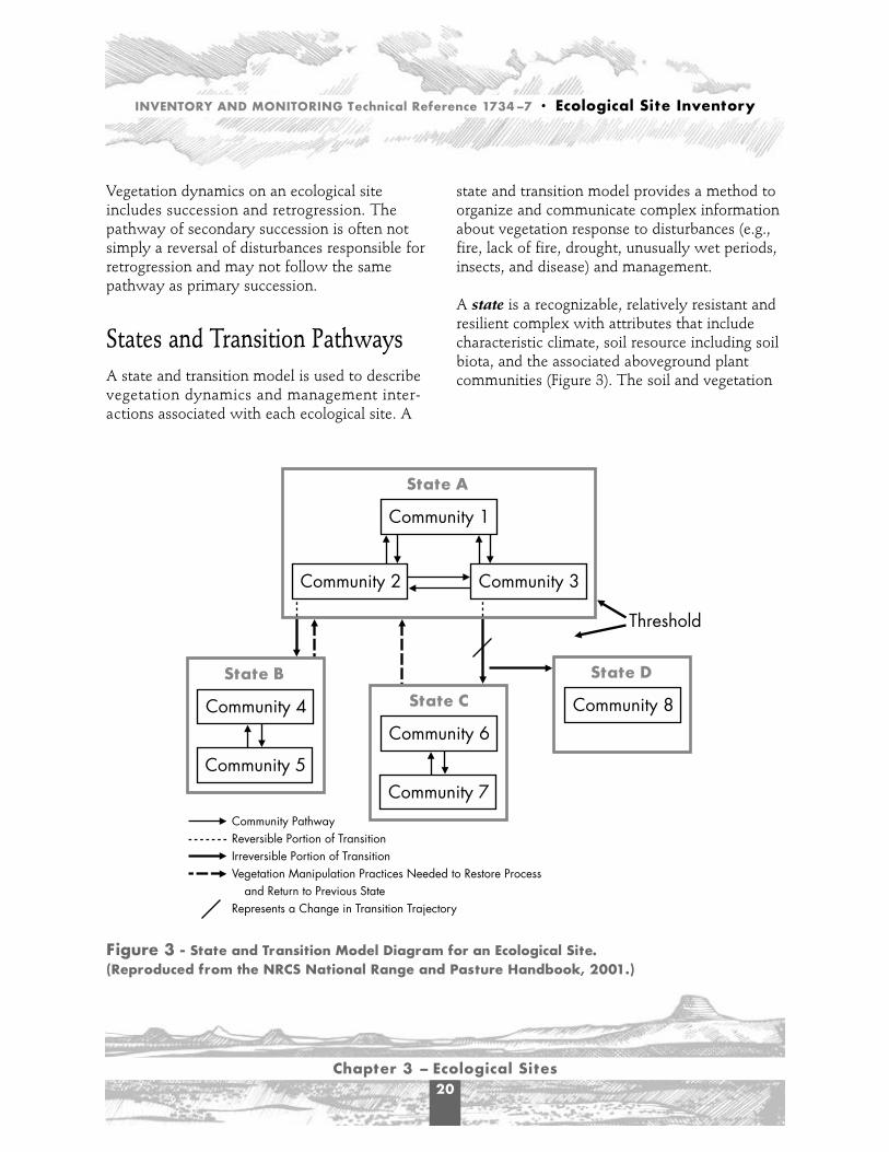
States and Transition PathwaysA state and transition model is used to describevegetation dynamics and management inter-actions associated with each ecological site. A
state and transition model provides a method toorganize and communicate complex informationabout vegetation response to disturbances (e.g.,fire, lack of fire, drought, unusually wet periods,insects, and disease) and management.
A state is a recognizable, relatively resistant andresilient complex with attributes that includecharacteristic climate, soil resource including soilbiota, and the associated aboveground plantcommunities (Figure 3). The soil and vegetation
State A
Community 1
Community 2 Community 3
Threshold
State C
Community 6
Community 7
State D
Community 8
State B
Community 4
Community PathwayReversible Portion of TransitionIrreversible Portion of TransitionVegetation Manipulation Practices Needed to Restore Process and Return to Previous StateRepresents a Change in Transition Trajectory
Community 5
Figure 3 - State and Transition Model Diagram for an Ecological Site.(Reproduced from the NRCS National Range and Pasture Handbook, 2001.)

INVENTORY AND MONITORING Technical Reference 1734–7 • Ecological Site Inventory
Chapter 3 – Ecological Sites21
components are inseparably connected throughecological processes that interact to produce asustained equilibrium that is expressed by a spe-cific suite of plant communities. The primaryecological processes are water cycle, nutrientcycle, and the process of energy capture. Eachstate has distinctive characteristics, benefits, andvalues depending upon the intended use, products,and environmental effects desired from the site.
Two important attributes of a state are resistanceand resilience. Resistance refers to the capabilityof the state to absorb disturbance and stressesand retain its ecological structure. Resiliencerefers to the amount of disturbance or stress astate can endure and still regain its original func-tion after the disturbances and stresses areremoved.
States are relatively stable and resistant to distur-bances up to a threshold point. A threshold isthe boundary between two states, such that oneor more of the ecological processes has beenirreversibly changed. Irreversible implies thatrestoration cannot be accomplished through nat-ural events or a simple change in management.Active restoration (e.g., root plowing, seeding,chaining, prescribed fire, intensive grazing man-agement) must be accomplished before a returnto a previous state is possible. Additional thresh-olds may occur along the irreversible portion of atransition causing a change in the trajectorytoward another state as illustrated in Figure 3.Once a threshold is crossed, a disequilibriumamong one or more of the primary ecologicalprocesses exists and will be expressed throughchanges in the vegetative community and even-tually the soil resource. A new stable state isformed when the system reestablishes equilibriumamong its primary ecological processes.
A transition is the trajectory of system changebetween states that will not cease before theestablishment of a new state. Transitions can betriggered by natural events, management actions,or both. Some transitions may occur very quicklyand others over a long period of time. Two por-tions of a transition are recognized: reversibleand irreversible. Prior to crossing a threshold, atransition is reversible and represents an oppor-tunity to reverse or arrest the change. Vegetationmanipulation practices, and if needed, facilitatingpractices, are used to reverse the transition. Oncea threshold is crossed, the transition is irreversiblewithout significant inputs of managementresources and energy. Significant inputs are asso-ciated with accelerating practices, such as brushmanagement and range planting.
States are not static as they encompass a certainamount of variation due to climatic events,management actions, or both. Dynamics withina state do not represent a state change since athreshold is not crossed. In order to organizeinformation for management decisionmakingpurposes, it may be desirable at times to describethese different expressions of dynamics withinthe states. These different vegetative assem-blages within states will be referred to as plantcommunities and the change between thesecommunities as community pathways.
Figure 3 illustrates the different components of astate and transition model diagram for an ecolog-ical site. States are represented by the largeboxes and are bordered by thresholds. The smallboxes represent plant communities with commu-nity pathways representing the cause of changebetween communities. The entire trajectoryfrom one state to another state is considered atransition (i.e., from State A to State B). The

INVENTORY AND MONITORING Technical Reference 1734–7 • Ecological Site Inventory
Chapter 3 – Ecological Sites22
portion of the transition contained within theboundary of a state is considered reversible witha minimum of input from management. Oncethe transition has crossed the threshold, it is notreversible without substantial input (vegetationmanipulation practices). The arrow returning to aprevious state (State B to State A) will be utilizedto designate types of practices needed. Additionalthresholds occurring along a transition maychange the trajectory of a transition (from StateC to State D).
The first vegetation state described in an ecologi-cal site description is the historic climax plantcommunity or naturalized plant community(Community 1 from Figure 3). From this state, a“road map” to other states has been developed.Each transition will be identified separately anddescribed, incorporating as much informationknown concerning the causes of change, changesin ecological processes, and any known probabil-ities associated with the transitions. Plant com-munities and community pathways within statesmay be described as needed.
Historic Climax Plant CommunityThe historic climax plant community for an eco-logical site is the plant community that existedbefore European immigration and settlement.This plant community was best adapted to theunique combination of environmental factorsassociated with the site. The historic climaxplant community was in dynamic equilibriumwith its environment. It is the plant communitythat was able to avoid displacement by the suiteof disturbances and disturbance patterns (i.e.,magnitude and frequency) that naturallyoccurred within the area occupied by the site.Natural disturbances, such as drought, fire,unusually wet periods, and grazing (e.g., native
fauna and insects) were inherent in the develop-ment and maintenance of these plant communi-ties. The effects of these disturbances are part ofthe range of characteristics of the site that con-tribute to that dynamic equilibrium. Fluctuationsin plant community structure and functioncaused by the effects of these natural disturbancesestablish the boundaries of dynamic equilibrium.They are accounted for as part of the range ofcharacteristics for an ecological site. Some sitesmay have a small range of variation, while othershave a large range. Plant communities that aresubjected to abnormal disturbances and physicalsite deterioration or that are protected from nat-ural influences, such as fire and grazing, for longperiods seldom typify the historic climax plantcommunity.
The historic climax plant community of an eco-logical site is not a precise assemblage of speciesfor which the proportions are the same fromplace to place or from year to year. In all plantcommunities, variability is apparent in produc-tivity and occurrence of individual species.Spatial boundaries of the communities, however,can be recognized by characteristic patterns ofspecies composition and community structure.
Naturalized Plant CommunityEcological site descriptions have been developedfor all identified ecological sites. In some parts ofthe country, however, the historic climax plantcommunity has been destroyed, and it is impos-sible to reconstruct that plant community withany degree of reliability. In these regions, sitedescriptions have been developed using the natu-ralized plant communities for the site. The useof this option for ecological site descriptions islimited to those sites where the historic climaxplant community has been destroyed and cannot

INVENTORY AND MONITORING Technical Reference 1734–7 • Ecological Site Inventory
Chapter 3 – Ecological Sites23
be reconstructed with any degree of reliability.The annual grasslands of California are an exampleof a naturalized plant community.
Potential Natural CommunityA potential natural community (PNC) is definedas the biotic community that would becomeestablished on an ecological site if all successionalsequences were completed without interferenceby people under the present environmental con-ditions. The term “potential natural community”was recommended for use by the RangeInventory Standardization Committee (RISC) inits 1983 report to replace the term “historic climaxplant community.” The RISC report’s rationalewas that PNC recognizes past influences byman, including past use and introduced exoticspecies of animals or plants. Man’s influence isexcluded from the present onward to eliminatethe complexities of management. The conceptsof climax and PNC both refer to a relatively stablecommunity resulting from secondary successionafter disturbance. Although man may or may nothave caused the disturbance, succession to climaxor PNC occurs without further perceptibleinfluences of man’s activity. PNC is the preferredterm because it explicitly recognizes that natural-ized exotic species may persist in the final stageof secondary succession and that succession afterdisturbance does not always reestablish theoriginal vegetation.
Historic Climax Plant CommunityVersus Potential NaturalCommunityIn this document, the term “historic climax plantcommunity” is used in reference to the official
ecological site description. NRCS still requiresthe documentation of a historic climax plantcommunity in the revision or preparation of newsite descriptions. BLM managers and resourcepersonal have the option of using a PNC forevaluation of similarity indices rather than anhistoric climax plant community. In order to usePNC there must be compelling evidence that aparticular species or group of species, notincluded in the historic climax plant community,should be included in more advanced successionalvegetation communities.
Changes in Ecological SitePotentialSevere physical deterioration of an ecological sitecan permanently alter the potential to supportthe original plant community. Examples includepermanently lowering the water table, severesurface drainage caused by gullying, and severesoil erosion. When the ecological site’s potentialhas significantly changed, it is no longer consid-ered the same site. A change to another ecologicalsite is then recognized, and a new site descriptionmay need to be developed on the basis of itsaltered potential.
Some ecological sites have been invaded by orplanted to introduced species. The introducedspecies may become well established or natural-ized to the site. They may dominate the site, orthey may continue to occupy part of the siteeven when secondary succession has restoredthe plant community to near historic climax con-ditions. In these cases of invasion or introductionof nonnative species, a change in ecological site isnot recognized because the edaphic and climaticpotential for the site has not been altered.
INVENTORY AND MONITORING Technical Reference 1734–7 • Ecological Site Inventory
Chapter 3 – Ecological Sites24
Characteristic Vegetation States ofan Ecological SiteWhere possible, the historic climax plantcommunity for each ecological site has beendetermined. Where it is not possible to deter-mine the historic climax plant community, thenaturalized plant community will be described.In addition to the historic climax plant commu-nity or naturalized plant community, other plantcommunities that comprise the known steadystates of vegetation will be determined andincluded in future ecological site descriptions.
The description of each plant community shouldhave been considered as an approximation sub-ject to modification as additional knowledgebecomes available.
Characteristics of a plant community obtainedfrom several sources or sites should have beenused to describe the plant communities. The fol-lowing factors have been considered in evaluatingplant information:
• Effects of fire or lack of fire• Impacts of grazing or lack of grazing• Impacts of rodent concentrations• Impacts from insects• Soil erosion or deposition by wind or water• Drought or unusually wet years• Variations in hydrology and storm events• Plant disease• Introduced plant species
The NRCS’ Ecological Site Information System(ESIS) can provide useful data in identifying plantcommunities. This system can be found on theWorld Wide Web at http://plants.usda.gov/esis.
Differentiation BetweenEcological SitesThe following guidelines are used todifferentiate one ecological site from another:
• Significant differences in the species or speciesgroups that are in the historic climax plantcommunity, such as the presence (or absence)of one or more species that make up 10 per-cent or more of the historic climax plantcommunity by air-dry weight (ADW)
• Significant differences in the relative propor-tion of species or species groups in the historicclimax plant community, such as a 20 percent(absolute) change in composition by ADWbetween any two species in the historic climaxplant community
• Significant differences in the total annual pro-duction in the historic climax plant community
• Soil factor differences that determine plantproduction and composition, the hydrology ofthe site, and the functioning of the ecologicalprocesses of the water cycle, nutrient cycles,and energy flow
Any differences in these guidelines (either singlyor in combination) great enough to indicate adifferent use potential or to require differentmanagement, are the basis for establishing ordifferentiating a site.
These guidelines are not definitive for site differen-tiation or combination. The differences betweensites may be finer or broader than the guidelines.Rationale, and the site features listed in therespective ecological site descriptions, shouldreadily and consistently distinguish the differences.

INVENTORY AND MONITORING Technical Reference 1734–7 • Ecological Site Inventory
Chapter 3 – Ecological Sites25
Differences in kind, proportion, or production ofspecies are the result of differences in soil, topog-raphy, climate, and other environmental factors.Slight variations in these factors are not criteriafor site differentiation; however, individual envi-ronmental factors are frequently associated withsignificant differences in historic climax plantcommunities. The presence or absence of awater table within the root zone of highly salinesoil in contrast to a nonsaline soil is dramaticallyreflected in plant communities that such soilssupport. Marked changes in soil texture, depth,and topographic position usually result in pro-nounced differences in plant communities, totalproduction, or both. Therefore, such contrastingconditions in the soil characteristics, climate,topography, and other environmental factorsknown to be associated with a specific ecologicalsite can be used as a means of identifying thesite when the historic climax plant community isabsent.
Generally, one species or group of species domi-nate a site. Dominant status does not vary fromyear to year. Because of their stability in thehistoric climax plant community, dominantspecies have often been used to distinguish sitesand to differentiate one site from another.
In evaluating the significance of kinds, proportion,and production of species or species groups thatare dominant in a historic climax plant commu-nity, and given different soil characteristics, therelative proportion of species may indicatewhether one or more ecological sites are involved.For example, in one area the historic climax plantcommunity may consist of 60 percent bigbluestem and 10 percent little bluestem, and inanother area it may consist of 60 percent littlebluestem and 10 percent big bluestem. Thus,two ecological sites are recognized. Even thoughthe production and species are similar, the
proportion’s difference distinguishes them asseparate sites.
The effect of any single environmental factor canvary, depending on the influence of other factors.For example, soil depth is more significant on asite that receives extra water from runoff or in ahigh precipitation zone than on an upland site ina low precipitation area. An additional 2 inchesof annual rainfall may be highly important in asection of the country that has an arid climate,but of minor significance in a humid climate. Adifference in average annual production of 100pounds per acre, ADW, is of minor importanceon ecological sites capable of producing 2,000pounds per acre. This difference, however, ishighly significant on sites capable of producingonly 200 to 300 pounds per acre. Similar varia-tions in degree of significance apply to most fac-tors of the environment. Consequently, in theidentification of an ecological site, considerationwas given to its environment as a whole, as wellas to the individual components.
Where changes in soils, aspect, topography, ormoisture conditions are abrupt, ecological siteboundaries are distinct. Boundaries are broaderand less distinct where plant communitieschange gradually along broad environmental gra-dients of relatively uniform soils and topography.Making distinctions between ecological sitesalong a continuum is difficult. Thus, the need forsite differentiation may not be readily apparentuntil the cumulative impact of soil and climaticdifferences on vegetation is examined over abroad area.
At times, less frequently occurring plants mayincrease on a site or the site may be invaded byplants not formerly found in the historic climaxplant community. The presence or absence ofthese plants may fluctuate greatly because of

INVENTORY AND MONITORING Technical Reference 1734–7 • Ecological Site Inventory
Chapter 3 – Ecological Sites26
differences in microenvironment, weatherconditions, or human actions. Consequently,using them for site identification can be mislead-ing, so they should not be used to differentiatesites. Site differentiation, characterization, anddetermination are based on the plant communitythat develops along with the soils. A study ofseveral locations over several years is needed todifferentiate and characterize a site.
Availability and accessibility to domestic livestockgrazing are not factors in ecological site determi-nation and differentiation. Site differentiation isbased on those soil characteristics, response todisturbance, and environmental factors that havedirect effect on the nature of the historic climaxplant community production.
Revising Ecological SiteDescriptionsAnalysis and interpretation of new informationabout the soil, vegetation, and other onsite envi-ronmental factors may reveal a need to revise orupdate ecological site descriptions. Because thecollection of such information through resourceinventories and monitoring is a continuousprocess, site descriptions may be reviewed peri-odically for needed revision. It is especiallyimportant that site descriptions be reviewedwhen new data on production or response todisturbance become available. Documented pro-duction data, along with related soil, climate,and physiographic data, will be the basis of thesite description revisions or new site descriptions.
Developing New Ecological SiteDescriptionsA new ecological site description should be pre-pared when data analysis or new informationreveals that a different or new ecological siteexists. Generally, enough land area must be iden-tified to be of importance in the management orstudy of the site before a new site will be developed and described. A new ecological sitemay be differentiated from an existing site whensufficient erosion or other action has occurred tosignificantly alter the site's potential.
BLM ProceduresBLM has the capability to develop new sitedescriptions and propose revisions to existingecological site descriptions. However, each newsite description or proposed change must be pre-pared using the procedure identified in Chapter 3of the NRCS National Range and PastureHandbook. All new and proposed revisions mustbe reviewed and approved by the local and StateNRCS offices.
Naming Ecological Sites onRangelandEcological sites have been named to help usersrecognize the kinds of rangeland in their locality.Names of ecological sites are brief and are basedon readily recognized permanent physical featuressuch as the kinds of soil, climate, topography, ora combination of these features. Examples ofecological site names based on these criteria areDeep Sand, Sandy, Sandy Plains, Limestone Hills,
INVENTORY AND MONITORING Technical Reference 1734–7 • Ecological Site Inventory
Chapter 3 – Ecological Sites27
Clay Upland, Saline Lowland, Gravely Outwash,Level Winding Riparian, Pumice Hills, Sub-irrigated, Wet Meadows, Fresh Marsh, and SandySavanna. Some States have chosen to add thedominant species commonly found on the site tothe ecological site name. Examples are AlkaliBottom (Alkali Sacaton), Desert Clay (Shadscale),and Upland Loam (Basin Big Sagebrush).
Ecological sites having similar soils and topogra-phy may exhibit significant differences in theirhistoric climax plant communities because ofclimatic differences. For example, the averageannual precipitation of a clay loam in southernArizona ranges from 12 to 16 inches.Quantitative evaluation indicates that theamount of vegetation produced in areas whereprecipitation is 16 to 19 inches is significantlymore than that produced in areas where precipi-tation is 12 to 16 inches. Thus, two ecologicalsites are recognized and are distinguished by theinclusion of the precipitation zone (PZ) in thename of the sites, as in Clay Loam Ecological Site12-16 PZ and Clay Loam Ecological Site 16-19 PZ.
The limited number of permanent physiographicfeatures or other features used in naming ecolog-ical sites makes repeated use of these termsinevitable. Deep sands, for example, occur inareas of widely divergent climate and supportdifferent natural plant communities. The nameDeep Sand is appropriate for each of these areas,but obviously it is used throughout the countryto designate several ecological sites. Where thisoccurs within a land resource area, the applicableprecipitation zone or other differentiating factorsare to be included as part of the name. Sites thathave the same name, but are in different majorland resource areas, are different sites.
Numbering Ecological SitesThe ecological site number for rangelandsconsists of five parts:
1. The first character designates whether the siteis a rangeland site (R) or a forest site (F). Sincethis identifier is not actually a part of thenumber, it is rarely used.
2. A three-digit number and one-digit letterrepresenting the Major Land Resource Area(MLRA)
3. A single letter representing a Major LandResource Unit (MLRU)
4. A three-digit site number assigned by theState
5. A two-digit letter State postal code
If the MLRA has only two numbers, a zero isinserted in the first space followed by the twonumbers. The first letter (e.g., A, B, C) followingthe MLRA number represents the MLRA subdi-visions. Where no MLRA subdivisions are identi-fied, an X is used in the fourth space to denotethat there is no MLRA subdivision. The fifthspace is reserved for the MLRU letter for Statesthat use the MLRU designation. For those Statesthat do not use the MLRU designation, a Y isinserted. The next three digits represent the indi-vidual ecological site number and are assignedby the State. The final two letters are the State’stwo-letter postal code. An example of anecological site number is: RO41XC313AZ
Ecological sites for MLRAs that extend intoadjoining States would retain the same identifi-cation number including the State designation

INVENTORY AND MONITORING Technical Reference 1734–7 • Ecological Site Inventory
Chapter 3 – Ecological Sites28
for both States. The State postal code attachedwould be the State that first described the site.
Site descriptions will be labeled as “draft” untilthe NRCS’s State range conservationist approvesthe site description.
Correlating Ecological SitesEcological sites should have been correlatedbetween areas, States, and MLRAs on the basisof soils, proportion of species, and annual pro-duction of the potential plant communities. Inthis process, ecological site descriptions arereviewed to ensure consistency in identifyingand describing the same site across State, area,and MLRA boundaries. These reviews includecomparing similar sites to determine whetherthey are in fact different ecological sites.Correlation also involves the review of soilsinformation to ensure the description matchesthe soil properties in the individual soil series.
Only one name should have been given to asingle site that occurs in adjacent States withinthe same MLRA.
Ecological Site DescriptionA description has been prepared for each ecolog-ical site (see an example in Appendix 3). Thedescription identifies the important resources forthe site that are used to identify, evaluate, plan,develop, manage, and monitor rangelands. Thedescription includes the following information,as appropriate:
HeadingAll ecological site descriptions will identify theUSDA and Natural Resources Conservation Service.
Ecological Site NameThe full name of the site should appear on eachpage of the description.
Ecological Site IDThe site number is a 10-digit number that alsoappears on each page of the description.
Major Land Resource AreaIdentifies the major land resource area code andcommon name.
Interstate CorrelationLists the States that have correlated the site.
Physiographic FeaturesDescribes the occurrence of the site on the land-scape. In reference to the historic climax plantcommunity, includes information on whetherthe site typically generates runoff, receivesrunoff from other sites, or receives and generatesrunoff. Physiographic features include:
• Landform• Aspect• Site elevation

INVENTORY AND MONITORING Technical Reference 1734–7 • Ecological Site Inventory
Chapter 3 – Ecological Sites29
• Slope• Water table• Flooding• Ponding• Runoff class
Climatic FeaturesClimatic features include:
• Frost-free period (length and dates)• Freeze-free period (length and dates)• Mean annual precipitation• Monthly moisture and temperature distribution• Location of climate stations
Influencing Water FeaturesIncludes information regarding water featureswhere the plant community is influenced bywater or the water table from a wetland orstream associated with the site. Water featuresinclude the Cowardin wetland classificationsystem and Rosgen stream classification system.
Representative Soil FeaturesThe main soil properties associated with thesite are briefly described. This includes:
• Properties that significantly affect plant, soil,and water relationships, and the site hydrology
• The extent of flow patterns, and the rills andgullies found in the historic climax plantcommunity
• The amount and patterns of pedestaling andterracettes caused by wind or water inherentto the historic climax plant community
• The size and frequency of wind-scoured areas• The susceptibility of the site to compaction• A description of the expected organic layer and
physical and chemical crusts that might bepresent
Representative soil features include:
• Parent materials• Surface texture• Subsurface texture• Surface fragments• Subsurface fragments• Drainage class• Permeability class• Depth• Electrical conductivity• Sodium absorption ratio• Calcium carbonate equivalent• Soil reaction• Available water holding capacity
Ecological Dynamics of the SiteThe general ecological dynamics of the site aredescribed. Included are the expected changesthat are likely to occur because of variations inthe weather and the effects this might have onthe dynamics of the site. Included are assumptionsregarding site development (e.g., fire frequency,native herbivory).
Plant CommunitiesThis section describes:
• Vegetation dynamics of the site• State and transition model diagram• Common states that occur on the site and the

INVENTORY AND MONITORING Technical Reference 1734–7 • Ecological Site Inventory
Chapter 3 – Ecological Sites30
transitions between states. Included are theplant communities and community pathwayswithin each state.
• Ground cover and structure• Annual production• Growth curves• Photos of each state or community
The first plant community to be describedshould be the interpretative community. Thisplant community will be either the historic cli-max plant community or, where applicable, thenaturalized plant community for the site.
Other states and plant communities that mayexist on the site are also described. One or moreplant communities for each state will bedescribed. Included is a narrative describing thedynamics of each state and plant community andthe causes of community pathway changes. Alsodescribed are the thresholds between states, andinformation that will aid in the identification andevaluation of how the ecological processes of thesite are functioning.
Information regarding transitions between statesshould have been included in the plant commu-nity narrative, as well as causes of change andany known probabilities associated with thetransitions.
Species ListA detailed species list will be included for thehistoric climax plant community and each stablestate plant community known to exist on thesite. Each listing should include the major plantspecies (i.e., common name and scientific name)and their normal relative production expressed inpounds ADW (pounds per acre per year) in thetotal plant community. Species should be listed
by life form and group, including pounds peracre allowable for each group.
Plant GroupsEcological site descriptions usually list plantspecies by groups. Plant groups include:
• Cool season tall grasses• Cool season midgrasses• Warm season tall grasses• Warm season midgrasses• Warm season short grasses• Annual grasses• Perennial forbs• Biennial forbs• Annual forbs• Succulent forbs• Leafy forbs• Shrubs• Half-shrubs• Deciduous trees• Evergreen trees• Cacti• Yucca• Yucca-like plants
Other factors used to identify groups include:
• Kind of plant• Structure• Size• Rooting structure• Life cycle• Production• Niche occupied• Photosynthetic pathways
If plant groups are shown, plant groupings willidentify whether individual species within thegroup have a production limitation or whether a

INVENTORY AND MONITORING Technical Reference 1734–7 • Ecological Site Inventory
Chapter 3 – Ecological Sites31
single species can account for the entire groupallowable.
Groups may be subdivided into separate groupsor combined. For instance, two or three groupsof warm season mid-grasses may be describedbecause of different niches occupied and differ-ences in production, structure, elevation, and cli-matic adaptations in the area of the site.
Cover and StructureThe following table (Table 3) is an adaptation ofthe table on ground cover and structure found inAppendix 3. Table 3 has been changed to more
clearly illustrate ground cover and canopy coverlayers (structure) for use by BLM.
Ground cover is the percentage of material, otherthan bare ground, that protects the soil surfacefrom being hit directly by a raindrop. This wouldinclude first contact with plant canopy cover,biological crust, litter, rock fragments, bedrock,and water.
Canopy cover is the percentage of ground coveredby a vertical projection of the outermost perime-ter of the natural spread of foliage of plants.
Structure is the average height and canopy coverof each layer of vegetation.
Table 3 - Cover and Structure
Ground and Canopy Cover
Structure - Height Above the Ground
Not Applicable 6–12 inches 12–24 inches 24–60 inches 180–240 inches%ground %canopy %ground %canopy %ground %canopy %ground %canopy %ground %canopy
cover cover cover cover cover cover cover cover cover cover
Trees
Shrubs
Forbs
Grasses
Litter
Cryptogams
RockFragments
Bare Ground

INVENTORY AND MONITORING Technical Reference 1734–7 • Ecological Site Inventory
Chapter 3 – Ecological Sites32
Biological Soil Crust CommunitiesInformation on biological soil crust communities(e.g., mosses, lichens, cyanobacteria, algae) usu-ally includes only cover data. However, on tun-dra sites where current production can be deter-mined on lichens and mosses, production maybe expressed as total live biomass.
Total Annual ProductionTotal annual production is shown as the medianair-dry production and the fluctuations to beexpected during favorable, normal, and unfavor-able years. In areas where examples of the his-toric climax plant community are not available,the highest production in plant communities forwhich examples are available have been used.
Plant Community Growth CurvesPlant community growth curves are displayedfor each important plant community. Growthcurves indicate the percent of growth by month(Table 4). This includes:
• Number - This number is used only one timein each State. The first 2 digits are the Statepostal code, and the last 4 digits are consecutivenumbers from 001 to 9999.
• Name - This is a brief descriptive name foreach curve.
If plant community growth curves are notavailable, contact the NRCS.
Table 4 - Plant Community Growth Curves
Growth curve number:Growth curve name:Growth curve description:
Jan Feb March April May June July Aug. Sept. Oct. Nov. Dec.
Ecological Site InterpretationsThis section includes the site interpretations forthe use and management of the site. The infor-mation includes:
Animal CommunityThis narrative describes the major wildlifespecies that occupy or use the site. It will include
any major values or problems associated withtheir use of this site and the plant communitiesthat may occur on it. Special status animalspecies, such as threatened and endangeredspecies, and State or local species of concern arediscussed. General descriptions of the use of thissite by livestock and wild horses and burrosshould also be included. Suitability of the sitefor grazing by season and by kind and class of

INVENTORY AND MONITORING Technical Reference 1734–7 • Ecological Site Inventory
Chapter 3 – Ecological Sites33
livestock will be addressed. Included in the dis-cussion is a list of major barriers to wildlife andlivestock use (e.g., water, topography).
Hydrologic FunctionsThis discussion includes effects on the hydrolog-ic functions from shifts to different plant com-munities. There should be a description of thechanges in infiltration and runoff characteristicsexpected due to changes in plant communitiesand soil surface characteristics. Informationabout water budgets for each plant communitycould be included.
Recreational UsesPotential recreational uses that the site can sup-port or that may influence the management ofthe site should be discussed. Included will be alist of special concerns that affect the mainte-nance of the recreational potentials or site condi-tions that may limit its potential. Also listed areplant species that have special aesthetic values,uses, and landscape value.
Wood ProductsIndicates use or potential uses of significantspecies that may influence the management ofthe site.
Other ProductsIndicates the use or potential uses of other prod-ucts produced on the site. These may includelandscape plants, nuts, berries, mushrooms, andbiomass for energy potentials.
Supporting InformationThis narrative involves information about therelationship of this site to other ecological sites.Includes information regarding documentationand references used to develop the ecological sitedescription.
Associated SitesThis is a listing and description of other ecologi-cal sites that are commonly located in conjunc-tion with this site.
Similar SitesIdentifies and describes ecological sites thatresemble or can be confused with the site.
Inventory Data ReferencesIncludes a listing of sample transects or plotssupporting the site description.
State CorrelationIncludes the states that this site has been corre-lated with.
Type LocalityIncludes the location of a typical example of thesite. Indicates township, range, and section orlongitude and latitude of the specific location.
Relationship to Other EstablishedClassification SystemsIncludes a description of how this ecologicalsite description may relate to other establishedclassification systems.
Other ReferencesIncludes other reference information used in sitedevelopment or in understanding the ecologicaldynamics of the site.
Ecological Site Documentation andReferencesEach ecological site description documents thefollowing information about the preparation ofthe original or latest version of the description:

INVENTORY AND MONITORING Technical Reference 1734–7 • Ecological Site Inventory
Chapter 3 – Ecological Sites34
AuthorshipThe original author’s initials and date. Revisionauthor's initials and revision date.
Site ApprovalIncludes signature, title, and date of the Statetechnical specialist who reviewed and approvedthe ecological site description.
Forestland Ecological SitesForestland ecological site descriptions normallycharacterize the mature forest plant communitythat historically occupied the site as well as theother major plant communities that commonlyoccupy the site. An example of a forestland eco-logical site description can be found in the NRCSNational Forestry Manual, part 537, subpart E,exhibit 537-14.
Separating Forested Lands fromRangelands in Areas Where TheyInterfaceRangeland and forested land ecological sites areseparated based on the historic kind of vegeta-tion that occupied the site. Forested land ecologi-cal sites are assigned and described where thishistoric vegetation was dominated by trees.Rangeland ecological sites are assigned whereoverstory tree production was not dominant inthe climax vegetation.

A
INVENTORY AND MONITORING Technical Reference 1734–7 • Ecological Site Inventory
Chapter 4 – Production Data35
Aboveground VegetationProductionALL PRODUCTION AND COMPOSITION datacollected are based on weight measurements.Weight is the most meaningful expression of theproductivity of a plant community or an individualspecies.
Production is determined by measuring theannual aboveground growth of vegetation. Someaboveground growth is used by insects androdents, or it disappears because of weatheringbefore production measurements are made.Therefore, these determinations represent a pro-ductivity index. They are valuable for comparingthe production of different rangeland ecologicalsites, plant species composition, and similarityindex.
Comprehensive interpretation of plant produc-tion and composition requires that data be repre-sentative of all species having measurable pro-duction. Rangeland and other grazing lands maybe used or have potential for use by livestockand wildlife, as recreation areas, as a source ofcertain wood products, for scenic viewing, andfor other soil and water conservation purposes.The value of plant species for domestic livestockoften is not the same as that for wildlife, recre-ation, beautification, and watershed protection.Furthermore, the principles and concepts ofrangeland ecological site, similarity index, andother interpretations are based on the total plantcommunity. Therefore, interpretations of a plant
community are not limited solely to species thathave value for domestic livestock.
The procedures and techniques discussed in thissection relate primarily to rangeland. Most ofthem, however, also apply to grazeable forestand native or naturalized pasture. Changes ormodifications in procedures required for landother than rangeland are described.
Total Annual ProductionThe total aboveground production of all plantspecies of a plant community during a singleyear is total annual production. Total annualproduction includes the aboveground parts of allplants produced during a single growth year,regardless of accessibility to grazing animals. Anincrease in the stem diameter of trees andshrubs, production from previous years, andunderground growth are excluded.
Production for Various Kinds ofPlantsThe Vegetation Production Worksheet(Appendix 4) can be used to record productiondata on individual plots.
Chapter 4 - Production Data

INVENTORY AND MONITORING Technical Reference 1734–7 • Ecological Site Inventory
Chapter 4 – Production Data36
Herbaceous PlantsThese plants include grasses (except bamboos),grasslike plants, and forbs. Annual productionincludes all aboveground growth of leaves,stems, inflorescence, and fruits produced in a sin-gle year.
Woody PlantsDetermining production of trees and large shrubsby harvesting portions of stands is time consum-ing and impractical. Research scientists are devis-ing methods for calculating current production ofsome species on the basis of measurements ofsuch factors as crown width or height and basalarea. These data are helpful in estimating theannual production of trees and large shrubs.(Appendix 5 provides an example of estimatingannual production on Utah Juniper.)
Deciduous Trees, Shrubs, Half-shrubs, andWoody Vines
Annual production includes leaves, current twigs,inflorescence, vine elongation, and fruits pro-duced in a single year.
Evergreen Trees, Shrubs, Half-shrubs, andWoody Vines
Annual production includes current year leaves(or needles), current twigs, inflorescence, vineelongation, and fruits produced in a single year.
Yucca, Agave, Nolina, Sotol, and SawPalmetto
Annual production consists of new leaves, theamount of enlargement of old leaves, and fruiting
stem and fruit produced in a single year. Untilmore specific data are available and ifcurrent growth is not readily distinguishable,consider annual production as 15 percent of thetotal green- leaf weight plus the weight of currentfruiting stems and fruit. Adjust this percentage inyears of obviously high or low production.
CactiPrickly Pear and Other Pad-forming Cacti
Annual production consists of pads, fruit, andspines produced in a single year plus enlargementof old pads in that year. Until more specific dataare available and if current growth is not readilydistinguishable, consider annual production as 10percent of the total weight of pads plus currentfruit production. Adjust this percentage for yearsof obviously high or low production.
Barrel-type Cactus
Until specific data are available, consider annualproduction as 5 percent of the total weight of theplant, other than fruit, plus the weight of fruitproduced in a single year.
Cholla-type Cactus
Until specific data are available and if currentgrowth is not readily distinguishable, considerannual production as 15 percent of the totalweight of photosynthetically active tissue plusthe weight of fruit produced in a single year.

INVENTORY AND MONITORING Technical Reference 1734–7 • Ecological Site Inventory
Chapter 4 – Production Data37
Methods of DeterminingProductionProduction of a plant community can be deter-mined by estimating, by harvesting, or by acombination of estimating and harvesting (doublesampling) depending on the intended use of thedata.
Some plants are on State lists of threatened orendangered species, or are otherwise protectedspecies. Regulations concerning these speciesmay conflict with the harvesting proceduresdescribed. For example, barrel-type cactus in
some States is a protected species, and harvestingis not allowed.
The weight of such plants is to be estimatedunless special permission for harvesting can beobtained. Examiners determining productionshould be aware of such plant lists and regulations.
When estimating or harvesting plants, include allparts of all plants within the plot, and exclude allportions outside the plot, even though the plantsare rooted within the plot. Include portions ofplants extending into the plot, but rooted outsidethe plot (Figure 4).
Excludeall parts of all plantsoutside the plot
Include all parts ofall plantswithin the plot
Figure 4 - Weight Estimate Plots.(Adapted from Sampling VegetationAttributes, Technical Reference 1734-4,Illustration 23, 1996.)

INVENTORY AND MONITORING Technical Reference 1734–7 • Ecological Site Inventory
Chapter 4 – Production Data38
Estimating by Weight UnitsThe relationship of weight to volume is notconstant; therefore, production and compositiondeterminations are based on weight estimates,not on comparison of relative volumes. Theweight unit method is an efficient means of esti-mating production and lends itself readily to self-training. This method is based on the following:
• A weight unit is established for each plantspecies occurring on the area being examined.
• A weight unit can consist of part of a plant, anentire plant, or a group of plants (see Appendix6, Examples of Weight Units).
• The size and weight of a unit vary accordingto the kind of plant. For example, a unit of 5 to10 grams is suitable for small grass or forbspecies. Weight units for large plants may beseveral pounds or kilograms.
• If a majority of estimates for a particularspecies are in fractions of a weight unit (e.g.,0.1, 0.5, 0.7), then the size of the weight unit isprobably too high.
• Other considerations include:- Length, width, thickness, and number of
stems and leaves- Ratio of leaves to stems- Growth form and relative compactness of
species
The following procedure can be used toestablish a weight unit for a species:
1. Decide on a weight unit (in pounds orgrams) that is appropriate for the species.
2. Visually select part of a plant, an entire plant,or a group of plants that will most likelyequal this weight.
3. Harvest and weigh the plant material todetermine actual weight.
4. Repeat this process until the desired weightunit can be estimated with reasonable accu-racy.
5. Maintain proficiency in estimating by peri-odically harvesting and weighing to checkestimates of production.
The procedure for estimating production andcomposition of a single plot is:
1. Estimate species composition by visuallyestimating the percent by weight of eachspecies with the total weight for the entireplot.
2. Estimate production by counting the weightunits of each species in the plot.
3. Convert weight units for each species tograms or pounds.
4. Harvest and weigh each species to checkestimates of production.
5. Compute composition on the basis of actualweights to check composition estimates.
6. Repeat the process until proficiency in esti-mating is attained.
7. Periodically repeat the process to maintainproficiency in estimating.
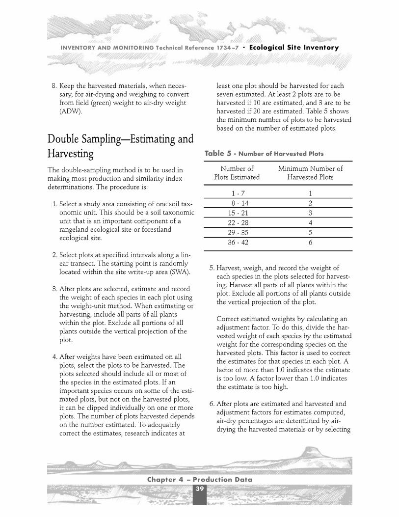
INVENTORY AND MONITORING Technical Reference 1734–7 • Ecological Site Inventory
Chapter 4 – Production Data39
8. Keep the harvested materials, when neces-sary, for air-drying and weighing to convertfrom field (green) weight to air-dry weight(ADW).
Double Sampling—Estimating andHarvestingThe double-sampling method is to be used inmaking most production and similarity indexdeterminations. The procedure is:
1. Select a study area consisting of one soil tax-onomic unit. This should be a soil taxonomicunit that is an important component of arangeland ecological site or forestlandecological site.
2. Select plots at specified intervals along a lin-ear transect. The starting point is randomlylocated within the site write-up area (SWA).
3. After plots are selected, estimate and recordthe weight of each species in each plot usingthe weight-unit method. When estimating orharvesting, include all parts of all plantswithin the plot. Exclude all portions of allplants outside the vertical projection of theplot.
4. After weights have been estimated on allplots, select the plots to be harvested. Theplots selected should include all or most ofthe species in the estimated plots. If animportant species occurs on some of the esti-mated plots, but not on the harvested plots,it can be clipped individually on one or moreplots. The number of plots harvested dependson the number estimated. To adequatelycorrect the estimates, research indicates at
least one plot should be harvested for eachseven estimated. At least 2 plots are to beharvested if 10 are estimated, and 3 are to beharvested if 20 are estimated. Table 5 showsthe minimum number of plots to be harvestedbased on the number of estimated plots.
Table 5 - Number of Harvested Plots
Number of Minimum Number ofPlots Estimated Harvested Plots
1 - 7 18 - 14 2
15 - 21 322 - 28 429 - 35 536 - 42 6
5. Harvest, weigh, and record the weight ofeach species in the plots selected for harvest-ing. Harvest all parts of all plants within theplot. Exclude all portions of all plants outsidethe vertical projection of the plot.
Correct estimated weights by calculating anadjustment factor. To do this, divide the har-vested weight of each species by the estimatedweight for the corresponding species on theharvested plots. This factor is used to correctthe estimates for that species in each plot. Afactor of more than 1.0 indicates the estimateis too low. A factor lower than 1.0 indicatesthe estimate is too high.
6. After plots are estimated and harvested andadjustment factors for estimates computed,air-dry percentages are determined by air-drying the harvested materials or by selecting

INVENTORY AND MONITORING Technical Reference 1734–7 • Ecological Site Inventory
Chapter 4 – Production Data40
the appropriate factor from an air-dry per-centage table (Appendix 7). Values for eachspecies are then corrected to air-dry poundsper acre or kilograms per hectare for all plots.Average weight and percentage compositioncan then be computed for the sample area.
Plot SizeAdapt the size and shape of plots to the kind ofplants to be sampled. The area of a plot can beexpressed in square feet, inches and meters, or inacres.
If vegetation is relatively short, the followingplot sizes work best in determining production:
0.96 ft2 or 41.7 inch circumference1.92 ft2 or 59 inch circumference2.40 ft2 or 66 inch circumference4.80 ft2 or 93.2 inch circumference9.60 ft2 or 131.8 inch circumference
The listed plots are the most useful when con-verting grams to pounds per acre. The 9.6 ft2 plotis generally used in areas where vegetationdensity and production are relatively light. Thesmaller plots, especially the 0.96 ft2 and 1.92 ft2
plots, are satisfactory in areas of homogeneous,relatively dense vegetation like that occurring inmeadows. Plots larger than 9.6 ft2 should be usedwhere vegetation is very sparse and heterogeneous.
If the vegetation consists of trees or large shrubs,larger plots must be used. If the tree or shrubpopulation is uniform, a 0.01 acre plot is moresuitable. If vegetation is unevenly spaced, a moreaccurate sample can be obtained by using a 0.1acre plot, 4.356 feet wide and 1,000 feet long.For statistical analyses, 10 plots of 0.01 acre aresuperior to a single 0.1 acre plot. Plots of 0.1 and
0.01 acre are most useful when productiondata is collected in pounds because it is a directconversion.
If vegetation is mixed, two sizes of plots generallyare needed. A series of 10 square or rectangularplots of 0.01 acre and a smaller plot, such as the9.6-square-foot plot nested in a designated cor-ner of each larger plot, is suitable. The 0.01-acreplot is used for trees or large shrubs, and thesmaller plot for lower-growing plants. Weights ofthe vegetation from both plots are then convertedto pounds per acre. Plots with area expressed insquare meters are used if production is to bedetermined in kilograms per hectare.
If the plots are nested, production from bothplots must be recorded in the same units ofmeasure. For example, a plot 20 meters by 20meters (or other dimensions that equal 400meters) can be used for measuring the tree andshrub vegetation and a 1-meter plot nested in adesignated corner can be used for measuring thelow-growing plants. Determine the productionfrom both in grams and convert the grams tokilograms per hectare. Plots of 0.25, 1, 10, 100,and 400 square meters are commonly used.
Plot ShapePlots can be circular, square, or rectangular.However, long-narrow plots are likely to be moreaccurate than circular, square, or rectangularplots (Krebs 1989). Edge effect can result insignificant measurement bias if the plots are toosmall (Wiegert 1962). Since aboveground vegeta-tion must be clipped in some plots, circular plotsshould be avoided because of the difficulty incutting around the perimeter of the circle withhand shears and the likely measurement biasthat would result.
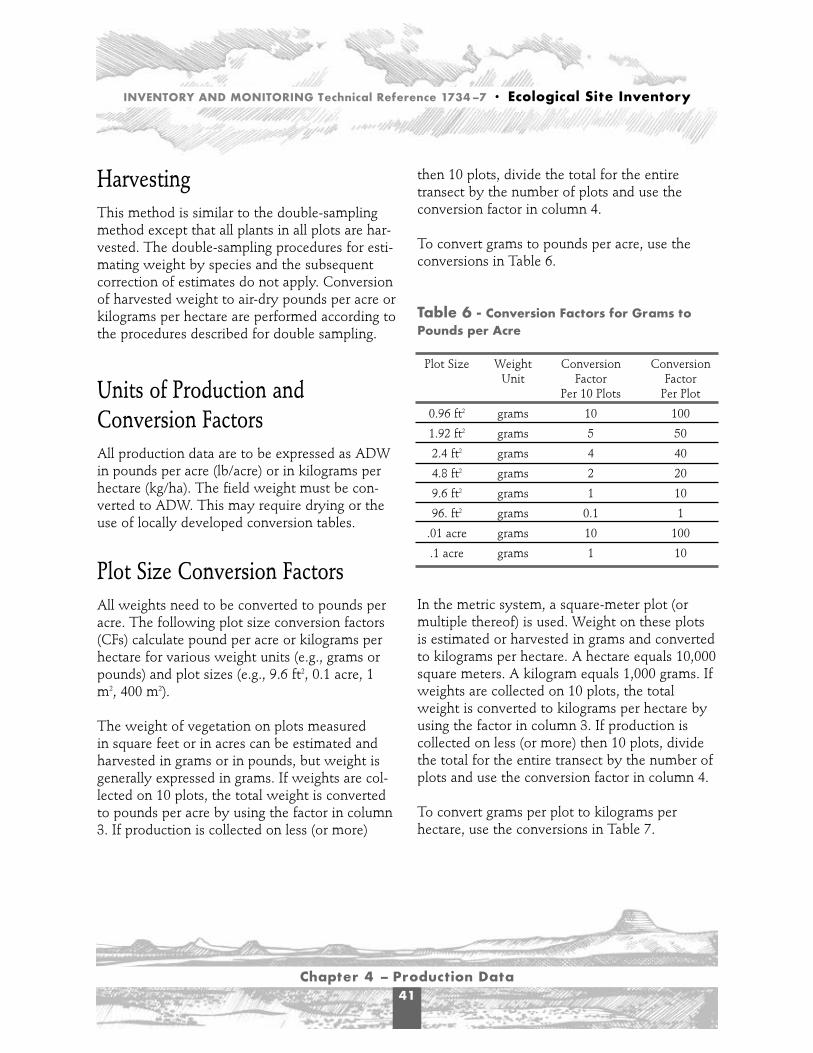
INVENTORY AND MONITORING Technical Reference 1734–7 • Ecological Site Inventory
Chapter 4 – Production Data41
HarvestingThis method is similar to the double-samplingmethod except that all plants in all plots are har-vested. The double-sampling procedures for esti-mating weight by species and the subsequentcorrection of estimates do not apply. Conversionof harvested weight to air-dry pounds per acre orkilograms per hectare are performed according tothe procedures described for double sampling.
Units of Production andConversion FactorsAll production data are to be expressed as ADWin pounds per acre (lb/acre) or in kilograms perhectare (kg/ha). The field weight must be con-verted to ADW. This may require drying or theuse of locally developed conversion tables.
Plot Size Conversion FactorsAll weights need to be converted to pounds peracre. The following plot size conversion factors(CFs) calculate pound per acre or kilograms perhectare for various weight units (e.g., grams orpounds) and plot sizes (e.g., 9.6 ft2, 0.1 acre, 1m2, 400 m2).
The weight of vegetation on plots measuredin square feet or in acres can be estimated andharvested in grams or in pounds, but weight isgenerally expressed in grams. If weights are col-lected on 10 plots, the total weight is convertedto pounds per acre by using the factor in column3. If production is collected on less (or more)
then 10 plots, divide the total for the entiretransect by the number of plots and use theconversion factor in column 4.
To convert grams to pounds per acre, use theconversions in Table 6.
Table 6 - Conversion Factors for Grams toPounds per Acre
Plot Size Weight Conversion ConversionUnit Factor Factor
Per 10 Plots Per Plot
0.96 ft2 grams 10 100
1.92 ft2 grams 5 50
2.4 ft2 grams 4 40
4.8 ft2 grams 2 20
9.6 ft2 grams 1 10
96. ft2 grams 0.1 1
.01 acre grams 10 100
.1 acre grams 1 10
In the metric system, a square-meter plot (ormultiple thereof) is used. Weight on these plotsis estimated or harvested in grams and convertedto kilograms per hectare. A hectare equals 10,000square meters. A kilogram equals 1,000 grams. Ifweights are collected on 10 plots, the totalweight is converted to kilograms per hectare byusing the factor in column 3. If production is collected on less (or more) then 10 plots, dividethe total for the entire transect by the number ofplots and use the conversion factor in column 4.
To convert grams per plot to kilograms perhectare, use the conversions in Table 7.

INVENTORY AND MONITORING Technical Reference 1734–7 • Ecological Site Inventory
Chapter 4 – Production Data42
Table 7 - Conversion Factors for Grams toKilograms per Hectare
Plot Size Weight Conversion ConversionUnit Factor Factor
Per 10 Plots Per Plot
0.25 m2 grams 10 100
1 m2 grams 10 100
10 m2 grams 10 100
100 m2 grams 10 100
400 m2 grams 10 100
Mixed Measuring UnitsWith large volumes of vegetative material associ-ated with trees and large shrubs, it is more prac-tical to estimate weights in pounds rather thangrams. The conversion factor on a per plot basis,when weights are collected in pounds for a 96 ft2
plot, is 454. Likewise, vegetative material associ-ated with grasses, forbs, and small shrubs ismore easily estimated in grams. Therefore, on aper plot basis, weights collected in grams for a .1acre plot would convert to 2.2 pounds per acre(conversion for a 0.01 acre plot is 0.22).
Adjustment FactorsThe ideal situation for determining productiondata for each individual species is to samplethem when they are at their maximum produc-tion. With a diversity of species, it is impossibleto make these determinations at one point intime during the growing season. Therefore, theproduction of each species must be reconstructedto reflect total annual production. This is accom-plished using the conversion factors describedpreviously.
Green Weight Adjustment FactorThis is the procedure for converting green weight,which is the weight of vegetation estimated orcollected in the field, to air-dry weight.
ADW percentages for various types of plantsat different stages of growth are provided inAppendix 7. These percentages are based on cur-rently available data and are intended for interimuse. As additional data from field evaluationsbecome available, these figures will be revised.ADW percentages listed in Appendix 7 can beused for other species having growth characteristicssimilar to those of the species listed.
States that have prepared their own tables ofair-dry percentages on the basis of actual fieldexperience can substitute them for the tables inAppendix 7. Be sure to check with the localoffice of the NRCS for their latest ADW percent-age tables. It is recommended that local fieldoffices develop these tables for local conditionsand species. Some interpolation must be done inthe field to determine air-dry percentages forgrowth stages other than those listed. If ADWpercentage figures have not been previouslydetermined and included in ADW percentagetables, or if ADW conversion factors need to bechecked, retain and dry enough harvested materialsamples to determine ADW percentages.
The relationship of green weight to ADW variesaccording to such factors as exposure, amount ofshading, time since last rain, and unseasonabledry periods. Several samples of plant materialshould be harvested and air-dried each season toverify the factors shown in Appendix 7 or toestablish factors for local use.
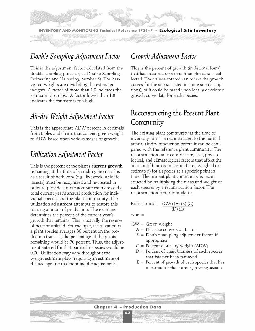
INVENTORY AND MONITORING Technical Reference 1734–7 • Ecological Site Inventory
Chapter 4 – Production Data43
Double Sampling Adjustment Factor This is the adjustment factor calculated from thedouble sampling process (see Double Sampling—Estimating and Havesting, number 6). The har-vested weights are divided by the estimatedweights. A factor of more than 1.0 indicates theestimate is too low. A factor lower than 1.0indicates the estimate is too high.
Air-dry Weight Adjustment FactorThis is the appropriate ADW percent in decimalsfrom tables and charts that convert green weightto ADW based upon various stages of growth.
Utilization Adjustment FactorThis is the percent of the plant’s current growthremaining at the time of sampling. Biomass lostas a result of herbivory (e.g., livestock, wildlife,insects) must be recognized and re-created inorder to provide a more accurate estimate of thetotal current year’s annual production for indi-vidual species and the plant community. Theutilization adjustment attempts to restore thismissing amount of production. The examinerdetermines the percent of the current year’sgrowth that remains. This is actually the reverseof percent utilized. For example, if utilization ona plant species averages 30 percent on the pro-duction transect, the percentage of the plantsremaining would be 70 percent. Thus, the adjust-ment entered for that particular species would be0.70. Utilization may vary throughout theweight estimate plots, requiring an estimate ofthe average use to determine the adjustment.
Growth Adjustment FactorThis is the percent of growth (in decimal form)that has occurred up to the time plot data is col-lected. The values entered can reflect the growthcurves for the site (as listed in some site descrip-tions), or it could be based upon locally developedgrowth curve data for each species.
Reconstructing the Present PlantCommunityThe existing plant community at the time ofinventory must be reconstructed to the normalannual air-dry production before it can be com-pared with the reference plant community. Thereconstruction must consider physical, physio-logical, and climatological factors that affect theamount of biomass measured (i.e., weighed orestimated) for a species at a specific point intime. The present plant community is recon-structed by multiplying the measured weight ofeach species by a reconstruction factor. Thereconstruction factor formula is:
Reconstructed (GW) (A) (B) (C) (D) (E)
where:
GW = Green weightA = Plot size conversion factorB = Double sampling adjustment factor, if
appropriate C = Percent of air-dry weight (ADW)D = Percent of plant biomass of each species
that has not been removedE = Percent of growth of each species that has
occurred for the current growing season

INVENTORY AND MONITORING Technical Reference 1734–7 • Ecological Site Inventory
Chapter 4 – Production Data44
Ocular Estimation of ProductionData Ocular estimates of production for an entire site,as opposed to estimating production on individualplots, is the quickest and easiest technique.However, with inexperienced people, thereduced accuracy resulting from this techniquelimits the use of the data. Ocular estimates areuseful in quickly determining the similarityindex of a site (see Chapter 5) for use in mappingplant communities and in stratifying SWAs forsampling purposes.
The following procedure is used in to becomeproficient at estimating production for an SWA.
1. Estimate production, in pounds per acre orkilograms per hectare, of individual specieson the site.
2. Estimate production of individual species ona series of random plots.
3. Compute production in pounds per acre orkilograms per hectare from the random plots.To further check these estimates, harvest ordouble sample according to proceduresaddressed in the double sampling section ofthis document.
4. Repeat procedure until proficiency isattained.
Although this procedure misses some species ofminor importance, it provides a useful check onestimates.
Inventory Level of IntensityThe minimum standard for an ecological siteinventory is production by species. The level orintensity at which the production of a plantcommunity is determined depends on theintended use of the data. Ocular estimates arethe quickest and easiest technique for determiningproduction, but may result in reduced accuracy,limiting use of the data. Estimating production ofindividual species on production plots is moretime consuming, but the accuracy of the data issignificantly increased, especially if plots areperiodically harvested and weight-unit weightsare adjusted accordingly. Harvesting is the mostaccurate technique, but because of the additionaltime required for collection is seldom usedexcept in research-type efforts. A combination ofharvesting and estimating or double sampling isprobably the best technique for documenting theproduction on the site. Double sampling is thetechnique NRCS uses for documenting newecological site descriptions and revising existingdescriptions. Even with the estimating technique,frequent clipping studies (harvesting) should beconducted to calibrate the observer’s eye.
Production Data for DocumentingRangeland Ecological SitesData to be used for preparing rangeland ecologi-cal site descriptions and grouping soils intorangeland ecological sites are to be obtained bythe double-sampling procedure. All documentedproduction and composition data are to berecorded on the Vegetation ProductionWorksheet in Appendix 4. Specific proceduresfor documenting an ecological site descriptioncan be found in the NRSC National Range andPasture Handbook, Chapter 4.

T
INVENTORY AND MONITORING Technical Reference 1734–7 • Ecological Site Inventory
Chapter 5 – Similarity Index45
Definition and Purpose of aSimilarity IndexTHE PRESENT PLANT COMMUNITY on anecological site can be compared to a referencecommunity by the calculation of a similarityindex. In most cases, the reference community isthe historic climax plant community or potentialnatural community.
A similarity index is a comparison of the presentstate of vegetation on an ecological site in rela-tion to the kinds, proportions, and amounts ofvegetation with other vegetation communitiesthe site is capable of producing. It is expressed asthe percentage of a plant community that ispresently on the site. To make the comparison,the reference vegetation communities must bedescribed in sufficient detail in the ecological sitedescription. As ecological site descriptions arerevised and further developed, they should alsoinclude descriptions of other common vegetationcommunities that can exist on the site.
The similarity index can provide managers witha starting point for establishing specific manage-ment objectives. It also provides a means ofdetermining the successional status (Table 8).
Table 8 - Successional Status
Similarity SuccessionalIndex Status
0-25% early26-50% mid51-76% late77-100% (potential natural community)
Determining Similarity Index A similarity index determines how closely thecurrent plant community resembles either thepotential natural community or some other refer-ence community. In order to make this determi-nation, the existing plant community must beinventoried by recording weight, in pounds peracre, for each species present. In determining thesimilarity index, the allowable production of aspecies in the existing plant community cannotexceed the production of the species in the refer-ence plant community. If plant groups are used,the present reconstructed production of a groupcannot exceed the production of the group in thereference plant community.
Table 9 demonstrates how the similarity index isdetermined on four different reference communi-ties for a loamy upland 12-16 PZ ecological site.(Refer to Chapter 3 for information on EcologicalSites and Appendix 3 for the ecological sitedescription.) Table 9 shows only one plant fromeach plant group described in the ecological sitedescription. This is for illustrative purposes toshow the calculation of the similarity index. Inactual practice, it is desirable to list all speciesfound on the sample transect. This exampleassumes the current plant community has beenreconstructed to actual annual production.
Chapter 5 - Similarity Index

INVENTORY AND MONITORING Technical Reference 1734–7 • Ecological Site Inventory
Chapter 5 – Similarity Index46
On the similarity index form in Table 9, eachspecies is listed in column B, along with theproduction for the reference plant community incolumn C (pounds per acre). Current annual pro-duction for each species is shown in column D.The allowable production in column E is deter-mined by using the smaller of the two production
amounts (columns B or C). The total allowableproduction represents the amount of the refer-ence plant community that is currently presenton the site. The similarity index is determinedby dividing the total allowable production (totalof column E) by the total production for thereference community (total of column C).
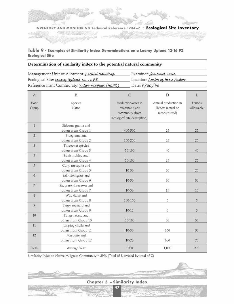
INVENTORY AND MONITORING Technical Reference 1734–7 • Ecological Site Inventory
Chapter 5 – Similarity Index47
Table 9 - Examples of Similarity Index Determinations on a Loamy Upland 12-16 PZEcological Site
Determination of similarity index to the potential natural community
Management Unit or Allotment: Rockin’ Raindrop Examiner: Someone’s name
Ecological Site: Loamy Upland 12-16 PZ Location: Center of Horse Pasture
Reference Plant Community: Native midgrass (HCPC) Date: 8/30/96
A B C D E
Plant Species Production/acres in Annual production in Pounds
Group Name reference plant lb/acre (actual or Allowable
community (from reconstructed)
ecological site description)
1 Sideouts grama and
others from Group 1 400-500 25 25
2 Bluegrama and
others from Group 2 150-250 25 25
3 Threeawn species
others from Group 3 50-100 40 40
4 Bush muhley and
others from Group 4 50-100 25 25
5 Curly mesquite and
others from Group 5 10-50 20 20
6 Fall witchgrass and
others from Group 6 10-50 30 30
7 Six week threeawn and
others from Group 7 10-50 15 15
8 Wild daisy and
others from Group 8 100-150 5 5
9 Tansy mustard and
others from Group 9 10-15 5 5
10 Range ratany and
others from Group 10 50-100 50 50
11 Jumping cholla and
others from Group 11 10-50 160 30
12 Mesquite and
others from Group 12 10-20 600 20
Totals Average Year 1000 1,000 290
Similarity Index to Native Midgrass Community = 29% (Total of E divided by total of C)

INVENTORY AND MONITORING Technical Reference 1734–7 • Ecological Site Inventory
Chapter 5 – Similarity Index48
Table 9 - (continued)
Determination of similarity index to the mesquite-short grass vegetation stateon loamy upland 12-16 PZ site
Management Unit or Allotment: Rockin’ Raindrop Examiner: Someone’s nameEcological Site: Loamy Upland 12-16 PZ Location: Center of Horse Pasture
Reference Plant Community: Mesquite-Short Grass Date: 8/30/96
A B C D E
Plant Species Production/acres in Annual production in Pounds
Group Name reference plant lb/acre (actual or Allowable
community (from reconstructed)
ecological site description)
1 Sideouts grama and
others from Group 1 15-50 25 25
2 Bluegrama and
others from Group 2 300-400 25 25
3 Threeawn species and
others from Group 3 10-50 40 40
4 Bush muhley and
others from Group 4 0 25 0
5 Curly mesquite and
others from Group 5 15-100 20 20
6 Fall witchgrass and
others from Group 6 0 30 0
7 Six week threeawn and
others from Group 7 0 15 0
8 Wild daisy and
others from Group 8 10-50 5 5
9 Tansy mustard and
others from Group 9 0 5 0
10 Range ratany and
others from Group 10 10-50 50 50
11 Jumping cholla and
others from Group 11 0 160 0
12 Mesquite and
others from Group 12 15-100 600 100
TOTALS 665 1,000 265
Similarity Index to Mesquite-Short Grass Community = 40% (Total of E divided by total of C)

INVENTORY AND MONITORING Technical Reference 1734–7 • Ecological Site Inventory
Chapter 5 – Similarity Index49
Table 9 - (continued)
Determination of similarity index to the native-short grass vegetation stateon loamy upland 12-16 PZ site
Management Unit or Allotment: Rockin’ Raindrop Examiner: Someone’s name
Ecological Site: Loamy Upland 12-16 PZ Location: Center of Horse Pasture
Reference Plant Community: Native-Short Grass Date: 8/30/96
A B C D E
Plant Species Production/acres in Annual production in Pounds
Group Name reference plant lb/acre (actual or Allowable
community (from reconstructed)
ecological site description)
1 Sideouts grama and
others from Group 1 15-50 25 25
2 Bluegrama and
others from Group 2 300-400 25 25
3 Threeawn species and
others from Group 3 15-50 40 40
4 Bush muhley and
others from Group 4 0 25 0
5 Curly mesquite and
others from Group 5 15-150 20 20
6 Fall witchgrass and
others from Group 6 0 30 0
7 Six week threeawn and
others from Group 7 0 15 0
8 Wild daisy and
others from Group 8 15-50 5 5
9 Tansy mustard and
others from Group 9 0 5 0
10 Range ratany and
others from Group 10 15-50 50 50
11 Jumping cholla and
others from Group 11 trace 160 0
12 Mesquite and
others from Group 12 trace 600 0
TOTALS 630 1,000 165
Similarity Index to Native-Short Grass Community = 26% (Total of E divided by total of C)

INVENTORY AND MONITORING Technical Reference 1734–7 • Ecological Site Inventory
Chapter 5 – Similarity Index50
Table 9 - (continued)
Determination of similarity index to dense mesquite vegetation stateon loamy upland 12-16 PZ site
Management Unit or Allotment: Rockin’ Raindrop Examiner: Someone’s name
Ecological Site: Loamy Upland 12-16 PZ Location: Center of Horse Pasture
Reference Plant Community: Dense Mesquite Date: 8/30/96
A B C D E
Plant Species Production/acres in Annual production in Pounds
Group Name reference plant lb/acre (actual or Allowable
community (from reconstructed)
ecological site description)
1 Sideouts grama and
others from Group 1 0 25 0
2 Bluegrama and
others from Group 2 0 25 0
3 Threeawn species and
others from Group 3 15-50 40 40
4 Bush muhley and
others from Group 4 15-50 25 25
5 Curly mesquite and
others from Group 5 0 20 0
6 Fall witchgrass and
others from Group 6 0 30 0
7 Six week threeawn and
others from Group 7 0 15 0
8 Wild daisy and
others from Group 8 0 5 0
9 Tansy mustard and
others from Group 9 0 5 0
10 Range ratany and
others from Group 10 0 50 0
11 Jumping cholla and
others from Group 11 0 160 0
12 Mesquite and
others from Group 12 500-600 600 555
TOTALS 620 1,000 620
Similarity Index to Native-Short Grass Community = 100% (Total of E divided by total of C)
(Table adapted from the NRCS National Range and Pasture Handbook, 1997)

INVENTORY AND MONITORING Technical Reference 1734–7 • Ecological Site Inventory
Chapter 5 – Similarity Index51
Many older ecological site descriptions docu-ment the extent of individual species within thehistoric climax plant community by percent ofcomposition rather than pounds per acre.Production figures are presented as total weights(pounds per acre) for normal years, favorableyears, and unfavorable years.
To calculate a similarity index, species composi-tion must be converted to pounds per acre.Because the percent of composition for eachspecies is based on total air-dry weight (ADW),
conversion of the percentages to pounds per acreis easy. Simply multiply the percentage for eachspecies by the total pounds per acre for an aver-age year to arrive at the number of pounds peracre for each species. Table 10 converts the per-cent composition (column 2) from the referencecommunity (found in an ecological site descrip-tion) to pounds per acre (column 3). Also shownis the annual production (column 4) and theallowable production (column 5). Column 5 isdetermined by the smaller of the two amounts(column 3 or 4).
Table 10 - Reference Community
Reference Community
Symbol % of PNC (Reference Average Year Annual AllowableCommunity) 1000 lbs/acre Production Production
Grasses 75-85 750/850 180 180Group 1 40/50 400-500 25 25Group 2 15-25 150-250 25 25Group 3 5-10 50-100 40 40Group 4 1-5 10-50 25 25Group 5 1-5 10-50 20 20Group 6 1-5 10-50 30 30Group 7 1-5 10-50 15 15Forbs 5-10 50-100 10 10Group 8 10-15 100-150 5 5Group 9 1-5 10-50 5 5Shrubs/Trees 5-10 50-100 810 100Group 10 5-10 50-100 50 50Group 11 1-5 10-50 160 30Group 12 1-2 10-20 600 20
INVENTORY AND MONITORING Technical Reference 1734–7 • Ecological Site Inventory
Chapter 5 – Similarity Index52
In determining allowable production, it is impor-tant not to exceed the production of the refer-ence community relative to each species, plantgroup, or life form. In Table 10, the annual pro-duction of plant groups 1 through 10 does notexceed production in the reference community.In addition, the total annual production of grass-es and forbs does not exceed production in thereference community.
In plant groups 11 and 12, annual production ismuch higher than allowed in the reference com-munity. Therefore, the most production that canbe credited is 50 and 20 pounds per acre respec-tively (high end of column 3). It is also importantnot to exceed the allowable production for allshrubs and trees (groups 10, 11, and 12).However, the total annual production for allshrubs and trees is 810 pounds and the allowableproduction is 100 pounds. Since plant group 10has already been credited with the 50 poundsallowable, the remaining plant groups (11 and12) can total no more than 50 pounds. Group 12is given credit for 20 pounds, leaving 30 poundsfor group 11.
Determining Similarity Index tothe Potential Natural CommunityWhen compared to the potential natural commu-nity, the similarity index represents the percentof the potential natural community present onthe site. This provides a basis for describing theextent and direction of change that has occurred.The similarity index, coupled with the state andtransition model, can help predict changes thatcould occur.
Determining Similarity Index toOther Vegetation States orDesired Plant CommunityDetermining the similarity index of the existingplant community to one or more of the possiblevegetation states in the site description may bedesirable. After management objectives havebeen developed, one specific plant communitymay be identified as the desired plant communi-ty. Once the desired plant community has beenidentified, it is appropriate to determine the sim-ilarity index of the existing community to thedesired plant community.
Procedures for determining a similarity index forother vegetation communities are the same asdescribed for the historic climax plant communi-ty. Table 9 shows similarity index determinationsfor some of the other vegetation states describedin the loamy upland 12-16 PZ. These determina-tions use the same transect data used in Table 9.Refer to Chapter 3 for information on ecologicalsites and Appendix 3 for the ecological sitedescription. These examples show only onespecies from each plant group.

T
INVENTORY AND MONITORING Technical Reference 1734–7 • Ecological Site Inventory
Chapter 6 – Field Procedures53
Minimum StandardsTHE MINIMUM STANDARDS REQUIRED foran ecological site inventory are production andcomposition by air-dry weight (ADW) byspecies. The number of plots selected dependson the purpose for which the estimates are to beused, uniformity of the vegetation, and otherfactors. A minimum of 10 plots should be select-ed for collecting production data used in docu-menting rangeland ecological sites or for otherinterpretive purposes. If vegetation distribution isvery irregular and 10 plots will not give an ade-quate sampling, additional plots can be selected.If the inventory design dictates it, fewer than 10plots can be used.
Sampling PrecisionMost uses of ecological site inventory datawould not require the calculation of a samplesize necessary to achieve a given level of preci-sion at a given confidence level. Quantitativemonitoring studies would be one situationrequiring this calculation. However, if an inven-tory plan calls for a specified level of precision,refer to Sample Size Equation number 1, pages346–350 of Measuring and Monitoring PlantPopulations, BLM Technical Reference 1730-1.To use this equation (or the software programdiscussed in the next paragraph), an estimate ofthe standard deviation is needed. This can beobtained by taking an initial sample of quadratsand calculating the standard deviation of the setof total production values obtained from this
sample. The standard deviation of a set of valuesis easily calculated using the statistics mode orfunction on a hand calculator configured withthat option or by using the standard deviationformula (also called “worksheet function”) on acomputer spreadsheet (e.g., the appropriateformula in Microsoft Excel is STDEV).
The easiest way to calculate the sample size foran ecological site inventory is to use the free-ware program, PC SIZE: Consultant, which runson any DOS or Windows machine. Instructionson obtaining and using it are given at the Website associated with the book, Monitoring Plantand Animal Populations: A Handbook for FieldBiologists by C. L. Elzinga, D. W. Salzer, J. W.Willoughby, and J. P. Gibbs, Blackwell ScienceInc., 2001, at
http://www.esf.edu/course/jpgibbs/monitor/popmonroot.html
Once there, click on “Chapter 9, Statistics,” thenon “Instructions for Using DTSTPLAN and PC-SIZE: Consultant to Estimate Sample Size andConduct Post Hoc Power Analyses.” You'll thenget a PDF file that tells how to download PCSIZE: Consultant and how to use it.
Site Write-up AreaFor sampling and planning purposes, the land-scape is divided into map units called site write-up
Chapter 6 - Field Procedures

INVENTORY AND MONITORING Technical Reference 1734–7 • Ecological Site Inventory
Chapter 6 – Field Procedures54
areas (SWAs). A SWA is defined as the smallestgeographical unit delineation to be used as abase for collecting vegetation data and resourceinformation. It is the smallest mapped soil- vege-tation unit. SWA delineations are the culminationof mapping ecological sites, vegetation commu-nities, and administrative boundaries. Each indi-vidual SWA should consist of only one ecologicalsite and one plant community. The only exceptionwould be if two or more soil- vegetationcomplexes are so intermingled that individualecological sites cannot be delineated. SWAs maybe mapped down to a minimum of 6 acres.Within a single soil-vegetation unit (ecologicalsite and plant community), for managementpurposes, SWA boundaries can be set on admin-istrative boundaries such as allotments, pastures,wildlife habitat areas, or watersheds. The exactcriteria for subdividing on administrative boundarylines must be documented in the inventory plan.
In order to compile data on a management unitor grazing allotment basis, SWAs must not crossaccurately located management unit or allotmentboundaries. SWAs may also be delineated on soilmapping unit or pasture boundaries as specifiedin the inventory plan. The more detailed themapping, the greater the options are for interpre-tation of the data. A unique SWA number isassigned to each SWA delineated. The numberconsists of one alpha character and a consecutive3 digit number (e.g., A001, F139, S091).
Field Inventory MappingMapping must be done by trained vegetationspecialists, wildlife biologists, foresters, soilscientists, and hydrologists (for riparian areas)
working closely together. Field mapping consistsof delineating SWAs based on present plant com-munities (e.g., ecological sites, forestland ecologi-cal sites, or forest types). Field mapping shouldbe completed prior to resource data collection. Ifthe inventory plan identifies the need to stratifySWAs for vegetation data collection, the entireinventory area must be mapped first. It is desirableto complete mapping a year in advance ofcollecting vegetation data.
Mapping Process With aCompleted Soil SurveyIn areas where soil survey and ecological sitedescriptions are complete, an ecological site-soilseries correlation should be available in the finalsoil survey report. The survey report may alsoidentify soil series that support forestland eco-logical sites or forest types (habitat types) wherethe potential plant communities have alreadybeen defined.
Where Order II soil surveys are completed andecological site interpretations have been made,boundaries of ecological sites can generally bedetermined directly from the soil map.
Order III mapping describes individual soil andplant components at association or complexlevels. Mapping unit descriptions have beendeveloped that describe each association compo-nent and include locations on the landscape andpercentages of each soil. Individual ecologicalsites must be delineated if individual soils in theassociation have different potential historic climaxplant communities.

INVENTORY AND MONITORING Technical Reference 1734–7 • Ecological Site Inventory
Chapter 6 – Field Procedures55
Mapping Process Without aCompleted Soil SurveyIn areas where soil surveys are not completed,the NRCS must be contacted to obtain any avail-able soil or ecological site data. The NRCS maybe able to assist in training and in establishingthe mapping legend. The mapping team mustwork together in the field to achieve consistencyin SWA delineation based upon ecological sites,forestland ecological sites, or forest types. Thesoil scientist must ensure that soils are consid-ered in delineations. If at all possible, a soil sur-vey should be completed prior to or concurrentlywith delineation of ecological sites.
Mapping Ecological Sites The first step in mapping SWAs is the mappingof ecological sites. Based on soils informationand field reconnaissance, ecological sites aredelineated on aerial photos.
Present VegetationEcological sites are subdivided based on changesin plant communities. Significant changes in thefollowing factors must be considered in delineatingpresent vegetation communities:
1. Vegetation species composition (kinds, pro-portions, and amounts of present vegetation)
2. Vegetation ground cover3. Vegetation height4. Vegetation age class (especially in forested
areas)5. Topography6. Other factors identified in the inventory plan
To assist in this effort, current vegetation com-munities can be mapped as standard vegetationsubtypes. Vegetation types are designatedaccording to vegetation aspect. A complete list-ing is given in Appendix 8. Table 11 lists some ofthe more common types.
Table 11 - Common Standard VegetationSubtypes
Type Subtype Code
Grass Short Grass 1001
Mid Grass 1002
Tall Grass 1003
Grasslike Sedge 2001
Rush 2002
Perennial Forbs Perennial Forbs 3001
Shrub Black Greasewood 4001
Creosote Bush 4011
Winterfat 4015
Mesquite 4021
Saltbush 4030
Mixed Desert Shrub 4037
Sagebrush 4040
Mtn. Mahogany 4056
Bitterbrush 4057
Mountain Shrub 4060
Snakeweed 4071
Broadleaf Trees 5000
Conifers 6000
Pinyon 6097
Juniper 6098
Broadleaf Trees Willow 5074
Conifer Douglas Fir 6001
Cryptogams 7000
Barren 8000
Annual Grass 9000
Other 9999

INVENTORY AND MONITORING Technical Reference 1734–7 • Ecological Site Inventory
Chapter 6 – Field Procedures56
Successional Status ClassificationIf appropriate, ecological sites should be furthersubdivided based on the successional status ofthe existing plant community. This is usuallyapparent on the ground as a change in the plantcommunity. Each distinct soil-vegetation unitshould be placed in a successional status class bymaking visual estimates of species production(see ocular estimation of production data inChapter 4). The mapping team should completethe Similarity Index Form (Appendix 9) to recordthese initial successional status determinations.To make this initial determination of successionstatus, compare the present plant communitywith that of the potential natural community.For the existing plant community, count asallowable production no more than the maxi-mum weight shown on the ecological sitedescription for any species in the climax commu-nity. Total the allowable production of all poten-tial natural community species to indicate therelative similarity index. The rating must bebetween 0 and 100, depending on how closelythe existing plant community resembles thepotential natural community for the ecologicalsite. These estimated similarity indices can beuseful in a stratification effort.
Forest Types Forest types are divided into stands—uniformplant communities of trees as to timber type, ageclass, vigor, height, ground cover, and stocking.The smallest delineated unit within a forest typeis the SWA or stand. The mapping team mustassign a SWA number to each delineated SWA.
Feature Mapping Any permanent cultural, topographic, and bio-logical features, as well as existing improvements,such as fences, roads, or water developments notshown on existing maps should be indicated onaerial photographs. Barriers to livestock, wildlife,or wild horse and burros should be noted.
Water ResourcesShow all water resources, such as marshes,reservoirs, springs, seeps, or streams.
Photo ScaleThe recommended standard photo scale for anecological site inventory is 1:24,000. The mini-mum size delineation for SWAs is about 6 acresfor distinct wildlife habitat areas, such as riparianareas for food and cover and cliffs or promontoriesfor raptors. Table 12 shows minimum sizedelineations.
Table 12 - Photo Scale Minimum SizeDelineations
Scale Acres Inches/Miles
1:20,000 4.0 3.161:24,000 6.0 2.641:31,680 10.0 2.0
StratificationStratification is grouping together similar SWAsfor sampling purposes. To be stratified, a SWAmust be composed of similar soil-vegetation
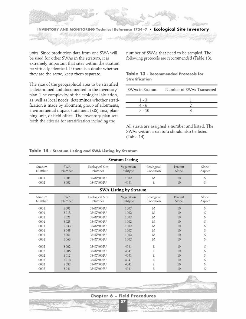
INVENTORY AND MONITORING Technical Reference 1734–7 • Ecological Site Inventory
Chapter 6 – Field Procedures57
units. Since production data from one SWA willbe used for other SWAs in the stratum, it isextremely important that sites within the stratumbe virtually identical. If there is a doubt whetherthey are the same, keep them separate.
The size of the geographical area to be stratifiedis determined and documented in the inventoryplan. The complexity of the ecological situation,as well as local needs, determines whether strati-fication is made by allotment, group of allotments,environmental impact statement (EIS) area, plan-ning unit, or field office. The inventory plan setsforth the criteria for stratification including the
number of SWAs that need to be sampled. Thefollowing protocols are recommended (Table 13).
Table 13 - Recommended Protocols forStratification
SWAs in Stratum Number of SWAs Transected
1 - 3 14 - 6 27 - 10 3
All strata are assigned a number and listed. TheSWAs within a stratum should also be listed(Table 14).
Table 14 - Stratum Listing and SWA Listing by Stratum
Stratum Listing
Stratum SWA Ecological Site Vegetation Ecological Percent Slope Number Number Number Subtype Condition Slope Aspect
0001 B001 034XY001U 1002 M 10 N0002 B002 034XY002U 4041 E 10 N
SWA Listing by Stratum
Stratum SWA Ecological Site Vegetation Ecological Percent Slope Number Number Number Subtype Condition Slope Aspect
0001 B001 034XY001U 1002 M 10 N0001 B013 034XY001U 1002 M 10 N0001 B021 034XY001U 1002 M 10 N0001 B023 034XY001U 1002 M 10 N0001 B033 034XY001U 1002 M 10 N0001 B043 034XY001U 1002 M 10 N0001 B051 034XY001U 1002 M 10 N0001 B063 034XY001U 1002 M 10 N
0002 B002 034XY002U 4041 E 10 N0002 B006 034XY002U 4041 E 10 N0002 B012 034XY002U 4041 E 10 N0002 B018 034XY002U 4041 E 10 N0002 B032 034XY002U 4041 E 10 N0002 B041 034XY002U 4041 E 10 N
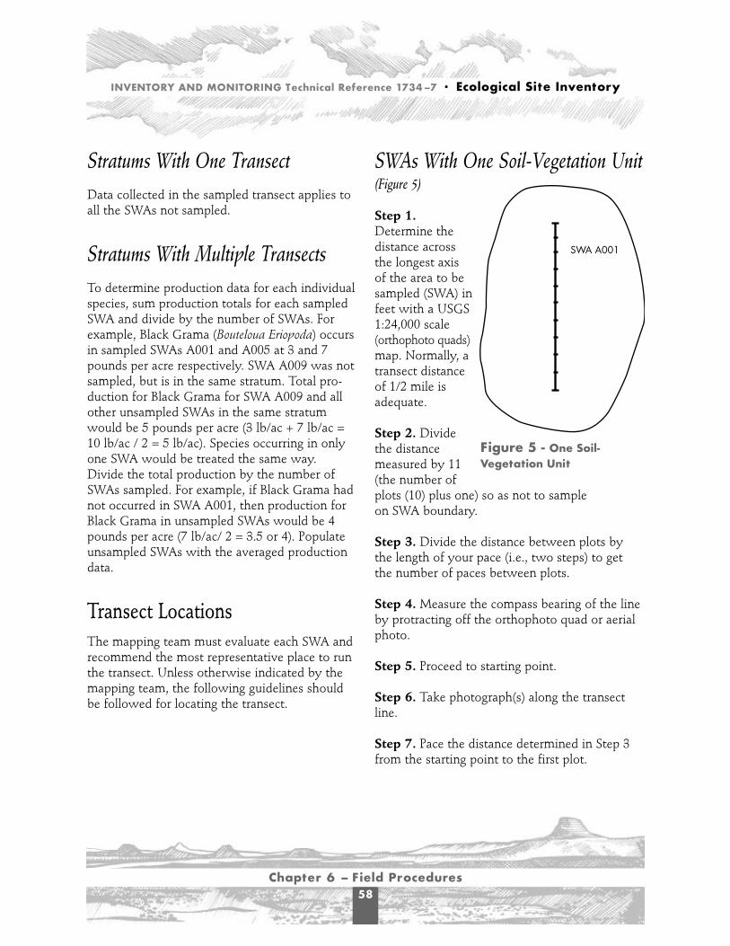
INVENTORY AND MONITORING Technical Reference 1734–7 • Ecological Site Inventory
Chapter 6 – Field Procedures58
Stratums With One TransectData collected in the sampled transect applies toall the SWAs not sampled.
Stratums With Multiple TransectsTo determine production data for each individualspecies, sum production totals for each sampledSWA and divide by the number of SWAs. Forexample, Black Grama (Bouteloua Eriopoda) occursin sampled SWAs A001 and A005 at 3 and 7pounds per acre respectively. SWA A009 was notsampled, but is in the same stratum. Total pro-duction for Black Grama for SWA A009 and allother unsampled SWAs in the same stratumwould be 5 pounds per acre (3 lb/ac + 7 lb/ac =10 lb/ac / 2 = 5 lb/ac). Species occurring in onlyone SWA would be treated the same way.Divide the total production by the number ofSWAs sampled. For example, if Black Grama hadnot occurred in SWA A001, then production forBlack Grama in unsampled SWAs would be 4pounds per acre (7 lb/ac/ 2 = 3.5 or 4). Populateunsampled SWAs with the averaged productiondata.
Transect Locations The mapping team must evaluate each SWA andrecommend the most representative place to runthe transect. Unless otherwise indicated by themapping team, the following guidelines shouldbe followed for locating the transect.
SWAs With One Soil-Vegetation Unit(Figure 5)
Step 1.Determine thedistance acrossthe longest axisof the area to besampled (SWA) infeet with a USGS1:24,000 scale(orthophoto quads)map. Normally, atransect distanceof 1/2 mile isadequate.
Step 2. Dividethe distancemeasured by 11(the number ofplots (10) plus one) so as not to sampleon SWA boundary.
Step 3. Divide the distance between plots bythe length of your pace (i.e., two steps) to getthe number of paces between plots.
Step 4. Measure the compass bearing of the lineby protracting off the orthophoto quad or aerialphoto.
Step 5. Proceed to starting point.
Step 6. Take photograph(s) along the transectline.
Step 7. Pace the distance determined in Step 3from the starting point to the first plot.
SWA A001
Figure 5 - One Soil-Vegetation Unit

INVENTORY AND MONITORING Technical Reference 1734–7 • Ecological Site Inventory
Chapter 6 – Field Procedures59
SWAs With Mixed or MottledPatterns (Figure 6)
Where vegetation units are mixed or mottled, itwill be necessary to randomly select plots in eachsoil-vegetation unit in order to collect a reliablesample. Soil-vegetation Unit A is one soil-vegetation unit that will be sampled by Transect 1.Soil- vegetation Unit B occurs as islands sur-rounded by Unit A. When collecting data forTransect 2, it will be necessary to divide Transect2 into segments and locate some of the 10 plotson each island of Unit B. Both transects arewithin SWA F139.
The percentage of each soil-vegetation unitwithin the SWA is recorded on the VegetationProduction Worksheet in Appendix 4.
Other Options for Transect Layout (Figures 7a and 7b)
This option uses the same procedures used inthe “SWAs With One Soil-Vegetation Unit” sec-tion, except the distance and compass bearing ofeach transect leg will have to be calculated.
1
AB
B
B
SWA F139
2
2
2
Figure 6 - Mixed orMottled Soil-Vegetation Units
SWA S009
Figure 7a - A Two-Legged Transect
SWA D201
Figure 7b - A Multi-Legged Transect

INVENTORY AND MONITORING Technical Reference 1734–7 • Ecological Site Inventory
Chapter 6 – Field Procedures60
Plot Sampling Randomly select the beginning point of the tran-sect. Determine the transect bearing and select aprominent distant landmark such as a peak orrocky point that can be used as the transectbearing point. Production plots are placed at thespecified interval (i.e., paced or measured) alongthe transect bearing.
Vegetation Production WorksheetThe Vegetation Production Worksheet, withinstructions, is located in Appendix 4. It is a sam-ple form that can be used to record productiondata on the weight estimate plots. Field officescan use this form or develop forms to suit theirneeds. Remember, when using this form, tocomplete the top portion of the worksheet.
Several data elements (e.g., landform, soil textureclass, and soil texture modifier) require specificcodes. Some of these codes are identified inAppendix 10. Valid data entry values for otherdata elements on the form can be found in theCorporate Data Dictionary at:
http://sc2962.sc.blm.gov/datashopper/default.asp
Select Applications on the left side of the site.At the top of the site select Elements. At theinventory data systems site, a list of logical dataelements will appear followed by a list of physi-cal data elements. On the logical data elementlist, select Detail beside the name of the dataelement and the definition will appear. At thetop, select Valid Values.

T
INVENTORY AND MONITORING Technical Reference 1734–7 • Ecological Site Inventory
Chapter 7 – Data Storage61
THE INVENTORY DATA (ID) SYSTEM,commonly referred to as IDS, is BLM’s databasefor storing, querying, and analyzing soils, vegeta-tion, and resource inventory data. This automatedsystem includes vegetation data collected usingthe old Soil-Vegetation Inventory Method(SVIM) and the current ecological site inventory(ESI) method. It provides data for land use andallotment management planning. Data includesthe physical characteristics of the site write-uparea (SWA), such as slope, elevation, slopeaspect, and landform; administration information,such as resource area, planning unit, allotment,recorder, and date of inventory; soils information,such as soil taxon name, soil survey number, andsoil map unit number; ecological site information,such as site name and number and ecologicalstatus; vegetation data, such as species, estimatedproduction, species composition, and life cycleand life form; and location information, such as
section, township, range, acres, surface ownership,administrative agency, and jurisdictional agency.
The query process allows the user to determine,for instance, the number of acres in any particularecological site, the occurrence of a particularspecies in a given allotment or ecological site, thetotal air-dry weight (ADW) production of a par-ticular SWA or individual species, and the numberof acres in a given successional status class. IDScan also be used to analyze the various plantcommunities that occur on a specific ecologicalsite to select a desired plant community.
Ecological site inventory data should be inputinto IDS before field offices report the inventorycomplete. For information on entering data intoIDS, contact the National Science and TechnologyCenter (NSTC) in Denver Colorado.
Chapter 7 - Data Storage


INVENTORY AND MONITORING Technical Reference 1734–7 • Ecological Site Inventory
Abbreviations and Acronyms63
ADW air-dry weight
BLM Bureau of Land Management
CF conversion factor
DOQQ Digital Ortho Quarter Quads
DRG Digital Raster Graphics
EIS environmental impact statement
ESI ecological site inventory
ESIS Ecological Site Information System
FLPMA Federal Land Policy and Management Act
FSSD Field Soil Survey Database
GIS geographic information system
GPS global positioning system
IDS Inventory Data System
IDSU Inventory Data System Utilities
IHICS Integrated Habitat Inventory and
Classification System
MLRA Major Land Resource Area
MLRU Major Land Resource Unit
MOU memorandum of understanding
NAPP National Aerial Photography Program
NASIS National Soil Information System (NRCS)
NBM National Biology Manual
NCM National Cartographic Manual
NEDC National Employee Development
Center (NRCS)
NFM National Forestry Manual
NRCS Natural Resources Conservation Service
NRPH National Range and Pasture Handbook
NSH National Soils Handbook
NSSH National Soil Survey Handbook
NSTC National Science and Technology
Center (BLM)
NTC National Training Center (BLM)
PNC potential natural community
PRIA Public Rangelands Improvement Act
PZ precipitation zone
RISC Range Inventory Standardization
Committee
SSST Special Status Species Tracking
STS Species Tracking System
SVIM soil-vegetation inventory method
SWA site write-up area
USGS United States Geographical Survey
Abbreviations and Acronyms


INVENTORY AND MONITORING Technical Reference 1734–7 • Ecological Site Inventory
Glossary65
Glossary -A-
Age class: A descriptive term to indicate therelative age of plants.
Air-dry weight: The weight of vegetation afterit has been allowed to dry to equilibrium withthe atmosphere.
Allotment: an area of land designated and man-aged for grazing by livestock. Such an area mayinclude intermingled private, State, or Federallands used for grazing in conjunction with thepublic lands.
Annual production: The conversion of solarenergy to chemical energy through the processof photosynthesis. It is represented by the totalquantity of organic material produced within agiven period of time.
Aspect: The visual first impression of vegetationor a landscape at a particular time or as seenfrom a specific point. The predominate directionof slope of the land. The seasonal changes in theappearance of vegetation.
At risk: Rangelands that have a reversible loss inproductive capability and increased vulnerabilityto irreversible degradation based upon an evalua-tion of current conditions of the soils and ecolog-ical processes. At risk designation may point outthe need for additional information to betterquantify the functional status of an attribute.
Attribute (rangeland health): One of the threecomponents that collectively define rangelandhealth; soil/site stability, hydrology function, andintegrity of the biotic community.
-B-
Bare ground: All land surface not covered byvegetation, rock or litter.
Basal cover (area): The cross-sectional area ofthe stem or stems of a plant or all plants in astand. Herbaceous and small woody plants aremeasured at or near ground level; larger woodyplants are measured at breast or other designatedheight.
Biological soil crusts: Complex mosaics of anyor all of the following: cyanobacteria, microfungi,algae, lichens, and mosses. They do not includeclub mosses (Selaginella) or tundra.
Biomass: The total amount of living plants andanimals above and below ground in an area at agiven time.
Boot stage: The growth stage when a grassseedhead is enclosed by the sheath of theuppermost (flag) leaf.
Brush: A term encompassing various speciesof shrubs or small trees usually consideredundesirable for livestock or timber management.The same species may have value for browse,wildlife habitat, or watershed protection.
Bunch grass: A grass having the characteristicgrowth habit of forming a bunch; lacking stolensor rhizomes.

INVENTORY AND MONITORING Technical Reference 1734–7 • Ecological Site Inventory
Glossary66
-C-
Canopy cover: The percentage of ground cov-ered by a vertical projection of the outermostperimeter of the natural spread of foliage ofplants. Small openings within the canopy areincluded. Canopy cover may exceed 100 percentand is synonymous with crown cover.
Climate: The average or prevailing weather con-ditions for a place over a period of years.
Composition: See species composition.
Cool season plants: Plants whose majorgrowth occurs during the late fall, winter, andspring. Cool season species generally exhibit C3photosynthetic pathways.
-D-
Desired plant community: Of the several plantcommunities that may occupy a site, it is the onethat has been identified through a managementplan to best meet the plan’s objectives for thesite. It must protect the site at a minimum.
Dominant species: Plant species or speciesgroups, which by means of their number, coverage,or size, have considerable influence or controlupon the conditions or existence of associatedspecies.
-E-
Ecological process: Natural processes thatfunction within a normal range of variation toproduce and support specific plant and animalcommunities. Ecological processes include: watercycle (the capture storage and redistribution ofprecipitation); energy flow (conversion of sun-light to plant and animal matter); and nutrient
cycle (the cycle of nutrients such as nitrogenand phosphorus through the physical and bioticcomponents of the environment).
Ecological site: A kind of land with a specificpotential natural community and specific physicalsite characteristics, differing from other kinds ofland in their ability to produce distinctive kindsand amounts of vegetation and to respond tomanagement. Ecological sites are defined anddescribed with information about soil, speciescomposition, and annual production.
Ecological site description: A written narrativeof the description of soils, climate, vegetation,uses, and potential of a kind of land with specificphysical characteristics to produce distinctivekinds and amounts of vegetation.
Ecological site inventory: A resource inventorythat involves the use of soils information to mapecological sites and plant communities and thecollection of natural resource and vegetationattributes. The sampling data from each of thesesoil-vegetation units, referred to as site write-upareas (SWAs), become the baseline data for naturalresource management and planning.
Ecological status: See successional status.
Ecosystems: Organisms together with their abi-otic environment forming an interacting systemand inhabiting an identifiable space.
Energy flow: Conversion of sunlight to plant andanimal matter; one of the ecological processes.
Erosion: Detachment and movement of soil orrock fragments by water, wind, ice, or gravity.

INVENTORY AND MONITORING Technical Reference 1734–7 • Ecological Site Inventory
Glossary67
-F-
Facilitating practices: Practices that control orinfluence the management, movement, and han-dling of grazing animals. These practices includewater developments (e.g., reservoirs, pipelines,wells, catchments), stock trails, fencing, salting,and herding.
Fauna: The animal species of a region.
Forb: Any herbaceous plant other than thosein the Gramineae (true grasses), Cyperaceae(sedges), and Juncaceae (rushes) families (i.e., anynongrass-like plant) having little or no woodymaterial on it; a broadleafed flowering plantwhose above ground stem does not becomewoody and persistent.
Forestland: Land on which the potential naturalcommunity is dominated by trees.
-G-
Grass: Any plant of the family Gramineae(Poaceae).
Grasslike plant: A plant of the Cyperaceae(sedges) and Juncaceae (rushes) families, whichvegetatively resembles a true grass of theGramineae family.
Ground cover: The percentage of material,other than bare ground, covering the land sur-face. It may include live and standing dead vege-tation, litter, cobble, gravel, stones, and bedrock.Ground cover plus bare ground would total 100percent.
Growing season: That portion of the yearwhen temperatures and moisture permit plantgrowth. In tropical climates, it is determined bythe availability of moisture.
Gully: A furrow, channel, or miniature valley,usually with steep sides, through which watercommonly flows during and immediately afterrains or snow melt.
-H-
Half shrub: A plant with a woody base whoseannually produced stems die each year.
Harvest: The removal of annual vegetationproduction from an area of land.
Herbaceous: Nonwoody plant growth.
Historic climax plant community: The plantcommunity considered to best typify the poten-tial plant community of an ecological site priorto the advent of European man.
-I-
Increaser: Those species that increase inamount for a given plant community, as a resultof a specific abiotic/biotic influence or manage-ment practice.
Infiltration: The flow of a fluid into a substancethrough pores or small openings.
Invasion: The migration of organisms from onearea to another area and their establishment inthe latter.
Inventory: The systematic acquisition andanalysis of information needed to describe,characterize, or quantify resources for land-useplanning and management of the public lands.

INVENTORY AND MONITORING Technical Reference 1734–7 • Ecological Site Inventory
Glossary68
-L-
Life form: Characteristic form or appearance ofa species at maturity, such as a grass, forb, tree,or shrub.
Litter: The uppermost layer of organic debris onthe soil surface; essentially the freshly fallen orslightly decomposed vegetal material.
-M-
Major land resource area: Broad geographicareas that are characterized by a particular patternof soils, climate, water resources, vegetation, andland use. Each MLRA, in which rangeland andforestland occur, is further divided into ecologicalsites.
Management objective: A planned result to beachieved within a stated time period. Objectivesare subordinate to goals, are specific with shortertimeframes, and have increased possibility ofattainment. Time periods for completion andoutputs or achievements are measurable andquantifiable.
Monitoring: The orderly collection, analysis,and interpretation of resource data to evaluateprogress toward meeting objectives.
-N-
Native pasture: Land on which native vegetation(climax or natural potential plant community) isforest, but which is used and managed primarilyfor production of native plants for forage. Nativepasture includes cutover forestland and forestedareas that were cleared and used as cropland.
Native species: A species that is a part of theoriginal fauna and flora of an area.
Nonvascular plants: Plants without specializedwater or fluid conductive tissue (Xylem andphloen) that includes bryophytes, lichens andalgae.
Noxious weed: An unwanted plant specified byFederal or State laws as being especially undesir-able, troublesome, and difficult to control. Itgrows and spreads in places where it interfereswith the growth and production of desiredspecies.
Nutrient cycle: The cycle of nutrients, such asnitrogen and phosphorus, through the physicaland biotic components of the environment; oneof the ecological processes.
-0-
Objective: See management objective.
-P-
Pasture: A grazing area enclosed and separatedfrom other areas by a fence or natural barrier.
Pedon: The smallest body of one kind of soillarge enough to represent the nature andarrangement of horizons and variability in theother properties that are preserved in samples.Pedons extend down through all genetic horizons.
Perennial plant: A plant that has a life span of3 or more years.
Phenology: The study of periodic biologicalphenomena that are recurrent (e.g., flowering,seeding), especially as related to climate.
INVENTORY AND MONITORING Technical Reference 1734–7 • Ecological Site Inventory
Glossary69
Potential natural community (PNC): Thebiotic community that would become establishedif all successional sequences were completedwithout interference by man under the presentenvironmental conditions. Natural disturbancesare inherent in development. PNCs can includenaturalized nonnative species.
-Q-
Qualitative: Observational type data that isrecorded but not measured.
Quantitative: Collection of data by measuringvegetation or soil characteristics.
-R-
Rangeland: A type of land on which the indige-nous vegetation (climax or natural potential ) ispredominantly grasses, grasslike plants, forbs, orshrubs and managed as a natural ecosystem. Ifplants are introduced, they are managed similarly.Rangeland includes natural grasslands, savannas,shrublands, many deserts, tundras, alpine com-munities, marshes, riparian zones, and wetmeadows.
Rangeland health: The degree to which theintegrity of the soil, vegetation, water, and air, aswell as the ecological process of the rangelandecosystem, are balanced and sustained.
Rangeland similarity index: The present stateof vegetation and soil protection of an ecologicalsite in relation to the potential natural communityfor the site.
Relict area: A remnant or fragment of the historicclimax plant community that remains from a for-mer period when it was more widely distributed.
Rill: A small intermittent water course withsteep sides, usually only several centimetersdeep. Rills generally are linear erosion features.
Riparian zone: The banks and adjacent areas ofwater bodies, water courses, seeps, and springswhose waters provide soil moisture sufficientlyin excess of that otherwise available locally so asto provide a more moist habitat than that ofcontiguous flood plains and uplands.
Rock fragments: The unattached pieces of rock2 mm in diameter or larger that are stronglycemented or more resistant to rupture. Rockfragments include all sizes that have a horizontaldimensions less than the size of a pedon. Rockfragments are described by size shape, and, forsome, the kind of rock.
-S-
Sample: A set of sampling units as opposed to asingle measurement.
Seral community: See seral stage.
Seral stage: The developmental stages of anecological succession; synonymous withsuccessional stage.
Shrub: A plant that has persistent woodystems and a relatively low growth habit, andthat generally produces several basal shootsinstead of a single bole. It differs from a tree byits low stature, less than 5 meters (16 feet), andnonarborescent form.
Slope aspect: The predominate direction ofslope of the land.

INVENTORY AND MONITORING Technical Reference 1734–7 • Ecological Site Inventory
Glossary70
Soil: The unconsolidated mineral and organicmaterial on the immediate surface of the earththat serves as a natural medium for the growthof land plants. The unconsolidated mineralmatter on the surface of the earth that has beensubjected to and influenced by genetic and envi-ronmental factors of parent material, climate(including moisture and temperature effects),macro and microorganisms, and topography.
Soil association: A kind of map unit used insoil surveys comprised of delineations, each ofwhich shows the size, shape, and location of alandscape unit composed of two or more kindsof component soils or component soils and mis-cellaneous areas, plus allowable inclusions. Theindividual bodies of component soils and miscel-laneous areas are large enough to be delineatedat the scale of 1:24,000. Several bodies of eachkind of component soil or miscellaneous areasare apt to occur in each delineation, and theyoccur in a fairly repetitive and describable pattern.
Soil classification: The systematic arrangementof soil units into groups or categories on thebasis of their characteristics. Broad groupings aremade on the basis of general characteristics andsubdivisions on the basis of more detaileddifferences in specific properties.
Soil inclusion: One or more polypedons orparts of polypedons within a delineation of amap unit, not identified by the map unit name(i.e., it is not one of the named component soilsor named miscellaneous area components). Suchsoils or areas are either too small to be delineatedseparately without creating excessive map or leg-end detail, occur too erratically to be considereda component, or are not identified by practicalmapping methods.
Soil map unit: A collection of soil areas or mis-cellaneous areas delineated in a soil survey. Theymay encompass one or more kinds of soil or oneor more kinds of soil and miscellaneous areas,such as a rock outcrop. They are identified by aunique map symbol in a survey area. There arefour kinds of map units: consociations, complexes,associations, and undifferentiated groups.
Soil survey: The systematic examination,description, classification, and mapping of soilsin an area. Soil surveys are classified according tothe kind and intensity of field examination.
Species composition: The proportions ofvarious plant species in relation to the total on agiven area. May be expressed in terms of relativecover, relative density, or relative weight.
State: A recognizable, resistant, and resilientcomplex of soil and vegetation.
Steady state: Vegetation states that are resistantto change. These plant communities change onlyas a result of a natural event that is beyond thenormal range of events or normal human actions.
Stratification: the grouping together of similarsite write-up areas (SWA) for sampling purposes.SWAs must have the same ecological site, forest-land ecological site, or forest type in the samesuccessional status class, or present vegetationcommunity.
Structure (soil): The combination or arrange-ment of primary soil particles into secondaryunits or pedons. Secondary units are characterizedon the basis of size, shape, and grade (degree ofdistinctness).

INVENTORY AND MONITORING Technical Reference 1734–7 • Ecological Site Inventory
Glossary71
Structure (vegetation): The height and areaoccupied by different plants or life forms in acommunity.
Succession: The progressive replacement ofplant communities on a site that leads to thepotential natural plant community (i.e., attainingstability). Primary succession entails simultaneoussuccession of soil from parent material and vege-tation. Secondary succession occurs followingdisturbances on sites that previously supportedvegetation and entails plant succession on themore mature soils.
Successional status: The present state of vege-tation and soil protection of an ecological site inrelation to the potential natural community forthe site. Successional status is the expression ofthe relative degree to which kinds, proportions,and amounts of plants in a community resemblethat of the potential natural community. Thefour classes of successional status ratings,expressed in terms of similarity to the potentialnatural community, are: 0-25 percent early seralclass, 26-50 percent mid seral, 51-76 percent lateseral and 76-100 percent PNC.
Succulent: Juicy, watery or pulpy, as thesucculent stems of cacti.
-T-
Threshold: The boundary between any and allstates, or along irreversible transitions, such thatone or more primary ecological processes hasbeen irreversibly changed and must be activelyrestored before returning to a previous state ispossible.
Transition: A shift in plant composition thatresults in relatively stable states, as reflected in
composition and structure. These shifts canoccur by natural forces or as a result of humanactions.
Transition pathway: The mechanism thatcauses a change in plant community from onesteady state to another (e. g., fire, drought, grazing,rest, chemical and mechanical treatment).
Tree: A woody perennial, usually single-stemmedplant, that has a definite crown shape and char-acteristically reaches a mature height of at least 5meters (16 feet). Some plants, such as oaks(Quercus spp.), may grow as either trees orshrubs.
Trend: The direction of change in a vegetationattribute or successional status observed overtime.
-V-
Vascular plant: Plants with vessels that conductsap throughout the plant.
Vegetation: Plants in general, or the sum total ofthe plant life above and below ground in an area.
Vegetation attribute: The quantitative featuresor characteristics of vegetation that describe howmany, how much, or what kind of plants arepresent. The most commonly used attributes arefrequency, cover, density, production, structure,and composition.
Vegetation manipulation practices: Practicesthat are directed at changing vegetation production,species composition, and erosion control. Thesepractices include root plowing, seeding, pitting,chaining, prescribed fire, herbicide application,prescribed grazing, and livestock exclusion.

INVENTORY AND MONITORING Technical Reference 1734–7 • Ecological Site Inventory
Glossary72
Vegetation type: A kind of plant communitywith distinguishable characteristics described interms of the present vegetation that dominatesthe aspect or physiognomy of the area.
-W-
Warm season plants: Plants whose majorgrowth occurs during the spring, summer, or falland that are usually dormant in winter.
Water cycle: The capture, storage, and redistrib-ution of precipitation.
Watershed: The total area of land above agiven point on a waterway that contributesrunoff water to the flow at that point. A majorsubdivision of a drainage basin.
Weather: The current state of the atmospherewith regard to wind, temperature, cloudiness.moisture, and atmospheric pressure.
Woodland sites: See forestland.

INVENTORY AND MONITORING Technical Reference 1734–7 • Ecological Site Inventory
Bibliography73
BibliographyBatson, F.T., P.E. Cuplin, and W.A. Crisco. 1987.
Riparian area management: The use of aerialphotography to inventory and monitor riparianareas. USDI, BLM/YA/PT-87/021+1737.Denver, Colorado. 16pp.
Despain, D.W., P.R. Ogden, and E.L. Smith. 1991.Comparative yield method for estimatingrange production. In: B. Ruyle, ed. SomeMethods for Monitoring Rangelands and otherNatural Area Vegetation. Extension Report9043, University of Arizona, College ofAgriculture, Tucson.
Elzinga, C.L., D.W. Salzer, and J.W. Willoughby.1998. Measuring and monitoring plant popula-tions, BLM Technical Reference 1730-1.BLM/RS/ST-98/005+1730. Bureau of LandManagement, National Applied ResourceSciences Center. Denver, Colorado. 477 pp.
Gabriels, P. C. J. and J.V. Van Den Berg. 1993.Calibration of two techniques for estimatingherbage mass. Grass and Forage Science (1993)Vol. 48:329-335.
Krebs, C.J. 1989. Ecological methodology. Harper& Row, New York, NY.
Pechanec, J.F. and G.D. Pickford. 1937. A weight-estimate method for the determination ofrange or pasture production. J. Amer. Soc.Agron. 29:894-904.
Smith, E.L. and D.W. Despain. 1991. Dry-weightrank method of estimating plants species com-position. In: G.B. Ruyle, ed. Some methods formonitoring rangelands and other natural areavegetation. Extension Report 9043, Universityof Arizona, College of Agriculture, Tucson.
Stringham, T. K., W. C. Krueger, and P. L. Shaver.2001. States, transitions, and thresholds: furtherrefinement for rangeland applications. Agr.Exp. Sta. Oregon State University. SpecialReport 1024. 15 pp.
USDA, Natural Resources Conservation Service.1997. Inventorying, classifying and correlatingJuniper and Pinyon communities to soils inwestern United States. Grazing LandsTechnology Institute. Fort Worth, Texas.
___. 1997. National Range and Pasture Handbook.Washington, DC.
___. 1996. National Soil Survey Handbook, 430-VI-NSSH. Washington, DC.
USDA, Soil Conservation Service. 1976. NationalRange Handbook. Washington, DC.
USDI, Bureau of Land Management. 1992.Procedures for ecological site inventory—withspecial reference to riparian-wetland areas.BLM Technical Reference 1737-7. BLM/SC/PT-92/004+1737. Denver, Colorado. 135 pp.
INVENTORY AND MONITORING Technical Reference 1734–7 • Ecological Site Inventory
Bibliography74
___. 1984. Manual Handbook 4410-1, NationalRange Handbook. Washington, DC.
Vermeire, L.T. and R.L. Gillen. 2001. Estimatingherbage standing crop with visual obstructionin tall grass prairie. J. Range Managment,54:57-60.
Wiegert, R.G. 1962. The selection of an optimumquadrat size for sampling the standing crop ofgrasses and forbs. Ecology 43:125-129.

INVENTORY AND MONITORING Technical Reference 1734–7 • Ecological Site Inventory
Appendix 175
BLM started flying aerial photography projectson a regular basis in the late 1960s. In general,where there are large blocks of BLM land owner-ship, there is usually resource scale aerial photocoverage.
Scale: Usually 1:24,000, some 1:12,000 (NorthernCalifornia, Western Oregon), 1:15,840 or 1:31,680
Film Type: Mostly Natural Color or False ColorInfrared (CIR), some Black and White
Years Flown: For a particular area, there may beonly 1 year of coverage or multiple years/cyclesof coverage.
The frequency of flights varies from State toState. Oregon has flown consistently from the1950s through the present (Western Oregon inparticular). Colorado, Idaho, New Mexico, Utah,and Wyoming typically have two cycles of cov-erage for most areas. Arizona, California, andNevada typically have two cycles of coverage foronly selected areas. Montana mostly has onlyone cycle of coverage (typically mid 1970sthrough the early 1980s only).
Special project photographs have also been com-pleted on selected areas, typically for riparian orphotogrammetric purposes.
Scale: Usually 1:2,400 to 1:6,000 range
Film Type: Mostly Natural Color or False ColorInfrared(CIR).
Years Flown: Generally only 1 year of coverage. Insome cases, there may be multiple years/cyclesof coverage.
To determine what BLM coverage exists (e.g.,geographic area, year flown, scale, film type) andobtain copies of the flight line indexes, contactthe BLM State or field office aerial photo/remotesensing contact. Most of the original film is storedat BLM’s aerial photo archive in Denver. To orderphoto reproductions or determine coverage, youcan also contact the BLM’s National Science andTechnology Center (NSTC) in Denver. ContactLarry Cunningham (303-236-6382/ Fax 6564) orConnie Slusser (303-236-7991/Fax 7990) at:
NSTC, ST-122,BLM, Bldg. 50, Denver Federal Center PO Box 25047Denver, Colorado 80225-0047
Other sources of aerial photo coverage include:
U.S. Geological SurveyEarth Science Information CenterBldg. 810, Denver Federal CenterDenver, Colorado 80225303-202-4200
They have an extensive listing of their own coverage,plus what other Federal, State, and county agencies,and private companies have.
U.S. Department of AgricultureAerial Photography Field OfficePO Box 30010Salt Lake City, Utah 84130801-975-3503
They have their own coverage (Forest Service land,Farm Service Agency, and NRCS {previously ASCSand SCS}).
Appendix 1 - Aerial Photography

INVENTORY AND MONITORING Technical Reference 1734–7 • Ecological Site Inventory
Appendix 176
There is also the National Aerial PhotographyProgram (NAPP). This program was started in1987, with 5-year cycles for reflights. MostStates have been flown three times. This programcovers the entire country and may be morerecent than typical BLM coverage.
Scale: 1:40,000
Film Type: Black and White for most 1990 andnewer and CIR for 1987-1989
Years Flown: 1987 to present (3 cycles)
For determining coverage and photo numbers forNAPP you can:
• Contact your BLM State Office or the BLMDenver office.
• Contact the USGS or USDA (see above).• Go to the USGS Web site.
For placing aerial photo orders from the NAPP,contact the USGS or USDA.For reproduction costs, please contact the BLM,USGS, or USDA for the film they have. Note: BLM was a contributor from 1987 through1994, thus we get a price break for these years.

INVENTORY AND MONITORING Technical Reference 1734–7 • Ecological Site Inventory
Appendix 277
DraftTechnical Note
RIPARIAN-WETLANDSOIL MAP UNIT DELINEATIONS
04/21/92Prepared by George J. Staidl, NSRT
BackgroundSoil survey techniques and procedures guidingsoil surveys, soil scientists, and SCS SSQA staffhave generally concentrated on the major soilcomponents and map unit delineations with sub-stantial acreage. These procedures, in conjunctionwith cartographic policy, only allow for a closedline delineation or general spot symbols to iden-tify unique areas. Use of delineations or spotsymbols is highly dependent upon the scale ofthe photobase maps. Many unique areas arecomprised of riparian zones and wetlands ofminor acreage. These unique areas contain con-trasting soils and are usually the most vegetativelyproductive soils within any survey area. Thetypical field mapping process identifies theseareas with a broadly defined spot symbol or ascontrasting soil inclusions within map units. Thisis a result of not identifying the riparian-wetlandmapping objectives in the soil survey area MOUand the emphasis put upon the soil scientist toincrease their production of acres mapped. The
result is a tradeoff in detail of mapping andreduced ability to provide soil information con-cerning riparian and wetland areas.
The present farm bill and other congressionallegislation have emphasized preservation andmanagement of these unique riparian-wetlandareas. They are, for the most part, the more pro-ductive and fragile parts of the ecosystem. Thesoil survey and cartographic procedures presentlyin use are not conducive to identifying and delin-eating many of these smaller areas as soil mapunits. These areas need to be part of a permanentsoil database. Without this data, quality informa-tion cannot be disseminated to the user to meetthe legislative needs. New techniques need to beexplored, tested, and implemented within thesoil survey process to give the soil scientist thetools to incorporate past, present, and futuredata into soil survey activities.
Statement of NeedsAs noted previously, congressional legislationhas pointed out a need for additional soil surveyinformation applicable to riparian and wetlandareas. Availability of this information for totalresource planning and conservation practiceapplication is also vitally important in the deci-sion making process. It is recognized that datacollection should be initiated in many areasthought to be of less importance, or at leastunmappable, using the policy and techniquesavailable to the soil scientist at the time.
Appendix 2 - Soil Map UnitDelineations

INVENTORY AND MONITORING Technical Reference 1734–7 • Ecological Site Inventory
Appendix 278
Implementation would require that the resultingsoil and plant data obtained be incorporated intoa permanent database. This would maximize itsutility for present and future data dissemination.This can be accomplished by developing a mech-anism to identify these unique areas on fieldsheets, orthophoto quads, and in a GIS databasewhere available. To maintain a permanent data-base, some modification of procedures will beneeded. This should include modification ofrequirements using innovative cartographic tech-niques, map unit design, map unit descriptions,correlation to the series and phase level, and dataentry to the soil survey database. Field applica-tions would take into account only that which isnormally expected for delineation and documen-tation common to other map units. Addressingthe inequities of the present procedures will min-imize the need for continued onsite investigationwhere soil and vegetation data is presently main-tained in a nonpermanent form. Positive changesto the present system will maximize soil dataavailability for use by managers and others.
RequirementsA. Any modifications to the existing soil survey
procedures will be applicable to a soil surveywhere:
1.GIS capability may or may not be available.
2.Targeted areas will include:
a. New SSA(s)b. Ongoing SSA(s)c. Newly completed SSA(s)d. SSA(s) undergoing update
3.The need exists for information on uniquelands (riparian-wetland areas and others)and is presently unavailable.
B. Development and expansion of procedures forimplementation will:
1. Be incorporated into any existing GISdatabase where the potential exists.
2. Allow for the correlation of minimal acreageunique soils to the series level. This willinitiate data entry into the soil surveydatabase.
3. Allow for the correlation of minimal acreageunique soil mapping units. This will initiatedata entry into the soil survey database.
4. Provide techniques for unique delineationsand spot symbols that will represent mapunits, but do not meet the present carto-graphic requirements.
5. Provide procedures to use the uniquedelineations and spot symbol map units torepresent spatial area and allow for acreagedetermination.
6. Allow for the description of spatial areaconcepts for the unique delineation andspot symbol map units as a component inmap unit descriptions.
C. Proposed methods for use in soil survey areas:
1.Line segment (e.g., dot to dot or line breakto line break) vector format.
a. Determine and designate the representa-tive delineations line segment width foreach map unit (e.g., the map unit linesegment represents an average width of120 feet). This information, along withthe line length and scale of map, willdetermine map unit acreage.

INVENTORY AND MONITORING Technical Reference 1734–7 • Ecological Site Inventory
Appendix 279
b.Suggested line width groupings are 1-50,50-100, 100-150, and 150-200 feet. Areasthat are greater than 200 feet wide willtypically be located by an enclosed linepolygon.
c. Assign a map unit symbol to each linesegment using a leader technique. Aunique Alpha or Numeric code, repre-senting an average width within a linesegment group, will be assigned as thelast character in the map unit symbol. Anexample of a symbol is 103X, where“103” is the map unit name and “X” indi-cates an average width of 75 feet in the50-100 feet group.
d.Utilize the existing drainage spot symbolsas line segment breaks to minimize mapclutter.
2. Spot symbols.
a. Use ad hoc symbols or a dot to representa map unit.
b.Determine the acreage that each spotsymbol or dot represents for the mapunit (e.g., averages 2.5 acres). Suggestedspot symbol grouping are <1, 1-2, 2-3, 3-4, and 4-5 acres. Those areas that aregreater than 5 acres will typically belocated by an enclosed line polygon.
c. Assign a map unit symbol to each spotsymbol or dot using the leader tech-nique. A unique Alpha or Numeric coderepresenting an average acreage for thespot symbol group will be assigned asthe last character in the map unit sym-bol. An example of a symbol is 103P,where “103” is the map unit name and
“P” indicates an average acreage of .5acres for the <1 acre group.
D. Field procedures for soil survey areas:
1. Field check the area to be mapped in termsof the normal map unit concept.
2. Design a map unit using accepted soil surveyprocedures.
3. Determine if the map unit is a consociation,association, complex, or undifferentiatedgroup.
4. Identify each major and minor componentsoil within the proposed map unit, preferablyat the soil series level, and assign phases asneeded.
5. Obtain all necessary documentation forsoils, vegetation, hydrology, etc.
6. Using the documentation collected, correlateeach major soil component of the map unitto the series level.
7. Assign each new map unit its own uniquemap unit symbol and display with represen-tative line segments or spot symbols on thesoil map.
8. Designate the representative line segmentwidth and spot symbol acreage in eachapplicable map unit description.
9. Determine acreage for each line segment orspot symbol on each completed soil map.
10. Continue using accepted NationalCooperative Soil Survey proceduresthroughout the survey.

INVENTORY AND MONITORING Technical Reference 1734–7 • Ecological Site Inventory
Appendix 280
E. Delineation and map symbol application willbe as follows:
1. Line segments or spot symbols will be onoriginal field sheets and orthophotoquadsoil maps.
2. Line segments or spot symbols will be onregistered mylar overlays with a stable basemap.
3. Line segments or spot symbols will betransferred to scribe coat of orthophotoquadfor publication processes.
4. Line segments and spot symbols will bedigitized as part of the GIS database.
F. Data permanence procedure within the soilsurvey area:
1. Identify and implement the soil mappingoptions noted in (E) above that are applicableto the soil survey area status.
2. Undergo the review and final correlationprocess common in any soil survey asoutlined in the National Soils Handbook.
3. Prepare and process all necessary soil seriesand map unit information into the NationalSoil Survey Database for future access ofoutput data.

INVENTORY AND MONITORING Technical Reference 1734–7 • Ecological Site Inventory
Appendix 381
United States Department ofAgriculture, Natural ResourcesConservation Service
Ecological Site DescriptionRangelandSite name: Loamy Upland 12-16 PZSite number: R - 041XC313AZMajor land resource area: 41 - Southeastern
Arizona Basin and RangeInterstate correlation: None
Physiographic featuresThis site occurs on fan and stream terraces. Theelevations range from 3,200 to 5,200 feet abovesea level. This site occurs on all aspects of theslope. The slopes on this site range from 1% to15%.
Climatic featuresFrost-free period: 170-220 days - Feb.20 - Nov.25Freeze-free period: 180-225 days - Feb.15- Nov.30Mean annual precipitation: 12-17 inchesMean annual air temperature: 68.0 ˚FMean annual soil temperature: 70.0 ˚F
Monthly moisture and temperature distribution:
Mean Percent Meanprecipitation precipitation temperature
(in) (%) (˚F)
January 0.93 6.65 51.1February 0.78 5.6 53.8March 0.71 5.2 57.8April 0.45 3.2 65.0May 0.21 1.5 73.2June 0.29 2.1 82.9July 2.82 20.3 86.2August 2.56 18.4 84.0September 2.07 14.9 80.4October 1.15 8.3 70.4November 0.87 6.3 58.7December 1.05 7.6 52.0
Mean annual 13.89 100 68.0
Other climatic featuresPrecipitation in the subresource area ranges from12 to 16 inches yearly in the eastern part withelevations from 3,600 to 5,000 feet. Precipitationin the western part ranges from 13 to 17 inchesyearly with elevations from 3,300 to 4,500 feet.Winter - summer rainfall ratios are 40:60 in thewest side of the resource area to 30:70 in theeastern portion of the area. Summer rains fallJuly - September, originate in the Gulf of Mexicoand are convective, usually brief, intense thunder-storms. Cool season moisture tends to be frontal,
Appendix 3 - Ecological SiteDescription

INVENTORY AND MONITORING Technical Reference 1734–7 • Ecological Site Inventory
Appendix 382
originates in the pacific and Gulf of California, andfalls in widespread storms with long durationand low intensity. Snow rarely lasts more than 1day. May and June are the driest months of theyear. Humidity is generally very low.
Temperatures are mild. Freezing temperaturesare common at night from December throughApril, however, temperatures during the day arefrequently above 50 ˚F. Occasionally inDecember to February, brief periods of 0 ˚Ftemperatures may be experienced some nights.During June and rarely during July and Augustsome days may exceed 100 ˚F. Frost free daysrange from 170 to 220.
The cool season plants start growing in the earlyspring and mature in early summer. The warmseason plants take advantage of the summerrains and are growing and nutritious from Julythrough August. Warm season grasses mayremain green throughout the year.
Associated water featuresNonstream characteristics: NoneStream characteristics: None
SoilsThe soils on this site are very deep. They havebeen formed in loamy alluvium of mixed origin.Surfaces range from very gravelly sandy loam toloam. Sandy loam surfaces can be no thickerthan 4 inches (8 inches for gravels). These soilsall have argillic horizons near the surface. Plant-soil moisture relationships are good. Soil surfacesare dark colored.
Major Soil Taxonomic Units correlated to this siteinclude:
Whitehouse 1, slBernardino 1(15% slope)Caralampi 1, sl (15% slope)Sasabe 1, slEnzian 1, slForrest 1McAllister 1
Plant communitiesHistoric climax plant community: The interpretiveplant community for this site is the Historicclimax plant community. This community isdominated by warm-season perennial grasses.All the major perennial grass species on the siteare well dispersed throughout the plant commu-nity. Perennial forbs and a few species of lowshrubs are well represented on the site. Theaspect of this site is that of an open grassland.
Major plant species compositionThis list of plants and their relative proportionsare based on near normal years. Fluctuations inspecies composition and relative production maychange from year to year dependent upon abnor-mal precipitation or other climatic factors. Thehistoric climax plant community has been deter-mined by study of rangeland relict areas, or areasprotected from excessive grazing. Trends in plantcommunities going from heavily grazed areas tolightly grazed areas, seasonal use pastures andhistorical accounts have also been used.

INVENTORY AND MONITORING Technical Reference 1734–7 • Ecological Site Inventory
Appendix 383
Grasses and Grasslikes 750-850 pounds per acre
Scientific plant Common name Group Pounds Percent Percentsymbol per acre by weight allowable
for group
BOCU sideoats grama 1 400-500 40-50ERIN plains lovegrass 1BOBA3 cane beardgrass 1BOER4 black grama 2 150-250 15-25BOGR2 blue grama 2BOHI2 hairy grama 2BOCH sprucetop grama 2LYPH wolftail 2ARIST threeawn species 3 50-100 5-10 5-10DICA8 Arizona cottontop 4 5-10SEMA5 plains bristlegrass 4HECOl0 tanglehead 4TRSE crinkleawn 4MURI purple muhly 4MUPO2 bush muhly 4HIBE curly mesquite 5 10-50 1-5BORO2 rothrock grama 5BOFI slender grama 5SPCR sand dropseed 5MUE aparejograss 5PAOB vine mesquite 6 10-50 1-5LECO fall witchgrass 6PAHA Hall panicum 6TRPU2 fluffgrass 6PAMU3 pima pappusgrass 6SPCO4 spike dropseed 6LEDU green sprangletop 6ENDE spike pappusgrass 6SIHY bottlebrush squirreltail 6TRMU slim tridens 6BORA purple grama 6BOTR2 red grama 6ARAD six weeks threeawn 7 10-50 1-5AROL annual threeawn 7BOBA2 six weeks grama 7BOAR needle grama 7VUOC six weeks fescue 7PAAR Arizona panicum 7BRLAR4 Arizona brome 7LEFI red sprangletop 7EUN2 Mexican sprangletop 7ERAR desert lovegrass 7ERDI spreading lovegrass 7CHVI featherfinger grass 7

INVENTORY AND MONITORING Technical Reference 1734–7 • Ecological Site Inventory
Appendix 384
Forbs 100 to 150 pounds per acre
Scientific plant Common name Group Pounds Percent Percentsymbol per acre by weight allowable
for group
SIPR2 sida 8 100-150 10-15TAAU talinum 8ERDI4 wild daisy 8SPNA4 desert globemallow 8BRDE small matweed 8HODE hog potato 8BRPU2 covena 8ANTU wind flower 8HASP2 spiny haplopappus 8CRCO11 leatherweed 8OEPR evening primrose 8VIAM vetch 8FRAR2 snake cotton 8PLIN trailing four o'clock 8STPA4 wire lettuce 8POGR5 yerba de venado 8DYPO dogbane dyssodia 8BAAB bahia 8TILA2 honeymat 8ASTRA loco species 8LOSAB mares fat 8PORTU pursley species 8ASTER annual aster 8TRADE spiderwort 8CINE thistle 8PLIN3 Indianwheat 8ERTE13 bull filaree 8PEPA2 chinch weed 8ERIOG annual buckwheat 8ANODA anoda 8ARABI rock cress 8DYAC Texas dyssodia 8BAMU desert marigold 8JAGR slender janusia 8PSORA breadroot 9 10-15 1-5VIAN annual goldeneye 9DEPI tansy mustard 9PHYSA tomatillo 9GALLI blanket flower 9CHENO lambsquarter 9AMTE3 fiddleneck 9LUSP2 desert lupine 9PHLOX phlox 9LILE blue flax 9BELY green eyes 9PENA desert holly 9ERDI2 diffuse eriastrum 9

INVENTORY AND MONITORING Technical Reference 1734–7 • Ecological Site Inventory
Appendix 385
Shrubs and Trees 100- 150 pounds per acre
Scientific plant Common name Group Pounds Percent Percentsymbol per acre by weight allowable
for group
CAER false mesquite 10 50-100 5-10ERWR shrubby buckwheat 10KRPA range ratany 10ZIPU desert zinnia 10ZIGR Texas zinnia 10KRLA spreading ratany 10OPAR2 pencil cholla 11 10-50 1-5OPFU jumping cholla 11OPEN Engelmann pricklypear 11ECHIN3 hedgehog cactus 11MOMI pincushion cactus 11CORYP coryphantha 11OPVE staghorn cholla 11OPLE Christmas cholla 11ECWI fishhook barrel cactus 11FOSP2 ocotillo 11AGPA desert agave 11YUEL soaptree yucca 12 10-20 1-2YUBA datil yucca 12EPTR longleaf Morman tea 12LYCIU wolfberry 12ATCA2 fourwing saltbush 12BAPT yerba de pasmo 12PRJU mesquite 12PAFL6 blue paloverde 12ACGR catclaw acacia 12ACCO2 whitethorn 12MIBI8 catclaw mimosa 12MESC twinberry 12JUMO oneseed juniper 12NOMI sacahuista 12PAAC3 retama 12HATE burroweed 12GUSA2 broom snakeweed 12GUMI threadleaf snakeweed 12MIDY velvet-pod mimosa 12ELCE tarbush 12PAMI5 littleleaf paloverde 12PSCO2 whitestem paperflower 12ZIOB greythorn 12
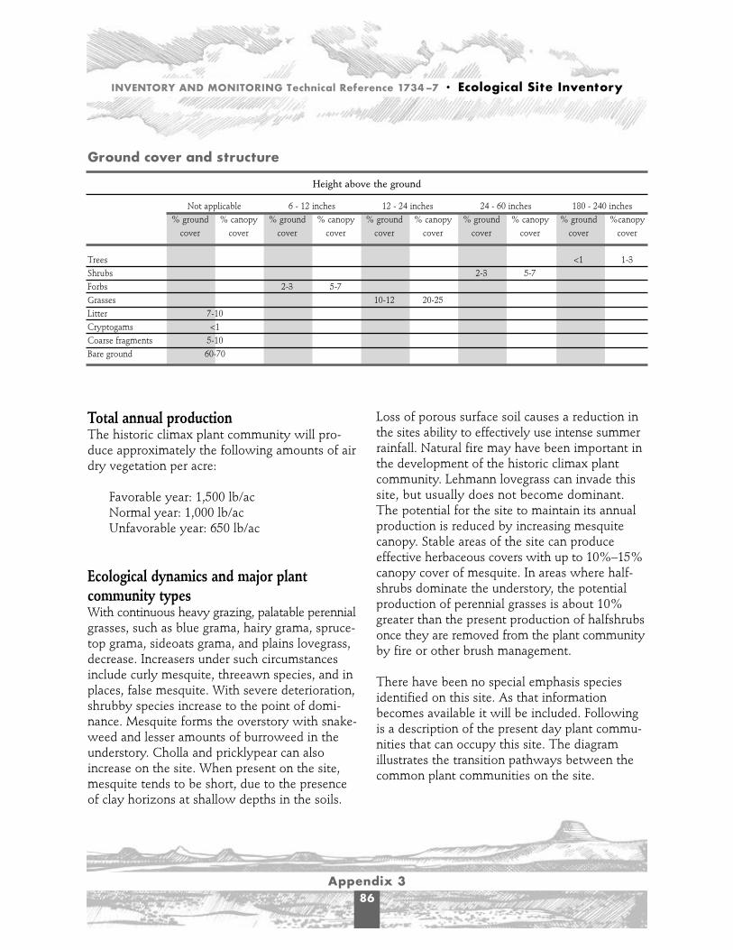
INVENTORY AND MONITORING Technical Reference 1734–7 • Ecological Site Inventory
Appendix 386
Ground cover and structure
Height above the ground
Not applicable 6 - 12 inches 12 - 24 inches 24 - 60 inches 180 - 240 inches% ground % canopy % ground % canopy % ground % canopy % ground % canopy % ground %canopy
cover cover cover cover cover cover cover cover cover cover
Trees <1 1-3Shrubs 2-3 5-7Forbs 2-3 5-7Grasses 10-12 20-25Litter 7-10Cryptogams <1Coarse fragments 5-10Bare ground 60-70
Total annual productionThe historic climax plant community will pro-duce approximately the following amounts of airdry vegetation per acre:
Favorable year: 1,500 lb/acNormal year: 1,000 lb/acUnfavorable year: 650 lb/ac
Ecological dynamics and major plantcommunity typesWith continuous heavy grazing, palatable perennialgrasses, such as blue grama, hairy grama, spruce-top grama, sideoats grama, and plains lovegrass,decrease. Increasers under such circumstancesinclude curly mesquite, threeawn species, and inplaces, false mesquite. With severe deterioration,shrubby species increase to the point of domi-nance. Mesquite forms the overstory with snake-weed and lesser amounts of burroweed in theunderstory. Cholla and pricklypear can alsoincrease on the site. When present on the site,mesquite tends to be short, due to the presenceof clay horizons at shallow depths in the soils.
Loss of porous surface soil causes a reduction inthe sites ability to effectively use intense summerrainfall. Natural fire may have been important inthe development of the historic climax plantcommunity. Lehmann lovegrass can invade thissite, but usually does not become dominant.The potential for the site to maintain its annualproduction is reduced by increasing mesquitecanopy. Stable areas of the site can produceeffective herbaceous covers with up to 10%–15%canopy cover of mesquite. In areas where half-shrubs dominate the understory, the potentialproduction of perennial grasses is about 10%greater than the present production of halfshrubsonce they are removed from the plant communityby fire or other brush management.
There have been no special emphasis speciesidentified on this site. As that informationbecomes available it will be included. Followingis a description of the present day plant commu-nities that can occupy this site. The diagramillustrates the transition pathways between thecommon plant communities on the site.
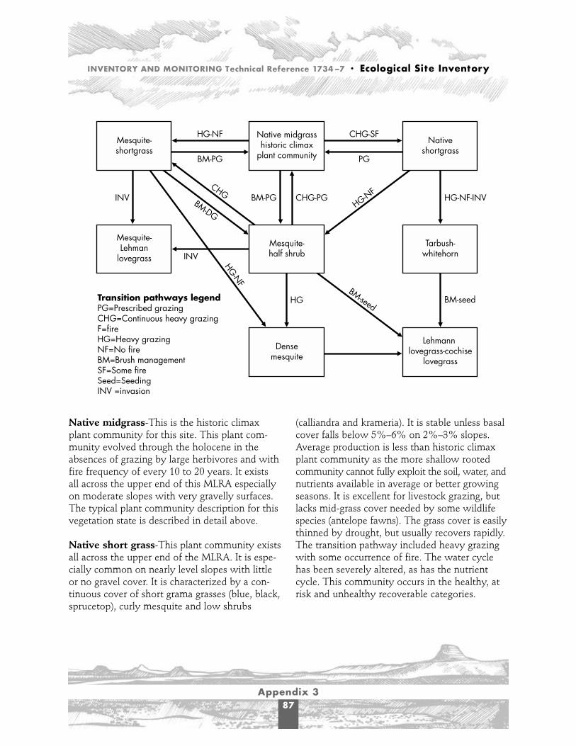
INVENTORY AND MONITORING Technical Reference 1734–7 • Ecological Site Inventory
Appendix 387
Transition pathways legendPG=Prescribed grazingCHG=Continuous heavy grazingF=fireHG=Heavy grazingNF=No fireBM=Brush managementSF=Some fireSeed=SeedingINV =invasion
Native midgrasshistoric climax
plant community
Mesquite-shortgrass
Nativeshortgrass
Mesquite-half shrub
Mesquite-Lehman
lovegrass
INV
INV
CHG-PGHG-NF
HG
BM-PG HG-NF-INV
BM-seedBM-seed
CHGBM-DG
HG-N
F
HG-NF
BM-PG
CHG-SF
PG
Tarbush-whitehorn
Densemesquite
Lehmann lovegrass-cochise
lovegrass
Native midgrass-This is the historic climaxplant community for this site. This plant com-munity evolved through the holocene in theabsences of grazing by large herbivores and withfire frequency of every 10 to 20 years. It existsall across the upper end of this MLRA especiallyon moderate slopes with very gravelly surfaces.The typical plant community description for thisvegetation state is described in detail above.
Native short grass-This plant community existsall across the upper end of the MLRA. It is espe-cially common on nearly level slopes with littleor no gravel cover. It is characterized by a con-tinuous cover of short grama grasses (blue, black,sprucetop), curly mesquite and low shrubs
(calliandra and krameria). It is stable unless basalcover falls below 5%–6% on 2%–3% slopes.Average production is less than historic climaxplant community as the more shallow rootedcommunity cannot fully exploit the soil, water, andnutrients available in average or better growingseasons. It is excellent for livestock grazing, butlacks mid-grass cover needed by some wildlifespecies (antelope fawns). The grass cover is easilythinned by drought, but usually recovers rapidly.The transition pathway included heavy grazingwith some occurrence of fire. The water cyclehas been severely altered, as has the nutrientcycle. This community occurs in the healthy, atrisk and unhealthy recoverable categories.

INVENTORY AND MONITORING Technical Reference 1734–7 • Ecological Site Inventory
Appendix 388
The following represents the typical plantcommunity of the vegetation state described asNative-Short Grass. Refer to the Historic climaxplant community for the plants in each plantgroup.
Plant group Pounds per acre
1 15-502 300-4003 15-505 15-1508 15-5010 15-5011 T12 T
Total annual production 630 lb/ac (normal year)
Mesquite short grass-This plant communityexists all across the MLRA. Mesquite canopyranges from 1%–10%. The understory is acontinuous cover of short grama grasses and/orcurly mesquite. It is stable unless basal cover fallsbelow 5%–6% on 2%–3% slopes. Production isalways less than the historic climax plant com-munity. Mesquite exploits the soil, water, andnutrients earlier in the spring and to a greaterdepth than the shallow rooted warm-seasongrasses. The grass cover is easily thinned bydrought and may be slow to recover due to thepresence of mesquite. It is good for livestockgrazing, but the tree cover can interfere withlivestock handling operations. The presence ofmesquite allows species, such as mule deer andjavelina, to use this site, but detract from itsvalue as antelope habitat. The transition pathwayincludes heavy grazing, no fires, and a proximityto mesquite in bottom-lands. The ecologicalprocesses of water cycle, nutrient cycle, andenergy flow have been severely altered. Thehydrologic functioning of this site has been
altered. This site occurs most often as at risk andunhealthy recoverable categories.
The following represents the typical plantcommunity of the vegetation state described asMesquite-Short Grass. Refer to the Historicclimax plant community for the plants in eachplant group.
Plant group Pounds per acre
1 15-502 300-4003 15-505 15-1008 15-5010 15-5012 15-150
Total annual production 665 lb/ac (normal year)
Mesquite halfshrub/cacti-This plant communityexists all across the lower and mid portion of theMLRA. Mesquite canopy ranges from 1%–10%.The understory is a diverse mixture of cacti,burroweed, broom snakeweed, and other shrubs.Perennial grasses exist in trace amounts only. Theplant community is poor for livestock grazing,poor for some wildlife species (e.g. pronghornantelope and scaled quail) and good for otherwildlife species (e.g., mule deer, javelina, andgambel quail). Transition pathway is frommesquite short grass with continued heavygrazing and the absence of fire. Almost all theecological processes on this site have beenseverely altered, and the site has lost some of therecovery mechanisms. In general, the site is notstable in this plant community and occurs mostoften as unhealthy recoverable category.
The following represents the typical plantcommunity of the vegetation state described as

INVENTORY AND MONITORING Technical Reference 1734–7 • Ecological Site Inventory
Appendix 389
Mesquite-Shrub-Cacti. Refer to the Historicclimax plant community for the plants in eachplant group.
Plant group Pounds per acre
2 15-503 15-1004 15-507 15-5011 15-15012 500-600
Total annual production 750 lb/ac (normal year)
Dense mesquite-This plant community occursall across the MLRA in small areas, especiallyhistoric heavy use areas, such as old homesteads,in horse pastures, along streams with perennialflow and other old watering locations, and alsoon archaeological sites. Mesquite canopy rangesfrom 10%–30%. The understory consists ofscattered low shrubs, remnant perennial grasses,and annual species. This plant community isvery poor for livestock grazing and poor qualityhabitat for most wildlife species. However,under the present hunting pressure in southernArizona, the oldest and largest mule deer bucksuse these mesquite thickets as hiding and escapecover. The site in this plant community is notstable. Often times so much of the soil surfacehas been lost under this condition that the sitewill not respond to treatment and the site poten-tial has been lost. In some cases the erosion hasso damaged the site that even the existingmesquite trees have difficulty surviving.Transition pathway is from mesquite short grass
with excessive grazing and no fires. This siteoccurs most as unhealthy recoverable andunhealthy unrecoverable categories.
The following represents the typical plantcommunity of the vegetation state described asDense Mesquite. Refer to the Historic climaxplant community for the plants in each plantgroup.
Plant group Pounds per acre
3 15-504 15-5012 500-600
Total annual production 620 lb/ac (normal year)
Tarbush/Whitethorn-This plant communityoccurs throughout the eastern portion of theMLRA in areas where loamy upland is adjacentto limy sites that naturally support tarbush andwhitethorn. Canopy cover of the two shrubbyspecies usually exceeds 10%. The understoryconsists of scattered low shrubs, remnant peren-nial grasses and annuals. This plant community isvery poor for livestock grazing and poor qualityhabitat for most wildlife species. The site underthis plant community is not stable. Often somuch surface soil has been lost that the site willnot respond to treatment and the site potentialhas been lost. Transition pathway is from nativemid-grass with heavy grazing, no fires, and aproximity to tarbush/whitethorn on adjacent limysites. This site occurs most as unhealthy recoverableand unhealthy unrecoverable categories.

INVENTORY AND MONITORING Technical Reference 1734–7 • Ecological Site Inventory
Appendix 390
The following represents the typical plantcommunity of the vegetation state described asTarbush-Whitethorn. Refer to the Historicclimax plant community for the plants in eachplant group.
Plant group Pounds per acre
1 15-502 15-503 15-1004 15-1008 15-5010 15-5012 500-600
Total annual production 800 lb/ac (normal year)
Mesquite-Lehmann lovegrass-This plant com-munity occurs throughout the MLRA. In nearlyall cases it has developed from mesquite nativegrasslands in the last 30 years. Livestock grazing,fire, and drought have all been demonstrated toenhance this invasion of loamy upland sitewherever there is a seed source of Lehmannlovegrass. This plant community offers a greatdeal of stability to the site. Mesquite canopy isusually less than 10%. Lehmann productionequals or exceeds native grass production.Species diversity is usually greatly reduced onthis site once Lehmann lovegrass has becomedominant. Under mesquite native grass condi-tions it is common to find 40 to 50 perennialplant species on this site. Under Lehmann domi-nance that figure will be 20 to 30 species. Thisplant community is good for livestock grazing. Itis fair for some species of wildlife (mule deer andgambel quail). It is good for small herbivores(rabbits and mice) and generally poor for manyother species, such as pronghorn antelope andscaled quail. Transition pathway is frommesquite short grass with heavy grazing, some
fires, and a Lehmann lovegrass seed source.The ecological processes on this site have beenaltered somewhat, and this site occurs ashealthy, at risk, and unhealthy recoverablecategories.
The following represents the typical plantcommunity of the vegetation state described asMesquite-Lovegrass. Refer to the Historicclimax plant community for the plants in eachplant group.
Plant group Pounds per acre
2 15-508 15-5010 15-5012 50-15013 1,200-1,400 (consists
of introduced lovegrasses,
such as Lehmann, Cochise,
Boer, and Wilman)
Total annual production 1,425 lb/ac (normal year)
Lehmann lovegrass and/or Cochise lovegrass-This plant community occurs throughout theMLRA. It exists where mechanical brush man-agement was used to control mesquite, tarbush,whitethorn, and cacti, and where lovegrassspecies were seeded. This plant communityoffers a great deal of stability to the site. Becauseof the nature of the grass species and themechanical roughening of the soil surface, thesecommunities generally produce 20–50% morethan native grass communities. Although plantspecies diversity is low in these lovegrass com-munities, it is usually better than in the woodydominated plant community it replaced. Thiscommunity is good to very good for livestockgrazing, fair for some wildlife species pronghornantelope and scaled quail), good for other species
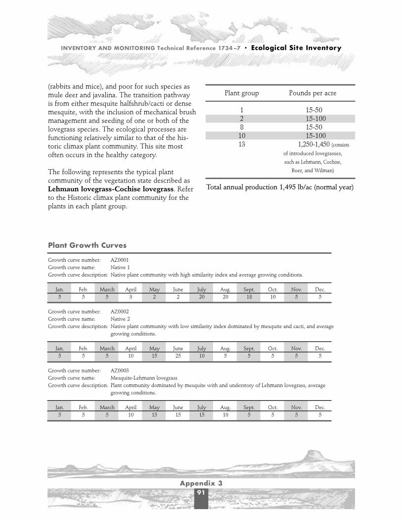
INVENTORY AND MONITORING Technical Reference 1734–7 • Ecological Site Inventory
Appendix 391
(rabbits and mice), and poor for such species asmule deer and javalina. The transition pathwayis from either mesquite halfshrub/cacti or densemesquite, with the inclusion of mechanical brushmanagement and seeding of one or both of thelovegrass species. The ecological processes arefunctioning relatively similar to that of the his-toric climax plant community. This site mostoften occurs in the healthy category.
The following represents the typical plantcommunity of the vegetation state described asLehmaun lovegrass-Cochise lovegrass. Referto the Historic climax plant community for theplants in each plant group.
Plant group Pounds per acre
1 15-502 15-1008 15-5010 15-10013 1,250-1,450 (consists
of introduced lovegrasses,
such as Lehmann, Cochise,
Boer, and Wilman)
Total annual production 1,495 lb/ac (normal year)
Plant Growth Curves
Growth curve number: AZ0001Growth curve name: Native 1Growth curve description: Native plant community with high similarity index and average growing conditions.
Jan. Feb. March April May June July Aug. Sept. Oct. Nov. Dec.5 5 5 3 2 2 20 20 18 10 5 5
Growth curve number: AZ0002Growth curve name: Native 2Growth curve description: Native plant community with low similarity index dominated by mesquite and cacti, and average
growing conditions.
Jan. Feb. March April May June July Aug. Sept. Oct. Nov. Dec.5 5 5 10 15 25 10 5 5 5 5 5
Growth curve number: AZ0003Growth curve name: Mesquite-Lehmann lovegrassGrowth curve description: Plant community dominated by mesquite with and understory of Lehmann lovegrass, average
growing conditions.
Jan. Feb. March April May June July Aug. Sept. Oct. Nov. Dec.5 5 5 10 15 15 15 10 5 5 5 5

INVENTORY AND MONITORING Technical Reference 1734–7 • Ecological Site Inventory
Appendix 392
Animal communityThe plant community on this site is well suitedto grazing by both domestic livestock of all kindsand by wildlife at all seasons of the year.Currently the majority of the livestock use onthis site is with mother cows in a cow-calf oper-ation. Historic use has always been a cow/calftype operation, but there have been periods oflarge numbers of stocker cattle on these ranges.Sheep use has been slight historically. The mainproblem to the use and management of livestockon this site is the lack of natural water sources.
This site is important for many wildlife species.Major species include desert mule deer, pronghornantelope, gambels quail, scaled quail, and black-tailed jackrabbit. Water developments are veryimportant to these and other wildlife on this site.Being an open grassland, this site is also home toa variety of small herbivores, birds, and theirassociated predators. With the exception ofpronghorn antelope, this site is mainly a foragearea for larger wildlife species. The value of thissite for food or cover requirements for specificwildlife species changes with the changes in thevegetation that occur from one plant communityto another. Each plant community and each animalspecies must be considered individually. Generalinformation has been included here and in theecological dynamic section of this site description.
Associated site-This site is associated with theLimy Upland 12-16 PZ and the Loamy Bottom sites.
Similar sites-With the historic climax plantcommunity, this site is not similar enough to anyother site to cause a problem or concern. As thissite deteriorates it may easily be confused withother deteriorated sites, such as Limy Upland.Many sites will deteriorate into very similarplant communities.
Site DocumentationAuthor: Original WHN 1976
Revised DGR 1987
Supporting data for site development-The his-toric climax plant community has been determinedby study of rangeland relict areas or areas protectedfrom excessive grazing. Trends in plant communitiesgoing from heavily grazed areas to lightly grazedareas, seasonal use pastures, and historical accountshave also been used. The following transect andclipping data also documents this site. There are 21permanent transect locations on this site.
Sampling technique EC GC FC PCSCS-Range 417 10 15 15 3SCS AZ-Range-1 1 7 10 13
Type locality:Pima Co Buenos Aires NWR, Sec. 19,
T21S, R8ECochise Co. Oak Ranch, Sec.2, T18S, R28ECochise Co. Ft. Huachuca, Sec.17, T21S,
R19E unsurveyedSanta Cruz Co. Santa Fe Ranch, Sec. 13, T23S, R14EPinal Co. Tom Mix Hwy ROW, Sec.2,
T10S, R13E
Field offices:Casa Grande ChandlerDouglas PhoenixSafford San CarlosSells TucsonWillcox
Relationship to other established classifications-This site would most closely fit A.W. Kuckler’sPotential Natural Vegetation as unit number 58Grama - Tobosa - Shrubsteepe. It most closely fits theSociety for Range Management’s Rangeland CoverTypes as unit number 505 Grama - Tobosa Shrub.

INVENTORY AND MONITORING Technical Reference 1734–7 • Ecological Site Inventory
Appendix 393
Plant species index-(This section provides across reference for common names, scientificnames, and national symbol. It will be generatedby ESIS, no input required here.)
Other references (list other references used inthe description or correlation of this site.)
Site approval-This site has been reviewed andapproved for use.
State Rangeland Management Specialist
Date
Ecological site interpretationsGrazingThe plant community on this site is suitable forgrazing by all classes of livestock at any season.With thin, course textured surfaces, and over
argillic horizons, these soils become less effectivein catching summer rainfall if the grass cover isdisturbed or depleted. With a good grass cover,the clayey subsoil releases moisture slowly tothe plants over the summer season. Lehmannlovegrass can invade this site slowly, but seldomforms a monotype. At the first sign of invasion,proper use of the native perennials must bepracticed to avoid letting lovegrass spread.Herbaceous forage is deficient in protein in thewinter. This site has no natural surface waterassociated with it; therefore, water developmentfor livestock is necessary for utilization of thissite.
Initial starting stocking rates will be determinedwith the landowner or decision maker. Theywill be based on past use histories and type andcondition of the vegetation. Calculations used todetermine an initial starting stocking rate will bebased on forage preference ratings.
Forage preferences by season for cattle(P = preferred, D = desirable, U = undesirable)
Plant species Dec/Feb March/May June/Aug Sept/Nov
Sideoats grama U P P P.Plains lovegrass U P P PCane beardgrass U D P DBlue grama D P P PSprucetop grama D P P PCurly mesquite D P P PHarry grama D P P PSpidergrass U U D URed threeawn U D U UPerennial forbs P P P PFalse mesquite U P D PRatany species P P D PZinnia species P P D PMesquite U (leaves) P (new leaves) P (beans) P (beans)Staghorn cholla (fruits) P D P PPricklypear (fruits) U U P P
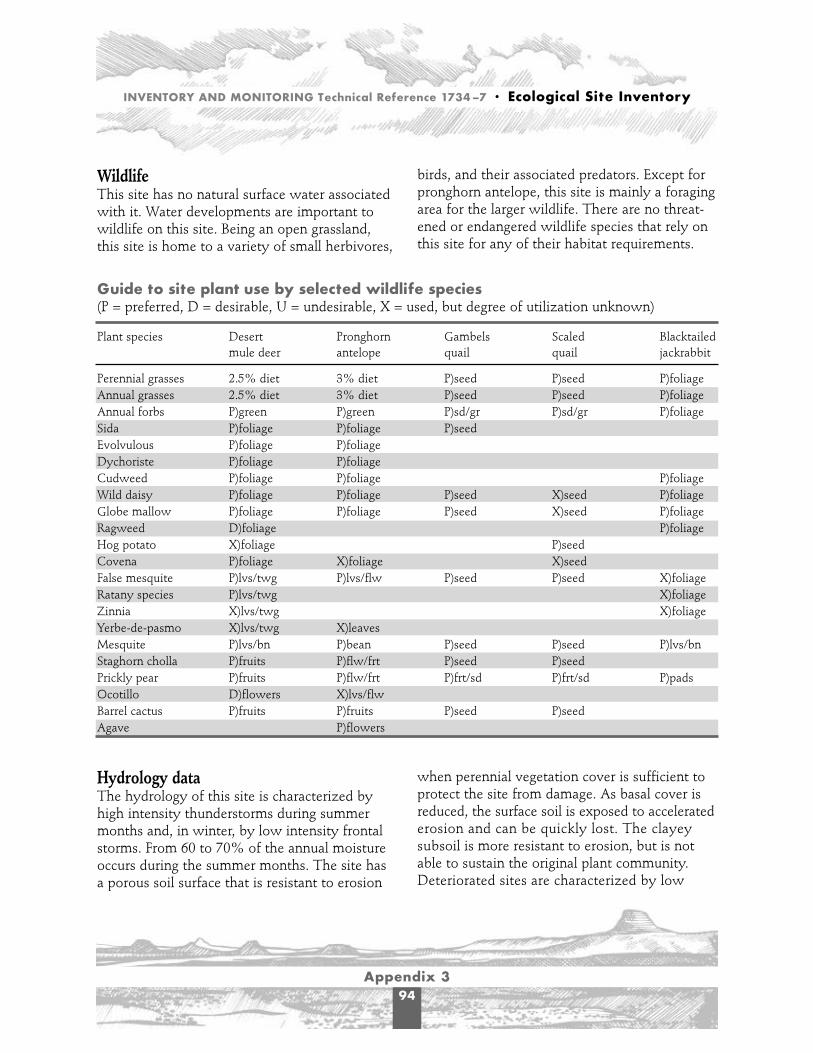
INVENTORY AND MONITORING Technical Reference 1734–7 • Ecological Site Inventory
Appendix 394
WildlifeThis site has no natural surface water associatedwith it. Water developments are important towildlife on this site. Being an open grassland,this site is home to a variety of small herbivores,
birds, and their associated predators. Except forpronghorn antelope, this site is mainly a foragingarea for the larger wildlife. There are no threat-ened or endangered wildlife species that rely onthis site for any of their habitat requirements.
Hydrology dataThe hydrology of this site is characterized byhigh intensity thunderstorms during summermonths and, in winter, by low intensity frontalstorms. From 60 to 70% of the annual moistureoccurs during the summer months. The site hasa porous soil surface that is resistant to erosion
when perennial vegetation cover is sufficient toprotect the site from damage. As basal cover isreduced, the surface soil is exposed to acceleratederosion and can be quickly lost. The clayeysubsoil is more resistant to erosion, but is notable to sustain the original plant community.Deteriorated sites are characterized by low
Guide to site plant use by selected wildlife species(P = preferred, D = desirable, U = undesirable, X = used, but degree of utilization unknown)
Plant species Desert Pronghorn Gambels Scaled Blacktailed mule deer antelope quail quail jackrabbit
Perennial grasses 2.5% diet 3% diet P)seed P)seed P)foliageAnnual grasses 2.5% diet 3% diet P)seed P)seed P)foliageAnnual forbs P)green P)green P)sd/gr P)sd/gr P)foliageSida P)foliage P)foliage P)seedEvolvulous P)foliage P)foliageDychoriste P)foliage P)foliageCudweed P)foliage P)foliage P)foliageWild daisy P)foliage P)foliage P)seed X)seed P)foliageGlobe mallow P)foliage P)foliage P)seed X)seed P)foliageRagweed D)foliage P)foliageHog potato X)foliage P)seedCovena P)foliage X)foliage X)seedFalse mesquite P)lvs/twg P)lvs/flw P)seed P)seed X)foliageRatany species P)lvs/twg X)foliageZinnia X)lvs/twg X)foliageYerbe-de-pasmo X)lvs/twg X)leavesMesquite P)lvs/bn P)bean P)seed P)seed P)lvs/bnStaghorn cholla P)fruits P)flw/frt P)seed P)seedPrickly pear P)fruits P)flw/frt P)frt/sd P)frt/sd P)padsOcotillo D)flowers X)lvs/flwBarrel cactus P)fruits P)fruits P)seed P)seedAgave P)flowers

INVENTORY AND MONITORING Technical Reference 1734–7 • Ecological Site Inventory
Appendix 395
infiltration and excessive runoff. This site natu-rally delivers water to adjacent sites downstreamby overland flow. Concentrated flow patterns arecommon and can easily become rills and gulliesif cover is lost.
Wood productsConsiderable amounts of mesquite occupy sever-al present day plant communities. Wood prod-ucts potential is low on this site. Mesquitesremain small and shrubby because of the soils.


Ap
pe
nd
ix 4
97
Appendix 4 - Vegetation Production WorksheetInventory Code _______ Management Unit or Allotment __________________________ Elevation _______ % slope _______ Slope Aspect _______ Landform _______
Site Write-up Area Number _______ Ecological Site Number _________________ Ecological Site Name _____________________ Ecological Condition ____________
Transect No. _______ % SWA _______ Soil Map Unit No. _______ Soil Taxon Name _____________________ Soil Phase Texture Class _______ Soil Phase Texture Modifier
Date ____________ Recorder ____________ Pasture Number ____________ Estimate Total Production _________________ (lb/ac) Vegetation Type_______________
Stratum No. _______ Sampled? (circle) Yes No
Estimated Weight Units by Species (2) Adjustments Double SamplingPlant Plant Species Total Wt Wt Plot Plot Adw Util Gwth Clip Clip Clip/ TotalSpecies Common Wt Unit Meas Size Size Adj Adj Adj Plots Plots Est WeightSymbol Name Units Wt gm/lb CF Est Clip CF LB/AC
Wt Wt
(1) (Optional) P-1 P-2 P-3 P-4 P-5 P-6 P-7 P-8 P-9 P-10 (3) (4) (5) (6) (7) (8) (9) (10) (11) (12) (13) (14)
REMARKS:

INVENTORY AND MONITORING Technical Reference 1734–7 • Ecological Site Inventory
Appendix 498
Instructions for Filling out the Vegetation Production WorksheetBe sure to complete the top portion of the worksheet. The following items deal with the vegetation portion of the transect.
Column 1 Enter the acceptable plant symbol from the USDA PLANTS Database at http://plants.usda.gov/. You can even download alist of species specific for your State. Entering the common name of the plant species is optional.
Column 2 For plots 1 through 10 (P-1 through P-10), enter an estimate of the number of weight units by species occurring in theappropriate plot(s), or the estimated weight by species occurring in the plots. The weight unit number can be expressednumerically (e.g. 6, 11.5). If weight by species is recorded, the number entered would be the total estimated weight forthat species. For example, a number of 52 in P-3 would mean that 52 grams or pounds is the estimated weight for thatspecies in plot 3.
Note: When double sampling is used to determine a correction factor, circle the plot numbers that are clipped.
Column 3 This column represents the summarized total number of weight units or weight by species occurring in plots 1 through10 as estimated by the data collector.
Column 4 If weight units are entered in the plot data (2) columns, complete this column by entering the weight unit weight byspecies used by the data collector. If weight by species was entered in the plot data (2) columns, rather than weightunits, enter 1 in this column.
Column 5 Enter the weight measure unit (grams or pounds) for the weight unit weight shown in column 4 or the summarizedspecies weight listed in column 3.
Column 6 Enter the plot size used to estimate weight units or weight by species (e.g., plot sizes 9.6 ft2, 96 ft2, or .01 acre).
Column 7 Enter the plot size conversion factor (CF) from Tables 6 or 7 in Chapter 4.
Column 8 Enter the appropriate ADW percent in decimal form, from green weight conversions tables, Appendix 7 (Percent Air-DryWeight Conversion Table), or local conversion tables.
Column 9 Complete this column only when the current season’s growth of plant species has been removed by grazing. Enter theamount in decimal form (e.g., 0.25, 0.40, 0.60), which best reflects the percentage of the “plant remaining” after grazingutilization has occurred. For example, if a plant species averages 30 percent utilization in the production transect, thepercentage of plant material remaining would be 70 percent. Thus, the adjustment entered for that particular specieswould be .70. Utilization may vary through the plots, requiring an estimate of the average use.
Column 10 Enter the cumulative percent of growth, in decimal form, that has occurred up to the time plot data is collected. Thevalues entered can reflect the growth curves for the site (as listed in some site descriptions) or be based upon locallydeveloped growth curve data for each species.
When doubling sampling is used to determine a correction factor, data will be recorded in columns 11 through 13; otherwise, thesecolumns will be left blank.
Column 11 For each plant species occurring in the clipped plots, enter the total estimated weight (to nearest gram or pound) bymultiplying the total weight units by the weight unit weight for all clipped plots.
Column 12 For each plant species occurring in the clipped plots, enter the total clipped (harvested) weight (to nearest gram orpound) for all clipped plots.
Column 13 To determine the correction factor, divide column (12) by column (11) for each species and enter to the nearest hundredth.A factor of 1 indicates the estimates are the same as the clipped weights. A factor below one 1 indicates estimates arehigh. A factor above 1 indicates estimates are low.
Total pounds per acre production result:
Column 14 This column represents the air-dry reconstructed weight in pounds per acre after considering all conversion, correction,and adjustment factors. Calculate pounds per acre (nearest pound) for each plant species by multiplying the number ofweight units (3), times the weight of the individual weight unit (4), times the plot size conversion factor (7), times theADW adjustment (8), times the clipped conversion factor (13). Divide by the utilization adjustment (9), times the growthadjustment (10). The formula is:
Pounds per Acre = Columns (3) x (4) x (7) x (8) x (13)Columns (9) x (10)

INVENTORY AND MONITORING Technical Reference 1734–7 • Ecological Site Inventory
Appendix 599
Appendix 5 - Foliage DensenessClasses Utah JuniperGuide for Determining Current Yield of Utah Juniper in Utah Upland Stony Loam (Juniper) Site
Current Yield Air Dry PoundsCrown Weight 10 50 100 200 300 400 500diameter per tree trees trees trees trees trees trees trees
Sparse foliage1 0.1 1 5 10 20 30 40 502 0.3 3 15 30 60 90 120 1503 0.6 6 30 60 120 180 240 3004 1.0 10 50 100 200 300 400 5005 1.3 13 65 130 260 390 520 6506 1.6 16 80 160 320 480 640 8007 1.9 19 95 190 380 570 760 9508 2.3 23 115 230 460 690 920 11509 2.6 26 130 260 520 780 1040 130010 2.9 29 145 290 580 870 1160 145011 3.3 33 165 330 660 990 1320 165012 3.6 36 180 360 720 1080 1440 180013 4.0 40 200 400 800 1200 1600 200014 4.4 44 220 440 880 1320 1760 220015 4.7 47 235 470 940 1410 1880 235016 5.1 51 255 510 1020 1530 2040 255017 5.5 55 275 550 1100 1650 220018 5.8 58 290 580 1160 1740 232019 6.2 62 310 620 1240 1860 248020 6.6 66 330 660 1320 1980 2640
Medium foliage1 0.1 1 5 10 20 30 40 502 0.3 3 15 30 60 90 120 1503 0.6 6 30 60 120 180 240 3004 1.0 10 50 100 200 300 400 5005 1.4 14 70 140 280 420 560 7006 1.9 19 95 190 380 570 760 9507 2.5 25 125 250 500 750 1000 12508 3.1 31 155 310 620 930 1240 15509 3.8 38 190 380 760 1140 1520 190010 4.6 46 230 460 920 1380 1840 230011 5.4 54 270 540 1080 1620 2160 270012 6.2 62 310 620 1240 1860 248013 7.2 72 360 720 1440 216014 8.1 81 405 810 1620 243015 9.1 91 455 910 1820 273016 10.2 102 510 1020 204017 11.3 113 565 1130 226018 12.4 124 620 1240 248019 13.6 136 680 136020 14.8 148 740 1480

INVENTORY AND MONITORING Technical Reference 1734–7 • Ecological Site Inventory
Appendix 5100
Guide for Determining Current Yield of Utah Juniper (continued)
Current Yield Air Dry PoundsCrown Weight 10 50 100 200 300 400 500diameter per tree trees trees trees trees trees trees trees
Dense foliage1 0.1 1 5 10 20 30 40 502 0.3 3 15 30 60 90 120 1503 0.7 7 35 70 140 210 280 3504 1.2 12 60 120 240 360 480 6005 1.9 19 95 190 380 570 760 9506 2.7 27 135 270 540 810 1080 13507 3.6 36 180 360 720 1080 1440 18008 4.7 47 235 470 940 1410 1880 23509 5.9 59 295 590 1180 1770 236010 7.2 72 360 720 1440 216011 8.6 86 430 860 1720 258012 10.2 102 510 1020 204013 11.9 119 595 1190 238014 13.7 137 685 1370 274015 15.6 156 780 156016 17.7 177 885 177017 19.9 199 995 199018 22.2 222 1110 222019 24.6 246 1230 246020 27.2 272 1360 2720

INVENTORY AND MONITORING Technical Reference 1734–7 • Ecological Site Inventory
Appendix 6101
Appendix 6 - Examples ofWeight Units
(Reprinted from 190-vi, NRPH, September 1977)


INVENTORY AND MONITORING Technical Reference 1734–7 • Ecological Site Inventory
Appendix 7103
Appendix 7 - Percentage Air-dryWeight Conversion TablePercentage of Air-dry Weight in Harvested Plant Material at Various Stages of Growth
Before heading Headed out: Seed ripe: Leaves dry ApparentGrasses initial growth to boot stage leaf tips stems dormancy
boot stage to flowering drying partly dry(%) (%) (%) (%) (%)
Cool season 35 45 60 85 95wheatgrassesperennial bromesbluegrassesprairie junegrass
Warm season 30 45 60 85 95Tall grasses
bluestemsindiangrassswitchgrass
Midgrasses 40 55 65 90 95side-oats gramatabosagalleta
Short grasses 45 60 80 90 95blue gramabuffalograssshort three-awns
New leaf and Older and Green DryTrees twig growth full size fruit fruit
until leaves greenare full size leaves
(%) (%) (%) (%)
Evergreen conifers 45 55 35 85ponderosa pine, slashpine-longleaf pineUtah juniperrocky mountain juniperspruce
Live oak 40 55 40 85
Deciduous 40 50 35 85blackjack oakpost oakhickory
USDA, National Resources Conservation Service, National Range and Pasture Handbook

INVENTORY AND MONITORING Technical Reference 1734–7 • Ecological Site Inventory
Appendix 7104
Percentage of air dry matter (continued)
New leaf and Older and Green GreenShrubs twig growth until full-size fruit fruit
leaves are full size green leaves(%) (%) (%) (%)
Evergreen 55 65 35 85big sagebrushbitterbrushephedraalgeritagallberry
Deciduous 35 50 30 85snowberryrabbitbrushsnakeweedGambel oakmesquite
Yucca and yuccca like plants 55 65 35 85yuccasotolsaw-palmetto
Initial growth Flowering to Seed ripe Leaves dry DryForbs to flowering seed maturity leaf tips dry stems drying
(%) (%) (%) (%) (%)
Succulent 15 35 60 90 100violetwaterleafbuttercupbluebellsonion, lilies
Leafy 20 40 60 90 100Lupinelespedezacompassplantbalsamroottickclover
Fibrous leavesor mat 30 50 75 90 100phlox, mat eriogonumpussytoes
Succulents New growth pads and fruit Older pads Old growth in dry years(%) (%) (%)
Prickly pear and barrel cactus 10 10 15+Cholla cactus 20 25 30+

INVENTORY AND MONITORING Technical Reference 1734–7 • Ecological Site Inventory
Appendix 8105
Type Subtype CodeSand Sage 4046Chamise 4051Manzanita 4052Ceanothus 4053Shinnery Oak 4054Chaparral 4055Mountain Mahogany 4056Bitterbrush 4057Oakbrush 4058Serviceberry 4059Mountain shrub 4060Blackbrush 4061Cactus 4062Joshua Tree 4063Yucca 4064White Thorn 4065Paloverde Cerci 4066Bursage FRDE-FRD 4067Catclaw 4068Sotol 4069Mariola 4070Snakeweed 4071Fringed Sagebrush 4072Clubmoss 4073Willow 4074Turpentine Brush 4075Burroweed HATE 4076Mormon Tea 4077Skunk Bush 4078Ocotilla 4079Sacahuiste 4080Alder 4081Snowberry 4082Other Shrub 4999
Appendix 8 - Vegetation Types andSubtypesInformation ResourceManagement (IRM) Codes forVegetation Types and SubtypesType Subtype CodeAnnual Forbs 0000
Filaree 0001Halogeton 0002Other Forbs 0999
Grass 1000Short Grass 1001Mid Grass 1002 Tall Grass 1003 Crested Wheat Grass 1004Mixed Grass Seeding 1005Other Grass 1999
Grasslike Sedge 2001Rush 2002Other Grasslike 2999
Perennial Forbs 3001Shrub 4000
Black Greasewood 4001Bailey Greasewood 4002Creosote Bush 4011Tarbush 4012 Broom Dalea 4013Winterfat 4015Mesquite 4021Shadscale 4031Nuttal Saltbush 4032Mat Saltbush 4033Fourwing Saltbush 4034Other Saltbush 4035Desert Saltbush AT 4036Mixed Desert Shrub 4037Big Sagebrush 4041Low Sagebrush 4042Black Sagebrush 4043Other Sagebrush 4044Rabbitbrush 4045
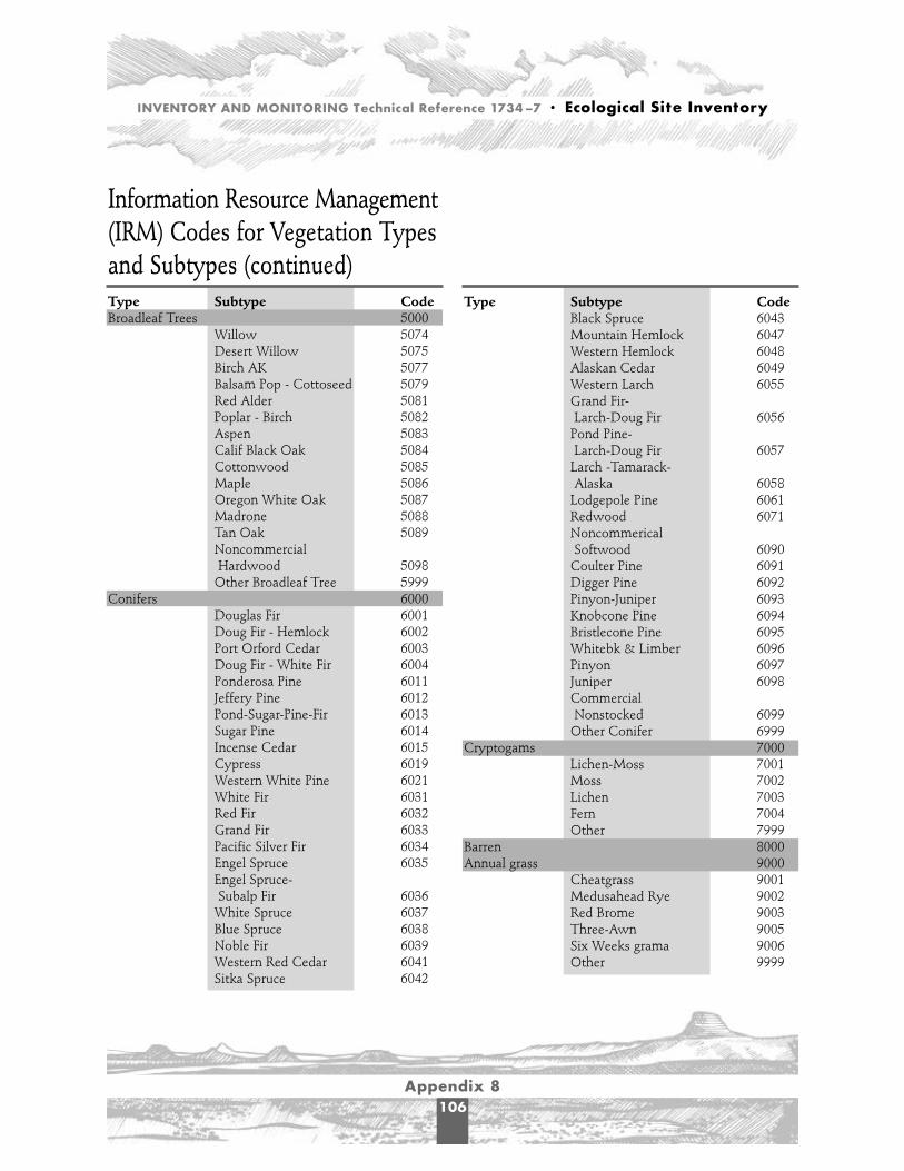
INVENTORY AND MONITORING Technical Reference 1734–7 • Ecological Site Inventory
Appendix 8106
Information Resource Management(IRM) Codes for Vegetation Typesand Subtypes (continued)Type Subtype CodeBroadleaf Trees 5000
Willow 5074Desert Willow 5075Birch AK 5077Balsam Pop - Cottoseed 5079Red Alder 5081Poplar - Birch 5082Aspen 5083Calif Black Oak 5084Cottonwood 5085Maple 5086Oregon White Oak 5087Madrone 5088Tan Oak 5089NoncommercialHardwood 5098
Other Broadleaf Tree 5999Conifers 6000
Douglas Fir 6001Doug Fir - Hemlock 6002Port Orford Cedar 6003Doug Fir - White Fir 6004Ponderosa Pine 6011Jeffery Pine 6012 Pond-Sugar-Pine-Fir 6013Sugar Pine 6014 Incense Cedar 6015 Cypress 6019Western White Pine 6021White Fir 6031Red Fir 6032Grand Fir 6033Pacific Silver Fir 6034Engel Spruce 6035Engel Spruce-Subalp Fir 6036
White Spruce 6037Blue Spruce 6038Noble Fir 6039Western Red Cedar 6041Sitka Spruce 6042
Type Subtype CodeBlack Spruce 6043Mountain Hemlock 6047Western Hemlock 6048Alaskan Cedar 6049Western Larch 6055Grand Fir-Larch-Doug Fir 6056
Pond Pine-Larch-Doug Fir 6057
Larch -Tamarack-Alaska 6058
Lodgepole Pine 6061Redwood 6071Noncommerical Softwood 6090
Coulter Pine 6091Digger Pine 6092Pinyon-Juniper 6093Knobcone Pine 6094Bristlecone Pine 6095Whitebk & Limber 6096Pinyon 6097Juniper 6098CommercialNonstocked 6099
Other Conifer 6999Cryptogams 7000
Lichen-Moss 7001Moss 7002Lichen 7003Fern 7004 Other 7999
Barren 8000Annual grass 9000
Cheatgrass 9001Medusahead Rye 9002Red Brome 9003Three-Awn 9005Six Weeks grama 9006Other 9999

INVENTORY AND MONITORING Technical Reference 1734–7 • Ecological Site Inventory
Appendix 9107
Appendix 9 - Similarity Index Form Management Unit or Allotment Examiner Ecological Site Location Reference Plant Community Date
A B C D EPlant Species Name Production/acres in Annual production PoundsGroup reference plant community in lb/acre (actual or allowable
(from ecological site reconstructeddescription)
TOTALS
SIMILARITY INDEX to Native Midgrass Community = (Total of E divided by total of C)


INVENTORY AND MONITORING Technical Reference 1734–7 • Ecological Site Inventory
Appendix 10109
Appendix 10 - Data Element CodesA complete listing of all data elements can be found in the Corporate Data Dictionary at:http://sc2962.sc.blm.gov/datashopper/default.asp
Data Element Landform 5132
Code Landform Name Description
ALF ALLUVIAL FAN The fan like deposit of a steam where it issues from a gorge upon a plain.
ARY ARROYO
BAL BADLANDS An area characterized by the intricate and sharp erosional sculpture of generallyweak rocks forming nearly horizontal beds.
BNC BENCH Level narrow platform breaking up slope
BTT BUTTE An isolated hill or small mountain with steep sides. With a smaller summitarea than a mesa.
CAN CANYON A deep narrow valley with precipitous sides where downward cutting of thestream greatly exceeds weathering.
CHL CHANNEL The bed of a single or braided watercourse that is commonly barren ofvegetation.
CIN CINDER CONE
CRT CREST The very narrow commonly linear top of an erosional ridge, hill, mountain.
DMR DRY MEADOW RIPARIAN
FAN FAN PIEDMONT The most extensive major landform of most piedmont slopes, formed by thelateral coalescense of mountain-front alluvial fans downslope into one generallysmooth slope without the transverse undulations of the semi-conical alluvialfans by accretion of fans aprons.
FPL FLOOD PLAIN A flat surface that may be submerged by waterflow built up by stream deposition.
GUL GULLY Gullies, arroyos, wadis, and gulches.
HBK HOGBACK A ridge of land formed by the outcropping edges of tilted strata; a ridge witha sharp summit and steeply sloping sides.
ISR INTERMITTENT STREAM

INVENTORY AND MONITORING Technical Reference 1734–7 • Ecological Site Inventory
Appendix 10110
Code Landform Name Description
ITB INTERMONTANE BASIN A relatively small structural depression within a mountain range that is partlyfilled with alluviam and commonly drains externally through a narrower mountain valley.
MAN LAVA FLOW- NONVEGETATED
MAV LAVA FLOW- VEGETATED
MSA MESA An isolated hill or mountain having abrupt or steeply sloping sides and a level top.
MTN MOUNTAIN A steep elevation with a restricted summit area projecting 1000 feet or more above the surrounding land surface.
OLR LAKE RIPARIAN
ORR RESERVOIR RIPARIAN
OSR STREAM RIPARIAN
PED PEDIMENT A broad, gently sloping bedrock surface with low relief that is situated at thefoot of a much steeper mountain slope.
PYA PLAYA An undrained basin that becomes at times a shallow lake on which evaporationmay leave a deposit of salt.
RAV RAVINE Larger than a gully, smaller than a valley.
RDG RIDGE A range of hills or mountains or the upper part of such a range; an extendedelevation between valleys.
SDL SADDLE A ridge connecting two higher elevations; a low point in the crestline of a ridge.
SDN SAND DUNE Sand dunes and sand hills.
SRP SCARP A line of cliffs produced by faulting or erosion.
SUM SUMMIT The flattish top of a an erosional fan remnant, hill, or mountain.
SWL SWALE
TRC TERRACE A level and ordinarily rather narrow plain usually with a steep front borderinga river, a lake, or the sea.
UPL UPLANDS High land especially far from the sea; ground elevated above the lowlands along rivers.
VAL VALLEY An elongated depression of the earth’s surface commonly situated between rangesor hills or mountains and often comprising a drainage area and an area of generally flat land and drained or watered by a large river and its tributary streams.
WMR WET MEADOW- RIPARIAN

INVENTORY AND MONITORING Technical Reference 1734–7 • Ecological Site Inventory
Appendix 10111
Soil Phase - Soil Phase -Texture Class 4991 Texture Modifier data element 4992
Code Texture Class Code Texture Modifier
C CLAY BY BoulderyCL CLAY LOAM BYV Very Bouldery COS COARSE SAND BYX Extremely BoulderyCOSL COARSE SANDY LOAM CB CobblyFS FINE SAND CBA Angular CobblyFSL FINE SANDY LOAM CBV Very CobblyL LOAM CBX Extremely CobblyLCOS LOAMY COARSE SAND CN ChenneryLFS LOAMY FINE SAND CNV Very ChenneryLS LOAMY SAND CNX Extremely ChenneryLVSF LOAMY VERY FINE SAND CR ChertyS SAND CRC Coarse ChertySC SANDY CLAY CRV Very ChertySCL SANDY CLAY LOAM CRX Extremely ChertySI SILT FL FlaggySIC SILTY CLAY FLV Very FlaggySICL SILTY CLAY LOAM FLX Extremely FlaggySIL SILT LOAM GR GravellySL SANDY LOAM GRC Coarse GravellyVFS VERY FINE SAND GRF Fine GravellyVFSL VERY FINE SANDY LOAM GRV Very Gravelly
GRX Extremely GravellyMK MuckyPT peatyRB RubblySH ShalySHV Very ShalySHX Extremely ShalySR StratifiedST StonySTV Very StonySTX Extremely StonySY SlatySYV Very SlatySYX Extremely Slaty


REPORT DOCUMENTATION PAGE Form ApprovedOMB No. 0704-0188
Standard Form 298 (Rev. 2-89)Prescribed by ANSI Std. Z39-18296-102
NSN 7540-01-280-5500
Public reporting burden for this collection of information is estimated to average 1 hour per response, including the time for reviewing instructions, searching existing data sources, gathering and maintaining the data needed, and completing and reviewing the
collection of information. Send comments regarding this burden estimate or any other aspect of this collection of infromation, including suggestions for reducing this burden, to Washington Headquarters Services, Directorate for Information Operations and Reports,
1215 Jefferson Davis Highway, Suite 1204, Arlington, VA 22202-4302, and to the Office of Management and Budget, Paperwork Reduction Project (0704-0188), Washington, DC 20503.
1. AGENCY USE ONLY (Leave blank) 2. REPORT DATE 3. REPORT TYPE AND DATES COVERED
4. TITLE AND SUBTITLE 5. FUNDING NUMBERS
7. PERFORMING ORGANIZATION NAME(S) AND ADDRESS(ES) 8. PERFORMING ORGANIZATIONREPORT NUMBER
10. SPONSORING/MONITORINGAGENCY REPORT NUMBER
11. SUPPLEMENTARY NOTES
12a.DISTRIBUTION/AVAILABILITY STATEMENT 12b.DISTRIBUTION CODE
13. ABSTRACT (Maximum 200 words)
14. SUBJECT TERMS 15. NUMBER OF PAGES
16. PRICE CODE
17. SECURITY CLASSIFICATIONOF REPORT
18. SECURITY CLASSIFICATIONOF THIS PAGE
19. SECURITY CLASSIFICATIONOF ABSTRACT
20. LIMITATION OF ABSTRACT
Dec. 2001 Final
Inventory and Monitoring—Technical Reference 1734-7Ecological Site Inventory
U.S. Department of the InteriorBureau of Land ManagementNational Science and Technology CenterP.O. Box 25047Denver, CO 80225-0047
BLM/ST/ST-01/003+1734
Technical Reference 1734-7 describes the procedures for planning and conducting ecological site inventoriesand for documenting ecological site descriptions. It includes detailed information about mapping ecologicalsites and plant communities. It includes information about the collection of vegetation production data andthe use of the data for determining a similarity index. It discusses plant succession and state and transitionpathways.
vegetation production, soil map units, vegetation mapping, ecological sites, state and tran-sition pathways, site write-up area, stratification, vegetation subtypes, similarity index
Unclassified Unclassified Unclassified UL
128 including covers
6. AUTHOR(S)
Edward F. Habich
9. SPONSORING/MONITORING AGENCY NAME(S) AND ADDRESS(ES)


The mention of trade names or commercial products does not constitute endorsement or recommendation for use by the Federal Government.

U.S. Department of the InteriorBureau of Land Management