inventory part 2
DESCRIPTION
SCMTRANSCRIPT

Copyright © 2014 - Fadi Kotob
SESSION 6

Copyright © 2014 - Fadi Kotob
Chapter 12 !
Managing Inventories Part 2

Copyright © 2014 - Fadi Kotob
Adapted - Collier & Evans (2013). OM4, South-Western, Cengage Learning. ISBN-13: 978-1-133-37242-4
!
Last week, I started covering chapter 12 “Managing Inventories”. !
What do you remember from what was covered?

Copyright © 2014 - Fadi Kotob
Learning Objectives
- Explain and calculate the economic order quantity and inventory cost
- Briefly explain the importance of safety stock and service levels when managing a fixed order system when demand is uncertain
- Briefly explain the principal decisions when managing a fixed period system
- Briefly explain some of the additional types of inventory systems
- Explain the different approaches that an organisation could use to minimise the problem of inaccurate inventory

Copyright © 2014 - Fadi Kotob
Adapted - Collier & Evans (2013). OM4, South-Western, Cengage Learning. ISBN-13: 978-1-133-37242-4
It is a classic economic model developed in the early 1900s that minimises total cost, which is the sum of the inventory holding cost and the ordering cost. !
The EOQ Model
This week I will start by explaining the Economic Order Quantity (EOQ).
What is the Economic Order Quantity (EOQ)?

Copyright © 2014 - Fadi Kotob
Adapted - Collier & Evans (2013). OM4, South-Western, Cengage Learning. ISBN-13: 978-1-133-37242-4
• EOQ is based on the following assumptions:
- Only 2 types of costs are relevant: ordering/setup (S) and holding (H)
- Demand is constant
- Demand for items is independent (Only a single item (SKU) is considered)
- There is certainty in demand, lead time and supply
- The entire order quantity (Q) arrives in the inventory at one time.
- No stockouts are allowed.
The EOQ Model Assumptions
FROM THESE ASSUMPTIONS, LET’S MOVE TO LEARN HOW TO CALCULATE EOQ & THE ANNUAL INVENTORY COST

© 2 0 1 3 O M 4 C e n g a g e L e a r n i n g . A l l R i g h t s R e s e r v e d . M a y n o t b e s c a n n e d , c o p i e d o r d u p l i c a t e d , o r p o s t e d t o a p u b l i c l y a c c e s s i b l e w e b s i t e , i n w h o l e o r i n p a r t .
CHAPTER 12 MANAGING INVENTORIES
Copyright © 2014 - Fadi Kotob
!
•The Economic Order Quantity (EOQ) can be calculated using the formula below:
Adapted - Boyer & Verma (2010). Operations and Supply Chain Management for the 21st Century, South-Western, Cengage Learning. ISBN-13: 978-0-618-74933-1 !Adapted - Krajewski, Malhotra & Ritzman (2013). Operations Management Processes And Supply Chains, Pearson Education Limited, ISBN: 9780273766834
EOQ = 2DCo Ch
The EOQ Calculation
Where:
D = Annual Demand
Co = Ordering Cost Per Order
Ch = Annual Holding Cost Per Unit
How to calculate annual ordering cost and annual holding cost?

© 2 0 1 3 O M 4 C e n g a g e L e a r n i n g . A l l R i g h t s R e s e r v e d . M a y n o t b e s c a n n e d , c o p i e d o r d u p l i c a t e d , o r p o s t e d t o a p u b l i c l y a c c e s s i b l e w e b s i t e , i n w h o l e o r i n p a r t .
CHAPTER 12 MANAGING INVENTORIES
�8Copyright © 2011 - Fadi Kotob
The EOQ Model Annual Inventory Cost Calculation
• Annual holding cost= (Average cycle inventory) × (Unit holding cost)
= (Number of orders/Year) × (Ordering or setup costs)
• Annual ordering cost (Co)
!!Adapted - Krajewski, Malhotra & Ritzman (2013). Operations Management Processes And Supply Chains, Pearson Education Limited, ISBN: 9780273766834
(Ch) Q
2=
(Co) D
Q=
= Annual holding cost + Annual ordering cost
• Total annual inventory cost
Where:
Q = Order Quantity
Ch= Annual Holding Cost Per Unit
Where:
D = Annual Demand
Co = Ordering Cost Per Order

© 2 0 1 3 O M 4 C e n g a g e L e a r n i n g . A l l R i g h t s R e s e r v e d . M a y n o t b e s c a n n e d , c o p i e d o r d u p l i c a t e d , o r p o s t e d t o a p u b l i c l y a c c e s s i b l e w e b s i t e , i n w h o l e o r i n p a r t .
CHAPTER 12 MANAGING INVENTORIES
Copyright © 2014 - Fadi Kotob
• A museum of natural history opened a gift shop which operates 52 weeks per year.
• Top-selling SKU is a bird feeder. • Sales are 18 units per week, the supplier charges $60 per unit. • Ordering cost is $45. • Annual holding cost is 25 percent of a feeder’s value.
!
EOQ & Inventory Cost Exercise
!!Adapted - Krajewski, Malhotra & Ritzman (2013). Operations Management Processes And Supply Chains, Pearson Education Limited, ISBN: 9780273766834
Question:
• What is the EOQ?
• What is the annual inventory cost?
Operating Weeks = 52
Sales Per Week = 18 Units
Cost Per Unit = $60
Ordering Cost Per Order (Co)= $45
Annual Holding Cost Per Unit (Ch) = 0.25% Of Cost
Let’s start by understanding the data

© 2 0 1 3 O M 4 C e n g a g e L e a r n i n g . A l l R i g h t s R e s e r v e d . M a y n o t b e s c a n n e d , c o p i e d o r d u p l i c a t e d , o r p o s t e d t o a p u b l i c l y a c c e s s i b l e w e b s i t e , i n w h o l e o r i n p a r t .
CHAPTER 12 MANAGING INVENTORIES
Copyright © 2014 - Fadi Kotob
What Is The EOQ?
Question:
•What is the economic order quantity for this item?
!!!Answer: !!EOQ=
Annual Demand (D) = 18 * 52 = 936 Units
Ordering Cost (Co) = $45
Cost Per Unit = $60
Annual Holding Cost (Ch) = 0.25% Of Cost
EOQ = 2DCo Ch
2(936)(45)
0.25 * 60
= 74.94 or 75 units
!!Adapted - Krajewski, Malhotra & Ritzman (2013). Operations Management Processes And Supply Chains, Pearson Education Limited, ISBN: 9780273766834
Now we can answer the second questions, “What is the annual inventory cost?”

© 2 0 1 3 O M 4 C e n g a g e L e a r n i n g . A l l R i g h t s R e s e r v e d . M a y n o t b e s c a n n e d , c o p i e d o r d u p l i c a t e d , o r p o s t e d t o a p u b l i c l y a c c e s s i b l e w e b s i t e , i n w h o l e o r i n p a r t .
CHAPTER 12 MANAGING INVENTORIES
Copyright © 2014 - Fadi Kotob
Annual Cycle Inventory Exercise
Question:
• What is the annual inventory cost?
= (Average cycle inventory) × (Unit holding cost)
= (75/2) × ($0.25 * $60) = 37.5 * $15
C = (Ch) + (Co)Q
2D Q
= 562.50
!!Adapted - Krajewski, Malhotra & Ritzman (2013). Operations Management Processes And Supply Chains, Pearson Education Limited, ISBN: 9780273766834
1. Calculate annual holding cost
Annual Demand (D) = 18 * 52 = 936 Units
Cost Per Unit = $60
Ordering Cost (Co)= $45
Annual Holding Cost (Ch) = 0.25% Of Cost
Ordering Quanitity (Q) = EOQ = 75 Units
Answer:
= (Number of orders/Year) × (Ordering or setup costs)
= ((936 units/year) / (75 order size)) × $45
= 12.48 orders per year * $45 setup cost = $561.6
2. Calculate annual ordering cost
Annual Holding Cost = $562.50
Annual Ordering Cost = $561.6

© 2 0 1 3 O M 4 C e n g a g e L e a r n i n g . A l l R i g h t s R e s e r v e d . M a y n o t b e s c a n n e d , c o p i e d o r d u p l i c a t e d , o r p o s t e d t o a p u b l i c l y a c c e s s i b l e w e b s i t e , i n w h o l e o r i n p a r t .
CHAPTER 12 MANAGING INVENTORIES
Copyright © 2014 - Fadi Kotob
Annual Cycle Inventory Exercise
Annual cycle inventory cost
= Annual holding cost + Annual ordering cost
= $562.50 + $561.60 = $1124.10
!!Adapted - Krajewski, Malhotra & Ritzman (2013). Operations Management Processes And Supply Chains, Pearson Education Limited, ISBN: 9780273766834
Answer:
C = (Ch) + (Co)Q
2D Q
Question:
• What is the annual inventory cost?
Annual Holding Cost = $562.50
Annual Ordering Cost = $561.6
!THE ANNUAL CYCLE INVENTORY COST IS $1124.10

Copyright © 2014 - Fadi Kotob
Adapted - Collier & Evans (2013). OM4, South-Western, Cengage Learning. ISBN-13: 978-1-133-37242-4
• When demand is uncertain, using EOQ based on the average demand will result in a high probability of a stockout.
• This is why safety stock is often kept to deliver the required service level. – Safety stock is additional planned on-hand inventory that
acts as a buffer to reduce the risk of a stockout. – A service level is the desired probability of not having a
stockout during a lead-time period.
Ordering In A Fixed Order System When Demand Is Uncertain
Calculations relating to 12-4b on page 264 are not examinable
Other calculations covered in the lecture are examinable

Copyright © 2014 - Fadi Kotob
Adapted - Collier & Evans (2013). OM4, South-Western, Cengage Learning. ISBN-13: 978-1-133-37242-4
The Periodic Review Or Fixed Period System!
An alternative to a fixed order quantity system is a fixed period system (FPS)—sometimes called a periodic review system—in which the inventory position is checked only at fixed intervals of time, T, rather than on a continuous basis.
Two principal decisions in a FPS:
1. The time interval between reviews (T), and
2. The replenishment level (M)

Copyright © 2014 - Fadi Kotob
Adapted - Collier & Evans (2013). OM4, South-Western, Cengage Learning. ISBN-13: 978-1-133-37242-4
The Periodic Review Or Fixed Period System Graph
Calculations relating to 12-5b on page 267 are not examinable
Other calculations covered in the lecture are examinable

© 2 0 1 3 O M 4 C e n g a g e L e a r n i n g . A l l R i g h t s R e s e r v e d . M a y n o t b e s c a n n e d , c o p i e d o r d u p l i c a t e d , o r p o s t e d t o a p u b l i c l y a c c e s s i b l e w e b s i t e , i n w h o l e o r i n p a r t .
CHAPTER 12 MANAGING INVENTORIES
Copyright © 2014 - Fadi Kotob
Other Types of Inventory System
Adapted - Boyer & Verma (2010). Operations and Supply Chain Management for the 21st Century, South-Western, Cengage Learning. ISBN-13: 978-0-618-74933-1
• Other Inventory Systems: – ABC Systems – Bin Systems – Can Order Systems – Base Stock Systems – The Newsvendor Problem

© 2 0 1 3 O M 4 C e n g a g e L e a r n i n g . A l l R i g h t s R e s e r v e d . M a y n o t b e s c a n n e d , c o p i e d o r d u p l i c a t e d , o r p o s t e d t o a p u b l i c l y a c c e s s i b l e w e b s i t e , i n w h o l e o r i n p a r t .
CHAPTER 12 MANAGING INVENTORIES
Copyright © 2014 - Fadi Kotob
ABC Systems
Adapted - Boyer & Verma (2010). Operations and Supply Chain Management for the 21st Century, South-Western, Cengage Learning. ISBN-13: 978-0-618-74933-1
• ABC Systems:
• Classifies inventory in categories based on importance
• Allocate control efforts accordingly to importance
• Uses the 80/20 rule (20% of items usually account for 80% of the value)
!– Category A contains the most important items
• “A” items account for a large dollar value but relatively small percentage of total items (e.g., 10% to 30 % of items, yet 60% to 80% of total dollar value)
– Category B contains moderately important items
– Category C contains the least important items
– “C” items account for a small dollar value but a large percentage of total items (e.g., 50% to 60% of items, yet about 5% to 15% of total dollar value)
– Preferred to order C items in large quantities and carry excess safety stock especially if the setup cost is high

© 2 0 1 3 O M 4 C e n g a g e L e a r n i n g . A l l R i g h t s R e s e r v e d . M a y n o t b e s c a n n e d , c o p i e d o r d u p l i c a t e d , o r p o s t e d t o a p u b l i c l y a c c e s s i b l e w e b s i t e , i n w h o l e o r i n p a r t .
CHAPTER 12 MANAGING INVENTORIES
Copyright © 2014 - Fadi Kotob
Bin, Can Order and Base Stock Systems
Adapted - Boyer & Verma (2010). Operations and Supply Chain Management for the 21st Century, South-Western, Cengage Learning. ISBN-13: 978-0-618-74933-1
• Bin System: • An inventory system that uses one or two bins to hold a
quantity of the item being inventoried • New order placed when one bin is empty or reaches an order
point !
• Can Order System: • An inventory system that reviews the inventory position at fixed
time intervals • New order placed to bring the inventory up to an expected
target level, but only if the inventory position is below a minimum quantity
• Method that mixes both the continuous and periodic systems !
• Base Stock System: • An inventory system that issues an order whenever a
withdrawal is made from inventory

© 2 0 1 3 O M 4 C e n g a g e L e a r n i n g . A l l R i g h t s R e s e r v e d . M a y n o t b e s c a n n e d , c o p i e d o r d u p l i c a t e d , o r p o s t e d t o a p u b l i c l y a c c e s s i b l e w e b s i t e , i n w h o l e o r i n p a r t .
CHAPTER 12 MANAGING INVENTORIES
Copyright © 2014 - Fadi Kotob
Newsvendor Problem
Adapted - Boyer & Verma (2010). Operations and Supply Chain Management for the 21st Century, South-Western, Cengage Learning. ISBN-13: 978-0-618-74933-1
• Newsvendor Problem: a technique that determines how much inventory to order when handling perishable products or items that have a limited life span
• Shortage Cost: the lost profit from not being able to make a sale, plus any loss of customer goodwill
• Excess Cost: the different between the purchase cost of an item and its salvage or discounted value

© 2 0 1 3 O M 4 C e n g a g e L e a r n i n g . A l l R i g h t s R e s e r v e d . M a y n o t b e s c a n n e d , c o p i e d o r d u p l i c a t e d , o r p o s t e d t o a p u b l i c l y a c c e s s i b l e w e b s i t e , i n w h o l e o r i n p a r t .
CHAPTER 12 MANAGING INVENTORIES
Copyright © 2014 - Fadi Kotob
Achieving Inventory Accuracy
Adapted - Boyer & Verma (2010). Operations and Supply Chain Management for the 21st Century, South-Western, Cengage Learning. ISBN-13: 978-0-618-74933-1
• The inventory count on the system is often different that the physical inventory on hand !!
• Resolving this issue: - Dedicate employees to issue and receive orders - Place inventory in a locked and secured location - Cycle Counting

Copyright © 2014 - Fadi Kotob
Thank You For Your Time

Copyright © 2014 - Fadi Kotob
Chapter 14 !
Operations Scheduling

Copyright © 2014 - Fadi Kotob
Learning Objectives
Adapted - Boyer & Verma (2010). Operations and Supply Chain Management for the 21st Century, South-Western, Cengage Learning. ISBN-13: 978-0-618-74933-1
- Explain the concepts of scheduling and sequencing.
- Describe staff scheduling and appointment system decisions.
- Explain sequencing performance criterias and rules.
- Describe how to solve single and two resource sequencing
problems.
- Explain the need for monitoring schedules.

Copyright © 2014 - Fadi Kotob
Adapted - Collier & Evans (2013). OM4, South-Western, Cengage Learning. ISBN-13: 978-1-133-37242-4
Scheduling and sequencing are some of the more common activities that operations managers perform everyday in every business.
Understanding Scheduling & Sequencing
Good schedules and sequences lead to efficient execution of manufacturing and service plans and better customer service.
WHAT IS SCHEDULING AND SEQUENCING?

Copyright © 2014 - Fadi Kotob
Adapted - Collier & Evans (2013). OM4, South-Western, Cengage Learning. ISBN-13: 978-1-133-37242-4
• Scheduling refers to the assignment of start and completion times to particular jobs, people, or equipment. ➢ Examples: scheduling restaurant employees, airline
crews and planes, sports teams, factory jobs
Understanding Scheduling & Sequencing
• Sequencing which is a concept related to scheduling refers to determining the order in which jobs or tasks are processed. ➢ Examples: emergency room patients, automobile
models on an assembly line, outgoing flights on runways

Copyright © 2014 - Fadi Kotob
Adapted - Collier & Evans (2013). OM4, South-Western, Cengage Learning. ISBN-13: 978-1-133-37242-4
!
Scheduling applies to all aspects of the value chain, from planning and releasing orders in a factory, determining work shifts for employees, and making deliveries to customers.
Scheduling Applications & Approaches
Scheduling tools include: • Spreadsheets • Software packages • Web-based tools
We will cover 2 common applications of scheduling that are prevalent in operations management. These are:
• Staff scheduling • Appointment systems

Copyright © 2014 - Fadi Kotob
Adapted - Collier & Evans (2013). OM4, South-Western, Cengage Learning. ISBN-13: 978-1-133-37242-4
!
Staff scheduling attempts to match available personnel with the needs of the organisation by:
Staff Scheduling
1. Accurately forecasting demand and translating it into the quantity and timing of work to be done.
2. Determining the staffing required to perform the work by time period.
3. Determining the personnel available and the full- and part-time mix.
4. Matching capacity to demand requirements and developing a work schedule that maximises service and minimises costs.

Copyright © 2014 - Fadi Kotob
Adapted - Collier & Evans (2013). OM4, South-Western, Cengage Learning. ISBN-13: 978-1-133-37242-4
!
The Problem: Consider the minimum number of workers required for each day of the week and schedule employees so that each has two consecutive days off and all demand requirements are met.
The Staff Scheduling Problem & Solution Procedure
Solution Procedure: 1. Locate the set of at least two consecutive days with the
smallest requirements, circle the requirements for these days, and assign a worker to all days not circled.
2. Subtract 1 from the requirement of each day not circled, removing existing circles, and repeat this process until all requirements are satisfied.

Copyright © 2014 - Fadi Kotob
Adapted - Collier & Evans (2013). OM4, South-Western, Cengage Learning. ISBN-13: 978-1-133-37242-4
Example: T. R. Accounting Service is developing a workforce schedule for three weeks from now, and has forecast demand and translated it into the following minimum personnel requirements for the week. ! Day Mon Tue Wed Thur Fri Sat Sun Min Personnel 8 6 6 6 9 5 3
Employee 1:
New requirements:
Employee 2:
New requirements:
The Staff Scheduling Example
Copyright © 2014 - Fadi Kotob
Adapted - Collier & Evans (2013). OM4, South-Western, Cengage Learning. ISBN-13: 978-1-133-37242-4
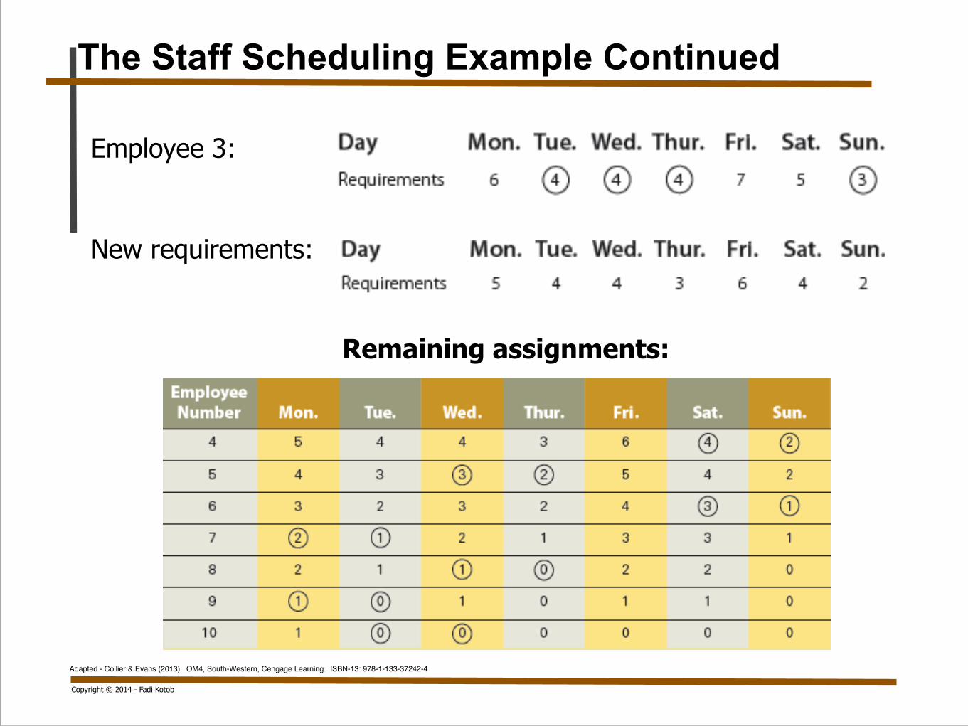
Remaining assignments:
The Staff Scheduling Example Continued
Employee 3:
New requirements:

Copyright © 2014 - Fadi Kotob
Adapted - Collier & Evans (2013). OM4, South-Western, Cengage Learning. ISBN-13: 978-1-133-37242-4
Exhibit 14.2 Final Accountant Schedule
The Staff Scheduling Example Continued

Copyright © 2014 - Fadi Kotob
Adapted - Collier & Evans (2013). OM4, South-Western, Cengage Learning. ISBN-13: 978-1-133-37242-4
!
Appointment Systems Appointments systems on the other hand can be viewed as a reservation for service time and capacity.
Appointment Systems
Four decisions:
1. Determine the appointment time interval.
2. Determine the length of each workday and time off-duty.
3. Decide how to handle overbooking.
4. Develop customer appointment rules that maximise customer satisfaction.

Copyright © 2014 - Fadi Kotob
Adapted - Collier & Evans (2013). OM4, South-Western, Cengage Learning. ISBN-13: 978-1-133-37242-4
After covering the scheduling applications and approaches, let’s start by explaining sequencing which is required when several activities must be processed using a common resource.
Sequencing
First, it is important to understand the sequencing performance criteria and the sequencing rules.

Copyright © 2014 - Fadi Kotob
Adapted - Collier & Evans (2013). OM4, South-Western, Cengage Learning. ISBN-13: 978-1-133-37242-4
!
The criteria is often classified into 3 categories:
1. Process-focused performance criteria
2. Customer-focused due date criteria
3. Cost-based criteria
Sequencing Performance Criteria

Copyright © 2014 - Fadi Kotob
Adapted - Collier & Evans (2013). OM4, South-Western, Cengage Learning. ISBN-13: 978-1-133-37242-4
Process-focused performance criteria looks at information about
the start and end times of jobs and focus on shop performance
such as equipment utilisation and work in process inventory.
Two common measures which are:
• Flow time • Makespan
Sequencing - The Process Focused Performance Criteria

Copyright © 2014 - Fadi Kotob
Adapted - Collier & Evans (2013). OM4, South-Western, Cengage Learning. ISBN-13: 978-1-133-37242-4
Flow time is the amount of time a job spent in the shop or
factory.
Fi = ∑pij + ∑wij = Ci - Ri
where Fi = flow time of job i ∑pij = sum of all processing times of job i at workstation or area j (run + setup times) ∑wij = sum of all waiting times of job i at workstation or area j Ci = completion time of job i Ri = ready time for job i where all materials, specifications, and so on are available
Sequencing - The Process Focused Performance Criteria

Copyright © 2014 - Fadi Kotob
Adapted - Collier & Evans (2013). OM4, South-Western, Cengage Learning. ISBN-13: 978-1-133-37242-4
!
Makespan is the time needed to process a given set of jobs.
M = C - S
Sequencing - The Process Focused Performance Criteria
where M = makespan of a group of jobs
C = completion time of last job in the group
S = start time of first job in the group

Copyright © 2014 - Fadi Kotob
Adapted - Collier & Evans (2013). OM4, South-Western, Cengage Learning. ISBN-13: 978-1-133-37242-4
Customer focused due dates considers the due dates promised
to customers or the internally pre-determined shipping dates.
Two common measures which are:
• Lateness
• Tardiness
Sequencing - The Customer Focused Due Date Criteria

Copyright © 2014 - Fadi Kotob
Adapted - Collier & Evans (2013). OM4, South-Western, Cengage Learning. ISBN-13: 978-1-133-37242-4
!
• Lateness is the difference between the completion time and the due date (either positive or negative).
• Tardiness is the amount of time by which the completion time exceeds the due date.
(Tardiness is defined as zero if job is completed before due date.)
Li = Ci - Di [14.3]
Ti = Max (0, Li) [14.4]
Sequencing - The Customer Focused Due Date Criteria
where
Li = lateness of job i
Ti = tardiness of job i
Ci = completion time of job i
Di = due date of job i

Copyright © 2014 - Fadi Kotob
Adapted - Collier & Evans (2013). OM4, South-Western, Cengage Learning. ISBN-13: 978-1-133-37242-4
Cost based criteria focuses on costs which typically include:
• Inventory
• Changeover or setup
• Processing
• Materials handling
Sequencing - The Cost Based Criteria

Copyright © 2014 - Fadi Kotob
Adapted - Collier & Evans (2013). OM4, South-Western, Cengage Learning. ISBN-13: 978-1-133-37242-4
!
The are many sequencing rules that can be used. These rules
are divided into 2 categories:
1. Rules for fixed set of jobs
2. Rules for intermittent set of jobs
Sequencing Rules
Copyright © 2014 - Fadi Kotob
Adapted - Collier & Evans (2013). OM4, South-Western, Cengage Learning. ISBN-13: 978-1-133-37242-4
!
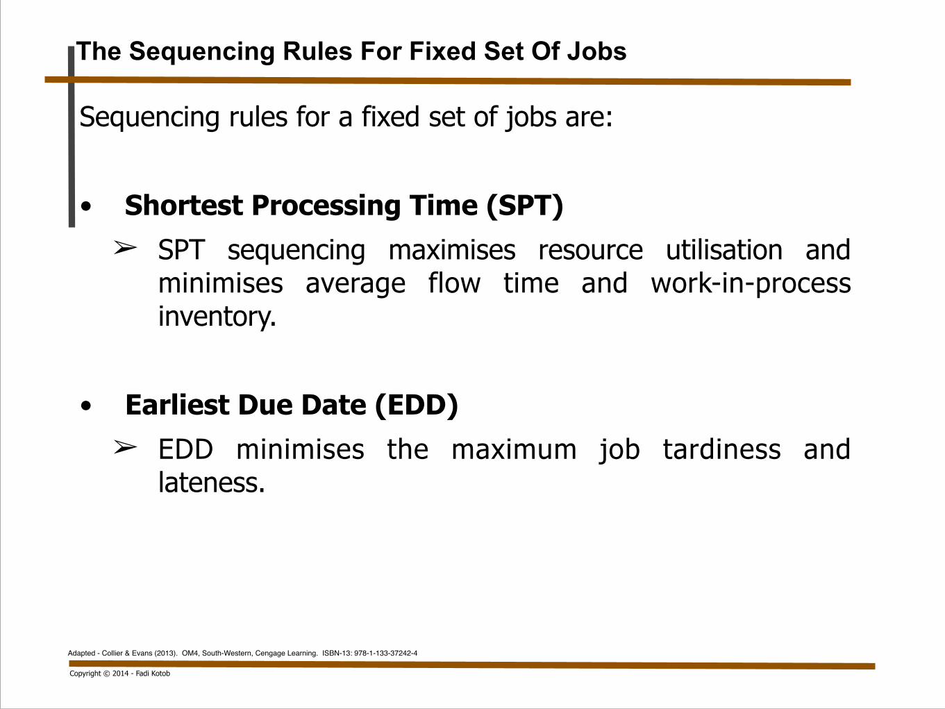
Sequencing rules for a fixed set of jobs are:
!
• Shortest Processing Time (SPT) ➢ SPT sequencing maximises resource utilisation and
minimises average flow time and work-in-process inventory.
!
• Earliest Due Date (EDD) ➢ EDD minimises the maximum job tardiness and
lateness.
The Sequencing Rules For Fixed Set Of Jobs

Copyright © 2014 - Fadi Kotob
Adapted - Collier & Evans (2013). OM4, South-Western, Cengage Learning. ISBN-13: 978-1-133-37242-4
!
Priority rules when new jobs arrive intermittently:
• First come-first served (FCFS) used in many service delivery systems and does not consider any job or customer criterion.
• Fewest number of operations remaining (FNO) but does not consider the length of time for each operation.
• Least work remaining (LWR) – the sum of all processing times for operations not yet performed.
• Least amount of work at the next process queue (LWNQ) – amount of work awaiting the next process in a job’s sequence. Rule tries to keep downstream work stations and associated resources busy.
The Sequencing Rules For Intermittent Set Of Jobs

Copyright © 2014 - Fadi Kotob
Adapted - Collier & Evans (2013). OM4, South-Western, Cengage Learning. ISBN-13: 978-1-133-37242-4
!
We will illustrate scheduling on a single resource scheduling
problem and on the two resourcing sequencing problem.
Application Of Sequencing Rules

Copyright © 2014 - Fadi Kotob
Adapted - Collier & Evans (2013). OM4, South-Western, Cengage Learning. ISBN-13: 978-1-133-37242-4
!
• Process a set of jobs on a single processor.
➢ FCFS (First come-first served) rule works well when
processing times are relatively equal.
➢ SPT (Shortest processing time) sequencing finds a
minimal average flow time sequence.
➢ EDD (Earliest due date) rule minimises the maximum
job tardiness and lateness.
Application Of Sequencing Rules Single-Resource Sequencing Problem

Copyright © 2014 - Fadi Kotob
Adapted - Collier & Evans (2013). OM4, South-Western, Cengage Learning. ISBN-13: 978-1-133-37242-4
Job Processing Time (days) Due Date 1 4 15 2 7 16 3 2 8 4 6 21 5 3 9
FCFS Sequencing Rule Example

Copyright © 2014 - Fadi Kotob
Adapted - Collier & Evans (2013). OM4, South-Western, Cengage Learning. ISBN-13: 978-1-133-37242-4
SPT Sequencing Rule Example
Job Processing Time (days) Due Date 1 4 15 2 7 16 3 2 8 4 6 21 5 3 9

Copyright © 2014 - Fadi Kotob
Adapted - Collier & Evans (2013). OM4, South-Western, Cengage Learning. ISBN-13: 978-1-133-37242-4
EDD Sequencing Rule Example
Job Processing Time (days) Due Date 1 4 15 2 7 16 3 2 8 4 6 21 5 3 9

Copyright © 2014 - Fadi Kotob
Adapted - Collier & Evans (2013). OM4, South-Western, Cengage Learning. ISBN-13: 978-1-133-37242-4
Exhibit 14.3 Comparison of Three Ways (By-the Numbers, SPT, and EDD) to Sequence the Five Jobs
Comparing The Three Sequencing Rules

Copyright © 2014 - Fadi Kotob
Adapted - Collier & Evans (2013). OM4, South-Western, Cengage Learning. ISBN-13: 978-1-133-37242-4
For a two-resource sequencing problem, S. M. Johnson developed a sequencing rule to minimise the time needed to process a given set of jobs (Makespan). The steps to achieve this are:
1. List the jobs and their processing times on Resources #1 and #2.
2. Find the job with the shortest processing time (on either resource).
3. If this time corresponds to Resource #1, sequence the job first; if it corresponds to Resource #2, sequence the job last.
4. Repeat steps 2 and 3, using the next-shortest processing time and working inward from both ends of the sequence until all jobs have been scheduled.
Application Of Sequencing Rules Two-Resource Sequencing Problem

Copyright © 2014 - Fadi Kotob
Adapted - Collier & Evans (2013). OM4, South-Western, Cengage Learning. ISBN-13: 978-1-133-37242-4
There are 5 jobs to be completed with each job requiring first a shearing operation (Resource #1) and then a punch-press operation (Resource #2).
STEP 1 1. List the jobs and their processing times on Resources #1
and #2.
Two-Resource Sequencing Example

Copyright © 2014 - Fadi Kotob
Adapted - Collier & Evans (2013). OM4, South-Western, Cengage Learning. ISBN-13: 978-1-133-37242-4
STEPS 2 & 3 2. Find the job with the shortest processing time (on either resource).
3. If this time corresponds to Resource #1, sequence the job first; if it corresponds to Resource #2, sequence the job last.
Two-Resource Sequencing Example Continued
Job 2 has the shortest processing time; since it is on Resource 2, schedule it last. Job 5 has the next shortest processing time; since it is on Resource 1, schedule it first:

Copyright © 2014 - Fadi Kotob
Adapted - Collier & Evans (2013). OM4, South-Western, Cengage Learning. ISBN-13: 978-1-133-37242-4
STEPS 4 4. Repeat steps 2 and 3, using the next-shortest processing time and working inward from both ends of the sequence until all jobs have been scheduled.
Continuing, choose job 3 and finally job 4:
Next, both job 1 on the shear have the next shortest time. Choose job 1:
Two-Resource Sequencing Example Continued

Copyright © 2014 - Fadi Kotob
Adapted - Collier & Evans (2013). OM4, South-Western, Cengage Learning. ISBN-13: 978-1-133-37242-4
If jobs are completed by order number, the punch press often experiences idle time awaiting the next job. The makespan is 37 days.
Exhibit 14.5 Gantt Job Sequence Chart for Hirsch Product Sequence 1-2-3-4-5
Two-Resource Sequencing Example Continued

Copyright © 2014 - Fadi Kotob
Adapted - Collier & Evans (2013). OM4, South-Western, Cengage Learning. ISBN-13: 978-1-133-37242-4
Johnson’s Rule results in a reduction in makespan from 37 days to 27 days, as shown in the Gantt chart.
Exhibit 14.6 Gantt Job Sequence Chart for Hirsch Product Sequence 5-1-4-3-2 Using Johnson’s Rule
Two-Resource Sequencing Example Continued

Copyright © 2014 - Fadi Kotob
Adapted - Collier & Evans (2013). OM4, South-Western, Cengage Learning. ISBN-13: 978-1-133-37242-4
!
• Finally, it is important to bear in mind that even with a great schedule, things could go wrong. This is why it is important to monitor how schedules are progressing on a continuing basis. Reschedules are a normal part of scheduling. !
• Gantt chart is a useful tool for monitoring schedules. This helps to track jobs that are behind, on, or ahead of schedule.
Schedule Monitoring & Control

Final Notes - Your Tasks For This Week
!– Review the lecture slides and the notes you have taken
!– Read chapters 13 and 17
!– Read the materials covered in the tutorial
!– Continue working on assignment 2, part 2
Copyright © 2014 - Fadi Kotob

Copyright © 2014 - Fadi Kotob
Thank You For Your Time