inverse design of dielectric materials by ... - · pdf fileinverse design of dielectric...

Progress In Electromagnetics Research, Vol. 127, 93–120, 2012

INVERSE DESIGN OF DIELECTRIC MATERIALS BYTOPOLOGY OPTIMIZATION

M. Otomori1, *, J. Andkjær2, O. Sigmund2, K. Izui1, andS. Nishiwaki1

1Kyoto University, Yoshida Honmachi, Sakyo-ku, Kyoto 606-8501,Japan2Technical University of Denmark, Nils Koppels Alle, Building 404,2800 Kgs. Lyngby, Denmark

Abstract—The capabilities and operation of electromagnetic devicescan be dramatically enhanced if artificial materials that provide certainprescribed properties can be designed and fabricated. This paperpresents a systematic methodology for the design of dielectric materialswith prescribed electric permittivity. A gradient-based topologyoptimization method is used to find the distribution of dielectricmaterial for the unit cell of a periodic microstructure composed of oneor two dielectric materials. The optimization problem is formulated asa problem to minimize the square of the difference between the effectivepermittivity and a prescribed value. The optimization algorithm usesthe adjoint variable method (AVM) for the sensitivity analysis andthe finite element method (FEM) for solving the equilibrium andadjoint equations, respectively. A Heaviside projection filter is usedto obtain clear optimized configurations. Several design problemsshow that clear optimized unit cell configurations that provide theprescribed electric permittivity can be obtained for all the presentedcases. These include the design of isotropic material, anisotropicmaterial, anisotropic material with a non-zero off-diagonal terms, andanisotropic material with loss. The results show that the optimizedvalues are in agreement with theoretical bounds, confirming that ourmethod yields appropriate and useful solutions.

Received 5 February 2012, Accepted 23 March 2012, Scheduled 10 April 2012* Corresponding author: Masaki Otomori ([email protected]).

94 Otomori et al.

1. INTRODUCTION

Artificial dielectric materials that are engineered to have an extremedielectric constant are of great interest for improving electromagneticdevices such as electrostatic actuators, waveguides, antennas, etc. Thispaper presents a systematic design methodology for the microstructuredesign of composites made from two dielectric materials with differentdielectric constants, or a single dielectric material and air. We usetopology optimization to find the shape and distribution of dielectricelements that exhibits a prescribed desirable dielectric constant.

Topology optimization is the most flexible type of structuraloptimization because it allows topological changes as well as shapechanges during the optimization process [1]. Topology optimizationmethods have been applied to a variety of problems such aselectromagnetic problems (e.g., [2–5]), fluid dynamics problem(e.g., [6]), phononics [7] and others. Topology optimization has alsobeen successfully applied to various microstructure design problemsaiming to develop materials that have extreme properties such asa negative thermal expansion coefficient [8], a negative Poisson’sratio [9], and materials with a prescribed value of a constitutivetensor such as Young’s modulus [10], magnetic permeability [11], adielectric constant [12], and so on. These problems are called inversehomogenization problems [10].

There are various methods for obtaining an effective permittivityvalue for dielectric composites. Analytic methods such as the Clausius-Mossotti, Maxwell-Garnett, and Bruggeman formulas, which arealso called mixing formulas, compute the effective permittivity ofcomposites based on the volume of the inclusions [13], however theaccuracy is valid only for certain inclusion shapes such as spheres,cylinders, and ellipsoids. A homogenization method such as a methodbased on asymptotic expansion [14, 15], and also an energy-basedmethod [16], can be used when dealing with more complicated shapeswhere the effective properties are obtained based on the results of finiteelement analysis. In this study, an energy-based method is used toobtain the effective permittivity of the dielectric materials.

There is considerable literature on the investigation of thetheoretical bounds for the effective properties of composites (e.g., [17]).The primal bounds for two-phase dielectric materials are given byarithmetic and harmonic means of each dielectric constant. Tighterbounds can be obtained based on certain available information aboutthe composites, such as their volume fractions and/or isotropy. In thispaper, we deal with two-dimensional design problems. To evaluate thepermittivity values obtained in optimization, we derive the theoretical

Progress In Electromagnetics Research, Vol. 127, 2012 95

bounds of the two-dimensional anisotropic effective property in theprincipal direction when that of the other principal direction is set toa prescribed value. Permittivity values obtained in optimizations arecompared with these derived theoretical bounds.

In a previous study on the microstructure design of dielectricmaterials [12], a genetic algorithm (GA) was used in the optimizationmethod. However, meta-heuristic approaches such as GAs, ParticleSwarm Optimization (PSO), and Simulated Annealing (SA) aregenerally not suitable for topology optimization since the number ofdesign variables is usually so large that the optimization becomestoo computationally costly [18]. Hence in [12] design resolution waslimited to extremely coarse discretizations. In this work, a gradient-based topology optimization method is used to find the distribution ofdielectric material for the unit cell of a periodic microstructure, wheredensities are updated based on the sensitivities. The computation ofsensitivities is significantly streamlined by using the adjoint variablemethod (AVM). In this way, we are able to solve problems with veryfine discretizations and hence obtain accurate results and detailedboundary descriptions. The objective of the optimization is to designdielectric materials that exhibit a prescribed effective permittivity.Therefore, the optimization problem is formulated as a problem tominimize the square of the difference between the effective permittivityand a prescribed value. The optimization algorithm uses the finiteelement method (FEM) for solving the equilibrium and adjointequations, respectively. A Heaviside projection filter [20] is usedto obtain clear optimized configurations. We study several designproblems including the design of an isotropic material, an anisotropicmaterial, an anisotropic material with non-zero off-diagonal terms, andan anisotropic material with loss.

The rest of this paper is as follows. Section 2 describes theformulation of the homogenization method for obtaining the effectivepermittivity, and the optimization problem for the design of dielectricmetamaterials. Section 3 discusses the theoretical bounds of theeffective properties for two-phase composites. Section 4 describes thenumerical implementation based on the formulation of the optimizationproblem, which uses the FEM and AVM to compute the sensitivity.Finally, several numerical examples are provided to confirm the validityand utility of the presented method.

96 Otomori et al.

2. FORMULATION

2.1. Effective Permittivity

In this study, the electrostatic effective permittivity is obtained on thebasis of the energy-based approach that employ conductivity averagetheorems [16] (see also [10]), where the effective permittivities areexpressed in terms of mutual energies as follows. This method assumethat the mutual energies accumulated in the original unit cell and inthe homogenized cell are equivalent. The mutual energy accumulatedin the original unit cell is given as

Qij =12

∫

Ωεr∇φi · ∇φjdΩ, (1)

where εr represents the element of electric permittivity tensor and φi

and φj are the electric potentials obtained when an electric voltageis applied in the xi and xj directions, respectively (Figure 1), whereij=11, 12, 21, 22, and φi denotes the conjugate complex number of φi.On the other hand, the mutual energy accumulated in the homogenizedcell is given as

QHij =

12εeff, ijV

0i V 0

j V, (2)

where V is the volume and V 0i is the applied voltage defined in a

boundary condition that produce homogeneous fields. By assumingQij = QH

ij , the elements of the effective permittivity tensor, εeff, ij inEq. (2), are determined as follows.

εeff =[

εeff, 11 εeff, 12

εeff, 21 εeff, 22

], (3)

where

εeff, 11 =1

V 01

2V

∫

Ωεr (x)∇φ1 (x) · ∇φ1 (x) dΩ (4)

εeff, 22 =1

V 02

2V

∫

Ωεr (x)∇φ2 (x) · ∇φ2 (x) dΩ (5)

εeff, 12 =1

V 01 V 0

2 V

∫

Ωεr (x)∇φ2 (x) · ∇φ1 (x) dΩ (6)

εeff, 21 =1

V 01 V 0

2 V

∫

Ωεr (x)∇φ1 (x) · ∇φ2 (x) dΩ, (7)

The electric potential φi are obtained by solving the followinggoverning equation using the FEM.

∇ · [εr (x)∇φi (x)] = 0, (8)


(a) (b)

L

L

Γ

Γ

Γ

Γ

Γ Γ

Γφ = φ 1 1_ Γ 2

φ = φ 1 1_ Γ1+V

0

1

φ = φ _ Γ1+V0

2 2 2

φ = φ _ Γ12 2

Γ

Figure 1. Analysis model and boundary conditions for the case ofan electric voltage applied in (a) the horizontal direction, and (b) thevertical direction.

The left and right boundaries, and the upper and lower boundariesare, respectively, set to a periodic boundary condition as follows, inthe case when an electric voltage is applied in the horizontal direction(Figure 1(a)).

φ1(x1, x2) = φ1(x1 − L1, x2) + V 01 on Γ3 (9)

φ1(x1, x2) = φ1(x1, x2 − L2) on Γ4, (10)

where V 01 is an applied voltage in the horizontal direction and, L1 and

L2 are the unit cell lengths in the x1 and x2 directions, respectively.The left and right boundaries, and the upper and lower boundaries

are, respectively, set to a periodic boundary condition as follows, inthe case when an electric voltage is applied in the vertical direction(Figure 1(b)).

φ2(x1, x2) = φ2(x1 − L1, x2) on Γ3 (11)φ2(x1, x2) = φ2(x1, x2 − L2) + V 0

2 on Γ4, (12)

where V 02 is an applied voltage in the vertical direction. The effective

permittivities are obtained by substituting obtained electric potentialsinto Eqs. (4)–(7).

2.2. Design Variables

In this work, the distribution of dielectric material inside the fixeddesign domain is expressed using relative element densities ρe ∈ [0, 1].That is, the relative electric permittivity εr inside the fixed designdomain is defined using ρe following the concept of the SIMP method.

εr = (ε1 − ε0) ρpe + ε0, (13)

98 Otomori et al.

where ε1 is the relative permittivity of the dielectric material, ε0is the relative permittivity of the background material, and p is apenalization parameter. For problems that have an active volumeconstraint, a large value of p > 1 penalizes intermediate elementdensities, since the volume is proportional to ρe but the permittivityvalues fall below the line of proportionality. The parameter p ≥ 3is typically used in structural optimization problems, since the bulkmodulus and shear modulus of interpolated stiffness tensor are requiredto satisfy the Hashin-Shtrikman bounds, which isotropic materialsshould satisfy [19]. Here, we use p = 3 in the following numericalexamples. It is because the profile of interpolated permittivity byp = 3 respect to the element density is similar to, even though it isnot the same as, that of the Hashin-Strikman bounds when the loss ofdielectric materials is small.

To ensure that the optimal design is independent of the mesh,and to obtain a clear optimal configuration, the Heaviside projectionfilter is used in this work [20]. Using this filter, the relative elementdensities ρe can be computed as shown in the following procedures.First, intermediate variables µe are computed using design variables ρe

that are typically located in nodes or the center of the finite elements,as follows.

µe =∑

j∈Ne

ρew/∑

j∈Ne

w, (14)

where N e is the neighborhood of elements specified by a circle with thegiven filter radius, and w is a weighting function that imposes higherweights for closer design variables. The relative element densities arethen obtained using the Heaviside function as follows.

ρe = Hs(µe) = 1− e−βµe + µee−β, (15)

where β is a parameter that adjusts the curvature of the Heavisidefunction. To ensure stable convergence of the optimization, themagnitude of parameter β is gradually increased from 1 to sufficientlylarge value (e.g., 500) during the optimization procedure. Publishedreferences provide more details concerning the use of densityfilters [20, 21].

2.3. Optimization Problem

Here, we discuss the formulation of the optimization problem that willbe applied to the dielectric material design problems. The purposeof the optimization is to obtain layouts of dielectric material thatachieve the desired dielectric permittivity. Thus, the objective of theoptimization problem can be formulated as to minimize the square of


the difference between the target permittivity and obtained effectivepermittivity. The optimization problem is described as follows.

infρe

F (ρe) = log∑

ij

∣∣ε∗eff, ij/ε∗tar, ij − 1∣∣2 (16)

subject to G =1

VD

∫

DρedΩ− Vmax ≤ 0 (17)

Poisson equation: Eq. (8) (18)Boundary conditions: Eqs.(9)–(12) (19)

where εeff and εtar respectively represent the effective permittivity andthe target permittivity. The ∗ denotes the use of either ′ or ′′ that applyto the real or imaginary part of the effective permittivity, respectively.The subscript ij = 11, 12, 21, 22 denotes the elements of the dielectrictensor. VD is the volume of the fixed design domain and Vmax isthe upper limit of volume fraction. Note that the logarithm of thesum of the differences is used as an objective functional to obtainbetter numerical scaling. When the differences become smaller duringoptimization, the magnitude of the sensitivities also diminish, whichslows convergence.

2.4. Sensitivity Analysis

The sensitivities of the objective functional for the gradient-basedtopology optimization are obtained using the adjoint variable method(AVM). The governing equation is discretized and solved using theFEM. The discretized governing equation can be described as follows.

Sφi = f , (20)where S is the stiffness matrix and f is the load vector. The sensitivityof the objective functional F is then given as

dF

dρ=

∂F

∂ρ+ 2Re

(λT

(∂S∂ρ

φi − ∂f∂ρ

)), (21)

where λ is an adjoint variable. The adjoint variable λ is obtained bysolving following adjoint problem.

ST λ = − ∂F

∂φi. (22)

With A as the integrand of the objective functional, the derivative ofthe objective functional with respect to the state variable ∂F

∂φican be

computed directly as follows.∂F

∂φi=

1V 2

∫

D

(∂A

∂φi+

∂A

∂∇φi· ∇

)dD, (23)

100 Otomori et al.

where,

∂A

∂φi= 0 (24)

∂A

∂∇φi= εr∇φi. (25)

In Eq. (21), ∂f∂ρ = 0 since the applied voltage is independent with

respect to the design variables. Computation of the derivative usingEq. (21) can be simplified by following Olesen’s implementationtechnique [22].

3. THEORETICAL BOUNDS

In this section, the theoretical bounds of the effective permittivity fortwo-phase dielectric composites are discussed.

210-1-2

1

2

Isotropic

Anisotropic

Anisotropic

Figure 2. Bounds of effective permittivity for two constituentmaterials with properties ε1 = −2 + 3i and ε2 = 1 + 1i. In theabsence of specific information concerning the dielectric materials, theeffective permittivity is confined to the region Ω. If the volume fractionof phase 1 is f1 = 0.6, the effective permittivity is confined to theregion Ω′. Furthermore, if the composite is a two-dimensional isotropicmaterial, the effective permittivity is confined to the region Ω′′.


3.1. Review of Theoretical Bounds of Effective Permittivityfor Two-phase Composite Material

3.1.1. Bounds of Complex Value Effective Permittivity

Let εeff be the effective permittivity of a two-phase composite withcomplex dielectric constants ε1 and ε2. The analytical bounds of εeffcan be illustrated as shown in Figure 2. Here, as an example, thedielectric constants for phases 1 and 2 are set to ε1 = −2 + 3i andε2 = 1 + 1i, respectively, and the volume fraction for phase 1 is set to0.6 for bounds Ω

′, Ω

′′, (the same example as Chap. 27 in [17]). These

bounds are obtained as follows. We note that for composites madefrom a single dielectric material and air, the bounds are obtained bysetting ε2 = 1.

In the absence of specific information concerning the topologicaldistribution of the constituent, the corresponding bounds are theWiener harmonic and arithmetic mean bounds expressed by followingequations.

εU0eff (v) =

(v

ε1+

1− v

ε2

)−1

(26)

εL0eff (w) = wε1 + (1− w)ε2, (27)

as parameters v and w are varied from 0 to 1.The boundary εU0

eff (v) represents the composite as a laminatematerial oriented so that the applied field V 0 is parallel to the directionof lamination (see Figure 3(a)). On the other hand, boundary εL0

eff (w)represents the composite as a laminate material oriented so that theapplied field V 0 is orthogonal to the direction of lamination (seeFigure 3(b)).

In addition, if the volume fraction of phase 1, f1, is known, theeffective permittivities at points A and B on the above boundaries εU0

eff

Figure 3. Laminate model.

102 Otomori et al.

and εL0eff in Figure 2 are determined as follows.

εAeff =

(f1

ε1+

f2

ε2

)−1

(28)

εBeff = f1ε1 + f2ε2, (29)

where f2 = 1−f1 is the volume fraction of phase 2. Tighter boundariesare expressed by an arc joining the point A and B that when extendedpasses through ε2 and an arc that passes through ε1, that can beexpressed by the following equations as the parameters v and w arevaried from 0 to 1.

εU1eff = ε2 +

f1ε2 (ε1 − ε2)ε2 + vf2 (ε1 − ε2)

(30)

εL1eff = ε1 +

f2ε1 (ε2 − ε1)ε1 + wf1 (ε2 − ε1)

. (31)

The boundary εU1eff (v) represents an elliptic assemblage with a core of

component 1 surrounded by component 2 (see Figure 4(a)). On theother hand, the boundary εL1

eff (w) represents an elliptic assemblage witha core of component 2 surrounded by component 1 (see Figure 4(b)).The major and minor diameters of the phase 1 structure, D1a, D1b,and of the phase 2 structure, D2a, D2b, have following relationshipsince the inner and outer ellipses are confocal [23].

D22a −D2

2b = D21a −D2

1b. (32)

Therefore, volume fraction f1 and parameter v are described as follows.

f1 =D1aD1b

D2aD2b(33)

v =D1aD2a

D1aD2a + D1bD2b. (34)

Moreover, if we know that the composite is a two-dimensionalisotropic material, then we can define the effective permittivities atpoints X and Y on the above boundaries, εU1

eff and εL1eff , respectively,

using the following equation.

εXeff = ε1 +

2f2ε1(ε2 − ε1)2ε1 + f1(ε2 − ε1)

(35)

εYeff = ε2 +

2f1ε2(ε1 − ε2)2ε2 + f2(ε1 − ε2)

. (36)

The tighter boundaries are expressed by an arc joining the pointX and Y that when extended passes through ε2 and an arc that passes


through ε1. These bounds are expressed by following equations as theparameters v and w are varied from 0 to 1.

εU2eff = εX

eff +1− v

1/(εYeff − εX

eff) + v/(εXeff − ε2)

(37)

εL2eff = εX

eff +1− w

1/(εYeff − εX

eff) + w/(εXeff − ε1)

. (38)

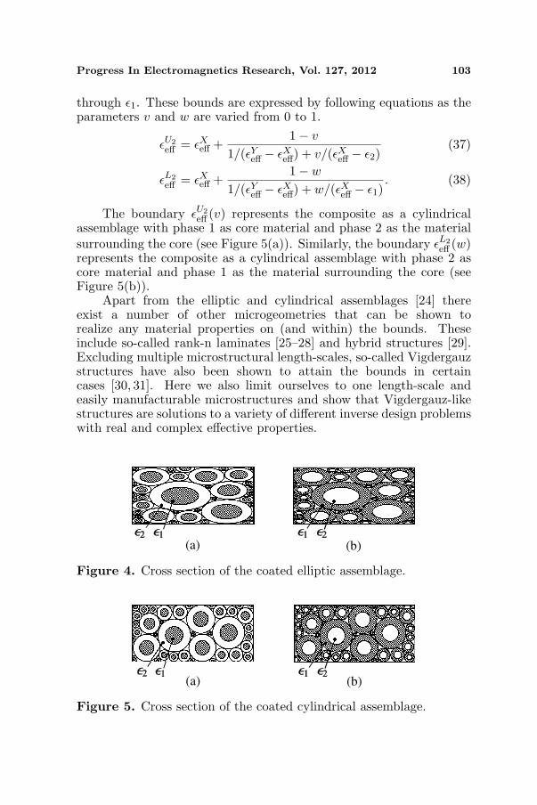
The boundary εU2eff (v) represents the composite as a cylindrical

assemblage with phase 1 as core material and phase 2 as the materialsurrounding the core (see Figure 5(a)). Similarly, the boundary εL2

eff (w)represents the composite as a cylindrical assemblage with phase 2 ascore material and phase 1 as the material surrounding the core (seeFigure 5(b)).

Apart from the elliptic and cylindrical assemblages [24] thereexist a number of other microgeometries that can be shown torealize any material properties on (and within) the bounds. Theseinclude so-called rank-n laminates [25–28] and hybrid structures [29].Excluding multiple microstructural length-scales, so-called Vigdergauzstructures have also been shown to attain the bounds in certaincases [30, 31]. Here we also limit ourselves to one length-scale andeasily manufacturable microstructures and show that Vigdergauz-likestructures are solutions to a variety of different inverse design problemswith real and complex effective properties.

(a) (b)

Figure 4. Cross section of the coated elliptic assemblage.

(a) (b)

Figure 5. Cross section of the coated cylindrical assemblage.

104 Otomori et al.

3.1.2. Bounds of Real Value Effective Permittivity

The bounds of real value effective permittivity versus the volumefraction f1 is obtained as follows. In the absence of specific information,εAeff(f1) in Eq. (28) is the lower bound and εB

eff(f1) in Eq. (29) is theupper bound of the effective permittivity of the composite materialsversus volume fraction f1. In addition, if we know the composite isisotropic material, the point εX

eff(f1) in Eq. (35) and εYeff(f1) in Eq. (36)

are the upper and lower bounds of the effective permittivity of thecomposite materials versus volume fraction f1.

3.2. Bounds of 2-D Anisotropic Real Value EffectivePermittivity in the Principal Direction When that of theOther Principal Direction Is Known

Based on the discussion in Subsection 3.1, the bounds of the anisotropiceffective permittivity in the principal direction when that of the otherprincipal direction is known are derived in this subsection for the casewhen the dielectric constants of the two materials both have real values.From Eq. (34),

1− v =D1bD2b

D1aD2a + D1bD2b(39)

Eq. (34) and Eq. (39) are symmetric with respect to the principaldirections, a and b, so ε(v) and ε(1−v) show the effective permittivitiesof the two principal directions. If we know the permittivity value ofone of the principal directions and let it be ε∗, the parameter v and win Eqs. (30) and (31) is obtained as,

v∗ =f1ε2(ε1 − ε2)− ε2(ε∗ − ε2)

f2(ε1 − ε2)(ε∗ − ε2)(40)

w∗ =f2ε1(ε2 − ε1)− ε1(ε∗ − ε1)

f1(ε2 − ε1)(ε∗ − ε1). (41)

We then derive the following bounds, substituting 1 − v∗ and 1 − w∗into Eqs. (30) and (31).

εLeff = ε2 +

2f1ε2 (ε1 − ε2)2ε2 + (1− v∗)f2 (ε1 − ε2)

(42)

εUeff = ε1 +

2f2ε1 (ε2 − ε1)2ε1 + (1− w∗)f1 (ε2 − ε1)

. (43)


4. NUMERICAL IMPLEMENTATION

The optimization flowchart is shown in Figure 6. First, the designvariables are initialized. Next, the filtered design variable ρe iscomputed using the projection function and the Heaviside function.Objective and constraint functionals are then computed using theFEM. If the objective functional has converged, the optimizationprocedure is terminated. If not, the sensitivities of the objectiveand constraint functionals are computed using the AVM. The designvariables are then updated using the method of moving asymptotes(MMA) [32] and the process returns to the second step.

5. NUMERICAL EXAMPLES

Numerical examples are now presented to demonstrate the validityand capability of our method for the design of microstructuresbased on dielectric materials. First, we compare the asymptoticexpansion-based and energy-based approaches used to obtain effectivepermittivity values for the dielectric composites considered here.The following design examples include the design of an isotropicmaterial, an anisotropic material, an anisotropic material with a non-zero off-diagonal terms, and an anisotropic material with loss. Theoptimization target in all examples is to minimize the square of thedifference between the effective permittivity and a target value. Thedesign domain is discretized using 200 × 200 square elements. Acircular rod shape with a volume fraction of 50% is used as the initialconfiguration unless otherwise specified in the following examples.

Compute objective function and constraint

function using FEM

Compute sensitivities using

Adjoint Variable Method

Update design variables using MMA

Convergence?

Compute via projection function and

Heaviside function

Initialize design variable

End

eρ

YES

NO

eρ~

eρ

Figure 6. Flowchart of optimization algorithm.

106 Otomori et al.

5.1. Comparison of Methods to Obtain EffectivePermittivity Values

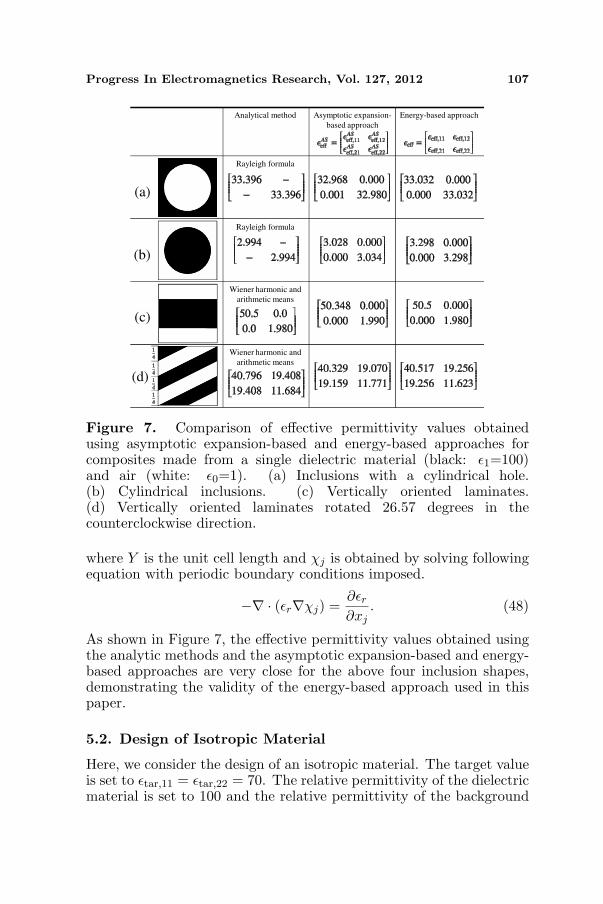
Here, we compare the asymptotic expansion-based approach andthe energy-based approach to show the validity of the energy-basedapproach used in this paper to obtain effective permittivity values forthe dielectric materials. Figure 7 shows a comparison of the effectivepermittivity values obtained using both approaches for compositesmade from a single dielectric material with ε1 = 100 and air, (ε0 = 1).Four inclusion shapes with volume fractions of 50% are consideredfor the comparison. That is, inclusions with a cylindrical hole(Figure 7(a)), cylindrical inclusions (Figure 7(b)), vertically orientedlaminates (Figure 7(c)), and vertically oriented laminates rotated 26.57degrees in the counterclockwise direction (Figure 7(d)) are considered.The effective permeability values obtained using analytic methods arealso compared for reference. For a square lattice with cylindrical holesand a lattice with cylindrical inclusions, the Rayleigh formula, definedas follows [33, 34], provides sufficient accuracy.

εeff = εe +2pεe

εi + εe

εi − εe− p− εi − εe

εi + εe(0.3058p4 + 0.0134p8)

, (44)

where εi is the permittivity of the cylindrical component, p is its volumefraction, and εe is the permittivity of the background material. Forlaminate inclusions, the effective permittivity can be obtained usingthe Wiener harmonic and arithmetic means (Eqs. (26) and (27)).

εeff =[50.5 0.00.0 1.980

]. (45)

The effective permittivity values for vertically oriented laminatesrotated 26.57 degrees in the counterclockwise direction are obtainedby rotating the effective permittivity tensor of the vertically orientedlaminates as follows.

εeff =[

cosθ sinθ−sinθ cosθ

]T[50.5 0.00.0 1.980

][cosθ sinθ−sinθ cosθ

]=

[40.796 19.40819.408 11.684

], (46)

where θ is set to 26.57 degrees. We note that analytic methods arevalid only for certain inclusion shapes.

For both the asymptotic expansion-based and energy-basedapproaches, the effective permittivity values are obtained using theFEM. Here, the analysis domain is discretized using 200 × 200 squareelements. The effective permittivity values using the asymptoticexpansion-based approach are obtained via following equation.

εASeff, ij =

1Y

∫

Ωεr(x)

(δij +

∂χj

∂xi

)dΩ, (47)


Analytical method Asymptotic expansion-

based approach

Energy-based approach

Rayleigh formula

Rayleigh formula

Wiener harmonic and

arithmetic means

Wiener harmonic and

arithmetic means

(a)

(b)

(c)

(d)

Figure 7. Comparison of effective permittivity values obtainedusing asymptotic expansion-based and energy-based approaches forcomposites made from a single dielectric material (black: ε1=100)and air (white: ε0=1). (a) Inclusions with a cylindrical hole.(b) Cylindrical inclusions. (c) Vertically oriented laminates.(d) Vertically oriented laminates rotated 26.57 degrees in thecounterclockwise direction.

where Y is the unit cell length and χj is obtained by solving followingequation with periodic boundary conditions imposed.

−∇ · (εr∇χj) =∂εr

∂xj. (48)

As shown in Figure 7, the effective permittivity values obtained usingthe analytic methods and the asymptotic expansion-based and energy-based approaches are very close for the above four inclusion shapes,demonstrating the validity of the energy-based approach used in thispaper.

5.2. Design of Isotropic Material

Here, we consider the design of an isotropic material. The target valueis set to εtar,11 = εtar,22 = 70. The relative permittivity of the dielectricmaterial is set to 100 and the relative permittivity of the background

108 Otomori et al.

material is set to 1. The maximum volume fraction is set to 82.5%, avalue chosen from theoretical bounds that will be discussed below.

The optimization results are shown in Figure 8. The obtainedeffective permittivity is

εeff =[

70.00 0.000.00 70.00

]. (49)

The permittivity values and optimal configuration show that theoptimization successfully obtained a clear structure that provides thetarget permittivity.

Figure 10 shows the theoretical bounds for the effectivepermittivity of composite materials composed of the above-mentioneddielectric and background materials, where the horizontal axis showsthe volume fraction of the dielectric material and the vertical axisshows the effective permittivity of the composite material. Thetheoretical bounds for anisotropic and isotropic materials are shownby solid and dashed lines, respectively. The effective permittivity ofthe optimized configuration is shown as the black square in Figure 10for comparison with the theoretical bound curve, and demonstratesthat the obtained result is in good agreement with theoretical bounds.

Figure 8. Optimized configuration of the isotropic material designproblem for volume fraction Vmax = 0.825 of ε1 = 100 (black), andε0 = 1 (white). The targets are εtar, 11 = εtar, 22 = 70 and the achievedproperties are εeff, 11 = εeff, 22 = 70.

Figure 9. Optimized configuration of the anisotropic material designproblem for volume fraction Vmax = 0.76 of ε1 = 100 (black), andε0 = 1 (white). The targets are εtar, 11 = 45 and εtar, 22 = 70 and theachieved properties are εeff, 11 = 45.00 and εeff, 22 = 70.00.


5.3. Design of Anisotropic Material

Next, the design of an anisotropic material is considered. The targetvalue is set to εtar,11 = 45, and εtar,22 = 70. The relative permittivityof the dielectric material is set to 100 and the relative permittivity ofthe background material is set to 1. The maximum volume fraction isset to 76%, a value chosen from theoretical bounds.


εeff =[

45.00 0.000.00 70.00

]. (50)

The permittivity values and optimal configuration show that theoptimization obtained the target permittivity for the anisotropicmaterial to a highly practical extent. Figure 10 shows the theoreticalbounds for the effective permittivity. The effective permittivity of theoptimized configuration is shown as the black dot in Figure 10 forcomparison with the theoretical bound curve. The highly sloped dot-

Volume fraction

1.00.90.80.70.60.50.40.30.20.10.00

50

100

Isotropic

Anisotropic

Anisotropic

Eff

ecti

ve

per

mit

tiv

ity

Figure 10. Theoretical bounds for isotropic and anisotropic materialdesign problems with properties ε1 = 100 and ε0 = 1. The solid anddashed lines show the theoretical bounds for isotropic and anisotropicmaterial, respectively. The dot-dashed line plots the upper and lowerlimit of the permittivity of the anisotropic material versus the volumefraction when ε22 = 70. The effective permittivity of the optimizedconfiguration, εeff, 11 = εeff, 22 = 70.00, of Subsection 5.2 is shownas the black square, and the effective permittivity of the optimizedconfiguration, εeff, 11 = 45.00 and εeff, 22 = 70.00, of Subsection 5.3is shown as the black dot, for comparison with the theoretical boundcurve.

110 Otomori et al.

dashed line plots the upper limit of the permittivity of the anisotropicmaterial versus the volume fraction when ε22 is 70. Similarly, thedot-dashed line that is partially obscured by solid line in the lowerright corner of the graph shows the lower limit of the permittivity ofthe anisotropic material versus the volume fraction when ε22 is 70.The black dot indicates the effective permittivity value of obtaineddielectric materials as optimization results and that the obtained resultis in good agreement with theoretical bounds.

5.4. Design of Anisotropic Material with Non-zeroOff-diagonal Terms

Here, the design of an anisotropic material with non-zero off-diagonalterms is considered. The target dielectric permittivity is set to

εtar =[

εa + δcos2φ δsin2φδsin2φ εa − δcos2φ

], (51)

where φ is set to 15 degrees and εa and δ are respectively set to 125and 40. That is,

εtar =[

159.64 −20−20 90.36

]. (52)

The relative permittivity of the dielectric material is set to 240 andthe relative permittivity of the background material is set to 20. Themaximum volume fraction is set to 69%, a value chosen from theoreticalbounds.


εeff =[

159.63 −20−20 90.36

]. (53)

Figure 11. The optimized configuration of the anisotropic materialdesign problem with non-zero off-diagonal terms for volume fractionVmax = 0.69 of ε1 = 240 (black), and ε0 = 20 (white). The targetsare εtar, 11 = 159.64, εtar, 22 = 90.36 and εtar, 12 = εtar, 21 = −20.00and the achieved properties are εeff, 11 = 159.63, εeff, 22 = 90.36 andεeff, 12 = εeff, 21 = −20.00.


Volume fraction

1.00.90.80.70.60.50.40.30.20.10.0

20

80

240

Isotropic

Anisotropic

Anisotropic

140

200

165

Eff

ecti

ve

per

mit

tiv

ity

eff

Figure 12. Theoretical bounds for anisotropic material designs withproperties ε1 = 240 and ε0 = 20. The solid and dashed lines show thetheoretical bounds for isotropic and anisotropic material, respectively.The dot-dashed line plots the upper limit of the permittivity of theanisotropic material versus the volume fraction when ε22 = 85. Theeffective permittivity of the optimized configuration, εeff, 11 = 164.99and εeff, 22 = 85.00, in the principal direction is shown as the black dotfor comparison with the theoretical bound curve.

The results show the optimization successfully obtained an optimizedconfiguration that provides the desired permittivity for an anisotropicmaterial that has non-zero off-diagonal terms.

Figure 12 shows the theoretical bounds for the effectivepermittivity. Here, the obtained effective permittivities in the principaldirection are considered, namely,

εeff =[

164.99 0.000.00 85.00

]. (54)

The effective permittivity of the optimized configuration is shownas the black dot for comparison with the theoretical bound curve. Thedot-dashed lines plot the upper and lower limit of the permittivity ofthe anisotropic material versus the volume fraction when ε22 is 85.

5.5. Design of Material with Loss Targeting Extreme Values

Finally, this design example considers materials with loss. To considerthe design of a lossy material, we first consider design problems wheretarget values are known from a theoretical point of view. In theseexamples, the relative permittivity of the dielectric material is set

112 Otomori et al.

i5.05.1 +

i2.04.1 +

i0.3081.462+

i0.3791.448+

Target1

Target2

Target 3

Anisotropic + Volume 50%

Anisotropic

Isotropic + Volume 50%

0.0

1.0

0.5

1.0 2.01.5

Figure 13. Theoretical bounds for lossy materials with propertiesε1 = 2 + 1i and ε0 = 1. The solid line shows the theoretical boundsfor two constituent materials, and the dashed-dot line and dashed lineshow the theoretical bounds for anisotropic and isotropic material witha volume fraction of 50%, respectively. The black dots indicate thetarget values used in the optimization in Subsection 5.5.

to 2 + 1i and the relative permittivity of the background materialis set to 1. The maximum volume fraction is set to 50%. Figure 13shows the upper and lower bounds for the effective permittivity ofcomposite materials composed of dielectric and background materials.The theoretical bounds for an anisotropic material, an anisotropicmaterial with a volume fraction of 50%, and an isotropic material witha volume fraction of 50% are respectively shown by the solid line, thedot-dashed line, and the dashed line.

Based on these theoretical bounds, three target values were usedto validate the present method. As shown in Figure 13, the targetvalues for the three examples were as follows:

For Example 1, the anisotropic material design problem, εtar,11 =1.5 + 0.5i. For Example 2, the isotropic material design problemwith maximum loss, εtar,11 = εtar,22 = 1.4483 + 0.3793i. And, forExample 3, the isotropic material design problem with minimum loss,εtar,11 = εtar,22 = 1.4615 + 0.3077i.

Figures 14, 15 and 16 show the respective optimization results foreach example. The obtained effective permittivity in Example 1 is

εeff =[

1.500 + 0.500i 0.00.0 1.400 + 0.200i

]. (55)


Figure 14. The optimized configuration of a lossy material designproblem: target1, for volume fraction Vmax = 0.5 of ε1 = 2 + 1i(black — lossy material) and ε0 = 1 (white). The target is εtar, 11 =1.5 + 0.5i and the obtained properties are εeff, 11 = 1.500 + 0.500i,εeff, 22 = 1.400 + 0.200i, and εeff, 12 = εeff, 21 = 0.0.

Figure 15. The optimized configuration of a maximum loss materialdesign problem: target2, for volume fraction Vmax = 0.5 of ε1 =2 + 1i (black — lossy material) and ε0 = 1 (white). The targetis εtar, 11 = εtar, 22 = 1.448 + 0.379i and the obtained properties areεeff, 11 = εeff, 22 = 1.446 + 0.377i and εeff, 12 = εeff, 21 = 0.0.

Figure 16. The optimized configuration of a minimum loss materialdesign problem: target3, for volume fraction Vmax = 0.5 of ε1 =2 + 1i (black — lossy material) and ε0 = 1 (white). The targetis εtar, 11 = εtar, 22 = 1.462 + 0.308i and the obtained properties areεeff, 11 = εeff, 22 = 1.459 + 0.308i and εeff, 12 = εeff, 21 = 0.0.

Although only ε11 was considered as the target value in theoptimization, the obtained value of ε22 is in good agreement with thetheoretical value of ε22, that is, ε22 = 1.4 + 0.2i.

The obtained effective permittivity for Example 2 is

εeff =[

1.446 + 0.377i 0.00.0 1.446 + 0.377i

], (56)

114 Otomori et al.

and the obtained effective permittivity for Example 3 is

εeff =[

1.459 + 0.308i 0.00.0 1.459 + 0.308i

]. (57)

These results show that the optimization can successfully find anoptimized configuration that has a desired permittivity even for thedesign of a lossy material.

Observing the optimized structures for maximum damping(Example 2) and minimum damping (Example 3) we note that theresults match intuition. For the lossy design, the lossy constituentprovides the matrix and the non-lossy is an isolated inclusion — andvise versa.

5.6. Design of Anisotropic Material with Loss: Effect ofInitial Configurations

Here, the design of anisotropic materials with loss is considered. Therelative permittivity of the dielectric materials is set to 140−0.196i andthe relative permittivity of the background material is set to 20−0.012i.Three different initial configurations are used in this design problem.The target values are set to εtar,11 = 60−0.06i and εtar,22 = 70−0.08i.

Figures 17, 18 and 19 show the optimization results basedon different initial configurations. Figure 17(a) shows the rod-shaped initial configuration and Figure 17(b) shows its optimizedconfiguration. The volume fraction of the optimized configuration is60.13%. The obtained effective permittivity is

εeff =[

59.80− 0.060i 0.00.0 69.64− 0.080i

]. (58)

(a) (b)

Figure 17. (a) The rod-shaped initial configuration, and (b)the optimized configuration of an anisotropic lossy material designproblem, for ε1 = 140−0.196i (black) and ε0 = 20−0.012i (white). Thetarget is εtar,11 = 60.00 − 0.060i and εtar,22 = 70.00 − 0.080i, and theobtained properties are εeff, 11 = 59.80− 0.060i, εeff, 22 = 69.64− 0.080iand εeff, 12 = εeff, 21 = 0.0.


(a) (b)

Figure 18. (a) The cross-shaped initial configuration, and (b) theoptimized configuration of an anisotropic lossy material design problemfor ε1 = 140− 0.196i (black) and ε0 = 20− 0.012i (white). The targetis εtar,11 = 60.00−0.060i and εtar,22 = 70.00−0.080i, and the obtainedproperties are εeff, 11 = 59.97 − 0.060i, εeff, 22 = 70.00 − 0.080i andεeff, 12 = εeff, 21 = 0.0.

(a) (b)

Figure 19. (a) The initial configuration in which the densitygradually changes over the design domain, and (b) the optimizedconfiguration of an anisotropic lossy material design problem, forε1 = 140 − 0.196i (black) and ε0 = 20 − 0.012i (white). The target isεeff, 11 = 60.00 − 0.060i and εeff, 22 = 70.00 − 0.080i, and the obtainedproperties are εeff, 11 = 60.00 − 0.060i, εeff, 22 = 69.82 − 0.080i andεeff, 12 = εeff, 21 = 0.0.

Figure 18(a) shows the cross-shaped initial configuration andFigure 18(b) shows its optimized configuration. The volume fractionof the optimized configuration is 61.50%. The obtained effectivepermittivity is

εeff =[

59.97− 0.060i 0.00.0 70.00− 0.080i

]. (59)

Figure 19(a) shows the initial configuration in which the densitygradually changes over the design domain, from a maximum valueat the center (ρ = 1) to zero density at the boundaries (ρ = 0).Figure 19(b) show the optimized configuration based on this initialconfiguration. The volume fraction of the optimized configuration is

116 Otomori et al.

Anisotropic + Volume 61.5%

Anisotropic

0.0

-0.05

0 50

-0.10

-0.15

-0.20

100 150

Figure 20. Theoretical bounds of anisotropic lossy material withproperties ε1 = 140 − 0.196i and ε0 = 20 − 0.012i. The solidline shows the theoretical bounds for two constituent materials, andthe dashed-dot line shows the theoretical bounds for an anisotropicmaterial with a volume fraction of 61.5%. Two black dots show theeffective permittivity of the optimized configuration when using thecross-shaped initial configuration.

61.56%. The obtained effective permittivity is

εeff =[

60.00− 0.060i 0.00.0 69.82− 0.080i

]. (60)

The different optimized structures obtained from the three differentinitial configurations indicate that this problem has several localoptima. Although the obtained optimal values differ slightly from thetarget value, clear optimized configurations that achieve the prescribedpermittivity value are obtained.

Figure 20 shows the upper and lower bounds of the effectivepermittivity of composite materials composed of the two differentlossy dielectric materials. The solid line shows the theoretical boundsfor two constituent materials, and the dashed-dot line shows thetheoretical bounds for the anisotropic material with loss that has avolume fraction of 61.5%. The two black dots represent the effectivepermittivity values of the optimized configuration based on the cross-shaped initial configuration. Here, we evaluate only the effectivepermittivity values obtained in the optimization using the cross-shapedinitial configuration, but the evaluations are very similar to those forthe other two cases.


6. CONCLUSION

In this paper, we presented a gradient-based topology optimizationmethod that can be applied to the design of microstructures basedon a periodic array of dielectric materials to achieve desired electricpermittivities. A simple homogenization method was used to obtainthe effective permittivity and the validity of the proposed method wasdemonstrated through several design problems, namely, those dealingwith an isotropic material, an anisotropic material, an anisotropicmaterial with a non-zero off-diagonal term, and an anisotropic materialwith loss. Clear optimized configurations with prescribed electricpermittivities were obtained for all the presented cases. Moreover,we derived the theoretical bounds of the two-dimensional anisotropiceffective property in the principal direction when the effective propertyin the other principal direction was set to a prescribed value, toevaluate the effective permittivity values obtained by the optimization.Our results showed that the optimized values are in good agreementwith theoretical bounds, confirming that our method yields appropriateand useful solutions.

The Vigdergauz-like optimized structures obtained in this paperprovide a directly manufacturable alternative to the multi-lengthscale microstructures from the literature. The scheme should bedirectly extendable to three-dimensions, more than two constituentsand metamaterial design.

ACKNOWLEDGMENT

This work was partially supported by JSPS, Grant-in-Aid for ScientificResearch (B), 22360041, and the “Institutional Program for YoungResearcher Overseas Visits.” The first author is partially supported byAISIN AW CO., LTD. The third author is partially supported by theVillum Foundation. We sincerely appreciate this assistance.

REFERENCES

1. Bendsøe, M. P. and N. Kikuchi, “Generating optimal topologiesin structural design using a homogenization method,” Comput.Methods Appl. Mech. Engrg., Vol. 71, No. 2, 197–224, 1988.

2. Yoo, J., N. Kikuchi, and J. L. Volakis, “Structural optimizationin magnetic devices by the homogenization design method,” IEEET. Magn., Vol. 36, No. 3, 574–580, 2000.

3. Nomura, T., S. Nishiwaki, K. Sato, and K. Hirayama, “Topologyoptimization for the design of periodic microstructures composed

118 Otomori et al.

of electromagnetic materials,” Finite Elem. Anal. Des., Vol. 45,No. 3, 210–226, 2009.

4. Nishiwaki, S., T. Nomura, S. Kinoshita, K. Izui, M. Yoshimura,K. Sato, and K. Hirayama, “Topology optimization for cross-section designs of electromagnetic waveguides targeting guidingcharacteristics,” Finite Elem. Anal. Des., Vol. 45, No. 12, 944–957, 2009.

5. Yamasaki, S., T. Nomura, A. Kawamoto, K. Sato, andS. Nishiwaki, “A level set-based topology optimization methodtargeting metallic waveguide design problems,” Int. J. Numer.Meth. Eng., Vol. 87, No. 9, 844–868, 2011.

6. Borrvall, T. and J. Petersson, “Topology optimization of fluids instoles flow,” Int. J. Numer. Meth. Eng., Vol. 41, No. 1, 77–107,2003.

7. Sigmund, O. and J. S. Jensen, “Systematic design of phononicband-gap materials and structures by topology optimization,”Phil. Trans. R. Soc. Lond. A, Vol. 361, 1001–1019, 2003.

8. Sigmund, O. and S. Torquato, “Design of materials with extremethermal expansion using a three-phase topology optimizationmethod,” J. Mech. Phys. Solids., Vol. 45, No. 6, 1037–1067, 1997.

9. Larsen, U. D., O. Sigmund, and S. Bouwstra, “Design andfabrication of compliant micromechanisms and structures withnegative Poisson’s ratio,” J. Microelectromech. S., Vol. 6, No. 2,99–106, 1997.

10. Sigmund, O., “Materials with prescribed constitutive parameters:an inverse homogenization problem,” INT. J. Solids Struct.,Vol. 31, No. 17, 2313–2329, 1994.

11. Choi, J. S. and J. Yoo, “Design and application of layeredcomposites with the prescribed magnetic permeability,” Int. J.Numer. Meth. Eng., Vol. 82, No. 1, 1–25, 2010.

12. El-Kahlout, Y. and G. Kiziltas, “Inverse synthesis of electromag-netic materials using homogenization based topology optimiza-tion,” Progress In Electromagnetics Research, Vol. 115, 343–380,2011.

13. Sihvola, A., Electromagnetic Mixing Formulas and Applicataions,The Institution of Engineering and Technology, London, 1999.

14. Bensoussan, A., J. L. Lions, and G. Papanicolau, AsymptoticAnalysis for Periodic Structures, North-Holland PublishingCompany, Amsterdam, 1978.

15. Sanchez-Palencia, E., “Non-homogeneous media and vibrationtheory,” Lecture Notes in Physics, Vol. 127, Springer-Verlag,


Berlin, 1980.16. Hashin, Z., “Analysis of composite materials — A survey,” J.

Appl. Mech., Vol. 50, No. 3, 481–505, 1983.17. Milton, G. W., The Theory of Composites, Cambridge University

Press, Cambridge, 2001.18. Sigmund, O., “On the usefulness of non-gradient approaches in

topology optimization,” Struct. Multidisc. Optim., Vol. 43, No. 5,589–596, 2011.

19. Bendsøe, M. P. and O. Sigmund, “Material interpolation schemesin topology optimization,” Arch. Appl. Mech., Vol. 69, No. 9–10,635–654, 1999.

20. Guest, J. K., J. H. Prevost, and T. Belytschko, “Achievingminimum length scale in topology optimization using nodal designvariables and projection functions,” Int. J. Numer. Meth. Eng.,Vol. 61, No. 2, 238–254, 2004.

21. Sigmund, O., “Morphology-based black and white filters fortopology optimization,” Struct. Multidisc. Optim., Vol. 33, No. 4–5, 401–424, 2007.

22. Olesen, L. H., “A high-level programming-language implemen-tation of topology optimization applied to steady-state Navier-Stokes flow,” Int. J. Numer. Meth. Eng., Vol. 65, No. 7, 975–1001,2006.

23. Milton, G. W., “Bounds on the complex permittivity of a two-component composite material,” J. Appl. Phys., Vol. 52, No. 8,5286–5293, 1981.

24. Hashin, Z., “The elastic moduli of heterogeneous materials,” J.Appl. Mech., Vol. 29, No. 1, 143–150, 1962.

25. Francfort, G. and F. Murat, “Homogenization and optimal boundsin linear elasticity,” Archive for Rational Mechanics and Analysis,Vol. 94, No. 4, 307–334, 1986.

26. Lurie, K. A. and A. V. Cherkaev, “Optimization of properties ofmulticomponent isotropic composites,” J. Optimiz. Theory App.,Vol. 46, No. 4, 571–580, 1985.

27. Milton, G. W., Modelling the Properties of Composites byLaminates, Vol. 1 of IMA, 150–174, Springer-Verlag, New York,1985.

28. Norris, A. N., “A differential scheme for the effective moduli ofcomposites,” Mech. Mater., Vol. 4, No. 1, 1–16, 1985.

29. Sigmund, O., “A new class of extremal composites,” J. Mech.Phys. Solids, Vol. 48, No. 2, 397–428, 2000.

120 Otomori et al.

30. Grabovsky, Y. and R. V. Kohn, “Microstructures minimizing theenergy of a two phase elastic composite in two space dimensions.II: the Vigdergauz microstructure,” J. Mech. Phys. Solids, Vol. 43,No. 6, 949–972, 1995.

31. Vigdergauz, S., “Energy-minimizing inclusions in a planar elasticstructure with macroisotropy,” Struct. Optimization, Vol. 17,No. 2–3, 104–112, 1999.

32. Svanberg, K., “A class of globally convergent optimizationmethods based on conservative convex separable approximations,”SIAM J Optimiz., Vol. 12, No. 2, 555–573, 2002.

33. Rayleigh, L., “On the influence of obstacles arranged inrectangular order upon the properties of a medium,” Philos. Mag.,Vol. 34, No. 211, 481–502, 1892.

34. Wallen, H., H. Kettunen, and A. Sihvola, “Composite near-field superlens design using mixing formulas and simulations,”Metamaterials, Vol. 3, No. 3–4, 129–139, 2009.

inverse design of dielectric materials by ... - · pdf fileinverse design of dielectric...

Documents