inverse estimation of boundary heat flux for heat ...model for heat flux is used. the inverse...

JKAU: Eng. Sci., Vol. 21 No.1 pp: 73-95 (1431A.H./2010 A.D.)

DOI: 10.4197 / Eng. 21-1.5

73

Inverse Estimation of Boundary Heat Flux for Heat

Conduction Model

A. S. A. Alghamdi

Faculty of Engineering, Umm Al-Qura University, Makkah, Saudi Arabia

[email protected]

Abstract. Mathematical model of direct and inverse problems is

developed for the flat plate probe which is subjected to time-

dependent heat flux at one end, while the other end is kept insulated.

The direct solution, which is concerned with determination of the

temperature distribution in the probe, is developed using an approach

based on the method of variation of parameters. The direct solution is

used to solve the inverse heat conduction problem (IHCP) for any

assumed heat flux. In this paper, the piecewise linear interpolation

model for heat flux is used. The inverse algorithm is developed using

the Levenberg-Marquardt method. Different test cases for known heat

flux profile are used to validate the inverse algorithm. A satisfactory

agreement between exact and estimated heat flux profiles is achieved.

The algorithm is used to estimate the heat flux for a flat plate probe

developed at Ohio University.

Keywords: Direct problem, Inverse problem, Variation of parameters,

IHCP

1. Introduction

An inverse problem in heat conduction consists of solving a direct

problem and then finding some way to determine the inverse solution [1]

.

In inverse heat conduction problem [1]

, the direct problem is used to

determine the temperature distribution inside the solid body when certain

initial and boundary conditions are given, such as temperature or heat

flux, which are known as a function of time. In practice, the temperature

in the solid can be monitored by sensors; however the surface heat flux

cannot be determined experimentally. Theoretically, the surface heat flux

A. S. A. Alghamdi 74

history can be calculated from a set of temperature values. This type of

problem is called “inverse heat conduction problem (IHCP)”. The

solution of the inverse heat conduction problem is difficult due to its

sensitivity to measurements [2,3]

.

Several numerical methods have been developed to solve the

inverse problem due to its sensitivity to measurements. These methods

are discussed in detail by M N Ozisiks et al. [1]

and J. Taler et al. [4]

.

Tervola [5]

developed a numerical method to determine thermal

conductivity from measured temperature profiles. The boundary element

method (BEM) was used by Lesnic et al. [6]

to determine the boundary

conditions in a transient conduction problem where energies are specified

in two areas of a one-dimensional slab. Tseng et al. [7]

, Hunag et al. [8]

,

and Keanini [9]

described applications of IHCP to the manufacturing

processes.

Estimation of heat flux from measured transient temperature

history has received great interest during last three decades [1,4]

. S.

Abboudi et al. [10]

developed one dimensional heat conduction model to

analyze numerically and experimentally transient heating of a flat

specimen. The heat flux absorbed by the specimen was estimated using

inverse analysis. Stolz [11]

developed a numerical solution for the inverse

problem of heat conduction for some simple shapes. Alam et al. [12]

,

Kumar [13]

, and Zhong [14]

developed an inverse solution to determine the

surface heat flux for quench probes in quenching experiment. These

authors used a the polynomial model (representing heat flux with sixth

degree polynomial) to solve the inverse problem for the probe [12,13]

.

They suggested that the results can be improved by representing the heat

flux )(tq by piecewise continuous polynomial of different degrees. The

next step is to replace the polynomial model by cubic spline model [14]

.

The solution obtained by the procedure described is complicated and

posed difficulties in the representation of heat flux in cubic spline. Also,

the cubic spline exhibited sensitivity and stability problems. Therefore, a

piecewise continuous straight line representation of )(tq was suggested

in order to improve the stability of the solution.

A classic problem in IHCP is the determination of surface heat flux

in a one-dimensional slab. Quenching experiments are often carried out

to determine the surface heat fluxes from experimental measurements of

the temperature history. This is a typical inverse problem and therefore it

Inverse Estimation of Boundary Heat Flux for Heat Conduction Model 75

is required to develop an algorithm with special considerations. This

paper is concerned with several objectives. Firstly, inverse heat

conduction model is developed based on the formulation of direct and

inverse problem. Secondly the inverse algorithm is constructed and

tested. Finally, numerical estimation of boundary heat flux for the flat

plate probe is investigated based on experimental measurements of the

temperature history obtained from Quenching experiment [15]

.

2. Mathematical Model

2.1 Direct Problem

Consider a one-dimensional heat conduction problem through a

uniform plate, as shown in Fig. 1. At one end, 0=x , the surface is

insulated, and the second end, Lx = , is subjected to heat flux ),( tLq .

This problem is described by the following set of equations:

2

2 ),(),(

x

txT

t

txT

∂

∂=

∂

∂α , in Lx <<0 , for 0>t (1a)

0),0(=

∂

∂

x

tT, at 0=x , for 0>t (1b)

)(),(

tqx

tLTk =

∂

∂, at Lx = , for 0>t (1c)

)()0,(0xTxT = , for 0=t , Lx <<0 (1d)

where

=α thermal diffusivity =T temperature

x = space coordinate k = thermal conductivity

= L thickness of plate =q heat flux

Fig. 1. One-dimensional flat plate probe with boundary conditions.

Lx L x == 0

q(t) x

txTk =

∂

∂ ),(0

),(=

∂

∂

x

txT


For the case where the boundary condition at Lx = , i.e., )(tq , the

initial condition )(0xT , and the thermo-physical properties α , and k are

all specified, the problem given by Equation (1) is concerned with the

determination of the temperature distribution ),( txT in the interior

region of the solid as a function of time and position.

2.2 Inverse Problem

The inverse problem is concerned with the determination of the

unknown function )(tq at the surface Lx = . To determine the heat flux

)(tq , measured temperatures iimeas

TtxT

∗

≡),( are given at an interior

point measx at different times ),,2,1( Iit

i…= , over a specified time

interval ftt ≤<0 . The mathematical formulation of the inverse problem

is given below:

2

2 ),(),(

x

txT

t

txT

∂

∂=

∂

∂α , in Lx <<0 , for

ftt ≤<0 (2a)

0),0(=

∂

∂

x

tT, at 0=x , for

ftt ≤<0 (2b)

)()(),(

unknowntqx

tLTk ==

∂

∂, at Lx = , for

ftt ≤<0 (2c)

)()0,(0xTxT = , for 0=t , Lx <<0 (2d)

and temperature measurements at an interior location measx at different

times it are given by

∗

≡iimeas

TtxT ),( at measxx = for ),,2,1( Iitt

i…== (3)

In our problem, the boundary surface function heat flux )(tq is

unknown. Therefore, this version of the problem is referred to as a

boundary inverse heat conduction problem. The main objective of the

direct problem is to construct the temperature field ( ),( txT , the effect) in

the plate, when all parameters (causes) are specified (0

,,, Tqkα ). On the

other hand, the objective of the inverse problem is to estimate heat flux

(the cause) from the knowledge of the measured temperature (the effect)

at some specified section of the medium ( 0xmeas

= ).

Alam et al. [12]

and Kumar [13]

developed an analytical solution,

which consists of finding the temperature in a one-dimensional plate for a


given heat flux which is assumed to be a polynomial function of time. It

was suggested that the results can be improved by representing the )(tq

by piecewise continuous polynomial of different degrees. Zhong [14]

conducted the study with a cubic spline function assigned to represent the

heat flux. However, the heat flux and the heat transfer coefficients

obtained from these approaches were not satisfactory.

3. Solution of the Direct problem

The method of variation of parameters, which is suitable for both

steady-state and non-steady-state problems, is used to solve the direct

heat conduction problem [16]

. The problem will be decomposed to two

parts: a problem formulation with prescribed initial condition and zero

boundary conditions, and a second problem formulation with prescribed

boundary conditions and zero initial condition. Since the problem is

linear one can write:

),(),(),( txvtxutxT += (4)

where ),( txu is the solution of

2

2 ),(),(

x

txu

t

txu

∂

∂=

∂

∂α , in Lx <<0 , for 0>t (5a)

0),0(=

∂

∂

x

tu, at 0=x , for 0>t (5b)

0),(=

∂

∂

x

tLu, at Lx = , for 0>t (5c)

)()0,(0xTxT = , for 0=t , Lx <<0 (5d)

while ),( txv is the solution of

2

2 ),(),(

x

txv

t

txv

∂

∂=

∂

∂α , in Lx <<0 , for 0>t (6a)

0),0(=

∂

∂

x

tv, at 0=x , for 0>t (6b)

)(),(

tqx

tLvk =

∂

∂, at Lx = , for 0>t (6c)

0)0,( =xT , for 0=t , Lx <<0 (6d)

The method of separation of variables can be used to find the solution of (5)


∑∞

=

−+=

1

20 )exp().cos(2

),(n

nnntxC

Ctxu αλλ (7)

where

∫=

L

nndT

LC

0

0)cos().(

2ξξλξ , ,...2,1,0=n (8)

Making use of the solution of homogenous problem (5), we look for a

solution in the form of a Fourier cosine series with time-dependent

Fourier coefficients, that is

∑∞

=

+=

1

0 )cos()(2

)(),(

n

nnxtC

tCtxv λ (9)

Using the orthogonality property of eigenfunction, differentiating with

respect to time, integration along x-axis and applying the boundary

conditions leads to

( ))(.)1(

2)(2 tq

LKtC

dt

tdCn

nn

n

−=+α

αλ (10)

The solution of the above first order linear ordinary differential equation

subject to 0)0( =n

C is given by

( ) ( )( ) ( ) ττταλα

dqtLK

tC

t

n

n

n.exp1

2)(

0

2

∫ −−−= (11)

By letting 0=n , the above expression reduce to

( ) ττ

α

dqLK

tC

t

∫=

0

0

2)( (12)

Using equations (11) and (12), the solution can be written as

( )

( ) ( ) ( )( ) ( ) ( )xdqtLK

dqLK

txdTL

dTL

txT

n

n

t

n

n

t

n

nn

L

n

L

λττταλα

ττα

αλλξξλξξξ

cos..exp12

)exp().cos(.)cos().(2

)(1

,

1 0

2

0

1

2

0

0

0

0

∑ ∫∫

∑ ∫∫

∞

=

∞

=

⎥⎦

⎤⎢⎣

⎡−−−++

−⎥⎦

⎤⎢⎣

⎡+=

(13)

where

L

n

n

πλ = , ,...3,2,1=n

For a constant initial condition, i.e., 0

)0,( TxT = , the solution becomes


( ) ( ) ( ) ( )( ) ( ) ( )xdqtLK

dqLK

TtxTn

n

t

n

n

t

λττταλα

ττα

cos..exp12

,1 0

2

0

0 ∑ ∫∫∞

=

⎥⎦

⎤⎢⎣

⎡−−−++= (14)

The solution (14) for constanttq =)( agrees with solution presented by

Beck et al. [2]

.

4. Inverse Problem Solution

4.1 Linear Spline Model

In the previous approaches, the analytical solution was developed

by representing the heat flux as a sixth-degree polynomial, Kumar [13]

,

and as a cubic spline by Zhong [14]

. In this study, the heat flux )(tq in the

analytical solution is expressed as a linear spline function in t , i.e., as a

piecewise straight line representation. Here the best fit straight line

method is used to match the experimental data with such analytical data

where the least square error between the linear spline and the

experimental data is minimized.

In this method, a polynomial of degree 1 is the simplest polynomial

to use which produces a polygonal path that consists of line segments

that pass through the points. A point-slope formula for a line segment to

represent this piecewise linear curve is given by the following expression

( )111

)(−−−

−+=iiittsqtq , where

1

1

1

−

−

−

−

−

=

ii

ii

i

tt

qqs (15)

The resulting curve looks like a broken line, as seen in Fig. 2. The

resulting linear spline function can be written in the form

( ) [ ]

( ) [ ]

( ) [ ]

( ) [ ]⎪⎪⎪⎪

⎩

⎪⎪⎪⎪

⎨

⎧

−+

−+

−+

−+

=

−−−−

−−−−

NNNNN

iiiii

tttttsq

tttttsq

tttttsq

tttttsq

tq

,in for

,in for

,in for

,in for

)(

1111

1111

21111

10000

��

�� (16)

It is assumed that the abscissas are ordered

NNttttt <<<<

−1210… . For a fixed value of t , the interval [ ]

iitt ,

1−


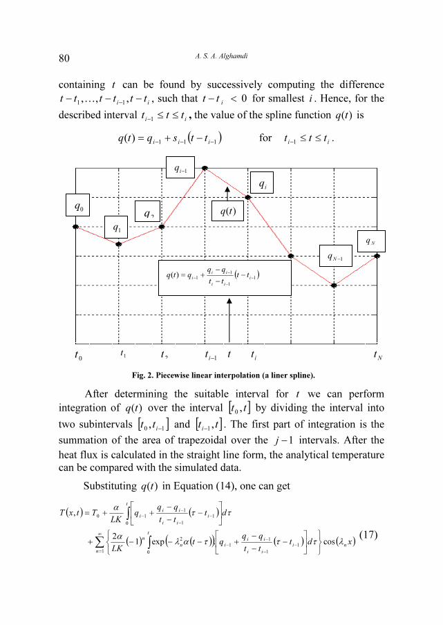
containing t can be found by successively computing the difference

iitttttt −−−

−

,,,11

… , such that 0<−itt for smallest i . Hence, for the

described interval iittt ≤≤

−1, the value of the spline function )(tq is

( )111

)(−−−

−+=iiittsqtq for

iittt ≤≤

−1.

After determining the suitable interval for t we can perform

integration of )(tq over the interval [ ]tt ,0

by dividing the interval into

two subintervals [ ]10

,−i

tt and [ ]tti,

1−. The first part of integration is the

summation of the area of trapezoidal over the 1−j intervals. After the

heat flux is calculated in the straight line form, the analytical temperature

can be compared with the simulated data.

Substituting )(tq in Equation (14), one can get

( ) ( )

( ) ( )( ) ( ) ( )

cos.exp12

,

1

1

1

1

1

0

2

0

1

1

1

10

xdttt

qqqt

LK

dttt

qqq

LKTtxT

n

n

i

ii

ii

i

t

n

n

t

i

ii

ii

i

λττταλα

ττα

∑ ∫

∫

∞

=

−

−

−

−

−

−

−

−

⎭⎬⎫

⎩⎨⎧

⎥⎦

⎤⎢⎣

⎡−

−

−+−−−+

⎥⎦

⎤⎢⎣

⎡−

−

−++=

(17)

0t 1

t

2t t

1−it

it

Nt

Fig. 2. Piecewise linear interpolation (a liner spline).

0q

1q

iq

2q

1−iq

)(tq

Nq

( )1

1

1

1)(

−

−

−

−

−

−

−

+=i

ii

ii

itt

tt

qqqtq

1−Nq


Performing the integrations, the solution in terms of the piecewise

straight lines heat flux becomes

(18)

4.2 Finite Difference Solution

To check validation of the above solution (18), the direct problem

(1) can be solved using a finite difference method. The method will start

as follows:

Rewriting the partial differential equation in terms of finite

difference approximations to the derivatives

2

11

12

x

TTT

t

TTn

j

n

j

n

j

n

j

n

j

Δ

+−=

Δ

−−+

+

α (19)

Thus, if for certain n we know the values of n

jT for all j, ( initial

condition )()0,(0xTxT = ), we can solve the equation above to find

1+n

jT

for each j :

( ) ( ) ( ) n

j

n

j

n

j

n

j

n

j

n

j

n

j

n

jTFTTFTTT

x

tTT

0110112

1 212 −++=+−Δ

Δ+=

−+−+

+α

(20)

( )

( )( )

( ) ( )

( )

( )( )

( )( )

( )( ) ( )

( ) ( )( )

( )( )

( )

cos

,

x

e1tt

qq1

eq

1tt

tt

qqq

eett

qq1

ett

tt

qqq

ett

tt

qqq

1LK

2

tttt

qq

2

1ttq

ttqq2

1

LKTtxT

n1n

tt

1jj

1jj

22n

2n

tt

1j2n

1j1jj

1jj1j

1j

1i

tttt

1ii

1ii

22n

2n

tt

1i1ii

1ii1i

2n

tt

1i1ii

1ii1i

n

21j

1jj

1jj1j1j

1j

1i1ii1ii

0

1j2n

1j2n

1i2ni

2n

1i2n

i2n

λ

αλ

αλαλ

αλ

αλ

αλ

α

α

αλ

αλ

αλαλ

αλ

αλ

∑

∑

∑

∞

=

−−

−

−

−−

−−

−

−

−

−

=

−−−−

−

−

−−

−

−

−

−

−−

−

−

−

−

−

−

−

−−

−

=

−−

⎪⎪⎪⎪⎪⎪⎪⎪⎪⎪⎪

⎭

⎪⎪⎪⎪⎪⎪⎪⎪⎪⎪⎪

⎬

⎫

⎪⎪⎪⎪⎪⎪⎪⎪⎪⎪⎪

⎩

⎪⎪⎪⎪⎪⎪⎪⎪⎪⎪⎪

⎨

⎧

⎟⎟⎟⎟⎟⎟⎟⎟⎟⎟⎟⎟⎟⎟⎟⎟⎟⎟⎟⎟⎟⎟

⎠

⎞

⎜⎜⎜⎜⎜⎜⎜⎜⎜⎜⎜⎜⎜⎜⎜⎜⎜⎜⎜⎜⎜⎜

⎝

⎛

⎟⎟⎟

⎠

⎞

⎜⎜⎜

⎝

⎛

⎟⎟⎠

⎞⎜⎜⎝

⎛−

−

−−

−⎟⎟

⎠

⎞

⎜⎜

⎝

⎛−

−

−++

⎥⎥⎥⎥⎥⎥⎥⎥⎥⎥⎥

⎦

⎤

⎢⎢⎢⎢⎢⎢⎢⎢⎢⎢⎢

⎣

⎡

⎟⎟⎟

⎠

⎞

⎜⎜⎜

⎝

⎛

⎟⎠

⎞⎜⎝

⎛−

−

−−

⎟⎟⎠

⎞⎜⎜⎝

⎛−

−

−+−

⎟⎟⎠

⎞⎜⎜⎝

⎛−

−

−+

−+

⎪⎪

⎭

⎪⎪

⎬

⎫

⎪⎪

⎩

⎪⎪

⎨

⎧

−−

−+−+

⎥⎦

⎤⎢⎣

⎡−+

+=

−

−

−

−


where

Equation for the left boundary condition 0),0(=

∂

∂

x

tT:

[ ] n

j

n

j

n

j

n

j

n

jTFTTTFT

010

141]2[ −+++=

−

+

(21)

[ ] n

j

n

j

n

jTFTFT

010

121]2[ −+=

−

+ (22)

[ ] nnn

TFTFT2030

1

2212 −+=

+ (23)

Equation for the right boundary condition )(),(

tqx

tLTk =

∂

∂

( )t

TTxcTTh

x

TTk

n

j

n

jn

j

n

j

n

j

Δ

−Δ=−+

Δ

+

∞

−

1

1

2

_ρ (24)

t

TTxctq

x

TTk

n

j

n

jn

n

j

n

j

Δ

−Δ=+

Δ

+

+−

1

11

2)(

_ρ (25)

Rearranging the above equation, we get

⎥⎦

⎤⎢⎣

⎡ Δ+⎟⎟

⎠

⎞⎜⎜⎝

⎛+= +

−

+ )(21

2 1

0

10

1 nn

j

n

j

n

jtq

k

xT

FTFT (26)

where c

k

ρα = ,

20

x

tF

Δ

Δ=α

For stability purposes, we must have the following condition in the

Fourier number

( ) 2

1

20≤

Δ

Δ=

x

tF

α

(27)

A finite difference program was written to compare numerical and

analytical solutions for )()( tftq = . The temperature profile for both

analytical and finite difference solutions was compared in Fig. 3. From

analysis of Fig. 3 it follows that both solutions yield the same results.

2T

3T

1T


4.3 MATLAB Code

The Levenberg-Marquardt method is used to solve the inverse

problem. It is an efficient method for solving linear problems that are ill-

conditioned [17,18]

. For the solution of the present inverse problem, we

consider the unknown heat flux )(tq to be expressed as linear spline

function in t , i.e., as a piecewise straight line representation, with

unknown parameters i

q .

The solution of the heat conduction problem (2) with )(tq

unknown parameterized as piecewise straight line function is an inverse

heat conduction problem in which the parameters i

q are to be estimated

in equation (18). The solution of this inverse heat conduction problem for

the estimation of the N unknown parameters i

q , for ,,...,2,1 Ni = is

based on the minimization of the ordinary least squares norm:

2

1

)()( ∑ ⎥⎦

⎤⎢⎣

⎡−=

=

∗I

i

ii qTTqS (28)

Fig. 3. Comparison between the analytical and the finite difference solutions for heat flux 2

0)( tqtq =

.

0 10 20 30

0

50

100

150

200

250

300

350

400

time (s)

T (o

C)

Temperature evolut ion at x=0

Tanl

Tfd

0 10 20 300

100

200

300

400

time (s)

T (o

C)

Temperature evolution at x=L/2

Tanl

Tfd

0 10 20 300

100

200

300

400

time (s)

T (o

C)

Temperature evolut ion at x=L

Tanl

Tfd


where

S = sum of squares error or objective function

[ ]N

Tqqqq ,...,,

21≡ = vector of unknown parameters

( ) ( )iitqTqT ,≡ = estimated temperature at time

it

( )i

i tTT

∗∗

≡ = measured temperature at it

N = total number of the unknown parameters

I =total number of measurements, where NI ≥

The estimated temperatures ( )qTi

are obtained from the solution of

the direct problem at the measurement location, measx , by using the

estimated unknown parameters i

q , Ni ,...,2,1= . The unknown vector

[ ]N

Tqqqq ,...,,

21≡ is determined by minimizing )(qS using the iterative

procedure in the Levenberg-Marquardt method [17, 18]

.

After defining the direct and inverse formulations, the Matlab code

is written to solve the inverse problem with the help of optimization tool

box [19]

which impelements the criteria, and the Levenberg-Marquardt

method. The iterative procedure, the stopping criteria, and the

computational algorithm were chosen based on the Levenberg-Marquardt

Matlab function capability.

5. Test Cases: Inverse Solution for Known Heat Flux Profile

In this section, two test cases are discussed. One test case is for a

heat flux that increases in a linear fashion at time. Exact values of the

simulated temperature history are used. The second case is for a heat flux

which varies at time in a triangular fashion; for this case both exact

temperatures and temperatures with random errors are used.

For the time interval 1200 ≤< t , we consider 100 transient

measurements of a single sensor located at 0=measx .

5.1 Simulated Measurements

Simulated measurements are obtained from the solution of the

direct problem at sensor location by using prior prescribed values for the

unknown parameters i

q of heat flux )(tq .


For example, if we consider that we can represent the heat flux

with 10 parameters, i.e.,

( )1

1

1

1)(

−

−

−

−

−

−

−

+=i

ii

ii

itt

tt

qqqtq ,

with ],,,[1021qqqq …= at

1021,...,, tttt

i= , for 10=N .

By using the known heat flux described above, the solution (18) of the

direct problem at the measurement location 0=measx provides the exact

(errorless) measurements )(*

iex tT , for Ii ,,1…= . Measurements

containing random errors are simulated by adding an error term to

)(*

iex tT in the form

[1]

ϖσ+= )()(**

iexi tTtT (29)

where

)(*

itT = simulated measurements containing random errors

)(*

iex tT = exact (errorless) simulated measurements

σ = standard deviation of the measurements errors

ϖ = random variable with normal distribution, zero mean and

unitary standard deviation, for the %99 confidence level we

have 576.2576.2 <<− ϖ .

With use of such simulated measurements as the input data for the

inverse analysis, we expect the code to return the same values of

parameters used to find the direct solution.

5.2 Case One: Linear Increase in Heat Flux

The surface heat flux )(tq increases linearly in time in the form

tqtq0

)( = over the interval ftt ≤<0 . The results of the inverse

calculation for case 0=σ are shown in Fig. 4. A comparison of the

exact simulated and estimated values of the temperatures profile at

insulated surface of probe shown in the figure reveals that they are in

excellent agreement. Also, it is clear from the figure the recovered heat

flux coincides with the exact heat flux. To test the code accuracy, a

simulated measurement containing random errors was used. Figure 5

compares the heat flux profiles for both cases to the exact profile, a


satisfactory result for the case of perturbed measurements is achieved.

The results obtained in the figure show that increasing the measurement

errors decrease the accuracy of the inverse algorithm.

Fig. 4. Results from IHCP algorithm using time-varying heat flux in the form tqtq0

)( =

.

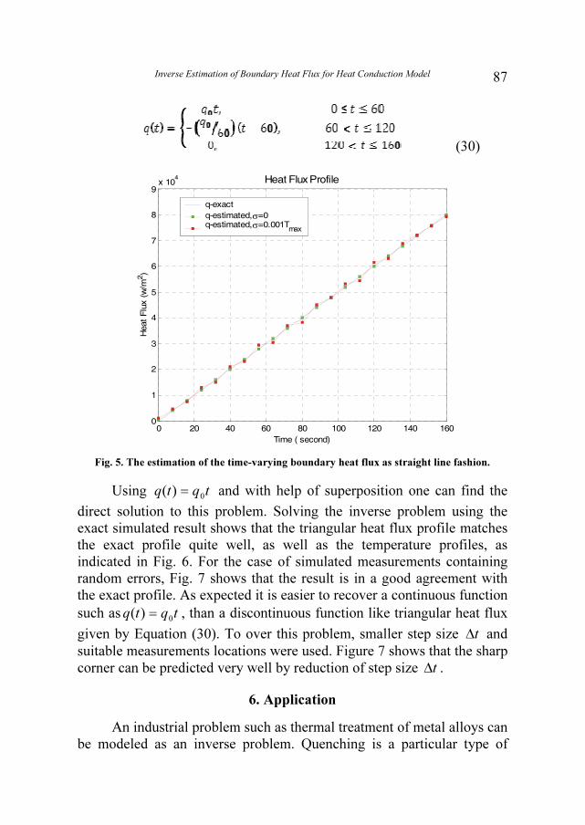
5.3 Case Two: Triangular Heat Flux

In this case the heat flux varies in time in a triangular fashion. To

form the heat flux profile, we let the surface heat flux )(tq increases

linearly with time for t between zero and 60, and for 60>t the flux

decreases linearly to zero at 120=t and remains zero thereafter.

Mathematically, it is in the form:

0 50 100 150 2000

100

200

300

400

500

600

Time ( s)

Te

mp

era

ture

(oC

)

Exact Simulated Temperature

0 50 100 150 2000

100

200

300

400

500

600

Time ( s)

Te

mp

era

ture

(oC

)

Analytical Profile Results

0 50 100 150 2000

100

200

300

400

500

600

Time ( s)

Te

mp

era

ture

(oC

)

Comparison of Simulated and Analy tical Results

0 50 100 150 2000

2

4

6

8

10x 10

4

Time ( s)

Heat F

lux

(w

/m2)

Heat Flux Prof ile

T-exp

T-anl

q-exact

q-anl,σ=0


0 20 40 60 80 100 120 140 1600

1

2

3

4

5

6

7

8

9x 10

4

Time ( second)

Heat

Flu

x (

w/m

2)

Heat Flux Profile

q-exact

q-estimated,σ=0q-estimated,σ=0.001T

max

(30)

Fig. 5. The estimation of the time-varying boundary heat flux as straight line fashion.

Using tqtq0

)( = and with help of superposition one can find the

direct solution to this problem. Solving the inverse problem using the

exact simulated result shows that the triangular heat flux profile matches

the exact profile quite well, as well as the temperature profiles, as

indicated in Fig. 6. For the case of simulated measurements containing

random errors, Fig. 7 shows that the result is in a good agreement with

the exact profile. As expected it is easier to recover a continuous function

such as tqtq0

)( = , than a discontinuous function like triangular heat flux

given by Equation (30). To over this problem, smaller step size tΔ and

suitable measurements locations were used. Figure 7 shows that the sharp

corner can be predicted very well by reduction of step size tΔ .

6. Application

An industrial problem such as thermal treatment of metal alloys can

be modeled as an inverse problem. Quenching is a particular type of


thermal treatment process that involves rapid cooling of metal alloys for

the purpose of hardening. Experimental measurements of temperature

history of quenching experiments can be used to determine the surface

heat fluxes. The developed model was used to estimate the heat flux for

the quenching experiment developed at Ohio University [20]

. The

developed algorithm was used to solve this problem [15]

, but for the sake

of completeness, the description of the experiments and the results will

be presented.

Fig. 6. Results from IHCP algorithm using time-varying heat flux in the form of triangular

function.

0 50 100 150 2000

50

100

150

200

Time ( s)

Te

mp

era

ture

(oC

)

Exact Simulated Temperature

0 50 100 150 2000

50

100

150

200

Time ( s)

Te

mp

era

ture

(oC

)


0 50 100 150 2000

50

100

150

200

Time ( s)

Te

mp

era

ture

(oC

)

Comparison of Simulated and Analy tical Results

T-exp

T-anl

0 50 100 150 200-0.5

0

0.5

1

1.5

2

2.5

3

3.5x 10

4

Time ( s)

He

at

Flu

x (

w/m

2)

Heat Flux Profile

q-exact

q-anl,σ=0


0 20 40 60 80 100 120 140 160-0.5

0

0.5

1

1.5

2

2.5

3

3.5x 10

4

Time ( second)

Heat

Flu

x (

w/m

2)

Heat Flux Profile

q-exact

q-estimated,σ=0q-estimated, σ=0.001T

max

Fig. 7. The estimation of the time-varying boundary heat flux as triangular function fashion.

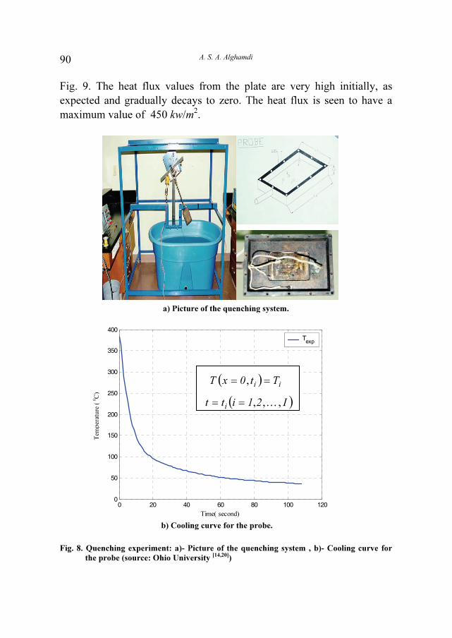
Experiments were conducted with a stainless steel probe in the

shape of a rectangular box as shown in Fig. 8a. The sides of the box are

approximated by, with each wall thick [20]

. The experimental

results of temperature data versus time is given in Fig. 8b for the

thermocouple which is attached to the inside surface (at the center) of the

wall of the probe. Since the wall thickness is much smaller than

the wall dimensions, the one-dimensional solution is valid for this wall of

the probe. The temperature data collected from the quench probe is

shown in Fig. 8b. The period corresponds to the air cooling of the probe

during transport from oven to the quenching oven is removed.

Results from IHCP algorithm are presented in Fig. 9. In order to

improve the accuracy of algorithm, the time step is significantly reduced.

The experimental and analytical temperatures are compared in Fig. 9. It

can be seen that the two temperature profiles match quite well. This

indicates that the inverse solution is accurate, and it can be used to find

the heat flux. Based on the analytical profile, the heat flux is then

estimated based on Equations (18) and (28). The results are also shown in


Fig. 9. The heat flux values from the plate are very high initially, as

expected and gradually decays to zero. The heat flux is seen to have a

maximum value of 450 kw/m2.

a) Picture of the quenching system.

b) Cooling curve for the probe.

Fig. 8. Quenching experiment: a)- Picture of the quenching system , b)- Cooling curve for

the probe (source: Ohio University [14,20]

)

0 20 40 60 80 100 1200

50

100

150

200

250

300

350

400

Time( second)

Tem

peratuer(0c)

Expermental profile result

Texp

( )ii

Tt0xT == ,

( )I21itti

,,, …==

Tem

per

atu

re (

0C

)


Fig. 9. Results from IHCP algorithm using experimental data from quench probe

[15].

Previous studies of this inverse heat conduction problem, which

included the 6th

degree polynomial and cubic spline, have some

limitations [12,14]

. The cubic spline exhibits sensitivity of heat flux to

input data. When a cubic spline curve is used, the heat flux curve is

assumed to be smooth so that the first derivative is continuous at the

interface between the intervals. Consequentially, this requirement

produces variations in the heat flux curve similar to sinusoidal curves.

Using a piecewise continuous straight line, on the other hand, does not

require a heat flux curve to be smooth. Therefore, in order to improve the

0 20 40 60 80 100 1200

100

200

300

400

Time ( s)

Te

mp

era

ture

(oC

)

Experimental Profile Result

Texp

0 20 40 60 80 100 1200

100

200

300

400

Time ( s)

Te

mp

era

ture

(oC

)


Tanl

0 20 40 60 80 100 1200

100

200

300

400

Time ( s)

Te

mp

era

ture

(oC

)

Comparison of Expermental and Analy tical Results

T-exp

T-anl

0 20 40 60 80 100 120-5

-4

-3

-2

-1

0

1x 10

5

Time ( s)

He

at

Flu

x (

w/m

2)

Heat Flux Profile

q(t)


stability of the solution, a piecewise continuous straight line

representation of )(tq has been used.

7. Conclusions

An analytical solution of the direct problem, which consists of

determining the temperature distribution in a one-dimensional uniform

plate for a given time-dependent heat flux boundary condition at one end

and the other end kept insulated, was developed for general form of heat

flux. The direct solution is determined by an approach based on the

method of variation of parameters. The solution is identical to the

solution found by Beck et al. [2]

for constant heat flux.

The analytical solution is developed based on a piecewise linear

representation of the heat flux and tested for different profiles. The

solution shows an excellent agreement with finite difference solution.

The piecewise linear interpolation model for heat flux is constructed to

be used in the inverse solution. The heat flux profile or values were then

found by employing the Levenberg-Marquardt method to fit the

analytical solution based on simulated data. Then the analytical solution

of the temperature profile over the plate is found based on this heat flux.

Comparing temperatures history calculated by the inverse algorithm with

that found by using known heat flux profile (simulated data) shows that

the two solutions are in excellent agreement.

As an industrial problem, the algorithm was applied to

experimental data obtained from a quenching experiment developed at

Ohio University. The heat flux history during the quenching process is

found and the theoretical temperature curve obtained from the analytical

solution is compared with experimental results. The two temperature

solutions show very satisfactory agreement [15]

.

Nomenclature

Acronyms

IHCP Inverse heat conduction problem

English Symbols

k thermal conductivity [ KmW .

]

L thickness of plate [m]

q heat flux [ 2mW ]


S sum of squares error or objective function [-]

T temperature [ C0 ]

t time [s]

x space coordinate [m]

u temperature [ C0

]

N total number of the unknown parameters [-]

I total number of measurements [-]

Greek Symbols

α thermal diffusivity [ sm2 ]

v temperature [ C0

]

λ eigenvalues [-]

τ dummy variable [-]

ζ dummy variable [-]

Subscripts

i integer (for temperatures measurements)

n integer ( for eigenvalues)

0 initial temperature

f final reading of temperature ( final time)

meas measured temperature at interior point of the probe

Superscripts

∗ measured temperature at it

n integer ( for eigenvalues)

T transpose

References

[1] Ozisik, M. N. and Orlande, R. B. H., Inverse Heat Transfer, Taylor and Francis, New

York ( 2000).

[2] Beck, J. V., Blackwell, B. and St. Clair, C. R., Inverse Heat Conduction, III Posed

Problems, A Wiley Interscience Publication, New York (1985).

[3] Beck, J., Blackwell, V. B. and Sheikh-Haji, A., Comparison of Some Inverse Heat

Condition Methods Using Experimental Data, Int. J. Heat Mass Transfer, 39(17): 3649-

3657 (1996).

[4] Taler, J. and Duda, P., Solving Direct and Inverse Heat Conduction Problems, Springer,

Berlin (2006).

[5] Tervola, P., A Method to Determine the Thermal Conductivity from Measured Temperature

Profiles, Int. J. Heat Mass Transfer, 32:1425-1430 (1989).

[6] Lesnic, D., Elliott, L. and Ingham, D. B., The Solution of an Inverse Heat Conduction

Problem Subject to the Specification of Energies", Int. J. Heat Mass Transfer, 41: 25-32

(1998).


[7] Tseng, A. A., Chang, J. G., Raudensky, M. and Horsky, J., An Inverse Finite Element

Evaluation of Roll Cooling in Hot Rolling of Steels, Journal of Material Processing and

Manufacture Science, 3: 387-408 (1995).

[8] Huang, C. H., Ju, T. M. and Tseng, A. A., The Estimation of Surface Thermal Behavior of

the Working Roll in Hot Rolling Process, Int. J. Heat Mass Transfer, 38: 1019-1031 (1995).

[9] Keanini, R. G., Inverse Estimation of Surface Heat Flux Distributions During High Speed

Rolling Using Remote Thermal Measurements, Int. J. Heat Mass Transfer, 41: 275-285

(1998).

[10] S. Abboudi, E. Artiouknine and H. Riad, Computational and Experimental Estimation of

Boundary Conditions for a Flat Specimen, Preliminary program inverse problems in

engineering iii, Port Ludlow Resort & Conference Center, 200 Olympic Place, Port Ludlow,

WA 98365 (1999).

[11] Stolz, G., Jr., Numerical Solutions to an Inverse Problem of Heat Conduction for Simple

Shapes, J. Heat Transfer, 82:20-26 (1960).

[12] Alam, M. K., Pasic, H., Anugarthi, K. and Zhong, R., Determination of Surface Heat Flux

in Quenching, ASME IMECE Proceedings, Nashville, November (1999).

[13] Kumar, Analytical Solution for Inverse Heat Conduction Problem, M.S. Thesis, Ohio

University (1998).

[14] Zhong, R., Inverse Algorithm for Determination of Heat Flux, M.S. Thesis, Ohio University

(1999).

[15] Alghamdi, A. S. A., and Alam, M. K., Inverse heat transfer solution for the flat plate probe,

Proceedings of the 3rd BSME-ASME International Conference on Thermal Engineering,

Dhaka, Bangladesh (2006).

[16] Poulikakos, D., Conduction Heat Transfer, Prentice-Hall, Inc (1994).

[17] Levenberg, K., A Method for the Solution of Certain Non-linear Problems in Least

Squares, Quart. Appl. Math., 2:164-168 (1944).

[18] Mrquardt, D. W., An Algorithm for Least Squares Estimation of Nonlinear Parameters, J.

Soc. Ind. Appl. Math, 11: 431-441 (1963).

[19] Chong, K. P. E. and Zak, H. S., An Introduction to Optimization, Prentice-Hall, Inc (1996).

[20] Zajc, D., Experimental Study of a Quench Process, M.S. Thesis, Ohio University (1998).


��

��

��

��: �� !� "#�!$� %�&�' (�' ��

)�*�!�� +� �,�� -�� ./� .�$� �0 . #�� (�23 �� #0�( 4�� 5�2�( +!�� (�26� 7�0 -��

8&�9� -��5�� :;�0� <=�& >�� (��$� <=�&� . ��$�� -�� #� �� #�� (�23 *� :(?�� *��

(IHCP)� <��( -' .�/� *�!�� 4�,� .�� , #A�� <�� +&=� #�� &0 �� -�� ./�� . #��

��$�� -�� >�� (��$� <�� <�!��0 �� <=�&Levenberg-Marquardt .<��$�� <�!��0�� B=�� (C�� D��26�4(�( ��(0�� E�� 5��0� <��$� #��

-�� ./�� . �(=�� -�� ./�� *� < ��=�� 5�?F' (C�5�� +�2� <�� <2� :��$�� . E�� (0��

�� -�� ./�� (=� �� G��0� ($�� -�� -�� ' <$��2 ��.

inverse estimation of boundary heat flux for heat ...model for heat flux is used. the inverse...

Documents