INVERSE KINEMATICS AND GEOMETRIC CONSTRAINTS

FOR ARTICULATED FIGURE MANIPULATION

by

Chris Welman

B�Sc� Simon Fraser University ����

a thesis submitted in partial fulfillment

of the requirements for the degree of

Master of Science

in the School

of

Computing Science

c� Chris Welman ����

SIMON FRASER UNIVERSITY

September ����

All rights reserved� This work may not be

reproduced in whole or in part� by photocopy

or other means� without the permission of the author�

APPROVAL

Name� Chris Welman

Degree� Master of Science

Title of thesis� Inverse Kinematics and Geometric Constraints for Articulated Fig�

ure Manipulation

Examining Committee� Dr� L� Hafer

Chair

Dr� T�W� Calvert

Senior Supervisor

Dr� J� Dill

Dr� D� Forsey

External Examiner

Date Approved�

ii

Abstract

Computer animation of articulated �gures can be tedious� largely due to the amount of data which

must be speci�ed at each frame� Animation techniques range from simple interpolation between

keyframed �gure poses to higher�level algorithmic models of speci�c movement patterns� The former

provides the animator with complete control over the movement� whereas the latter may provide

only limited control via some high�level parameters incorporated into the model� Inverse kinematic

techniques adopted from the robotics literature have the potential to relieve the animator of detailed

speci�cation of every motion parameter within a �gure� while retaining complete control over the

movement� if desired�

This work investigates the use of inverse kinematics and simple geometric constraints as tools

for the animator� Previous applications of inverse kinematic algorithms to computer animation are

reviewed� A pair of alternative algorithms suitable for a direct manipulation interface are presented

and qualitatively compared� Application of these algorithms to enforce simple geometric constraints

on a �gure during interactive manipulation is discussed� An implementation of one of these algo�

rithms within an existing �gure animation editor is described� which provides constrained inverse

kinematic �gure manipulation for the creation of keyframes�

Contents

� Introduction �

��� Organization � � � � � � � � � � � � � � � � � � � � � � � � � � � � � � � � � � � � � � � �

� Approaches to Figure Animation �

�� Body Models � � � � � � � � � � � � � � � � � � � � � � � � � � � � � � � � � � � � � � � � �

���� Scope � � � � � � � � � � � � � � � � � � � � � � � � � � � � � � � � � � � � � � � � �

��� Skeleton Modelling � � � � � � � � � � � � � � � � � � � � � � � � � � � � � � � � �

� Kinematic Methods � � � � � � � � � � � � � � � � � � � � � � � � � � � � � � � � � � � � � �

��� Forward Kinematics � � � � � � � � � � � � � � � � � � � � � � � � � � � � � � � � �

�� Inverse Kinematics � � � � � � � � � � � � � � � � � � � � � � � � � � � � � � � � � �

�� Dynamic Methods � � � � � � � � � � � � � � � � � � � � � � � � � � � � � � � � � � � � � �

���� Forward Dynamics � � � � � � � � � � � � � � � � � � � � � � � � � � � � � � � � � �

��� Inverse Dynamics � � � � � � � � � � � � � � � � � � � � � � � � � � � � � � � � � � ��

� Control Issues � � � � � � � � � � � � � � � � � � � � � � � � � � � � � � � � � � � � � � � � �

�� Summary � � � � � � � � � � � � � � � � � � � � � � � � � � � � � � � � � � � � � � � � � � ��

� Inverse Kinematics ��

��� The Inverse Kinematic Problem � � � � � � � � � � � � � � � � � � � � � � � � � � � � � � �

�� Resolved Motion Rate Control � � � � � � � � � � � � � � � � � � � � � � � � � � � � � � ��

���� Redundancy � � � � � � � � � � � � � � � � � � � � � � � � � � � � � � � � � � � � � ��

��� Singularities � � � � � � � � � � � � � � � � � � � � � � � � � � � � � � � � � � � � � �

��� Optimization�Based Methods � � � � � � � � � � � � � � � � � � � � � � � � � � � � � � � �

����� Evaluation � � � � � � � � � � � � � � � � � � � � � � � � � � � � � � � � � � � � �

�� Applications to Computer Graphics � � � � � � � � � � � � � � � � � � � � � � � � � � � �

� E�cient Algorithms for Direct Manipulation ��

�� A Simpli�ed Dynamic Model � � � � � � � � � � � � � � � � � � � � � � � � � � � � � � �

���� The Jacobian Transpose Method � � � � � � � � � � � � � � � � � � � � � � � � � �

i

CONTENTS ii

��� Implementation Details � � � � � � � � � � � � � � � � � � � � � � � � � � � � � � ��

���� Computing the Jacobian � � � � � � � � � � � � � � � � � � � � � � � � � � � � � � ��

��� Scaling Considerations � � � � � � � � � � � � � � � � � � � � � � � � � � � � � � � ��

���� Integration � � � � � � � � � � � � � � � � � � � � � � � � � � � � � � � � � � � � � ��

���� Joint Limits � � � � � � � � � � � � � � � � � � � � � � � � � � � � � � � � � � � � � �

� A Complementary Heuristic Approach � � � � � � � � � � � � � � � � � � � � � � � � � � �

��� The Cyclic�Coordinate Descent Method � � � � � � � � � � � � � � � � � � � � � ��

�� Overview � � � � � � � � � � � � � � � � � � � � � � � � � � � � � � � � � � � � � � ��

�� Comparison � � � � � � � � � � � � � � � � � � � � � � � � � � � � � � � � � � � � � � � � � ��

� Incorporating Constraints ��

��� Constraint Satisfaction � � � � � � � � � � � � � � � � � � � � � � � � � � � � � � � � � � � �

�� Maintaining Constraints � � � � � � � � � � � � � � � � � � � � � � � � � � � � � � � � � �

���� The Constraint Condition � � � � � � � � � � � � � � � � � � � � � � � � � � � � � �

��� Computing the Constraint Jacobian Matrix � � � � � � � � � � � � � � � � � � � �

���� Computing the Constraint Force � � � � � � � � � � � � � � � � � � � � � � � � �

��� Solving for Lagrange Multipliers � � � � � � � � � � � � � � � � � � � � � � � � � �

���� Feedback � � � � � � � � � � � � � � � � � � � � � � � � � � � � � � � � � � � � � � �

���� Overview � � � � � � � � � � � � � � � � � � � � � � � � � � � � � � � � � � � � � � �

��� Implementation Issues � � � � � � � � � � � � � � � � � � � � � � � � � � � � � � � � � � � �

����� Skeletons as Objects � � � � � � � � � � � � � � � � � � � � � � � � � � � � � � � � �

���� Handles on Skeletons � � � � � � � � � � � � � � � � � � � � � � � � � � � � � � � � �

����� Constraints on Handles � � � � � � � � � � � � � � � � � � � � � � � � � � � � � � ��

���� The Global Picture � � � � � � � � � � � � � � � � � � � � � � � � � � � � � � � � � �

����� Summary � � � � � � � � � � � � � � � � � � � � � � � � � � � � � � � � � � � � � � �

�� A CCD�based Penalty Method � � � � � � � � � � � � � � � � � � � � � � � � � � � � � � �

An Interactive Editor �

��� A System Overview � � � � � � � � � � � � � � � � � � � � � � � � � � � � � � � � � � � � ��

����� Skeletons � � � � � � � � � � � � � � � � � � � � � � � � � � � � � � � � � � � � � � ��

���� The Sequence � � � � � � � � � � � � � � � � � � � � � � � � � � � � � � � � � � � � ��

����� The Editor � � � � � � � � � � � � � � � � � � � � � � � � � � � � � � � � � � � � � �

�� Direct Manipulation � � � � � � � � � � � � � � � � � � � � � � � � � � � � � � � � � � � � ��

��� Constraints � � � � � � � � � � � � � � � � � � � � � � � � � � � � � � � � � � � � � � � � � ��

� Conclusion

�� Summary � � � � � � � � � � � � � � � � � � � � � � � � � � � � � � � � � � � � � � � � � � ��

� Results � � � � � � � � � � � � � � � � � � � � � � � � � � � � � � � � � � � � � � � � � � � � �

CONTENTS iii

��� Comments about Constraints � � � � � � � � � � � � � � � � � � � � � � � � � � � �

�� Directions � � � � � � � � � � � � � � � � � � � � � � � � � � � � � � � � � � � � � � � � � �

Bibliography ��

List of Figures

�� �a� � objects de�ned in local coordinate systems� �b� Local rotations applied� �c�d�

Local translations applied� � � � � � � � � � � � � � � � � � � � � � � � � � � � � � � � � � �

��� Three con�gurations of a D redundant manipulator � � � � � � � � � � � � � � � � � � �

�� A manipulator in a singular con�guration � � � � � � � � � � � � � � � � � � � � � � � � �

�� Interactive control loop model for Jacobian transpose method � � � � � � � � � � � � � ��

� A case not handled well with the Jacobian transpose method� Pulling inwards on the

tip of the manipulator on the left will not produce an expected con�guration like the

one shown on the right� � � � � � � � � � � � � � � � � � � � � � � � � � � � � � � � � � � �

�� Example CCD iteration step for rotation joint i� � � � � � � � � � � � � � � � � � � � � ��

� � � � � � � � � � � � � � � � � � � � � � � � � � � � � � � � � � � � � � � � � � � � � � � � � �

�� � � � � � � � � � � � � � � � � � � � � � � � � � � � � � � � � � � � � � � � � � � � � � � � �

��� A force applied to a point constrained to lie within a plane� A constraining force

normal to the plane is added to the applied force to obtain a legal force tangential to

the plane� � � � � � � � � � � � � � � � � � � � � � � � � � � � � � � � � � � � � � � � � � � �

�� Iteration steps for maintaining constraints � � � � � � � � � � � � � � � � � � � � � � � � ��

��� A generic function block� � � � � � � � � � � � � � � � � � � � � � � � � � � � � � � � � � � ��

�� Example network� � � � � � � � � � � � � � � � � � � � � � � � � � � � � � � � � � � � � � ��

��� A branching chain with two end�e�ector constraints � � � � � � � � � � � � � � � � � � �

��� Sample skeleton description � � � � � � � � � � � � � � � � � � � � � � � � � � � � � � � � ��

�� Sequence editor screen � � � � � � � � � � � � � � � � � � � � � � � � � � � � � � � � � � � �

��� Plan view of goal determination in �a� an orthographic view� and �b� a perspective

view � � � � � � � � � � � � � � � � � � � � � � � � � � � � � � � � � � � � � � � � � � � � � ��

�� A �gure being positioned by �rst tilting� then twisting� the pelvis� � � � � � � � � � � �

��� �a� First keyframe pose �b� Interpolated pose �c� Second keyframe pose � � � � � � � ��

iv

Chapter �

Introduction

Computer graphics has advanced to a point where generating images of striking realism and com�

plexity has become almost commonplace� However� making objects move convincingly within these

pictures remains di�cult� particularly as object models grow increasingly complex� The speci�cation

and control of motion for computer animation has emerged as one of the principal areas of research

within the computer graphics community�

One area in particular which continues to receive attention is that of �gure animation� The goal

of work in this area is to provide a means of generating life�like� possibly human�like� articulated

�gures� and to design and control their actions within simulated environments� Animated human

�gures could� for example� be placed in simulated environments for ergonomic evaluation� or simply

to provide some aesthetic qualities to a presentation� In the arts and entertainment area� the concept

of computer�generated characters roaming through arti�cial worlds seems universally appealing�

Although �gure animation raises technical challenges in both modelling and rendering� the fun�

damental problem of designing and controlling movement for these �gures remains a particularly

di�cult one� Part of the problem lies in deciding from which level of detail to approach the task�

At one end of the scale� the movements of individual parts of the body must be known for each

instant in time� At the other end of the scale� coordinating movements and handling interaction

between �gures and with the environment may require algorithms based on behavioural rules and

knowledge bases� Many of the most impressive examples of �gure animation by computer have been

the result of algorithms implementing high�level behavioural and motor control models� However�

these algorithms are often limited to generating speci�c� usually repetitive� movement patterns such

as walking and running� For the animator who wishes to create new movements� there is little al�

ternative to painstakingly constructing the movement by hand� Given the complex structure of a

typical articulated �gure� this can involve an inordinate amount of work�

�

CHAPTER �� INTRODUCTION

The motivation behind this work is a desire to improve the animation capabilities of an existing

interactive articulated �gure animation package� which is currently used to create movements for

both dance and animation� It is shown how inverse kinematic techniques for controlling robotic

manipulators can be adopted to relieve the animator of some of the more tedious aspects of creating

new movements by hand� After reviewing the inverse kinematic problem and solutions that have

previously been applied to �gure animation� a pair of alternative solution algorithms are presented

and qualitatively compared� These algorithms are simple� yet e�ective� and can support both direct

manipulation of articulated �gures as well as the imposition of simple geometric constraints upon a

�gure� Implementations of these algorithms are presented� and are applied to develop a basic set of

interactive tools for �gure manipulation and animation�

��� Organization

Chapter reviews computer animation techniques in general� and discusses their applicability in

the context of �gure animation� In Chapter � the inverse kinematic problem is stated� and com�

mon approaches to solving the problem are reviewed� In Chapter a pair of fast� reliable inverse

kinematic algorithms are described� suitable for interactive manipulation tasks and di�ering from

previous algorithms adopted for computer graphics� In Chapter � procedures for satisfying simple

geometric constraints using these algorithms are considered� Chapter � introduces an interactive

�gure animation editor and discusses implementation of the algorithms as positioning aids�

Chapter �

Approaches to Figure Animation

Placing this work in context requires some understanding of computer animation techniques in

general� and of how they may be applied to �gure animation in particular� This chapter provides an

overview of the advantages and disadvantages of basic motion control techniques for �gure animation�

The emphasis here is on methods to create and control the movements of articulated �gures�

rather than simply replaying digitized movement� It is fair to say that for many productions� dig�

itizing� or rotoscoping � the movements of real subjects remains the method of choice for obtaining

convincing life�like motion� Rotoscoping can refer to techniques ranging from visually matching

graphic images to prerecorded video footage� to attaching some sort of sensors to a performer�s

body� whose positions can be tracked by computer and stored for later playback� Neither of these

are particularly attractive options� the former being quite tedious� and the latter relying on the

availability of reliable� unobtrusive instrumentation for the body� and sophisticated software to re�

construct the original motion from the sensor data� neither of which are readily available yet� A

further limitation of rotoscoping is that a �gure animated in this way is limited to those movements

actually performed by a live subject� Computer animation techniques can be applied to animate

�gures in situations for which rotoscoping is neither a viable nor practical solution�

��� Body Models

����� Scope

First we must decide exactly what we are trying to animate� Although the ideal computer�generated

�character� would include muscle and tissue that deforms during movement� skin and clothing that

wrinkles and stretches� hair that �ows� and expressive facial features� the accurate modelling� ani�

mation� and rendering of these attributes are research topics in their own right� and work in these

�

CHAPTER �� APPROACHES TO FIGURE ANIMATION

areas is still at the experimental stage� For the time being we will have to restrict our attention to

animating simple approximations to real bodies� It is useful to think of these simple approximations

as a skeletal layer� upon which muscle� tissue and skin can later be layered� The important point here

is that any body model can be animated by moving an underlying skeletal approximation� which

need not bear any resemblance to the �nal rendered appearance of the character� Thus the motion

control problem for �gures reduces to that of controlling the movement of an abstract articulated

skeleton�

����� Skeleton Modelling

A skeleton can be represented by a collection of simple rigid objects connected together by joints�

The joints are usually rotational� but may also be sliding �or prismatic�� Each rotary joint may

allow rotation in �� � or � orthogonal directions� these are the degrees of freedom �DOF� of the

joint� A detailed approximation to the human skeleton may have as many as �� degrees of freedom�

although often fewer su�ce� Restrictions on the allowable range of movements for a joint can be

approximated by limiting the rotation angle in each of the rotation directions at each joint�

The individual objects comprising the skeleton are each de�ned in their own local coordinate

systems� and are assembled into a recognizable �gure in a global world coordinate system by a

nested series of transformations� In Figure �� a simple articulated limb is built up by applying local

rotations and translations to blocks de�ned in their own local coordinate systems�

More complex skeletons can be built up by arranging the segments in a tree�structured hierarchy�

Each node in the tree maintains the rotations currently in e�ect at the corresponding joint� these

joint rotations are o�sets from the orientation of the parent segment in the tree� These nested

transformations in the hierarchy ensure that segments inherit the rotations applied to joints higher

in the tree� a rotation applied at� say� the shoulder joint� causes the entire arm to rotate� and not

just the upper arm segment� One joint in the skeleton needs to be speci�ed as the root of the tree�

transformations applied to this joint move the entire skeleton in the world coordinate system� The

choice of which joint is to serve as the root is irrelevant� and it is convenient to be able to restructure

an existing hierarchy around a new root joint at any time� The global transformations applied to

any particular object within the skeleton can be computed by traversing the hierarchy from the root

to the segment and concatenating the local transformations at each joint visited by the traversal�

Most animation systems provide a means of building up the transformation hierarchy needed to

de�ne a skeleton� and it is easy enough to de�ne a simple grammar for specifying skeletons �Zel�b��

Sims� �SZ��� has described an interactive editor for designing new skeletons which applies some

simple heuristics to streamline the process� Regardless of how it is created� a skeleton de�nition will

CHAPTER �� APPROACHES TO FIGURE ANIMATION �

(b)(a)

(c)(d)

Figure ��� �a� � objects de�ned in local coordinate systems� �b� Local rotations applied� �c�d� Localtranslations applied�

minimally specify the individual body segment lengths� the joint degrees of freedom� and the overall

hierarchy of the structure�

A skeleton can be animated by varying the local rotations applied at each joint over time� as well

as the global translation applied at the root joint� The motion speci�cation and control problem

is that of managing the way in which these transformations change over time� In general� there

are two fundamental approaches to this problem� kinematic and dynamic� The following sections

review both kinematic and dynamic methods for motion speci�cation in general� the types of control

available for each� and applications of these to �gure animation in particular�

��� Kinematic Methods

����� Forward Kinematics

Forward kinematics involves explicitly setting the position and orientation of objects at speci�c frame

times� For skeletons� this means directly setting the rotations at selected joints� and possibly the

global translation applied to the root joint� to create a pose� To avoid doing this for each frame

of an animation� a series of keyframe poses can be speci�ed at di�erent frames� with intermediate

CHAPTER �� APPROACHES TO FIGURE ANIMATION �

poses calculated by interpolating the joint parameters between the keyframes� The �gure can then

be animated by displaying each intermediate pose�

While linear interpolation between keyframes is the simplest method for generating these inter�

mediate poses� the resulting motion is usually unsatisfactory� Discontinuous �rst derivatives in the

interpolated joint angles at the keyframes lend a jerky� robotic quality to the motion� The use of

higher�order interpolation methods� such as piecewise splines� can provide continuous velocity and

acceleration� and hence smoother transitions between and through the keyframes� Keyframe inter�

polation is well established �Ste��� �Gom��� �HS��� �Sho��� �Stu� �� and is invariably provided in

commercial animation systems�

Controlling interpolation

Interpolation often produces intermediate values that do not quite meet the animator�s requirements�

some control over the interpolation process is crucial �Las� �� The interpolated values for a single

DOF over the course of an animation form a trajectory curve� which �usually� passes through the

keyframe values� The shape of the trajectory� and hence the motion of the object� is dependant on

both the keyframed values and the type of interpolating spline used� An interactive editor which

allows the animator to view and modify the shape of a trajectory can be a useful tool� Once a

trajectory is de�ned� the quality of the movement can be further modi�ed by varying the rate at

which the trajectory is traversed� A number of parameterized interpolation methods have been

proposed which provide varying degrees of control over both the shape of a trajectory and variations

in speed along the trajectory�

Kochanek �KB�� describes an interpolation technique based on a generalized form of piecewise

cubic Hermite splines� Three parameters � continuity � tension� and bias � are provided to control the

length and direction of vectors tangent to the trajectory at the keyframes� Modifying the direction

of the tangent vectors gives local control over the shape of the curve as it passes through a keyframe�

Changing the length of the tangent vectors a�ects the rate of change of the interpolated value around

the keyframe� and thus provides some control over speed� Some traditional animation e�ects such

as action follow�through and exaggeration �Las� � can be achieved with appropriate settings of these

parameters� Unfortunately� since all three parameters in the spline formulation a�ect the shape of

the curve� the method provides no means for modifying speed along a trajectory without modifying

the trajectory itself�

Steketee and Badler �SB��� advocate a double�interpolant method which does separate timing

control from the trajectory itself� As before� a trajectory is de�ned as a piecewise cubic spline passing

through a series of keyframed values� An additional spline curve is also introduced to control the

CHAPTER �� APPROACHES TO FIGURE ANIMATION

parameter with which the trajectory curve is sampled� This provides control over the parametric

speed at which the trajectory curve is traversed� However� there is often no meaningful relationship

between parametric speed and actual speed in the geometric sense� sampling a curve at uniformly

spaced parametric points will not necessarily yield uniformly spaced points in space� This approach

to timing adjustment� therefore� is somewhat ad hoc and non�intuitive� requiring a trial�and�error

process on the part of the animator to achieve the desired velocity pro�le along the trajectory�

More intuitive control over speed along a trajectory can be obtained by reparameterizing the

trajectory curve by arc�length� Arc�length parameterization provides a direct relationship between

parametric speed and geometric speed along a trajectory� the distance �d travelled along a trajectory

is proportional to the increment �s of the trajectory�s arc�length parameter s� Allowing the animator

to sketch a curve representing s over time provides an intuitive mechanism for varying speed along

the trajectory �BH���� However� although theoretically a reparameterization by arc�length exists for

any curve� it is often not possible to �nd an analytic solution for arbitrary curves� and one must

resort to numerical approximation methods �Gir��� �GP����

Evaluation

Keyframe�based computer animation has a direct analogy in traditional animation� where key ani�

mation cels are drawn by senior animators� while less experienced animators draw the action in the

intermediate cels� Computer�based keyframing is intuitive� and the interpolation can usually be per�

formed fast enough to provide near real�time feedback� For skeleton animation� however� keyframe

interpolation does not work well� the few good examples of keyframed �gure animation are more a

tribute to the skill and patience of the animator than to the technique�s suitability for the task�

One major di�culty can be labelled the �degrees of freedom� problem� for interesting skeletons�

there are simply too many DOFs for which values must be provided� the level of detail required

from the animator to specify even a single key pose is excessive� Trying to control the interpolated

motion by manually modifying possibly hundreds of trajectory curves can be tedious� frustrating

and error�prone� While it is essential that the animator have some control at the joint level� higher

levels of control are desirable for specifying the coordinated movements of groups of joints�

Even supposing that the number of degrees of freedom within a �gure is manageable� the common

practice of displaying interpolated joint angles as a set of three splined trajectory curves � is rarely

helpful� Unlike translations� an ordered series of rotations do not combine intuitively� making it

di�cult to predict the consequences of editing a single rotation trajectory and almost impossible to

decide on the appropriate changes to all three curves which will produce a desired change in a single

�one each for the X�Y� and Z rotation directions at each joint

CHAPTER �� APPROACHES TO FIGURE ANIMATION �

body segment�s motion�

The hierarchical structure of the skeleton also causes problems� The only joint which an animator

can explicitly position is the root joint in the hierarchy� the positions of all other objects in the

skeleton depend on the rotations at ancestor joints� This makes it di�cult to enforce positional

constraints when creating a keyframe pose� For example� if the hierarchy root for a biped is at the

pelvis� then placing a foot on the �oor and keeping it there is troublesome� if the foot is already in

place� then a bend at the knee will move the foot� which must then be repositioned by modifying

the rotation at the hip joint� The ability to rearrange the hierarchy about a new root joint is only

marginally useful� In our example� making the support foot the new root of the hierarchy would

allow a knee bend which leaves the foot in place� However� this will also move the rest of the body�

which may move another� previously positioned body segment� such as the other foot� This makes

enforcing multiple positional constraints a frustrating process�

The same problem crops up during interpolation� Even if an animator has made sure that

both feet are positioned correctly in a series of keyframe poses� there is no guarantee that simply

interpolating joint rotations will maintain the correct foot positions at the intermediate frames�

It is quite common to see interpolated keyframed sequences for �gures in which the feet seem to

penetrate through� or slide around on� the �oor� While this can be remedied by specifying additional

keyframes� as the keyframe spacing becomes smaller the animation process begins to resemble the

frame�by�frame positioning of traditional stop�action animation �claymation� for example�� This

defeats the whole purpose of interpolation� which is intended to relieve the animator from the tedium

of specifying the motion on a frame�by�frame basis�

While forward kinematics combined with a simple interpolation scheme may su�ce for animating

simple objects� it is not really up to the task of animating articulated �gures�

����� Inverse Kinematics

Using forward kinematics� the position of any object within a skeleton can only be indirectly con�

trolled by specifying rotations at the joints between the root and the object itself� In contrast�

inverse kinematic techniques provide direct control over the placement of an end�e�ector object at

the end of a kinematic chain of joints� solving for the joint rotations which place the object at the

desired location� In light of the preceeding discussion� it should be apparent that inverse kinematics

o�ers an attractive alternative to explicitly rotating individual joints within a skeleton� An animator

can instead directly specify the position of an end�e�ector� while the system automatically computes

the joint angles needed to place the part� Not surprisingly� the inverse kinematic problem has been

studied extensively in the robotics �eld� although it is only fairly recently that the techniques have

CHAPTER �� APPROACHES TO FIGURE ANIMATION �

been adopted for computer animation�

Chadwick�s Critter system permits inverse kinematic manipulation of a skeleton for creating

keyframes �CHP���� Badler has proposed an inverse kinematic algorithm to enforce positional con�

straints on multiple body parts during skeleton manipulation �BMW� �� and has incorporated joint

range limits into the inverse kinematic solution �CP��� ZB���� Both Girard�s PODA system �GM���

and Sims� gait controller �SZ��� provided high�level locomotion models for skeletons� using inverse

kinematics to generate the leg motion� In these systems� a planning stage determines foot place�

ments and trajectories� while the inverse kinematic algorithm is responsible for generating the leg

joint angles as the feet are moved along trajectories between each foot�hold�

Inverse kinematics provides higher�level control over joint hierarchies than simple forward kine�

matics� moving the limbs of a skeleton becomes much more manageable� However� often the un�

derlying method for generating motion still relies on strictly kinematic methods� Unfortunately�

kinematic methods do not produce convincing movement without a considerable amount of e�ort

on the animator�s part� Often� the motion exhibits a weightless quality which is di�cult to dispel

by editing the trajectories and timing for individual degrees of freedom� Kinematic methods� both

forward and inverse� do not produce movement with the sort of dynamic integrity we have come to

expect from our experience with the physical laws of the real world�

��� Dynamic Methods

Animation based on dynamic simulation is attractive because the generated motion adheres to phys�

ical laws� providing a level of realism that is extremely di�cult to duplicate with kinematic methods�

For dynamic analysis� object descriptions must include such physical attributes as the center of mass�

the total mass� and the moments and products of inertia� Although there are many formulations for

the equations of motion� they are all essentially equivalent to the familiar F � ma� which relates the

acceleration a an object of mass m undergoes in response to a force F applied at the object�s center

of mass �� The motion generated by physical simulation is controlled by the application of forces

and torques� which may vary over time� Techniques for dynamic motion control can be categorized

as either forward dynamic methods or inverse dynamic methods� The essential distinction between

the two is in the way that the basic forces and torques driving the motion are arrived at�

����� Forward Dynamics

Forward dynamics involves explicit application of time�varying forces and torques to objects� Some

forces� such as those due to gravity and collisions between objects� may be handled automatically

�a similar equation relates angular acceleration to applied torques

CHAPTER �� APPROACHES TO FIGURE ANIMATION ��

by the animation system� other forces are applied directly by the animator to objects in the scene�

The motion is approximated by taking a series of discrete steps in time� and at each step solving the

equations of motion for the acceleration an object undergoes in response to the applied forces� Given

the position and velocity of an object from the previous time step� the acceleration a can be twice

integrated to determine a new velocity and position� respectively� for the current time step� A good

introduction and overview of the basics of forward dynamic simulation for animating rigid bodies

can be found in �Wil���� A comprehensive approach to simulating the motion of rigid polyhedral

objects� accounting for collisions� is presented by Hahn �Hah����

Extending this approach to the simulation of articulated skeletons is challenging� In general�

there will be one equation of motion for each degree of freedom in the skeleton� This leads to a large

system of equations� which must be solved by numerical methods at considerable computational

expense� The formulation adopted to represent the equations of motion signi�cantly a�ects the cost

of the solution method� A solution for the matrix�based Gibbs�Appell formulation� for example�

has O�n�� complexity for n degrees of freedom �Wil� �� Armstrong has proposed an alternative

recursive formulation which reduces the complexity to O�n� �AG���� enabling dynamic simulations

of simple articulated structures to be performed in close to real�time� But dynamic simulation of

reasonably complex articulated skeletons cannot in general be performed at interactive speeds on

single�processor machines� although the recursive formulation may be fast enough to be tolerable�

Complicating matters is the fact that the equations of motion for articulated skeletons are con�

siderably more complex than those for simple objects� since they must include terms to model the

interactions between connected body parts� This coupling of the dynamics equations makes control

extrememly di�cult� since movement of one segment of the skeleton will exert forces and torques

on adjacent segments� the notion that the motion of the skeleton can be adequately controlled by

applying joint torques individually is incorrect �Wil���� E�orts to counteract this unwanted prop�

agation of torques usually involve placing springs and dampers at each joint to maintain a desired

orientation� Unfortunately� this type of control invariably leads to a sti� set of equations� which

causes severe instability in most numerical solution techniques� A summary of numerical stability

and control issues that must be addressed during dynamic simulation is presented in �Gir����

Compounding the problem of numerical instabilities is the fact that the equations of motion for

articulated skeletons are inherently ill�conditioned� independent of their formulation �Mac���� The

ill�conditioning arises when the skeleton assumes a posture in which small incremental changes in

one degree of freedom produce large accelerations elsewhere� almost all numerical solution techniques

have di�culty handling such cases� Maciejewski contends that these situations occur frequently for

articulated �gures� and are inherent in the structure of most skeletons� The ill�conditioning of the

CHAPTER �� APPROACHES TO FIGURE ANIMATION ��

equations has implications not only for dynamic analysis� but inverse kinematic algorithms as well�

�Mac��� gives a lucid description of the problem� and discusses methods for detecting and handling

the ill�conditioning in both cases�

One of the earliest attempts to control an articulated �gure purely through forward dynamic

simulation was Wilhelms� V irya system �Wil���� V irya permitted the interactive design of force or

torque versus time functions for individual degrees of freedom� Force and torque keyframes could be

speci�ed at di�erent times� cubic splines were then used to construct the force and torque pro�les over

the course of the entire motion sequence� During dynamic simulation� these force�torque pro�les were

sampled� and combined with forces due to collisions and gravity� to determine instantaneous force

and torque measurements for the current time step� The use of interpolating curves is conceptually

similar to the direct kinematic keyframe interpolation approach described previously� The di�erence

is that the motion is driven not directly by the interpolated curves� but indirectly through the

equations of motion� V irya exhibited most of the problems outlined above� In particular� Wilhelms

reports that the coupling of the dynamic equations made control of the �gure di�cult and non�

intuitive� Other e�orts to simulate skeleton motion using pure forward dynamics report similar

problems �AG��� �WCH����

Even supposing that a reliable and fast numerical solution technique is available� the lack of

intuitive control remains the principal problem in using forward dynamics for animation� In fact�

forward dynamic simulation is best suited for tasks which can be posed as initial�value problems�

That is� tasks for which initial positions and velocities� and force�torque pro�les� are known a priori �

and the goal is to generate the resulting motion� This formulation may be satisfactory for animating

scenes of simple inanimate objects realistically tumbling and bouncing through an environment� but

does not apply for the animation of speci�c tasks� For example� simulating a ball bouncing on a

�oor is simple to do given an initial height and velocity� the simulation need only consider the force

of gravity� and reactions to collisions with the �oor� to generate convincing motion� However� if the

goal is to have the ball bounce three times and land in a cup the problem is much more di�cult�

the exact initial position and release velocity of the ball which will land it in the cup is di�cult to

determine� Yet this is precisely the sort of problem that appears in animation� the animator knows

what motion should occur� but does not know in advance the initial conditions and force�torque

pro�les needed to produce the desired result�

����� Inverse Dynamics

Inverse dynamic methods automatically determine the force and torque functions needed to accom�

plish a stated goal� In the degenerate case� the stated goal is a complete description of the motion�

CHAPTER �� APPROACHES TO FIGURE ANIMATION �

and the aim is to determine the forces and torques which reproduce the motion under forward dy�

namic simulation� While this case is of interest in robotics� its application is of little use in an

animation system� after all� if the motion trajectories and timing are known beforehand the expense

of the physical simulation is unnecessary� More interesting are recent methods which allow rela�

tively high�level constraints or goals to be speci�ed� and which then compute the forces and torques

necessary to meet the goals�

Geometric Constraints

Barzel and Barr �BB� � made early use of inverse dynamics for modelling� A model was de�ned as

a collection of objects related by geometric constraints� A number of useful simple constraints for

modelling were presented� including point�to�point constraints for attaching two objects together�

point�to�path constraints for moving an object along a prede�ned path� and twist constraints to

control an object�s orientation� The constraints were used to introduce forces and torques into a

forward dynamics simulation of the model� These constraint forces and torques act in concert to

move the model towards a state in which all the constraints are satis�ed� This approach blurs

somewhat the distinction between modelling and motion control� as it allows for the animation of

self�assembling structures� if the constituent parts of the model initially are in a state which violates

the geometric constraints� turning on dynamic simulation results in the model assembling itself using

the laws of Newtonian mechanics�

Forsey and Wilhelms have used inverse dynamics to manipulate an articulated skeleton into

keyframe positions for a traditional kinematic interpolation system �FW���� The Manikin system

performed dynamic analysis during interaction with the �gure� using Armstrong�s recursive formu�

lation for the equations of motion� A positional goal for a body part could be speci�ed interactively�

with Manikin computing the forces to push the part towards the goal� This allowed manipulation of

the �gure in a manner similar to inverse kinematic manipulation� The imposition of positional con�

straints upon body parts was accomplished by arti�cially increasing the mass of constrained parts�

with the system constantly computing additional forces necessary to keep the part in place as other

parts were moved� Motion sequences could be generated by storing the state of the body at di�erent

points during the dynamic analysis� and later using these stored states as keyframes for kinematic

interpolation�

The penalty�force approach taken here� of converting all constraints into forces and torques which

steer the motion during dynamic analysis� has its limitations� The penalty forces are often modelled

as simulated springs and dampers� which deliver a force proportional to the velocity of the motion�

This method of control is vulnerable to sti�ness in the resulting system of equations� and by unde�

sirable oscillations about constraint satisfaction points� Choosing appropriate spring and damping

CHAPTER �� APPROACHES TO FIGURE ANIMATION ��

coe�cients for the constraints is often a matter of trial�and�error�

In contrast to the penalty�force approach� a number of formulations for the dynamic equations

of motion can include explicit constraint equations� Isaacs� Dynamo system �IC� � �IC��� combines

keyframed kinematic constraints with inverse dynamics� Rather than causing the introduction of

additional forces into the simulation� the kinematic constraints are instead used to remove degrees

of freedom from the system� since they implicitly specify some of the accelerations in the system�

The remaining accelerations for unconstrained DOFs can then be solved for� The solution method

ensures that reactant forces due to the keyframe constraints are introduced into the solution for

the unconstrained DOFs� This allows the kinematic constraints to specify motion for some parts

of a skeleton� while the other unconstrained parts react realistically to the prescribed motion� In

cases where all parts are constrained� the technique reduces to a simple keyframing approach� This

approach illustrates an interesting mixture of dynamic simulation with kinematic control� However�

Isaacs� most ambitious attempt at skeleton animation is the simulation of a traditional marionette

controlled by rods and strings attached to the limbs� While technically impressive� this example

points out the need for better methods of control over dynamically simulated skeleton motion�

Non�Geometric Constraints

Consider the inverse dynamic problem of moving a point mass from position A to position B in a

given time interval t� There is no unique force function over the interval t which will accomplish

this� the system must choose between applying a large force for a short period of time� or applying

a smaller force over a longer period � both methods may achieve the goal of reaching the keyframed

position B at time t� This problem is one of determining not only what is to occur� in this case

moving from A to B� but also how the motion is to occur� A number of methods have been proposed

which attempt to describe the quality of motion by considering non�geometric constraints in the

inverse dynamic solution� These approaches are based on well�established techniques for optimizing

functions subject to a set of constraints�

Brotman and Netravali �BN��� propose an inverse dynamic approach to motion interpolation

which uses penalty forces to enforce keyframed kinematic constraints� However� the solution in�

corporates an additional constraint on the energy exerted by these penalty forces� The problem is

formulated as that of solving for the set of constraint forces which minimizes the energy expended

in meeting the constraints imposed by kinematic keyframe values�

Girard �Gir��� has applied constrained optimization techniques to determine speed distribution

along prede�ned limb trajectories for articulated �gures� Girard notes that the choice of optimization

criteria has a signi�cant e�ect on the perceived quality of motion� Solving for a velocity pro�le which

CHAPTER �� APPROACHES TO FIGURE ANIMATION �

minimizes energy expenditure yields a relaxed swinging motion for the limb� while minimizing jerk

about the end of the limb yields movement suggestive of such goal�directed tasks as reaching for an

object� The establishment of additional correspondences between optimization criteria and expressive

qualities of movement remains an open area of research�

These constrained optimization methods assume that the complete or partial motion paths for

limbs are known in advance� and attempt to derive the �best� set of forces and torques which

move the limb along the path� This side�steps the fundamental problem of synthesizing the limb

trajectories for coordinated movement in the �rst place� Witkin and Kass �WK��� have proposed an

intriguingmethod of motion synthesis they call �Spacetime Constraints�� which they demonstrated to

be capable of synthesizing both the trajectories and the timing of movements for simple articulated

�gures� This use of constrained optimization seems particularly promising� as it seems capable

of producing complex� coordinated� physically�correct motion with very little input from a user�

However� the approach results in very large systems of equations which must be solved� and cannot

be considered useful for interactive �gure animation� Ongoing research is addressing the interactivity

limitations of the method �Coh���

Badler �LWZB��� has used a form of constraint�based inverse dynamics to synthesize the tra�

jectories of limbs charged with the task of moving a load between two di�erent positions� The

trajectories are computed incrementally� and are constrained by measures of strength� comfort� and

exertion� The iterative nature of the algorithm di�ers fundamentally from the global solution found

by optimizationmethods� Instead� a set of biomechanical heuristics� which are intended to mimic the

process by which people move loads� are used to guide the solution process� The method successfully

produces feasible� albeit sub�optimal� limb trajectories which accomplish the task�

��� Control Issues

The research e�orts outlined above are attempts to provide higher levels of control over both kine�

matic and dynamic motion� The goal is to be able to specify movements at the task level� and to

have the system take care of the underlying details of producing the motion� Given the current

state of these e�orts� it seems that it will be some time before the emergence of systems capable of

synthesizing motion to accomplish arbitrary tasks� However� there has been some success in devel�

oping special purpose control strategies for speci�c types of movements� The system is responsible

for decomposing high�level task descriptions� such as �walk to the door� or �reach for the cup��

into lower�level movement primitives� and for the coordination of these primitives� The low�level

primitives may consist of keyframes for interpolation� inverse kinematic goals� forward dynamic

simulations� constrained inverse dynamic goals� or a mixture of all these approaches�

CHAPTER �� APPROACHES TO FIGURE ANIMATION ��

Zeltzer was an early proponent of the need for high�level control over articulated �gures �Zel�a��

He describes a control strategy for synthesizing walking sequences for a skeleton� High�level walking

instructions are decomposed into a set of motor control programs �MCP�� which drive the motions

of individual limbs or joints� The control stategy is based on a �nite�state machine responsible

for activating and deactivating the appropriate MCPs at the appropriate times� Zeltzer�s MCPs

consisted of kinematic joint values obtained from rotoscoped human walks� and thus were purely

kinematic� Nevertheless the system demonstrated the usefulness of the concept�

Building on Zeltzer�s work� Bruderlin �BC��� developed a similar hierarchical control strategy

for generating biped walking sequences� but incorporated dynamic simulation to derive leg motion�

rather than relying on rotoscoped data� The user is able to instruct a skeleton to walk at a particular

speed� and is able to specify both desired step frequency and step length� These instructions are

decomposed into dynamically�based low�level MCPs which drive the motion of an abstract� kneeless

pair of legs� The MCPs essentially perform dynamic interpolation of a set of kinematic keyframes

for the leg movements during the walk cycle� The kinematic keyframe values and spacing are derived

from the input parameters� combined with knowledge about human locomotion patterns gleaned from

the biomechanics literature� The forces and torques driving the motion of the simpli�ed walking

mechanism are iteratively adjusted until the keyframed joint angles are achieved at the correct

times� A purely kinematic overlay of the skeleton�s jointed legs onto the underlying mechanism is

then performed� The algorithm is able to produce a wide range of realistic walking sequences� and

is a true hybrid of both dynamic and kinematic motion control� The decision to use a simpli�ed

dynamic model speci�cally tuned for walking seems sound� the resulting system of equations is small�

relatively stable� and inexpensive to solve� A similar approach has been used by this author to build

a jumping algorithm based on the simulation of a simple underlying mass�and�spring model�

Unfortunately� the high�level control provided by algorithms of this nature come at the expense

of generality� each control strategy must be tuned for a speci�c movement� But developing such a

control strategy is di�cult� Deriving the equations for simulating the dynamics of the underlying

mechanism requires some mathematical sophistication� In the absence of an inverse kinematic algo�

rithm� Bruderlin�s method of mapping the motion of the underlying dynamic model to the motion

of the skeleton can pose problems to the implementor� To a large extent� the success of the above

control strategies is due to the predictable� repetitive nature of locomotion� Developing high�level

control strategies for arbitrary movement sequences still seems a distant goal�

CHAPTER �� APPROACHES TO FIGURE ANIMATION ��

��� Summary

What has hopefully emerged from the discussion so far is that no one technique has emerged as

a clear winner� A successful �gure animation system is likely to incorporate all of the techniques

discussed above� to some degree� Pure dynamics applied to �gure animation seems to raise as many

problems as it addresses� unless it is con�ned to speci�c movement control strategies� The research

into automatic motion synthesis from high�level constraints� while promising� is still at too early a

stage to be considered useful� For the time being� designing arbitrary movement sequences remains

in the hands of the animator�

A simple interactive keyframe editor in the hands of a user who understands how the body moves�

and has some patience� can produce some surprisingly good animation sequences� even for �gures as

complex as the human form� Dynamic simulation or algorithmicmotion models� while useful in some

contexts� will only be appreciated if they can alleviate some of the work involved in interactively

hand�crafting new movement sequences� and it can be argued that given the current state of research

in these areas this is not generally the case� The most promising interactive techniques reviewed in

this chapter are those based on the use of inverse kinematics� which provide a level of control higher

than simple forward kinematics yet still leave the user with complete control over the animation�

In the remaining chapters� the use of inverse kinematics to complement an existing interactive

keyframe editor is explored� The goal is to address the limitations of a simple forward kinematic

approach� by providing a set of tools which support direct manipulation of kinematic chains within

a �gure� and the imposition of simple geometric constraints which are maintained during keyframe

creation and interpolation� Along the way we identify two inverse kinematic algorithms which di�er

from those previously adopted for computer graphics� and describe their suitability to the problem�

Chapter �

Inverse Kinematics

The inverse kinematic problem has been studied extensively in the robotics literature� which remains

the best source of information on the subject� In this chapter we formally state the problem and

review the most common approaches to solving it� Previous applications of these approaches to

computer graphics are also described�

��� The Inverse Kinematic Problem

Section ��� showed that a skeleton can be modelled as a hierarchical collection of rigid objects

connected by joints� We will refer to a kinematic chain of segments within a skeleton as amanipulator�

and will assume that the joints connecting segments within this chain are revolute joints rotating

about a single axis� One end of the manipulator� the base� is �xed and cannot move� the distal

end of the chain is free to move� The end�e�ector is embedded in the coordinate frame of the most

distal joint in the chain� the end�e�ector position is a point within this frame and the end�e�ector

orientation refers to the orientation of the frame itself�

At each joint in the chain a joint variable determines a transformationM between the two adjacent

coordinate frames sharing the joint� The transformation Mi at a rotation joint i is a concatenation

of a translation and a rotation� both of which are relative to the coordinate frame of joint i�s parent�

That is�

Mi � T�xi� yi� zi�R��i� �����

where T�xi� yi� zi� is the matrix that translates by the o�set of joint i from its parent joint i��� and

R��i� is the matrix that rotates by �i about joint i�s rotation axis�

�

CHAPTER �� INVERSE KINEMATICS ��

The relationship between any two coordinate systems i and j in the chain is found by concate�

nating the transformations at the joints encountered during a traversal from joint i to joint j�

Mij � MiMi�� � � �Mj��Mj ����

So the position and orientation of the end�e�ector with respect to the base frame is found by simply

concatenating the transformations at each joint in the manipulator�

Given a vector q of known joint variables� then� the forward kinematic problem of computing

the position and orientation vector x of the end�e�ector� is a simple matter of matrix concatenation�

and has the form

x � f �q� �����

But if the goal is to place the end�e�ector at a speci�ed position and orientation x� then determining

the appropriate joint variable vector q to achieve the goal requires a solution to the inverse of ������

q � f���x� ����

Solving this inverse kinematic problem is not so simple� The function f is nonlinear� and while there

is a unique mapping from q to x in equation ������ the same cannot be said for the inverse mapping

of ���� � there may be many q�s for a particular x� The most direct approach for solving the problem

would be to obtain a closed�form solution to ����� But closed�form solutions can only be derived

for a restricted set of manipulators with speci�c characteristics� and even these result in a set of

non�linear equations to be solved�Pau���� A general analytic solution for arbitrary manipulators

does not exist� instead the problem must be solved with numerical methods for solving systems of

non�linear equations� The most common solution methods are based on either matrix inversion or

optimization techniques�

��� Resolved Motion Rate Control

Since the non�linear nature of equation ���� makes it di�cult to solve� a natural approach is to

linearize the problem about the current manipulator con�guration � then the relationship between

joint velocities and the velocity of the end�e�ector is

�x � J�q� �q �����

The linear relationship is given by the Jacobian matrix

J ��f

�q�����

CHAPTER �� INVERSE KINEMATICS ��

which maps changes in the joint variables q to changes in the end�e�ector position and orientation

x� J is an m � n matrix� where n is the number of joint variables and m is the dimension of the

end�e�ector vector x� which is usually either � for a simple positioning task� or � for a more general

position�and�orientation task� The ith column of J represents the incremental change in the position

�and orientation� of the end�e�ector resulting from an incremental change in the joint variable qi�

Inverting the relationship of ����� provides the basis for resolved motion rate control

�q � J���q� �x ��� �

If the inverse of J is known� we can compute incremental changes in the joint variables which produce

a desired incremental change in the end�e�ector position and orientation�

A simple iterative scheme for solving the inverse kinematic problem can be based on equation

��� �� At each iteration a desired �x can be computed from the current and desired end�e�ector

positions� The joint velocities �q can then be computed using the Jacobian inverse� and integrated

once to �nd a new joint state vector q� The procedure repeats until the end�e�ector has reached

the desired goal� Note that since the linear relationship represented by J is only valid for small

perturbations in the manipulator con�guration� J�q� must be recomputed at each iteration� A

procedure for e�ciently computing the Jacobian is presented in Section �����

Of course� this scheme assumes that the Jacobian matrix is invertible� that J is both square and

non�singular� This assumption is not� in general� a valid one� Di�culties arise when a manipulator

is redundant� or when it passes through or near a singular con�guration�

����� Redundancy

A manipulator is considered kinematically redundant when it possesses more degrees of freedom than

are required to specify a goal for the end�e�ector� For example� consider the simple D case in

Figure ������ The manipulator possesses � degrees of freedom� the rotation angles at each joint� For

a simple positioning task� the goal is to place the end�e�ector �the tip of the distal link of the chain�

at some point �x� y�� As the �gure shows� for a given goal �x� y� there is no unique solution� each

of the con�gurations shown will place the tip at the goal position� The manipulator is therefore

redundant for this D positioning task�

In general� positioning an object in Cartesian space requires the speci�cation of six coordinates�

three for location and three for orientation� Therefore� any manipulator possessing more than six

degrees of freedom is redundant for the general �D�space positioning task� and there is no unique

CHAPTER �� INVERSE KINEMATICS �

θ1

(x,y)

θ2

θ3

Figure ���� Three con�gurations of a D redundant manipulator

set of joint values solving the inverse kinematic problem�

For a redundant manipulator� the Jacobian matrix has fewer rows than columns� and cannot

be inverted� In this case� equation ��� � is under�determined� and there are an in�nite number of

solutions from which to choose� If J�� in ��� � is replaced by some generalized inverse Jy� then a

useful solution to the under�determined problem can be found� One such generalized inverse is the

Moore�Penrose pseudoinverse �Gre��� GM���� It can be shown �KH��� that this pseudoinverse is

optimal in the sense that it yields solutions with a minimumEuclidean norm for cases in which ��� �

is under�determined �m � n�� and that in cases in which the system is over�determined �m � n� a

least�squares solution is obtained� In practice� these properties ensure that joints move as little as

possible to match the desired end�e�ector velocity as closely as possible�

Exploiting Redundancy

Since a redundant manipulator can satisfy a positioning task in any number of ways� it is often useful

to consider exploiting the redundancy in an attempt to satisfy some secondary criteria� This can be

accomplished by incorporating an additional term into equation ��� �

�q � Jy �x� �I� JyJ�rH�q� �����

The function H�q� is a measure of some criterion to be minimized� subject to satisfying the

primary positioning task� The other component� �I � JyJ�� is a projection operator which selects

those components of the gradient vector rH�q� which lie in the set of homogeneous solutions to ������

A homogeneous solution to ����� is a set of joint velocities �q which does not change the end�e�ector

CHAPTER �� INVERSE KINEMATICS �

x

y

singular direction

Figure ��� A manipulator in a singular con�guration

position �i�e� for which �x � �� In e�ect� then� the �rst term of the general equation ����� selects a

joint velocity vector which produces the desired change in the end�e�ector position� while the second

term exploits the redundancy of the manipulator by varying these joint velocities in such a way that

H�q� is minimized without disturbing the end�e�ector position� By exploiting redundancy in this

manner� secondary goals have been created to avoid collisions with obstacles �Bai���� to exploit joint

range availability �GM��� KH���� and even to maintain manipulator dexterity by avoiding kinematic

singularities �SS� ��

����� Singularities

The pseudoinverse method outlined above provides useful solutions to ��� � when the Jacobian matrix

J is rectangular� and therefore not invertible� But we must also consider the case where J is not

invertible because it is singular� A matrix is said to singular when two or more rows are linearly

dependent� and a manipulator is said to be in a singular con�guration when the Jacobian becomes

singular� Figure �� depicts a simple example of a ��jointed manipulator in a singular con�guration�

In this example� an incremental change to any of the joint angles will result in approximately the

same movement of the end�e�ector in the y direction� no combination of joint velocities will produce

an end�e�ector velocity in the singular �i�e� x� direction� � The Jacobian matrix computed for this

con�guration will contain zeroes in the �rst row� and is therefore singular and cannot be inverted�

The pseudoinverse can still be applied to obtain a useful solution when J is singular� However�

as a manipulator passes through a singular con�guration there are discontinuities in elements of

�Although intuitively it might seem obvious that a rotation at any joint will result in at least some movement inthe x direction� recall that equation ����� deals with instantaneous quantities�

CHAPTER �� INVERSE KINEMATICS

the computed pseudoinverse due to the change in rank of J at the singular con�guration �Mac����

Furthermore� as the manipulator approaches this con�guration the pseudoinverse tends to produce

large joint velocities� Numerical integration techniques typically do not handle such derivative spikes

well� The problem manifests itself as a tendency of the manipulator to oscillate wildly around the

singular con�guration� So� while the pseudoinverse is able to provide a usable solution at a singular

con�guration� its principal drawback is that it does not provide a continuous� stable solution around

singularities� While industrial robotic manipulators may be programmed to follow trajectories which

explicitly avoid singular con�gurations for just this reason� this is not really an option for an algorithm

to be used for computer animation�

The Singular Value Decomposition

Numerical instabilities near singular con�gurations are a major problem� which raises the question

of whether there is a means of detecting and correcting the problem� Probably the most useful tool

for analyzing the Jacobian matrix is the singular value decomposition �SVD� �PFTV���� The SVD

theorem states that any matrix can be written as the product of three �non�unique� matrices

J � UDVT �����

The procedure for computing the SVD of a matrix is beyond the scope of this discussion� but is

well known and described elsewhere �PFTV��� MK���� The signi�cance of the SVD lies in the

interpretation of each of the three matrices U� D� and V�

For an m�n matrix J�D is an n�n diagonal matrix with non�negative diagonal elements known

as singular values� If one or more of these diagonal elements is zero� then the original matrix is itself

singular� Even better� the ratio of the largest singular value to the smallest one� the condition number

of the matrix� is a measure of how ill�conditioned the matrix J is� When the condition number is

too large �� then the matrix is ill�conditioned� It is this ill�conditioning that is responsible for the

large joint velocities generated by the pseudoinverse near a singular con�guration �Mac����

The other matrices U and V are orthonormal bases for the range and null space� respectively� of

J� For any zero singular values inD� the corresponding columns inV form a set of orthogonal vectors

which span the space of homogeneous solutions to equation ��� � �i�e� the set of joint velocities which

will not move the end�e�ector�� Likewise� the non�zero singular values have corresponding columns

in U which span the space of solutions which will move the end�e�ector� We will refer to these basis

matrices again when discussing constraints in Chapter ��

While the SVD provides a means for detecting ill�conditioning in the Jacobian matrix� it does

�i�e� its reciprocal approaches machine precision limits

CHAPTER �� INVERSE KINEMATICS �

not in itself provide a way for dealing with the ill�conditioning� Nevertheless it is useful as an

analytical tool� Klein and Huang �KH��� have used singular value analysis to demonstrate the

optimal properties of the Moore�Penrose pseudoinverse� Maciejewski �Mac��� has used the SVD to

illustrate the discontinuity that occurs in the pseudoinverse at a singularity� and to develop a strategy

for damping the high velocities which occur near singular con�gurations� But the cost of computing

the SVD� O�n�logn� for an n � n matrix� adds signi�cantly to the per�iteration cost of any control

algorithm� so it is often not feasible to incorporate it into on�line control schemes� Maciejewski

�MK��� does describe a method of incrementally updating the SVD from one iteration to the next

which reduces the cost to O�n�� per iteration� but this requires careful implementation to reduce

cumulative errors and the cost is still high enough to deter its use�

��� Optimization�Based Methods

A fundamentally di�erent approach to solving the inverse kinematic problem avoids the matrix

inversion step altogether� The idea is to cast the basic problem of equation ���� as a minimization

problem� then apply standard iterative non�linear optimization techniques to obtain a solution�

As an example� consider the problem of positioning the end�e�ector x at a goal position p� The

distance from the current position x�q� to the goal position p serves as an error measurement�

E�q� � �p� x�q��� ������

By varying the joint angle vector q the end�e�ector either moves away from p� increasing the error

measure� or towards p� decreasing the error� Clearly the intent is to �nd a joint vector q which

minimizes the error measure� Limits on the joint ranges of motion provide additional constraints on

the individual joint values qi� Formally� we need to �nd a vector q which solves the problem

minimize E�q�

subject to li � qi � ui i � � � � �n

where li and ui are the lower and upper bounds� respectively� on the value of joint variable qi� For

this example� the error measure E is just the distance formula� but the approach generalizes to more

complex goals for the end�e�ector since E�q� can be any arbitrary function of the joint vector q�

This formulation is a classic non�linear constrained optimization problem� which can be solved by

a number of standard numerical methods� A good introduction to the topic of optimization and the

issues to consider in selecting a solution method is presented by Press et� al� �PFTV���� Gill et� al�

survey a number of practical optimization techniques �GMW���� The e�ectiveness of any particular

method is usually determined by the characteristics of the objective function� in this case E� and

CHAPTER �� INVERSE KINEMATICS

of the constraints� For our example� a solver for minimizing smooth quadratic functions subject to

linear inequality constraints would be an appropriate choice�

A typical solver will iteratively converge from an initial state towards a solution state� at each

step perturbing the state variables slightly� and reevaluating the objective function to evaluate its

progress �� Some solvers may make use of the gradient of the objective function rE to suggest new

directions in which to perturb the state vector� This may increase the computation per iteration�

but pay o� in an improved rate of convergence toward a solution�

Once selected� the optimizer can be thought of as a �black box� which is fed as inputs� the

current joint vector q� a function for evaluating the objective function E� and possibly a function to

evaluate rE as well� The output from the �black box� is a new joint vector which minimizes the

error measure E and therefore solves the inverse kinematic problem�

����� Evaluation

While conceptually simple� there are some practical di�culties in implementing this approach� Con�

strained optimization of arbitrary non�linear functions is still an open research area� which has

produced a collection of numerical methods which may or may not work for a particular problem�

Selecting an appropriate solver� and determining what the problem is when it fails to work� can be

di�cult� A solver may work well for one particular type of problem� but fail miserably on others�

Furthermore� there is no guarantee that a solver will �nd the true global minimum for a con�

strained optimization problem� Since most solvers converge on a solution by iteratively moving

�downhill� along the objective function surface� they cannot distinguish between a true global min�

imum and merely a local minimum of the surface� In practical terms� this implies that the solver

may return a joint vector q which does not provide the best solution� and the user may have to

somehow suggest a more appropriate con�guration from which to restart the iterative search for a

better solution�

For interactive computer graphics� the demands of interactivity place some additional demands

on the solver� Interactive dragging of a manipulator involves repeatedly sampling the cursor location

onscreen to determine a goal position for the end�e�ector� then invoking the solver with the current

manipulator state as the initial guess at a solution� To maintain the illusion of continuous interactive

control during dragging� the screen needs to be updated at a reasonable refresh rate �� If the solver

�black box� cannot produce a solution quickly enough to provide good feedback to a user dragging

�each step should decrease �or increase� when maximizing� the objective function��� framessec� for example� is a minimal goal to aim for during interaction

CHAPTER �� INVERSE KINEMATICS �

a manipulator onscreen� then the interface will feel sluggish and unresponsive� A related problem is

that optimizers typically work best when the initial state is close to the �nal solution� But during

interactive dragging the cursor may get ahead of the solver� so that on the next invocation of the

solver the state of the manipulator being dragged is not close to the next solution� As a result

the solver may drastically alter the state while solving for the next solution� the result is that the

manipulator will seem to suddenly jump to a completely di�erent con�guration in order to satisfy the

goal� This is of course quite disconcerting to a user� One option is to interrupt the solver and obtain

its current state in order to refresh the screen� However� since the solver is free to try di�erent paths

as it �feels� its way towards the closest minimum� there is no guarantee that intermediate solutions

will be suitable for refreshing the screen�

��� Applications to Computer Graphics

Each of the approaches above have previously been adopted for computer graphics� The pseudoin�

verse method was introduced to the computer graphics community by Girard in ���� �GM��� for his

PODA gait generator� Girard exploited the redundancy of animal limbs in an attempt to minimize

joint limit violations� using the projection operator method of Section ����� The inverse kinematic

capabilities of Sims� gait controller �SZ��� and Chadwick�s Critter system are also based on the tech�

nique� None of these e�orts suggest speci�c solutions to the problems the method exhibits around

singularities� so it seems reasonable to assume that each of these systems will not perform well near

singular con�gurations�

Badler and Zhao �CP��� ZB��� have adopted the second approach for the Jack system� applying

a variable�metric optimization procedure to provide interactive control over an articulated �gure�s

posture� Joint range limits are presented as constraints to the optimizer� and a number of objective

functions for simple geometric constraints are developed� These include� for example� point�to�

point constraints� point�to�plane constraints� orientation constraints and others of a similar nature�

Simultaneous constraints on multiple body parts can be imposed� by simply summing the individual

objective functions for each constrained part into an aggregate objective function to be minimized�

This permits inverse kinematic manipulation of a �gure while maintaining a set of constraints on the

body� which is a useful interactive tool� Phillips �PB��� even describes an objective function which

attempts to balance the Jack �gure� providing a good example of how the method can be extended

to handle arbitrarily complex non�geometric goals� While Jack�s capabilities are impressive� and do

perform at interactive speeds� it works best on high�performance graphics workstations� and even

then the imposition of just a few constraints noticeably degrades the response time of the interface�

Badler admits to periodically refreshing the screen with intermediate solutions from the optimizer

to retain interactivity� even after stating �CP��� that only the �nal solution is useful and that the

CHAPTER �� INVERSE KINEMATICS �

intermediate solutions should not be considered �motion��

A simpler conjugate�gradient minimization technique is also used by Alt and Nicolas �AN����

providing inverse kinematic manipulation and animation of limbs by animating position goals over

time� In constrast to Badler�s approach they perform unconstrained minimization� electing to enforce

joint limits by simply clamping solution values to the joint variable bounding values�

It is also worth noting that some early attempts by Badler to solve the inverse kinematic problem

were based on simple heuristic algorithms �KB�� BMW� �� These methods do not appear to have

gained wide acceptance� Badler has since abandoned these approaches in favour of the optimization

method described above�

Chapter �

E�cient Algorithms for Direct

Manipulation

One of our goals is to provide direct manipulation of an articulated �gure� and for this the methods

of the previous chapter have some shortcomings� The pseudoinverse is expensive to compute and is

subject to numerical instabilities around singular con�gurations� Badler�s optimization method is

considerably more powerful� but its performance leaves something to be desired and it may be more

suitable for solving problems o��line than for interactive manipulation� The continuing appearance

of inverse kinematic papers in the robotics literature seems to suggest that neither of these methods

is entirely satisfactory�

In this chapter� a pair of simple inverse kinematic algorithms are presented as alternatives to

those adopted for computer graphics in the past� Both are relatively simple to implement� are

numerically stable� and are e�cient enough to provide reasonable interactive performance on even

low�performance machines� Each method exhibits a di�erent behaviour than the other� and it is

suggested that they might work well together as complementary manipulation tools�

��� A Simpli�ed Dynamic Model

The �rst method belongs to a class of solutions to the inverse kinematic problem that are based

on the transpose of the Jacobian matrix� Like the resolved�motion rate control of section ��� it

relies on the linear relationship between end�e�ector and joint velocities� Unlike this other approach�

however� no inversion of the Jacobian matrix is required� which signi�cantly reduces the cost of each

iteration� Consequently� the method has been advocated for the on�line� dynamic control of robotic

manipulators�

CHAPTER �� EFFICIENT ALGORITHMS FOR DIRECT MANIPULATION �

The method was introduced in ��� by Wolovich and Elliot �WE��� who described a dynamic

control scheme based on the use of the Jacobian transpose� and showed that it could provide stable

tracking of an arbitrary end�e�ector trajectory� Sciavicco and Siciliano �SS� � applied the method to

redundant manipulators� and showed that the redundant degrees of freedom could be used to satisfy

both obstacle avoidance constraints� and constraints on joint ranges of motion� Das et� al� �DSS���

develop a more general technique for satisfying secondary criteria� similar to the pseudoinverse�based

method discussed in section ������� and compare the method to a minimization algorithm based on

Newton�s method� Novakovic and Nemec �NN��� show that the method can be used to generate

either joint velocities or joint accelerations� We are interested here in producing joint velocities to

drive the joint parameters�

����� The Jacobian Transpose Method

Consider a composite force F applied to the tip of a �real� manipulator� consisting of both a pull f

in some direction� and a twist �torque� m about some axis

F � �fx� fy� fz�mx�my�mz�T ����

This external force F applied to the end�e�ector will result in internal torques and forces at the

manipulator joints� Under the simplifying assumption of the principle of virtual work �Pau���� the

relationship between F and the vector of internal generalized forces � is

� � JTF ���

This suggests a rather simple iterative method for forcing an end�e�ector to track a time�varying

trajectory xd�t�� If the current end�e�ector position is given by xc�t�� then the error measure

e�t� � xd�t� � xc�t� ����

can be thought of as a force f pulling the end�e�ector toward the desired trajectory point xd�t��

Equation ��� can then be used to transform this external �force� to a generalized force on each of

the joint variables� If we are interested in the dynamic behaviour of the manipulator in reaction to

the applied force� then � can be considered the vector of joint variable accelerations �q� Since we are

not particularly interested in accurate dynamic simulation of the manipulator� it su�ces to think of

� as the vector of joint displacements �velocities�� so that

�q � JTF ���

Once �q is computed� a single integration step yields a new vector q which moves the end�e�ector

towards xd�t�� This procedure repeats until the end�e�ector reaches the desired position� or some

other stopping criterion is met�

CHAPTER �� EFFICIENT ALGORITHMS FOR DIRECT MANIPULATION �

In e�ect� at each iteration we treat the vector e as an elastic force pulling on the end of a dy�

namically simple manipulator� and adopt a heuristic simulation model in which force is proportional

to velocity� rather than acceleration� Using f � mv as the governing equation of motion eliminates

the e�ects of inertia� things stop moving as soon as the applied external force disappears� Gleicher

�GW��� has used the relationship ���� combined with this simple equation of motion� to provide

direct manipulation over a variety of geometric objects� The term di�erential manipulation has been

coined to describe this� and the discussion above shows that we can add articulated structures to

the set of objects amenable to direct manipulation of this type�

Equation ��� is in fact equivalent to the well�known steepest descent method of minimization�

which is generally regarded as having poor convergence properties �PFTV���� This raises the question

of why one would adopt this approach over other minimization methods with superior convergence

properties� The intent here is to provide direct manipulation of articulated �gures in an interac�

tive setting� rather than to solve inverse kinematic problems o��line� and for this type of on�line

application� the Jacobian transpose method has some appealing characteristics�

The �rst of these is that no matrix inversion is required� Using the transpose of the Jacobian not

only avoids problems with matrix singularities� but also means that at each iteration only forward

kinematic calculations are required� Since these can be computed quickly� a trajectory which is being

speci�ed interactively can be sampled frequently� providing responsive feedback to the user�

More importantly� since the solution is based on a physical model� albeit a simpli�ed one� the

solutions obtained in successive iterations are both predictable and intuitive� That is� the manipula�

tor will respond as though the user were in fact pulling on the end�e�ector with an elastic band� In

contrast� other minimization techniques may generate successive solutions which are quite di�erent

from each other� particularly when the manipulator is redundant and there are an in�nite number of

acceptable solutions� When using a physically�based model� successive con�gurations are implicitly

constrained to be close to each other� the �pulling� metaphor uniquely speci�es a path from one

solution to the next� For interactive applications this advantage arguably outweighs the potentially

poor convergence properties of the method�

One drawback is that since the method is based on the Jacobian it is not entirely immune to

kinematic singularities� since the matrix will be inherently ill�conditioned� Near a singularity high

joint velocities can result in oscillations about the singular con�guration� This typically occurs

only when trying to fully extend the manipulator� The problem can be overcome by either using a

smaller integration stepsize� using an integration method with an adaptive stepsize� or by clamping

joint velocities to some maximumbounds before integrating� Since the basic solution step is so quick

CHAPTER �� EFFICIENT ALGORITHMS FOR DIRECT MANIPULATION ��

−

f(q)

q’ qF∫J

Tx

x

d

c

Figure ��� Interactive control loop model for Jacobian transpose method

to compute� often it is possible to simply use a smaller integration stepsize while retaining good

interactive performance�

����� Implementation Details

In comparison with the methods of the previous chapter� implementation of the Jacobian transpose

method is relatively simple� Each iteration involves computing a force applied to the end�e�ector�

computing the Jacobian matrix for the current con�guration� and computing the resulting joint

velocities� The joint velocities are integrated once to obtain a new con�guration for the manipulator�

Figure �� depicts the basic control loop�

Forces applied to the end�e�ector are a result of interaction with the user� and will be discussed

in Chapter �� For now we assume that the applied force is known� and concentrate on the other

aspects of the method�

����� Computing the Jacobian

At each iteration� we need to compute the Jacobian matrix J whose columns convey how the end�

e�ector frame moves in the world frame as the individual joint variables change� Given a vector of

joint variables q� the end�e�ector frame is speci�ed by a position P�q� and orientation O�q�� The

CHAPTER �� EFFICIENT ALGORITHMS FOR DIRECT MANIPULATION ��

Jacobian column entry for the i�th joint is

Ji �

�����������

�Px

�Py

�Pz

�Ox

�Oy

�Oz

�����������

����

where the derivative operator is with respect to qi� These entries can either be computed directly

in the world frame� or may be computed in the local joint frame before being transformed to the

world frame� Here we describe both procedures for e�ciently computing the full Jacobian matrix

for a manipulator�

Each joint i in the manipulator either translates along or rotates about one of the principal axes

ui in the local joint frame� At each joint� Mi is the matrix which transforms the local joint frame

to the world frame� Suppose that axisi represents the normalized transformation of the local joint

axis in the world coordinate frame

axisi � uiMi ����

Then for a translating joint� the corresponding Jacobian entry is

Ji �

������

�axisi�T

�

�

�

������ �� �

and for a rotating joint the Jacobian entry is

Ji �

���p� ji� � axisi�

T

�axisi�T

�����

where p denotes the position of the end�e�ector� and ji is the position of joint i in the world�

Local vs� World Frame

In practice� it is expected that the manipulator itself will be a sub�tree embedded within a gen�

eral transformation hierarchy within an animation system� This sub�tree may contain arbitrary

transformation nodes in addition to those corresponding to the manipulator joints� These additional

transformation nodes do not constitute degrees of freedom� and are not subject to updates by inverse

kinematic manipulation� But since they transform some of the local joint frames of the manipulator

CHAPTER �� EFFICIENT ALGORITHMS FOR DIRECT MANIPULATION �

they must be considered� The signi�cance of this is that the types of node present in the hierarchy

determine whether the Jacobian entries can be computed in the global world frame� or whether they

must be computed in the local joint frames at a slightly higher cost�

If the transformation hierarchy in which the manipulator is embedded consists only of trans�

lations and rotations� then the Jacobian entries can be computed directly in the world frame� A

concatenation of only rotations and translations guarantees that the upper�left �� � portion of the

transformationMi at a joint will be orthogonal� This implies that the �rst three rows ofMi are the

transformed principal axes of the joint�s local frame� and so axisi can be extracted directly fromMi�

Similarly� the joint position ji can be extracted from the fourth row ofMi� Since the transformation

matrices M need to be computed to display the structure� caching them at each joint during display

reduces the calculation of each Jacobian entry Ji to just a vector subtraction and a cross product

operation�

If scaling transformations are permitted in the hierarchy �� then there is no guarantee that Mi is

orthogonal� Arbitrary� non�uniform scaling transformations within the manipulator may result in an

upper�left �� � portion of Mi which does not represent a pure rotation� In this case� axisi cannot

be extracted from Mi� Instead the vector quantities in �� � and ���� must be computed in the

local joint frame� then transformed to the world frame by Mi� To compute ���� in the local frame�

the end�e�ector position p needs to be transformed from the world frame to the joint frame� and so

the inverse transformation Mi�� is required�

For e�ciency� Mi�� can be computed incrementally while traversing the hierarchy� Using the

matrix identity

�AB��� � B��A�� ����

and the fact that the inverse transformation for a single joint is simple to determine� the matrix

inversion step at a joint can be replaced with a cheaper matrix multiplication� Further simpli�cations

result from noting that the world frame joint position ji corresponds to the origin of the local joint

frame� and that the joint axis is simply one of the principal axes� making the cross product step

trivial�

The Jacobian matrix for the end�e�ector frame� then� can be assembled by a single traversal of

the hierarchy� At each joint i� either �� � or ���� is computed to obtain the column Ji� and these

calculations may be performed either in the global frame or the local joint frame�

�as they are likely to be in any computer animation system

CHAPTER �� EFFICIENT ALGORITHMS FOR DIRECT MANIPULATION ��

����� Scaling Considerations

In practice� the simple model expressed in equation ��� does not work well for the general case� One

problem is that the response of the manipulator to an applied force depends on the choice of scale

for the joint variables� If rotation joint values represent degrees� for example� a given applied force

will result in a di�erent response than if the rotations were measured in radians� The overall scale

of the world must also be considered� since this will govern the magnitude of the vector quantities

in ���� These factors must be taken into account if the technique is to provide uniform behaviour

over a range of scales�

To provide stable scale�invariant behaviour� we can modify equation ��� to compensate for these

factors

�q � KJTF �����

where K is simply a constant scaling matrix whose i�th diagonal entry Ki acts as a weighting factor

for the computed joint velocity qi� The following term is suggested

Ki ��

wi�i

�����

where the wi term is proportional to the length of link i and is intended to o�set the e�ects of

the overall scale of the world� The �i term is a weighting factor for joint i� which can be thought of

as a parameter controlling the responsiveness of the joint to an applied force� This parameter might

be made available to the user to allow editing of a joint�s perceived �sti�ness��

AlthoughK is speci�ed here to be a constant gain matrix� it is possible to compute a time�varying

gain matrix K�t� so as to control the rate of convergence of a tracking algorithm based on �����

�WE�� NN���� However� given that the additional computation required is considerable relative to

the basic iteration cost of ������ there is some incentive to just consider K constant�

����� Integration

Once the joint velocities �q are known� a single integration step is required to generate the new state of

the manipulator� q� for the next iteration� The simplest method is to take a single Euler integration

step

q � q� h �q ����

for some integration stepsize h� This method is notoriously inaccurate� since it assumes constant

velocity across the step interval� As the interval width h is made smaller the accuracy improves�

but overall performance su�ers� Nevertheless� the Euler method with a small h may be adequate for

manipulators with just a few joints�

CHAPTER �� EFFICIENT ALGORITHMS FOR DIRECT MANIPULATION �

The Euler method can be replaced with a more robust method� An adaptive stepsize Runge�

Kutta method can improve performance� taking small steps when required but allowing the stepsize

h to increase when small steps are unnecessary� Adaptive integration implementations are available

in the public domain �PFTV���� and their use is recommended�

����� Joint Limits

Since the formulation does not explicitly include constraints on the joint variable values� joint limits

are enforced by clamping qi to upper and lower bounds after the integration step� Although this is

not recommended in most optimization texts� in practice it appears to be adequate�

goal

force

Figure �� A case not handled well with the Jacobian transpose method� Pulling inwards on thetip of the manipulator on the left will not produce an expected con�guration like the one shown onthe right�

��� A Complementary Heuristic Approach

The force�based approach of the preceding method has some appealing characteristics for interactive

manipulation� There are some cases� however� for which the method does not perform well� Figure

� illustrates one such case� On the left is a manipulator in a singular con�guration� with a new�

desired position for the tip shown as a black dot� The con�guration on the right shows a reasonable

solution to this inverse kinematic problem� and probably re�ects what a user expects to get by

dragging the tip in towards the goal� However� as the user attempts to drag the tip inwards the

applied force exerted on the tip points straight down the singular direction� it is in e�ect cancelled

CHAPTER �� EFFICIENT ALGORITHMS FOR DIRECT MANIPULATION ��

out� and the tip will not move� This behaviour is reasonable� given the physical analogy of the

Jacobian transpose method� but may not really match the user�s expectation�

An alternative inverse kinematic algorithm is presented here� suitable for interactive positioning�

and capable of providing reasonable behaviour in cases such as that in Figure �� It is based on a

heuristic method which has been proposed to quickly �nd an initial feasible solution for a standard

minimization�based algorithm �WC���� However it can stand on its own as an inverse kinematic

positioning tool� Like the Jacobian transpose method� the technique is e�cient� simple� and immune

to problems with singularities� However its behaviour is quite di�erent from that exhibited by the

previous algorithm� and it is suggested here as a complement to� rather than a replacement for� the

Jacobian transpose method�

����� The Cyclic�Coordinate Descent Method

The cyclic�coordinate descent �CCD� method is an iterative heuristic search technique which at�

tempts to minimize position and orientation errors by varying one joint variable at a time� Each

iteration involves a single traversal of the manipulator from the most distal link inward towards the

manipulator base� Each joint variable qi is modi�ed in turn to minimize an objective function� The

minimization problem at each joint is simple enough that an analytic solution can be formulated� so

each iteration can be performed quickly�

As a solution is obtained at each joint the end�e�ector position and orientation are updated

immediately to re�ect the change� Thus the minimization problem to be solved at any particular joint

incorporates the changes made to more distal joints during the current iteration� This di�ers from

the previously described method� which in e�ect determines the changes to each joint simultaneously��

Suppose that the current end�e�ector position is

Pc � �xc� yc� zc�

and that the current orientation of the end�e�ector is speci�ed by the three orthonormal rows of the

rotation matrix Oc

Oc �

����u�c

u�c

u�c

����

�i�e� although the changes are computed sequentially� the state of the manipulator remains constant during theiteration

CHAPTER �� EFFICIENT ALGORITHMS FOR DIRECT MANIPULATION ��

j

Pic

i

u1d

u2d

u3d

Pid

Pd

φ

Figure ��� Example CCD iteration step for rotation joint i�

The end�e�ector can be placed as close as possible to some desired position Pd and orientation Od

by �nding a joint vector q which minimizes the error measure

E�q� � Ep�q� � Eo�q� �����

which is just the sum of a positional error measure

Ep�q� � k�Pd � Pc�k� ����

and an orientation error measure

Eo�q� ��X

j��

��ujd � ujc�� ��� �����

The method proceeds by considering one joint at a time� from the tip to the base� Each joint variable

qi is modi�ed to minimize equation ������ before proceeding to the next joint i � �� At each joint�

minimizing ����� becomes a simple one�dimensional optimization problem� since only qi is allowed

to change while the other elements of q are �xed� Since joint i is either a rotation or a translation

joint� there are two cases to be considered�

Rotation Joint

Figure �� illustrates the situation for rotation joint i during an iteration� The vector Pic is the

vector from the joint position ji to the current end�e�ector position� and Pid is the vector from ji to

the desired end�e�ector position� We are free to rotate the vector Pic about the world space joint

axis axisi by some amount � This rotated vector is

P�

ic�� � Raxisi ��Pic

CHAPTER �� EFFICIENT ALGORITHMS FOR DIRECT MANIPULATION �

As varies� P�

ic�� sweeps out a circle centered at ji� The point on this circle closest to the desired

position Pd is the point at which the circle would intersect the line along Pid� so the best we can do

by varying joint variable ji alone is to align the two vectors P�

ic�� and Pid� This implies that we

seek a value for which maximizes the expression

g��� � Pid �P�

ic�� �����

Reasoning along similar lines� an orientation error is best corrected by making sure that also

maximizes the expression

g��� ��X

j��

ujd � u�

jc�� ��� �

Combining both ����� and ��� � gives an aggregate objective function to be maximized for joint i

g�� � wpg��� � wog��� �����

Here wp and wo are arbitrary position and orientation weighting factors� respectively� and are intro�

duced to play a role similar to that of the gain matrix K of the Jacobian transpose method� The

following ad hoc values for these factors are suggested �WC���

wo � �

wp � ��� � �

Here � is a scaling factor inversely proportional to the overall world scale W

� � k�W

and is required to make the algorithm�s behaviour scale�invariant� The factor is an arbitrary weight

which depends on the con�guration of the manipulator�Wang �WC��� suggests� without justi�cation�

that

�min�kPidk� kPick�

max�kPidk� kPick�

which seems to be adequate in practice�

With some algebraic manipulation� the objective function ����� to be maximized at joint i can be

reduced to

g�� � k���� cos� � k�cos � k�sin �����

with the constant coe�cients k�� k�� and k� given by

k� � wp�Pid � axisi��Pic � axisi� �wo

�Xj��

�ujd � axisi��ujc � axisi� ����

CHAPTER �� EFFICIENT ALGORITHMS FOR DIRECT MANIPULATION ��

k� � wp�Pid �Pic� �wo

�Xj��

�ujd � ujc� ����

k� � axisi �

��wp�Pic �Pid� �wo

�Xj��

�ujc � ujd�

�� ���

From elementary calculus� we know that the objective function ����� is maximized over the interval

�� � � � when its �rst derivative is zero and its second derivative is negative� The �rst condition

�k� � k��sin � k�cos � �

implies that

� tan��k�

�k� � k������

which determines a candidate value c in the range ���

� c ���� However� since tan is periodic

there are potentially two other candidate values to consider� c � � and c � �� Of these candidate

values� those which lie in the interval �� � x � � and which pass the second derivative test are

maximizing values for the objective function ������ If there is more than one of these� the objective

function is evaluated with each to determine which yields the true maximum� Once has been

uniquely determined in this way it is added to the current joint value qi� At this point we can

introduce an arbitrary weighting factor wi� � � wi � � which controls the perceived �sti�ness� of

the joint� so that the update becomes

qi � qi � wi

The end�e�ector frame is then rotated to re�ect this change� and the iteration continues on to the

next joint i � � using the updated end�e�ector�

Translation Joint

If joint i is a translation joint� then it can only reduce the position error ����� It is not di�cult to

show �WC��� that the best that can be done to minimize the position error is to change the joint

displacement by

� �Pid �Pic� � axisi ���

This is weighted by wi� as before� and added to the current value of joint variable qi� The end�e�ector

position is updated before continuing on to the next joint�

����� Overview

A single iteration of the CCD method for an n�jointed manipulator visits joints n through � in turn�

At each joint� the original n�dimensional optimization problem is reduced to a one�dimensional

CHAPTER �� EFFICIENT ALGORITHMS FOR DIRECT MANIPULATION ��

problem involving just the joint variable qi� which admits to an analytic solution� An incremental

change to qi is computed with either ����� if the joint rotates� or with ��� if the joint translates�

The variable qi is then incremented and clamped to upper and lower bounds� The current end�e�ector

frame �Pc and Oc� is updated to re�ect the change before proceeding to the next joint�

The algorithm behaves well around singular con�gurations� and since the value of the objective

function ����� is reduced with each step� the method is guaranteed to converge� But the heuristic

nature of the method makes the rate of convergence somewhat di�cult to quantify� since it is de�

pendent on the structure of the manipulator itself� In practice� most problems can be solved with

only a few iterations� although there are situations for which the method can converge very slowly�

In terms of behaviour� the heuristic implies that distal links move more readily than links closer to

the base� if the end�e�ector goal can be reached by moving only the �nal link of the chain� then only

that link will move�

��� Comparison

Each of the methods described above is suitable for interactive direct manipulation� with some

caveats� The per�iteration cost for each is minimal� so that both can provide good feedback when

dragging reasonably complex manipulators� Each can be made numerically stable near kinematic

singularities� although the CCD method has an edge in this regard since it is completely immune to

di�culties near singularities� Where neither method particularly excels is in the rate at which they

converge toward a solution� both can exhibit poor convergence rates� particularly if high accuracy

is required�

Figures � and �� compare the performance of each algorithm for solving a pair of inverse

kinematic problems� The manipulator has degrees of freedom� about the same complexity as

a simple approximation to a limb� although for this example there are no limits on the range of

movement for each joint� In each case a position goal is speci�ed for the end�e�ector� and the

inverse kinematic problem is solved to varying degrees of accuracy� Each �gure shows the initial

con�guration� and the �nal solution obtained with each method� In addition� the time to achieve the

solution is plotted with respect to the degree of accuracy requested� In the �rst case of Figure �

the end�e�ector goal is well within reach� and both methods are able to solve the problem reasonably

quickly� However� it is already apparant that the Jacobian tranpose converges slowly when it is

close to a solution� there is a marked decrease in performance for each additional digit of accuracy

requested�

In the second case of Figure ��� the goal is close to the edge of the reach space of the limb�

CHAPTER �� EFFICIENT ALGORITHMS FOR DIRECT MANIPULATION �

which must approach a singular con�guration to achieve the goal� Although both methods are able

to solve the goal� the CCD method clearly outperforms the other� particularly as the accuracy of

the solution increases� As it approaches the goal� the Jacobian transpose method is hampered by a

small applied force which is �pulling� in a direction which doesn�t a�ect most of the joints� so the

progress towards the goal is very slow� The heuristic approach of the CCD fares much better in this

example�

The �nal con�gurations shown in the �gures also illustrate the CCD method�s preference for

moving distal links� in contrast with the other method�s tendency to distribute joint changes more

equally along the chain� This di�erence in behaviour is quite noticeable during interactive dragging�

Manipulating a chain with the Jacobian transpose method tends to feel like playing a �exible elastic

rod� while the CCD method imparts a feel more akin to pulling on a chain of loosely connected

links� While the �nal solutions for the CCD method might look inferior to those obtained with the

Jacobian tranpose� keep in mind that these solutions were obtained non�interactively � i�e� they were

computed o��line� When dragging interactively using the CCD method it is usually not di�cult to

gain control over the �nal position by moving the cursor appropriately� Also� both methods support

a means of controlling joint responsiveness by specifying an appropriate weighting factor wi at each

joint� In particular� this parameter can be useful to o�set the default behaviour of the CCD method�

These examples illustrate the main advantages and disadvantages of each method� Both are

quick and therefore worth considering if direct manipulation is required� even on machines with

modest performance� The Jacobian method has the advantage of responding in an intuitive fashion

to pushes and pulls on the end�e�ector� the CCD method is not as intuitive in this regard� The CCD

method exhibits more stability around singular con�gurations� and although its rate of convergence

slows� it is not nearly to the extent that the Jacobian�s does� Moreover� it can be argued that

direct manipulation does not necessarily require a high degree of accuracy� Certainly while a user is

sweeping a cursor across the screen it is not critical that the end�e�ector track it to six decimal places

of precision� one or two decimal places of accuracy probably su�ces� When accurate positioning is

required� particularly near singularities� the CCD method would be the appropriate method to use�

In general� the two methods complement each other nicely� providing alternate interaction models

to o�er the user�

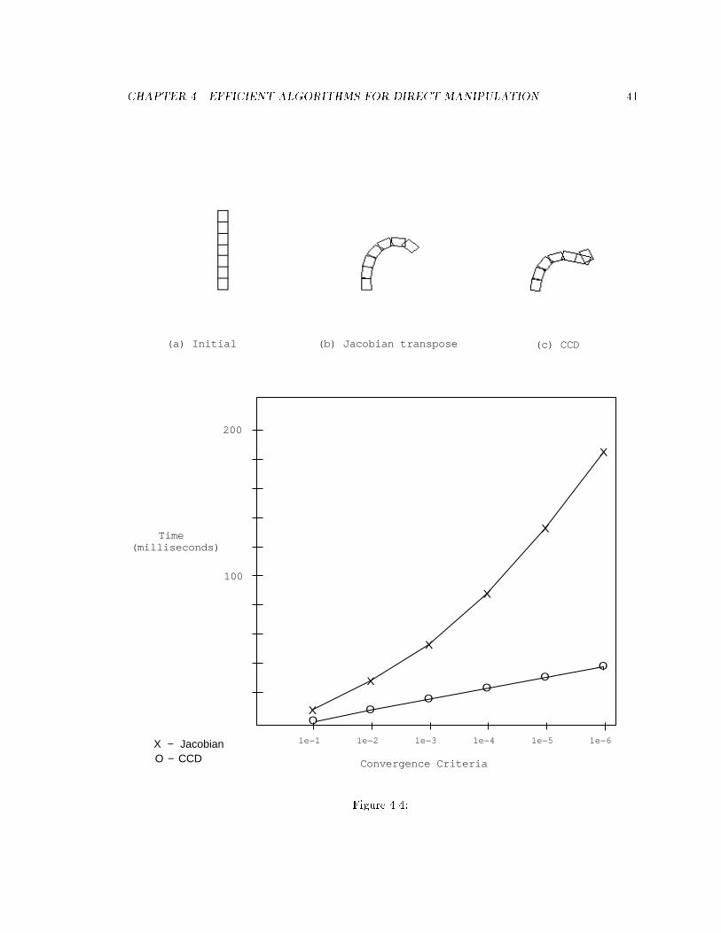
CHAPTER �� EFFICIENT ALGORITHMS FOR DIRECT MANIPULATION �

Convergence Criteria

1e−1 1e−2 1e−3 1e−4 1e−5 1e−6X − JacobianO − CCD

(a) Initial (b) Jacobian transpose (c) CCD

200

100

Time(milliseconds)

OO

OO

OO

X

X

X

X

X

X

Figure ��

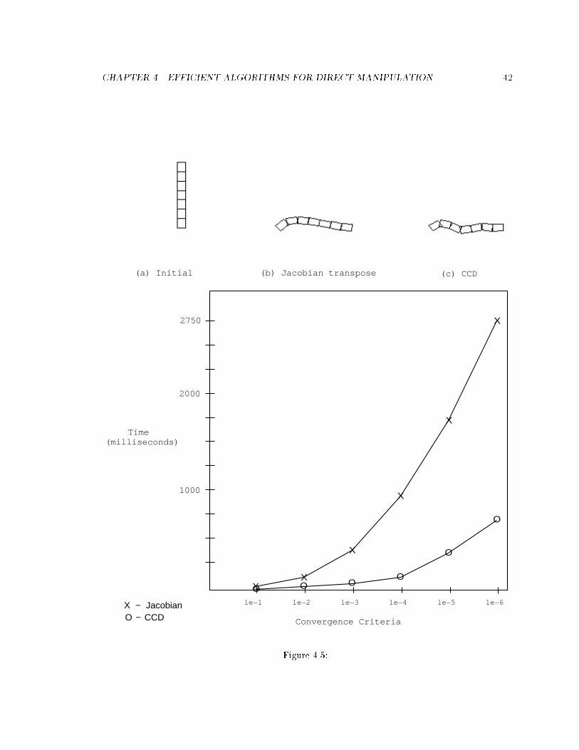
CHAPTER �� EFFICIENT ALGORITHMS FOR DIRECT MANIPULATION

Convergence Criteria

1e−1 1e−2 1e−3 1e−4 1e−5 1e−6X − JacobianO − CCD

(a) Initial (b) Jacobian transpose (c) CCD

2750

1000

Time(milliseconds)

O O OO

O

O

XX

X

X

X

X

2000

Figure ���

Chapter �

Incorporating Constraints

Inverse kinematic manipulation is a useful shortcut� but does not in itself provide any more function�

ality than simple forward kinematics� Creating a pose for a skeleton can be less tedious� but there

are still problems in trying to edit the pose without moving previously positioned body parts� It

would be useful� for example� to be able to specify that parts of the body should not move� no matter

how we manipulate the skeleton� Badler�s recent work �CP��� has shown the usefulness of being able

to impose constraints on a �gure during editing� The constrained optimization method employed

with Jack permits any constraint which can be expressed as a function of the skeleton state to be

speci�ed� However� with the exception of the experimental balance constraint described by Phillips

�PB���� this capability has not been exploited� The basic set of constraints available within Jack are

almost all simple geometric constraints on positions and orientations of body parts� It would seem

that even this limited set of constraints is enough to greatly improve interaction with a �gure�

In this chapter we consider how each of the manipulation techniques described in the previous

chapter can be used to satisfy multiple simple geometric constraints on the positions and orientations

of end�e�ectors within a skeleton� and discuss some of the performance and implementation issues

that arise�

��� Constraint Satisfaction

A manipulator� or a skeleton� can be considered a system described by a set of state variables � for

our purposes� joint rotations� Solving the inverse kinematic problem is essentially one of solving a

non�linear system of equations for these state variables� and there are a number of approaches one

can take to incorporate constraints in the solution process� We have already seen that constrained

optimization is one possibility� but there are other possibilities for the manipulation methods of the

previous chapter�

�

CHAPTER �� INCORPORATING CONSTRAINTS

The simplest approach is to use some variant of the penalty method� This method can be used

with any iterative technique� and the essential idea is that when a constraint is violated a restoring

force is introduced to push the system back into a legal state in which all constraints are satis�ed�

A feedback control loop monitors the state of the system and applies the appropriate penalty forces

as it detects constraint violations� An advantage of this approach is that if the constraints are not

initially met� the restoring forces pull the system towards a legal state� A disadvantage is that the

constraints cannot be enforced exactly� since the restoring force only comes into play after a constraint

has already been violated� Thus two points constrained to be coincident will appear to pull apart

slightly before the constraining force can pull them back together� For methods based on physical

simulation� the restoring forces are usually spring�based� If the springs are made su�ciently sti��

then the constraint violations may be small enough to be unnoticeable� But this causes problems

when trying to simulate the system� requiring tiny integration steps to retain numerical stability

�PFTV����

Both the Jacobian transpose method and the CCD method could be used within a control loop

to provide this sort of constraint satisfaction� In fact� due to the heuristic nature of the CCD method

and its reliance on strictly geometric information� this is the only option open� Before describing

a penalty�method approach based on the CCD method� we consider �rst a more comprehensive

solution which is a generalization of the Jacobian transpose method�

��� Maintaining Constraints

The approach taken is to consider the problem of maintaining a set of constraints which are already

satis�ed� rather than trying to satisfy constraints that have been violated� By assuming that the

system is already in a legal state� the problem is reduced to one of ensuring that changes to the system

never violate the constraints� The technique is based on well�known methods for implementing

constrained dynamics within physical simulations �Sur�� AW���� using the same sort of simpli�ed

�rst�order equations of motion described in Section ���� and by Gleicher �GW���� The essential idea

is that geometric constraints on an object are treated as mechanical connections which introduce

constraining forces into the system being simulated� When an external force is applied to the system�

some components of the applied force may be counteracted by these constraining forces� so that the

net force acting on the system does not violate the constraints� The nub of the problem is to

determine what these constraining forces are� given a set of geometric constraints which must be

satis�ed�

Figure ��� illustrates the concept for the simplest possible system� a point� The system�s state q

is simply the point�s location in space� A single constraint is imposed on the system� stating that the

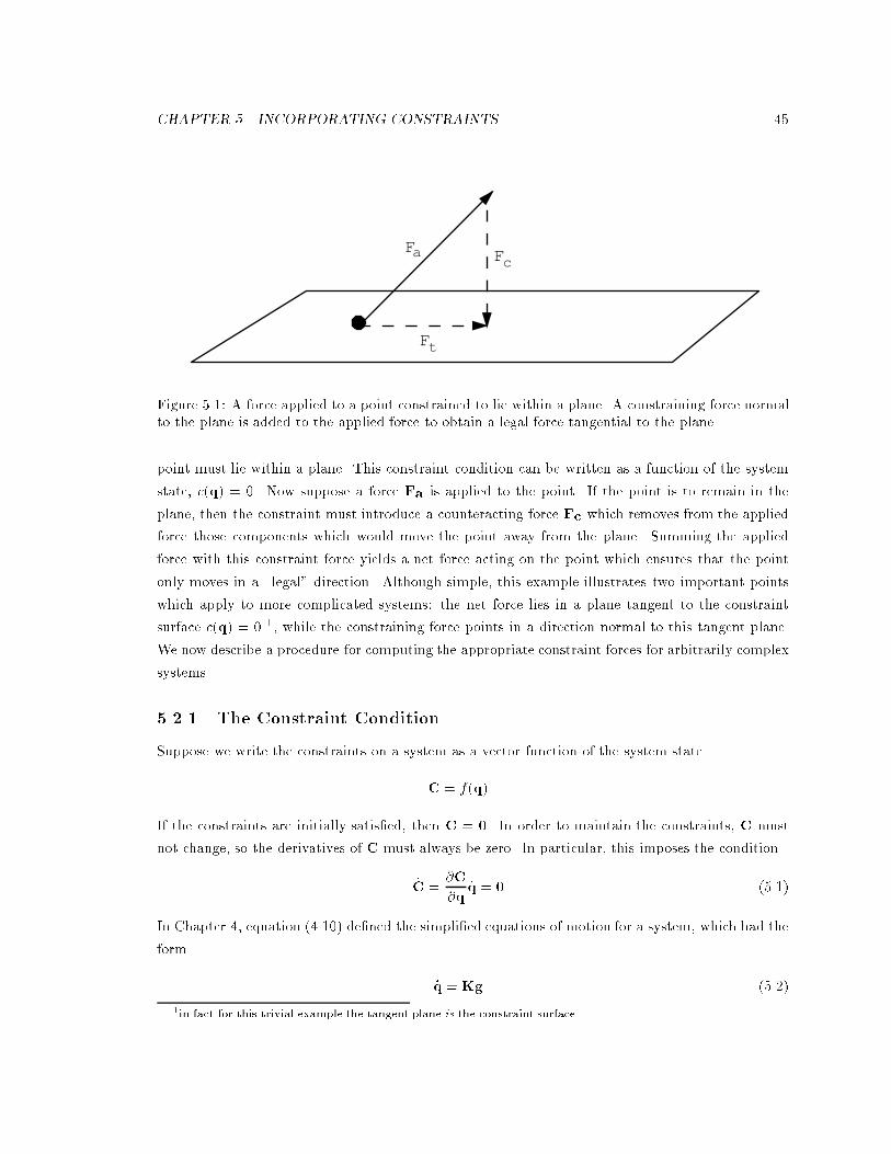
CHAPTER �� INCORPORATING CONSTRAINTS �

Fc

Ft

Fa

Figure ���� A force applied to a point constrained to lie within a plane� A constraining force normalto the plane is added to the applied force to obtain a legal force tangential to the plane�

point must lie within a plane� This constraint condition can be written as a function of the system

state� c�q� � �� Now suppose a force Fa is applied to the point� If the point is to remain in the

plane� then the constraint must introduce a counteracting force Fc which removes from the applied

force those components which would move the point away from the plane� Summing the applied

force with this constraint force yields a net force acting on the point which ensures that the point

only moves in a �legal� direction� Although simple� this example illustrates two important points

which apply to more complicated systems� the net force lies in a plane tangent to the constraint

surface c�q� � � �� while the constraining force points in a direction normal to this tangent plane�

We now describe a procedure for computing the appropriate constraint forces for arbitrarily complex

systems�

����� The Constraint Condition

Suppose we write the constraints on a system as a vector function of the system state

C � f�q�

If the constraints are initially satis�ed� then C � � In order to maintain the constraints� C must

not change� so the derivatives of C must always be zero� In particular� this imposes the condition

�C ��C

�q�q � �����

In Chapter � equation ����� de�ned the simpli�ed equations of motion for a system� which had the

form

�q � Kg ����

�in fact for this trivial example the tangent plane is the constraint surface

CHAPTER �� INCORPORATING CONSTRAINTS �

for some generalized force g acting on the system state� Substituting this equation into ������ and

denoting the constraint Jacobian matrix by Jc � �c�q � the constraint condition becomes

�C � JcKg � � �����

Any generalized force g acting on the system which satis�es this condition will not violate the

constraints�

����� Computing the Constraint Jacobian Matrix

The constraint Jacobian matrix Jc describes how the individual constraints change as the state

variables vary� The section above introduced the constraint vector C�q�� which is made up of m

scalar constraint functions c��q�� � � � � cm�q�� If there are n state variables q�� � � � � qn� then Jc is an

m� n matrix� Typically there are more state variables than there are constraints �

In practice� constraints are not speci�ed on q directly� but rather on more meaningful geometric

entities �such as points or orientations�� which are themselves functions of the state q� For example�

suppose we wish to impose a constraint that the tip of a limb on an articulated skeleton� denoted

P�q�� should remain �xed at some location R� An appropriate constraint condition for this example

would be

�R� P�q��� �

In this case the constraint vector C consists of � scalar constraints� one on each of the x� y� and z

components of P

C�q� � � c��Px�q��� c��Py�q��� c��Pz�q�� �

��Rx � Px�

�� �Ry � Py��� �Rz � Pz�

�

Each scalar constraint ci contributes a single row �ci�qj

to the constraint Jacobian matrix� Thus

each geometric constraint contributes a block of r rows to the matrix� where r is the dimension of

the geometric quantity �e�g� r � � for a point constraint�� Since geometric constraints are expressed

in terms of functions of q� the chain rule is applied to calculate the Jacobian entries� In the case

above� for example�

�ci�qj

��ci�Pk

�Pk

�qj

Typically a single constraint will depend on only a few of the system state variables� If the

left foot of the sample skeleton of Figure ��� is constrained to some location� for example� the arm

CHAPTER �� INCORPORATING CONSTRAINTS

joint variables have no e�ect on this constraint� Thus the i�th row of Jc� corresponding to the

constraint ci� usually contains just a few non�zero elements� It is important that this sparsity in

Jc be exploited and preserved� sparse matrix techniques o�er substantial performance gains over a

naive implementation�

����� Computing the Constraint Force

In Chapter it was shown that an external force applied to a point on an articulated skeleton could be

converted to a generalized force g on the skeleton state by the Jacobian transpose method� However�

the g of equation ����� is the net generalized force on the system� As such� it may include the sum

of multiple forces applied to various points on a skeleton� More to the point� it must also include

some �unknown� constraining forces which prevent the applied forces from violating the constraints

imposed on the system� In general� the net force is considered to be a sum of known applied forces

and of unknown constraint forces� g � ga� gc� Substituting this into the constraint condition �����

yields the linear system of equations

JcKgc � �JcKga ����

in which only the constraining generalized force vector gc is unknown�

Equation ���� simply states that an appropriate constraining force is one which� when added

to the applied forces� causes the constraint derivatives to be zero� But this is too ambiguous� since

the system is usually under�constrained and there may be many constraining forces gc which satisfy

equation ����� One approach to removing this ambiguity is to insist that the constraint force must

lie in a direction in which the system may not move � �just as the constraining force of Figure ���

does�� Recalling the discussion in Chapter � about the Singular Value Decomposition �SVD�� this

implies that the constraint force must lie within the range of the constraint Jacobian matrix Jc�

Thus for constrained systems in general� the constraint force gc is restricted to lie in the range of

Jc� while the net force g must lie in its null space� This is a generalization of the speci�c example

presented in Figure ����

If the constraint force is in the range of Jc� then gc � Jc for some vector � Therefore equation

���� can be written as

JcKJcT � �JcKga �����

and solved for the vector of Lagrange multipliers � Once the Lagrange multipliers are known� the

constraint force which removes the illegal components of the applied force is computed as

gc � Jc �����

�this restriction follows from the principle of virtual work Pau���

CHAPTER �� INCORPORATING CONSTRAINTS �

Note that computing gc requires the solution to a linear system of equations� even though the

constraints themselves may be non�linear�

����� Solving for Lagrange Multipliers

The linear system ����� must be solved to �nd the Lagrange multiplier vector

� � �� � � � � m �

Note that the number of equations in the system is equal to the dimension of the constraint vector

C� Any method for solving sets of linear equations can be applied here�

A method recommended here to solve the system emphasizes robustness over speed� Due to the

structure of most articulated skeletons� it is impossible to avoid ill�conditioning in ����� all of the

time �Mac���� To cope with this� the system is solved using the truncated SVD of the left�hand

m�m matrix JcKJcT � combined with a backsubstition algorithm �PFTV���� The truncated SVD

is formed from the original SVD by zeroing any �small� singular values� which e�ectively throws

away any ill�conditioned components of the matrix �PFTV��� MK���� This solution method does

not take advantage of any sparsity in the matrix� but has the advantage of being robust in cases

where ill�conditioning occurs�

����� Feedback

The discussion so far has been based on the assumption that the constraints are initially satis�ed�

and that they remain so� To handle cases in which the initial state violates some constraints� or

where numerical inaccuracies cause constraint violations� an additional feedback term is added to

the basic equation of motion ����

�q � K�ga � gc�� kCJcT ��� �

This term e�ectively adds a penalty spring to the system� the strength of which is proportional to

the magnitude of the constraint deviation C�

����� Overview

Equation ��� � is the complete simpli�ed equation of motion for a constrained system� Constraints

are maintained by evaluating the right hand side of the equation� using the methods outlined in the

sections above� to �nd the state variable velocities �q� A single integration step then yields a new state

q which respects any constraints imposed on the system� In an interactive setting� the procedure

iterates as the user applies changes to the system state through the user interface� Screen updates

occur after each iteration� to provide feedback� Figure �� provides an overview of the procedure

CHAPTER �� INCORPORATING CONSTRAINTS �

for a single iteration� Note that equation ��� � is a generalization of the Jacobian transpose method

of chapter � in the absence of any constraints on the system� the equation reduces to the simple

formula introduced earlier�

��� Implementation Issues

The basic constrained equation of motion ��� � has a regular structure which lends itself to an object�

oriented implementation� A solver for the equation only needs to know a few things� the length and

value of a global state vector q� how to evaluate a number of functions of q� and how to evaluate a

matrix of partial derivatives with respect to q for each of these functions�

Using software �objects� which respond to speci�c requests to provide these pieces of information�

a generic constraint solver can be written which is insulated from the speci�c details of articulated

skeletons� The solver queries these objects to obtain the information it needs to assemble a global

system of constrained equations of motion� solves the system� and then communicates the results

back to some of the �objects�� Implementing this method of maintaining constraints requires three

di�erent types of these �objects�� skeletons� handles and constraints�

����� Skeletons as Objects

Each skeleton is considered a single �object�� which contributes variables to the solver�s global state

vector q� Each skeleton must be able to respond to requests for speci�c pieces of information that

the solver requires� In addition� a method must be provided by which the solver can communicate a

solution back to the skeleton� If each skeleton provides these capabilities� the solver does not need

to know anything about the internal structure of the skeleton itself� The solver must be able to

� query a skeleton for the length of its state vector

� query a skeleton for its state variable vector

� query a skeleton for its scaling matrix K

� send a skeleton a new state vector re�ecting the solution

����� Handles on Skeletons

A handle is an abstraction representing a geometric quantity associated with a skeleton� whose value

depends on the skeleton�s internal state� A handle can refer to something as simple as the position

of a joint within the skeleton� or as complex as the location of the skeleton�s center of mass� Handles

are the geometric entities upon which constraints may later be imposed� and to which forces may be

applied�

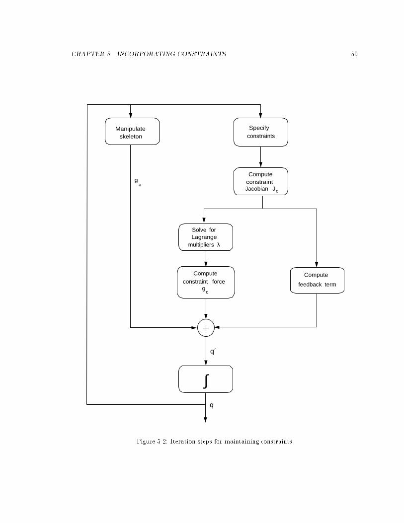
CHAPTER �� INCORPORATING CONSTRAINTS ��

Specifyconstraints

Computeconstraint force

gc

Solve forLagrange

multipliers λ

Compute

feedback term

∫

+

ComputeconstraintJacobian Jc

q

q´

skeleton

ga

Manipulate

Figure ��� Iteration steps for maintaining constraints

CHAPTER �� INCORPORATING CONSTRAINTS ��

Each handle attached to a skeleton knows how to compute a function of the skeleton�s state�

h�q skeleton�� A number of handle types can be de�ned� each computing a di�erent quantity� These

might include

� A point handle which computes the global position of some point de�ned within a local joint

coordinate system� �e�g� a point on the left shin� � inches below the knee�

� An orientation handle which computes the global orientation of a local joint coordinate system�

� A center�of�mass handle which computes the global position of a skeleton�s center of mass�

computed as a weighted average of each body part�s center of mass�

Usually a single handle will depend on only a subset of the joints within a skeleton� When queried

for its state vector� a skeleton should return only those elements of q skeleton which are referenced

by a handle� This will keep the total number of variables in the constrained system to a minimum�

In addition to the function h�q skeleton�� each handle must also know how to compute the Jacobian

matrix Jh�qskeleton� ��h

�qskeleton� The constraint solver will query each handle for this information

when assembling the global constraint Jacobian matrix Jc� Implementing a new handle type is

straightforward� requiring only � handle�speci�c routines to be coded� These routines are responsible

for initializing the handle� computing the handle function h� and computing the handle�s Jacobian

matrix Jh�

����� Constraints on Handles

Constraints can be applied to the quantities computed by a handle� The simplest constraints are

those that constrain a handle to a geometric constant� Useful examples of this include

� constraining a point handle to a given location

� constraining a point handle to a plane

� constraining a point handle to a line

� constraining an orientation handle to a given orientation

These simple constraints would be useful for specifying interactions with a static environment� For

example� the feet of a �gure can be constrained to lie in the plane de�ned by the �oor� or the hand

can be constrained to the rung of a ladder� To specify more complex behaviours� constraints could

also be created between two handles� For example� a �gure�s hands could be constrained to stay

clasped together by creating a point handle on each hand� then specifying an equality constraint

between these two handles�

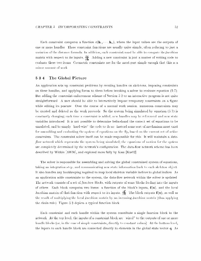
CHAPTER �� INCORPORATING CONSTRAINTS �

Each constraint computes a function c�h�� � � � �hn�� where the input values are the outputs of

one or more handles� These constraint functions are usually quite simple� often reducing to just a

variation of the distance formula� In addition� each constraint must be able to compute its Jacobian

matrix with respect to its inputs� �c�h

� Adding a new constraint is just a matter of writing code to

evaluate these two items� Geometric constraints are for the most part simple enough that this is a

minor amount of work�

����� The Global Picture

An application sets up constraint problems by creating handles on skeletons� imposing constraints

on these handles� and applying forces to them before invoking a solver to evaluate equation ��� ��

But adding the constraint enforcement scheme of Section �� to an interactive program is not quite

straightforward� A user should be able to interactively impose temporary constraints on a �gure

while editing its posture� Over the course of a normal work session� numerous constraints may

be created and deleted as the work proceeds� So the system being simulated by equation ��� � is

constantly changing� each time a constraint is added� new handles may be referenced and new state

variables introduced� It is not possible to determine beforehand the correct set of equations to be

simulated� and to simply �hard�wire� the code to do so� Instead some sort of mechanism must exist

for assembling and evaluating the system of equations on the �y� based on the current set of active

constraints� The constraint solver itself can be made responsible for this� It will maintain a data�

�ow network which represents the system being simulated� the equations of motion for the system

are completely determined by the network�s con�guration� The data��ow network scheme has been

described by Witkin �AW���� and explored more fully by Kass �Kas���

The solver is responsible for assembling and solving the global constrained system of equations�

taking an integration step� and communicating new state information back to each skeleton object�

It also handles any bookkeeping required to map local skeleton variable indices to global indices� As

an application adds constraints to the system� the data��ow network within the solver is updated�

The network consists of a set of function blocks� with outputs of some blocks feeding into the inputs

of others� Each block computes two items� a function of the block�s inputs� f �x�� and the local

Jacobian matrix of that function with respect to its inputs� �f�x � The block outputs f �x�� as well as

the result of multiplying the local Jacobian matrix by an incoming Jacobian matrix �thus applying

the chain rule�� Figure ��� depicts a typical function block�

Each constraint and each handle within the system contribute a single function block to the

network� At the top level� the inputs of a constraint block are �wired� to the outputs of one or more

handle blocks �or� in the case of simple constraints� directly to constant values�� At the bottom level�

the inputs to each handle block are connected directly to elements in the global state vector q� As

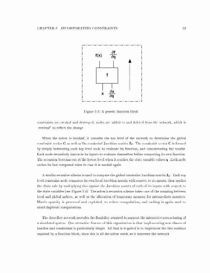
CHAPTER �� INCORPORATING CONSTRAINTS ��

f

f(x)

x ∂x∂q

∂f∂q

Figure ���� A generic function block�

constraints are created and destroyed� nodes are added to and deleted from the network� which is

�rewired� to re�ect the change�

When the solver is invoked� it consults the top level of the network to determine the global

constraint vector C as well as the constraint Jacobian matrix Jc� The constraint vector C is formed

by simply instructing each top level node to evaluate its function� and concatenating the results�

Each node recursively instructs its inputs to evaluate themselves before computing its own function�

The recursion bottoms out at the lowest level when it reaches the state variable values q� Each node

caches its last computed value in case it is needed again�

A similar recursive scheme is used to compute the global constraint Jacobian matrix Jc� Each top

level constraint node computes its own local Jacobian matrix with respect to its inputs� then applies

the chain rule by multiplying this against the Jacobian matrix of each of its inputs with respect to

the state variables �see Figure ����� The solver�s recursion scheme takes care of the mapping between

local and global indices� as well as the allocation of temporary memory for intermediate matrices�

Matrix sparsity is preserved and exploited� to reduce computation� and caching is again used to

avoid duplicate computations�

The data��ow network provides the �exibility required to support the interactive restructuring of

a simulated system� One attractive feature of this organization is that implementing new classes of

handles and constraints is particularly simple� All that is required is to implement the two routines

required by a function block� since this is all the solver needs as it traverses the network�

CHAPTER �� INCORPORATING CONSTRAINTS �

An Example

Consider the problem of constraining the tips of a �gure�s hands to its hips� This can be accomplished

by �rst creating four point handles on the �gure�

� handle h� on the tip of the right hand

� handle h� on the right hip

� handle h� on the tip of the left hand

� handle h� on the left hip

To �x the hands to the hips� two equality constraints on these handles are created

c� � �h� � h���

c� � �h� � h���

Figure �� shows the resulting data��ow network constructed by the constraint solver� Each handle

references a few variables within the skeleton�s state vector� these variables are concatenated to

form the global state vector q� The handle function blocks compute their respective point locations

and feed the results to the constraint function blocks� These compute the distances between the

incoming points� and the block function outputs are concatenated to form the ��element � global

constraint vector C� Each block also computes its own local Jacobian matrix with respect to its

inputs� multiplies it with an incoming matrix and passes the result along� The matrix outputs of

the constraint blocks contribute sparse rectangular blocks to the global constraint Jacobian Jc�

Any time an element of q changes value� a �disable cache� signal is triggered on any handle block

connected to the element� This signal percolates up through the network� forcing any block that is

encountered to discard its cached data� The next time the solver evaluates the network� only these

blocks will recompute their outputs� When the network has been re�evaluated� the solver has all the

information it needs to evaluate equation �� �

����� Summary

This constraint enforcement procedure has some attractive characteristics� Most importantly� con�

straints can theoretically be maintained exactly� since any forces acting on the system which would

cause a constraint violation are removed� The procedure is quite general� as well� constraints and

handles can be arbitrarily complex functions� and are therefore not restricted to referring to geomet�

ric quantities alone� The data��ow network architecture is extensible� since adding new handle and

constraint types is simply a matter of writing a handful of functions�

� for this example� two sets of x� y� and z scalar constraints�

CHAPTER �� INCORPORATING CONSTRAINTS ��

C Jc

1c2c

1h 2h 3h4h

q

Figure ��� Example network�

CHAPTER �� INCORPORATING CONSTRAINTS ��

The main drawback to the approach is that the solution cost is dominated by the O�n�� cost

of solving a linear system for the Lagrange multipliers� of which there is one for each of n scalar

constraints in the system being simulated� For even a few simple geometric constraints� the solution

time at this bottleneck quickly degrades to the point where interaction becomes di�cult� But Surles

�Sur�� has shown that when constraints are applied to articulated structures with speci�c charac�

teristics� the resulting system of equations can be solved in linear time� under certain conditions�

This result is promising� but is recent enough that it has not been pursued for this thesis�

A sample implementation of the method outlined above both con�rms its potential as well as the

limitations imposed by the bottleneck� Retaining interactive update rates for any reasonably complex

skeleton� with just a few position and orientation constraints applied� is di�cult given current CPU

performance� Simple Euler integration� not surprisingly� introduces numerical instabilities� due to

cumulative errors� when the integration stepsize is large enough to provide reasonable interactive

feedback� Adopting more robust adaptive integration methods is not necessarily helpful either�

These methods typically require multiple evaluations of equation ��� � per iteration� and since it

is so expensive to compute� the refresh rate drops dramatically and the interface tends to feel

unresponsive� In addition� adaptive stepsizing implies that some steps will be thrown away entirely

when the stepsize must be reduced in order to retain accuracy� As a result� one iteration may take

much longer to complete than another� so screen updates occur at irregular intervals and consequently

the interface is perceived as being �jerky� and unresponsive� However� these are problems which

will disappear as CPU performance improves to the point where accuracy in the solution can be

maintained at interactive update rates�

Another source of potential stability problems is the feedback term of equation ��� �� This term

su�ers from the usual problems associated with spring�based constraint enforcement� a high spring

constant k leads to a sti� set of equations which are unstable� while a low value for k permits

noticeable constraint violations� Choosing a good spring constant value can be di�cult� and is

currently done purely on a trial�and�error basis� Ideally the feedback spring should be a loose one

�i�e� k is �small��� with the assumption that as CPU performance improves it will be possible to

perform enough iterations between screen updates to eliminate any noticeable constraint violations�

Trying to eliminate the inevitable �drifting� of a system away from its constraints� a result of

numerical inaccuracies� by using a high spring constant is almost sure to introduce severe stability

problems�

Given current CPU speeds� this technique seems better suited to solving constraint problems

o��line than in an interactive setting� Our goal is to develop immediately useful interactive tools

for working with non�trivial skeletons� and this method cannot be considered practical yet for this

CHAPTER �� INCORPORATING CONSTRAINTS �

purpose on modestly powered workstations� Instead we will consider a penalty�force method based

on the CCD algorithm as a substitute with which we can experiment in an interactive editor�

��� A CCD�based Penalty Method

The previous method is capable of handling multiple constraints imposed on di�erent parts of a

skeleton� To accomplish the same with the CCD method requires some slight modi�cations to the

basic algorithm presented in Chapter � Whereas the basic algorithm considered just a serial chain

of links and a single goal� solving for multiple constraints means we must also consider branches in

the manipulator and more than one goal� as shown in Figure ����

The scheme of Chapter solved the problem for a serial chain by traversing from the end�e�ector

in towards the base� at each joint adjusting the joint parameter to minimize an error measure derived

from the current end�e�ector position and a known goal� In a branching chain with multiple end�

e�ectors and multiple goals� a joint may contribute to the position of more than one end�e�ector�

so potentially more than one goal must be considered when varying the joint variable� Also� the

algorithm depends on the inward traversal scheme� distal joints must be solved �rst before a more

proximal one can be considered� This precludes treating the multiple�goal problem as a series of

single�goal problems which can be solved sequentially�

A recursive traversal of the hierarchy from the leaves in towards the root ensures that all sub�

problems at a joint are solved before the joint itself is considered� Each joint instructs all of its

children to solve for any constraints that may be applied to end�e�ectors in their sub�tree� Then the

joint variable which minimizes the summed error measure from each child sub�tree can be computed�

The only change from the previous CCD algorithm is that the traversal must now consider branches

A

B

Figure ���� A branching chain with two end�e�ector constraints

CHAPTER �� INCORPORATING CONSTRAINTS ��

in a chain� and that the error measure equation ����� of Chapter becomes a summation

E�q� �nXi��

Epi�q� �Eoi�q� �����

over the n constraints which are distal to the current joint� The net e�ect of this change is that the

coe�cients k�� k�� and k� must be computed by summing equations �������� over each distal

end�e�ector goal� before a minimizing change in the current joint variable can be computed� The

procedure must iterate until either all end�e�ector constraints have been satis�ed� or until successive

iterations produce negligible changes� indicating that the constraints are con�icting and cannot be

simultaneously satis�ed�

This recursive scheme resembles Badler�s early heuristic approach �BMW� � for positioning a

�gure with multiple constraints� although the CCD method for computing a minimizing change in a

joint variable appears to di�er from the one used there�

This penalty method approach is arguably inferior to the more comprehensive scheme outlined

previously� Constraints are only approximately enforced� so we can expect to see some �drift� on

segments that are constrained to stay in place� Also� we are restricted to geometric constraints

due to the CCD method�s reliance on geometric relationships alone� Nevertheless the method is

usually stable enough to perform adequately at interactive update rates� and gives us a means of

experimenting with constraints within our interactive editor� In our prototype implementation�

instabilities do occur when position and orientation constraints con�ict with each other� but this can

be alleviated with appropriate weighting factors on the individual constraints�

Chapter �

An Interactive Editor

To place the discussion of the preceding chapters in context� an interactive program for animating

articulated �gures is introduced here� The program is designed to create keyframed motion sequences

for arbitrary skeletons� and has been both a motivation and a testbed for the ideas developed

in this thesis� Both the Jacobian transpose and the CCD methods have been implemented� and

the application interface modi�ed to accomodate direct inverse kinematic manipulation� as well as

constrained manipulation� This chapter brie�y describes the program and the manipulation interface�

�� A System Overview

The Sequence Editor is an interactive tool for creating and editing keyframed movement sequences

for a single arbitrary skeletal �gure� Its primary function has been to act as the �movement creation�

window of a motion planning package �CWGL��� for choreographers� whose needs are quite di�erent

from those of computer animators� To a typical user planning the movement of multiple �gures in a

work space� a rough approximation of a movement that can be created quickly can be more valuable

than a more realistic animation that would take hours to perfect� Consequently the program�s design

has favoured ease of use over functionality� The hope is that direct manipulation and constraint

satisfaction based on the methods of the previous chapters can improve the quality of movement

created with the editor while retaining a simple and intuitive user interface�

Before describing the interface itself� some of the terminology warrants a brief explanation�

����� Skeletons

The program itself knows nothing about skeletons speci�cally� a skeleton appears as an abstract data

type supported by a toolkit library of routines� The toolkit supports the creation� manipulation and

��

CHAPTER �� AN INTERACTIVE EDITOR ��

animation of skeletons de�ned by a simple ASCII �le format� Figure ��� � shows a sample description

for a simple approximation to a human �gure� Any valid skeleton description can be read in to the

editor and animated�

As the example shows� each skeleton is simply a collection of named joints arranged in a hierarchy�

The joints are either rotary or prismatic� each with a single degree of freedom� Compound joints with

multiple degrees of freedom �e�g� ball�and�socket� can be modelled as a series of these single DOF

joints sharing the same location� Associated with each joint are a number of attributes� including

the joint type �rotary or prismatic�� the local axis �axes� of freedom� and local limits on the range

of movement of the joint� Polygonal objects may be attached to any joint node in the hierarchy�

These �rigid� objects comprise the appearance of the skeleton and are drawn as they are encountered

during a display traversal of the hierarchy�

A skeleton maintains an internal state vector q� consisting of all the joint variable values as well

as a translation vector for the skeleton as a whole� This information is enough to completely de�ne

the location and shape of the skeleton for a single frame� An application can animate a skeleton by

repeatedly loading the skeleton state q and instructing the skeleton to display itself�

The toolkit now supports inverse kinematic control over a skeleton by allowing the application

to identify both a base and an end�e�ector within the joint hierarchy� A desired position and�or

orientation for the end�e�ector may then be speci�ed� and the skeleton instructed to solve the

inverse kinematic problem using either of the methods of the previous chapter� The internal state q

is automatically updated to re�ect the solution to the problem� This isolates the application from

the details of the inverse kinematic algorithms�

����� The Sequence

A sequence is an abstract data type for storing skeleton animation data� it represents the movements

of a skeleton over some period of time� An application may query a sequence to determine the

skeleton state at any frame of the animation� Although a sequence could encapsulate a procedural

motion model� for this discussion a sequence will be de�ned as a series of keyframed poses� each of

which speci�es the state vector q at a particular frame� When a sequence is queried for the skeleton

state at a frame between key frames� an interpolated state is computed on�the��y and returned� For

each rotating joint� either linear or splined quaternion � interpolation �Sho��� may be performed�

For each translating joint� either linear interpolation or generalized Catmull�Romspline interpolation

�KB�� may be used� Currently� no further control over the interpolation process is provided� other

�courtesy of Phil Peterson�a quaternion is a compact representation for rotations� with some appealing properties

CHAPTER �� AN INTERACTIVE EDITOR ��

head

right hand

right arm

left hand

left armtorso

pelvis

right leg left leg

right foot left foot

define joint "right leg" object "r_lleg.pol" offset 0 −0.32 0 hinge x 0 170 mass 1 orientation 0 0 0 mirror "left leg"end joint

# Example .scr file for a stick figure.

define skeleton "stickman" joint "pelvis" group "Upper body" joint "torso" group "Right Arm" joint "right arm" joint "right hand" end group group "Left arm" joint "left arm" joint "left hand" end group joint "head" # "head" is a child of "torso" end group group "Right leg" joint "right leg" joint "right foot" end group group "Left leg" joint "left leg" joint "left foot" end group end skeleton

Figure ���� Sample skeleton description

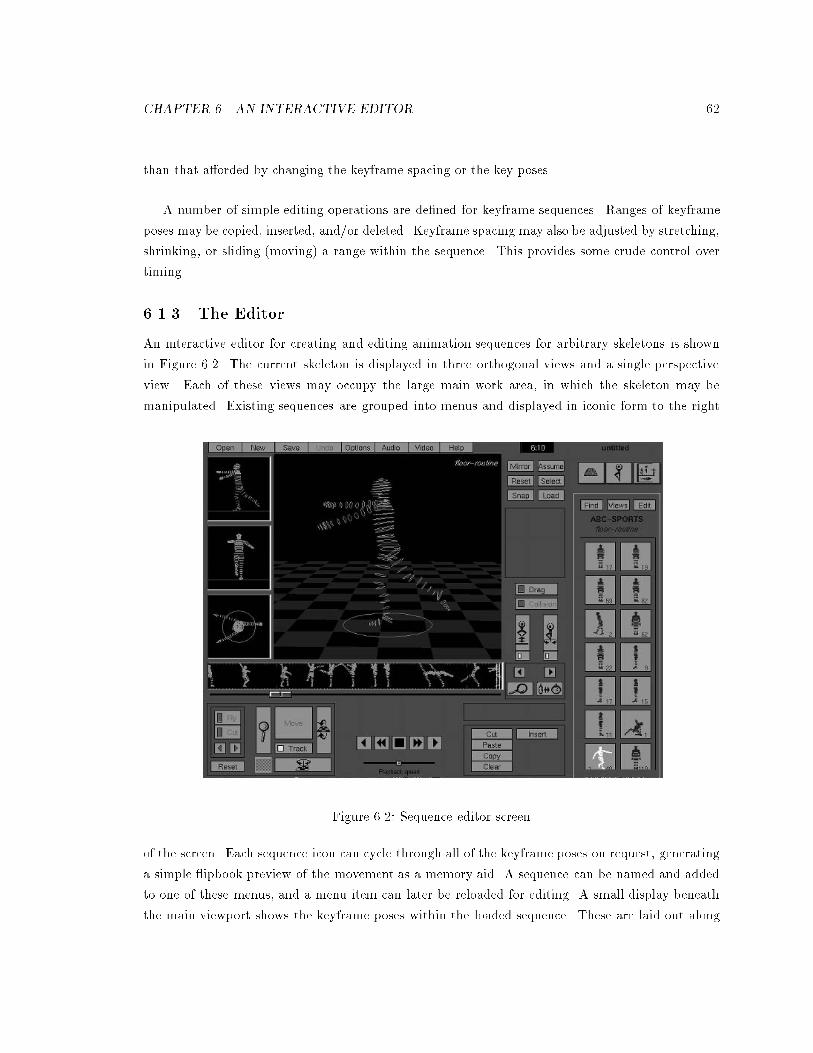
CHAPTER �� AN INTERACTIVE EDITOR �

than that a�orded by changing the keyframe spacing or the key poses�

A number of simple editing operations are de�ned for keyframe sequences� Ranges of keyframe

poses may be copied� inserted� and�or deleted� Keyframe spacing may also be adjusted by stretching�

shrinking� or sliding �moving� a range within the sequence� This provides some crude control over

timing�

����� The Editor

An interactive editor for creating and editing animation sequences for arbitrary skeletons is shown

in Figure ��� The current skeleton is displayed in three orthogonal views and a single perspective

view� Each of these views may occupy the large main work area� in which the skeleton may be

manipulated� Existing sequences are grouped into menus and displayed in iconic form to the right

Figure ��� Sequence editor screen

of the screen� Each sequence icon can cycle through all of the keyframe poses on request� generating

a simple �ipbook preview of the movement as a memory aid� A sequence can be named and added

to one of these menus� and a menu item can later be reloaded for editing� A small display beneath

the main viewport shows the keyframe poses within the loaded sequence� These are laid out along

CHAPTER �� AN INTERACTIVE EDITOR ��

a timeline to indicate the keyframe spacing� A set of VCR�like transport controls are provided for

playing back the animated sequence in the main display area�

The small timeline provides a convenient interface for copying� cutting and pasting ranges of

keyframes within a sequence� as well as modifying the keyframe spacing� But the key poses them�

selves must be created or modi�ed by adjusting the skeleton displayed in the main window� For

manipulating the skeleton� forward kinematic controls are provided in the form of sliders for adjust�

ing individual joints within the skeleton one at a time� In addition� the interface has been modi�ed

to permit inverse kinematic manipulation of the skeleton� In this mode the user may use the methods

presented in the previous chapter to update multiple joints by dragging one body part around� The

implementation of this interface for direct manipulation is brie�y described below�

�� Direct Manipulation

With direct manipulation� the user adjusts the skeleton by selecting and dragging a body part� rather

than adjusting individual joints� A dragging session begins when a body part is selected with the

mouse� and ends when the mouse button is released� Dragging is a positioning mechanism only� it

does not directly control the orientation of the selected part� To support dragging� the interface

must provide a way of identifying a serial chain of joints within the skeleton which will be considered

a manipulator� as well as a way of unambiguously specifying end�e�ector goals for the chain�

Identifying the Chain

A chain of joints within the skeleton is de�ned when a body part is �rst selected� at which time

both a base joint and an end�e�ector must be determined� To determine a base joint� the skeleton

hierarchy is traversed backwards from the selected part towards the root� Three separate interaction

modes control how far up the tree this traversal proceeds before stopping at a joint which becomes

the base of the chain� The stopping criteria corresponding to each of the three dragging modes are

�� stop when the parent joint has a body part attached to it

� stop when the parent joint has multiple children

�� stop when a named joint is reached

The �rst of these results in only the selected body part being dragged� and is the direct manipulation

equivalent of positioning the part using the forward kinematic slider controls� The second results in

a chain which extends from the nearest branch in the hierarchy� and is therefore a useful default to

use when dragging limbs� Selecting and dragging a hand� for example� would move the entire arm

without disturbing the torso� The third interaction mode permits the user to override these default

CHAPTER �� AN INTERACTIVE EDITOR �

behaviours by explicitly naming a joint from which the chain extends� Thus the user can specify a

torso joint as the chain base� for example� in which case pulling on the arm would result in a bend

of the spine�

In addition to the base of the chain� the end�e�ector position must be known� since that is the

point being dragged� There are two possible approaches to determing the end�e�ector location when

a user points at a body segment and presses the mouse button� The �rst is to explicitly compute the

point on the body segment underneath the cursor� by casting a ray and intersecting it with the object�

The alternative is to pre�de�ne locations within the skeleton which may be selected for dragging� the

locations of the joints themselves� for example� This requires either that the locations be displayed

in some iconic form so the user can select one� or that the cursor �warp� to the nearest one when the

mouse button is pressed� The initial decision was to choose the former method� explicitly computing

a point on the surface of the object and making that point the location of the end�e�ector frame�

This gave mixed results� On one hand it allowed the user to click anywhere on the object for

dragging without any disconcerting cursor �warping�� On the other hand� having the end�e�ector

frame located on the object surface often resulted in unexpected twisting of the segment� especially

with the Jacobian method� As a compromise� the current implementation places the end�e�ector

halfway along the segments axis of self�rotation� �warping� the cursor to the corresponding onscreen

location� Locating the end�e�ector along the segment axis eliminates the problem of unexpected

twisting�

Determining an End�E�ector Goal

To compute new goal positions for the end�e�ector as the cursor moves around on the screen� we

must resolve the ambiguity in mapping a D screen location to a �D location� The solution adopted

here is to cast a ray through the cursor into the world� and to �nd the point on this line which

is closest to the end�e�ector� This point becomes the goal position for the current iteration� This

technique provides reasonable behaviour in both orthographic and perspective views�

With an orthographic projection� the cast ray is parallel to the line of sight� and the closest point

on the line will lie in the plane perpendicular to the ray and containing the end�e�ector� In this case

the end�e�ector is constrained to lie within the plane while it is dragged around� In a perspective

projection view� the cast ray may diverge from the line of sight� and the shortest path from the

end�e�ector to the ray is no longer constrained to lie parallel to the image plane� The end�e�ector

is therefore free to move in any direction� and may even be �pushed� and �pulled� towards and

away from the viewer with a little practice� Figure ��� illustrates the case for both perspective and

orthographic projections�

CHAPTER �� AN INTERACTIVE EDITOR ��

goal

goal

(a) (b)

Figure ���� Plan view of goal determination in �a� an orthographic view� and �b� a perspective view

Once the new goal position for the end�e�ector has been computed� the skeleton is instructed

to solve the inverse kinematic problem� the user can select the solution method to use by setting

a program option� The screen is refreshed and the cursor location resampled after each iteration�

to provide responsive feedback� Of course� when a single iteration is insu�cient to solve the most

recent problem� the movement of the skeleton lags behind the cursor� In practice this small tracking

delay has not been a problem�

To provide some control over the responsive behaviour of the skeleton� the user can interactively

modify weighting parameters at each individual joint� This is particularly useful when the CCD

method is used� allowing a the responsiveness of a chain to be varied from that of a sti� rod to that

of a set of loosely coupled links�

�� Constraints

As an additional positioning aid� a small set of constraints have been de�ned which the user may

apply to any segment of a skeleton� The most useful of these are intended to lock limb extremities

in place while the pose is being edited� Currently constraints are enforced by iteratively solving a

set of persistent inverse kinematic goals using the CCD method� This restricts us to a set of simple

geometric goals�

� Locking an end�e�ector position

� Locking an end�e�ector orientation� This can be a partial lock of only one or two directions

�e�g� lock Y orientation only��

CHAPTER �� AN INTERACTIVE EDITOR ��

� A weighted combination of both of these

� Constraining an end�e�ector to lie within a plane

To apply a lock the user selects a segment� then makes a lock selection from a menu� Once created�

a lock remains in place until it is explicitly deleted� A lock can be edited� to change either its type� its

importance weighting� or the joints which can contribute to maintaining the lock� The lock location

or orientation can also be modi�ed by either dragging the lock� or twisting the end�e�ector through

a set of sliders�

The intent is that locks represent constraints which are to be maintained during any subsequent

positioning of the �gure� To achieve this� after each editing operation of a �gure� whether through

direct manipulation or the forward kinematic slider controls� a number of iterations of the multiple�

goal CCD solver are performed prior to each screen refresh� When the number of iterations performed

is insu�cient to satisfy any constraints violated by the editing operation� some drifting from the lock

constraint positions is unavoidable� But a button is provided for invoking the solver explicitly until

all constraints are met to the user�s satisfaction� The user may also change the number of iterations

performed between screen refreshes� On a high�performance machine this number can be set high to

minimize visible constraint violations� on a low�performance machine a smaller number can improve

the responsiveness of the interface� at the cost of constraint violations becoming more noticeable�

Locking constraints are particularly useful when applied to the supporting limbs of a �gure� In

the example of Figure �� the �gure�s feet are constrained to stay in place by locking both their

position and orientation� The �rst image shows the position at which the locks are created� In the

second image the pelvis has been tilted to lean the �gure� and in the third image a twist has been

applied to the pelvis� In all three images the foot positions and orientations are maintained� and the

CCD solver is fast enough that the pelvis can be tilted and twisted interactively without noticeable

sliding of the feet� For this example� � iterations between screen refreshes were su�cient to maintain

the constraints with negligible drift� and provide an update rate of �� frames per second on a Silicon

Graphics R���� Entry Level Indigo workstation� This update rate is inadequate for animation� but

quite su�cient for interactive positioning�

While locking end�e�ectors in position is useful for creating a series of consistent keyframe poses�

there still remains the problem of maintaining the constraints at the interpolated in�between frames�

There is no guarantee that an end�e�ector locked to some position in two adjacent keyframes will

remain in that position if joint angles are merely interpolated between the poses� Figure ��� illustrates

the problem� The �rst and last images are keyframes in which the feet have been constrained to

the same position and orientation� The image in the middle is the result of interpolating joint

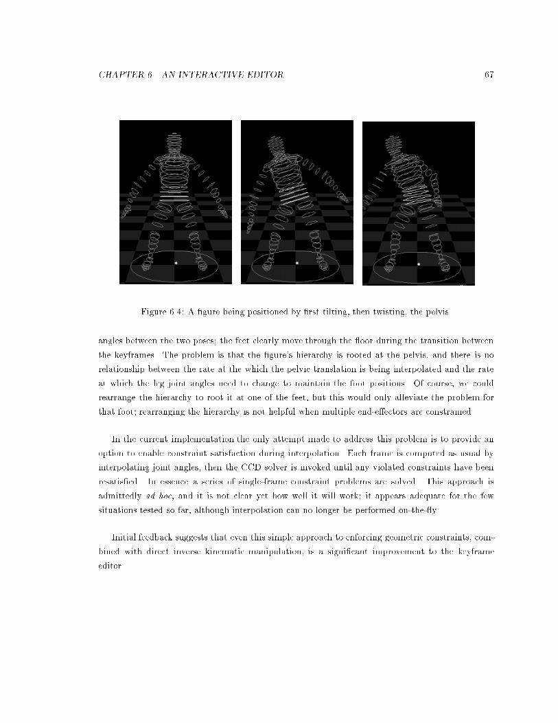
CHAPTER �� AN INTERACTIVE EDITOR �

Figure ��� A �gure being positioned by �rst tilting� then twisting� the pelvis�

angles between the two poses� the feet clearly move through the �oor during the transition between

the keyframes� The problem is that the �gure�s hierarchy is rooted at the pelvis� and there is no

relationship between the rate at the which the pelvic translation is being interpolated and the rate

at which the leg joint angles need to change to maintain the foot positions� Of course� we could

rearrange the hierarchy to root it at one of the feet� but this would only alleviate the problem for

that foot� rearranging the hierarchy is not helpful when multiple end�e�ectors are constrained�

In the current implementation the only attempt made to address this problem is to provide an

option to enable constraint satisfaction during interpolation� Each frame is computed as usual by

interpolating joint angles� then the CCD solver is invoked until any violated constraints have been

resatis�ed� In essence a series of single�frame constraint problems are solved� This approach is

admittedly ad hoc� and it is not clear yet how well it will work� it appears adequate for the few

situations tested so far� although interpolation can no longer be performed on�the��y�

Initial feedback suggests that even this simple approach to enforcing geometric constraints� com�

bined with direct inverse kinematic manipulation� is a signi�cant improvement to the keyframe

editor�

CHAPTER �� AN INTERACTIVE EDITOR ��

Figure ���� �a� First keyframe pose �b� Interpolated pose �c� Second keyframe pose

Chapter �

Conclusion

�� Summary

We have examined solutions to the inverse kinematic problem applied to manipulating articulated

skeletons in an interactive keyframe animation editor� As alternatives to previously published algo�

rithms in the graphics literature� a pair of simple algorithms have been described which can provide

relatively inexpensive direct manipulation of a �gure� The �rst of these is really just an application

of a simple minimization method� but its application to inverse kinematics has not previously been

made explicit� The second is a new heuristic algorithm adopted and modi�ed from the robotics liter�

ature� The advantages and disadvantages of each have been discussed and their relative performances

gauged�

Methods by which each algorithm can be used to satisfy constraints during manipulation have

been developed� and their respective advantages and disadvantages discussed� An implementation

of the simpler approach has been incorporated into a keyframe editor� and the interface brie�y

described�

As a byproduct� a toolkit library for de�ning and manipulating skeletons has been implemented

which insulates an application from the details of creating� editing� drawing and animating a �gure�

A skeleton is also able to solve inverse kinematic problems posed by the application� allowing the

application to deal with interface issues rather than dealing explicitly with inverse kinematic algo�

rithms� This also allows new inverse kinematic solution methods to be implemented and added to

the toolkit without requiring modi�cations to the application�

��

CHAPTER �� CONCLUSION �

�� Results

After experimenting with several inverse kinematic methods in the course of this work� some things

have become apparant� The �rst is that inverse kinematic algorithms all exhibit problems of one

type or another� no one approach seems uniformly superior to others� The methods presented here

should not necessarily be considered any better than other approaches� but rather provide alternative

approaches which may be suitable in some applications�

The second point is that inverse kinematics as a positioning tool is a useful complement to� but

not a replacement for� simple forward kinematic positioning� In particular� for direct manipulation

inverse kinematics is really only useful for chains with relatively few degrees of freedom � single

limbs� for example� In fact� an interesting observation is that even with the ability to drag multiple�

jointed chains around many users of the editor described in Chapter � seem quite content with

the default dragging mode� which drags just a single body part� Informal feedback from users

suggests that while direct manipulation is a huge improvement to the interface over the previous

slider�based positioning� the value of multiple�joint positioning is not quite so clear� In fact� trying

to position a chain with many degrees of freedom with direct manipulation is often likely to cause

unwanted changes to the skeleton� For example� trying to bend the spine of a �gure by pulling on its

�ngers is probably asking too much � in the absence of additional constraints specifying how changes

should be distributed among the joints� any method is likely to give unnatural results� Joint limits

provide some constraints� as do the weighting parameters at each joint� but these do not seem to

be adequate� particularly for manipulating recognizable bodies� Inverse kinematic methods which

perform quite acceptably for disembodied chains or mechanical robots do not necessarily translate

well to �animate� �gures� the results can often appear unnatural� This problem is that the term

�unnatural� is subjective� and di�cult to quantify� More powerful positioning tools are likely to

result from considering these factors more carefully�

Either of the inverse kinematic algorithms presented in Chapter is adequate for interactive direct

manipulation� They are both simple to implement� and are fast enough to provide good feedback

for gross positioning tasks� However if high accuracy is a requirement and interactive response time

not so much of a concern� then other solution methods may o�er better performance�

���� Comments about Constraints

In Chapter �� the choice of the CCD�based penalty method for implementation within the �gure

animation editor was largely based on performance issues� the alternative Lagrange multiplier�based

approach was deemed too demanding for interactive use on a typical workstation� This problem

is temporary� however� and it is worth reconsidering the decision in light of continuing increases in

CHAPTER �� CONCLUSION �

CPU power� At the same time we can speculate a little about what types of constraints might be

useful to develop and how constraints might be used for animation as well as manipulation�

Given su�cient CPU speed to retain numerical stability� the Lagrange multiplier approach is the

more general of the two� The CCD�based method is fast because it reduces a di�cult problem to a

series of simpler ones which can be solved analytically using only simple geometric quantities� But

for problems more complicated than solving position and orientation constraints the reduction to

analytical form is not always possible� so the approach is limited to these types of constraints� In

contrast the Lagrange multiplier method could be used to enforce many di�erent types of constraints�

including non�geometric ones� the only requirement is that the constraints be some function of the

joint variables within a �gure�

Looking Ahead

What sorts of constraints� other than the obvious geometric ones� might be useful for �gure ma�

nipulation Initial experimentation with the constraint solver implemented in the animation editor

indicates that geometric constraints alone� while useful� are not always enough� Too often a solution

which is correct in the sense that all geometric constraints are satis�ed� seems incorrect because it

puts the �gure into an awkward looking pose� Think� for example� of a person going from a standing

position into a crouch� The natural tendency is for the knees to move apart as the person crouches�

because that is the comfortable way to crouch� To manipulate a standing �gure in the editor into a

crouch� one might lock the toes of each foot in place and then pull the pelvis down to make the �gure

crouch� But without any other information about how the legs should move� one is just as likely to

see the knees move together as the �gure crouches� as to see them move together� Perhaps this could

be recti�ed by specifying additional geometric constraints on the knees� but choosing and specifying

these auxiliary constraints would probably be di�cult and time�consuming� A useful alternative

would be a standard set of constraints which applied to the �gure at all times� These might include

constraints to avoid uncomfortable postures� or postures which would place a person o��balance�

The latter can be implemented as a constraint on a �gure�s center�of�mass� a computable quantity

given a set of joint angles� while the former would require some function which measured comfort�

or �naturalness�� given the same set of variables�

In addition to manipulation� constraints could also be useful in animating a �gure� A natural

place to start would be to consider animating the constraint values� Animating a position constraint�

for example� might de�ne a trajectory for some limb extremity to follow� A simultaneous animated

orientation constraint would control the orientation of the extremity as it traversed the trajectory�

But for complex motions� constraints will probably be more helpful in describing a desired movement

with some sort of scripting approach� For example� the movements of the support foot of a walking

CHAPTER �� CONCLUSION

biped might be described in terms similar to the following

�After heel strike� the heel of the foot maintains its position until the ball of the foot

touches the ground� For a short period the entire foot remains locked in place while the

body moves forward� Toward the end of the step� the heel of the foot breaks contact with

the ground �rst� followed shortly after by the ball of the foot��

A description such as this identi�es a number of simple constraints which are in e�ect during the

movement� If the description were more speci�c about the time intervals and locations involved we

would have a fairly detailed script for animating the stance foot during a walk� A simple scripting

language could be implemented which would allow movements such as this to be described textu�

ally� A script would need to specify a set of constraints to be imposed� and provide some way of

activating and deactivating these constraints over the course of a movement� An interpreter for such

a descriptive scripting language would be a useful tool for �gure animation�

�� Directions

There are plenty of problems still to be addressed� At a low level of detail it is worth determining

whether the performance of the Lagrange multiplier constraint satis�er can be improved upon� First�

Surles has shown that some constraint problems for articulated �gures can be solved in linear time

�Sur��� He lists a number of prerequisites for this� but in the context of chemical protein modelling�

which is his application area� An analysis of these prerequisites and what they mean in the context

of articulated skeleton manipulation would be useful� A second area which could be explored to

speed up the solution process is to consider Maciejewski�s incremental algorithm for computing the

SVD �MK���� the referenced papers on this topic are interesting reading� and may suggest alternate

approaches to the inverse kinematic problem in general�

Designing interactive interfaces which make e�ective use of constraints is challenging� and deserves

some attention� How should constraints be represented Selected Edited What should happen

when constraints con�ict with each other How should constraints be animated and controlled over

time What about constraints involving multiple �gures

And �nally� do inverse kinematics and constraints provide a convenient layer upon which higher

level procedural motion models can be built An interesting exercise would be to extend Bruderlin�s

walking algorithm to handling uneven terrain� making use of the basic techniques described in this

thesis to achieve and maintain footholds�

Bibliography

�AG��� W� Armstrong and M� Green� The dynamics of articulated rigid bodies for purposes of

animation� The Visual Computer� ����!�� �����

�AN��� L� Alt and A� Nicolas� Animating articulated structures with multiple goals� In Proceed�

ings of Computer Graphics� pages ��!�� �����

�AW��� W� Welch A� Witkin� M� Gleicher� Interactive dynamics� Computer Graphics� ���

March �����

�Bai��� J� Bailleiul� Avoiding obstacles and resolving kinematic redundancy� In Proc� �� Int�

Conf� on Robotics and Automation� April �����

�BB� � R� Barzel and A� Barr� Modeling with dynamic constraints� In SIGGRAPH Course

Notes� Topics in Physically�Based Modelling� ��� �

�BC��� A� Bruderlin and T� Calvert� Goal�directed dynamic animation of human walking� Com�

puter Graphics� �������!� July �����

�BH��� R� Bartels and I� Hardtke� Speed adjustment for keyframe interpolation� In Proceedings

of Graphics Interface� pages �!��� �����

�BMW� � N� Badler� K� Manoochehri� and G� Walters� Articulated �gure positioning by multiple

constraints� IEEE Computer Graphics and Applications� �����!��� June ��� �

�BN��� L� Brotman and A� Netravali� Motion interpolation by optimal control� Computer Graph�

ics� ������!���� August �����

�CHP��� J� Chadwick� D� Haumann� and R� Parent� Layered construction for deformable animated

characters� Computer Graphics� ������!�� July �����

�Coh�� M�F� Cohen� Interactive spacetime control for animation� Computer Graphics� ����

July ����

�

BIBLIOGRAPHY

�CP��� N� Badler C� Phillips� J� Zhao� Interactive real�time articulated �gure manipulation

using multiple kinematic constraints� In Proceedings� ��� Symposium on Interactive �D

Graphics� pages �!��� �����

�CWGL��� T�W� Calvert� C� Welman� S� Gaudet� and C� Lee� Composition of multiple �gure

sequences for dance and animation� In Proceedings of CG International� �����

�DSS��� H� Das� J�J� Slotine� and T�B� Sheridan� Inverse kinematic algorithms for redundant

systems� In Proceedings IEEE Int�l� Conference on Robotics and Automation� pages

�!�� �����

�FW��� D� Forsey and J� Wilhelms� Techniques for interactive manipulation of articulated bodies

using dynamic analysis� In Proceedings of Graphics Interface� pages �!��� �����

�Gir��� M� Girard� Interactive design of �d computer�animated legged animal motion� In Pro�

ceedings� Workshop on Interactive �D Graphics� pages ���!���� �����

�Gir��� M� Girard� Constrained optimization of articulated animal movement in computer ani�

mation� In N� Badler� B� Barsky� and D� Zeltzer� editors� Making Them Move� Mechan�

ics� Control� and Animation of Articulated Figures� chapter ��� pages ��!�� Morgan

Kaufmann Publishers�Inc�� San Mateo� Ca�� �����

�GM��� M� Girard and A� Maciejewski� Computational modeling for the computer animation of

legged �gures� Computers Graphics� ��������! �� July �����

�GMW��� P� Gill� W� Murray� and M� Wright� Practical Optimization� Academic Press� New York�

NY� �����

�Gom��� J� Gomez� Twixt� A �d animation system� Computers and Graphics� �������!���

March �����

�GP��� B� Guenter and R� Parent� Computing the arc length of parametric curves� IEEE

Computer Graphics and Applications� ������ ! �� May �����

�Gre��� T�N�E� Greville� The pseudoinverse of a rectangular or singular matrix and its application

to the solution of systems of linear equations� SIAM Review� �������!�� January �����

�GW��� M� Gleicher and A� Witkin� Di�erential manipulation� In Proceedings of Graphics Inter�

face ���� �����

�Hah��� J�K� Hahn� Realistic animation of rigid bodies� Computer Graphics� �����!����

August �����

BIBLIOGRAPHY �

�HS��� P� Hanrahan and D� Sturman� Interactive animation of parametric models� The Visual

Computer� ����!��� �����

�IC� � P� Isaacs and M� Cohen� Controlling dynamic simulation with kinematic constraints�

behaviour functions and inverse dynamics� Computer Graphics� ������!� July

��� �

�IC��� P� Isaacs and M� Cohen� Mixed methods for complex kinematic constraints in dynamic

�gure animation� The Visual Computer� ���!���� �����

�Kas�� M� Kass� Condor� Constraint�based data�ow� Computer Graphics� ���� July ����

�KB�� J� Korein and N� Badler� Techniques for goal�directed motion� IEEE Computer Graphics

and Applications� ���� �!��� ����

�KB�� D� Kochanek and R� Bartels� Interpolating splines with local tension� continuity� and

bias control� Computer Graphics� ��������!�� July ����

�KH��� C�A� Klein and C�H� Huang� Review of pseudoinverse control for use with kinemati�

cally redundant manipulators� IEEE Transactions on Systems� Man� and Cybernetics�

�������!��� March�April �����

�Las� � J� Lasseter� Principals of traditional animation applied to �d computer animation� Com�

puter Graphics� ������!� July ��� �

�LWZB��� P� Lee� S� Wei� J� Zhao� and N� Badler� Strength guided motion� Computer Graphics�

�����!�� �����

�Mac��� A� A� Maciejewski� Dealing with the ill�conditioned equations of motion for articulated

�gures� IEEE Computer Graphics and Applications� ��������!� May �����

�MK��� A�A� Maciejewski and C�A� Klein� The singular value decomposition� Computation and

applications to robotics� International Journal of Robotics Research� ����� December

�����

�NN��� Z�R� Novakovic and B� Nemec� A solution of the inverse kinematics problem using the

sliding mode� IEEE Transactions on Robotics and Automation� ���� !�� April �����

�Pau��� R�P� Paul� Robot Manipulators� Mathematics� Programming� and Control� MIT Press�

Cambridge� MA� �����

�PB��� C� Phillips and N� Badler� Interactive behaviours for bipedal articulated �gures� Com�

puter Graphics� �������!��� July �����

BIBLIOGRAPHY �

�PFTV��� W�H� Press� B�P� Flannery� S�A� Teukolsky� and W�T� Vetterling� Numerical Recipes

in C � The Art of Scienti�c Computing� Cambridge University Press� Cambridge� MA�

�����

�SB��� S� Steketee and N� Badler� Parametric keyframe interpolation incorporating kinetic

adjustment and phrasing control� Computer Graphics� ��������!�� July �����

�Sho��� K� Shoemake� Animating rotation with quaternion curves� Computer Graphics�

�������!�� July �����

�SS� � L� Sciavicco and B� Siciliano� A dynamic solution to the inverse kinematic problem of

redundant manipulators� In IEEE Int�l Conference on Robotics and Automation� pages

����!����� March ��� �

�Ste��� G� Stern� Bbop � a program for ��dimensional animation� In Nicograph Proceedings�

pages ��!�� �����

�Stu� � D� Sturman� Interactive keyframe animation of �d articulated models� In SIGGRAPH

Course Notes� Computer Animation� �D Motion Speci�cation and Control� pages � !��

��� �

�Sur�� M�C� Surles� An algorithm with linear complexity for interactive� physically�based mod�

eling of large proteins� Computer Graphics� ���� July ����

�SZ��� K� Sims and D� Zeltzer� A �gure editor and gait controller for task level animation� In

SIGGRAPH Course Notes� Synthetic Actors� The Impact of Arti�cial Intelligence and

Robotics on Animation� �����

�WC��� L�C�T� Wang and C�C� Chen� A combined optimization method for solving the inverse

kinematics problem of mechanical manipulators� IEEE Transactions on Robotics and

Automation� �����!��� August �����

�WCH��� B� Wyvill�M� Chmilar� and C� Herr� A simplemodel of human animation� In SIGGRAPH

Course Notes� Synthetic Actors� The Impact of Arti�cial Intelligence and Robotics on

Animation� �����

�WE�� W�A� Wolovich and H� Elliot� A computational technique for inverse kinematics� In

Proceedings of ��rd Conference on Decision and Control� pages ����!���� December

����

�Wil��� J� Wilhelms� Virya � a motion control editor for kinematic and dynamic animation� In

Proceedings of Graphics Interface� pages ��!��� �����

BIBLIOGRAPHY

�Wil� � J� Wilhelms� Using dynamic analysis for realistic animation of articulated bodies� IEEE

Computer Graphics and Applications� �����! � June ��� �

�Wil��� J� Wilhelms� Dynamic experiences� In N� Badler� B� Barsky� and D� Zeltzer� editors� Mak�

ing Them Move� Mechanics� Control� and Animation of Articulated Figures� chapter ���

pages ��!��� Morgan Kaufmann Publishers�Inc�� San Mateo� Ca�� �����

�WK��� A� Witkin and M� Kass� Spacetime constraints� Computer Graphics� ������!����

August �����

�ZB��� J� Zhao and N� Badler� Real time inverse kinematics with joint limits and spatial con�

straints� Technical Report Technical Report MS�CIS������� University of Pennsylvania�

�����

�Zel�a� D� Zeltzer� Motor control techniques for �gure animation� IEEE Computer Graphics

and Applications� ������!��� ����

�Zel�b� D� Zeltzer� Representation of complex animated �gures� In Proceedings of Graphics

Interface� pages ��!��� ����