inverse optimization: a new perspective on the black ...dbertsim/papers/finance/inverse optimization...

OPERATIONS RESEARCHVol. 60, No. 6, November–December 2012, pp. 1389–1403ISSN 0030-364X (print) � ISSN 1526-5463 (online) http://dx.doi.org/10.1287/opre.1120.1115

© 2012 INFORMS

Inverse Optimization: A New Perspective on theBlack-Litterman Model

Dimitris BertsimasSloan School of Management, Massachusetts Institute of Technology, Cambridge, Massachusetts 02139,

[email protected]

Vishal GuptaOperations Research Center, Massachusetts Institute of Technology, Cambridge, Massachusetts 02139,

[email protected]

Ioannis Ch. PaschalidisDepartment of Electrical and Computer Engineering, Boston University, Boston, Massachusetts 02215,

[email protected]

The Black-Litterman (BL) model is a widely used asset allocation model in the financial industry. In this paper, we providea new perspective. The key insight is to replace the statistical framework in the original approach with ideas from inverseoptimization. This insight allows us to significantly expand the scope and applicability of the BL model. We provide aricher formulation that, unlike the original model, is flexible enough to incorporate investor information on volatility andmarket dynamics. Equally importantly, our approach allows us to move beyond the traditional mean-variance paradigm ofthe original model and construct “BL”-type estimators for more general notions of risk such as coherent risk measures.Computationally, we introduce and study two new “BL”-type estimators and their corresponding portfolios: a mean varianceinverse optimization (MV-IO) portfolio and a robust mean variance inverse optimization (RMV-IO) portfolio. These twoapproaches are motivated by ideas from arbitrage pricing theory and volatility uncertainty. Using numerical simulationand historical backtesting, we show that both methods often demonstrate a better risk-reward trade-off than their BLcounterparts and are more robust to incorrect investor views.

Subject classifications : finance: portfolio optimization; programming: inverse optimization; statistics: estimation.Area of review : Financial Engineering.History : Received May 2011; revisions received November 2011, January 2012; accepted June 2012. Published online in

Articles in Advance November 20, 2012.

1. IntroductionThe Black-Litterman (BL) model is a widely used assetallocation model in the financial industry. Introduced inBlack and Litterman (1992), the model uses an equilibriumanalysis to estimate the returns of uncertain investmentsand employs a Bayesian methodology to “blend” theseequilibrium estimates with an investor’s private informa-tion, or views, about the investments. Computational expe-rience has shown that the portfolios constructed by thismethod are more stable and better diversified than thoseconstructed from the conventional mean-variance approach.Consequently, the model has found much favor with practi-tioners. The U.S. investment bank Goldman Sachs regularlypublishes recommendations for investor allocations basedon the BL model and has issued reports describing thefirm’s experience using the model (Bevan and Winkelmann1998). A host of other firms (Zephyr Analytics, BlackRock,Neuberger Berman, etc.) also use the BL model at the coreof many of their investment analytics.

The model, however, does have its shortcomings. First, itis somewhat limited in the way it allows investors to specifyprivate information. Namely, it only allows investors tospecify views on asset returns, but not on their volatility

or market dynamics. Secondly, and more restrictively, themodel is predicated upon the mean-variance approach toportfolio allocation. A host of theoretical and empiricalwork suggests variance may not be a suitable proxy forrisk. As a consequence, other risk measures such as valueat risk (VaR) or conditional value at risk (CVaR) have beenexplored. (See, for example, Artzner et al. 1999, Bertsimaset al. 2004, Grootveld and Hallerbach 1999, Harlow 1991,Jorion 1997, Rockafellar and Uryasev 2002.)

Subsequent research has tried to address these short-comings. We mention only a few examples and refer thereader to Walters (2010) and the references therein for amore complete survey. Giacometti et al. (2007), Martelliniand Ziemann (2007), and Meucci (2005) extend beyondthe mean-variance paradigm, using “fat-tailed” distributionsto model asset returns, coupled with VaR or CVaR, andviews on the tail behavior of returns. By contrast, Pástor(2000) and Pástor and Stambaugh (2000) build upon theBayesian interpretation of the original model, using a gen-eral pricing model as their “prior.” Finally, Meucci (2008)and Meucci et al. (2011) formulate a further generalizationwithin the statistical framework, modeling “risk factors” (inlieu of asset returns) by a general distribution and solving

1389

INFORMS

holds

copyrightto

this

article

and

distrib

uted

this

copy

asa

courtesy

tothe

author(s).

Add

ition

alinform

ation,

includ

ingrig

htsan

dpe

rmission

policies,

isav

ailableat

http://journa

ls.in

form

s.org/.

Bertsimas, Gupta, and Paschalidis: Inverse Optimization: Black-Litterman Model1390 Operations Research 60(6), pp. 1389–1403, © 2012 INFORMS

a minimum entropy optimization to update this distribu-tion to one that incorporates a very general set of views. Inmost cases, this optimization is solved numerically, and inthe case when the distribution is constrained to belong to aparametric family, the optimization is usually nonconvex.

In this paper, we provide a new optimization-driven per-spective on the BL model that avoids many of the statis-tical assumptions of previous approaches. The key insightis to characterize the BL estimator as the solution to aparticular convex optimization problem. More specifically,we formulate a problem in inverse optimization—a setupwhere one is given an optimal solution to an optimizationproblem and seeks to characterize the cost function and/orother problem data. Initial research on inverse optimizationfocused on specific combinatorial optimization problems(see Heuberger 2004 for a survey). Later, Ahuja and Orlin(2001) provided a unified approach for linear programmingproblems using duality. Iyengar and Kang (2005) extendedthese ideas to conic optimization with an application tomanaging portfolio rebalancing costs.

Previous research, starting with Black and Litterman(1992), has drawn some connections between the BL modeland what many authors call “reverse optimization.” The keyidea, formalized in He and Litterman (1999), is to solvethe first-order optimality condition of a Lagrangean relax-ation of the Markowitz problem to derive the equilibriumreturns. It may not be clear how to generalize this approachto other constrained asset allocation problems. Often, asin Herold (2005), which considers a budget constraint andDa Silva et al. (2009), which considers information-ratioportfolio optimization, the authors are forced to rely on adhoc arguments. Furthermore, “reverse optimization” onlyprovides the equilibrium estimates. Most authors still use astatistical approach to blend in the views.

To the best of our knowledge, our work is the first tooffer a rigorous inverse optimization interpretation of theBL model. This has several advantages. First, it allowsus to completely characterize the set of “input data” inthe Markowitz problem in equilibrium and to incorporatemore general views, e.g., on volatility. Second, it enablesus to move beyond mean-variance and adopt more gen-eral risk metrics by leveraging robust optimization ideas.Further, our approach does not rely on specific distribu-tional assumptions on market returns; we construct theequilibrium estimates and blend them with views usingoptimization techniques. As such, our approach unifies sev-eral threads in the literature (Herold 2005, Krishnan andMains 2005, Martellini and Ziemann 2007). It can also bepotentially combined with the ideas in Meucci (2008) andMeucci et al. (2011) of modelling risk factors instead ofasset returns.

We summarize the major contributions of our paper asfollows:

1. By linking the BL model with inverse optimization,we provide a novel formulation that constructs equilibrium-based estimators of the mean returns and the covariancematrix.

2. Our framework permits greater freedom in the typeof private information and investor views expressible inthe model. Specifically, our formulation allows investors toincorporate views on volatility and market dynamics. Weleverage this freedom to create a new asset allocation pro-cedure we call the “mean-variance inverse optimization”(MV-IO) approach, which uses BL-type estimators in a set-ting motivated by the arbitrage pricing theory.

3. By drawing on ideas from robust optimization, wegeneralize the traditional Markowitz portfolio problem toone that can encompass risk metrics such as VaR, CVaR,and generic coherent risk measures.

4. We then use inverse optimization to construct BL-type estimators in this new model. We illustrate the powerof this method with what we call the robust mean varianceinverse optimization (RMV-IO) approach, which accommo-dates volatility uncertainty.

5. We provide computational evidence to show that MV-IO and RMV-IO portfolios often provide better risk-rewardprofiles and are more robust to incorrect or extreme viewsthan their BL counterparts.

The remainder of the paper is organized as follows:Section 2 briefly reviews the BL model. Section 3 derivesthe BL model from principles in inverse optimization andshows how it can be extended to include volatility estima-tion and views on volatility. Section 4 introduces a moregeneral portfolio allocation problem and constructs a BL-type estimator in this setting. Section 5 provides numericalresults illustrating the strengths and drawbacks of these newestimators compared to the original estimator. Finally, §6concludes and discusses some avenues for future research.

Throughout this paper we will use bold-faced capital let-ters 4è1P1 0 0 05 to indicate matrices, bold-faced lowercaseletters to indicate vectors 4x1 r1 0 0 05 and ordinary letters4L1 t1 0 0 05 to indicate scalars. The vector e refers to the vec-tor of all ones, 0 is the vector of all zeroes, and I is anidentity matrix. Finally, for a matrix A, we write A� 0 toindicate that A is positive semidefinite and A � 0 to indi-cate that A is positive definite.

2. The Black-Litterman ModelThis section reviews the original BL model to keep thepaper self-contained. For a complete treatment, see Blackand Litterman (1992) or He and Litterman (1999).

Consider a market with n risky assets and one risk-less asset where investors seek to maximize their expectedreturn subject to a threshold level of risk. We initially definerisk to be measured by the standard deviation of returns. In§4, we will generalize the notion of risk considerably. Inother words, investors solve the Markowitz portfolio allo-cation problem

(Markowitz) maxx

{

Ì′x+ 41 − e′x5rf 2√

x′èx¶ L}

1 (1)

where r ∈�n is the random vector of the risky asset returns,Ì ≡ Ɛ6r7 is the vector of mean asset returns, rf ∈ �+ is

INFORMS

holds

copyrightto

this

article

and

distrib

uted

this

copy

asa

courtesy

tothe

author(s).

Add

ition

alinform

ation,

includ

ingrig

htsan

dpe

rmission

policies,

isav

ailableat

http://journa

ls.in

form

s.org/.

Bertsimas, Gupta, and Paschalidis: Inverse Optimization: Black-Litterman ModelOperations Research 60(6), pp. 1389–1403, © 2012 INFORMS 1391

the return on the riskless asset, è ∈�n×n is the covariancematrix of asset returns, x ∈ �n is the fraction of wealthinvested in each risky asset, and L is an investor-specificthreshold level of risk. We assume that an investor can bor-row or invest at the riskfree rate.

The primary difficulty in solving (1) is finding a stableestimation procedure for Ì and è. The BL model suggestssuch a procedure. At a high level, the procedure blends twosources of information:

• Market Equilibrium: If all investors solve (1) for someinvestor-specific L, then there exists a value � ∈ �+ suchthat the expected returns Ì satisfy

Ì= rf e+ 2�èxmkt0 (2)

Here, xmkt is the percentage market capitalization of eachasset. By multiplying (2) by xmkt, observe that � =

4Ì− rf e5′xmkt/42xmkt′èxmkt50 In this sense, � measures the

risk-reward trade-off for the market portfolio. Finally, thereis some aggregate, but unobservable, value of L such thatxmkt is a solution to (1) and

�=

√

4Ì− rf e5′è−14Ì− rf e5/

42L50

These conditions collectively form the capital asset pricingmodel equilibrium (CAPM). (See Sharpe 1964 for classicalproofs of these results. Alternatively, we will derive theseequations as a special case of Theorem 2 in §4.)

• Private Information: Any particular investor may haveprivate information, or views, that are not shared by otherinvestors. The model expresses these views through sev-eral different portfolios p11p21 0 0 0 1pm for which the investorhas some estimate of the corresponding mean returnsq11 q21 0 0 0 1 qm. More compactly,

PÌ= q1 (3)

where P′ = 6p11p21 0 0 0 1pm7 and q′ = 4q11 q21 0 0 0 1 qm5.Assuming that both of these sources of information areat least approximately true, the BL procedure posits thefollowing statistical model:

r ≡ rf e+ 2�èxmkt0 (4)

Here Ì = r + År 1Pr = q+ Åv, � and è are estimates of �and è, respectively, and 4År 1Åv5 is a random noise vector.Although è may be estimated from historical data, � is,itself, not directly observable. Even though there are vari-ous proposals in the literature, to the best of our knowledgethere is no consensus on how to fit �. Observe that thechoice of � only affects the estimate of r and the resultingportfolio by a constant of proportionality.

By assuming that 4År 1Åv5 is distributed as a multivari-ate normal distribution, i.e., 4År 1Åv5 ∼ N401ì5 for somecovariance matrix ì, and that several other key quanti-ties are Gaussian and mutually independent, Black and

Litterman (1992) estimates 4Ì1è5 by the Bayesian update1

4ÌBL1èBL5 where

ÌBL=è−1

2

(

IP

)′

ì−1

(

rq

)

1 (5)

è2 =

[(

IP

)′

ì−1

(

IP

)]

1 èBL=è1 +è20 (6)

The quantities ì and è1 are unobservable and requireexogenous specification. A common approximation used inHe and Litterman (1999) is

è1 = è1 ì=

(

�0è 0

0 diag4�11 0 0 0 1 �m5

)

1 (7)

where �i ∈�+1 i = 01 0 0 0 1m represent the investor’s relativeconfidence in each view.

As pointed out in He and Litterman (1999), the originalpaper Black and Litterman (1992) does not mention Equa-tion (6) for èBL. Indeed, many references refer to Equa-tion (5) alone as the BL model. However, Equation (6)and the subsequent approximations are critically neededto solve the allocation Problem (1). As we will see, ourapproach avoids such approximations by directly estimat-ing the covariance matrix è.

Despite the number of statistical assumptions and exoge-nously specified parameters, this procedure yields stableestimates with good practical performance. We illustratethis procedure with an example that we will continue todevelop in the sequel.

2.1. An Example: Applying the BL Procedure

In the U.S. equity market, every stock is given a GlobalIndustrial Classification Standard (GICS) sector classifica-tion describing the industry to which the underlying com-pany belongs. The list of 10 possible classifications can befound in Table 1 with their average historic returns overthe previous 24 months, denoted Ìhist, and market share,denoted xmkt, as of May 1, 1998.2 We also present the his-torical covariance between the sectors in Table EC.1 ofthe electronic companion which is available as part of theonline version at http://dx.doi.org/10.1287/opre.1120.1115.We will use the BL procedure to construct a portfolio ofthese sectors.

First, consider using the given historical return andcovariance information directly in the Markowitz formula-tion (1). The resulting portfolio, denoted xhist, is displayedin Table 1. (All portfolios have been scaled to sum to 100for ease of comparison.) It has large long positions in someassets, large short positions in others, and almost no invest-ment in others—an allocation that does not match our intu-ition of a “well-diversified” portfolio. This phenomenon iscommon and highlights one of the difficulties in using theMarkowitz formulation (1) in practice.

INFORMS

holds

copyrightto

this

article

and

distrib

uted

this

copy

asa

courtesy

tothe

author(s).

Add

ition

alinform

ation,

includ

ingrig

htsan

dpe

rmission

policies,

isav

ailableat

http://journa

ls.in

form

s.org/.


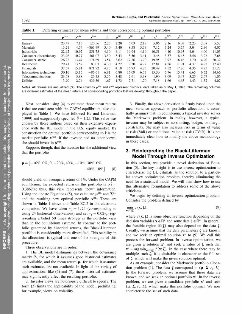
Table 1. Differing estimates for mean returns and their corresponding optimal portfolios.

Ìhist xmkt xhist r ÌBL xBL Ì1 x1 ÌMV xMV Ì2 ÌRob xRob

Energy 23047 7015 120056 2025 2020 5003 2019 5006 2016 6003 2023 2008 5057Materials 13021 4054 −863099 3040 3040 8058 3039 7012 3024 5075 3004 2096 4007Industrials 22092 10092 251073 4010 4011 10094 4010 10051 4010 10093 4004 4000 11003Consumer discretionary 23096 10077 361007 3050 3043 5056 3041 3048 3037 8045 3056 3028 7068Consumer staple 26022 13047 −171069 3054 3062 17036 3070 19095 3097 16016 3070 4020 20032Healthcare 29041 13057 83003 4030 4022 9020 4027 12081 4026 11091 4037 4023 12040Financials 37067 15081 871092 4013 4018 16093 4025 20049 4052 17026 4035 4073 21027Information technology 30016 15016 −86061 6081 6080 16009 6077 15030 6076 15041 6065 6052 14066Telecommunications 23058 5088 −26045 3056 3048 2061 3038 −1090 3009 3047 3025 2067 −1006Utilities 13090 2074 −439056 1067 1073 7071 1070 7018 1066 4063 1043 1052 4007

Notes. All returns are annualized (%). The columns Ìhist and xmkt represent historical data taken as of May 1, 1998. The remaining columnsare different estimates of the mean return and corresponding portfolios that we develop throughout the paper.

Next, consider using (4) to estimate those mean returnsr that are consistent with the CAPM equilibrium, also dis-played in Table 1. We have followed He and Litterman(1999) and exogenously specified �= 1025. This value waschosen by those authors based on their extensive experi-ence with the BL model in the U.S. equity market. Byconstruction the optimal portfolio corresponding to r is themarket portfolio xmkt. If the investor had no other views,she should invest in xmkt.

Suppose, though, that the investor has the additional viewthat the portfolio

p=[

−10%10%101−20%140%1−10%130%10%1

− 40%110%]

(8)

should yield, on average, a return of 1%. Under the CAPMequilibrium, the expected return on this portfolio is p′r =

003862%; thus, this view represents “new” information.Using the update Equations (5), we calculate ÌBL and èBL

and the resulting new optimal portfolio xBL. These areshown in Table 1 above and Table EC.2 in the electroniccompanion. We have taken �0 = 1/24 (corresponding tousing 24 historical observations) and set �1 = 0002�0, rep-resenting a belief 50 times stronger in the portfolio viewthan in the equilibrium estimate. In contrast to the port-folio generated by historical returns, the Black-Littermanportfolio is considerably more diversified. This stability inthe allocations is typical and one of the strengths of thisprocedure.

Three observations are in order:1. The BL model distinguishes between the covariance

matrix è, for which it assumes good historical estimatesare available, and the mean return Ì, for which it assumessuch estimates are not available. In light of the variety ofapproximations like (6) and (7), these historical estimatesmay significantly affect the resulting portfolio.

2. Investor views are notoriously difficult to specify. Theform (3) limits the applicability of the model, prohibiting,for example, views on volatility.

3. Finally, the above derivation is firmly based upon themean-variance approach to portfolio allocation; it essen-tially assumes that, in equilibrium, a typical investor solvesthe Markowitz problem. In reality, however, a typicalinvestor may be subject to no-shorting, budget, or marginconstraints. She may also measure risk in terms of valueat risk (VaR) or conditional value at risk (CVaR). It is notimmediately clear how to modify the above methodologyin these cases.

3. Reinterpreting the Black-LittermanModel Through Inverse Optimization

In this section, we provide a novel derivation of Equa-tion (5). The key insight is to use inverse optimization tocharacterize the BL estimate as the solution to a particu-lar convex optimization problem, thereby eliminating theneed for a statistical model. We will then show how to usethis alternative formulation to address some of the abovecriticisms.

We begin by defining an inverse optimization problem.Consider the problem defined by

minx∈X4Æ5

f 4x3Æ51 (9)

where f 4x3Æ5 is some objective function depending on thedecision variables x ∈�n and some data Æ ∈�m. In general,the feasible region X4Æ5 may also depend on the data Æ.Usually, we assume that the data parameters Æ are known,and we seek an optimal solution x∗ to (9). We call thisprocess the forward problem. In inverse optimization, weare given a solution x∗ and seek a value of Æ such thatx∗ = arg minx∈X4Æ5 f 4x3Æ50 In the case where there may bemultiple such Æ, it is desirable to characterize the full setof Æ, which will make the given solution optimal.

As an example, consider the Markowitz portfolio alloca-tion problem (1). The data Æ correspond to 4Ì1è1 rf 1L5.In the forward problem, we assume that these data areknown, and we seek an optimal portfolio x∗. In the inverseproblem, we are given a candidate portfolio x∗ and seek4Ì1è1 rf 1L5, which make this portfolio optimal. We nowcharacterize the set of such data.

INFORMS

holds

copyrightto

this

article

and

distrib

uted

this

copy

asa

courtesy

tothe

author(s).

Add

ition

alinform

ation,

includ

ingrig

htsan

dpe

rmission

policies,

isav

ailableat

http://journa

ls.in

form

s.org/.


Proposition 1. Consider the Markowitz problem (1), andassume we are given a candidate portfolio x∗. In addition,suppose that it is known a priori that è � 0 and L > 0.Then, 4Ì1è1 rf 1L5 solve the inverse problem for (1) if andonly if there exists a � such that:

x∗′

èx∗ ¶ L21 �4L2 − x∗′

èx∗5= 01

Ì− rf e− 2�èx∗ = 01 �¾ 01 L > 01 è� 00(10)

Proof. For any fixed values of the data with è � 01L > 0, the forward problem is convex and satisfies a Slatercondition. Thus, it is necessary and sufficient that any opti-mal solution x satisfies the Karush-Kuhn-Tucker (KKT)conditions (Bertsekas 1999). The KKT conditions are pre-cisely the Equations (10), with x∗ replaced by x and theconstraints è � 0 and L > 0 omitted. (We have rewrittenthe constraint

√x′èx¶ L as x′èx¶ L2 for convenience.)

Now consider the inverse problem. We have alreadyestablished that it is both necessary and sufficient for x∗ tosatisfy the system (10) to be optimal. If we now interpret x∗

as given and view the remaining parameters as unknown,it follows that any solution to the inverse problem mustsatisfy this system of equations with x∗. �

Because è is a covariance matrix, the assumption è� 0is natural. On the other hand, it is possible that L= 0, butthis case is somewhat degenerate. Intuitively, it correspondsto a situation where an investor will tolerate no risk. Itis possible to show that the system (10) is still necessaryand sufficient in this case. We provide the details in thee-companion.

Using the CAPM and the above proposition, we knowthat there exists an aggregate value of L such that4Ì1è1 rf 1L5 satisfies system (10) with x∗ replaced by xmkt.Observe further that if è1 � are replaced by the estimatesè1 �, respectively, in (10), we retrieve the equilibrium esti-mates (4). More importantly, as stated, (10) treats Ì and èon the same footing; it gives conditions that they must bothsatisfy in equilibrium. We summarize these observations inthe following theorem.

Theorem 1. Suppose all investors solve (1) for someinvestor-specific value L. Then there must exist values ofÌ1 è such that

Ì− rf e− èxmkt= 01 è� 00 (11)

Proof. Apply our previous comments and make thechange of variables è= 2�è in (10). �

System (11) is a system of linear matrix inequalities(LMIs). LMIs are tractable both theoretically and practi-cally. Optimization problems over LMIs are often repre-sentable as semidefinite optimization problems for whichcommercial and open source software is available.

We now proceed to consider the role of private informa-tion. We will first consider private information in the form

of (3) by adding these constraints to the above system. Theresulting system is still an LMI, but it may be infeasible.Consequently, we seek the smallest perturbation such thatthe system is feasible. This yields the following optimiza-tion problem.

minÌ1 è1 t

{

t2

∥

∥

∥

∥

(

Ì− rf e− èx∗

PÌ−q

)

∥

∥

∥

∥

¶ t1 è� 0}

1 (12)

where � · � denotes any norm. In contrast to the BLframework, the above optimization problem simultaneouslydetermines Ì and è, thereby eliminating the need forapproximations like (7).

For many common norms, (12) can be recast as asemidefinite optimization problem. We show this reformu-lation for a weighted `2 norm—the case of weighted `1

and weighted `� norms are similar—and, most importantly,prove that this formulation generalizes the BL result.

Proposition 2. Consider the problem (12) under theweighted `2 norm �z�ì

2 =√z′ì−1z1 where ì� 0.

(a) Problem (12) can be written as the semidefinite opti-mization problem

minÌ1 è1 t1u

{

t2 u=ì−1/2

(

Ì− rf e− èx∗

PÌ−q

)

1

(

t u′

u I

)

� 01 è� 0}

0 (13)

(b) If we further fix è = 2�è, then an optimal solutionto (12) is given by (5), i.e.,

Ì=

[(

IP

)′

ì−1

(

IP

)]−1(IP

)′

ì−1

(

rq

)

0 (14)

Proof. (a) Notice that when t ¾ 0, we can use Schur-Complements (Boyd and Vandenberghe 2004) to write

u′u¶ t2⇔

(

t u′

u I

)

� 00

The semidefinite programming formulation then followsimmediately from the definition of u.

(b) When we fix è at the historical estimates, Prob-lem (12) can be rewritten using Equation (4) as an uncon-strained optimization problem:

minÌ

((

IP

)

Ì−

(

rq

))′

ì−1

((

IP

)

Ì−

(

rq

))

0

Since ì� 0, we can rewrite this as

min

∥

∥

∥

∥

ì−1/2

(

IP

)

Ì−ì−1/2

(

rq

)

∥

∥

∥

∥

2

2

0

This last optimization is of the form miny �Ay− b�220 The

solution is well known to be y = 4A′A5−1A′b. Applyingthis formula above yields the result. �

INFORMS

holds

copyrightto

this

article

and

distrib

uted

this

copy

asa

courtesy

tothe

author(s).

Add

ition

alinform

ation,

includ

ingrig

htsan

dpe

rmission

policies,

isav

ailableat

http://journa

ls.in

form

s.org/.


We conclude this section with some remarks about ourapproach:

First, because Equations (14) and (5) are identical, a con-sequence of Proposition 2(b) is that the inverse optimizationframework generalizes the BL model.

Second, unlike the original BL approach, it is straight-forward to adapt the previous method to incorporate addi-tional constraints on the forward problem. From a modelingpoint of view, we may believe a typical investor does notsolve Problem (1), but rather is additionally constrainedby a budget, no-shorting, or margin constraint. Extendingour approach to such cases is a simple recipe: First, arguethat in equilibrium xmkt is an optimal solution to the for-ward problem. Then, solve the corresponding inverse prob-lem. Finally, replace (11) with the solution to the inverseproblem.

For example, in the case when the investor has a budgetconstraint on the risky assets 4e′x = 15, following the aboveprocedure yields the optimization problem

minÌ1 è1 �1 t

{

t2

∥

∥

∥

∥

(

Ì− �e− èx∗

PÌ−q

)

∥

∥

∥

∥

¶ t1 è� 0}

1 (15)

If we fix è at its historical estimate, this approach pro-vides an alternative derivation of the results in Herold(2005). Moreover, the results in §4 can also be seen asan application of this procedure in the case where the for-ward problem captures a more general notion of risk. (SeeProposition 6 and Theorem 2 in §4.3.)

Finally, an important advantage of the inverse optimiza-tion perspective is the ability to incorporate a greater vari-ety of investor views. One can introduce any linear orsemidefinite constraint on the entries of Ì and è with-out affecting the tractability of the (13). Practically, thismakes it possible to model a rich variety of views thatare unavailable in the traditional approach. For example, inliquid options markets, an investor may have informationon the volatility � of a basket of assets b. She may thenimpose the constraint �b′èb−�2�¶ �0

As a more interesting example, suppose the investorbelieves that asset returns follow a factor model. Fac-tor models are common in the financial literature and arerelated to the arbitrage pricing theory. In factor models,the first few eigenvalues of è dominate the rest of thespectrum and represent macroeconomic conditions that areslow-changing. (See Connor and Korajczyk 1995 for fur-ther discussion.) The other eigenvalues are assumed to besmall, random noise. The investor might then estimate èby imposing the constraints

k∑

i=1

�i¾�·trace4è51 �èvi−�ivi�¶� i=110001k1 (16)

where � ∈ 40115, �i is the ith largest eigenvalue of 2�è, vi

is its corresponding eigenvector, and k is a small numberlike 2 or 3. The first of these constraints ensure that the

macroeconomic factors constitute a large part of the spec-trum and the second ensures that they are slow-changing.We will refer to Problem (13) with the additional con-straints (16) as the mean-variance inverse optimization(MV-IO) approach.

Although the constraints (16) do not affect the computa-tional tractability of (13), they do represent a sophisticatedview on market dynamics; future returns are well approxi-mated through a small number of macroeconomic factors.In what follows, we determine the factors numerically viathe historical spectrum. One could instead combine ourapproach with the results from Fama and French (1993)where the authors seek to identify the factors via economicprinciples.

3.1. An Example: Applying Inverse Optimizationto the Markowitz Framework

Using the same data and investor’s view from our previousexample, we illustrate the inverse optimization approach.First, suppose we solve problem (13) under the additionalconstraint that è= 2�è. The corresponding estimate of thereturns, denoted by Ì1, and the optimal portfolio, denotedby x1, are shown in Table 1.3 As proved in Proposition 2,Ì1 equals the BL estimate ÌBL. However, there is a slightdifference between the BL portfolio xBL and x1. This canbe attributed to the approximation (6) used in the BL proce-dure. Under the inverse optimization procedure we presentin this example, the updated covariance estimate is identicalto the historical estimate, not èBL.

A second, more interesting example is the MV-IO ap-proach. The first three eigenvalues of the historical covari-ance matrix (see e-companion) account for almost 87% ofits spectrum. This suggests that a factor model may be anappropriate approximation. Solving (13) under the addi-tional constraints (16) yields the estimate ÌMV and port-folio xMV in Table 1 and covariance estimate 42�5−1è inTable EC.3 of the e-companion.4 For an investor who onlybelieves that the major market factors are likely to remainconstant in the future and that returns will be close toa CAPM equilibrium, this portfolio more closely accordswith her views.

4. Beyond Mean-Variance PortfolioAllocation

The models of the previous section assume that investorsmeasure risk in terms of standard deviation. Alternativemeasures of risk have been suggested, including value atrisk (VaR), conditional value at risk (CVaR), and moregeneric coherent risk measures. Many practitioners believethese measures better represent investor behavior. This sec-tion is concerned with generalizing the previous results toa model capable of capturing some of these measures.

INFORMS

holds

copyrightto

this

article

and

distrib

uted

this

copy

asa

courtesy

tothe

author(s).

Add

ition

alinform

ation,

includ

ingrig

htsan

dpe

rmission

policies,

isav

ailableat

http://journa

ls.in

form

s.org/.


4.1. Definitions

Given a random variable Z, its value at risk is definedby VaR�4Z5 = inf8z ∈ �2 �4z + Z ¾ 05 ¶ 1 − �9 for any� ∈ 40115. In other words, VaR�4Z5 is the negative of the�-quantile. One way of measuring portfolio risk would beto posit a distribution for r and place a limit on the �%worst-case losses with respect to some benchmark, such asthe risk-free rate rf . The corresponding optimization prob-lem has the form

maxx

{

Ì′x+ 41 − e′x5rf 2 VaR�44r− rf e5′x5¶ L

}

1 (17)

for some value L.Unfortunately, for an arbitrary distribution of r, the

feasible region of (17) may be nonconvex. This posescomputational difficulties. A popular alternative that main-tains the convexity of the problem is to use a coherent riskmeasure (Artzner et al. 1999).

A function � of a bounded random variable Z is a coher-ent risk measure if it satisfies the following conditions:

(a) Monotonicity: If Z¾ Ya0s0, then �4Z5¶ �4Y 5.(b) Translation Invariance: If c ∈ R, then �4Z + c5 =

�4Z5− c.(c) Convexity: If � ∈ 60117, then �4�Z + 41 − �5Y 5 ¶

��4Z5+ 41 −�5�4Y 5.(d) Positive Homogeneity: If � ¾ 0, then �4�Z5 =

��4Z5.A canonical example of a coherent risk measure is CVaRdefined by CVaR�4Z5 = −Ɛ6Z � Z ¶ VaR�4Z57. For ageneric coherent risk measure �, we formulate the portfoliooptimization problem

maxx

{

Ì′x+ 41 − e′x5rf 2 �(

4r− rf e5′x5)

¶ L}

0 (18)

Notice that this problem is always convex by Property (c)regardless of the choice of distribution of r or the coherentrisk measure �.

We next unify these frameworks by introducing a generalportfolio allocation problem.

4.2. A General Portfolio Allocation Problem

Consider the following optimization problem:

P4L52 maxx

{

Ì′x+ 41 − e′x5rf 2 4r− rf e5′x

¾−L ∀ r ∈U}

1 (19)

for some set U. Problem (19) is an example of a robustoptimization problem. It has a natural interpretation; forevery possible scenario r ∈ U, we require that the returnon our portfolio be at least −L. The tractability of a robustoptimization problem depends both on the structure of theproblem and the form of the uncertainty set U. (See Ben-Tal and Nemirovski 2008, Bertsimas et al. 2011 for a gen-eral survey.) We will use the notation P4L5 when we wouldlike to make the dependence on L explicit in (19).

We next show that the problem (19) has many commonlystudied problems in asset allocation as special cases.

Proposition 3. Consider the following uncertainty sets:

U1 ={

r2 4r− rf e5′è−14r− rf e5¶ 1

}

1

U2 ={

r2 4r−Ì+ rf e5′è−14r−Ì+ rf e5¶ z2

�

}

1

U3 ={

r2 4r−Ì+ rf e5′è−14r−Ì+ rf e5¶ 2��2e−z2

�/2}

0

(a) Problem (19) with U = U1 is equivalent to theMarkowitz problem (1).In the special case when r is distributed as a multivariateGaussian, r ∼N4Ì1è5:

(b) Problem (19) with U=U2 and �¶ 1/2 is equivalentto the Value at Risk formulation (17).

(c) Problem (19) with U = U3 is equivalent to thecoherent risk measure formulation (18) for CVaR.

Proof. The proof of (a) can be found in Bertsimas andBrown (2009) and Natarajan et al. (2009). All three claims,though, follow directly from the observation that the mini-mum of a linear function over an ellipsoid admits a closed-form solution, and the expectations defining VaR and CVaRcan be computed explicitly when r is Gaussian. We omitthe details. �

Proposition 4 (Bertsimas and Brown 2009, Natarajanet al. 2009). For a given probability measure � of r anda given coherent risk measure �, there exists a convex setU4�1�5 such that the Problem (19) with U = U4�1�5 isequivalent to (18).

The proof of the above proposition is beyond the scopeof this paper. We only mention that for many common riskmeasures and probability measures, like CVaR� over a dis-crete distribution, the corresponding set U4�1�5 admits asimple, tractable description.

4.3. Characterizing Mean Returns in Equilibrium

In this section we generalize the BL framework by con-structing BL-type estimates for problem (19). To this end,we must first argue that xmkt is an observable, optimal solu-tion. The following proposition follows directly by scalingany given solution.

Proposition 5. Let x∗4L5 denote an optimal solution toP4L5 when it exists.

(a) For any � ¾ 0, �x∗4L5 is an optimal solution toP4�L5.

(b) If x∗4L5 exists and is unique for some L > 0, thenx∗4L5 exists and is unique for all L> 0.

We now assert that in equilibrium, xmkt is an optimalportfolio.

Proposition 6. Assume that all investors solve P4L5 forsome investor-specific value of L and that for some valueof L> 0 the solution x∗4L5 is unique. Then, there exists anL∗ such that xmkt is an optimal solution to P4L∗5.

INFORMS

holds

copyrightto

this

article

and

distrib

uted

this

copy

asa

courtesy

tothe

author(s).

Add

ition

alinform

ation,

includ

ingrig

htsan

dpe

rmission

policies,

isav

ailableat

http://journa

ls.in

form

s.org/.


Proof. Recall that xmkt is the percentage of total wealthinvested in each asset. Let p4l5 be the fraction of wealthheld by investors who have risk preference L = l. ByProposition 5(a) we have for each asset i = 11 0 0 0 1 n

xmkti =

∫ �

l=0x∗

i 4l5p4l5dl = x∗

i 415∫ �

l=0lp4l5dl0

Letting L∗ =∫ �

l=0 lp4l5dl and applying Proposition 5(a)again yields xmkt

i = x∗i 4L

∗5, as desired. �The assumption that x∗4L5 is unique for some L> 0 can

be relaxed in Proposition 6 at the expense of more notation.We omit the details.

We now proceed to use inverse optimization to charac-terize the set of data for which xmkt is optimal. For theremainder of this section we will assume U has the form

U={

r2 ∃v s.t. Fr+Gv− g ∈K}

0 (20)

Here K is a proper cone (i.e., convex, pointed, closed, andwith nonempty interior) such as the nonnegative orthant,the second-order cone, or the semidefinite cone. Examplesof sets U describable by (20) are polyhedra and intersec-tions of ellipsoids, which subsume our previous examples.Finally, in Natarajan et al. (2009), it is shown that undersome additional technical conditions on r and �, the setU4�1�5 is describable by (20). In this sense, (20) is not avery restrictive assumption.

We now prove the main result of this section. We willwrite x¾K y whenever x− y ∈K.

Theorem 2. Suppose (19) is feasible and has a uniqueoptimum for some L> 0. Assume further that U in (20) hasa strictly interior point. Then, if all investors solve (19) forsome investor-specific value of L, there must exist valuesp1 â1� such that 4Ì1 rf 1L5 satisfy

4Ì− rf e5′xmkt = âL1

F′p= xmkt1 G′p= 01 g′p¾−L1

ârf e−Â=Ì− rf e1

FÂ+Gw¾K âg1

p ∈K∗1 â ¾ 01

(21)

where K∗ is the dual cone to K, i.e., K∗ = 8y2 y′x ¾ 0∀x ∈K9.

Proof. We first rewrite (19) as a conic optimization prob-lem. Note

{

x ∈�n2 4r− rf e5′x¾−L ∀ r ∈U

}

=

{

x ∈�n2 minr∈U

r′x¾−L+ rf e′x}

0

For any x feasible in (19), the optimization problemminr∈U r′x must be bounded for that x. Because the set

U has a strictly feasible point, it follows that this opti-mization further satisfies a Slater condition, and, conse-quently, satisfies strong conic duality. Thus, its optimalvalue is equal to the optimal value of the following pro-gram: maxp8g

′p2 F′p= x1G′p= 01p ∈K∗90 Consequently,we can rewrite the original optimization problem (19) as

maxx1p1v

{

rf + 4Ì− rf e5′x2 g′p¾−L+ rf e

′x1 F′p= x1

G′p= 01 p ∈K∗}

0 (22)

By assumption, this problem has a unique optimal solu-tion for some L > 0, and so by Proposition 5(b), it has aunique optimal solution for all L> 0. This implies that thisproblem is bounded above and we can apply strong dualityagain. Its dual problem is

minâ1 Â1w

{

âL � ârf e−Â=Ì− rf e1 FÂ

+Gw¾K âg1 â ¾ 0}

0 (23)

Finally, by Proposition (6) xmkt is an optimal solution forsome value of L. The system (21) is a restatement of thisoptimality in terms of the conditions for strong conic dual-ity. Namely, xmkt is primal feasible (Problem (22)), thereexist dual feasible variables (Problem (23)), and the objec-tive value of the primal and dual problems are equal. Notewe can use the fact that e′xmkt = 1 to simplify these systemsof equations slightly. �

As in §3 we can also integrate investor views by addingappropriate constraints and solving for the minimal pertur-bation such that the resulting system is feasible. We illus-trate this idea in the next section.

4.4. The Robust Mean Variance InverseOptimization (RMV-IO) Approach

In the Markowitz formulation, an investor assumes thatfuture volatility is determined by the covariance matrixè. An investor without good volatility information maybe uncomfortable specifying a single matrix è. Rather,she might specify a small collection of volatility scenar-ios 8è11è21 0 0 09 and insist that her portfolio not incur toomuch risk under any scenario. In this way, she forms aportfolio robust to her own volatility uncertainty.

As an example, suppose an investor believes returns aredriven by a factor model and can estimate these marketfactors. She might then solve the optimization problem:

maxx

{

rf + 4Ì− rf e5′x2√

x′èx¶ L1 ∀è ∈ U}

1 (24)

where

U≡

{

è� 02 �èvi −�ivi�¶ �1 i = 11 0 0 0 1 k1

tr4è5¶ 41/�5k∑

i=1

�i

}

0

INFORMS

holds

copyrightto

this

article

and

distrib

uted

this

copy

asa

courtesy

tothe

author(s).

Add

ition

alinform

ation,

includ

ingrig

htsan

dpe

rmission

policies,

isav

ailableat

http://journa

ls.in

form

s.org/.


Note in the limit when k = n and � = 0, problem (24) isequivalent to problem (1). The parameters � and � deter-mine the “size” of the uncertainty set. They are oftenreferred to as the “budget” of uncertainty.

To form a BL-type estimator for (24), we first rewriteproblem (24) as the equivalent optimization problem (19)with the uncertainty set

U=

{

r2 ∃è s.t. è� 01 4r− rf e5′è−14r− rf e5¶ 11

�èvi −�ivi�¶ � ∀ i = 11 0 0 0 1 k1 tr4è5¶ 1

�

k∑

i=1

�i

}

by using the explicit solution to minimizing a linear func-tion over an ellipsoid. We then use Schur complements torewrite U in the form (20). Applying Theorem 2, we con-clude that there must exist parameters 4Ì1 L1 z1 è1 �1 �1Bi1 pi1 â i5 for i = 11 0 0 0 1 k such that

4Ì− rf e5′xmkt

= Lz1

(

è Ì− rf e4Ì− rf e5

′ z

)

� 01

1�z

k∑

i=1

�i ¾ tr4è51 �èvi −�ivi�¶ �1 i = 11 0 0 0 1 k1

(

�I 12x

mkt

12x

mkt′ �

)

+

k∑

i=1

n∑

j=1

pijA4i1 j5� 01

� + �2k∑

i=1

â i+

k∑

i=1

tr4Bi5+1��

k∑

i=1

�i +

k∑

i=1

�ivipi ¶ L1

z1 �¾ 01(

Bi 12p

i

12p

i′ â i

)

� 0 i = 11 0 0 0 1 k0

Here we define

A4i1 j5≡

(

0n1 j−1 vi 0n1n+1−j

0 0 0

)

1

i = 11 0 0 0 1 k1 j = 11 0 0 0 1 n1 and

A4i1 j5= 12 4A4i1 j5+A4i1 j5′50

It is not clear how to solve this system. In practice, aninvestor would likely specify some parameters a priori. Wewill specify that k = 3, that vi and �i have been determinedfrom historical analysis, � = 10−5 and that � is the pro-portion of the spectrum taken by the first three eigenvalueshistorically. Then, this system reduces to a tractable LMI,as we now show.

First note that z is similar to the parameter � in the orig-inal BL framework. The case where z = 0 is degenerateand corresponds to an instance where an average investortolerates no risk on her investment and all assets yield therisk-free rate. The more realistic case is when z > 0. In thiscase, the procedure only determines Ì up to proportionalitybecause we may always scale Ì1è1 z by a positive con-stant. As in the BL framework, then, we must exogenously

specify a value for z. Some intuition for this choice stemsfrom the fact that z = 4Ì − rf e5

′xmkt/L, so that, like �, zresembles a kind of Sharpe ratio measuring the risk-rewardtrade-off of the market portfolio.

Note that by assumption the set U is known a pri-ori. Consequently, we can always take L = Lmkt ≡

maxr∈U −r′xmkt1 guaranteeing the existence of the neces-sary parameters �1â i1Bi1 �1pi. This suggests a methodfor choosing z; choose z such that Lmktz achieves a tar-get return for the market portfolio. In what follows, weadopt this approach, specifying the target return as theequilibrium return on the market portfolio in the Black-Litterman model. This is done primarily for ease of com-parison between the two models.

Combining these observations yields the simpler condi-tion that Ì ∈F where

F=

{

Ì2 ∃è s.t. 4Ì−rf e5′xmkt

=zLmkt1

(

è ÌÌ′ z

)

�01

�èvi−z�ivi�¶� ∀ i=110001k1 tr4è5¶z

1�

k∑

i=1

�i

}

0

Incorporating investor views of the form (3), we specifya “BL”-type estimate by solving the optimization problem

mint1Ì1Ìeq 1è

{

t2 Ìeq∈F1

∥

∥

∥

∥

(

Ì− rf e−Ìeq

PÌ−q

)

∥

∥

∥

∥

ì

¶ t

}

0

We will refer to the resulting estimator as the robustmean-variance inverse optimization (RMV-IO) approach.We continue our running example by applying the RMV-IO approach. The results are shown as ÌRob and xRob inTable 1.

5. Numerical TestingAs previously noted, the IO approach is more flexible thanthe traditional BL approach. The role of numerical testing,then, is not to decide which procedure “outperforms” theother, but rather to help identify when and how to use thisadditional flexibility. Our goal is not to be exhaustive, butrather to identify situations in which these models may beuseful alternatives to the traditional BL model.

Our study proceeds in two steps: First, we contrast thethree portfolios through simulation using stylized examplesto isolate the conflating effects of the accuracy of the port-folio views and the equilibrium assumptions. Second, webacktest these portfolios against a set of historical returns.

In order to present the best “apples-to-apples” compar-ison we have limited ourselves to views on returns—theBL model does not support views on volatility—and haveimposed factor structure on our estimate of the histori-cal covariance matrix for the BL model.5 Imposing factorstructure on the historical estimate in the BL model helpsensure that observed differences can be attributed to the IOapproach, not simply the use of factor structure.6

INFORMS

holds

copyrightto

this

article

and

distrib

uted

this

copy

asa

courtesy

tothe

author(s).

Add

ition

alinform

ation,

includ

ingrig

htsan

dpe

rmission

policies,

isav

ailableat

http://journa

ls.in

form

s.org/.


Before presenting the experiments, we summarize ourkey insights:

• Both IO portfolios demonstrate out-of-sample variancethat is typically better than their BL counterparts. This isespecially true of the RMV-IO portfolio.

• BL portfolios are more sensitive to the accuracy of theportfolio views than their IO counterparts. Consequently,when the views are correct, BL portfolios provide slightlyhigher returns than the IO portfolios. When views areincorrect, however, the BL portfolios’ performance variessubstantially depending on the realization of the market.By contrast, the performance of the IO portfolios is moreconsistent.

• As a result of the first two effects, depending on therisk appetite of the investor, IO portfolios may provide abetter risk-reward trade-off than their BL counterparts.

• Finally, the magnitude of each of these effects is moreevident when the view represents information that is dis-tinct from the principal market factors. When the view rep-resents information about the principal market factors, themethods perform very similarly.

5.1. Simulations

Extending our previous example, we construct portfoliosusing the three approaches for p (c.f. (8)) and with L =

12087% (annualized), which is the expected standard devia-tion of the market portfolio based upon historical estimates.For convenience, we have set rf = 0. All other parametersare as previously described.

5.1.1. Sensitivity to Accuracy of View. For simplicity,we first consider the scenario where future returns realizeaccording to a distribution whose covariance matrix is iden-tical to the historical covariance and whose mean value isin accordance with the CAPM equilibrium. In other words,the imposed view is entirely incorrect and the CAPM equi-librium holds entirely. The results for various values of qare shown in Table 2.

When q = 0, the additional view is nearly consistent withwhat is expected in equilibrium (p′r = 003862%5. Thus, the

Table 2. Sensitivity to accuracy of the view under CAPM assumptions.

q −10 −5 −2 −1 0 1 2 5 10

Return Mkt 4014 4014 4014 4014 4014 4014 4014 4014 4014BL 3022 3075 3096 4000 4002 4002 4000 3084 3038MV-IO 4008 4011 4012 4013 4014 4011 4010 4005 3092RMV-IO 3099 4009 4013 4013 4015 4007 4005 3097 3080

Std dev Mkt 12087 12087 12087 12087 12087 12087 12087 12087 12087BL 14026 13003 12054 12048 12048 12055 12067 13031 14067MV-IO 12073 12080 12084 12085 12087 12078 12074 12061 12030RMV-IO 12060 12080 12087 12088 12091 12068 12062 12044 12004

Sharpe ratio Mkt 32017 32017 32017 32017 32017 32017 32017 32017 32017BL 22062 28077 31055 32001 32017 32002 31056 28088 23007MV-IO 32007 32010 32011 32011 32017 32016 32015 32009 31090RMV-IO 31067 31096 32008 32011 32015 32009 32005 31091 31056

Table 3. Increasing confidence in an incorrect view.

�1/�0 0.2 0.02 0.002 0.0002

Return BL 4002 4002 3045 1014MV-IO 4014 4011 3095 2028RMV-IO 4008 4007 3084 2013

Std dev BL 12049 12055 14050 17088MV-IO 12086 12078 12036 8078RMV-IO 12072 12068 12014 8069

Sharpe ratio BL 32017 32002 23082 6038MV-IO 32016 32016 31094 26003RMV-IO 32011 32009 31066 24055

three portfolios are all close to the market portfolio. Dif-fering estimates of the covariance matrix cause differencesin the amount invested in the risky assets, but the Sharperatio is similar for the three methods.

As �q� increases, all three portfolios underperform rela-tive to the market because the view is increasingly incor-rect. For even moderately incorrect views, the BL portfoliohas noticeably worse returns and Sharpe ratio than either IOapproach. These results suggest that the two IO approachesare more robust to inaccuracy in the views.

This robustness becomes more apparent as the confi-dence in that view increases. We consider fixing q = 1 and�0 = 1/24, but vary our confidence in the incorrect view �1.The results are displayed in Table 3. The IO portfoliosagain retain better Sharpe ratios.

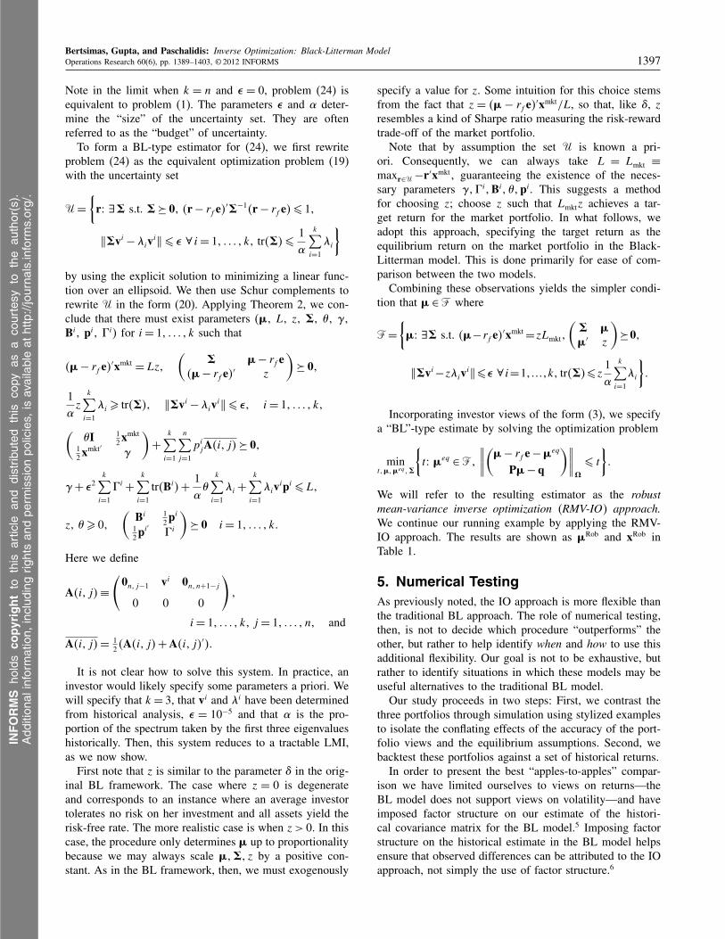
5.1.2. Market Perturbation. We next consider ascenario where future asset returns are drawn from a dis-tribution whose covariance matrix differs from the his-torical covariance matrix by a small, random additiveperturbation.7 Mean returns are then generated accordingto the CAPM. This scenario is consistent with a factormodel. Viewed as functions of this random perturbation, theportfolio’s risk and return are random variables. Approxi-mate densities for the portfolio return and portfolio standarddeviation are shown in Figure 1. We have taken q = 5.

The returns of the two IO portfolios have similar den-sities. They are better on average and more concentrated

INFORMS

holds

copyrightto

this

article

and

distrib

uted

this

copy

asa

courtesy

tothe

author(s).

Add

ition

alinform

ation,

includ

ingrig

htsan

dpe

rmission

policies,

isav

ailableat

http://journa

ls.in

form

s.org/.


Figure 1. Comparative performance of BL and MV-IO portfolios after a small perturbation in the covariance matrix.

5.0 12 13 14 15 16 17 18

Std dev (annualized %)

0

0.5

1.0

1.5

2.0

2.5

3.0

3.5

4.54.0

Return (annualized %)

Approximate density of returns Approximate density of portfolio std

BLMV-IORMV-IO

3.50

1

2

3

4

5

6

Note. The view q = 5.

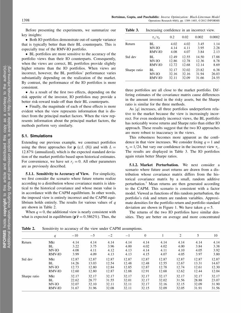
around their means than the BL portfolio. The standarddeviations of the IO portfolios are also smaller on aver-age and have thinner tails than the BL portfolio. Interest-ingly, the returns for all three portfolios are highly correlatedwith the realization of the view portfolio. In Figure 2 wehave plotted the excess returns over the market portfoliofor each approach as a function of the accuracy of theview p′r− q. The BL portfolio demonstrates a strongerdependence. In scenarios where the view is more correct(i.e., p′r− q ≈ 0), the BL approach outperforms the IOapproaches. For these data, however, such scenarios arevery rare.

Figure 2. Dependence of portfolio return on accuracyof the view.

To better understand this linear dependence, we computethe slope of a regression line for each set of returns as afunction of the view realization. We provide some resultsin Table EC.4 of the e-companion. Overall, the slope isgenerally positive when q > p′r, i.e., the view predicts p toperform better than it would in equilibrium, and increasingin magnitude in both the confidence �1/�0 and the extrem-ity �q−p′r�. In He and Litterman (1999), the authors provethese assertions formally for the BL model with a singleview under approximation (6). Our numerical study sug-gests that similar statements hold, at least approximately,for the MV-IO and RMV-IO approaches, but that the depen-dence is more mild. This insight will provide strong intu-ition when backtesting against a historical data set.

Finally, a more complete picture of the dependence on qas can be seen in Table EC.5 in the e-companion, wherewe have summarized portfolio characteristics after 10,000simulations.

5.1.3. Sensitivity to Choice of Portfolio p. We nextconsider a different view portfolio:

p′=[

20%�0%�10%�10%�10%�10%�10%�

− 10%�20%�20%]

�

Intuitively, the difference between p and p is that pdescribes information distinct from the information in theprinciple market factors, whereas p describes informationsimilar to the information in the principle market factors.More formally, the projection of p onto the space spannedby the first three eigenvectors of � is small, whereas theprojection of p onto the same space is large. Specifically,

�proj�p�< v1�v2�v3 >��

�p�≈ 2%�

�proj�p�< v1�v2�v3 >��

�p�≈ 84%�

INFORMS

holds

copyrightto

this

article

and

distrib

uted

this

copy

asa

courtesy

tothe

author(s).

Add

ition

alinform

ation,

includ

ingrig

htsan

dpe

rmission

policies,

isav

ailableat

http://journa

ls.in

form

s.org/.


where v1�v2�v3 are the three largest eigenvalues of �.Because both IO approaches constrain the eigenvectors ofthe covariance matrix to be close to their historical values,we expect that the extra degrees of freedom afforded tothem in fitting the covariance matrix are not helpful in real-izing this view. All three approaches must attempt to realizethe view by adjusting the estimate of the mean return awayfrom the CAPM equilibrium. Consequently, the portfoliosperform similarly. We display some illustrative results inTable EC.6 of the e-companion. Note that the ratio of port-folio return to standard deviation is nearly identical for allmethods.

5.2. Backtesting

We consider a data set of Morgan Stanley Composite Index(MSCI) sector indices from June ’92 to Dec ’09 with thethree-month U.S. Treasury bill as a proxy for the risk-freerate. For each month beginning with June ’98, we use theprevious 60 months of historical data to fit an empiricalcovariance matrix and use that month’s market capitaliza-tion across the sectors to compute the BL, MV-IO, andRMV-IO portfolios. Portfolios are constructed to have a tar-get annualized standard deviation L= 15�73%. We includethe Markowitz portfolio with this target standard deviationin our results for comparison.

To emphasize the differences between the methods, wechoose a single portfolio view over the entire time horizon,namely, p defined by (8). Recall that for a portfolio thatlives in the space spanned by the first three eigenvectors ofthe covariance matrix, the performance of all three meth-ods is quite similar. The percentage of p that lives in thisspace ranges from 5%–40%. This percentage and the real-ized returns for this portfolio are plotted in Figure EC.1 ofthe e-companion. The average realized monthly return forp is 0.03 %.

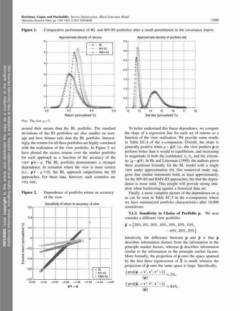
5.2.1. Static Views. We first consider the performanceof the portfolios when q is the same fixed constant eachperiod. This is a particularly crude belief, but in some ways

Figure 3. Portfolio characteristics for static views (June ’98–December ’09).

1510

Portfolio view q (%)

50–5–10–15 1510


50–5–10–15 1510

Portfolio view q (%)50–5–10–15

–2

–1

0

1

2

3

Ann

ualiz

ed (

%)

Ann

ualiz

ed (

%)

Ann

ualiz

ed (

%)4

5

6Average return Overall std dev Maximum std dev

BL23

22

21

20

19

18

17

16

15

40

42

38

36

34

32

30

28

26

24

MV-IORMV-IO

Notes. For comparison, the Markowitz portfolio has an average return of 0.00%, an overall standard deviation of 21.07%, and a maximal standard deviationof 36.17%.

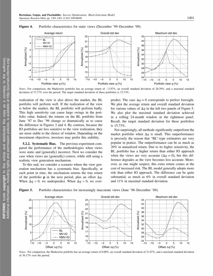
it is the best way to disassociate the performance of themethods from the system generating the views. We cal-culate the mean return and standard deviation experiencedover the data set. We plot these metrics in the left two pan-els of Figures 3. To better understand the risk experiencedwithin the period, we also compute the maximal standarddeviation achieved over a rolling window of 24 months,plotted in the rightmost panel of Figure 3.

The results for standard deviation and risk are quite strik-ing. For almost all values of q, the IO portfolios adopt lessrisk than the BL portfolio. Indeed, the difference betweenthe BL approach and the RMV-IO approach can be as greatas 6% for overall standard deviation and 11% for maximalstandard deviation. These results are intuitive because bothIO approaches allow a more flexible volatility estimation,and the RMV-IO approach, in particular, protects againstworst-case realizations of volatility. Recall that the targetstandard deviation for these portfolios was 15.73%, so thatthe IO portfolios more accurately match the target.

The results for the average return, however, are moresubtle. When q = 0, the view is almost in accordancewith equilibrium, and all three portfolios perform simi-larly to the Markowitz portfolio. One might be tempted toinfer that for q < 0 the BL significantly outperforms theIO approaches, whereas for q > 0, it underperforms. Thisinference, though, heavily depends on the choice of out-of-sample window. Compare Figure 3 with Figure 4, wherewe have performed the same experiment, but only aver-aged over the period Dec. ’99–Dec. ’09 (a difference of 18months). The average return of the BL portfolio demon-strates a very different dependence on q. By contrast, theaverage return of the IO portfolios and the standard devia-tion of all three portfolios is still quite similar.

We feel that this difference can at least partially beexplained by our insights from §5.1.2. Because the BLportfolio is very sensitive to the realization of the view,the portfolio may experience very large gains and losses.For example, suppose the view predicts p to perform muchbetter than it would in equilibrium, i.e., q � pT r. If the

INFORMS

holds

copyrightto

this

article

and

distrib

uted

this

copy

asa

courtesy

tothe

author(s).

Add

ition

alinform

ation,

includ

ingrig

htsan

dpe

rmission

policies,

isav

ailableat

http://journa

ls.in

form

s.org/.


Figure 4. Portfolio characteristics for static views (December ’99–December ’09).

1510


50–5–10–15 1510


50–5–10–15 1510

Portfolio view q (%)50–5–10–15

–6

–4

–2

Ann

ualiz

ed (

%)

Ann

ualiz

ed (

%)

Ann

ualiz

ed (

%)

2

0

4

6Average return Overall std dev Maximum std dev

BL22

21

20

19

18

17

16

15

14

40

42

38

36

34

32

30

28

26

24

MV-IORMV-IO

Notes. For comparison, the Markowitz portfolio has an average return of −2�97%, an overall standard deviation of 20.29%, and a maximal standarddeviation of 37.17% over the period. The target standard deviation of these portfolios is 15.73%.

realization of the view is also above the market, the BLportfolio will perform well. If the realization of the viewis below the market, the BL portfolio will perform badly.This high sensitivity can cause large swings in the port-folio value. Indeed, the returns on the BL portfolio fromJune ’97 to Dec ’99 change so dramatically as to causethe difference in Figures 3 and 4. By contrast, because theIO portfolios are less sensitive to the view realization, theyare more stable to the choice of window. Depending on theinvestment objectives, investors may prefer this stability.

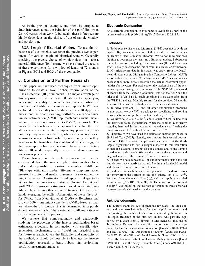
5.2.2. Systematic Bias. The previous experiment com-pared the performance of the methodologies when viewswere static and (generally) incorrect. Next we consider thecase when views are (generally) correct, while still using arealistic view generation mechanism.

To this end, we consider a scenario where the view gen-eration mechanism has a systematic bias. Specifically, ateach point in time, the mechanism returns the true returnof the portfolio p in the next period, plus an offset �q.When �q < 0, we underpredict. When �q > 0, we over-

Figure 5. Portfolio characteristics for increasingly inaccurate views (June ’98–December ’09).

Average return Overall std dev Maximum std dev

Offset ∆q (%) Offset ∆q (%)

Ann

ualiz

ed (

%)

Ann

ualiz

ed (

%)

Ann

ualiz

ed (

%)

151050–5–10–15

Offset ∆q (%)

151050–5–10–15151050–5–10–15

BLMV-IORMV-IO

24

16

17

18

19

20

0

5

10

15

20

25

21

22

23

15

40

42

44

38

36

34

32

30

28

26

24

Notes. For comparison, the Markowitz portfolio has an average return of 0.00%, an overall standard deviation of 21.07%, and a maximal standard deviationof 36.17% over the period.

predict. The case �q = 0 corresponds to perfect foresight.We plot the average return and overall standard deviationfor various values of �q in the left two panels of Figure 5.We also plot the maximal standard deviation achievedin a rolling 24-month window in the rightmost panel.Recall, the target standard deviation for these portfoliosis 15.73%.

Not surprisingly, all methods significantly outperform themarket portfolio when �q is small. This outperformanceis precisely the reason that “BL”-type estimators are verypopular in pratice. The outperformance can be as much as20% in annualized return. Due to its higher sensitivity, theBL portfolio has a higher return than either IO approachwhen the views are very accurate (�q = 0), but this dif-ference degrades as the view becomes less accurate. More-over, as one might suspect, this extra return comes at thecost of increased risk. The BL model generally adopts morerisk than either IO approach. The difference can be quitesubstantial, as much as 6% in overall standard deviationand 11% in maximal standard deviation.

INFORMS

holds

copyrightto

this

article

and

distrib

uted

this

copy

asa

courtesy

tothe

author(s).

Add

ition

alinform

ation,

includ

ingrig

htsan

dpe

rmission

policies,

isav

ailableat

http://journa

ls.in

form

s.org/.


As in the previous example, one might be tempted todraw inferences about the behavior of the portfolios whenãq < 0 versus when ãq > 0, but again, these inferences arehighly dependent on the choice of out-of-sample windowand portfolio p.

5.2.3. Length of Historical Window. To test the ro-bustness of our insights, we reran the previous two exper-iments for various lengths of historical window. Generallyspeaking, the precise choice of window does not make amaterial difference. To illustrate, we have plotted the resultsof these experiments for a window of length of 72 monthsin Figures EC.2 and EC.3 of the e-companion.

6. Conclusion and Further ResearchIn this paper we have used techniques from inverse opti-mization to create a novel, richer, reformulation of theBlack-Litterman (BL) framework. The major advantage ofthis approach is the increased flexibility for specifyingviews and the ability to consider more general notions ofrisk than the traditional mean-variance approach. We haveexploited this flexibility to introduce two new BL-type esti-mators and their corresponding portfolios, a mean-varianceinverse optimization (MV-IO) approach and a robust mean-variance inverse optimization (RMV-IO) approach. Themajor distinction between the approaches is that the firstallows investors to capitalize upon any private informa-tion they may have on volatility, whereas the second seeksto insulate investors from volatility uncertainty when theyhave no such information. Computational evidence suggeststhat these approaches provide certain benefits over the tra-ditional BL model, especially in scenarios where views arenot known precisely.

These two are not the only estimators that can beconstructed from the inverse optimization methodology.Indeed, it is possible to construct a number of different“BL”-type estimators under different assumptions aboutinvestor behavior and market dynamics. For example, onemight frame an IO estimator based upon shrinkage tech-niques for the covariance matrix (following Ledoit andWolf 2003). Shrinkage estimators have demonstrated sig-nificant benefits in other areas of finance. On the otherhand, leveraging the explicit formulation of the set U4�1�5for CVaR� from Natarajan et al. (2009) or Bertsimas andBrown (2009), one might consider a CVaR�-based estima-tor where the distribution of r is determined in a purelydata-driven way. Each of these estimators will enjoy its ownparticular numerical properties.

We believe that computationally and analyticallystudying the properties of the inverse-optimization basedestimators, especially in conjunction with specific viewgeneration mechanisms, is a fruitful and practical areafor future research. Given the flexibility and simplicity ofthe method, it should be possible to leverage the inverseoptimization approach to build robust, high-performingportfolio investment strategies.

Electronic Companion

An electronic companion to this paper is available as part of theonline version at http://dx.doi.org/10.1287/opre.1120.1115.

Endnotes

1. To be precise, Black and Litterman (1992) does not provide anexplicit Bayesian interpretation of their result, but instead relieson Thiel’s Mixed Estimation Theorem. We do not know who wasthe first to recognize the result as a Bayesian update. Subsequentresearch, however, including Litterman’s own (He and Litterman1999), usually describes the initial result in a Bayesian framework.2. Historical return data in this paper was drawn from the DataS-tream database using Morgan Stanley Composite Indices (MSCI)sector indices as proxies. We chose to use MSCI sector indicesbecause they more closely resemble the actual investment oppor-tunities for investors. For each sector, the market share of the sec-tor was proxied using the percentage of the S&P 500 composedof stocks from that sector. Constituent lists for the S&P and theprice and market share for each constituent stock were taken fromthe WRDS database. Monthly returns for the previous 24 monthswere used to construct volatility and correlation estimates.3. To solve problem (13) and all other optimization problemsin this paper, we use CVX, a package for specifying and solvingconvex optimization problems (Grant and Boyd 2010).4. We have set k = 3, � = 10−8, and � equal to 87% in line withthe historical value. Furthermore, when the solution è is nearlysingular, here and in the remainder, we calculate xMV using thepseudo-inverse of è with a tolerance of 5 × 10−4.5. Specifically, we have used the estimation method proposed in§9.5.1 of Tsay (2005). Namely, we truncate the spectral decom-position of the traditional sample covariance matrix at the third-largest eigenvalue and add a diagonal matrix to this truncationso that the diagonal elements of our estimate and of the samplecovariance matrix match. We use this sum of the truncation anddiagonal matrix as the estimate è in the BL model.6. In fact, we have repeated all of our experiments using the fullsample covariance matrix and a rank 3 estimator for the BL modeland obtained similar results in both cases.7. In detail, for each scenario we generate 10 random vectorsuniformly from the surface of the unit sphere, say v11 0 0 0 1v10.We then form the matrix E =

∑10i=1 v

ivi′ and apply the scaledperturbation 445 × 10−35/trace4E55E. The choice of the constant5 × 10−3 was based on the average difference in trace observedbetween covariance matrices in the data set.

Acknowledgments

The authors thank the two anonymous reviewers, the area edi-tor, and the associate editor for the helpful comments andfor pointing the authors toward some interesting literature onthe topic. Research of the first two authors was partially sup-ported by a grant from Citigroup to Massachusetts Institute ofTechnology. Research for the third author was partially sup-ported by the National Science Foundation [Grants EFRI-0735974and IIS-1237022], the Department of Energy [Grant DE-FG52-06NA27490], the Office of Naval Research [Grant N00014-10-1-0952], the National Institute of General Medical Sciences [GrantGM093147], and the Army Research Office [Grants W911NF-11-1-0227 and 61789-MA-MUR].

INFORMS

holds

copyrightto

this

article

and

distrib

uted

this

copy

asa

courtesy

tothe

author(s).

Add

ition

alinform

ation,

includ

ingrig

htsan

dpe

rmission

policies,

isav

ailableat

http://journa

ls.in

form

s.org/.


ReferencesAhuja RK, Orlin JB (2001) Inverse optimization. Oper. Res.

49(5):771–783.Artzner P, Delbaen F, Eber JM, Heath D (1999) Coherent measures of

risk. Math. Finance 9(3):203–228.Ben-Tal A, Nemirovski A (2008) Selected topics in robust convex opti-

mization. Math. Programming 112(1):125–158.Bertsekas DP (1999) Nonlinear Programming (Athena Scientific,

Belmont, MA).Bertsimas D, Brown DB (2009) Constructing uncertainty sets for robust

linear optimization. Oper. Res. 57(6):1483–1495.Bertsimas D, Brown DB, Caramanis C (2011) Theory and applications of

robust optimization. SIAM Rev. 53:464–501.Bertsimas D, Lauprete GJ, Samarov A (2004) Shortfall as a risk measure:

Properties, optimization and applications. J. Econom. Dynam. Control28(7):1353–1381.

Bevan A, Winkelmann K (1998) Using the Black-Litterman Global AssetAllocation Model: Three years of practical experience. Fixed IncomeResearch, Goldman Sachs & Company, New York.

Black F, Litterman R (1992) Global portfolio optimization. Financial Ana-lysts J. 48(5):28–43.

Boyd SP, Vandenberghe L (2004) Convex Optimization (CambridgeUniversity Press, New York).

Connor G, Korajczyk RA (1995) The arbitrage pricing theory andmultifactor models of asset returns. Jarrow RA, Maksimovic V,Ziemba WT, eds. Finance. Handbooks in Operations Research andManagement Science, Vol. 9 (Elsevier, Amsterdam), 87–144.

Da Silva AS, Lee W, Pornrojnangkool B (2009) The Black-Littermanmodel for active portfolio management. J. Portfolio Management35(2):61–70.

Fama EF, French KR (1993) Common risk factors in the returns on stocksand bonds. J. Financial Econom. 33(1):3–56.

Giacometti R, Bertocchi M, Rachev ST, Fabozzi FJ (2007) Stable distri-butions in the Black–Litterman approach to asset allocation. Quant.Finance 7(4):423–433.

Grant M, Boyd S (2010) CVX: Matlab software for disciplined con-vex programming, version 1.21. Accessed April 1, 2011, http://cvxr.com/cvx.

Grootveld H, Hallerbach W (1999) Variance vs. downside risk. Eur. J.Oper. Res. 114(2):304–319.

Harlow WV (1991) Asset allocation in a downside-risk framework. Finan-cial Analysts J. 47(5):28–40.

He G, Litterman R (1999) The intuition behind Black-Litterman modelportfolios. Investment Management Research, Goldman Sachs &Company, New York.

Herold U (2005) Computing implied returns in a meaningful way. J. AssetManagement 6(1):53–64.

Heuberger C (2004) Inverse combinatorial optimization: A survey onproblems, methods, and results. J. Combin. Optim. 8(3):329–361.

Iyengar G, Kang W (2005) Inverse conic programming with applications.Oper. Res. Lett. 33(3):319–330.

Jorion P (1997) Value at Risk: The New Benchmark for Controlling MarketRisk (McGraw-Hill, New York).

Krishnan HP, Mains NE (2005) The two-factor Black-Litterman model.Risk (July).

Ledoit O, Wolf M (2003) Improved estimation of the covariance matrix ofstock returns with an application to portfolio selection. J. EmpiricalFinance 10(5):603–621.

Martellini L, Ziemann V (2007) Extending Black-Litterman analysisbeyond the mean-variance framework. J. Portfolio Management33(4):33–44.

Meucci A (2005) Beyond Black-Litterman: Views on non-normal markets.http://ssrn.com/abstract=848407.

Meucci A (2008) Fully flexible views: Theory and practice. Risk21(10):97–102.

Meucci A, Ardia D, Keel S (2011) Fully flexible views in multivariatenormal markets. http://ssrn.com/abstract=1742559.

Natarajan K, Pachamanova D, Sim M (2009) Constructing risk measuresfrom uncertainty sets. Oper. Res. 57(5):1129–1141.

Pástor L (2000) Portfolio selection and asset pricing models. J. Finance55(1):179–223.

Pástor L, Stambaugh RF (2000) Comparing asset pricing models: Aninvestment perspective. J. Financial Econom. 56(3):335–381.

Rockafellar RT, Uryasev S (2002) Conditional value-at-risk for generalloss distributions. J. Banking Finance 26(7):1443–1471.

Sharpe WF (1964) Capital asset prices: A theory of market equilibriumunder conditions of risk. J. Finance 19(3):425–442.

Tsay RS (2005) Analysis of Financial Time Series, 2nd ed. (Wiley-Interscience, Hoboken, NJ).

Walters J (2010) The Black-Litterman model: A detailed exploration.Accessed January 1, 2011, http://www.blacklitterman.org.

Dimitris Bertsimas is the Boeing Professor of OperationsResearch, co-director of the Operations Research Center at Mas-sachusetts Institute of Technology, and a member of the NationalAcademy of Engineering. He works on optimization, appliedprobability, and data mining and their applications. The paper inthis issue is part of the author’s research program in understandingthe implications of inverse optimization in a variety of fields.

Vishal Gupta is a Ph.D. candidate in operations research atMassachusetts Institute of Technology under the supervision ofDimitris Bertsimas. Prior to matriculating at MIT, he spent sev-eral years working in the financial industry. Broadly speaking,he is interested in developing tractable paradigms for modelinguncertainty.

Ioannis Ch. Paschalidis is a professor and Distinguished Fac-ulty Fellow in the College of Engineering at Boston Universitywith a joint appointment in the Department of Electrical and Com-puter Engineering and the Division of Systems Engineering. He isco-director of the Center for Information and Systems Engineer-ing (CISE). His current research interests lie in the fields of sys-tems and control, networking, applied probability, optimization,operations research, computational biology, and bioinformatics.

INFORMS

holds

copyrightto

this

article

and

distrib

uted

this

copy

asa

courtesy

tothe

author(s).

Add

ition

alinform

ation,

includ

ingrig

htsan

dpe

rmission

policies,

isav

ailableat

http://journa

ls.in

form

s.org/.

inverse optimization: a new perspective on the black ...dbertsim/papers/finance/inverse optimization...

Documents