1  

Inverse Prediction and Optimization of Flow Control Conditions

for Confined Spaces using a CFD-Based Genetic Algorithm Yu Xue1, Zhiqiang (John) Zhai1, 2*, Qingyan Chen1, 3 1School of Environmental Science and Engineering, Tianjin University, Tianjin 300072, China 2University of Colorado at Boulder, Boulder, CO, 80309, USA 3School of Mechanical Engineering, Purdue University, IN 47905, USA *Corresponding email: john.zhai@colorado.edu Abstract Optimizing an indoor flow pattern according to specific design goals requires systematic evaluation and prediction of the influences of critical flow control conditions such as flow inlet temperature and velocity. In order to identify the best flow control conditions, conventional approach simulates a large number of flow scenarios with different boundary conditions. This paper proposes a method that combines the genetic algorithm (GA) with computational fluid dynamics (CFD) technique, which can efficiently predict and optimize the flow inlet conditions with various objective functions. A coupled simulation platform based on GenOpt (GA program) and Fluent (CFD program) was developed, in which the GA was improved to reduce the required CFD simulations. A mixing convection case in a confined space was used to evaluate the performance of the developed program. The study shows that the method can predict accurately the inlet boundary conditions, with given controlling variable values in the space, with fewer CFD cases. The results reveal that the accuracy of inverse prediction is influenced by the error of CFD simulation that need be controlled within 15%. The study further used the Predicted Mean Vote (PMV) as the cost function to optimize the inlet boundary conditions (e.g., supply velocity, temperature, and angle) of the mixing convection case as well as two more realistic aircraft cabin cases. It presents interesting optimal correlations among those controlling parameters. Keywords: Inverse Modeling, Flow Control, Confined Space, Computational Fluid Dynamics, Genetic Algorithm, Aircraft Cabin Introduction With rapid developments in fluid dynamics, numerical science and computer technologies, computational fluid dynamics (CFD) has become an efficient tool for indoor environment study and system design. Optimizing an indoor flow pattern according to specific design goals requires systematic evaluation and prediction of the influences of critical flow control conditions such as flow inlet temperature, velocity and angle. In order to identify the best flow control conditions, conventional approach simulates a large number of flow scenarios with different boundary conditions. Previous studies reveal advanced search and optimization algorithms such as genetic algorithm (GA) can effectively reduce the total number of iterations to reach an (or a group of) optimal solution(s) [1]. GA is an optimization algorithm that simulates natural evolution in the search of optimal solutions [2]. It has been applied to a variety of engineering design, parameter identification and system optimization. Efforts of

Xue, Y., Zhai, Z., and Chen, Q. 2013. “Inverse prediction and optimization of flow control conditions for confined spaces using a CFD-based genetic algorithm,” Building and Environment,64, 77-84.

2  

coupling GA with CFD, however, were mostly on the optimization of exterior geometries of various objects. For instance, Obayashi and Takanashi [3] combined GA with CFD to optimize the target pressure distributions of an airfoil. Other examples include the shape design of cars [4], melt blowing slot die [5], and transition piece [6]. Malkawi et al. [7] used the CFD-based GA method to search the optimal room size and ventilation system which can satisfy both thermal and ventilation requirements. The study was for a relatively simple case and did not evaluate the influence of CFD prediction error on optimal design. Kato and Lee [8] applied a similar approach to optimizing a hybrid air-conditioning system with natural ventilation. The study aimed at minimizing the energy consumption of the mechanical systems. The study developed a two-step method to reduce the computing effort. Optimal results were acquired first with a coarse CFD mesh, which were then refined with a fine mesh for detailed analyses. It should be noted that CFD results with coarse meshes may produce incorrect flow field which can lead to wrong optimal results. Zhou and Haghighat [9][10] employed the artificial neural network (ANN) to reduce the modeling time; however, training the ANN still requires a great number of CFD cases for individual projects. This study develops a general simulation tool by integrating GA and CFD programs. The tool can inversely predict control conditions based on limited experiment data of indoor flow field. It can also be used to optimize various control conditions of indoor flows under different objective functions (PMV in this paper). The tested control conditions include supply velocity (vector) and temperature of flow inlet, etc. Locally optimal solutions and multiple solutions may exist for multivariable optimization problems, where the GA presents the special strength in capturing the global optimal results and multiple solutions. Methodologies Modified Genetic Algorithm There are generally two categories of optimization algorithms: gradient-based method and gradient-free method. Gradient-based methods cannot deal with nonlinear problems well [11] and can be easily trapped in local optimal values [12]. Airflow and heat transfer problems in confined spaces are highly nonlinear and thus require the utilization of gradient-free methods. As one of the gradient-free methods, genetic algorithm is capable of resolving nonlinear and multi-solution problems, requiring less computing time to find global optimum than other methods [13]. Genetic algorithm uses evolution operations to generate new populations with higher average fitness values [14]. The higher fitness value an individual possesses, the closer it is to the optimal result. A typical GA procedure breaks down as follows: (1) Generate a random initial population of potential solutions, which contains several

individuals; (2) Evaluate the fitness value of each individual with specified cost function; (3) Check whether the population meets the prescribed optimization criterion; if not, apply

genetic operations such as selection, crossover, and mutation to the population to create a new generation of potential solutions;

(4) Repeat step (2) and (3) until the optimization criterion is met.

3  

Initial Population

Fitness value

Satisfy stopping criteria?

Optimal results

New population

Individuals  satisfying demand

Selection

Crossover

MutationCost 

Function

Coding

Decoding

Tournament selection

Multi‐point crossover

Mutation Operator

Y

N

Curve Fitting

Evolution

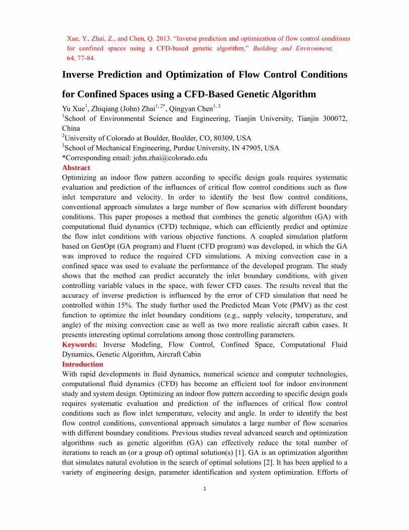
Fig.1 Flowchart of the modified GA

The standard GA encounters several challenges when used for indoor environments. In the procedure of coding, a basic genetic algorithm usually encodes multi-variables into one long binary code. This requires large computing memory and resource for a multi-variable case. With all of variables coded in one long code, a standard GA crossovers code of each individual at one or several points randomly. This is a totally random procedure that is good for variation but discourages the convergence approaching optimum(s). The standard GA often use the roulette wheel selection method to choose suitable parents for creating next population, implying that the higher fitness value an individual has, the higher probability it will be chosen as a parent to create the new generation of individuals. This may be suitable for individuals with a large fitness value difference, but may illustrate the character of random selection and lose the benefits of evolution when the differences are marginal. Airflow and heat transfer in confined spaces involve multi-variables. These variables can have continuous changes, and may lead to small differences in fitness values among individuals. Indeed, most inverse prediction and optimization problems for indoor environment may involve subtle fine-tuning of critical flow control conditions. Hence, the standard GA need be improved to ensure a better convergence. The study improves the coding, selection and crossover procedure to accelerate the optimization convergence speed and reduce the computing effort (as highlighted in Fig. 1). For the coding, various variables were encoded and managed independently. This made it easy to conduct GA operations on each of them. For the selection, the roulette wheel selection method was replaced by the tournament-selection-method, which works as follows: (1) Pick out m individuals randomly from the current population (containing n individuals) to

form a subset, where 2≦m<n; (2) Identify the individual with the highest fitness value from the subset as one of the parents; (3) Repeat the step (1) and (2) until n individuals are obtained (allow repeated individuals in

the selected n individuals).

4  

The obtained n individuals form the parent population that will be used to generate a new population with crossover and mutation. In this way, individuals with a higher fitness value will be chosen even if there are little differences between any two individuals. In addition, at least m-1 individuals with the lowest fitness values will be rejected, which makes it possible to balance the optimization convergence speed and the global search capability of the algorithm. For the crossover, a so-called “the only son crossover method” was developed: (1) Select an individual from the parent population randomly as the primary parent, then

chose another parent randomly; (2) Crossover at one point randomly for every independent variable, so the code of each

variable is divided into two parts: high-order part and low-order part. The high-order part of the code shows the main features of a variable;

(3) Generate a son of the parents with the high-order part of the primary parent and the low-order part of the other parent. So the son will inherit more features from the primary parent;

(4) Repeat the step (1) to (3) until n son individuals are obtained; then after mutation, they form the new generation of population.

These modifications above will substantially accelerate the convergence because every step in the procedure contributes to the creation of a new generation with a higher average fitness value. Besides excellent capability in the global optimization, GA is also suitable for developing regression correlations when applied to multi-solution problems [15][16]. Regression with curve-fitting requires adequate optimal points to demonstrate the curve trend, implying a large amount of computing time. If the expression of a curve is known in prior, the curves can be fitted with few points. This study finds an approach to effectively predicting the form of correlation curves: an independent population is arranged to collect global optimal individuals, and optimization process stops when every individual of this independent population meets the requirement of the regression. Integration of GA-CFD A coupled computational platform based on GenOpt [17] and Fluent [18] was developed to implement the integration of GA and CFD. GenOpt is a generic optimization program that can be used to minimize an objective function computed by a simulation tool, using text files for input and output. Fluent is one of the popular commercial CFD software that can start and input parameters with text files. The study used Gambit (the pre-processing tool of Fluent) to establish computer models of indoor environments. The modified GA was programmed into GenOpt. An interface was developed to transfer files and data among GenOpt, Gambit and Fluent, fundamentally integrating these programs into one simulation platform.

5  

Initial Population

Fitness value

Satisfy stopping criteria?

Optimal results

New population

Individuals satisfying 

demand level 

Selection

Crossover

Mutation

Y

N

Evolution

Boundary condition

（size, v, t, …）

Generate   Gambit.jou & Fluent.jou file

Run Gambit & Fluent 

simulation

Extract results

All individualssimulated?

YN

 

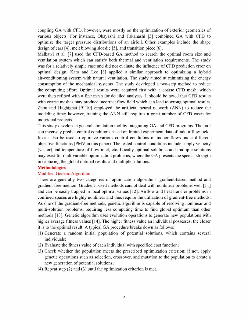
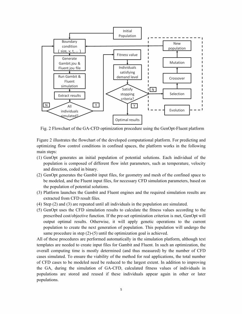
Fig. 2 Flowchart of the GA-CFD optimization procedure using the GenOpt-Fluent platform

Figure 2 illustrates the flowchart of the developed computational platform. For predicting and optimizing flow control conditions in confined spaces, the platform works in the following main steps: (1) GenOpt generates an initial population of potential solutions. Each individual of the

population is composed of different flow inlet parameters, such as temperature, velocity and direction, coded in binary.

(2) GenOpt generates the Gambit input files, for geometry and mesh of the confined space to be modeled, and the Fluent input files, for necessary CFD simulation parameters, based on the population of potential solutions.

(3) Platform launches the Gambit and Fluent engines and the required simulation results are extracted from CFD result files.

(4) Step (2) and (3) are repeated until all individuals in the population are simulated. (5) GenOpt uses the CFD simulation results to calculate the fitness values according to the

prescribed cost/objective function. If the pre-set optimization criterion is met, GenOpt will output optimal results. Otherwise, it will apply genetic operations to the current population to create the next generation of population. This population will undergo the same procedure in step (2)-(5) until the optimization goal is achieved.

All of these procedures are performed automatically in the simulation platform, although text templates are needed to create input files for Gambit and Fluent. In such an optimization, the overall computing time is mostly determined (and thus measured) by the number of CFD cases simulated. To ensure the viability of the method for real applications, the total number of CFD cases to be modeled need be reduced to the largest extent. In addition to improving the GA, during the simulation of GA-CFD, calculated fitness values of individuals in populations are stored and reused if these individuals appear again in other or later populations.

6  

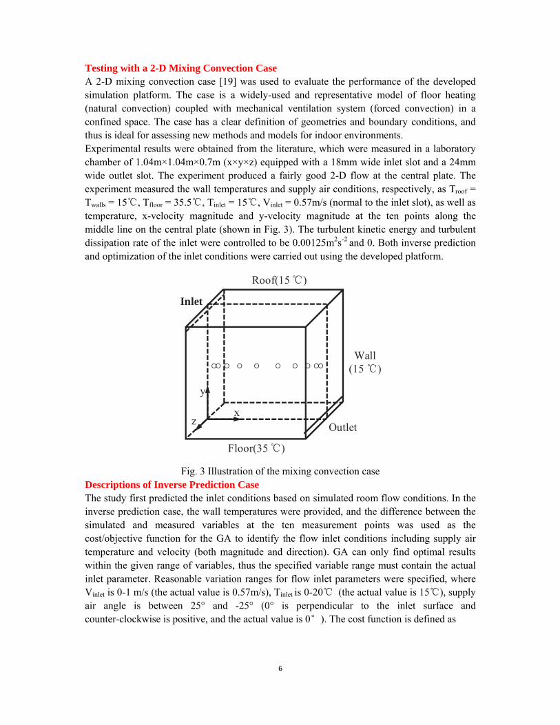
Testing with a 2-D Mixing Convection Case A 2-D mixing convection case [19] was used to evaluate the performance of the developed simulation platform. The case is a widely-used and representative model of floor heating (natural convection) coupled with mechanical ventilation system (forced convection) in a confined space. The case has a clear definition of geometries and boundary conditions, and thus is ideal for assessing new methods and models for indoor environments. Experimental results were obtained from the literature, which were measured in a laboratory chamber of 1.04m×1.04m×0.7m (x×y×z) equipped with a 18mm wide inlet slot and a 24mm wide outlet slot. The experiment produced a fairly good 2-D flow at the central plate. The experiment measured the wall temperatures and supply air conditions, respectively, as Troof = Twalls = 15℃, Tfloor = 35.5℃, Tinlet = 15℃, Vinlet = 0.57m/s (normal to the inlet slot), as well as temperature, x-velocity magnitude and y-velocity magnitude at the ten points along the middle line on the central plate (shown in Fig. 3). The turbulent kinetic energy and turbulent dissipation rate of the inlet were controlled to be 0.00125m2s-2 and 0. Both inverse prediction and optimization of the inlet conditions were carried out using the developed platform.

Inlet

Outlet

Roof(15 ℃)

Floor(35 ℃)

Wall(15 ℃)

x

y

z

 

Fig. 3 Illustration of the mixing convection case Descriptions of Inverse Prediction Case The study first predicted the inlet conditions based on simulated room flow conditions. In the inverse prediction case, the wall temperatures were provided, and the difference between the simulated and measured variables at the ten measurement points was used as the cost/objective function for the GA to identify the flow inlet conditions including supply air temperature and velocity (both magnitude and direction). GA can only find optimal results within the given range of variables, thus the specified variable range must contain the actual inlet parameter. Reasonable variation ranges for flow inlet parameters were specified, where Vinlet is 0-1 m/s (the actual value is 0.57m/s), Tinlet is 0-20℃ (the actual value is 15℃), supply air angle is between 25° and -25° (0° is perpendicular to the inlet surface and counter-clockwise is positive, and the actual value is 0°). The cost function is defined as

7  

,...102,1---

31

2

2'

2

2'

2

2'

iT

TTV

VV

VVV

Fi

ii

yi

yiyi

xi

xixi (1)

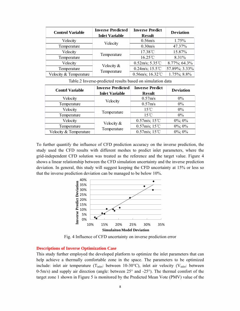
where F is the cost function value, V’xi and V’yi are the simulated velocity at the ten points, T’i is the simulated temperature at the ten points, Vxi, Vyi and Ti are the measured results. Smaller value of F represents higher fitness value and the simulation goal is to find the solution with the minimal F. Results of Inverse Prediction Case Table 1 presents the inverse predict results of seven cases, based on the difference between the simulated and measured results. The tested seven cases examined different combinations of control variables (values on the ten points) and inversely predicted inlet variables (values of the inlet), such as: (1) Predicting inlet velocity based on controlled velocity on the ten points; (2) Predicting inlet velocity based on controlled temperature on the ten points; (3) Predicting inlet temperature based on controlled velocity on the ten points; (4) Predicting both inlet temperature and velocity based on controlled velocity on the ten points, etc. The results show noticeable differences between the predicted and actual inlet conditions for the following cases (1) predicting inlet velocity based on controlled temperature on the ten points (47.37%); (2) predicting both inlet velocity and temperature based on controlled velocity on the ten points (mainly for temperature 64.3%); (3) predicting both inlet velocity and temperature based on controlled temperature on the ten points (mainly for velocity 57.89%). This can be understood by analyzing the governing equation (both the momentum and energy equations) of the flow. This mixing convection case has a stronger forced convection mechanism than the natural convection mechanism. Within the specified variation ranges of inlet parameters, the indoor temperature distribution is less sensitive to supply air velocity than to supply air temperature, while the indoor velocity distribution is more sensitive to supply air temperature than to supply air velocity and the distribution of indoor velocity is more sensitive to supply air velocity than to supply air temperature. Hence, predicting inlet velocity based on indoor velocity has a better accuracy than predicting inlet velocity based on indoor temperature. The difference between the simulated and measured control variables, which leads to the difference between the predicted and actual inlet conditions, are attributed to the errors inherent in both CFD simulation and experimental measurement. In order to verify the accuracy of the algorithm itself, these errors were eliminated by using the CFD simulation results with the actual inlet conditions as the reference (rather than the measurement) for the inverse prediction. Table 2 shows the inverse predict results under this ideal condition that excludes the influence of CFD and experiment uncertainties. The results reveal that the CFD-based GA program can precisely identify the actual inlet conditions. It is noticed that the modified GA reduces almost half of the computing time than the standard GA.

Table 1 Inverse-predicted results based on experiment data

8  

Control VariableInverse Predicted

Inlet VariableInverse Predict

ResultDeviation

Velocity 0.56m/s 1.75%Temperature 0.30m/s 47.37%

Velocity 17.38℃ 15.87%Temperature 16.25℃ 8.31%

Velocity 0.52m/s; 5.35℃ 8.77%; 64.3%Temperature 0.24m/s; 15.5℃ 57.89%; 3.33%

Velocity & Temperature 0.56m/s; 16.32℃ 1.75%; 8.8%

Velocity

Temperature

Velocity &Temperature

Table.2 Inverse-predicted results based on simulation data

Contrl Variable Inverse Predicted

Inlet VariableInverse Predict

ResultDeviation

Velocity 0.57m/s 0%Temperature 0.57m/s 0%

Velocity 15℃ 0%Temperature 15℃ 0%

Velocity 0.57m/s; 15℃ 0%; 0%Temperature 0.57m/s; 15℃ 0%; 0%

Velocity & Temperature 0.57m/s; 15℃ 0%; 0%

Velocity

Temperature

Velocity &Temperature

To further quantify the influence of CFD prediction accuracy on the inverse prediction, the study used the CFD results with different meshes to predict inlet parameters, where the grid-independent CFD solution was treated as the reference and the target value. Figure 4 shows a linear relationship between the CFD simulation uncertainty and the inverse prediction deviation. In general, this study will suggest keeping the CFD uncertainty at 15% or less so that the inverse prediction deviation can be managed to be below 10%.

 

0%

5%

10%

15%

20%

25%

30%

35%

40%

10% 15% 20% 25% 30% 35%Imve

rse

Pre

dic

t D

evia

tion

Simulaiton Model Deviation Fig. 4 Influence of CFD uncertainty on inverse prediction error

Descriptions of Inverse Optimization Case This study further employed the developed platform to optimize the inlet parameters that can help achieve a thermally comfortable zone in the space. The parameters to be optimized include: inlet air temperature (Tinlet: between 10-30°C), inlet air velocity (Vinlet: between 0-5m/s) and supply air direction (angle: between 25° and -25°). The thermal comfort of the target zone 1 shown in Figure 5 is monitored by the Predicted Mean Vote (PMV) value of the

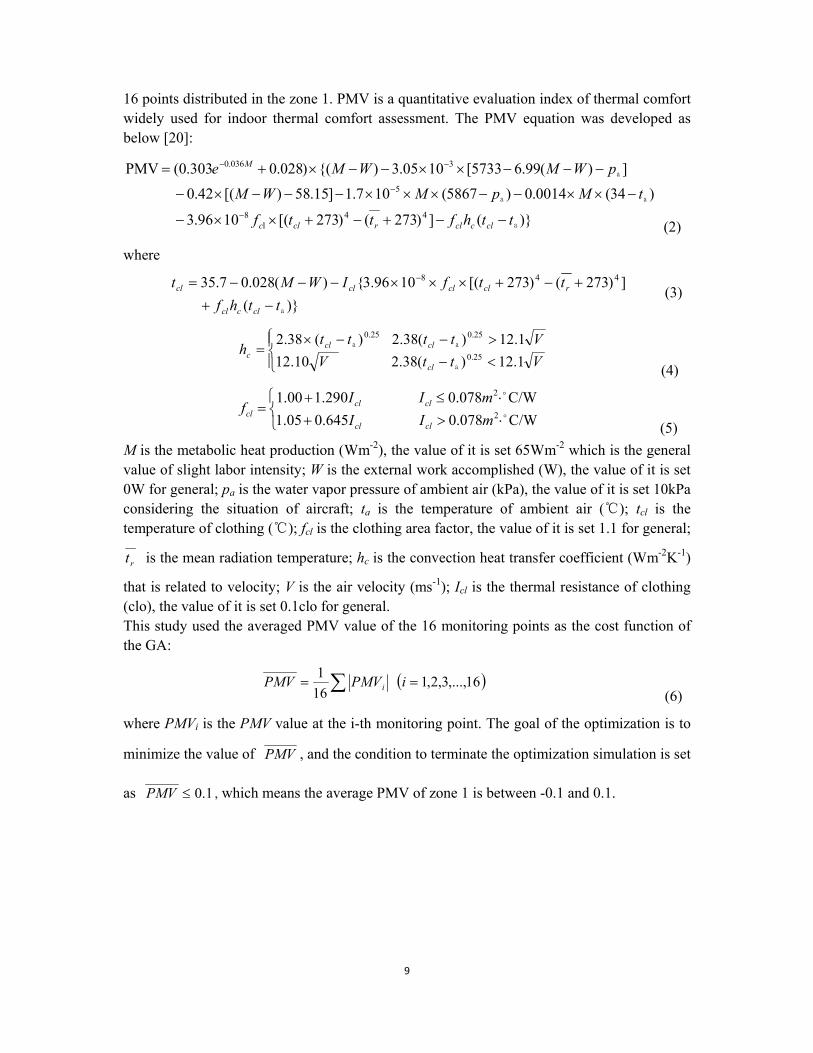
9  

16 points distributed in the zone 1. PMV is a quantitative evaluation index of thermal comfort widely used for indoor thermal comfort assessment. The PMV equation was developed as below [20]:

)}(])273()273[(1096.3

)34(0014.0)5867(107.1]15.58)[(42.0])(99.65733[1005.3){()028.0303.0(PMV

44l

8

5

3036.0

а

аа

а

tthfttf

tMpMWMpWMWMe

clcclrclc

M

(2)

where

)}(])273()273[(1096.3{)(028.07.35 448

аtthfttfIWMt

clccl

rclclclcl

(3)

VttVVtttt

hcl

clclc 1.12)(38.210.12

1.12)(38.2)(38.225.0

25.025.0

а

аа

(4)

C/W078.0645.005.1C/W078.0290.100.1

2

2

mIImII

fclcl

clclcl

(5) M is the metabolic heat production (Wm-2), the value of it is set 65Wm-2 which is the general value of slight labor intensity; W is the external work accomplished (W), the value of it is set 0W for general; pa is the water vapor pressure of ambient air (kPa), the value of it is set 10kPa considering the situation of aircraft; ta is the temperature of ambient air (℃); tcl is the temperature of clothing (℃); fcl is the clothing area factor, the value of it is set 1.1 for general;

rt is the mean radiation temperature; hc is the convection heat transfer coefficient (Wm-2K-1)

that is related to velocity; V is the air velocity (ms-1); Icl is the thermal resistance of clothing (clo), the value of it is set 0.1clo for general. This study used the averaged PMV value of the 16 monitoring points as the cost function of the GA:

16,...,3,2,1161

iPMVPMV i                                                      (6)

where PMVi is the PMV value at the i-th monitoring point. The goal of the optimization is to

minimize the value of PMV , and the condition to terminate the optimization simulation is set

as 0.1PMV , which means the average PMV of zone 1 is between -0.1 and 0.1. 

10  

x

y

z

Inlet

Outlet

Roof(15 ℃)

Floor(35 ℃)

Wall(15 ℃)

1

Fig. 5 Optimization of inlet conditions based on the thermal comfort criterion in Zone 1

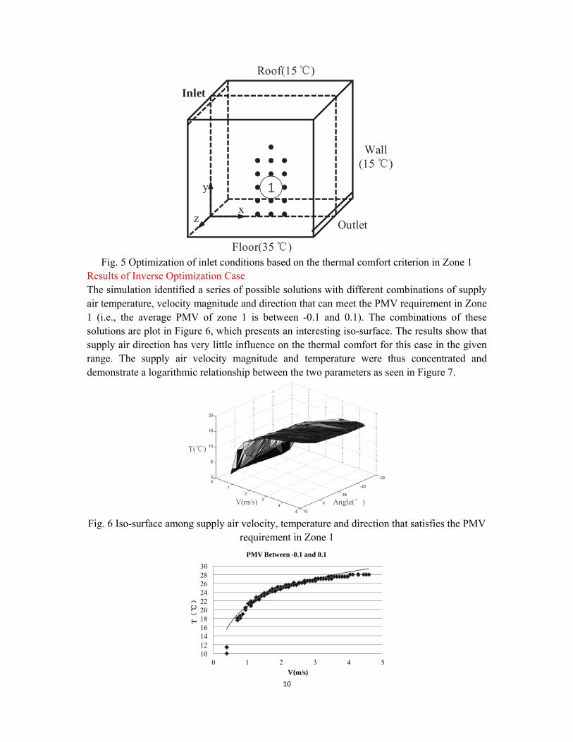
Results of Inverse Optimization Case The simulation identified a series of possible solutions with different combinations of supply air temperature, velocity magnitude and direction that can meet the PMV requirement in Zone 1 (i.e., the average PMV of zone 1 is between -0.1 and 0.1). The combinations of these solutions are plot in Figure 6, which presents an interesting iso-surface. The results show that supply air direction has very little influence on the thermal comfort for this case in the given range. The supply air velocity magnitude and temperature were thus concentrated and demonstrate a logarithmic relationship between the two parameters as seen in Figure 7.

T(℃)

V(m/s) Angle(°)

Fig. 6 Iso-surface among supply air velocity, temperature and direction that satisfies the PMV requirement in Zone 1

1012141618202224262830

0 1 2 3 4 5

T（

℃）

V(m/s)

PMV Between -0.1 and 0.1

11  

Fig. 7 Logarithmic relationship between supply air velocity and temperature that satisfies the PMV requirement in Zone 1

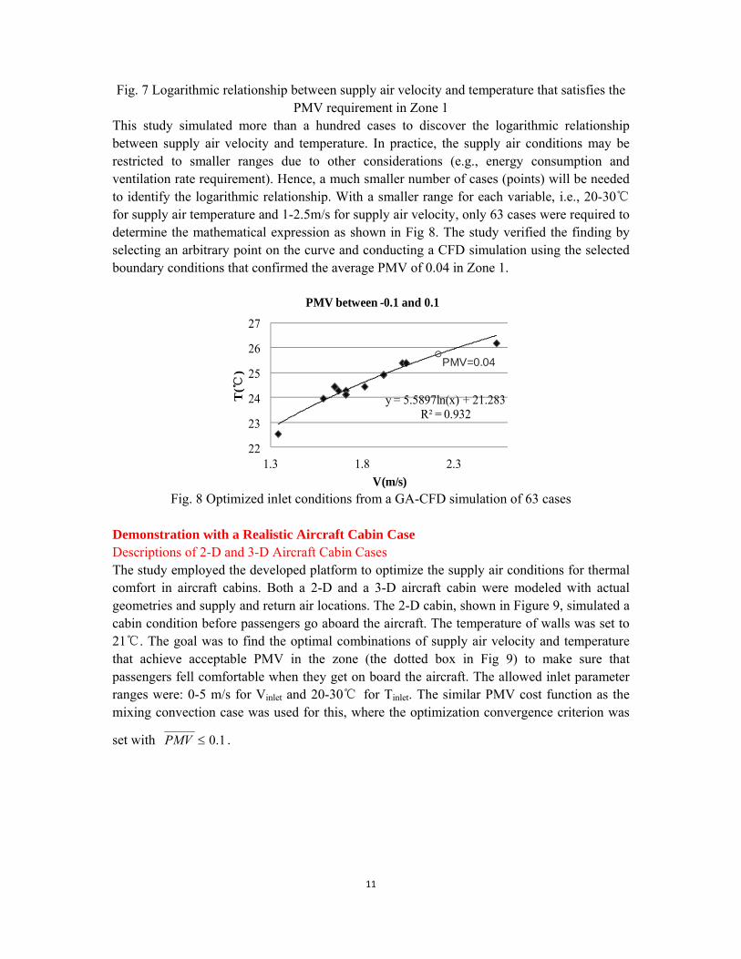
This study simulated more than a hundred cases to discover the logarithmic relationship between supply air velocity and temperature. In practice, the supply air conditions may be restricted to smaller ranges due to other considerations (e.g., energy consumption and ventilation rate requirement). Hence, a much smaller number of cases (points) will be needed to identify the logarithmic relationship. With a smaller range for each variable, i.e., 20-30℃ for supply air temperature and 1-2.5m/s for supply air velocity, only 63 cases were required to determine the mathematical expression as shown in Fig 8. The study verified the finding by selecting an arbitrary point on the curve and conducting a CFD simulation using the selected boundary conditions that confirmed the average PMV of 0.04 in Zone 1.

y = 5.5897ln(x) + 21.283R² = 0.932

22

23

24

25

26

27

1.3 1.8 2.3

T(℃

)

V(m/s)

PMV between -0.1 and 0.1

PMV=0.04

Fig. 8 Optimized inlet conditions from a GA-CFD simulation of 63 cases

Demonstration with a Realistic Aircraft Cabin Case Descriptions of 2-D and 3-D Aircraft Cabin Cases The study employed the developed platform to optimize the supply air conditions for thermal comfort in aircraft cabins. Both a 2-D and a 3-D aircraft cabin were modeled with actual geometries and supply and return air locations. The 2-D cabin, shown in Figure 9, simulated a cabin condition before passengers go aboard the aircraft. The temperature of walls was set to 21℃. The goal was to find the optimal combinations of supply air velocity and temperature that achieve acceptable PMV in the zone (the dotted box in Fig 9) to make sure that passengers fell comfortable when they get on board the aircraft. The allowed inlet parameter ranges were: 0-5 m/s for Vinlet and 20-30℃ for Tinlet. The similar PMV cost function as the mixing convection case was used for this, where the optimization convergence criterion was

set with 0.1PMV .

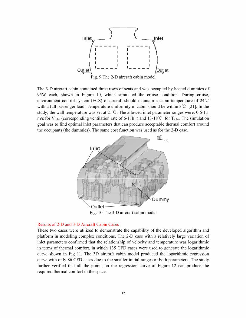
12  

Inlet Inlet

Outlet Outlet 

Fig. 9 The 2-D aircraft cabin model The 3-D aircraft cabin contained three rows of seats and was occupied by heated dummies of 95W each, shown in Figure 10, which simulated the cruise condition. During cruise, environment control system (ECS) of aircraft should maintain a cabin temperature of 24℃ with a full passenger load. Temperature uniformity in cabin should be within 3℃ [21]. In the study, the wall temperature was set at 21℃. The allowed inlet parameter ranges were: 0.6-1.1 m/s for Vinlet (corresponding ventilation rate of 6-11h-1) and 13-18℃ for Tinlet. The simulation goal was to find optimal inlet parameters that can produce acceptable thermal comfort around the occupants (the dummies). The same cost function was used as for the 2-D case.

Inlet

Outlet

Dummy

 

Fig. 10 The 3-D aircraft cabin model  

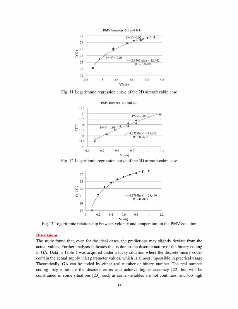
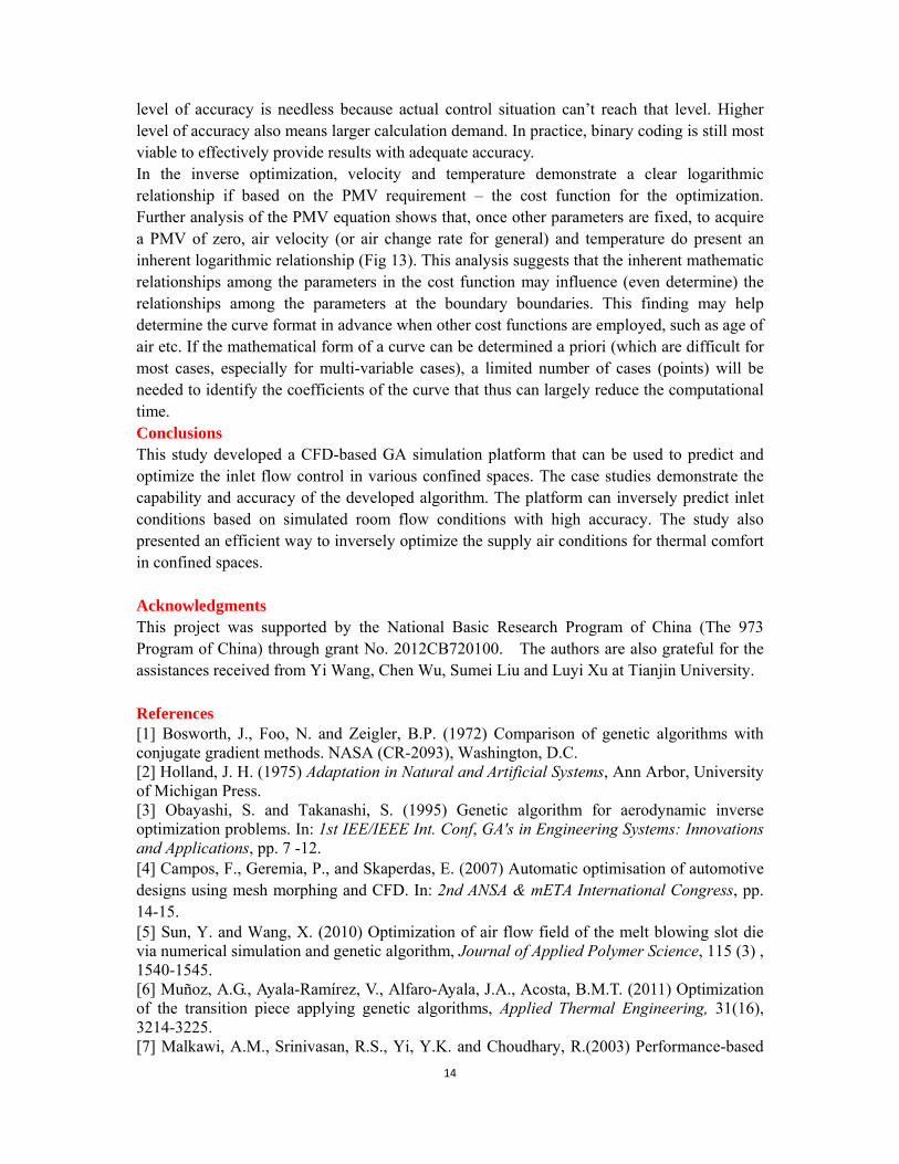
Results of 2-D and 3-D Aircraft Cabin Cases These two cases were utilized to demonstrate the capability of the developed algorithm and platform in modeling complex conditions. The 2-D case with a relatively large variation of inlet parameters confirmed that the relationship of velocity and temperature was logarithmic in terms of thermal comfort, in which 135 CFD cases were used to generate the logarithmic curve shown in Fig 11. The 3D aircraft cabin model produced the logarithmic regression curve with only 86 CFD cases due to the smaller initial ranges of both parameters. The study further verified that all the points on the regression curve of Figure 12 can produce the required thermal comfort in the space.

13  

y = 2.8465ln(x) + 22.443R² = 0.9909

21

22

23

24

25

26

27

0.5 1.5 2.5 3.5 4.5 5.5T

(℃)

V(m/s)

PMV between -0.1 and 0.1

PMV= -0.01

PMV= 0.02

Fig. 11 Logarithmic regression curve of the 2D aircraft cabin case

y = 4.6524ln(x) + 16.613R² = 0.9691

14

14.5

15

15.5

16

16.5

17

17.5

0.6 0.7 0.8 0.9 1 1.1

T(℃

)

V(m/s)

PMV between -0.1 and 0.1

PMV=-0.01

PMV=0.03

 

Fig. 12 Logarithmic regression curve of the 3D aircraft cabin case

y = 4.5797ln(x) + 28.446R² = 0.9823

17

19

21

23

25

27

0 0.2 0.4 0.6 0.8 1 1.2

Ta（

℃）

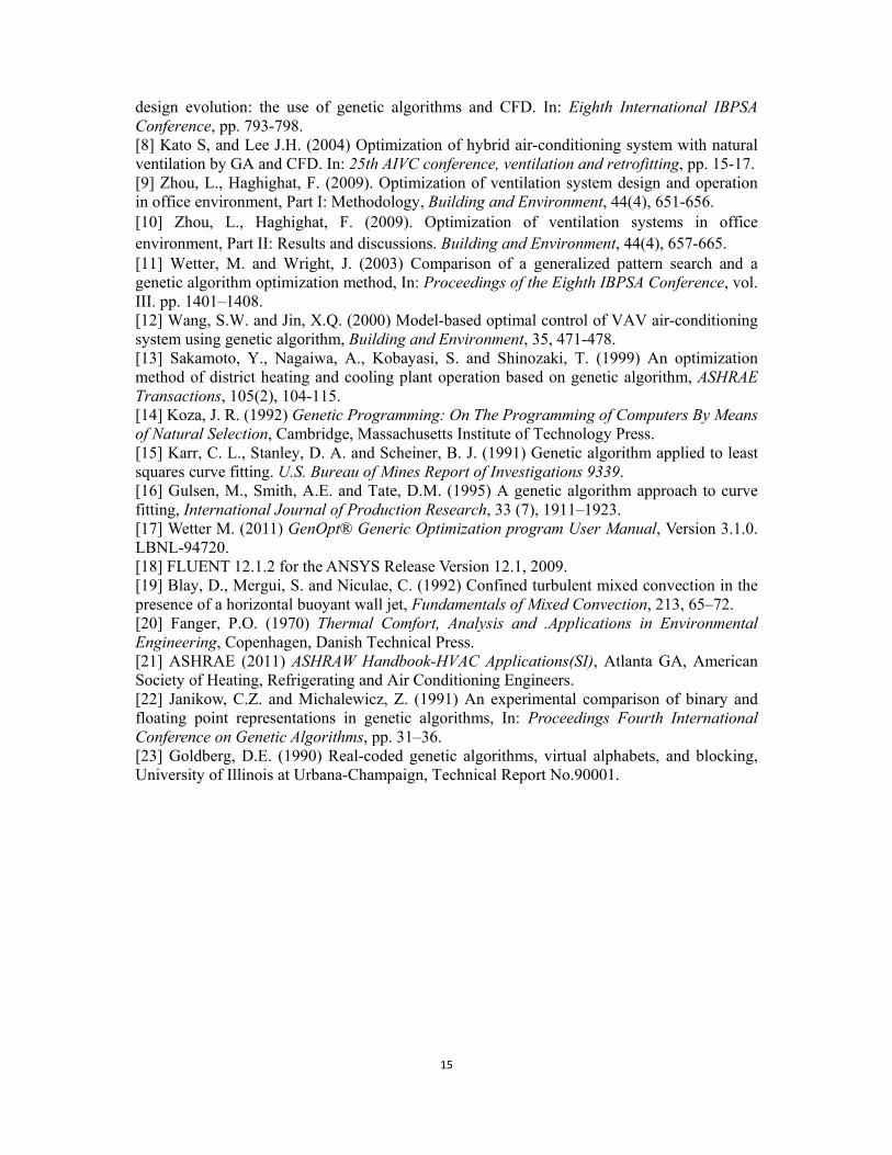
V(m/s)  Fig.13 Logarithmic relationship between velocity and temperature in the PMV equation

Discussions The study found that, even for the ideal cases, the predictions may slightly deviate from the actual values. Further analysis indicates this is due to the discrete nature of the binary coding in GA. Data in Table 1 was acquired under a lucky situation where the discrete binary codes contain the actual supply inlet parameter values, which is almost impossible in practical usage. Theoretically, GA can be coded by either real number or binary number. The real number coding may eliminate the discrete errors and achieve higher accuracy [22] but will be constrained in some situations [23], such as some variables are not continues, and too high

14  

level of accuracy is needless because actual control situation can’t reach that level. Higher level of accuracy also means larger calculation demand. In practice, binary coding is still most viable to effectively provide results with adequate accuracy. In the inverse optimization, velocity and temperature demonstrate a clear logarithmic relationship if based on the PMV requirement – the cost function for the optimization. Further analysis of the PMV equation shows that, once other parameters are fixed, to acquire a PMV of zero, air velocity (or air change rate for general) and temperature do present an inherent logarithmic relationship (Fig 13). This analysis suggests that the inherent mathematic relationships among the parameters in the cost function may influence (even determine) the relationships among the parameters at the boundary boundaries. This finding may help determine the curve format in advance when other cost functions are employed, such as age of air etc. If the mathematical form of a curve can be determined a priori (which are difficult for most cases, especially for multi-variable cases), a limited number of cases (points) will be needed to identify the coefficients of the curve that thus can largely reduce the computational time. Conclusions This study developed a CFD-based GA simulation platform that can be used to predict and optimize the inlet flow control in various confined spaces. The case studies demonstrate the capability and accuracy of the developed algorithm. The platform can inversely predict inlet conditions based on simulated room flow conditions with high accuracy. The study also presented an efficient way to inversely optimize the supply air conditions for thermal comfort in confined spaces. Acknowledgments This project was supported by the National Basic Research Program of China (The 973 Program of China) through grant No. 2012CB720100. The authors are also grateful for the assistances received from Yi Wang, Chen Wu, Sumei Liu and Luyi Xu at Tianjin University. References [1] Bosworth, J., Foo, N. and Zeigler, B.P. (1972) Comparison of genetic algorithms with conjugate gradient methods. NASA (CR-2093), Washington, D.C. [2] Holland, J. H. (1975) Adaptation in Natural and Artificial Systems, Ann Arbor, University of Michigan Press. [3] Obayashi, S. and Takanashi, S. (1995) Genetic algorithm for aerodynamic inverse optimization problems. In: 1st IEE/IEEE Int. Conf, GA's in Engineering Systems: Innovations and Applications, pp. 7 -12. [4] Campos, F., Geremia, P., and Skaperdas, E. (2007) Automatic optimisation of automotive designs using mesh morphing and CFD. In: 2nd ANSA & mETA International Congress, pp. 14-15. [5] Sun, Y. and Wang, X. (2010) Optimization of air flow field of the melt blowing slot die via numerical simulation and genetic algorithm, Journal of Applied Polymer Science, 115 (3) , 1540-1545. [6] Muñoz, A.G., Ayala-Ramírez, V., Alfaro-Ayala, J.A., Acosta, B.M.T. (2011) Optimization of the transition piece applying genetic algorithms, Applied Thermal Engineering, 31(16), 3214-3225. [7] Malkawi, A.M., Srinivasan, R.S., Yi, Y.K. and Choudhary, R.(2003) Performance-based

15  

design evolution: the use of genetic algorithms and CFD. In: Eighth International IBPSA Conference, pp. 793-798. [8] Kato S, and Lee J.H. (2004) Optimization of hybrid air-conditioning system with natural ventilation by GA and CFD. In: 25th AIVC conference, ventilation and retrofitting, pp. 15-17. [9] Zhou, L., Haghighat, F. (2009). Optimization of ventilation system design and operation in office environment, Part I: Methodology, Building and Environment, 44(4), 651-656. [10] Zhou, L., Haghighat, F. (2009). Optimization of ventilation systems in office environment, Part II: Results and discussions. Building and Environment, 44(4), 657-665. [11] Wetter, M. and Wright, J. (2003) Comparison of a generalized pattern search and a genetic algorithm optimization method, In: Proceedings of the Eighth IBPSA Conference, vol. III. pp. 1401–1408. [12] Wang, S.W. and Jin, X.Q. (2000) Model-based optimal control of VAV air-conditioning system using genetic algorithm, Building and Environment, 35, 471-478. [13] Sakamoto, Y., Nagaiwa, A., Kobayasi, S. and Shinozaki, T. (1999) An optimization method of district heating and cooling plant operation based on genetic algorithm, ASHRAE Transactions, 105(2), 104-115. [14] Koza, J. R. (1992) Genetic Programming: On The Programming of Computers By Means of Natural Selection, Cambridge, Massachusetts Institute of Technology Press. [15] Karr, C. L., Stanley, D. A. and Scheiner, B. J. (1991) Genetic algorithm applied to least squares curve fitting. U.S. Bureau of Mines Report of Investigations 9339. [16] Gulsen, M., Smith, A.E. and Tate, D.M. (1995) A genetic algorithm approach to curve fitting, International Journal of Production Research, 33 (7), 1911–1923. [17] Wetter M. (2011) GenOpt® Generic Optimization program User Manual, Version 3.1.0. LBNL-94720. [18] FLUENT 12.1.2 for the ANSYS Release Version 12.1, 2009. [19] Blay, D., Mergui, S. and Niculae, C. (1992) Confined turbulent mixed convection in the presence of a horizontal buoyant wall jet, Fundamentals of Mixed Convection, 213, 65–72. [20] Fanger, P.O. (1970) Thermal Comfort, Analysis and .Applications in Environmental Engineering, Copenhagen, Danish Technical Press. [21] ASHRAE (2011) ASHRAW Handbook-HVAC Applications(SI), Atlanta GA, American Society of Heating, Refrigerating and Air Conditioning Engineers. [22] Janikow, C.Z. and Michalewicz, Z. (1991) An experimental comparison of binary and floating point representations in genetic algorithms, In: Proceedings Fourth International Conference on Genetic Algorithms, pp. 31–36. [23] Goldberg, D.E. (1990) Real-coded genetic algorithms, virtual alphabets, and blocking, University of Illinois at Urbana-Champaign, Technical Report No.90001.