inverse problems and optimization - ntnu · tma 4180 optimeringsteori 2010 inverse problems and...

TMA 4180 Optimeringsteori 2010

INVERSE PROBLEMS AND OPTIMIZATION

TMA 4180 Optimeringsteori

Harald E. Krogstad, IMF, Spring. 2010


CONTENTS

• Inverse problems• Some famous problems• Examples• Techniques


Jeopardy - The everyday Inverse problem:

“When did Norway and Sweden split up from the union?”

“When was my grandmother born?”

“When did Robert Koch get the Nobel Price in Medicine?”

“When did Einstein publish his Theory of Relativity ?”

“It was in 1905”


• The information is incomplete and non-conclusive

• Different input leads to the same result

• The ”most probable” input depends on circumstances

direct problem: given the question, find the answer

inverse problem: given the answer, find the question


Well-posed problems (Hadamard, 1923): • a solution always exists • there is only one solution • a small change in the problem leads to a small change

in the solution

INVERSE PROBLEMS ARE (ALMOST) ALWAYS ILL-POSED!

Ill-posed problems:• a solution may not exist • there may be more than one solution • a small change in the problem leads to a

big change in the solution


SOME FAMOUS INVERSE PROBLEMS

• Marc Kac (1966): "Can you hear the shape of a drum?"

• Seismic Inversion

• Computer Tomography

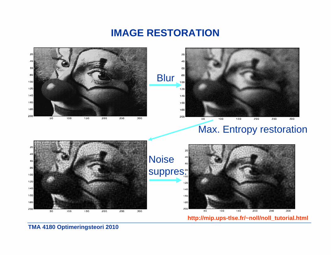
• Image Restoration

TMA 4180 Optimeringsteori 2010http://www.ams.org/new-in-math/hap-drum/hap-drum.html

NO, you can’t hear the shape of a drum, but you can hear

• the area, • the length of the boundary,• and the number of holes!

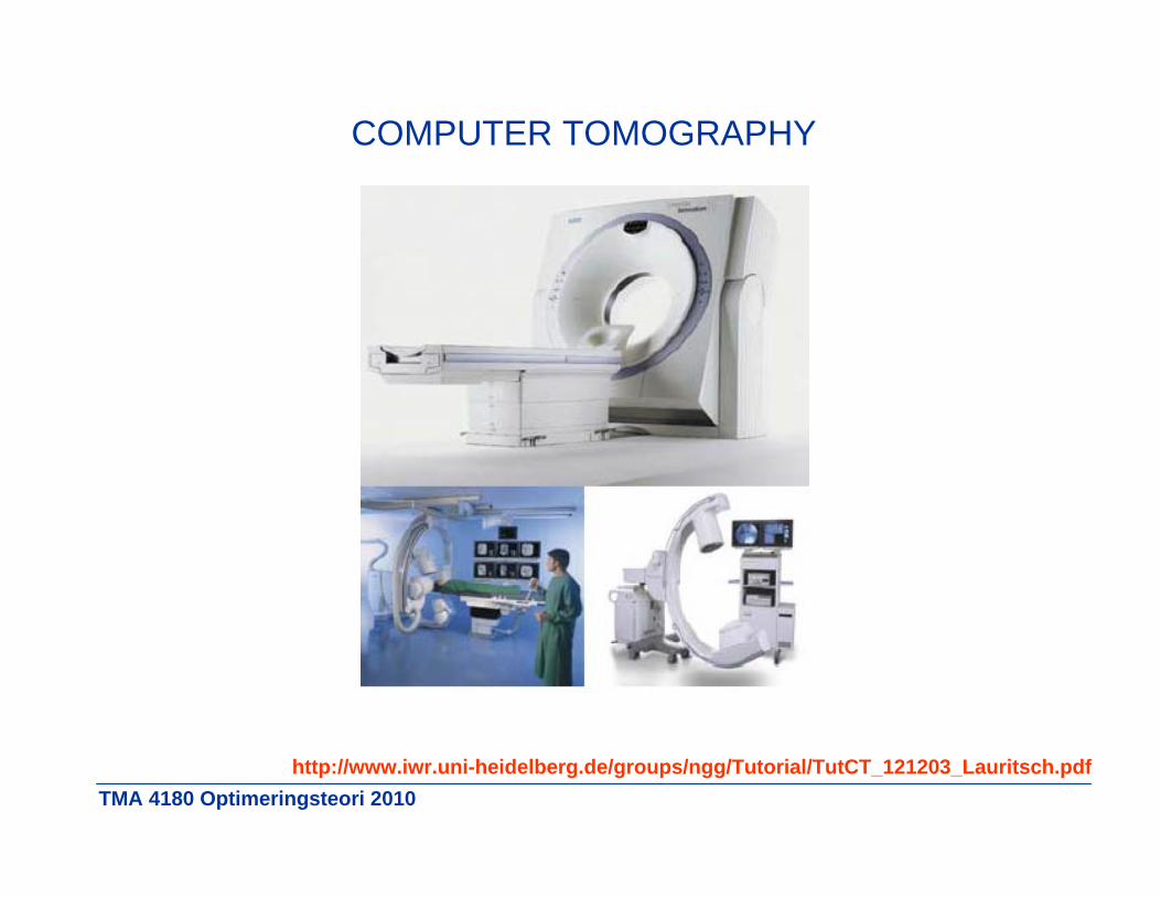
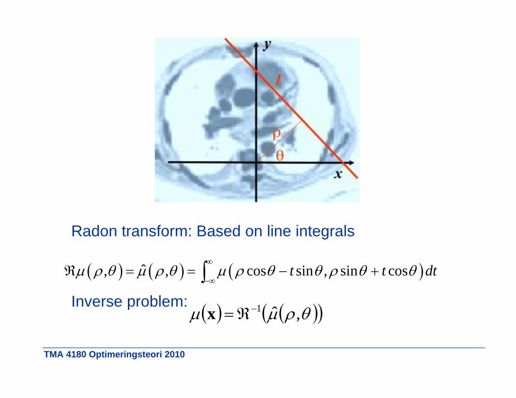
TMA 4180 Optimeringsteori 2010http://www.iwr.uni-heidelberg.de/groups/ngg/Tutorial/TutCT_121203_Lauritsch.pdf

COMPUTER TOMOGRAPHY


jlinej dlII xexp0


Radon transform: Based on line integrals

Inverse problem:

ˆ, , cos sin , sin cost t dt

,ˆ1x


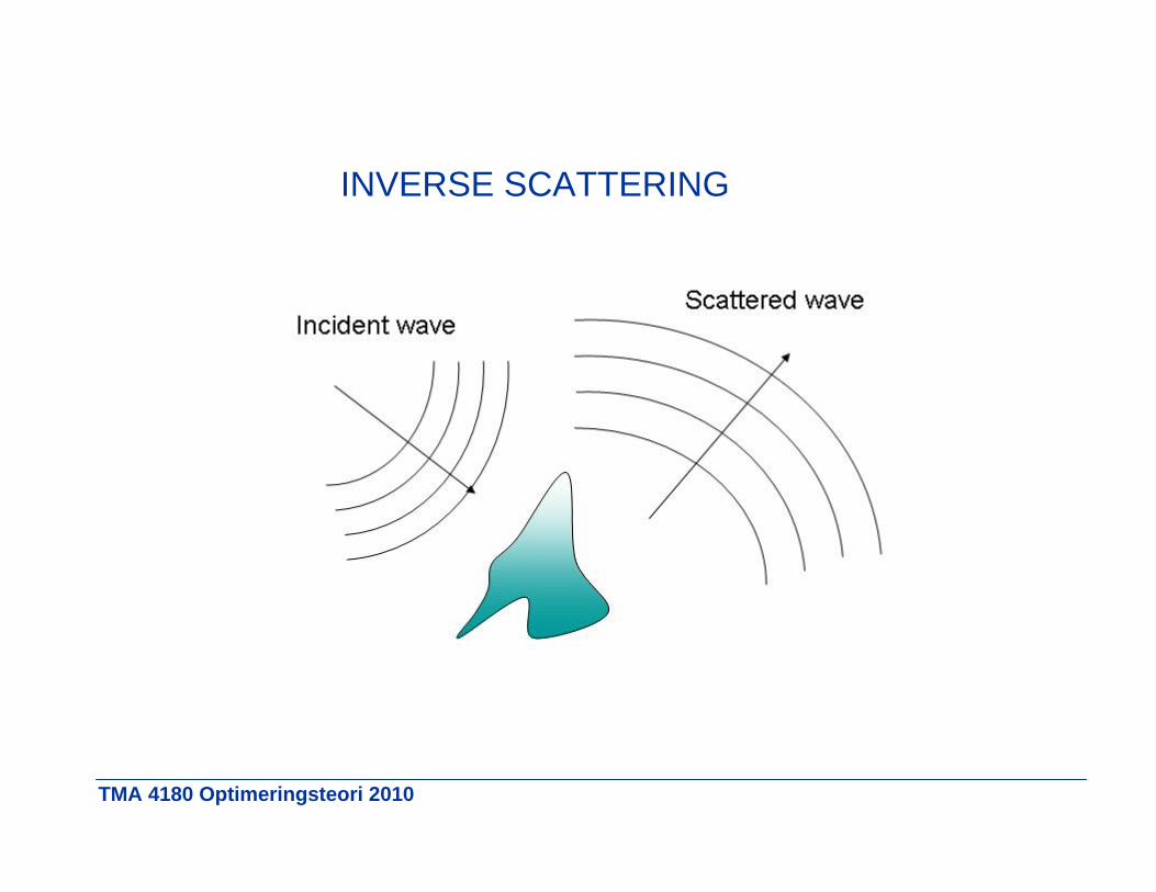
INVERSE SCATTERING

TMA 4180 Optimeringsteori 2010http://www.mgnet.org/~douglas/Classes/cs521-s00/asdf/asdf.ppt

Seismic inversion


Resistivity map for a major North Sea field, 3D EM method. (Data courtesy of EMGS and Statoil Hydro)

GasOil

(Houston Geological Society)


Compute sea floor motion from seismic recordings:UpliftSlip

(Bjørn Gjevik, UiO. Published by Caltech)

(The December 26, 2004, Sumatran Tsunami)


MEDICAL ULTRASOUND

(Trond Varslot)


Blur

Max. Entropy restoration

Noisesuppres.

IMAGE RESTORATION

http://mip.ups-tlse.fr/~noll/noll_tutorial.html


A: Original HST photo. B: Enlarged section. C: Ground telescope image. D: Digitally enhanced image. ©ESA


LINEAR, NOISE-FREE PROBLEMS

nxR A mb Ax RInput Filter Observation

'A U V Singular value decomposition:

*

1

''

rank Aj

jj j

u bx A b V U b v

Regularization: Truncated SVD (TSVD):

(unstable)

1

'KjK

jj j

u bx v


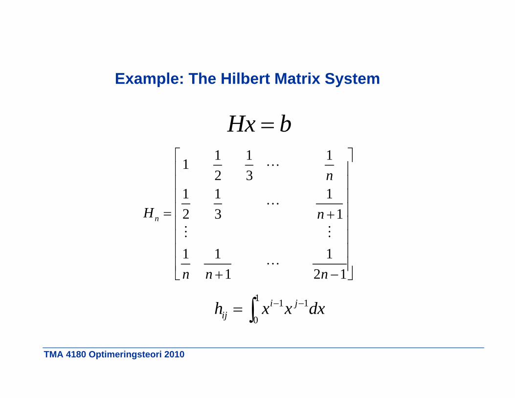
1 1 112 3

1 1 12 3 1

1 1 11 2 1

n

n

H n

n n n

Hx b

1 1 1

0

i jijh x x dx

Example: The Hilbert Matrix System


0 10 2010-20

10-10

100

1010 Singular values

0 10 20-200

-100

0

100

200

300Exact and direct solutions

0 10 201

1.5

2

2.5

3

3.55 terms

0 10 201

1.5

2

2.5

3

3.510 terms

0 10 20-20

-10

0

10

2015 terms

0 10 20

10-1

100

101ut

i b/ i

(cond. Number = 1.5x1018)

Picard-plot


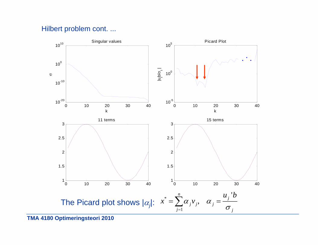
Hilbert problem cont. ...

0 10 20 30 4010-20

10-10

100

1010 Singular values

k

0 10 20 30 4010-5

100

105 Picard Plot

k

|uib/

i |

0 10 20 30 401

1.5

2

2.5

311 terms

0 10 20 30 401

1.5

2

2.5

315 terms

The Picard plot shows |j|:*

1

',

nj

j j jj j

u bx v



WARNING: A small residual does not mean a good solutionfor ill-conditioned problems:

0 10 20 30 4010-15

10-10

10-5

100

105 Res iual

k

||Ax-

b||

0 10 20 30 40101

102

103

104

105 Norm of x

k

||x||


0 0.2 0.4 0.6 0.8 1 1.20

0.5

1

1.5

k/k0

Tape

r

A smooth cut-off: The cosine taper



TIKHONOV REGULARIZATION

• We expect that X is close to :

2 2*0arg min XX T X Y X X

0X

• We expect that X is smooth:

2 2* arg min ( )XX T X Y L X

(The L operator punishes irregularities)

Error term Regularization term

Weight


Hodrick-Prescott Filter

1800 1820 1840 1860 1880 1900 1920 1940 1960 1980 2000

2

4

6

8

10

Tem

pera

ture

, o C

Year

Yearly mean temperatures and trend curve, Blindern, Oslo

1800 1820 1840 1860 1880 1900 1920 1940 1960 1980 2000

2

4

6

8

10

Tem

pera

ture

, o C

Year

Trend

1800 1820 1840 1860 1880 1900 1920 1940 1960 1980 2000-4

-2

0

2

4

Tem

pera

ture

, o C

Year

Residuals


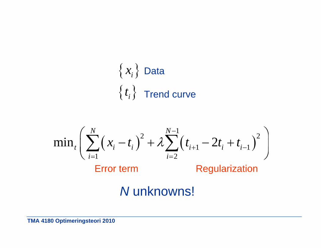
Data

Trend curve

i

i

x

t

1

2 21 1

1 2

min 2N N

t i i i i ii i

x t t t t

N unknowns!

Error term Regularization


1800 1820 1840 1860 1880 1900 1920 1940 1960 1980 2000

2

4

6

8

10

Tem

pera

ture

, o C

B lindern , Oslo, =100

1800 1820 1840 1860 1880 1900 1920 1940 1960 1980 2000

2

4

6

8

10

Tem

pera

ture

, o C

=1500

1800 1820 1840 1860 1880 1900 1920 1940 1960 1980 2000

2

4

6

8

10

Tem

pera

ture

, o C

Year

=100000


THE KEY PROBLEM

• How to select the best/most probable/optimal solution

• How to dampen ”ill-conditionness”(regularize - but not exaggerate!)

2 2*0arg min XX T X Y X X

small: solution unstable (ill-conditioned problem)

large: (even if our ”knowledge” is false!) *0X X

Example: Tikhonov regularization

0X


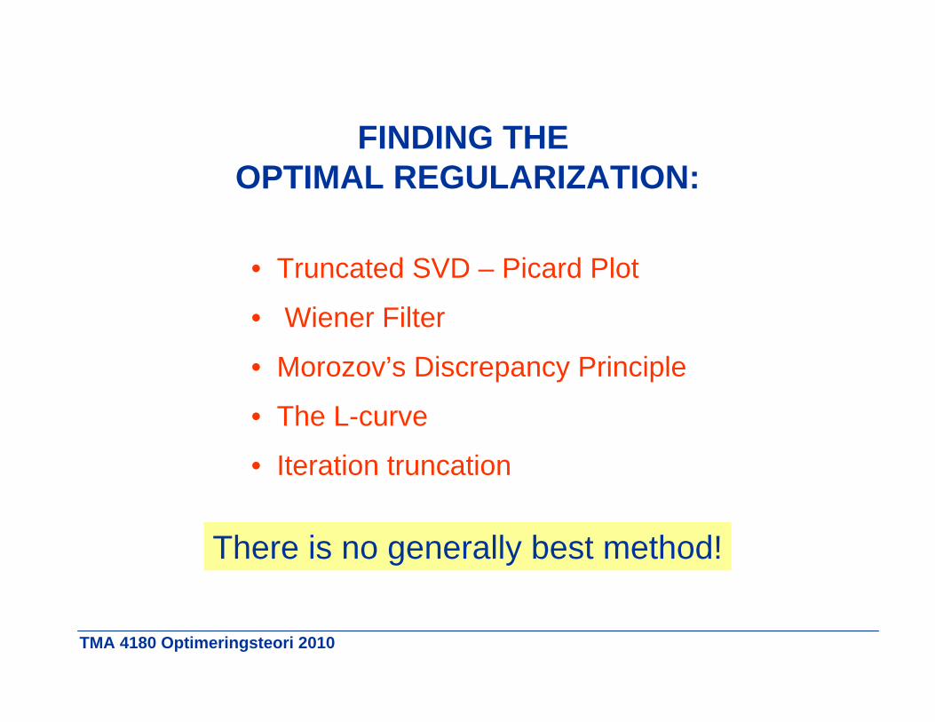
FINDING THE OPTIMAL REGULARIZATION:

• Truncated SVD – Picard Plot

• Wiener Filter

• Morozov’s Discrepancy Principle

• The L-curve

• Iteration truncation

There is no generally best method!


FREDHOLM INTEGRAL EQUATIONS

1

0,y t K t x d

K(t,) is called the kernel

Discretized Fredholm Integral Equationsare generally ill-conditioned


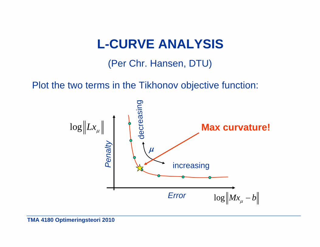
L-CURVE ANALYSIS(Per Chr. Hansen, DTU)

Plot the two terms in the Tikhonov objective function:

log Mx b

log Lx

increasing

Error

Pen

alty

decr

easi

ngMax curvature!


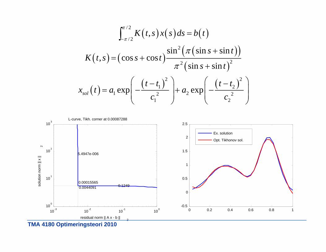
/ 2

/ 2

2

22

2 21 2

1 22 21 2

,

sin sin sin, cos cos

sin sin

exp expsol

K t s x s ds b t

s tK t s s t

s t

t t t tx t a a

c c

10-3

10-2

10-1

100

100

101

102

103

0.12490.00440910.00015565

5.4947e-006

residual norm || A x - b ||2

solu

tion

norm

|| x

||2

L-curve, Tikh. corner at 0.00087288

0 0.2 0.4 0.6 0.8 1-0.5

0

0.5

1

1.5

2

2.5

Ex. solution

Opt. Tikhonov sol.


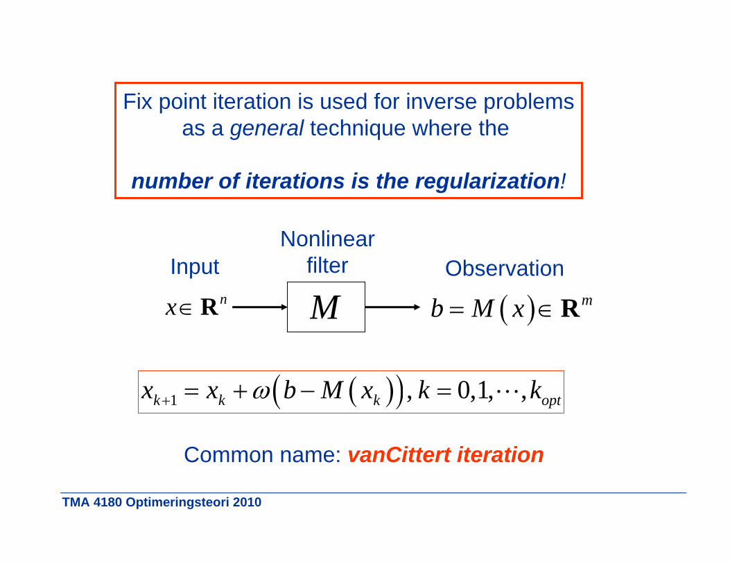
ITERATIVE METHODSThe basic iterative method for a linear equation

is

(“fix-point iteration”)

is called a relaxation parameter.

Convergence if is chosen so that

, 0,Ax b A

1 , 0,1,k k kx x b Ax k

1I A


Fix point iteration is used for inverse problemsas a general technique where the

number of iterations is the regularization!

nxR M mb M x RInput

Nonlinearfilter Observation

Common name: vanCittert iteration

1 , 0,1, ,k k k optx x b M x k k


DE-CONVOLUTION OF SPECTRAL DATA

• Astronomy• Mass spectrography• Optics• Nuclear Magnetic Resonance

Measurement should consist of narrow “spectral lines”,but the instrument “blurs” the lines:

“De-blurring” is needed!


1 max 0, , 0,1, ,k k blur k optx x b g x k k

0 0.1 0.2 0.3 0.4 0.5 0.6 0.7 0.8 0.9 10

0.5

1

Spec

trum

Measurement

0 0.1 0.2 0.3 0.4 0.5 0.6 0.7 0.8 0.9 10

0.5

1

Spec

trum

De-convoluted measurement

0 0.1 0.2 0.3 0.4 0.5 0.6 0.7 0.8 0.9 10

0.5

1

Frequency

Spec

trum

"Ideal" measurement

2000 iterations!


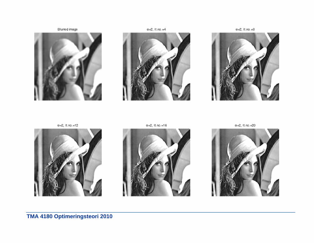
A very common situation in image processing:

2( ) * ( ) ( )PS PSBI f I f I d Rx x x y y y

I : ImageBI : Blurred imagefPS : Point Spread Function

BI I : ”Deconvolution”

1 max 0, * , 1,2, ,k k PS k stopI I BI f I k k

(NB: Should have some idea about fPS !


vanCittert/Landweber iteration is simple and fast!


MORE INFORMATION:

Google: ”Inverse Problems” 1 850 000 hits!

Bibsys: ”Inverse Problems” 155 items

Wikipedia:http://en.wikipedia.org/wiki/Inverse_problem(incomplete)

Per Chr. Hansen’s home page:http://www.imm.dtu.dk/~pch/ (recommended!)

Albert Tarantola's home page:http://www.ipgp.fr/~tarantola/ (amusing!)

inverse problems and optimization - ntnu · tma 4180 optimeringsteori 2010 inverse problems and...

Documents