inversion for refractivity parameters from radar sea...

$: Inversion for refractivity parameters from radar sea clutternoiselab.ucsd.edu/papers/Gerstoft2003rfc.pdf · Inversion for refractivity parameters from radar sea clutter Peter Gerstoft,1$
Inversion for refractivity parameters from radar sea clutter

Peter Gerstoft,1 L. Ted Rogers,2 Jeffrey L. Krolik,3 and William S. Hodgkiss1

Received 5 March 2002; revised 31 May 2002; accepted 10 July 2002; published 4 April 2003.

[1] This paper describes estimation of low-altitude atmospheric refractivity from radar seaclutter observations. The vertical structure of the refractive environment is modeled usingfive parameters, and the horizontal structure is modeled using six parameters. Therefractivity model is implemented with and without an a priori constraint on the ductstrength, as might be derived from soundings or numerical weather-prediction models. Anelectromagnetic propagation model maps the refractivity structure into a replica field.Replica fields are compared to the observed clutter using a squared-error objectivefunction. A global search for the 11 environmental parameters is performed using geneticalgorithms. The inversion algorithm is implemented on S-band radar sea-clutter data fromWallops Island, Virginia. Reference data are from range-dependent refractivity profilesobtained with a helicopter. The inversion is assessed (1) by comparing the propagationpredicted from the radar-inferred refractivity profiles and from the helicopter profiles, (2)by comparing the refractivity parameters from the helicopter soundings to those estimated,and (3) by examining the fit between observed clutter and optimal replica field. Thistechnique could provide near-real-time estimation of ducting effects. In practicalimplementations it is unlikely that range-dependent soundings would be available. Asingle sounding is used for evaluating the radar-inferred environmental parameters. Whenthe unconstrained environmental model is used, the ‘‘refractivity-from-clutter,’’ thepropagation loss generated and the loss from this single sounding, is close within the duct;however, above the duct they differ. Use of the constraint on the duct strength leads toa better match also above the duct. INDEX TERMS: 3360 Meteorology and Atmospheric Dynamics:

Remote sensing; 6904 Radio Science: Atmospheric propagation; 6969 Radio Science: Remote sensing;

6982 Radio Science: Tomography and imaging; KEYWORDS: atmospheric refractivity estimation, radar

clutter, genetic algorithms, radar cross section

Citation: Gerstoft, P., L. T. Rogers, J. L. Krolik, and W. S. Hodgkiss, Inversion for refractivity parameters from radar sea

clutter, Radio Sci., 38(3), 8053, doi:10.1029/2002RS002640, 2003.

1. Introduction

[2] Two common refractivity structures that signifi-cantly affect the performance of shipboard radars areevaporation ducts and surface-based ducts (see Figure 1).When a duct is present the low altitude propagation losswill usually be much less than for a standard atmosphere,

and thus increasing the range at which low-altitudetargets can be detected.[3] Surface-based ducts appear about 15% of the time

worldwide, 25% of the time off Southern CaliforniaCoast, and 50% of the time in the Persian Gulf [Patter-son, 1992]. While surface-based ducts are less commonthan evaporation ducts, their effects frequently are moredramatic. They often manifest themselves in a radar’splan position indicator (PPI) as clutter rings, see Figure 2(the SPANDAR radar is described in section 2), and theycan result in significant height errors for 3-D radar as thelowest elevation scans become trapped on the surfaceinstead of refracting upward as would be expected for astandard atmosphere. Many efforts in remote sensing andnumerical weather prediction have been directed atbetter estimation of the refractivity structure in the lowest1000 m above the sea surface [see Richter, 1995; Rogers,1997]. Alternatives for estimating the refractivity struc-

RADIO SCIENCE, VOL. 38, NO. 3, 8053, doi:10.1029/2002RS002640, 2003

1Marine Physical Laboratory, University of California, San Diego,La Jolla, California, USA.

2Atmospheric Propagation Branch, Space and Naval WarfareSystems Command Systems Center, San Diego, California, USA.

3Department of Electrical and Computer Engineering, DukeUniversity, Durham, North Carolina, USA.

Copyright 2003 by the American Geophysical Union.

0048-6604/03/2002RS002640$11.00

MAR 18 - 1

ture that is not associated with the surface layer are insitu sampling via radiosondes or rocketsondes [Rowlandet al., 1996], or through numerical weather predictionmodels [see Haack and Burk, 2001].[4] Because the effects of surface-based ducting are

visibly manifested in radar clutter, it might be feasible toextract information about the duct’s refractive structurefrom the clutter. Such a ‘‘refractivity-from-clutter’’ (RFC)capability might provide near-real-time, azimuth-depend-ent information about the ducting conditions, as opposed

to current practice where the characterization is basedonly on the ship-launched in situ instrument, whose time-lateness is from tens of minutes to several hours. Fur-thermore, RFC might require no emissions beyond thoseinherent in the operation of the ship’s radar, nor wouldRFC require additional deck-mounted equipment; theseare critical considerations.[5] Inferring refractivity parameters from observations

of radar clutter is an inverse problem. The Bayesianframework for solving for solving such problems is laid

Figure 1. Modified refractivity M versus height. (a) Evaporation duct (typical height 0–30 m);(b) surface-based duct (typical height 30–1000 m); (c) elevated duct. The modified refractivity isthe refractivity multiplied with 106 and corrected for the curvature of Earth.

Figure 2. Reflectivity map (dBZ) from SPANDAR corresponding to Wallops run 12 (time13:00EST, see also section 2). The elevation angle is 0� and horizontal and vertical range are inkilometers.

MAR 18 - 2 GERSTOFT ET AL.: REFRACTIVITY FROM CLUTTER

out by Tarantola [1987]. Within the Bayesian frame-work, the general steps involved in RFC for surface-based ducts are as follows:[6] 1. The input data is a vector of received clutter

power values Pcobs at discrete ranges r1, r2, . . . rN.

[7] 2. An environmental model Henv maps an environ-mental parameter vector m into M, a vector or matrix ofvalues of modified refractivityM over the discrete rangesand heights of interest.[8] 3. A combined electromagnetic (EM) propagation

model (we use TPEM [Barrios, 1994]) and radarmodel Hprop maps M into a replica field Pc(m) =Hprop(Henv(m)).[9] 4. An objective function f calculates the fit of

Pc(m) to Pcobs.

[10] 5. A global optimization procedure is used searchover all m to find the optimal value bm of the f (Pc

obs,Pc(m)).[11] 6. An assessment is made of the quality of the

solution by examining forward model solutions orparameter error estimates/distributions [see, e.g., Gerstoftand Mecklenbrauker, 1998]. This is important as a globalsolution always will provide an estimate, and, for exam-ple, it could indicate that a wrong environmental modelis used. For convenience, we refer to this as a ‘‘globalparameter’’ algorithm since each new combination of theelements of m requires a new run of the forward model.[12] The inference of refractivity parameters associated

with surface-based ducts was first posed by Krolik andTabrikian [1998] as a maximum a posteriori (MAP)estimation problem. In that initial work, the environ-mental parameter vector m had only three elements: twoto describe the vertical structure of refractivity and one todescribe the range dependency of the environment. Thealgorithm worked well in some instances; however, oftenthe optimal replica field did not match the observed data.This phenomenon could be attribute to the horizontalvariability of the-sea clutter radar cross section s�. It ismore likely, however, that the dominant problem washaving too simple a model for the refractive environ-ment, one that could not account for variations thatresulted in horizontal shifting of features. Note, however,that while the horizontal variability of s� probably is notthe cause of poor fits, it can have unwanted effects oninversion results and will be examined in section 5.3.[13] The need for greater fidelity in modeling the

refractive environment is being addressed by two groupsusing different methods. Krolik and coworkers are pur-suing the development of a marching algorithm wherethe parameters describing the refractivity are updated ateach range step of the parabolic equation and theenvironmental parameters are assumed to vary as aMarkov process with respect to range. The latest resultsusing the marching algorithm [Anderson et al., 2001] arecomparable to the results that presented here.

[14] This paper focuses on using a global-parametersapproach with parameterizations of both vertical andhorizontal structure of the refractive environment. This,then, is a multi-parameter optimization problem that issolved using a genetic algorithm search strategy [Ger-stoft, 1994]. How the global parameter approach isrealized reflects the varying degrees of maturity of theindividual components:[15] 1. There is no clearly identified ‘‘best’’ choice for

Henv; the map from m to Pc(m) is always nonlinear asHprop is nonlinear. That precludes the use of tools such asKarhunen-Loeve for identifying principal components.In general, we expect that adding more parameters musually will result in a better match to Pc

obs. But, ifneither Henv nor additional a priori restrictions on mconstrain the solution, then unrealistic values may beestimated. Additionally, adding more parametersincreases the size of the search space. Thus developingHenv is a balance between minimizing the number ofparameters (to minimize the size of the search space) andhaving sufficient parameters so that close fits to Pc

obs canbe obtained, while constraining the solutions such thatM = Henv(m) is restricted to realizations that are con-sistent with refractivity structures observed in nature.[16] 2. The EM propagation models available for

computing Hprop are reasonably mature [Levy, 2000;Dockery, 1998] as is the modeling of the radar system.[17] 3. The modeling of the sea-clutter radar cross

section s� as a function of environmental parametersand its sensitivity to the grazing angle y is somewhat lessmature and is discussed further in section 3.5. We handlethe uncertainty in the modeling of sea clutter by makingour objective function insensitive to the average value ofs�, and thus freeing us of the need for rigorous modelingof the same. At the same time, the first range at which weuse the clutter data is sufficiently distant from the radarto preclude the use of data where large grazing angles arepresent.[18] 4. The objective function f is ideally determined

from knowledge of errors in the forward modeling andthe data. The f we choose is optimal for the case wherethe mismatch between Pc(bm) and Pc

obs is an independent,univariate, Gaussian process. However, it is expected towork well for cases where this is not satisfied.[19] The remainder of this paper reports on the imple-

mentation of the global algorithm and is organized asfollows: Radar observations and in situ validation datafor a ducting event in the vicinity of Wallops Island, VA,on 2 April 1998, are described in section 2. Section 3describes the forward modeling with an emphasis on theenvironmental modeling. The effects of the variability ofthe refractive environment on the clutter returns areillustrated in section 4. The results of implementing theinversion procedure using the above data are given insection 5.

GERSTOFT ET AL.: REFRACTIVITY FROM CLUTTER MAR 18 - 3

[20] The results presented here are for cases where (1)the general nature of the cases considered (a duct createdby the flow of warm, dry, continental air over a relativelycolder ocean) vary little from case to case in comparisonto the variations in ducting structures that would beencountered in a world-wide sampling, and (2) evidencepoints to the sea clutter radar cross section having littlehorizontal variability for the cases considered, whereasgreater variability is likely to be encountered in a world

wide sampling. Testing over a wide range of data cases,as well as making the algorithm robust in the presence ofa range-varying s�, and the use of prior knowledge of s�range dependency are necessary future steps.

2. Radar and Validation Data

[21] Radar and in situ validation data were obtainedduring the Wallops ’98 measurement campaign [Rogerset al., 2000] conducted by the Naval Surface WarfareCenter, Dahlgren Division. The data presented here arefrom the surface-based ducting event that occurred on 2April 1998. Radar data were obtained using the SpaceRange Radar (SPANDAR) [Stahl and Crippen, 1994].[22] The SPANDAR was originally designed as a

tracking radar. It is equipped with (nominal) 4 MWand 1 MW transmitters and an 18.29-m parabolicantenna. Table 1 shows the radar’s parameters as con-figured for the data taken here. Pulse widths (2 ms) on theradar correspond to range-bin widths of 600 m. With 446range bins available, this provides maximum range of

Table 1. Space Range Radar (SPANDAR) Parameters for 2

April 1998 Observations

Parameter Measurement

Frequency, GHz 2.84Power, dBm 91.40Beamwidth, deg 0.39Antenna gain, dB 52.80Height, m. MSL 30.78Polarization VVRange bin width, m 600

Figure 3. Modified refractivity profiles (M units) sequenced in time. The first row is observedfrom 8:47–10:26 EST (08:47–09:05, 09:07–09:32, 09:33–09:57, and 09:58–10:26), middle12:26–14:15 EST (12:26–12:50, 12:52–13:17, 13:19–13:49, and 13:51–14:14), and bottom16:00–16:52 EST (15:59–16:27 and 16:29–16:52). All refractivity profiles have been normalizedto the same value (330 M units) at sea level.


267 km, when the first range bin is set to 0 km. The radaris equipped with a Sigmet Radar Data System thatprovides reflectivity, velocity, time series, and spectratypes of output. However, for the Wallops’98 experimentSignal-to-noise ratio (S/N) was recorded instead ofreflectivity.[23] A polar plot of S/N (or clutter map) at 0� elevation

from a ducting event is shown in Figure 2. The edgesaround radials 30� and 180–200� are due to the coast-line. The intensifications around ranges 130, 180, and230 km are due to ducting propagation. To mitigate theeffects point targets (including sea spikes), the radar dataused in the inversions are median filtered across range(1.2 km, 3 samples) and azimuth (5�, 9 samples).[24] Meteorological soundings were obtained by an

instrumented helicopter provided by the Johns-HopkinsUniversity Applied Physics Laboratory. The helicopterwould fly in and out on the 150� radial from a point 4 kmdue east of the SPANDAR. During the flights, thehelicopter would fly a saw-tooth up-and-down patternand a single transect lasted about 30 min. Contour plotsof modified refractivity versus range and height areshown in Figure 3. Dark lines superimposed on the plotare the modified refractivity profiles. The duct can beseen in the first 100 m. The figure illustrates the range

and time variability on the day of the experiment. Theearlier profiles show substantial range dependency. Thisindicates that for inversion a range-dependent modelmight be needed.[25] The refractivity profiles then were used to generate

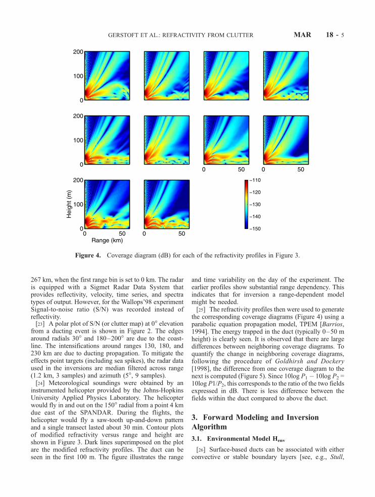
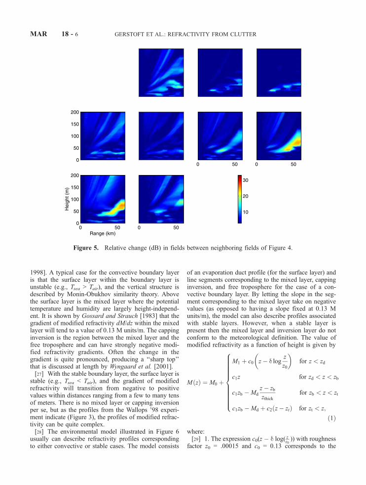
the corresponding coverage diagrams (Figure 4) using aparabolic equation propagation model, TPEM [Barrios,1994]. The energy trapped in the duct (typically 0–50 mheight) is clearly seen. It is observed that there are largedifferences between neighboring coverage diagrams. Toquantify the change in neighboring coverage diagrams,following the procedure of Goldhirsh and Dockery[1998], the difference from one coverage diagram to thenext is computed (Figure 5). Since 10log P1 � 10log P2 =10log P1/P2, this corresponds to the ratio of the two fieldsexpressed in dB. There is less difference between thefields within the duct compared to above the duct.

3. Forward Modeling and Inversion

Algorithm

3.1. Environmental Model Henv

[26] Surface-based ducts can be associated with eitherconvective or stable boundary layers [see, e.g., Stull,

Figure 4. Coverage diagram (dB) for each of the refractivity profiles in Figure 3.


1998]. A typical case for the convective boundary layeris that the surface layer within the boundary layer isunstable (e.g., Tsea > Tair), and the vertical structure isdescribed by Monin-Obukhov similarity theory. Abovethe surface layer is the mixed layer where the potentialtemperature and humidity are largely height-independ-ent. It is shown by Gossard and Strauch [1983] that thegradient of modified refractivity dM/dz within the mixedlayer will tend to a value of 0.13 M units/m. The cappinginversion is the region between the mixed layer and thefree troposphere and can have strongly negative modi-fied refractivity gradients. Often the change in thegradient is quite pronounced, producing a ‘‘sharp top’’that is discussed at length by Wyngaard et al. [2001].[27] With the stable boundary layer, the surface layer is

stable (e.g., Tsea < Tair), and the gradient of modifiedrefractivity will transition from negative to positivevalues within distances ranging from a few to many tensof meters. There is no mixed layer or capping inversionper se, but as the profiles from the Wallops ’98 experi-ment indicate (Figure 3), the profiles of modified refrac-tivity can be quite complex.[28] The environmental model illustrated in Figure 6

usually can describe refractivity profiles correspondingto either convective or stable cases. The model consists

of an evaporation duct profile (for the surface layer) andline segments corresponding to the mixed layer, cappinginversion, and free troposphere for the case of a con-vective boundary layer. By letting the slope in the seg-ment corresponding to the mixed layer take on negativevalues (as opposed to having a slope fixed at 0.13 Munits/m), the model can also describe profiles associatedwith stable layers. However, when a stable layer ispresent then the mixed layer and inversion layer do notconform to the meteorological definition. The value ofmodified refractivity as a function of height is given by

M zð Þ ¼ M0 þ

M1 þ c0 z� d logz

z0

� �for z < zd

c1z for zd < z < zb

c1zb �Md

z� zb

zthickfor zb < z < zt

c1zb �Md þ c2 z� ztð Þ for zt < z;

8>>>>>>>>><>>>>>>>>>:

ð1Þ

where:[29] 1. The expression c0(z � d log( z

z0)) with roughness

factor z0 = .00015 and c0 = 0.13 corresponds to the

Figure 5. Relative change (dB) in fields between neighboring fields of Figure 4.


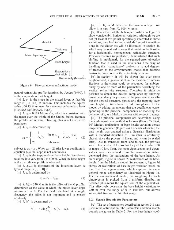
neutral refractivity profile described by Paulus [1990]. dis the evaporation duct height.[30] 2. c1 is the slope in the mixed layer. A feasible

range is [�1, 0.4] M units/m. This includes the typicalvalue of 0.13 M units/m for a convective boundary layer[Gossard and Strauch, 1983].[31] 3. c2 = 0.118 M units/m, which is consistent with

the mean over the whole of the United States. Becausethe profiles are upward refracting, this is not a sensitiveparameter.[32] 4. zd is determined by

zd ¼d

1� c1=c0for 0 <

1

1� c1=c0< 2

2d otherwise

8><>: ; ð2Þ

subject to zd < zb. When zd = 2d (the lower condition inequation (2)) the slope is not continuous.[33] 5. zb is the trapping-layer base height. We choose

to allow it to vary from 0 to 500 m. When the base heightis 0 m, a bilinear profile is obtained.[34] 6. zthick is thickness of the inversion layer. A

typical range is [0, 100] m.[35] 7. zt is determined by

zt ¼ zb þ zthick: ð3Þ

[36] 8. M0 = 330 M units is the offset of the M profile,determined as the value at which the mixed layer slopeintersects z = 0. For the field calculated at a singlefrequency, the offset is not important and is chosenarbitrarily.[37] 9. M1 is determined by

[38] 10. Md is M deficit of the inversion layer. Weallow it to vary from [0, 100] M units.[39] It is clear that the helicopter profiles in Figure 3

show considerably horizontal variation. Although we arenot (at least at this point) specifically interested in thesevariations, they lead to horizontal shifting of intensifica-tions in the clutter (as will be illustrated in section 4),which may be realized in ways that might not be feasiblefor a horizontally homogeneous refractivity structure.Previous research (unpublished) demonstrated that suchshifting is problematic for the squared-error objectivefunction that is used in the inversions. One way ofhandling this ‘‘compliance’’ problem is to add degreesof freedom to the environmental model that describehorizontal variations in the refractivity structure.[40] In section 4 it will be shown that over some

neighborhood, a general shift in the location of intensi-fications in the clutter could be accounted for ambigu-ously by one or more of the parameters describing thevertical refractivity structure. Therefore it might bepossible to obtain the desired compliance by allowingrange dependency in just one of the parameters describ-ing the vertical structure, particularly the trapping layerbase height zt. We choose to add compliance to themodel by adding parameters that are coefficients corre-sponding to the principal components of modeling thebehavior of zt as a Markov process with respect to range.[41] The principal components are determined using

the Karhunen-Loeve method as follows (Figure 7). First,106 Markov realizations of base height variation versusrange were generated (Figure 7a). For each kilometer, thebase height was updated using a Gaussian distributionwith a standard deviation of 1 m (this is arbitrarilychosen since the process is linear, and it can be scaledlater). Due to transition from land to sea, the profileswere referenced at 10 km so that they all had a value of 0at range 10 km. Next, the main eigenvectors and eigen-values were determined from the correlation matrixgenerated from the realizations of the base height. Asan example, Figure 7a shown 20 realizations of the base-height from the Markov model. Subsequently, Figure 7dshows 20 realizations of base-height variation based onthe first five eigenvectors, which capture the samegeneral range dependency as illustrated in Figure 7a.For the environmental model, the weighting for eacheigenvector is picked from a uniform distributionbetween plus/minus the square root of the eigenvalues.This effectively constrains the base height variations to±50 m over the range of 0 to 100 km, but allowssubstantial freedom within that range.

3.2. Search Bounds for Parameters

[42] The set of parameters described in section 3.1 wasused in the optimization. The parameters and their searchbounds are given in Table 2. For the base-height coef-

Figure 6. Five-parameter refractivity model.

M1 ¼ c0d logzd

z0þ zd c1 � c0ð Þ: ð4Þ


ficient they were determined as plus/minus a fraction ofthe square root of the eigenvalues found in section 3.1.[43] In actual implementations, prior information

might be available from a variety of sources (e.g.,numerical weather prediction models, atmosphericsoundings, etc.) that could improve the quality of theinverse problem solutions. As an example, consider thata sounding is available from which we can diagnose thetop of the trapping layer (ztop

obs) and its associated value ofmodified refractivity. For a surface duct, this will corre-spond to the minimum value of the M profile. Assumingthat the value of modified refractivity immediately abovethe sea surface remains constant, that the air mass abovethe top of the trapping layer remains constant in time,and that the lapse-rate for refractivity in that air mass isclap leads to the relationship

M ztop�

� M zobstop

�þ ztop � zobstop

�*clap ð5Þ

for any value of ztop. clap is either taken as the slope for aconvective boundary layer (c1 = 0.118 M units/m) oraverage slope above the trapping layer (c2 = 0.118 Munits/m). It will be seen in section 5.2 that for the cases

considered here, the refractivity inversion algorithmtends to overestimate the degree of trapping. Examina-tion of the soundings shown in Figure 3 and the use of(5) leads to the inequality constraint

M ztop�

�M 0ð Þ � clapztop > �60 ð6Þ

that should serve to correct the described problem. Insection 5.3, it is shown that implementation of equation

Figure 7. Model for range dependence of base height. (a) Twenty (out of 106) Markov realizationof base height; (b) first 6 eigenvectors; (c) first 10 eigenvalues; and (d) 20 realizations based on first5 eigenvectors.

Table 2. Parameter Search Bounds for the Range-Dependent

Model

Parameter Lower Bound Upper Bound

Thickness zthick, m 0 100M deficit Md, M units 0 100Mixed layer slope c1, M units/m �1 0.4Evaporation duct height d, m 0 40Base height offset, m 3 300Base height coefficient 1 �570 570Base height coefficient 2 �190 190Base height coefficient 3 �110 110Base height coefficient 4 �80 80Base height coefficient 5 �65 65


(6) provides an improvement in the inversion results, weused clap = 0.118 M units/m. The actual value of the leftside in equation (6) and the used slope clap could likelybe derived from climatology.

3.3. Propagation and Radar Model Hprop

[44] In the Appendix, it is shown that in the absence ofreceiver noise, the received signal power from the cluttercan be modeled as

pobs rð Þ ¼ �2L r;Mtrueð Þ þ 10 log10 rð Þ þ s� rð Þ þ C;

ð7Þ

where Mtrue is the unknown, true, range-and-height-dependent refractive environment, L is the propagationloss (dB), s�(r) is the true, unknown, range-dependentradar cross section of the sea surface at range r, and Ctakes into account radar parameters, etc.

[45] In our model, we assume neither C nor s� areknown a priori. Thus we define the un-normalized powermodeled clutter power as p0(r, m) where

p0 r;mð Þ ¼ �2L mrð Þ þ 10 log10 rð Þ; ð8Þ

while the vector of the values of p0(r, m) correspondingto the discrete ranges of interest is Pc

0(m).[46] The model parameter vectorm maps uniquely into

M via Henv(m), so the modeled clutter power value of Pcan be referred to as either P(m) or P(M). However, thetrue environment Mtrue and that measured by the heli-copter Mhelo have components that are not modeled inHenv and can only be represented as P(M

true) or P(Mhelo),respectively.

3.4. Objective Function

[47] It is assumed that the difference (dB) betweenthe observed Pc

obs and modeled Pc(m) clutter is Gaus-

Figure 8. Sensitivity to varying environmental parameters of the clutter return. The plots showthe clutter power returns (dB, equation (7)). The horizontal line indicates the baseline value heldfixed while the other parameters are varied.


sian. This leads to a simple least squares objectivefunction:

f mð Þ ¼ eTe; ð9Þ

where

e ¼ Pobsc � Pc mð Þ � bT ð10Þ

bT ¼ Pobs

c � Pc mð Þ; ð11Þ

and the bar denotes the mean across the elements in thevector (i.e., the mean over the ranges considered). bT is anestimated normalization constant that for each realizationof m is adjusted so that the objective function onlydepends on the variation in clutter return but not on the

absolute level of the clutter return. In effect, bT is anestimate of [s� + C] that is associated with each replicafield. The objective function equation (9) is sensitive tothe range-dependent variation in the clutter level, but notits absolute level.

3.5. Radar Cross Section

[48] Assumptions about the radar cross section areessential for the RFC inversions, especially the rangeand grazing angle dependency. Despite the considerableprogress in low grazing angle backscatter modeling (see,e.g. the special issue on low-grazing angle backscatter)[Brown, 1998; Toporkov et al., 1999; Voronovich andZavorotny, 2000; West, 2000; Torrungrueng et al., 2000]this ability is only used indirectly as it will complicatethe inversion considerably. The output of linked weather,

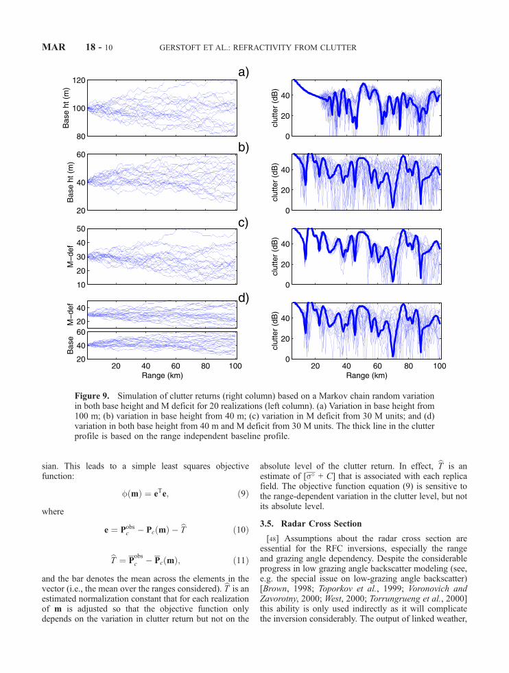
Figure 9. Simulation of clutter returns (right column) based on a Markov chain random variationin both base height and M deficit for 20 realizations (left column). (a) Variation in base height from100 m; (b) variation in base height from 40 m; (c) variation in M deficit from 30 M units; and (d)variation in both base height from 40 m and M deficit from 30 M units. The thick line in the clutterprofile is based on the range independent baseline profile.


wave, clutter and propagation models may eventually bebrought into the refractivity inversion algorithms. How-ever, assessing the goodness of the linked models shouldprecede that step and such investigations are only begin-ning [see Wagner et al., 2001].3.5.1. Range Dependence[49] Equation (7) shows that RFC is sensitive to s�(r).

If too much freedom is allowed for s�(r) then this willhamper our ability to estimate the refractivity profile.Because of nonlinearities it is possible to invert for somevariations in s�(r). We are at present neglecting all rangevariations in s�(r).[50] For the SPANDAR data the scale of variability of

the sea clutter radar cross section, over the ranges of 10to 60 km are on the order of several dB (section 5.4). Butthe propagation loss contour diagrams shows the 2-waypropagation loss over ranges as small as 10 km being onthe order of 30 dB or more (sections 5.1–5.3). Thus forthe cases considered here, the first-order problem is

developing a modeling of the refractive environmentthat can match the observed clutter intensifications.The horizontal variations in the sea-clutter radar crosssection are a second-order problem.[51] The relative contribution of sea clutter RCS vis a

vis that of the propagation is problem dependent. Exer-cising a sea clutter RCS model such as GIT will yieldthat the sensitivity of the sea clutter RCS to the windspeed is greater at low wind speeds (0–3 m/s) than at thewind speeds associated with the cases considered here(4–7 m/s). Thus in an environment such as the PersianGulf where surface based ducts are common but the windspeeds are typically lower, the horizontal variability ofthe sea clutter RCS may become more important.3.5.2. Grazing Angle[52] For vertical polarization there is still some ques-

tion as to whether the grazing angle dependence is y0, y4

or some value in between [see Barrick, 1998; Tatarskiand Charnotskii, 1998]. For inferring evaporation duct

Figure 10. Clutter returns as a function of range for different angles (top) and times (bottom). Theshaded area is the envelope of 13 returns in a 5� interval (i.e., 0.4� increment), and the dark line isthe median. In the top figure, the 5� angle intervals are for azimuths centered at 125�–160� at time13:00 EST. In the bottom figure, the time interval is 11:10–12:20 EST.


heights from radar sea echo, Rogers et al. [2000] foundthat while their data did not provide a definitive answerto the grazing angle dependency, the use of s / y0 in theduct height estimation algorithm generated better results.This model is chosen here.3.5.3. Radar Cross-Section Statistics[53] If the refractivity profiles measured via the heli-

copter are assumed accurate representations of the trueenvironment, it is possible to assess how well theinversion algorithm is estimating [s�(r) + C] withouthaving measured those quantities directly. We canmanipulate equations (7), (8), and (11) to obtain,

s� rð ÞþC½ � � T ¼ pobs rð Þ � 10 log rð Þ � bT þ 2L r;Mtrueð Þ:ð12Þ

T is the true value of the bias. Furthermore, by equation(11), the term p(r, Mtrue) � p(r, bM) drops out when weaverage over the ranges used in the computation of T togive:

s� þ C½ � � T ¼ 2 L r;Mtrueð Þ � 2 L�r; bM

ffi 2 L r;Mhelo�

� 2 L�r; bM

: ð13Þ

Themean and standard deviation of the right-hand sides ofequations (12)and(13) represent thebiasandstandarderrorof T in estimating [s�(r) + C] and [s� + C], respectively.

3.6. Optimization

[54] The Simulated Annealing/Genetic Algorithm code[Gerstoft, 1997; Gerstoft et al., 2000] is used to optimize

Figure 11. Inversion based on the clutter return shown in Figure 2 along azimuth 150�. (a) Theclutter return (dB) as observed by the radar data (black), the modeled return using the invertedprofile (red), and modeled return from the observed profile (blue); (b) observed profiles measuredfrom helicopter (blue and color-contour) and inverted profiles (red); (c) coverage diagram (dB)corresponding the inverted profiles; (d) coverage diagram (dB) based on helicopter profiles. (e)difference (dB) between coverage diagrams Figures 11c and 11d.


equation (9). The GA-search parameters were: parameterquantization 128 values; population size 64; reproduc-tion size 0.5; cross-over probability 0.05; number ofiterations for each population 2000; and number ofpopulations 10. Thus 20000 forward modeling runs wereperformed for each inversion. For further informationabout the use of GA for parameter estimation, seeGerstoft [1994].

4. Sensitivity

4.1. Sensitivity to Range-Independent Parameters

[55] Figure 8 shows the modeled clutter returns, equa-tion (7), as a function of range (x-axis) and variation ofindividual parameters ( y-axis). Clearly, changes in theinversion base height zb, thickness Dz, and mixed layerslope dM/dz, shift the location of intensifications. Addi-tionally, the size of the horizontal shift in the location ofan intensification increases nearly linearly as a functionof the intensification’s original range. One mighthypothesize that in performing the inversions, one reallyis inverting a super-parameter that is a linear combina-tion of zb, Dz, and dM/dz. As long as a surface duct iscreated, the M deficit (DM) is not an important param-eter. In the present simulation, this happens for a DM

value of about 20–30 M units. With a negative slope inthe mixed layer, a surface channel will always be createdcausing high clutter return. But for positive slopes, thecreation of surface duct depends on the zb, Dz, and DM.

4.2. Sensitivity to Range Dependency

[56] From the modified refractivity profiles in Figure 3,it is clear that these show a range (and temporal) depend-ence. This effect is simulated by modeling variations inrange as a Markov process as shown in Figure 9. Foreach kilometer, the profile was updated using a Gaussiandistribution with a standard deviation of 1 (m or Munits).[57] In the top pair of plots in Figure 9, the random

variations in zb about the starting value of 100 m providesome corruption to the major intensification between 45and 60 km, but the intensification is still recognizable.On the other hand, in the second pair of plots where thevariations is starting from zb = 40 m, features occurringbeyond about 30 km are difficult to associate withfeatures in the horizontally homogeneous case. Thisillustrates the state dependence of the response to param-eter variations. Clearly, the random variations in DM donot introduce as much variability as those in the baseheight. The lowest plots correspond to joint, independent

Figure 12. The clutter returns as observed by the radar data (black), the modeled returns using theinverted profile (red), and the modeled clutter returns for the helicopter profiles (blue, offset 20 dB)are shown for clutter maps 7–18 (corresponding to 10-min time intervals from 12:10–13:50 EST).The curves are normalized so that they have the same mean. The average absolute error inpredicting the clutter is 4.7 dB for the inversions and 8.9 dB for the helicopter profiles.


variations in the DM and base height. The variability isdominated by that induced from the base height.

4.3. Observed Azimuthal and Temporal Variabilityof Clutter Returns

[58] The envelopes and median values of Clutter-returndata from the SPANDAR are plotted in Figure 10. TheSPANDAR radar has an azimuthal resolution of 0.4�. Byanalyzing the returns over larger azimuthal resolution,5�, corresponding to 13 returns, an understanding of thevariation in clutter is obtained. The upper series of plotscorresponds to envelopes over different 5� sectors fromthe same clutter map. Plots in the lower series correspondto envelopes over a single 5� sector that were obtained at10-minute intervals. The broadening of the envelopeswith respect to range is possibly explained either byvariations in the mean value (with respect to range) ofthe parameters (Figure 8 illustrates a case), or by varia-tions in range as illustrated in Figure 9.

5. Inversion of SPANDAR Data

[59] The SPANDAR data, section 2, is used to dem-onstrate the feasibility of estimating the range-dependentrefractive structure. In section 5.1, a single clutter map isinverted, and in section 5.2, a sequence of 12 frames is

analyzed. This leads to a constraint on the M profile asdescribed in section 5.3.[60] The observed clutter data Pc

obs is taken from the150� radial and 10–60 km range using clutter mapssimilar to Figure 2. Twelve maps (clutter maps 7–18) at10-min intervals from 12:10–13:50 EST were used.

5.1. Analysis of a Single Frame

[61] Figure 11 summarizes the inversion and assess-ment of the inversion results for a single frame. First, theclutter Pc

obs along azimuth 150� and 10–60 km in rangeis extracted from the clutter map (Figure 2) and shown asa solid line in Figure 11a. Clutter-return intensificationsare seen at around 25, 35, and 45 km. Optimizing the fitbetween the replica Pc(m) and the observed data withrespect to the environmental parameters in Table 2 wascarried out. The best matching replica is shown as red,and for reference, the modeled clutter returns from thehelicopter profiles are shown in blue. The objectivefunction, equation (9), is only concerned with minimiz-ing the error and only indirectly is there optimization forthe location and number of peaks. The inversion canvisually be judged by examining how the peaks in thereplica are matched. Based on the location of maximaand minima in Figure 11a, the inversion only matcheswell at longer ranges.

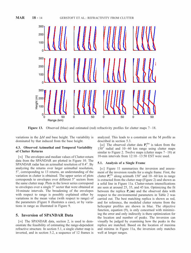
Figure 13. Observed (blue) and estimated (red) refractivity profiles for clutter maps 7–18.


[62] The second plot (Figure 11b) shows the estimatedrefractivity profiles (red) along with the helicopterrefractivity profiles (blue, color-contour). Because thisis an under determined problem, the best fit might notcorrespond to the true profile. An equivalent profile thatgives the best match to the clutter return is obtained.The next two plots show the modeled propagation lossfor the optimal environment and the helicopter profiles,respectively. The difference of these two (bottom plot)gives an indication of how well the inverted profile isable to predict the propagation loss. This plot has beenmedium filtered based on a 10 m 6 m box in rangeand height. Comparing this plot with the variationshown in Figure 5 indicates that the inversion is ofreasonable quality.

5.2. Inversion Without Constraints

[63] The clutter returns extracted from the clutter mapsare shown in Figure 12 (black). Notice that the clutterreturns vary significantly over a 10-min interval. Forreference, the clutter returns (blue) also are calculatedfrom the helicopter profiles closest in time. Four profilesof Figure 3 were used: helicopter profile 5 for cluttermaps 7–11, helicopter profile 6 for clutter-maps 12–13,

helicopter-profile 7 for clutter maps 14–17, and helicop-ter-profile 8 for clutter-map 18. It is clear that the clutterreturn modeled from the measured refractivity profilesdo not show a perfect match, but the main features arecaptured. It is expected that the nulls mainly are due todestructive interference in the wave propagation. Not allenvironmental information relevant for the propagationis captured in the helicopter-profiles, so these should notbe treated as ‘‘ground truth.’’[64] Based on the inversions, the range-dependent

profiles in Figure 13 were obtained. It can be seen thatthe estimated profiles (red) have a tendency to over-estimate the M excess, defined as M(0)–M(ztop), whereztop is the top of the trapping layer. This is because once awave is trapped in the duct, the value of the M excess isnot important, as illustrated in Figures 8b and 8d.[65] To assess the quality of the inversions, the corre-

sponding clutter returns (red lines in Figure 12) andcoverage diagrams (Figure 14) were generated.[66] The ratio between the fields based on the clutter

inversions (Figure 14) and the fields from the helicopterruns (frames 5–7 of Figure 4) is shown in Figure 15.While the difference in the first 50-m in height is quitesmall, the difference for the propagation above the duct

Figure 14. The coverage diagram (dB) based on the inverted profiles for clutter maps 7–18.


Figure 15. The difference (dB) between the fields from the inversion (Figure 14) and thehelicopter-based field (Figure 4).

Figure 16. Ambiguity surface (dB) of thickness versus M deficit based on data from clutter map18. The baseline environment is the solution of the unconstrained optimization. (a) With noconstraint; (b) with constraint (equation (6)). The dark blue area in Figure 16b indicates invalidsolutions. Red indicates a better fit.


is large. This is because the value of the M excess isimportant for how much energy radiates out of the ductbut is not well-determined by the inversion.

5.3. Inversion With Constraints

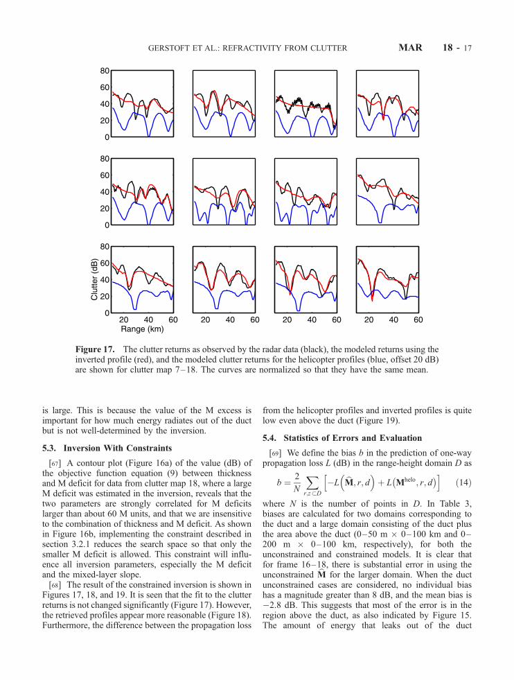
[67] A contour plot (Figure 16a) of the value (dB) ofthe objective function equation (9) between thicknessand M deficit for data from clutter map 18, where a largeM deficit was estimated in the inversion, reveals that thetwo parameters are strongly correlated for M deficitslarger than about 60 M units, and that we are insensitiveto the combination of thickness and M deficit. As shownin Figure 16b, implementing the constraint described insection 3.2.1 reduces the search space so that only thesmaller M deficit is allowed. This constraint will influ-ence all inversion parameters, especially the M deficitand the mixed-layer slope.[68] The result of the constrained inversion is shown in

Figures 17, 18, and 19. It is seen that the fit to the clutterreturns is not changed significantly (Figure 17). However,the retrieved profiles appear more reasonable (Figure 18).Furthermore, the difference between the propagation loss

from the helicopter profiles and inverted profiles is quitelow even above the duct (Figure 19).

5.4. Statistics of Errors and Evaluation

[69] We define the bias b in the prediction of one-waypropagation loss L (dB) in the range-height domain D as

b ¼ 2

N

Xr;z�D

�L bM; r; d �

þ L Mhelo; r; d� h i

ð14Þ

where N is the number of points in D. In Table 3,biases are calculated for two domains corresponding tothe duct and a large domain consisting of the duct plusthe area above the duct (0–50 m 0–100 km and 0–200 m 0–100 km, respectively), for both theunconstrained and constrained models. It is clear thatfor frame 16–18, there is substantial error in using theunconstrained bM for the larger domain. When the ductunconstrained cases are considered, no individual biashas a magnitude greater than 8 dB, and the mean bias is�2.8 dB. This suggests that most of the error is in theregion above the duct, as also indicated by Figure 15.The amount of energy that leaks out of the duct

Figure 17. The clutter returns as observed by the radar data (black), the modeled returns using theinverted profile (red), and the modeled clutter returns for the helicopter profiles (blue, offset 20 dB)are shown for clutter map 7–18. The curves are normalized so that they have the same mean.


depends on the value of the M deficit, but the totalenergy in the duct is nearly constant as long as the Mdeficit is so large that the energy is trapped. When theconstrained model is used, the mean and standarddeviation of the biases across the data are small (bothless than 4 dB).[70] The helicopter profiles are not easy to obtain in

practice. In fact, having a single Radiosonde or rock-etsonde at the midpoint of the transmission path ofinterest might be considered a best case scenario. Asingle sounding is simulated by assuming the verticalrefractivity profile at all ranges equal to the midrangehelicopter refractivity profile. Our benchmark is theaccuracy of these ‘‘range-independent’’ environmentsin estimating the propagation loss that is predicted usingthe range-dependent soundings. The benchmark was notvery sensitive to which profile was used for the range-independent environment.[71] Error statistics for 2-way propagation loss (dB)

for the RFC algorithm and the benchmark, consideringthe duct domains (0–50 m 0–100 km) and a largedomain (0–200 m 0–100 km), are given in Table 4.The time delay is obtained by using an older Radio-sonde. It is seen that the errors increase with time

delay; the constrained and unconstrained gives aboutthe same error; and the larger domain gives a slightlylarger error. For the cases considered, Propagation-lossvalues based on radar-inferred refractivity structuresapproach what might be obtained using a single repre-sentative sounding.[72] We now consider how good the a priori knowl-

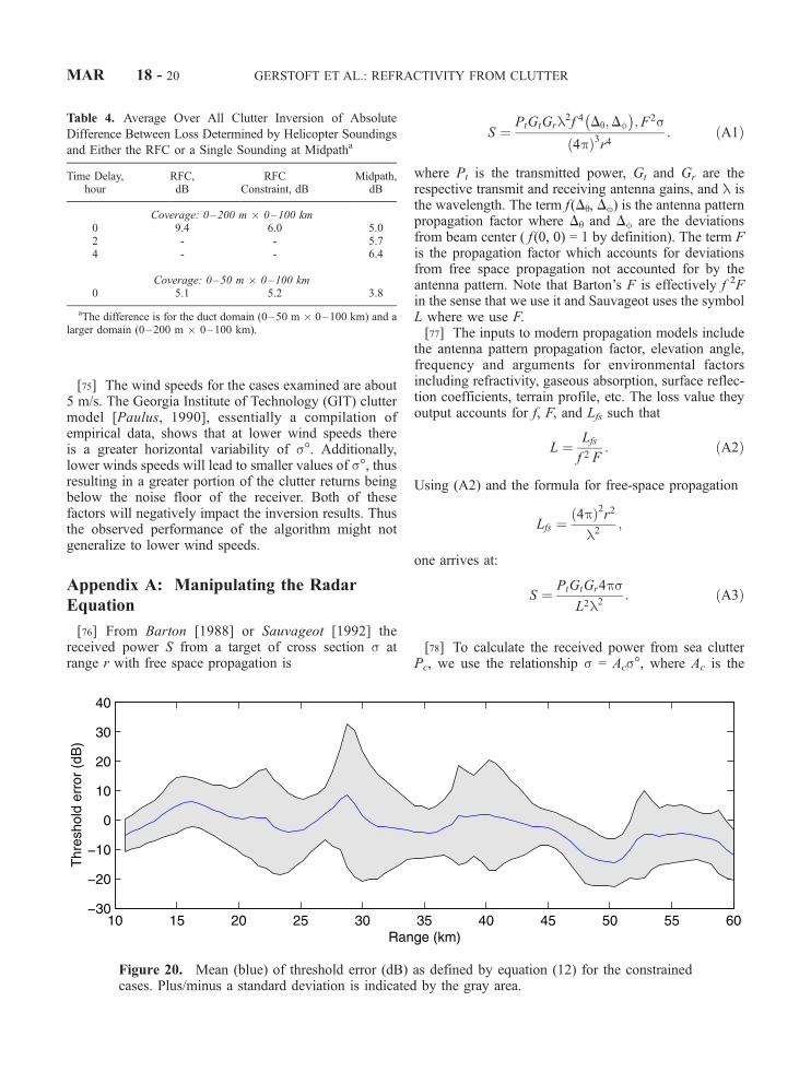
edge of s� would have to be in order to be an aid forthe inversion. Figure 20 is a plot of the mean andenvelope defined by the standard deviation of equation(12) over the constrained cases. The trend that thestandard deviation decreases with range is realistic; itimplies that s� may be decreasing about 5 dB over the50-km range. The range-averaged value of the mean(corresponding to equation (13)) is �2.8 dB, represent-ing the amount bT is underestimating [s� + C]. This isconsistent with over estimating duct strength. The valueof T depends on parameter vector m, equation (11), andvaries over several decades (dB). Clearly, the bT (bm) aretightly distributed about the true values of [s� + C].Given the small uncertainty in [s� + C], it might bedifficult to use a priori estimates of [s� + C] (theformer term presumably calculated from wind fieldsgenerated by a numerical weather prediction model)

Figure 18. Observed (blue) and estimated (red) refractivity profiles for clutter map 7–18.


with sufficient accuracy to improve the inversionresults.

6. Summary

[73] An implementation for the inference of refractivityparameters from radar clutter has been described. Amulti-parameter range-dependent parameterization wasintroduced and the use of a genetic algorithm via theSAGA inversion code was employed to handle the largesearch space. We find that within the duct itself, theaccuracy of the radar-inferred propagation-loss valuesapproaches that of loss values calculated using a midpathsounding. This finding is based on an analysis that wouldtend to favor the midpath sounding. But, the ability ofthe radar-inferred loss values to estimate the loss valuesin the shadow zone above the duct is more limited. It isdemonstrated that inclusion of prior information allevi-ates this problem to a large degree.[74] The parameterization and search bounds that were

used could easily accommodate refractivity profilesfound in other regions of the world. Furthermore, asthe sensitivity examination in section 4 showed, therelatively low ducts in these data tend to stress theinversion algorithm more than the alternative of higher

ducts. Thus we have no reason to suspect that theperformance of the algorithm will degrade when imple-mented using data where the typical refractivity struc-tures differ from the cases examined here.

Figure 19. The difference (dB) between the fields from the inversion and the helicopter-basedfields (Figure 4).

Table 3. Two-Way Propagation Loss Biasa

Clutter Map 0–200 m, U 0–200 m, C 0–50 m, U 0–50 m, C

7 1.2 �2.6 �2.3 �0.88 �0.6 �1.4 �0.7 �0.99 �3.2 �3.3 �0.9 5.010 5.0 3.8 �3.3 �3.011 1.8 2.6 �2.8 �3.112 6.0 4.2 �7.7 �8.113 6.8 1.9 �7.8 �6.714 4.0 1.0 2.7 3.315 �0.0 1.6 �1.0 �0.216 17.3 2.6 �1.9 1.117 25.5 0.6 �1.6 1.818 29.2 �1.0 �5.8 0.1m 7.7 0.8 �2.8 �1.0s 10.5 2.4 3.0 3.8

aAveraged difference in 2-way propagation loss calculations based onradar-inferred refractivity and calculated from the helicopter soundings.The duct domain (0–50 m 0–100 km) and a larger domain (0–200m 0–100 km) are considered as unconstrained (U) and constrained(C) solutions.


[75] The wind speeds for the cases examined are about5 m/s. The Georgia Institute of Technology (GIT) cluttermodel [Paulus, 1990], essentially a compilation ofempirical data, shows that at lower wind speeds thereis a greater horizontal variability of s�. Additionally,lower winds speeds will lead to smaller values of s�, thusresulting in a greater portion of the clutter returns beingbelow the noise floor of the receiver. Both of thesefactors will negatively impact the inversion results. Thusthe observed performance of the algorithm might notgeneralize to lower wind speeds.

Appendix A: Manipulating the Radar

Equation

[76] From Barton [1988] or Sauvageot [1992] thereceived power S from a target of cross section s atrange r with free space propagation is

S ¼PtGtGrl2f 4 Dq;Df

� ;F2s

4pð Þ3r4: ðA1Þ

where Pt is the transmitted power, Gt and Gr are therespective transmit and receiving antenna gains, and l isthe wavelength. The term f (Dq, Df) is the antenna patternpropagation factor where Dq and Df are the deviationsfrom beam center ( f (0, 0) = 1 by definition). The term Fis the propagation factor which accounts for deviationsfrom free space propagation not accounted for by theantenna pattern. Note that Barton’s F is effectively f 2Fin the sense that we use it and Sauvageot uses the symbolL where we use F.[77] The inputs to modern propagation models include

the antenna pattern propagation factor, elevation angle,frequency and arguments for environmental factorsincluding refractivity, gaseous absorption, surface reflec-tion coefficients, terrain profile, etc. The loss value theyoutput accounts for f, F, and Lfs such that

L ¼ Lfs

f 2 F: ðA2Þ

Using (A2) and the formula for free-space propagation

Lfs ¼4pð Þ2r2

l2;

one arrives at:

S ¼ PtGtGr4psL2l2

: ðA3Þ

[78] To calculate the received power from sea clutterPc, we use the relationship s = Acs�, where Ac is the

Figure 20. Mean (blue) of threshold error (dB) as defined by equation (12) for the constrainedcases. Plus/minus a standard deviation is indicated by the gray area.

Table 4. Average Over All Clutter Inversion of Absolute

Difference Between Loss Determined by Helicopter Soundings

and Either the RFC or a Single Sounding at Midpatha

Time Delay,hour

RFC,dB

RFCConstraint, dB

Midpath,dB

Coverage: 0–200 m 0–100 km0 9.4 6.0 5.02 - - 5.74 - - 6.4

Coverage: 0–50 m 0–100 km0 5.1 5.2 3.8

aThe difference is for the duct domain (0–50 m 0–100 km) and alarger domain (0–200 m 0–100 km).


illuminated area and s� is the sea clutter’s normalizedradar cross section, to rewrite equation (A3) as

Pc ¼PtGtGr4pAcs�

L2l2: ðA4Þ

At low grazing angles, Ac is a linear function of r, thuswe can rewrite equation (A4) in the form

Pc ¼Cs�rL2

: ðA5Þ

where C accounts for all of the constant terms in (A4).Letting the symbols Pc, C, s�, and L represent theassociated values in dB as opposed to real numbers, wecan rewrite equation (A5) as

Pc ¼ �2Lþ s� þ 10log10 rð Þ þ C: ðA6Þ

[79] Acknowledgments. This research was supported bythe Office of Naval Research, Codes 321 and 322.

References

Anderson, R., S. Vasudevan, J. Krolik, and L. T. Rogers, Max-

imum a posteriori refractivity estimation from radar clutter

using a Markov model for microwave propagation, paper

presented at the International Geoscience and Remote Sen-

sing Symposium, Sydney, Australia, Int. of Electr. and Elec-

tron. Eng., New York, July 2001.

Barrick, D. E., Grazing angle behavior of scatter and propaga-

tion above any rough surface, IEEE Antennas Propag.,

46(1), 73–83, 1998.

Barrios, A. E., A terrain parabolic equation model for propaga-

tion in the troposphere, IEEE Trans. Antennas Propag., 42,

90–98, 1994.

Barton, D. K., Modern Radar System Analysis, Artech House,

Norwood, Mass., 1988.

Brown, G. S., Special issue on low-grazing-angle backscatter

from rough surfaces, IEEE Trans. Antennas Propag., 46(1),

1–2, 1998.

Dockery, G. D., Development and use of electromagnetic para-

bolic equation propagation models for US Navy applica-

tions, Johns Hopkins APL Tech. Dig., 19, 283–292, 1998.

Gerstoft, P., Inversion of seismoacoustic data using genetic

algorithms and a posteriori probability distributions,

J. Acoust. Soc. Am., 95, 770–782, 1994.

Gerstoft, P., SAGA Users Guide 2.0: An Inversion Software

Package, SM-333, SACLANT Undersea Res. Cent., La

Spezia, Italy, 1997. (Available at http://www-mpl.ucsd.edu/

people/gerstoft/saga/saga.html.)

Gerstoft, P., and C. F. Mecklenbrauker, Ocean acoustic inver-

sion with estimation of a posteriori probability distributions,

J. Acoust. Soc. Am., 104, 808–819, 1998.

Gerstoft, P., D. F. Gingras, L. T. Rogers, and W. S. Hodgkiss,

Estimation or radio refractivity structure using matched field

array processing, IEEE Trans. Antennas Propag., 48, 345–

356, 2000.

Goldhirsh, J., and D. Dockery, Propagation factor errors due to

the assumption of lateral homogeneity, Radio Sci., 33(2),

239–249, 1998.

Gossard, E. E., and R. G. Strauch, Radar Observations of Clear

Air and Clouds, Elsevier Sci., New York, 1983.

Haack, T., and S. D. Burk, Summertime marine refractivity

conditions along coastal California, J. Appl. Meteorol., 40,

673–687, 2001.

Krolik, J. L., and J. Tabrikian, Tropospheric refractivity estima-

tion using radar clutter from the sea surface, in Proceedings of

the 1997 Battlespace Atmospherics Conference, SPAWAR Sys.

Command Tech. Rep. 2989, 635–642, Space and Nav. War-

fare Sys. Command Cent., San Diego, Calif., March 1998.

Levy, M. F., Parabolic Equation Methods for Electromagnetic

Wave Propagation, Inst. of Electr. Eng., London, 2000.

Patterson, W., Ducting Climatology Summary, SPAWAR Sys.

Cent., San Diego, Calif., 1992.

Paulus, R. A., Evaporation duct effects on sea clutter, Radio

Sci., 38(11), 1765–1771, 1990.

Richter, J. H., Structure, variability, and sensing of the coastal

environment, in Proceedings of the AGARD SPP Sympo-

sium on Propagation Assessments in Coastal Environments,

Bremerhaven, Germany, pp. 1.1–7.14, NATO AGARD,

Neuilly-sur-Seine, France, Feb. 1995.

Rogers, L. T., Likelihood estimation of tropospheric duct para-

meters from horizontal propagation measurements, Radio

Sci., 32, 79–92, 1997.

Rogers, L. T., C. P. Hattan, and J. K. Stapleton, Estimating

evaporation duct heights from radar sea clutter, Radio Sci.,

35(4), 955–966, 2000.

Rowland, J. R., G. C. Konstanzer, M. R. Neves, R. E. Miller,

J. H. Meyer, and J. R. Rottier, SEAWASP: Refractivity char-

acterization using shipboard sensors, in Proceedings of the

Battlespace Atmospherics Conference, Tech. Doc. 2938, pp.

155–164, RDT&E Div., Nav. Command Control and Ocean

Surv. Cent., San Diego, Calif., Dec. 1996.

Sauvageot, H., Radar Meteorology, Artech House, Norwell,

Mass., 1992.

Stahl, R. W., and D. A. Crippen, An Experimenters Guide to the

NASA Atmospheric Sciences Research Facility, Goddard

Space Flight Cent., Wallops Flight Facil., Wallops Is., Va.,

March 1994.

Stull, R. B., An Introduction to Boundary Layer Meteorology,

Kluwer Acad., New York, 1998.

Tatarski, V. I., and M. Charnotskii, On the behavior of scatter-

ing from a rough surface for small grazing angles, IEEE

Antennas Propag., 46(1), 67–72, 1998.

Tarantola, A., Inverse Problem Theory: Methods for Data Fit-

ting and Model Parameter Estimation, Elsevier Sci., New

York, 1987.

Toporkov, J. V., R. S. Awadallah, and G. S. Brown, Issues related

to the use of a Gaussian-like incident field for low-grazing-

angle scattering, J. Opt. Soc. Am., 16, 176–187, 1999.


Torrungrueng, D., H.-T. Chou, and J. T. Johnson, A novel

acceleration algorithm for the computation of scattering

from two-dimensional large-scale perfectly conducting ran-

dom rough surfaces with the forward-backward method,

IEEE Trans. Geosci. Remote Sens., 38, 1656–1668, 2000.

Voronovich, A. G., and V. U. Zavorotny, The effect of steep

sea-waves on polarization ratio at low grazing angles, IEEE

Trans. Geosci. Remote Sens., 38, 366–373, 2000.

Wagner, L. J., L. T. Rogers, S. D. Burk, and T. Haack, Island

wake impact on evaporation duct height and sea clutter in

the lee of Kauai, paper presented at International Geoscience

and Remote Sensing Symposium, Sydney, Australia, Int. of

Electr. and Electron. Eng., New York, July 2001.

West, J. C., Integral equation formulation for iterative calcula-

tion of scattering from lossy rough surfaces, IEEE Trans.

Geosci. Remote Sens., 38, 1609–1615, 2000.

Wyngaard, J. C., N. L. Seaman, S. J. Kimmel, M. Otte, X. Di,

and K. E. Gilbert, Concepts, observations, and simulation of

refractive index turbulence in the lower atmosphere, Radio

Sci., 36(4), 643–670, 2001.

��P. Gerstoft and W. S. Hodgkiss, Marine Physical Laboratory,

University of California, San Diego, La Jolla, CA 92093-0238,

USA. ([email protected]; [email protected])

J. L. Krolik, Electrical and Computer Engineering, Duke

University, Durham, NC 27708, USA. ( [email protected])

L. T. Rogers, Atmospheric Propagation Branch, SPAWAR

Systems Center, San Diego, CA 92152, USA. (trogers@spawar.

navy.mil)


inversion for refractivity parameters from radar sea...

Documents