Inversion imaging of the Sun-Earth System

Damien Allain, Cathryn Mitchell, Dimitriy Pokhotelov, Manuchehr Soleimani, Paul Spencer, Jenna Tong, Ping Yin, Bettina Zapfe

Invert, Dept of E & E Engineering, University of Bath, UK

BICS, September 2007

Tomography and the ionosphere

• Outline the basic problem

GPS imaging of electron density

• large-scale slow moving (mid/low latitude)

• medium-scale fast moving (high latitude)

• high-resolution imaging

• small-scale structure

System applications

Next steps

Plan

The ionosphere

Tenuous atmosphere above 100 km – ionised by EUV

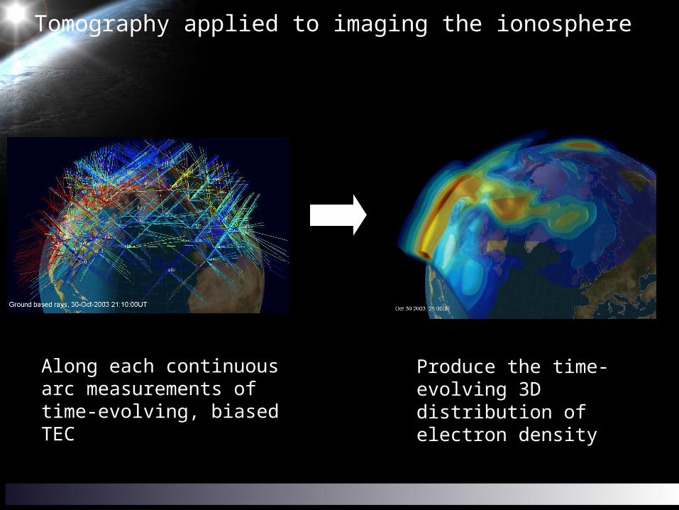
Along each continuous arc measurements of time-evolving, biased TEC

Produce the time-evolving 3D distribution of electron density

Tomography applied to imaging the ionosphere

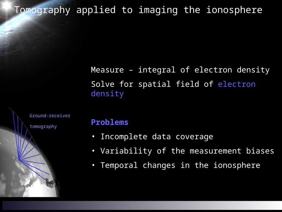
Ground-receiver

tomography

Measure – integral of electron density

Solve for spatial field of electron density

Problems

• Incomplete data coverage

• Variability of the measurement biases

• Temporal changes in the ionosphere

Tomography applied to imaging the ionosphere

?

?

?

?

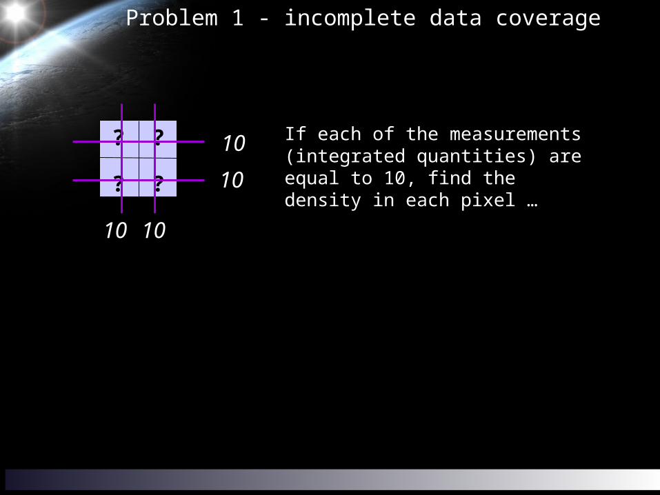
If each of the measurements (integrated quantities) are equal to 10, find the density in each pixel …

10

10

1010

Problem 1 - incomplete data coverage

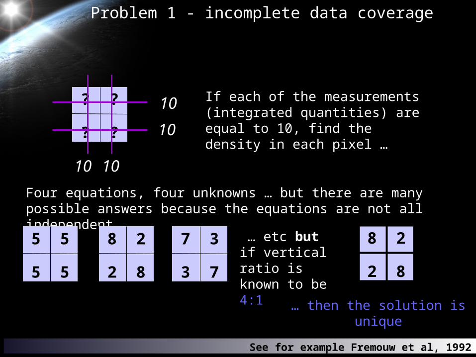
Four equations, four unknowns … but there are many possible answers because the equations are not all independent

?

?

?

?

5

5

5

5

8

8

2

2

7

7

3

3

… etc but if vertical ratio is known to be 4:1

Problem 1 - incomplete data coverage

10

10

1010

8

8

2

2

… then the solution is unique

If each of the measurements (integrated quantities) are equal to 10, find the density in each pixel …

See for example Fremouw et al, 1992

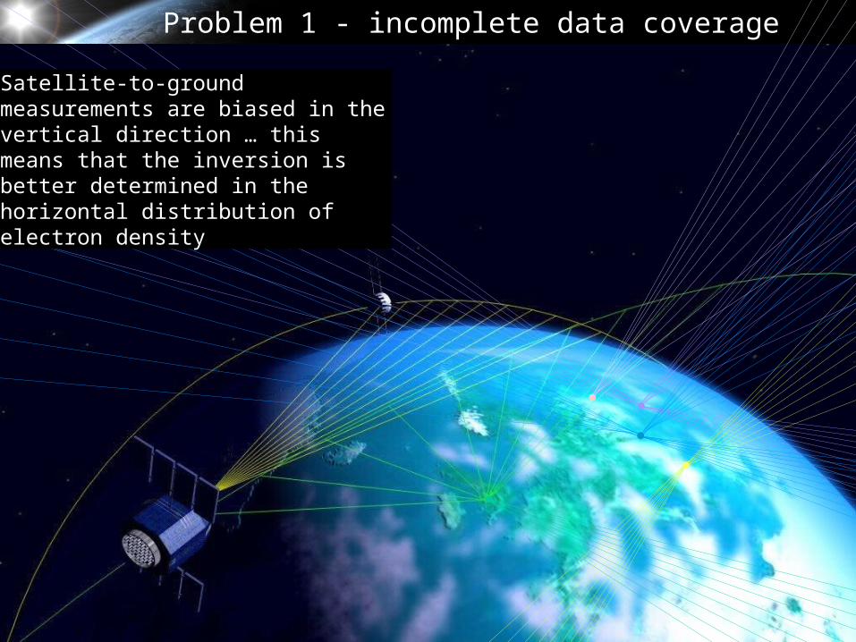
Satellite-to-ground measurements are biased in the vertical direction … this means that the inversion is better determined in the horizontal distribution of electron density

Problem 1 - incomplete data coverage

Low peak height small scale height High peak height large scale height

Example of basis set constraints of MIDAS

h

EOF1

EOF2

EOF3

Problem 1 - incomplete data coverage

?

?

?

?

Problem 2 – variable measurement biases

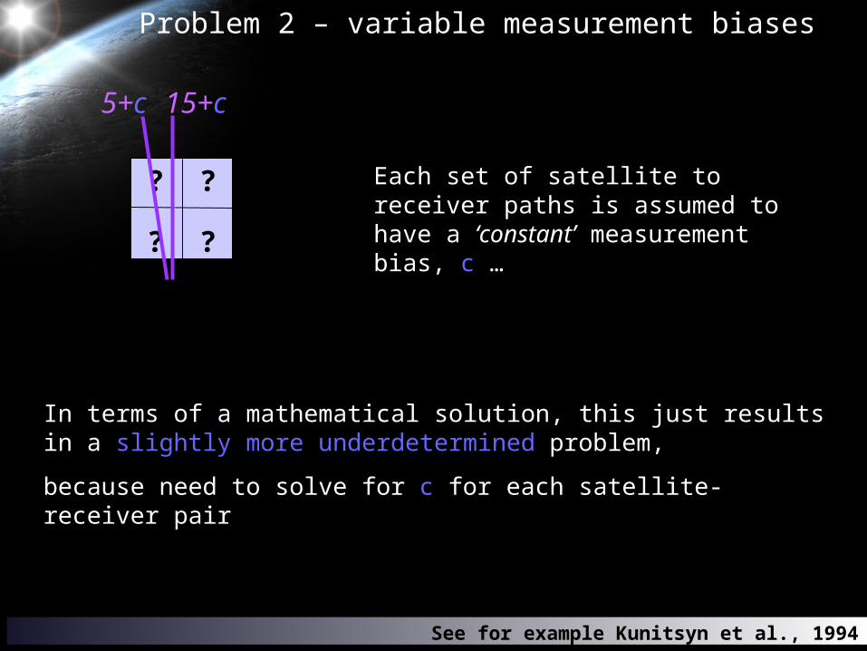
Each set of satellite to receiver paths is assumed to have a ‘constant’ measurement bias, c …

In terms of a mathematical solution, this just results in a slightly more underdetermined problem,

because need to solve for c for each satellite-receiver pair

5+c 15+c

See for example Kunitsyn et al., 1994

NmF2 from ground based data?

20 TECu

Hei

gh

t (k

m)

TECu

TECu

Large differences in the profile still result in small TEC changes …

… so we need to use the differential phase not the

calibrated code observations

Problem 2 – variable measurement biases

?

?

?

?

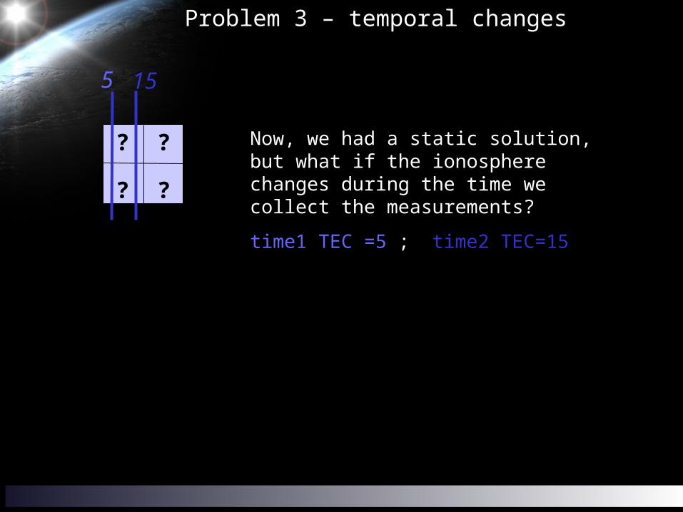
Problem 3 – temporal changes

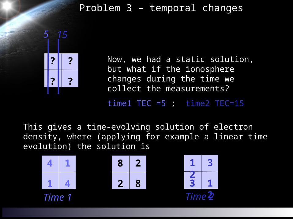
Now, we had a static solution, but what if the ionosphere changes during the time we collect the measurements?

time1 TEC =5 ; time2 TEC=15

5 15

?

?

?

?

4

4

1

1

Now, we had a static solution, but what if the ionosphere changes during the time we collect the measurements?

time1 TEC =5 ; time2 TEC=15

5 15

This gives a time-evolving solution of electron density, where (applying for example a linear time evolution) the solution is

8

8

2

2

12

12

3

3

Time 1 Time 2

Problem 3 – temporal changes

Problem 4 – uneven data coverage

Some form of regularisation e.g. spherical harmonics

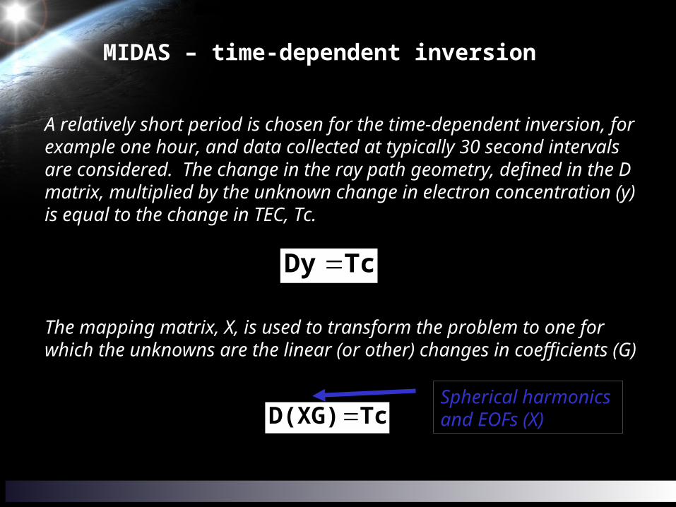
A relatively short period is chosen for the time-dependent inversion, for example one hour, and data collected at typically 30 second intervals are considered. The change in the ray path geometry, defined in the D matrix, multiplied by the unknown change in electron concentration (y) is equal to the change in TEC, Tc.

The mapping matrix, X, is used to transform the problem to one for which the unknowns are the linear (or other) changes in coefficients (G)

TcDy

TcD(XG)

MIDAS – time-dependent inversion

Spherical harmonics and EOFs (X)

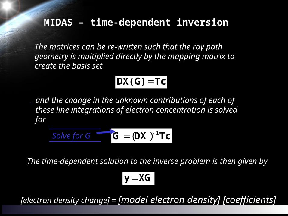
The time-dependent solution to the inverse problem is then given by

The matrices can be re-written such that the ray path geometry is multiplied directly by the mapping matrix to create the basis set

and the change in the unknown contributions of each of these line integrations of electron concentration is solved for

.

TcDX(G)

TcDXG 1)(

MIDAS – time-dependent inversion

XGy

[electron density change] = [model electron density] [coefficients]

Solve for G

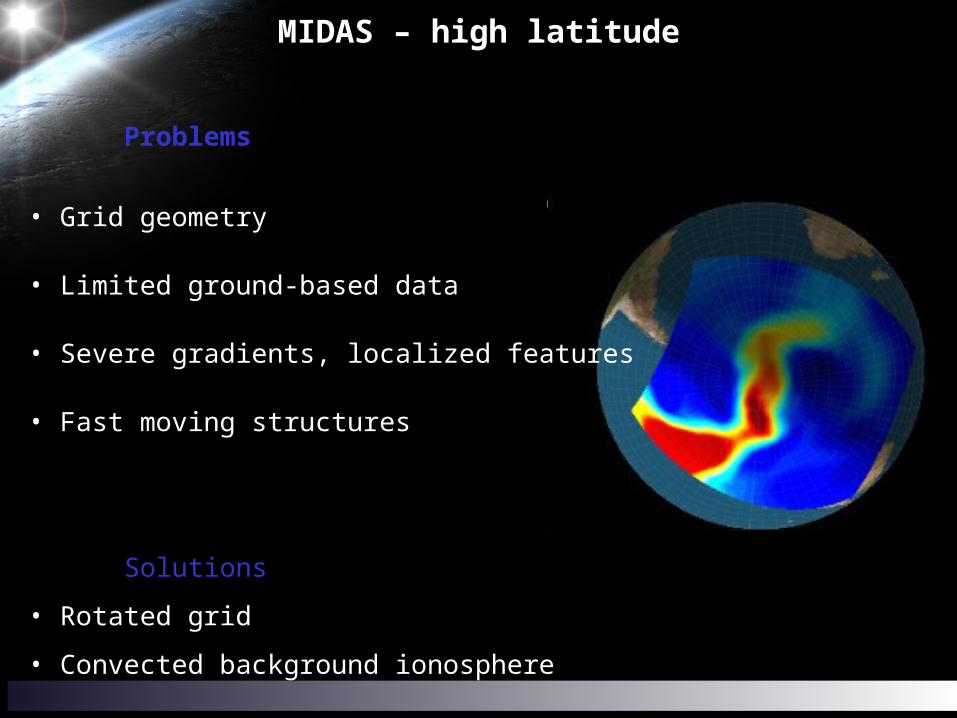
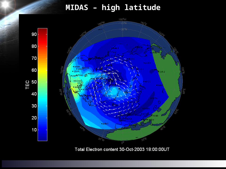
MIDAS – high latitude

Problems

• Grid geometry

• Limited ground-based data

• Severe gradients, localized features

• Fast moving structures

Solutions

• Rotated grid

• Convected background ionosphere

zHx r

1 tAxx

QAAPP T

t 1

1)( RHPHPHK TT

)( HxzKxx t

PKHIP )( t

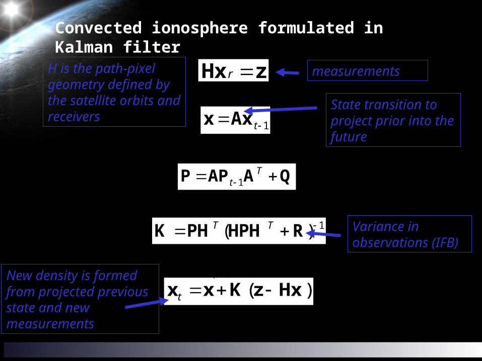
State transition to project prior into the future

Convected ionosphere formulated in Kalman filter

New density is formed from projected previous state and new measurements

H is the path-pixel geometry defined by the satellite orbits and receivers

measurements

Variance in observations (IFB)

MIDAS – high latitude

E-field from Weimer

MIDAS – high latitude

Magnetic field from IGRF

MIDAS – high latitude

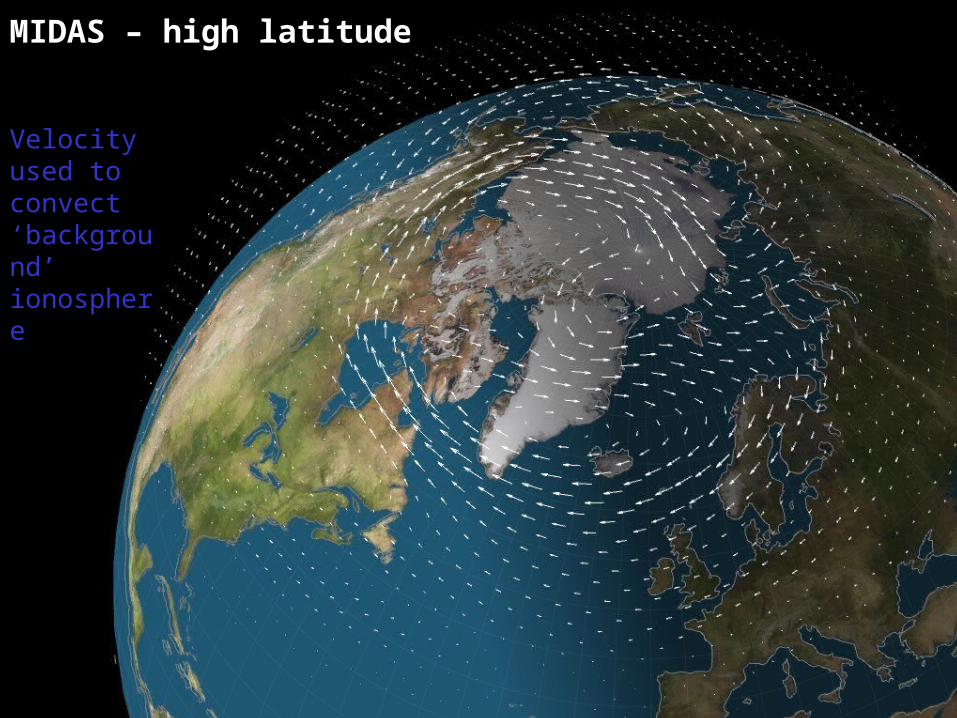
Velocity used to convect ‘background’ ionosphere

MIDAS – high latitude

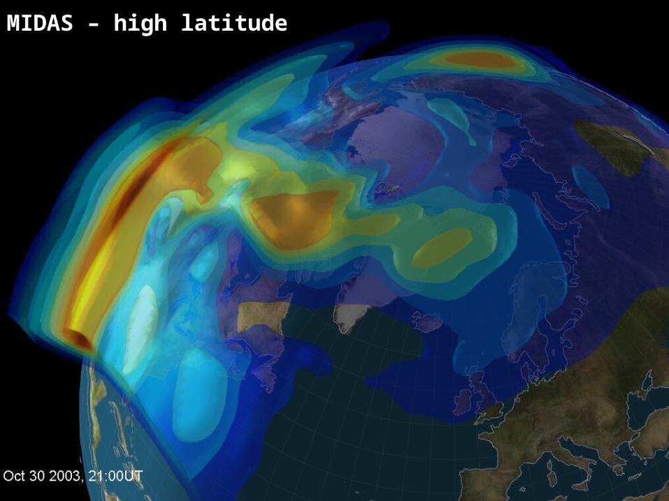
MIDAS – high latitude

MIDAS – high latitude

MIDAS – high latitude

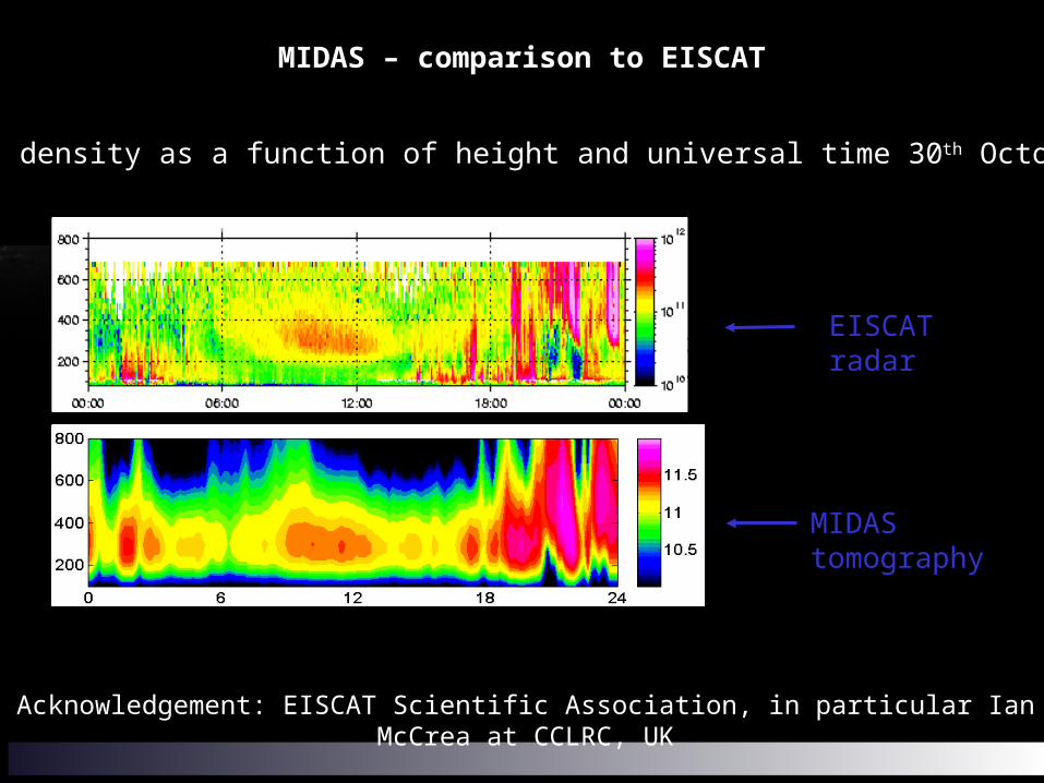
MIDAS – comparison to EISCAT

Acknowledgement: EISCAT Scientific Association, in particular Ian McCrea at CCLRC, UK

Electron density as a function of height and universal time 30th October 2003

EISCATradar

MIDAStomography

Conjugate plasma controlled by electric field

Arctic Antarctic

GPS data-sharing collaboration through International Polar Year 2007-2008

Extension of imaging to Antarctica

High-resolution imaging

In collaboration with J-P Luntama, FMI

In collaboration with J-P Luntama, FMI

High-resolution imaging

Equatorial imaging and GPS Scintillation – South America and Europe

In collaboration with Cornell University, USA

GPS

Ionosphere multi-scale problems – system effects

Credit: ESA

• Perturbs the signal propagation speed proportional to total electron content – tens of metres error at solar maximum

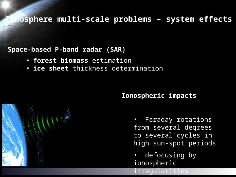
Space-based P-band radar (SAR)

• forest biomass estimation• ice sheet thickness determination

Ionosphere multi-scale problems – system effects

Ionospheric impacts

• Faraday rotations from several degrees to several cycles in high sun-spot periods

• defocusing by ionospheric irregularities

Tomography and the ionosphere

GPS imaging of electron density

System applications

Next steps …

Summary and Further Work

NASA movie - CME Sun-Earth connections

Goal – to nowcast and forecast the Sun-Earth System

Models –

• Do we know all of the physics of the Sun-Earth System?

• Can we simplify it into a useful Sun-Earth model?

• Computational – how can we minimise the computational costs?

Multi-scale data assimilation (temporal and spatial) will be essential

Next steps

Credit to ESA