Inverting In-Water Reflectance

Eric Rehm

Darling Marine Center, Maine

30 July 2004

Inverting In-Water Radiance

Estimation of the absorption and backscattering coefficients from in-water radiometric measurements

Stramska, Stramski, Mitchell, Mobley

Limnol. Oceanogr. 45(3), 2000, 629-641

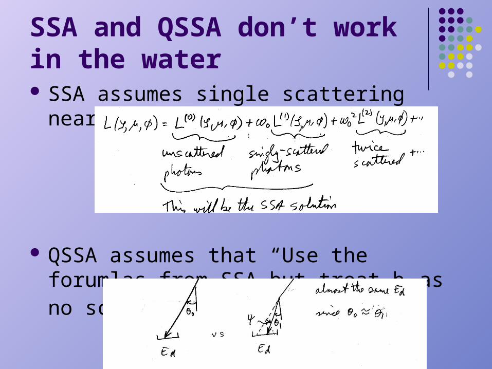
SSA and QSSA don’t work in the water SSA assumes single scattering near surface

QSSA assumes that “Use the forumlas from SSA but treat bf as no scattering at all.

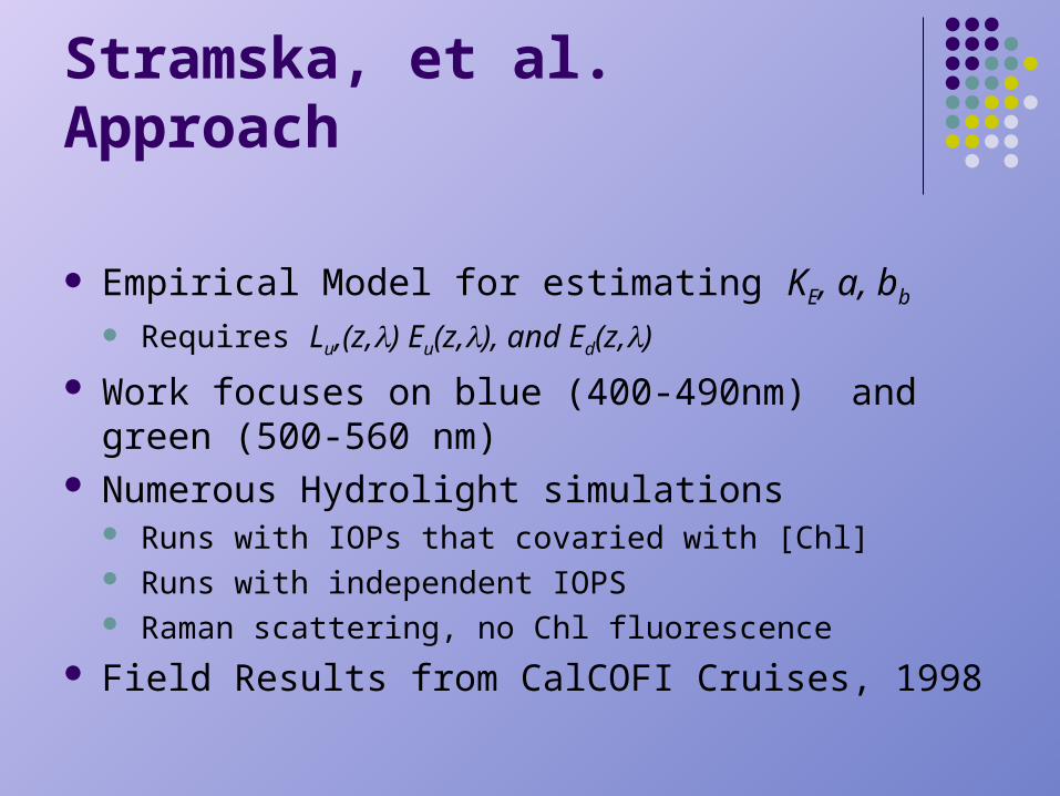
Stramska, et al. Approach

Empirical Model for estimating KE, a, bb Requires Lu,(z,) Eu(z,), and Ed(z,)

Work focuses on blue (400-490nm) and green (500-560 nm)

Numerous Hydrolight simulations Runs with IOPs that covaried with [Chl] Runs with independent IOPS Raman scattering, no Chl fluorescence

Field Results from CalCOFI Cruises, 1998

Conceptual Background

Irradiance Reflectance R = Eu/Ed Just beneath water: R(z=0-) = f *bb/a

f 1/0 where 0=cos()

Also (Timofeeva 1979)

Radiance Reflectance RL=Lu/Ed

Just beneath the water RL(z=0-) =(f/Q)(bb/a), where Q=(Eu/Lu

)

f and Q covary f/Q less sensitive to angular distribution of light

1R

Conceptual Background Assume

R(z) =Eu/Ed bb(z)/a(z)

RL(z) =Lu/Ed bb(z)/a(z), not sensitive to directional structure of light field

RL/R can be used to estimate Many Hydrolight runs to build in-water empirical model

KE can be computed from Ed, Eu Gershuns Law a=KE* Again, many Hydrolight runs to build in-water

empirical model of bb(z) ~ a(z)*RL(z)

1

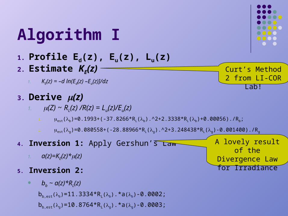
Algorithm I1. Profile Ed(z), Eu(z), Lu(z)2. Estimate KE(z)

1. KE(z) = –d ln(Ed(z) –Eu(z)]/dz

3. Derive (z)1. (Z) ~ RL(z) /R(z) = Lu(z)/Eu(z)

1. est(b)=0.1993+(-37.8266*RL(b).^2+2.3338*RL(b)+0.00056)./Rb;

2. est(g)=0.080558+(-28.88966*RL(g).^2+3.248438*RL(g)-0.001400)./Rg

4. Inversion 1: Apply Gershun’s Law

1. a(z)=KE(z)*(z)

5. Inversion 2:

bb ~ a(z)*RL(z)

bb,est(b)=11.3334*RL(b).*a(b)-0.0002;

bb,est(g)=10.8764*RL(g).*a(g)-0.0003;

Curt’s Method 2 from LI-COR Lab!

A lovely result of the Divergence Law for

Irradiance

Algorithm II Requires knowledge of attenuation coefficient c Regress simulated vs Lu/Eu for variety of

bb/b and 0 = b/c best=0.5*(b1+b2)

b1=c – aest (underestimate)

b2=bw + (bb,est-.5*bw)/0.01811 (overestimate)

Compute0 = best/c Retrieve based on bb/b:

2,est = mi(0)*(Lu/Eu) + bi (0)

As before Use 2,est to retrieve a Use RL and a to retrieve bb

Model Caveats

Assumes inelastic scattering and internal light sources negligible Expect errors in bb to increase with depth and

decreasing Chl. Limit model to top 15 m of water column

Blue (400-490 nm) & Green (500-560 nm) Used Petzold phase function for simulations

Acknowledge that further work was needed here

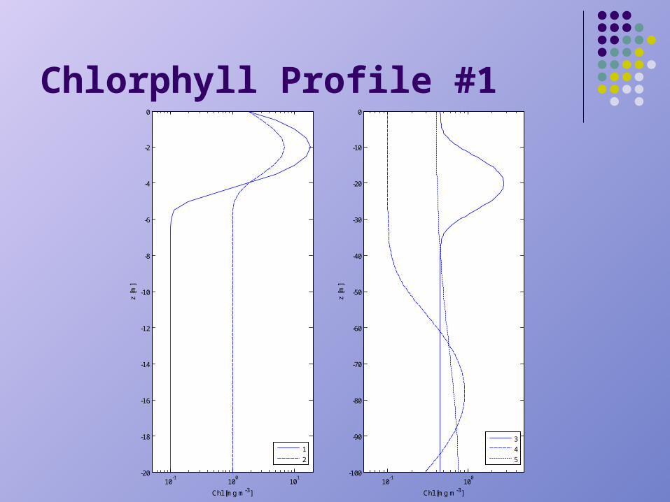
My Model #1

Hydrolight Case 1 Raman scattering only Chlorophyll profile with 20 mg/L max at 2 m Co-varying IOPs 30 degree sun, 5 m/s wind, bb/b=.01

10-1

100

101

-20

-18

-16

-14

-12

-10

-8

-6

-4

-2

0

Chl [mg m-3]

z [m

]

10-1

100

-100

-90

-80

-70

-60

-50

-40

-30

-20

-10

0

Chl [mg m-3]

z [m

]

3

4

5

1

2

Chlorphyll Profile #1

AOP/IOP Retrieval Results

0.6 0.65 0.7 0.75 0.8

0.6

0.65

0.7

0.75

0.8

est

0.1 0.2 0.3 0.4

0.05

0.1

0.15

0.2

0.25

0.3

0.35

0.4

0.45

a (m-1)

a est (

m-1

)

0.01 0.02 0.03 0.04 0.05

0.005

0.01

0.015

0.02

0.025

0.03

0.035

0.04

0.045

0.05

bb (m-1)

b b,es

t (m

-1)

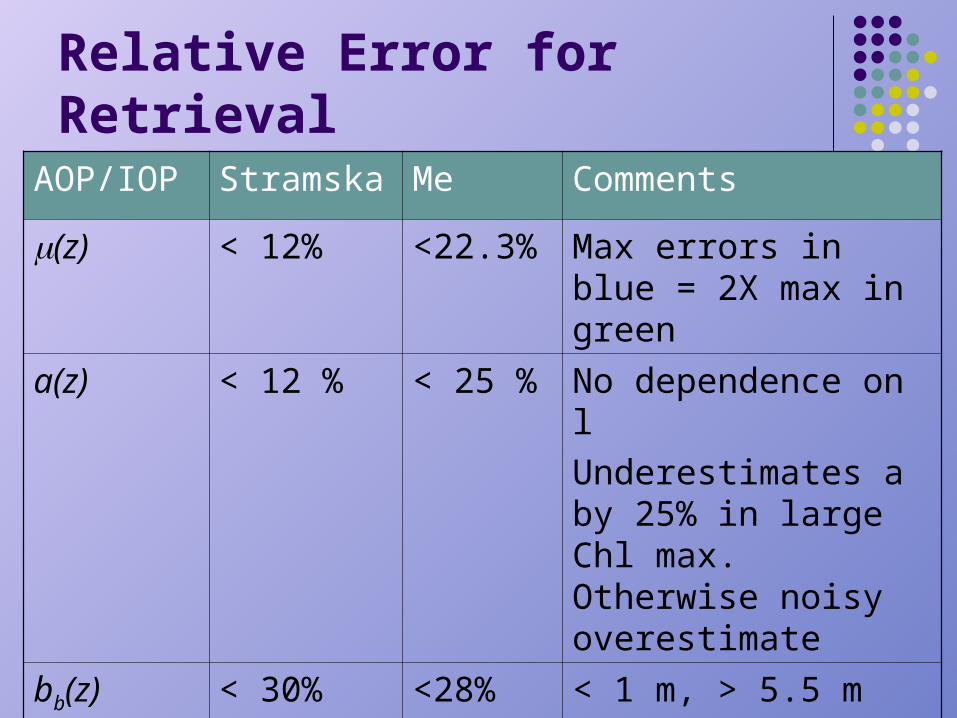
Relative Error for RetrievalAOP/IOP Stramska Me Comments

(z) < 12% <22.3% Max errors in blue = 2X max in green

a(z) < 12 % < 25 % No dependence on l

Underestimates a by 25% in large Chl max. Otherwise noisy overestimate

bb(z) < 30% <28%

<169%

< 1 m, > 5.5 m

2-5m (Chl max)

0 0.05 0.1 0.15 0.2 0.25 0.3 0.35 0.4 0.45 0.5-25

-20

-15

-10

-5

0

a (m-1)

dept

h (m

)

0 0.01 0.02 0.03 0.04 0.05 0.06-25

-20

-15

-10

-5

0

bb (m-1)

dept

h (m

)

0 0.1 0.2 0.3 0.4 0.5 0.6 0.7-25

-20

-15

-10

-5

0

KE (m-1)

dept

h (m

)400410

420

430440

450

460470

480

490500

510

520530

540

550560

– model

– estimate

0.55 0.6 0.65 0.7 0.75 0.8 0.85 0.9-25

-20

-15

-10

-5

0

dept

h (m

)

Relative Error Distribution

-25 -20 -15 -10 -5 0 5 10 15 20 250

1

2

3

4

5

6

7

8

9

10

a - Relative Error %

Fre

quen

cy

-25 -20 -15 -10 -5 0 5 10 150

2

4

6

8

10

12

14

= Relative Error %

Fre

quen

cy

400

450

500

550

600

0

5

10

15

20

25

-25

-20

-15

-10

-5

0

5

10

15

Depth (m)

Wavelength

Relative Error est

vs. Hydrolight

(%)

Error %

400

420

440

460

480

500

520

540

560

0

5

10

15

20

-20

-10

0

10

20

Depth (m)

Wavelength

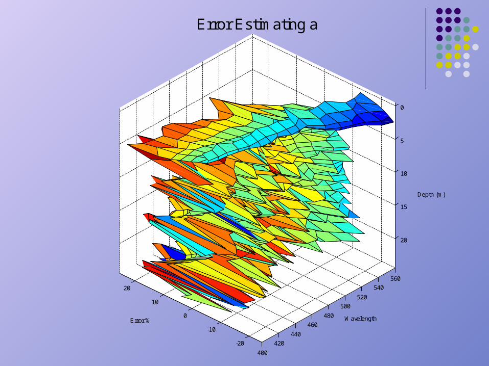
Error Estimating a

Error %

400

450

500

550

0

5

10

15

20

-500

50100

150200

Depth (m)

Wavelength (nm)

Error Estimating bb

Relative Error %

My Model #2

Hydrolight Case 2 IOPs

AC-9 from 9 July 2004 Ocean Optics cruise Cruise 2, Profile 063, ~27 m bottom bb/b = 0.019 (bb from Wetlabs ECOVSF)

Raman scattering only Well mixed water, [Chl] ~3.5 ug/L 50% cloud cover

400 420 440 460 480 500 520 540 5600.05

0.1

0.15

0.2

0.25

0.3

wavelength (nm)

a,c

m-1

a, c: Cruise 2

AOP/IOP Retrieval Results

0.2 0.4 0.6 0.8 1 1.20.2

0.4

0.6

0.8

1

1.2

est

0.05 0.1 0.15 0.2 0.25 0.3

0.05

0.1

0.15

0.2

0.25

0.3

a (m-1)

a est (

m-1

)

0.01 0.02 0.03 0.04 0.05 0.06 0.07

0.01

0.02

0.03

0.04

0.05

0.06

0.07

bb (m-1)

b b,es

t (m

-1)

0 0.05 0.1 0.15 0.2 0.25 0.3 0.35-25

-20

-15

-10

-5

0

a (m-1)

dept

h (m

)

0 0.01 0.02 0.03 0.04 0.05 0.06 0.07 0.08-25

-20

-15

-10

-5

0

bb (m-1)

dept

h (m

)

0 0.2 0.4 0.6 0.8 1 1.2 1.4-25

-20

-15

-10

-5

0

dept

h (m

)

– model

– estimate

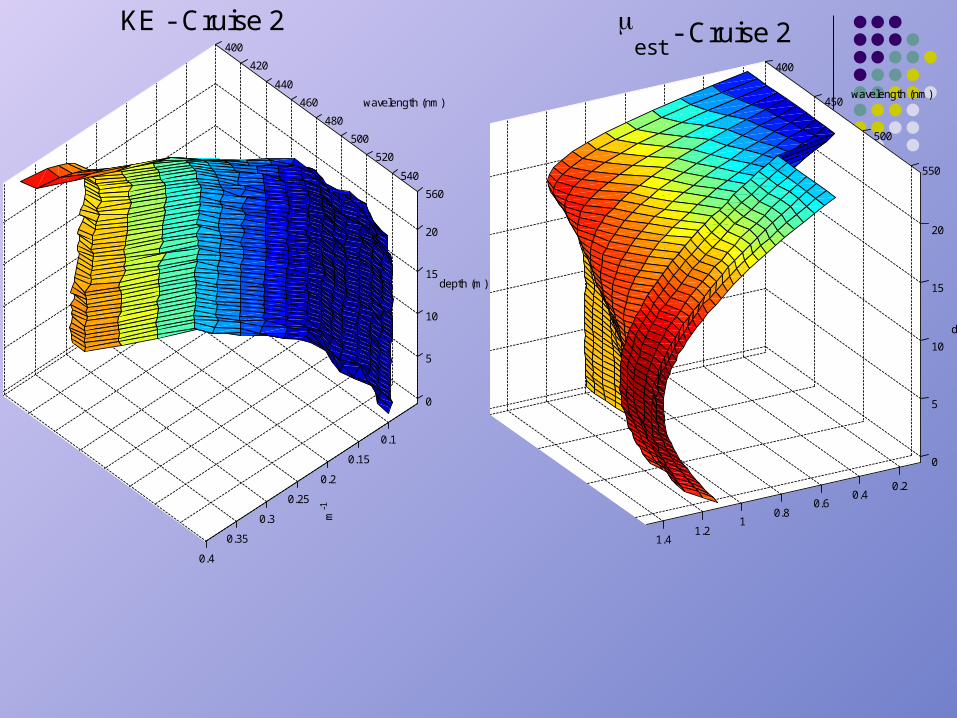
400

420

440

460

480

500

520

540

560

0

5

10

15

20

0.1

0.15

0.2

0.25

0.3

0.35

0.4

depth (m)

wavelength (nm)

m-1

KE - Cruise 2

400

450

500

550

0

5

10

15

20

0.20.4

0.60.8

11.2

1.4

depth (m)

wavelength (nm)

est

- Cruise 2

0 0.01 0.02 0.03 0.04 0.05 0.06 0.07-25

-20

-15

-10

-5

0

RL (sr-1)

dept

h (m

)

400410

420

430440

450

460470

480

490500

510

520530

540

550560

0 0.05 0.1 0.15 0.2 0.25-25

-20

-15

-10

-5

0

R (sr-1)de

pth

(m)

400410

420

430

440450

460

470

480490

500

510520

530

540

550560

Conclusions

Stramska, et al. model is highly tuned to local waters CalCOFI Cruise Petzold Phase Function 15 m limitation is apparent

Requires 3 expensive sensors Absorption is most robust measurement retrieved by

this approach 3-D graphics are useful for visualization of multi-

spectral profile data and error analysis Lots of work to do to theoretical and practical to

advance IOP retrieval from in-water E and L.