INVESTIGATING GEOPHYSICAL SIGNATURES OF LONG TERM

BIODEGRADATION AT THE OIL SPILL SITE IN BEMIDJI, MINNESOTA

by

ASHLEY LAURA

SAMUEL

A Dissertation submitted to

the Graduate School-Newark

Rutgers, The State University of New

Jersey in partial fulfillment of the

requirements

for the degree of

Master of Science

Graduate Program

in

Environmental Geology

written under the direction

of Dr. Lee Slater

and approved by

Newark, New Jersey

October, 2016

©2016

Ashley Laura Samuel

ALL RIGHTS

RESERVED

ii

ABSTRACT OF THE DISSERTATION

Investigating Geophysical Signatures of Long Term Biodegradation at the Oil Spill Site

in Bemidji, Minnesota

By ASHLEY LAURA SAMUEL

Dissertation Director:

Dr. Lee Slater

Biogeophysics is a sub-discipline of geophysics that examines how

microbial interactions with geologic materials affect the geophysical signatures

within the subsurface. Biogeophysical measurements were performed at the

National Crude Oil Spill Fate and Natural Attenuation Research Site in Bemidji,

Minnesota where biodegradation of hydrocarbon contaminants is occurring.

Geophysical measurements were acquired to ascertain whether changes in the pore

fluid conductivity and/or the production of secondary iron minerals such as

magnetite affect geophysical signatures at this site. The effects of hydrology,

geology, oil levels and temperature on geophysical signatures within both an

uncontaminated zone and a biodegraded contaminated zone were investigated.

Resistivity, time domain induced polarization and frequency domain

induced polarization measurements were acquired from a contaminated location

and an uncontaminated location at the site. Results of this study suggests that the

changes in the pore fluid conductivity primarily control the geophysical signatures

when compared to the effects of the formation of magnetite within the smear zone

iii

in the contaminated zone. Hydrology, oil levels and temperature do not appear to

explain the geophysical signatures from the contaminated location, although natural

water table variations can explain the resistivity variations at the uncontaminated

location. This study demonstrates that geophysical methods can be used to assist

in the monitoring of the long term changes in geophysical signatures due to natural

attenuation processes associated with biodegradation of a crude oil spill.

iv

Acknowledgements

This research was based on work supported by the National Science Foundation

Graduate Research Fellowship Program under Grant No. DGE-1313667. First, I

would like to thank my advisor, Lee Slater, and the members of my Advisory

Committee Dimitrios Ntarliagiannis and Kristina Keating. Many thanks to Judy

Robinson, for writing the Matlab script and for her instruction and input. Thanks

also to Kisa Mwakanamale (formerly at Rutgers-Newark), Neil Terry and Pauline

Kessouri of Rutgers-Newark University for their instruction and input. Special

thanks to the other students in the lab, including Sundeep Sharma, Samuel Falzone,

Chi Zhang, Sina Saneiyan and Tonian Robinson, I could not have made it through

this without their advice, encouragement and camaraderie. I also extend my

gratitude to Liz Morrin for her exceptional and undying commitment to

administrative efficiency. I would also like to thank the faculty, staff, and students

of the Earth and Environmental Science Department at Rutgers-Newark for their

constant advice, support, and friendliness. I would also like to thank Andrew Binley

of Lancaster University, England for use of the R3t and cR3t inversion programs that

he developed. I extend my gratitude to the USGS personnel for their field support in

Bemidji, MN as part of the USGS Toxic Hydrology Research Program.

Additionally, I would like to thank Chevron Energy Corporation for funding this

research. Finally, I would like to thank the National Science Foundation Graduate

Research Fellowship Program for funding my education and research.

v

Table of Contents

Abstract i

Acknowledgements iii

Table of Contents iv

iv List of Tables vii

List of Illustrations viii

Introduction 1

Biogeophysics 2

Summary of Research and Significance 2

Biodegradation at Bemidji 3

Linking Geophysical Signatures to Biodegradation 5

Previous Geophysical Applications to Monitoring

Biodegradation

6

Background and Theory 8

Electrical Resistivity 8

Time Domain and Frequency Domain Induced Polarization 10

Petrophysics 12

Petrophysical Properties and Archie’s Law 13

Magnetic Susceptibility 18

Site Description 19

Site History 19

Magnetite at Bemidji 21

Site Geology 22

Site Hydrogeology and Groundwater Temperature Variations 23

vi

Magnetic Susceptibility Field Measurements 25

Specific Conductance 26

Methods 27

Field Electrical Resistivity Measurements 27

Electrical Resistivity Data Processing 30

Electrical Resistivity Data Error Analysis 30

Phase Data Processing 33

Mesh Generation

34

Resistivity Inversion and Visualization 36

Phase Inversion and Visualization

39

Ratio Resistivity Inversions 39

Laboratory Methods

42

SIP Measurements on Sample Filled Laboratory Columns 42

Laboratory SIP Data Processing

SIP Measurements on Sample Filled Laboratory Columns SIP

Measurements on Sample Filled Laboratory Columns

48

Laboratory Magnetic Susceptibility Measurements

50

Sample Porosity Calculations 51

Results

Results

52

Geological Grain Size Analysis 52

Raw Apparent Conductivity and Specific Conductance

Data

54

1-D Radial Resistivity Inversions 55

1-D Radial Ratio Resistivity Inversions 57

Phase Data Processing 59

SIP Laboratory Results 60

vii

Discussion 60

Geological Site Conditions and Geophysical Signatures 60

Magnetic Susceptibility and Geophysical Signatures 61

Hydrology and Geophysical Signatures

62

Magnetic Susceptibility Field and Laboratory Results 64

Laboratory SIP Results 65

Solid Phase Changes and Geophysical Signatures 66

Aqueous Phase Changes and Geophysical Signatures 67

Future Research Considerations 67

Conclusions 68

References 70

Appendices 74

viii

Table 1

List of Tables

Welch’s t-test Geologic Grain Size Statistical Analysis

54

ix

List of Illustrations

Figure 1 Biodegradation Processes and Effects on Geophysical Signatures. 5

Figure 2 Spectral Induced Polarization (SIP) phase shift and TDIP Concept

Diagram. 10

Figure 3 USGS Northwestern Minnesota Topographic Map. 23

Figure 4 Water Level Data. 24

Figure 5 Precipitation Data 24

Figure 6 Magnetic Susceptibility Field Data. 26

Figure 7 Specific conductance contour plot. 27

Figure 8 Vertical Electrical Resistivity Arrays. 28

Figure 9 Site Map with Contaminated and Uncontaminated Regions. 29

Figure 10 Example of Resistance Error Model. 32

Figure 11 Phase Error Models. 34

Figure 12 Tetrahedral mesh. 35

Figure 13 Radial Resistivity Schematic. 38

Figure 14 PSIP Laboratory Column Setup

44

Figure 15 Laboratory Column Experiments Objectives Flowchart. 44

Figure 16 Magnetic Susceptibility Core Reader. 51

Figure 17 Apparent conductivity, specific conductance and water table vs.

elevation.

54

Figure 18 1-D Radial Resistivity Inversions. 56

Figure 19 Uncontaminated 1-D Radial Ratio Resistivity Inversions. 58

Figure 20 Contaminated 1-D Radial Ratio Resistivity Inversions. 59

Figure 21 SIP Laboratory Results. 61

Figure A-1 Phase Inversion Attempt Contaminated. 74

x

Figure A-2 Phase Inversion Attempt Uncontaminated. 75

1

1. INTRODUCTION

Biogeophysics is being used at Bemidji, MN as a method of monitoring long

term natural attenuation. Natural attenuation is defined as the natural processes,

such as biodegradation of contaminants, that remediate the soils and groundwater at

a contaminated site. The aim of this study is to determine the factors that influence

geophysical signatures consistent with natural attenuation at the oil spill site in

Bemidji, MN. The factors that come under scrutiny include: grain size distribution,

hydrology, pore fluid conductivity, magnetite content, magnetic susceptibility, oil

levels and ground water temperatures. Field investigations together with

laboratory experiments will aim to determine which of these factors contribute

substantially to the overall changes in geophysical signatures.

Grain size distribution will be analyzed and compared via a statistical analysis

between the uncontaminated zone and the contaminated zones at Bemidji, MN.

This is to rule out major differences in basic grain size distribution and geology

between the uncontaminated and contaminated regions. Next, the hydrology will

be explored by comparing the precipitation data and water level data at the site.

The specific conductance, or the pore fluid conductivity will be studied by

analyzing field data and setting up a series of laboratory experiments which will

determine how substantially it contributes to the geophysical signatures. In this

same set of laboratory experiments, magnetite will be added to the uncontaminated

sediment samples in amounts double the maximum concentration naturally

occurring in the field, in order to isolate the SIP response to just the magnetite

itself. Magnetic susceptibility will be investigated in order to gauge the presence of

2

iron minerals in both the field and laboratory settings. Finally, oil levels and

temperature variations will be studied to determine whether they contribute to

changes in geophysical signatures.

Biogeophysics

Over time the microbes at Bemidji, MN are breaking down the hydrocarbons

and developing various byproducts via a process called biodegradation.

Geophysical signatures within a contaminant plume where biodegradation has taken

place are associated with lower resistivities when compared with areas without

contamination (Atekwana, et al., 2009). Through the biodegradation process,

microbes are consuming the crude oil and are producing biomass, metabolic

byproduct and microbial remediated processes which in turn can increase the

electrolytic conductivities of the pore fluid (Atekwana, et al., 2009).

By utilizing geophysical field and laboratory methods, we aim to examine the

resistivity, time domain induced polarization and frequency domain induced

polarization response from both a contaminated and an uncontaminated location in

Bemidji, Minnesota. This should demonstrate that geophysical methods can be

used to monitor the long term changes in geophysical signatures.

Summary of Research and Significance

The contaminated area in Bemidji, MN is referred to as The National Crude Oil

Spill Fate and Natural Attenuation Research Site, and is a natural laboratory for the

investigation of biophysicochemical processes associated with the intrinsic

bioremediation of a crude oil spill (Cozzarelli et al., 2001; Eganhouse et al., 1993).

3

The objectives of this study were to demonstrate how field scale geophysical

methods such as resistivity and time domain induced polarization can be used to

compare differences in geophysical signatures between the uncontaminated and

contaminated regions at the oil spill site in Bemidji over time. Geophysical

signatures can also serve as proxy sensors of biodegradation processes. The effects

of any differences in grain size distribution, hydrology, pore fluid conductivity,

magnetite content, magnetic susceptibility, oil levels and ground water temperatures

at the field site on acquired geophysical signatures were also considered.

Furthermore, this study aimed to conduct supporting laboratory frequency

domain induced polarization experiments on Bemidji sediment samples taken from

the uncontaminated region and mixed with magnetite to explore the effects of the

addition of magnetite and pore fluid conductivity on geophysical signatures.

Goethite and siderite were not considered because they do not emit as strong a

magnetic susceptibility signal as magnetite. Additionally, laboratory magnetic

susceptibility measurements and soil porosity measurements were obtained in order

to determine the major contributing factors to changes in geophysical signatures.

This research study involved geophysical signatures from the oil spill site in

Bemidji, MN which were then analyzed at the field scale and in a laboratory setting

concurrently. The geophysical signatures between the field contaminated zone

were compared to the uncontaminated zone, and the effects of grain size

distribution (soil texture) and water table levels were explored. Laboratory SIP

(Spectral Induced Polarization) experiments were performed in order to examine

the effects of pore fluid conductivity and the addition of magnetite.

4

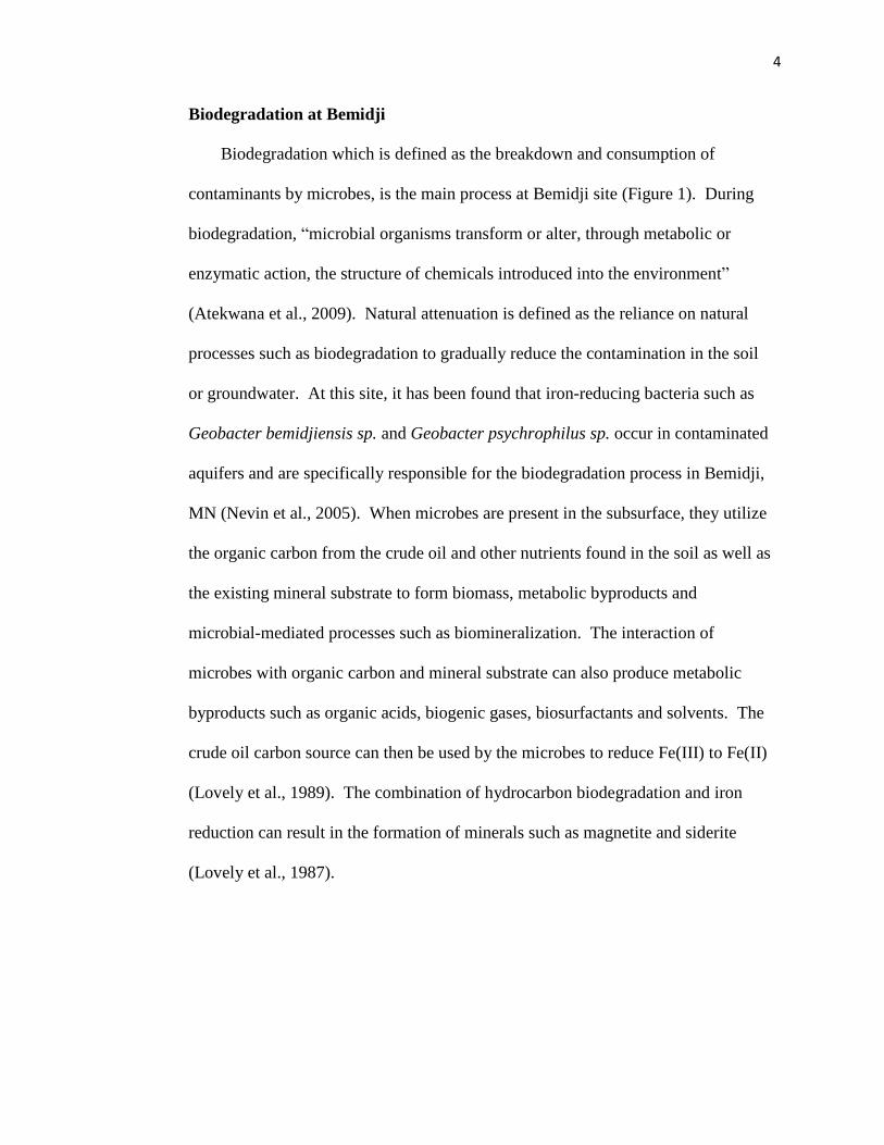
Biodegradation at Bemidji

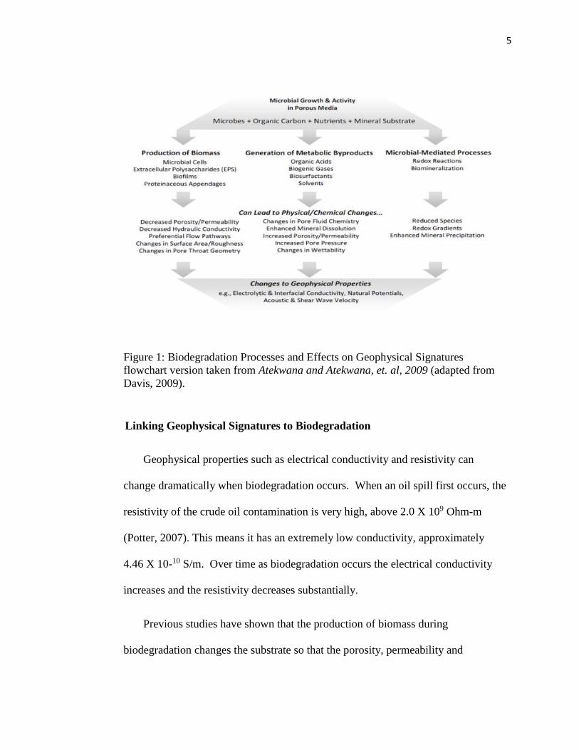
Biodegradation which is defined as the breakdown and consumption of

contaminants by microbes, is the main process at Bemidji site (Figure 1). During

biodegradation, “microbial organisms transform or alter, through metabolic or

enzymatic action, the structure of chemicals introduced into the environment”

(Atekwana et al., 2009). Natural attenuation is defined as the reliance on natural

processes such as biodegradation to gradually reduce the contamination in the soil

or groundwater. At this site, it has been found that iron-reducing bacteria such as

Geobacter bemidjiensis sp. and Geobacter psychrophilus sp. occur in contaminated

aquifers and are specifically responsible for the biodegradation process in Bemidji,

MN (Nevin et al., 2005). When microbes are present in the subsurface, they utilize

the organic carbon from the crude oil and other nutrients found in the soil as well as

the existing mineral substrate to form biomass, metabolic byproducts and

microbial-mediated processes such as biomineralization. The interaction of

microbes with organic carbon and mineral substrate can also produce metabolic

byproducts such as organic acids, biogenic gases, biosurfactants and solvents. The

crude oil carbon source can then be used by the microbes to reduce Fe(III) to Fe(II)

(Lovely et al., 1989). The combination of hydrocarbon biodegradation and iron

reduction can result in the formation of minerals such as magnetite and siderite

(Lovely et al., 1987).

5

Figure 1: Biodegradation Processes and Effects on Geophysical Signatures

flowchart version taken from Atekwana and Atekwana, et. al, 2009 (adapted from

Davis, 2009).

Linking Geophysical Signatures to Biodegradation

Geophysical properties such as electrical conductivity and resistivity can

change dramatically when biodegradation occurs. When an oil spill first occurs, the

resistivity of the crude oil contamination is very high, above 2.0 X 109 Ohm-m

(Potter, 2007). This means it has an extremely low conductivity, approximately

4.46 X 10-10 S/m. Over time as biodegradation occurs the electrical conductivity

increases and the resistivity decreases substantially.

Previous studies have shown that the production of biomass during

biodegradation changes the substrate so that the porosity, permeability and

6

hydraulic conductivity decrease (e.g., Taylor et al., 1990; Cunningham et al., 1991;

Vandevivere and Baveye, 1992; Baveye et al., 1998; Seifert and Engesgaard, 2007;

Brovelli et al., 2009). This creates preferential flow pathways and changes the

surface area, roughness and pore throat geometry of the subsurface (e.g., Seifert,

2005; Brovelli et al., 2009). The formation of metabolic byproducts can lead to

physical and chemical changes such as changes in pore fluid chemistry, enhanced

mineral dissolution, increased porosity, permeability and pore pressure and changes

in wettability (e.g., Abdel Aal et al., 2004; Atekwana et al., 2004a, 2004b, 2004c,

Atekwana et al., 2009).

Natural attenuation occurs when biodegradation and natural hydraulic

processes are allowed to happen naturally and without human intervention.

Biogeophysics provides an alternative method for monitoring natural attenuation by

studying changes in geophysical signatures. The most important mechanisms

relevant to this study are the well-established biogeophysical signatures related to

changes in electrolytic conductivity due to solid and aqueous phase processes

accompanying biodegradation (Atekwana, et. al, 2009). The combination of redox

reactions and biomineralization occurring simultaneously during biodegradation

leads to reduced species, redox gradients and enhanced mineral precipitation. All

of these processes including: production of biomass, generation of metabolic

byproducts and microbial-mediated processes can potentially lead to changes in

geophysical properties such as electrolytic and interfacial conductivities (Atekwana,

et. al, 2009).

Previous Geophysical Applications to Monitoring Biodegradation

7

Prior studies have used field scale geophysical techniques including resistivity

and conductivity (Allen, et al., 2007) and magnetic susceptibility (Atekwana, et. al,

2014) to monitor biodegradation at hydrocarbon contaminated sites. Allen, et. al.

(2007) showed that the presence of, “microbial populations, including the various

hydrocarbon-degrading, syntrophic, sulfate-reducing, and dissimilatory-iron-

reducing populations, was a contributing factor to the elevated conductivity

measurements.”

Magnetic susceptibility has been proven to play an important role in

identifying zones where microbial-mediated iron reduction is occurring. Within the

uncontaminated zone, the area where the water table is fluctuating is known as the

water table fluctuation zone. However, in the contaminated region, this area is

known as the smear zone because the contaminant is smeared within the fluctuating

water table. Atekwana, et al., 2014 observed that magnetic susceptibility values are

highest within the smear zone and are also coincident with high concentrations of

dissolved Fe(II) and organic carbon content, suggesting that the smear zone is most

biologically active.

Laboratory studies have also been performed on sediment samples taken from

the research site in Bemidji, Minnesota utilizing frequency domain induced

polarization and magnetic susceptibility; specifically, the study performed by

Mewafy, et al. (2013) to show the effect of the presence of an amount of magnetite

equivalent to that naturally occurring at Bemidji, MN on geophysical signatures.

They performed laboratory experiments using magnetite in a matrix of pure sand

and saturated the columns using an NaCl solution with conductivity similar to the

8

actual uncontaminated Bemidji conductivity. Their goal was to observe the effect

of adding magnetite due to biodegradation on geophysical signatures. They

observed a clear increase in the imaginary conductivity response with increasing

magnetite content. Their experiment differs from this study in that we used double

the amount of the maximum concentration of magnetite found at Bemidji in our

column experiments in order to isolate and magnify the effect of the magnetite on

the SIP signatures.

Mewafy, et al, (2013) also used actual contaminated Bemidji cores and

uncontaminated cores and saturated them with NaCl solution with pore fluid

conductivity similar to the actual contaminated Bemidji pore fluid conductivity and

uncontaminated pore fluid conductivity, respectively. Samples from the

contaminated region were found to have higher conductivity values than those from

the uncontaminated region (Mewafy, et. al, 2013).

In addition, Abdel Aal, et. al, (2014) used an agar gel with conductivity similar

to the conductivity of the uncontaminated zone at Bemidji for three different iron

minerals to study the effect of mineralization on geophysical signatures. Their

results indicated that the quadrature conductivity magnitude increased with

decreasing grain size diameter of magnetite and pyrite with a progressive shift of

the characteristic relaxation peak toward higher frequencies. The quadrature

conductivity response of a mixture of different grain sizes of iron minerals was

shown to be additive, whereas magnetic susceptibility measurements were

insensitive to the variation in grain size diameters (1– 0.075mm) (Abdel Aal et. al,

2014). For our study we only used a magnetite grain size of 106mm and studied the

9

phase response, quadrature conductivity (or imaginary conductivity), real

conductivity, resistivity and magnetic susceptibility of the samples.

2. BACKGROUND AND THEORY

Electrical Resistivity

Electrical Resistivity is a low frequency direct current (DC) geophysical

technique for imaging sub-surface structures from electrical resistivity

measurements made via electrodes arranged horizontally at the surface, or by

electrodes arranged vertically in a borehole configuration. A commonly used

electrode measurement configuration due to its higher signal to noise ratio is the

Wenner array.

For a Wenner configuration current is injected across two current electrodes A

and B, and the potential is measured between two potential electrodes M and N.

For a Wenner configuration the order of electrodes is A, M, N and B. Ohm’s Law

allows the resistance, R, to be calculated by dividing the voltage, V, by the current,

I (Equations 1).

V = IR (1)

The calculated resistances can then be used to approximate the apparent

resistivity, ρa, (Equation 2) which is the equivalent resistivity assuming 3D current

flow through a homogeneous half space (surface of the) earth:

10

∆V

I= R =

ρa

2π[

1

AM−

1

MB−

1

AN+

1

NB ] (2)

Inverse methods are used to determine a model of the subsurface resistivity

structure by minimizing the differences between field observations of apparent

resistivity and the apparent resistivities determined from a numerical forward model

solution for a particular resistivity model.

Time Domain and Frequency Domain Induced Polarization

The measured time domain induced polarization (TDIP) response indicates the

ability of a ground material to polarize at its interfaces. Lithology and fluid

conductivity determine the induced polarization (IP) response of rocks and soils

within the subsurface. IP measurements are sensitive to the low-frequency

capacitive properties of rocks and soils, which are controlled by diffusion

polarization mechanisms operating at the grain-fluid interface. Induced polarization

additionally measures the degree of electrical charge stored in the electrical double

layer, forming at mineral-fluid interfaces in porous media (Mwakanyamale, et. al,

2012). IP interpretation typically is in terms of the conventional field IP

parameters: chargeability and phase angle. These parameters are dependent upon

both surface polarization mechanisms and bulk (volumetric) conduction

mechanisms (Slater and Lesmes, 2002).

11

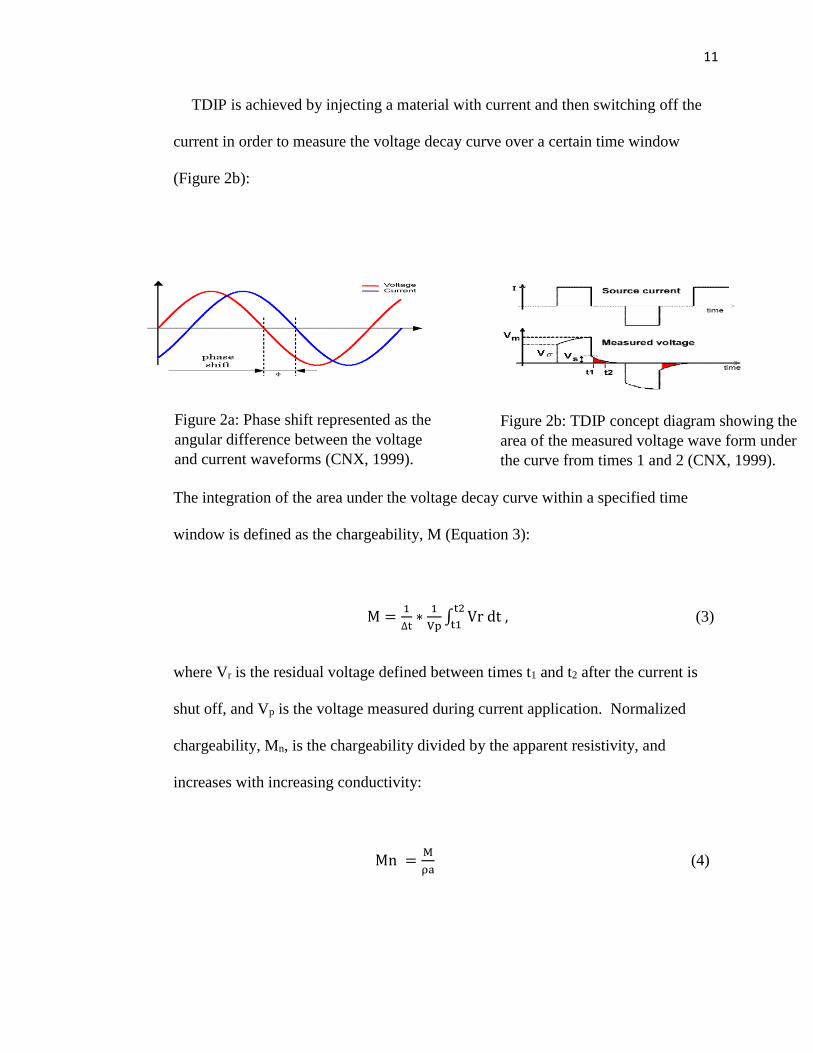
TDIP is achieved by injecting a material with current and then switching off the

current in order to measure the voltage decay curve over a certain time window

(Figure 2b):

The integration of the area under the voltage decay curve within a specified time

window is defined as the chargeability, M (Equation 3):

M =1

∆t∗

1

Vp∫ Vr dt

t2

t1 , (3)

where Vr is the residual voltage defined between times t1 and t2 after the current is

shut off, and Vp is the voltage measured during current application. Normalized

chargeability, Mn, is the chargeability divided by the apparent resistivity, and

increases with increasing conductivity:

Mn =M

ρa (4)

Figure 2a: Phase shift represented as the

angular difference between the voltage

and current waveforms (CNX, 1999).

Figure 2b: TDIP concept diagram showing the

area of the measured voltage wave form under

the curve from times 1 and 2 (CNX, 1999).

12

The normalized chargeability quantifies the magnitude of surface polarization

(Slater and Lesmes, 2002). The angle which represents the degree to which the

voltage waveform lags behind the current waveform is known as the phase shift ()

(Figure 2a).

Phase angles have been found to be empirically related through laboratory

experiments to the chargeabilities by multiplying the chargeability by a factor of 1.3

to obtain the phase (Mwakanyamale, et. al, 2012). The phase angle and

conductivity magnitude can also be used to calculate both the real (’) and

imaginary (”) parts of complex conductivity (Equations 5 & 6).

The frequency domain induced polarization effect or the spectral induced

polarization (SIP) effect is similar to the TDIP effect however it measures the

resistances over a spectrum of frequencies as opposed to time. SIP measures the

resistances, phase angles and frequency spectrum which can then be used to

determine the resistivities along with the real and imaginary conductivities, in the

same manner as in TDIP.

SIP can be converted to TDIP, via the Fourier Transform. The Fourier

transform decomposes a function of time (a signal) into the frequencies that make it

up, and therefore allows TDIP to be converted to SIP (Huang, 1993).

Complex Conductivity Measurements

The complex conductivity is given by:

σ∗ = |σ| exp(i) = σ′ + iσ" , (5)

13

|σ| = ((σ′)2 + (σ")2)1/2 . (6)

where * is the complex conductivity, composed of a real component, ’, and an

imaginary component, ’’, i is equivalent to √−1 , || is the magnitude and is the

phase lag (Mooney, 2013). The magnitude of the complex conductivity is given by

Equation 6, where ’ is much greater than ”, and therefore the magnitude of the

complex conductivity essentially reflects the real component of the conductivity.

The imaginary part σ” is mostly related to the counter-ion content at the grain and

fracture boundaries. The imaginary part (and phase) increases with higher fracture

density and with smaller fractures and pores, due to the increase in the overall

mineral surface area. If air voids are present, real and imaginary conductivities

decrease substantially. However, in fluid filled pores, the real part increases

significantly while the imaginary part decreases significantly with increasing water

content (Mooney, 2013). The phase, can be determined from:

’ = || ∗ cos() (7)

” = || ∗ sin() (8)

The imaginary part of the conductivity, ”, is related to the phase, by Equations 7

& 8, where the phase lag is the angle which represents the degree to which the

voltage waveform lags behind the current waveform and is also known as the phase

shift () (Figure 2a).

14

The phase captures the influence of the imaginary part and depends both on

electromigration (conduction) properties (through σ ') and charge storage (through σ

") (Mooney, 2013). The phase angle can be used to calculate both the real (’) and

imaginary (”) parts of the complex conductivity.

Petrophysical Properties and Archie’s Law

Geophysical signatures are related to the physical properties of the geologic

material. Archie’s Law is an empirical quantitative relationship between porosity,

electrical conductivity, and brine saturation of rocks (Archie, 1942). In the case

where there is only electrolytic conduction, or conduction through the pore fluid,

the relationships between the physical properties of the geologic material and the

geophysical signatures are given by the following equation (Equation 9):

F = L

C

φint=

τ

φint , (9)

where the formation factor, F, is a geophysical property which can be expressed as

the ratio of the tortuosity, to the interconnected porosity, int (Equation 9).

Tortuosity is a measure of how tortuous or how much the path through the

interconnected pore spaces deviates from the direct linear distance between two

points within a certain geologic material. The tortuosity is the ratio between the

total length of the tortuous path, L and the direct linear distance, C between any two

points (Equation 9). The interconnected porosity or the effective porosity, int,

15

represents the porosity of a rock or sediment available to contribute to fluid flow

through the rock or sediment. The interconnected porosity can be calculated by

subtracting the clay bound water (CBW) or the volume of water that remains bound

to the surfaces of certain hydrophilic mineral grains and therefore does not

contribute to fluid flow, from the total porosity (Equation 10).

φint = φ − CBW (10)

The total porosity, φ, is expressed as the ratio of the total volume of voids (volume

of air and volume of water) over the total volume of solids and voids (Equation 11).

φ = Va+Vw

Vt=

Vv

Vt (11)

Alternatively, the formation factor can also be written as the ratio between earth and

w, where earth is the overall resistivity of the geologic material (which is simply

the inverse of the electrical conductivity of the geologic material or 1/earth) and w

is the resistivity of the pore fluid or the brine resistivity (Equation 12).

F = ρearth

ρw=

σw

σearth

(12)

Electrical resistivity, is an intrinsic property that quantifies how strongly a

given material opposes the flow of electric current. A low resistivity indicates a

material that readily allows the movement of electric charge. The general term for

16

the resistivity, , is equal to the reciprocal of the general term for the electrical

conductivity, , which is a measure of the ability of a material to conduct electrical

current. Furthermore, the conductivity of the fluid within the soil or rock dominates

σ’(electrolytic conductivity) if the geologic material is saturated and has reasonable

porosity. Therefore, conductivity increases with increasing porosity and water

content (Archie, 1942). Due to the inverse relationship between the electrical

resistivity and the electrical conductivity, the apparent formation factor can also be

rewritten as the ratio of w to the earth, where w is the pore fluid conductivity, also

known as the brine conductivity or salinity, and earth is the overall conductivity of

the geologic material (Equation 12).

In rocks with conductive minerals, there is a more complex dependence of the

formation factor on w, temperature and the type of ions in solution. In these

instances, the formation factor is referred to as the apparent formation factor. The

apparent formation factor has been shown to be independent of the w, (or 1/w)

only for a certain class of petrophysically simple rocks (Schlumberger Oil Field

Glossary, 2016). Therefore, the apparent formation factor is solely a function of

pore geometry and describes how much more resistive the porous rock is relative to

the fluid filling pores.

In Archie’s Law, the interconnected porosity is raised to a cementation exponent,

m, which models the degree of connectivity of the pores and is thus related to

tortuosity and how much ‘cementation’ has occurred in the pores. If the pore

network were to be modelled as a set of parallel capillary tubes, a cross-sectional

area average of the rock's resistivity would yield porosity dependence equivalent to

17

a cementation exponent of 1 (Glover, 2012). However, the tortuosity if the rock

increases the cementation exponent to a number higher than 1 and less than 5

(Glover, 2012). This relates the cementation exponent to the permeability of the

rock, or the ability of a geologic material to allow liquids to pass through it.

Increasing permeability decreases the cementation exponent.

Saturation, Sw, is the ratio of the volume of water, Vw to the volume of voids, Vv

(Equation 13).

Sw = Vw

Va+Vw=

Vw

Vv (13)

When the Sw is raised to a saturation exponent, n, it can be expressed as the

ratioearth to the sat, where sat is the resistivity of the geologic material when it is

fully saturated (Equation 14). Similarly, the Swn can also be expressed as the ratio

of the earth to the sat, where sat is the conductivity of the geologic material when

fully saturated (Equation 14) (Archie, 1942).

Swn =

ρearth

ρsat=

σearth

σsat

(14)

The saturation exponent, n, models the dependency on the presence of non-

conductive fluid (such as hydrocarbons) in the pore-space, and is related to the

wettability of the rock, or the tendency of one fluid to spread on, or adhere to, a

solid surface in the presence of other immiscible fluids (Glover, 2012). The higher

18

the wettability of geologic materials, even for low water saturation values, the more

likely that a continuous film along the pore walls is maintained, making the

geologic material conductive along the surface of its constituent minerals

(Abdallah, 2007).

Assuming only electrolytic conduction, all of these aforementioned physical

properties of geologic materials, including the interconnected porosity and

saturation, are empirically related to their geophysical signatures such as the

electrical conductivity of the pore fluid and the overall conductivity of the geologic

material through Archie’s Law (Equation 15). Archie’s law, which applies when it

relates the bulk conductivity to the conductivity of a pore fluid.

σearth = 1

ρearth=

σw

F= ( σw)(φint

m )(Swn ) (15)

However, there are other conduction paths available to electrical current

including conduction along the surfaces of mineral grains and through the mineral

grain itself. Archie’s Law can be modified to include surface conduction (Equation

16) in the following equation:

σearth = 1

ρearth=

σw

F+ σsurf , (16)

where surf is electrical conductivity along the surface of the mineral grains.

Surface conduction along mineral grains is due to the existence of the electrical

double layer (EDL) which acts as a conduit for electrical current.

19

The EDL is a distribution of charges that is on the surface of the mineral grain as

a result of the fluid. It consists of a structure of negatively charged mineral grain

adjacent to a mixture of positive and negative charges that develop in response to

the negatively charged mineral grain. The EDL contains three parallel layers of

charge surrounding the mineral grain. The first layer, also known as the Stern

Layer, is associated with the fluid itself comprised of negative ions adsorbed onto

the object due to chemical interactions. The second layer is composed of positive

and negative ions attracted to the surface charge via the coulomb force, electrically

screening the first layer. This third layer, also known as the diffuse layer, is loosely

associated with the mineral grain because it is made of free ions that move in the

fluid under the influence of electrical attraction and thermal motion rather than

being firmly anchored (Bard, 1980). As temperature increases, the electrical

conductivity through the EDL also increases.

Magnetic Susceptibility

Magnetic susceptibility is the ability of a material to become magnetized, and

indicates whether a material is attracted into or repelled out of a magnetic field.

Quantitative measures of the magnetic susceptibility also provide insights into the

structure of materials, such as bonding and energy levels.

The principle of operation of the probe (Operating manual, Bartington

Instruments) is based on the magnetic state of a specimen, which is generally

described by the following equation:

20

B = μ0(H + M)

(17)

where B is the flux density of the specimen in Tesla, μo is the permeability of free

space equal to a constant (4π × 10−7), H is the applied field strength in AT/m and M

is the magnetization of the specimen in Tesla. Dividing through by H, we get:

μr = μ0 + μ0k

(18)

where μr is the relative permeability of the specimen (dimensionless) and κ is the

magnetic susceptibility of the specimen (dimensionless). Rearranging, we get:

μ0k = μr − μ0 (19)

Magnetite is an iron rich mineral with chemical formula Fe3O4, and it is

ferrimagnetic. Ferrimagnetic mineral precipitates such as magnetite will have a

much higher magnetic susceptibility (MS) signal than other minerals which are not

magnetic. Magnetite is important because its presence signifies the precipitation of

iron minerals due to biodegradation. Therefore, MS measurements are a useful

technique for determining the presence of ferrimagnetic minerals.

3. SITE DESCRIPTION

Site History

21

In August 1979, a high pressure crude oil pipeline burst just northwest of the

town of Bemidji, Minnesota, spilling 1,700,000 L of crude oil onto the ground

surface, contaminating the underlying shallow outwash aquifer (Figure 4). The

contaminated region covered an area of 6500 m2. Cleanup efforts were made in

1980, after which about 24% (or 400,000 L) of the crude oil remained infiltrated

throughout the subsurface in the unsaturated zone and around the water table

(USGS Fact Sheet 084-98, 1998). This crude oil spill continues to be a source of

contaminants to a shallow outwash aquifer. The oil is moving as a separate fluid

phase, as dissolved petroleum constituents in ground water, and as vapors in the

unsaturated zone.

The contaminated area in Bemidji, MN is referred to as The National Crude

Oil Spill Fate and Natural Attenuation Research Site, and is a natural laboratory for

the investigation of biophysicochemical processes associated with the intrinsic

bioremediation of a crude oil spill. The smear zone, the area located below and

above the water table, was found to have predominantly residual and free phase

hydrocarbon. The biodegradation of the toxic chemicals leaching from the crude

oil by microbial populations within the smear zone is our target area of interest

(Cozzarelli et al., 2001; Eganhouse et al., 1993).

USGS scientists studying the site found that toxic chemicals leaching from the

crude oil were rapidly degraded by natural microbial populations. Significantly, it

was shown that the plume of contaminated ground water stopped enlarging after a

few years as rates of microbial degradation came into balance with rates of

contaminant leaching. This was the first and best-documented example of intrinsic

22

bioremediation in which naturally occurring microbial processes remediates

contaminated ground water without human intervention (Chapelle, U.S.G.S., Fact

Sheet FS-054-95)

The contaminated area in Bemidji, MN offers a unique opportunity to study the

geophysical signatures of a mature oil spill. The spill history at the site has been

well characterized and monitored by the USGS for the last 37 years.

Magnetite at Bemidji

Magnetite is an important mineral precipitate at Bemidji because it indicates a

certain level of biodegradation occurring within the smear zone. Magnetite is a

black, metallic mineral that can be formed or precipitated either through abiotic

mineralization or biotic mineralization. Abiotic mineralization, or inorganic

mineralization, refers to a process where an inorganic substance precipitates in an

inorganic matrix without the aid of biological organisms (Dupraz, 2009). Chemical

conditions necessary for abiotic magnetite mineral formation develop via

environmental processes, such as evaporation or degassing. Furthermore, the

substrate for mineral deposition is abiotic (i.e. contains no organic compounds).

Abiotic magnetite is a mineral which is formed as part of a variety of igneous rocks,

pegmatites, contact metamorphic rocks and hydrothermal veins. In our modern

Earth, magnetite seldom forms in sedimentary environments. During the Early

Proterozoic Eon (2.5 to 1.6 billion years ago), however, large deposits of magnetite

precipitated directly from seawater, as it was a time when the world’s oceans and

atmosphere had not yet become as oxygen-rich as they are now (University of

Minnesota Geology Department Website, 2016). Bemidji is located in the area that

23

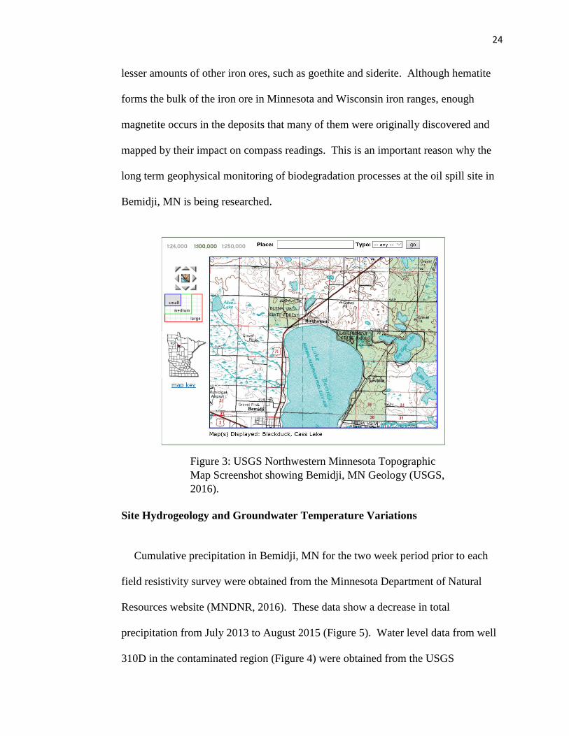
is in the slightly Northwestern part of Minnesota (Figure 3) (Google Maps, 2016).

The iron ranges of Minnesota and Wisconsin once held enormous amounts of

magnetite and hematite, along with lesser amounts of other iron ores, such as

goethite and siderite. Although hematite forms the bulk of the iron ore in Minnesota

and Wisconsin iron ranges, enough magnetite occurs in the deposits that many of

them were originally discovered and mapped by their impact on compass readings.

In biotic mineralization, or biomineralization, native microbes are converting

the petroleum derivatives into carbon dioxide, methane, and other biodegradation

products. During biomineralization, magnetite can be nucleated and grown by

biologically inducing chemical reactions. Magnetite can also be precipitated at a

specific location within or on the cell of a microorganism, by having Fe(III) convert

to Fe(II) which leads to the precipitation of the minerals either by nucleation or

growth, which is controlled by ferrous iron concentration and/or pH (Bazylinkski

and Frankel, 2003).

Site Geology

Geographically, Bemidji, MN is located in the slightly Northwestern part of

Minnesota. The area in which the Bemidji oil contaminated site is located, which

both include and surround glacial lakebeds, include a variety of geologic rock types.

These glacial lakebed areas lie in a vast plain in the bed of Glacial Lake Agassiz,

which extends north and northwest from the Big Stone Moraine (or Iron Range),

beyond Minnesota's borders into Canada and North Dakota (University of

Minnesota Geology Department, 2016 The Big Stone Moraine of Northwestern

Minnesota once held enormous amounts of magnetite and hematite, along with

24

lesser amounts of other iron ores, such as goethite and siderite. Although hematite

forms the bulk of the iron ore in Minnesota and Wisconsin iron ranges, enough

magnetite occurs in the deposits that many of them were originally discovered and

mapped by their impact on compass readings. This is an important reason why the

long term geophysical monitoring of biodegradation processes at the oil spill site in

Bemidji, MN is being researched.

Site Hydrogeology and Groundwater Temperature Variations

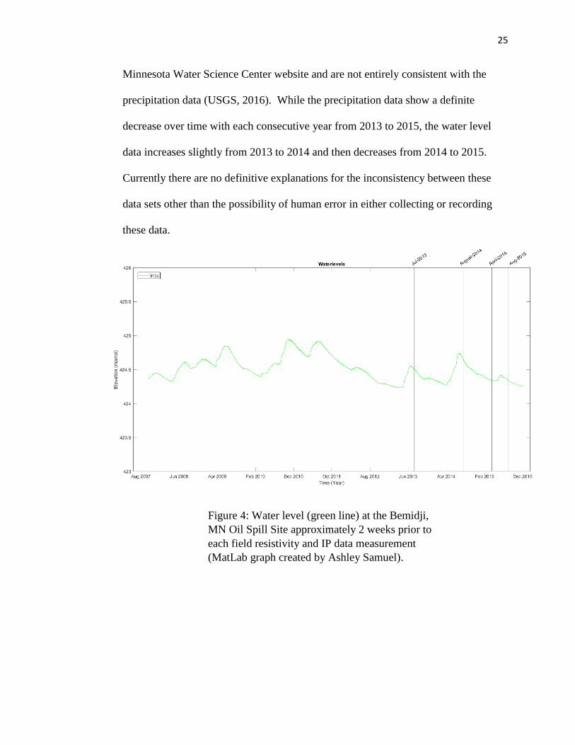
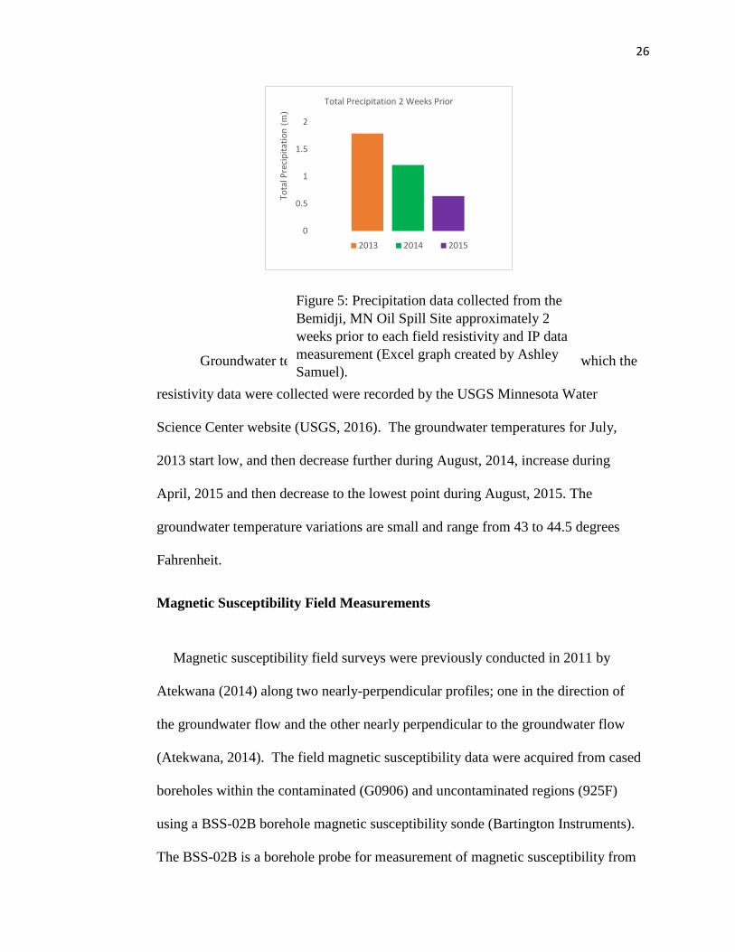
Cumulative precipitation in Bemidji, MN for the two week period prior to each

field resistivity survey were obtained from the Minnesota Department of Natural

Resources website (MNDNR, 2016). These data show a decrease in total

precipitation from July 2013 to August 2015 (Figure 5). Water level data from well

310D in the contaminated region (Figure 4) were obtained from the USGS

Figure 3: USGS Northwestern Minnesota Topographic

Map Screenshot showing Bemidji, MN Geology (USGS,

2016).

25

Minnesota Water Science Center website and are not entirely consistent with the

precipitation data (USGS, 2016). While the precipitation data show a definite

decrease over time with each consecutive year from 2013 to 2015, the water level

data increases slightly from 2013 to 2014 and then decreases from 2014 to 2015.

Currently there are no definitive explanations for the inconsistency between these

data sets other than the possibility of human error in either collecting or recording

these data.

Figure 4: Water level (green line) at the Bemidji,

MN Oil Spill Site approximately 2 weeks prior to

each field resistivity and IP data measurement

(MatLab graph created by Ashley Samuel).

26

Groundwater temperature variations in Bemidji, MN on the dates which the

resistivity data were collected were recorded by the USGS Minnesota Water

Science Center website (USGS, 2016). The groundwater temperatures for July,

2013 start low, and then decrease further during August, 2014, increase during

April, 2015 and then decrease to the lowest point during August, 2015. The

groundwater temperature variations are small and range from 43 to 44.5 degrees

Fahrenheit.

Magnetic Susceptibility Field Measurements

Magnetic susceptibility field surveys were previously conducted in 2011 by

Atekwana (2014) along two nearly-perpendicular profiles; one in the direction of

the groundwater flow and the other nearly perpendicular to the groundwater flow

(Atekwana, 2014). The field magnetic susceptibility data were acquired from cased

boreholes within the contaminated (G0906) and uncontaminated regions (925F)

using a BSS-02B borehole magnetic susceptibility sonde (Bartington Instruments).

The BSS-02B is a borehole probe for measurement of magnetic susceptibility from

0

0.5

1

1.5

2

Tota

l Pre

cip

itat

ion

(m)

Total Precipitation 2 Weeks Prior

2013 2014 2015

Figure 5: Precipitation data collected from the

Bemidji, MN Oil Spill Site approximately 2

weeks prior to each field resistivity and IP data

measurement (Excel graph created by Ashley

Samuel).

27

10-5 to 10-1 centimeter-gram-seconds (cgs) and operates at 1.36 kHz. The magnetic

susceptibility probe is characterized by high vertical and horizontal resolution up to

25 mm, with the region of detection being situated 190 mm from the end of the

borehole (Atekwana, et. al, 2014). This probe identifies areas of microbial

mediated iron reduction, resulting in a high positive response to ferrimagnetic

minerals such as magnetite.

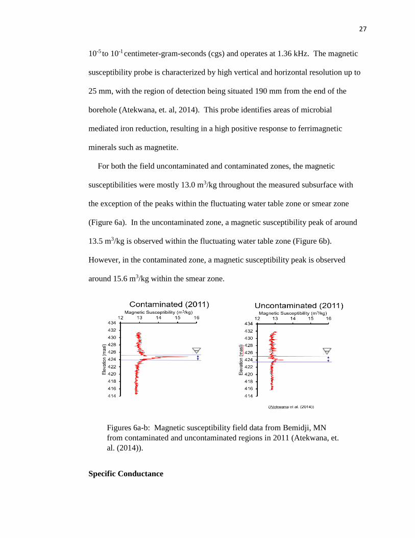
For both the field uncontaminated and contaminated zones, the magnetic

susceptibilities were mostly 13.0 m3/kg throughout the measured subsurface with

the exception of the peaks within the fluctuating water table zone or smear zone

(Figure 6a). In the uncontaminated zone, a magnetic susceptibility peak of around

13.5 m3/kg is observed within the fluctuating water table zone (Figure 6b).

However, in the contaminated zone, a magnetic susceptibility peak is observed

around 15.6 m3/kg within the smear zone.

Specific Conductance

Figures 6a-b: Magnetic susceptibility field data from Bemidji, MN

from contaminated and uncontaminated regions in 2011 (Atekwana, et.

al. (2014)).

28

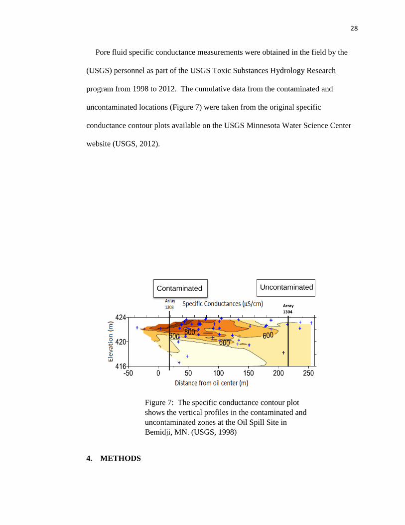
Pore fluid specific conductance measurements were obtained in the field by the

(USGS) personnel as part of the USGS Toxic Substances Hydrology Research

program from 1998 to 2012. The cumulative data from the contaminated and

uncontaminated locations (Figure 7) were taken from the original specific

conductance contour plots available on the USGS Minnesota Water Science Center

website (USGS, 2012).

4. METHODS

Array

1304

Uncontaminated Contaminated

Figure 7: The specific conductance contour plot

shows the vertical profiles in the contaminated and

uncontaminated zones at the Oil Spill Site in

Bemidji, MN. (USGS, 1998)

29

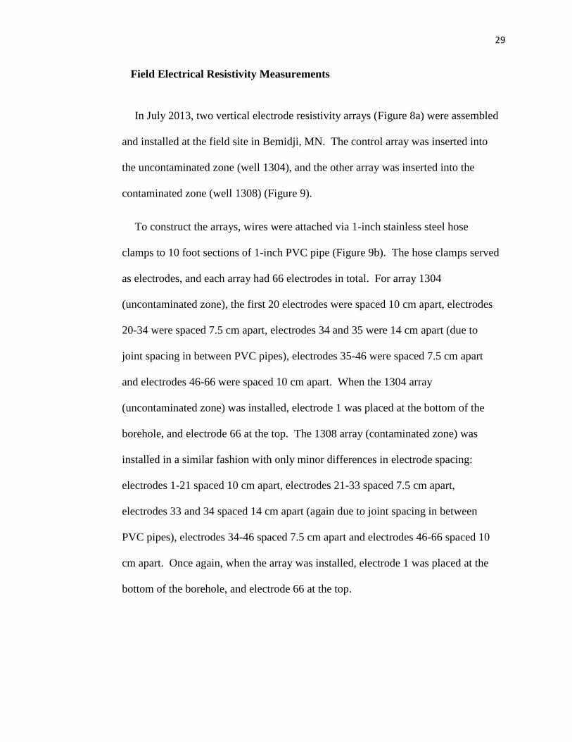
Field Electrical Resistivity Measurements

In July 2013, two vertical electrode resistivity arrays (Figure 8a) were assembled

and installed at the field site in Bemidji, MN. The control array was inserted into

the uncontaminated zone (well 1304), and the other array was inserted into the

contaminated zone (well 1308) (Figure 9).

To construct the arrays, wires were attached via 1-inch stainless steel hose

clamps to 10 foot sections of 1-inch PVC pipe (Figure 9b). The hose clamps served

as electrodes, and each array had 66 electrodes in total. For array 1304

(uncontaminated zone), the first 20 electrodes were spaced 10 cm apart, electrodes

20-34 were spaced 7.5 cm apart, electrodes 34 and 35 were 14 cm apart (due to

joint spacing in between PVC pipes), electrodes 35-46 were spaced 7.5 cm apart

and electrodes 46-66 were spaced 10 cm apart. When the 1304 array

(uncontaminated zone) was installed, electrode 1 was placed at the bottom of the

borehole, and electrode 66 at the top. The 1308 array (contaminated zone) was

installed in a similar fashion with only minor differences in electrode spacing:

electrodes 1-21 spaced 10 cm apart, electrodes 21-33 spaced 7.5 cm apart,

electrodes 33 and 34 spaced 14 cm apart (again due to joint spacing in between

PVC pipes), electrodes 34-46 spaced 7.5 cm apart and electrodes 46-66 spaced 10

cm apart. Once again, when the array was installed, electrode 1 was placed at the

bottom of the borehole, and electrode 66 at the top.

30

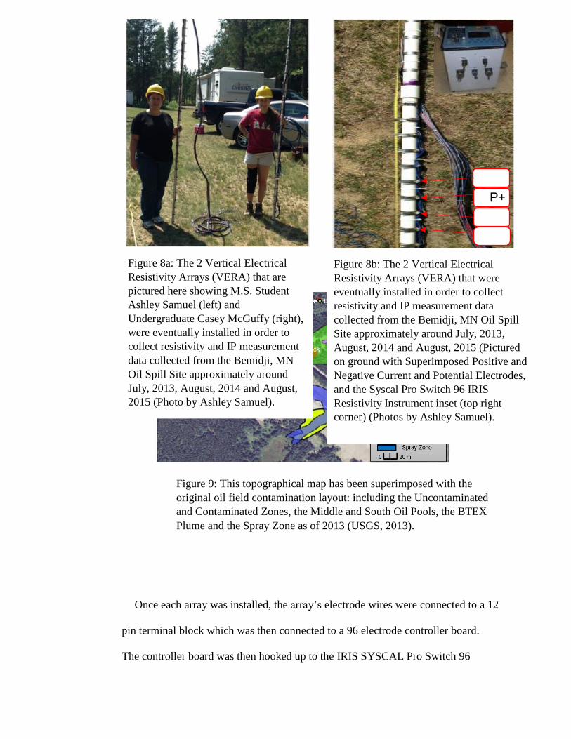
Once each array was installed, the array’s electrode wires were connected to a 12

pin terminal block which was then connected to a 96 electrode controller board.

The controller board was then hooked up to the IRIS SYSCAL Pro Switch 96

P+

Figure 8a: The 2 Vertical Electrical

Resistivity Arrays (VERA) that are

pictured here showing M.S. Student

Ashley Samuel (left) and

Undergraduate Casey McGuffy (right),

were eventually installed in order to

collect resistivity and IP measurement

data collected from the Bemidji, MN

Oil Spill Site approximately around

July, 2013, August, 2014 and August,

2015 (Photo by Ashley Samuel).

Figure 8b: The 2 Vertical Electrical

Resistivity Arrays (VERA) that were

eventually installed in order to collect

resistivity and IP measurement data

collected from the Bemidji, MN Oil Spill

Site approximately around July, 2013,

August, 2014 and August, 2015 (Pictured

on ground with Superimposed Positive and

Negative Current and Potential Electrodes,

and the Syscal Pro Switch 96 IRIS

Resistivity Instrument inset (top right

corner) (Photos by Ashley Samuel).

Figure 9: This topographical map has been superimposed with the

original oil field contamination layout: including the Uncontaminated

and Contaminated Zones, the Middle and South Oil Pools, the BTEX

Plume and the Spray Zone as of 2013 (USGS, 2013).

31

Electrode resistivity and IP instrument. This setup allowed for resistivity and

normalized chargeability measurements to be collected automatically by the IRIS

instrument. The IRIS instrument combines a transmitter, a receiver and a switching

unit and is supplied by a 12V marine battery. The measurements are carried out

automatically using a 50V output voltage, 2.5A current, 250W power and 3 stacks

(number of readings) per resistivity and IP measurement. The Induced Polarization

chargeability (IP) is also measured through 20 windows for a detailed analysis of

the decay curves displayed on the graphic LCD screen (IRIS Instruments Brochure,

2016). The measurements were obtained using a basic Wenner configuration due to

its higher signal to noise ratio. Using both a = 1 and a = 2 electrode spacings,

normal and reciprocal measurements were taken in July 2013, August 2014, April

2015 and August 2015 (Figures 9a-b).

Electrical Resistivity Data Processing

The electrical resistivity data were first processed by performing a thorough

error analysis which eliminated the resistance errors greater than a threshold

percentage between the normal and reciprocal measurements. These processed data

were then inverted using inverse modelling techniques, which use the acquired data

to establish a best fit model for those data using R3t inversion software. The

resulting inverted resistivities, calculated by R3t, were then visualized using the

VisIT software program.

Electrical Resistivity Data Error Analysis

32

Details on each step are provided below. The Electrical Resistivity data

were processed using inverse modelling techniques. Inverse modelling involves

using the acquired data in order to establish a best fit model for those data. Before

inputting the Bemidji field data into an inversion program, an error model had to be

established. Creating an error model allows one to calculate the model errors which

are then used for the inversion in order to produce the best possible model for the

resistivity data. The normal and reciprocal field data collected at Bemidji were

used to calculate the error models. First the normal and reciprocal measurements

were lined up side by side according to their Wenner electrode a-spacings, and their

corresponding resistances were calculated by using Ohm’s Law (Equation 1).

After these resistances were calculated, any unusable data from problematic

measurements such as negative resistances were eliminated. From the remaining

normal, N, and reciprocal, R, resistance measurements, the absolute error, Eabs was

calculated by taking the absolute value of the difference between the two resistance

measurements (Equation 20):

Eabs = |N − R| (20)

Then the average resistances (Equation 21) between the N and R measurements

were obtained via the equation:

Rave =(N+R)

2 (21)

33

The relative reciprocal error, Rrecip was then calculated as:

Rrecip = 100 ∗ (Eabs

Rave) ,

(22)

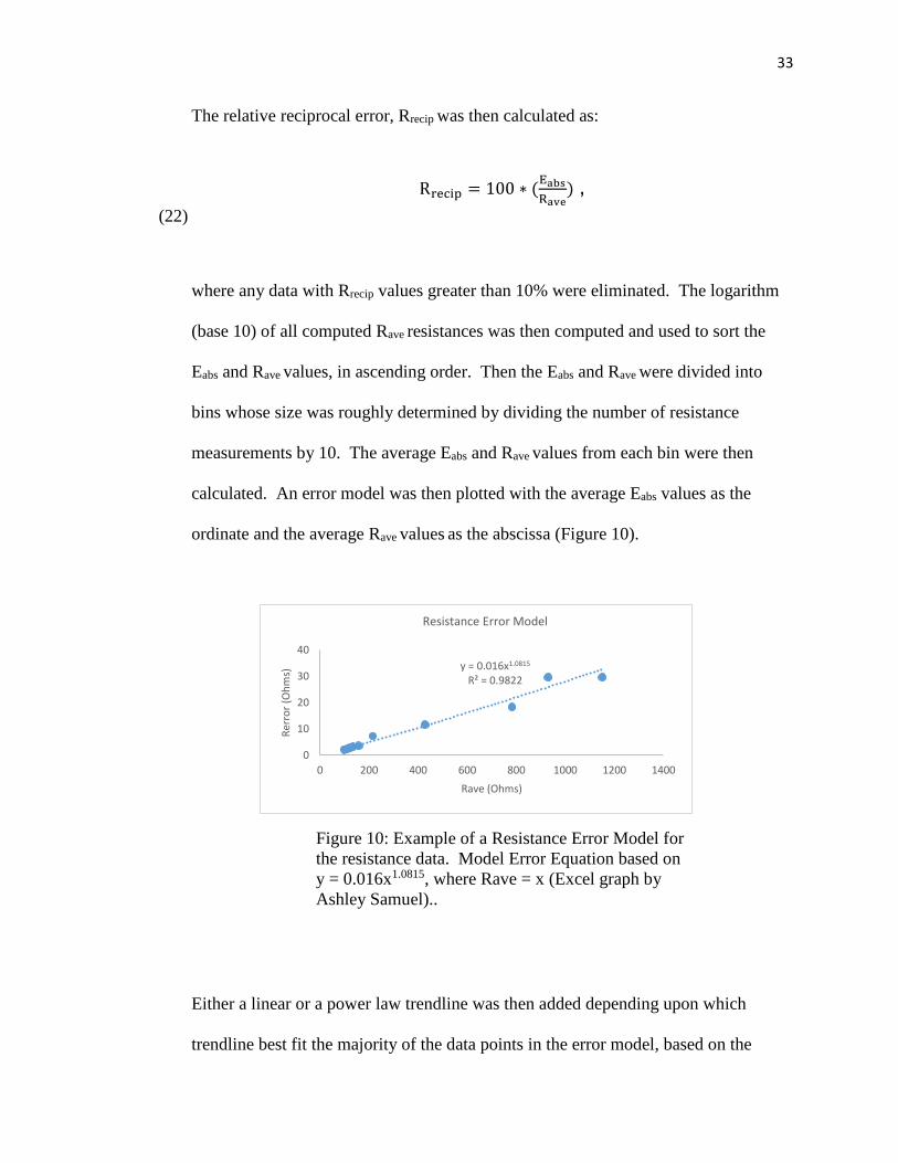
where any data with Rrecip values greater than 10% were eliminated. The logarithm

(base 10) of all computed Rave resistances was then computed and used to sort the

Eabs and Rave values, in ascending order. Then the Eabs and Rave were divided into

bins whose size was roughly determined by dividing the number of resistance

measurements by 10. The average Eabs and Rave values from each bin were then

calculated. An error model was then plotted with the average Eabs values as the

ordinate and the average Rave values as the abscissa (Figure 10).

Either a linear or a power law trendline was then added depending upon which

trendline best fit the majority of the data points in the error model, based on the

y = 0.016x1.0815

R² = 0.9822

0

10

20

30

40

0 200 400 600 800 1000 1200 1400

Rer

ror

(Oh

ms)

Rave (Ohms)

Resistance Error Model

Figure 10: Example of a Resistance Error Model for

the resistance data. Model Error Equation based on

y = 0.016x1.0815, where Rave = x (Excel graph by

Ashley Samuel)..

34

highest calculated R2 (linear regression) value using Microsoft Excel. If a linear

trendline was used, then a slope and y-intercept were obtained from the equation for

the trendline (Equation 23) and used to calculate the model errors. If a power law

trendline was used, a slope and exponent were obtained from the equation of the

trendline (Equation 24) and used to calculate the model errors. These trendline

equations and their corresponding slopes, y-intercepts and exponents were then

used to calculate the model errors according to either one of the following formulas:

εmodel = m ∗ Rave + b (23)

εmodel = m ∗ (Rave)a (24)

These model errors were eventually inputted into the R3t Inversion program,

however in certain cases where the solution did not converge in less than 5

iterations, an additional 2% error was added to all Rerror values according to the

following equation:

Rerror = Eabs + 0.02(Rave)

(25)

This additional 2% error allowed the solution to converge in less than 5 iterations

using the R3t inversion program (described in the following sections).

Phase Data Processing

35

After completing the error analysis for the resistance data as described previously,

the phase data were calculated by multiplying the chargeability, M by a factor of -

1.3 (Mwakanyamale, et. al, 2012). The phase error, error, was then calculated

(Equation 26) and an error analysis for the phase data was performed using a

similar method to that used for the resistance data error analysis.

error

= |𝑁 − 𝑅| (26)

The only difference between the two error analyses is that for the phase error

analysis, instead of plotting the error model in terms of the average Eabs values as

the ordinate and the average Rave values as the abscissa, the average error values

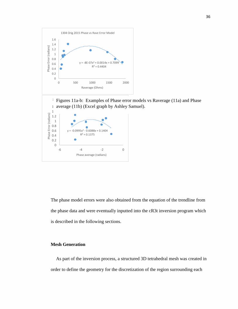
were plotted as the ordinate and the Rave values as the abscissa (Figures 11a-b).

36

The phase model errors were also obtained from the equation of the trendline from

the phase data and were eventually inputted into the cR3t inversion program which

is described in the following sections.

Mesh Generation

As part of the inversion process, a structured 3D tetrahedral mesh was created in

order to define the geometry for the discretization of the region surrounding each

y = -8E-07x2 + 0.0014x + 0.7099R² = 0.4404

0

0.2

0.4

0.6

0.8

1

1.2

1.4

1.6

0 500 1000 1500 2000

Ph

ase

Erro

r (r

adia

ns)

Raverage (Ohms)

1304 Orig 2015 Phase vs Rave Error Model

y = -0.0995x2 - 0.6088x + 0.1404R² = 0.1375

0

0.2

0.4

0.6

0.8

1

1.2

1.4

1.6

-6 -4 -2 0

Ph

ase

Erro

r (r

adia

ns)

Phase average (radians)

1304 Orig 2015 Phase vs Phase Error ModelFigures 11a-b: Examples of Phase error models vs Raverage (11a) and Phase

average (11b) (Excel graph by Ashley Samuel).

37

borehole array as well as the position of the borehole array with respect to

elevation. In mathematics, discretization concerns the process of transferring

continuous functions, models, and equations into discrete counterparts. The mesh

allows the R3t inversion program to calculate the resistivities at each node within

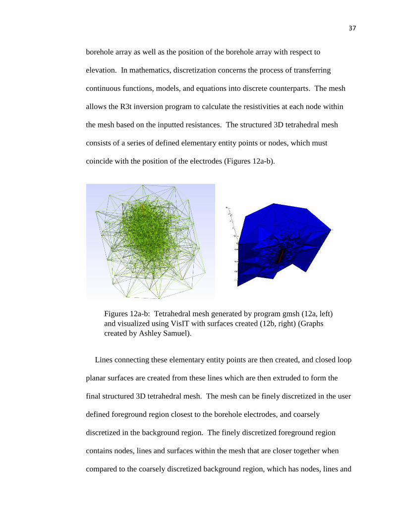
the mesh based on the inputted resistances. The structured 3D tetrahedral mesh

consists of a series of defined elementary entity points or nodes, which must

coincide with the position of the electrodes (Figures 12a-b).

Lines connecting these elementary entity points are then created, and closed loop

planar surfaces are created from these lines which are then extruded to form the

final structured 3D tetrahedral mesh. The mesh can be finely discretized in the user

defined foreground region closest to the borehole electrodes, and coarsely

discretized in the background region. The finely discretized foreground region

contains nodes, lines and surfaces within the mesh that are closer together when

compared to the coarsely discretized background region, which has nodes, lines and

Figures 12a-b: Tetrahedral mesh generated by program gmsh (12a, left)

and visualized using VisIT with surfaces created (12b, right) (Graphs

created by Ashley Samuel).

38

surfaces that are spread further apart. The foreground region of the mesh allows for

better resolution of the resulting inverted resistivity image. The mesh is broken up

into a foreground region closer to the borehole electrodes due to the fact that

resolution, or the ability of a resistivity measurement to resolve changes within the

subsurface, is also always better closer to the borehole electrodes. This is due to the

fact that resolution and current density diminish as the distance away from the

borehole electrodes increases, therefore only a coarsely discretized background

region is required the further away the mesh is from the borehole electrodes.

The structured 3D tetrahedral mesh was defined using the gmsh mesh generator

program (Christophe Geuzaine and Jean-Francois Remacle). The gmsh program

allows the user to define the mesh graphically or by entering in code into the

geometry file (.geo). The process for creating the mesh involves first defining the

borehole electrodes as elementary entity points or nodes, and including the

elevations of these electrodes within the borehole. Mesh boundaries with

elementary entity points (electrodes) are then defined, and the lines connecting each

entity are created, which in turn create closed loop planar surfaces. These 2D

geometrically closed loop planar surfaces are then extruded to create volumes

which form the structured 3D tetrahedral mesh. The term tetrahedral mesh applies

because all four node vertices of the resulting 3D discretized section are the same

distance from each other, and the planar surfaces have no parallel faces, the shapes

of which defines a tetrahedron. The 3D tetrahedral mesh is called “structured”

because all of the mesh elements align along a single vertical axis, and in this case

the axis refers to the vertical alignment of the borehole electrodes.

39

The final mesh file (.msh) was then converted into a mesh3d.dat file required by

the R3t inversion program by running it through a MatLab script. The MatLab

script reads the following data from the mesh file in order to convert it into the

proper mesh3d.dat file format required for the R3t inversion program: total number

of triangular prism elements, total number of nodes, triangular prism node numbers

and node coordinates. This mesh3d.dat file was used for both the field resistivity

and phase inversions that are described in the following sections.

Resistivity Inversion and Visualization

Inverse modeling is the science of finding a model to fit the observed data.

There are many methods for achieving this goal however the inversion software

used for the purpose of this research is R3t version 1.8, which was developed by

Andrew Binley of Lancaster University, England. R3t is an inverse solution

software program for 3D current flow in a tetrahedral mesh. The inverse solution is

based on a regularized objective function combined with weighted least squares (an

‘Occams’ type solution) as defined in Binley and Kemna (2005). The R3t program

uses an iterative process which solves the following equations repeatedly until

satisfactory convergence has been achieved:

( JTWdTWdJ + αR)∆m = JTWd

T(d − f(mi)) − αRm (27)

mi+1 = mi + ∆m (28)

where the parameters in Equations 27 and 28 are defined as: J is the Jacobian, such

that Ji,j = ∂di/ ∂mj, d is the data vector, mi is the parameter vector at iteration i, Wd

40

is the data weight matrix, assumed to be diagonal, with Wi,i = 1/∈i, where ∈𝑖 is the

standard deviation of measurement i, is the regularization (or smoothing)

parameter, R is the roughness matrix, which describes the connectivity of parameter

blocks, m is update in parameter values at each iteration and f(m) is the forward

model for parameters m. Satisfactory convergence is achieved once the data misfit

reaches a required tolerance. The data misfit is expressed as a root mean square

error:

RMS = √1

N∑(

di−fi(m)

∈i )2 (29)

where N is the number of measurements and the target data misfit (RMS) is equal

to 1.

The R3t inversion program requires three input files: R3.in, mesh3d.dat and

protocol.dat. In the R3.in file, parameters for the inversion are set based on the

desired type of inversion selected. For this inversion, background regularization

was used. Background regularization is when changes in resistivity are constrained

against a background model rather than a model in order reduce structure in the

image. The mesh3d.dat file requires the parameters for defining the 3D tetrahedral

mesh as described in the previous section. The protocol.dat file contains the

number of measurements as well as the electrode spacings, average resistances and

their associated model errors as calculated from the error models. After all of these

input files including the resistances were run through the program, R3t then

outputted the inverted resistivities into a file (f001.vtk). This file was then used to

41

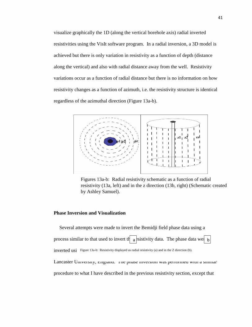
visualize graphically the 1D (along the vertical borehole axis) radial inverted

resistivities using the VisIt software program. In a radial inversion, a 3D model is

achieved but there is only variation in resistivity as a function of depth (distance

along the vertical) and also with radial distance away from the well. Resistivity

variations occur as a function of radial distance but there is no information on how

resistivity changes as a function of azimuth, i.e. the resistivity structure is identical

regardless of the azimuthal direction (Figure 13a-b).

Phase Inversion and Visualization

Several attempts were made to invert the Bemidji field phase data using a

process similar to that used to invert the resistivity data. The phase data were

inverted using the cR3t version 0.2a program developed by Andrew Binley of

Lancaster University, England. The phase inversion was performed with a similar

procedure to what I have described in the previous resistivity section, except that

Figure 13a-b: Resistivity displayed as radial resistivity (a) and in the Z direction (b).

a b

Figures 13a-b: Radial resistivity schematic as a function of radial

resistivity (13a, left) and in the z direction (13b, right) (Schematic created

by Ashley Samuel).

42

the resistivity is now considered as a complex variable defined in the data as a

magnitude and phase.

For this inversion, background regularization was used. The mesh3d.dat file

requires the parameters for defining the 3D tetrahedral mesh as described in the

previous section. The protocol.dat file contains the number of measurements as

well as the electrode spacings, average resistances and their associated model

errors, average phase values and their model errors as calculated from the error

models. These input files were run through the cR3t program, which outputted the

inverted resistivities and phase values into a file (f001.vtk). This file was then used

to visualize graphically the 1D (along the vertical borehole axis) radial inverted

resistivities and phase values (Appendix A) using the VisIt software program.

The phase inversion attempts were not successful for all data sets due to the fact

that the solutions did not converge in the required number of iterations. Therefore,

for almost all of the phase inversion attempts, a solution was not obtained. For the

phase inversions that did successfully converge, the results can be found in

Appendix A.

Ratio Resistivity Inversions

The Bemidji field data were analyzed using ratio inversions to measure

changes in resistivity over time at each of the two borehole arrays. Ratio inversions

require combined model errors calculated from each of the two borehole array data

sets collected during two different time periods. In order to calculate the combined

model error for the ratio inversion the following equation is required:

43

𝑑𝑒𝑟𝑟𝑜𝑟 = |𝑑| ∗ √(𝑎𝑒𝑟𝑟𝑜𝑟

𝑎)

2

+ (𝑏𝑒𝑟𝑟𝑜𝑟

𝑏)

2

+ (𝑐𝑒𝑟𝑟𝑜𝑟

𝑐)

2

(30)

where the variables in Equation 30 are as follows: a = Year 1 Resistance Data, aerror

= Model Error from Year 1 Resistance Data, b = Year 2 Resistance Data, berror =

Model Error from Year 2 Resistance Data, c = Forward Model Resistance Data for

a 100 Ohm Homogeneous Earth, cerror = Model Error from Forward Model

Resistance Data and d = (Year 2 Resistance Data)/(Year 1 Resistance Data).

The a = Year 1 Resistance Data or background data, can be taken from any of the

available data sets from any individual year. The same is true for the b = Year 2

Resistance Data, however it must be from a different year or time period from Year

1. The aerror and berror model errors are calculated from the individual error models

for each year’s data set. A forward model is used by the R3t inversion program to

create resistance data based on a synthetic model for a 100 Ohm-m homogeneous

earth. These forward model resistance and calculated transfer resistance data are

then used to compute the forward model errors. These transfer resistances and

forward modeling errors are calculated from the following formulas:

Rtransfer = a

4πa[

1

AM−

1

MB−

1

AN+

1

NB ] (31)

cerror = |Rtransfer − c| (32)

44

where the variables for Equations 31 and 32 are defined as follows: a = apparent

resistivity, Rtransfer = Transfer Resistance, c = Forward Model Resistance Data, 4a

= Geometric Factor for a Borehole Configuration, a = Electrode Spacing for the

Wenner Configuration (for these data there are both a=1 and a=2 measurements),

AM = Distance Between the Positive Current Electrode (C+) and the Positive

Potential Electrode (P+), MB = Distance Between the Positive Potential Electrode

(P+) and the Negative Current Electrode (C -), AN = Distance Between the Positive

Current Electrode (C+) and the Negative Potential Electrode (P -) and NB =

Distance Between the Negative Potential Electrode (P -) and the Negative Current

Electrode (C -).

After all of these calculations are performed, the resistance data that are inputted

into the R3t protocol.dat file are computed from the relationship:

Rratio = d ∗ c (33)

As previously defined, d is the ratio of the Year 2 Resistance Data divided by the

Year 1 Resistance Data, and c is the Forward Model Resistance Data calculated

from a synthetic 100 Ohm homogeneous earth. In addition to the protocol.dat file,

a R3.in file containing the parameters for the inversion are set based on the desired

type of inversion selected. In this case background regularization was used, and the

mesh3d.dat file containing the parameters were used to define the 3D tetrahedral

mesh as described in the previous sections.

45

Once these files were run through the R3t inversion program, the resulting

f001.vtk file containing the inverted ratio resistivity was used to visualize changes

in resistivity in the VisIt software program.

Laboratory Methods

A set of column laboratory experiments was set up in order to observe the SIP

response of uncontaminated Bemidji, MN cores mixed with magnetite and saturated

with two different pore fluid conductivities. The purpose of the laboratory

experiments was to determine the effects of mineralization and pore fluid

conductivity on geophysical SIP signatures. These data were then plotted using

MatLab in order to view the plotted phase, resistivity, real conductivity and

imaginary conductivity versus frequency.

SIP Measurements on Sample Filled Laboratory Columns

For the supporting laboratory research, a core was taken in 2014 by the USGS

personnel from the uncontaminated region just outside the free phase plume area in

Bemidji, MN. The core number was 1408-17, which was taken from the soil region

around the water table (approximate depth 1.7 – 2.5m from ground surface), and it

was approximately 24 inches in length when fully retrieved. Two soil samples were

taken from the top of the core while they were still encased in the original plastic

cylindrical core casing. The soil samples and their casings were placed in a vice

and cut using a Porter-Cable Saber saw. The resulting lengths and diameters of

each cut core were approximately 50mm and 45mm, respectively.

46

Although no thorough chemical analysis on the two samples could be obtained,

both samples were assumed to be identical geologically due to the fact that they

came from the same core and did not have any apparent visual differences. One

soil sample was designated as the relatively undisturbed control sample, and was

temporarily left inside its original plastic core casing so that laboratory magnetic

susceptibility measurements could be obtained (see following Magnetic

Susceptibility section for the procedure). The relatively undisturbed control sample

and casing were weighed prior to being packed into the first laboratory column.

The plastic casing was also weighed individually after the soil was extracted so that

an accurate mass of the soil sample by itself could be calculated by subtracting the

casing weight from the total sample with casing. The second soil sample was

weighed in a similar fashion while it was still in its casing and then extracted to be

mixed with 1% (by mass) abiotic magnetite with grain size <106 m. Once the

magnetite was mixed into the soil sample and a homogenous mixture was achieved,

the 1% magnetite soil sample was temporarily placed back into the original plastic

core casing so that magnetic susceptibility measurements could be obtained. These

two soil samples were then eventually transferred into two separate laboratory

columns for the purpose of comparing the effects with and without mineralization

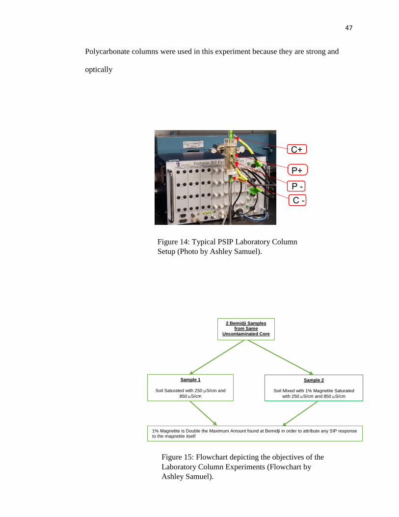
on geophysical SIP signatures (Figure 14). The flowchart describing the main

experimental procedure and goals for the two different laboratory columns can be

found in Figure 15.

The columns were made of Lexan, which is a brand name for a polycarbonate, or

a thermoplastic polymer containing carbonate groups in its chemical structure.

47

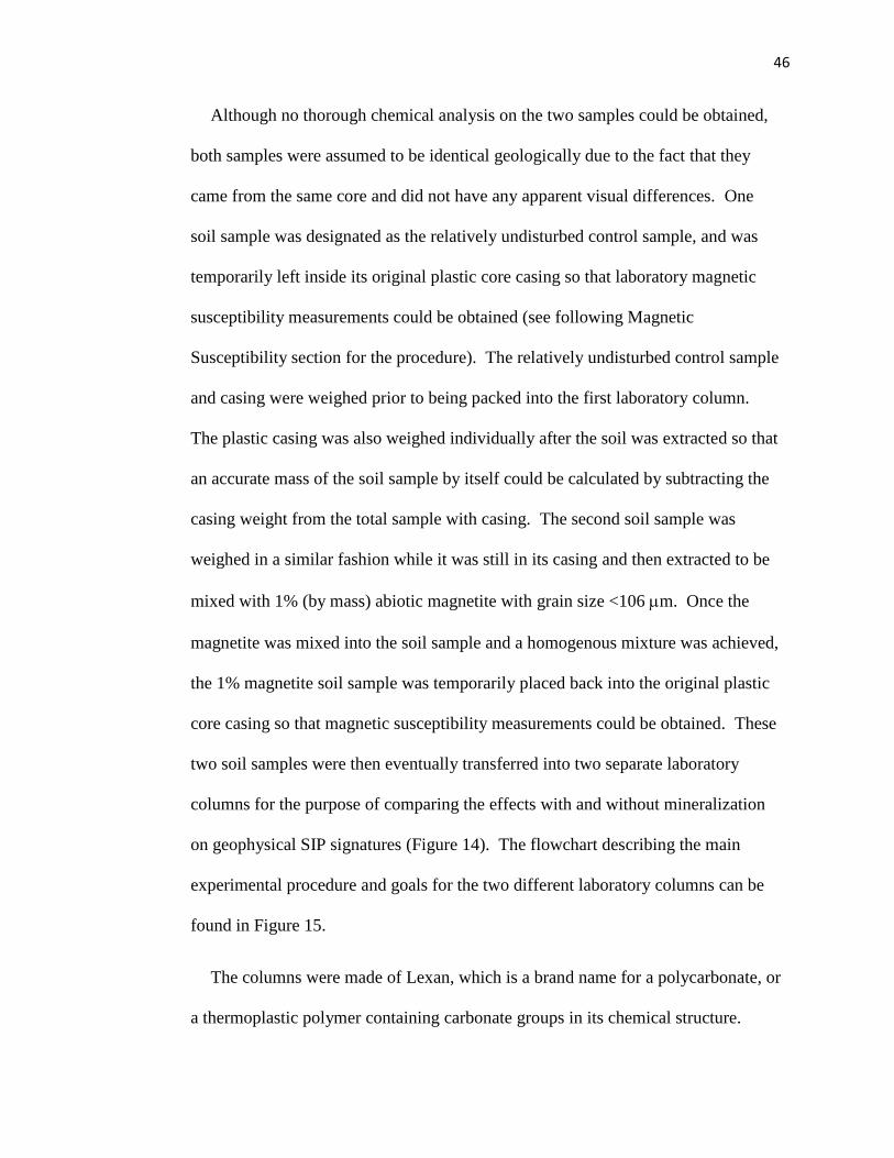
Polycarbonate columns were used in this experiment because they are strong and

optically

Figure 15: Flowchart depicting the objectives of the

Laboratory Column Experiments (Flowchart by

Ashley Samuel).

Sample 1

Soil Saturated with 250 S/cm and

850 S/cm

Sample 2

Soil Mixed with 1% Magnetite Saturated

with 250 S/cm and 850 S/cm

1% Magnetite is Double the Maximum Amount found at Bemidji in order to attribute any SIP response to the magnetite itself

2 Bemidji Samples from Same

Uncontaminated Core

C+

P+

P -

C -

Figure 14: Typical PSIP Laboratory Column

Setup (Photo by Ashley Samuel).

48

transparent. Each column consisted of a main hollow cylindrical body which had

two equally spaced holes on its exterior in order to allow for the placement of two

silver wire potential electrodes. Two circular, flat current electrodes made of

sintered silver and silver chloride (Ag-AgCl), were glued with an epoxy to the

inside of the column end caps which were then soldered to a small thin insulated

copper wire which protruded outside of the center of the column end caps to allow

for current injection. These column end caps were designed to be fitted perfectly to

the main cylindrical body of the column and prevent leakage. The column

dimensions were: inner column diameter = 23.52mm, outer column diameter =

29.89mm, total assembled column height = 92.88mm, AM (or the distance between

C+ and P+ electrodes) and NB (distance between P- and C- electrodes) = 48mm,

MN (distance between P+ and P- electrodes) = 25mm, MB (distance between P+

and C- electrodes) and AN (distance between C+ and P- electrodes) = 71mm and

AB (distance between C+ and C- electrodes protruding from column end caps) =

119mm.

In order to pack the samples, one of the bottom column end caps was first

attached to the bottom of the main cylindrical body, and a circular cloth mesh was

placed on top of the current electrode in order to protect it from the soil sample.

The soil sample was slowly and carefully packed into the base of the column until it

completely filled the entire column. Another cloth mesh was placed on top of the

second current electrode within the top column end cap and this end cap was fitted

49

to the top of the column in order to seal in the soil sample. Two silver wires were

coated to become silver and silver chloride (Ag-AgCl) potential electrodes, and

were encased in protective rubber fittings, necessary to prevent current from

flowing anywhere other than within the soil sample itself. The rubber encased

silver wire potential electrodes were then placed into plastic screw fittings. These

plastic screw fittings were then screwed into the preexisting threaded holes outside

of the main cylindrical body of the column in order to prevent leakage around the

potential electrodes.

Tygon Poly Vinyl Chloride (PVC) tubing (3.5mm inner diameter), selected for

its resistance to flex-fatigue and abrasion, was then attached to plastic screw fittings

which screwed into a preexisting threaded hole that went through each column end

cap. Each tube was attached to a manual shut off valve in order to control inflow

and outflow through the column. The tube connected to the base of the column was

placed in a pyrex flask filled with artificial groundwater, and held in place using

parafilm and electrical tape. The tube was also attached to a peristaltic pump which

drew the artificial groundwater from the flask into the column, with inflow from the

bottom of the column and outflow from the top of the column. This allowed each

sample within the column to become saturated. Saturation was achieved by

allowing 5 pore volumes of artificial groundwater to flow through each column.

The volume of fluid equivalent to 1 pore volume was calculated using the following

equation:

PV % = φ(πr2h) ,

(34)

50

where is the estimated porosity, r is the radius of the soil sample packed into the

column and h is the height of the soil sample packed in the column. For both

column setups, the estimated porosity was 0.4, the radius of the soil sample was

23.48 mm and the height of the soil sample was 92.48 mm. Equation 34 was

multiplied by 5 in order to calculate the equivalent volume of fluid needed to equal

5 pore volumes, which was equivalent to ~80 mL. The top column tube was placed

into a graduated pyrex flask so that the total volume of fluid outflow equivalent to

80mL could be measured to ensure full sample saturation.

Once full saturation was achieved, the contact resistances between all current

and potential electrodes were checked using a multi-meter and found to be less than

100 K-Ohms. Obtaining lower contact resistances is a way to verify that current

will be allowed to flow through the entire sample before any SIP measurements are

taken. Both the control sample and the 1% magnetite sample were fully saturated

inside the column using lab created artificial groundwater.

The artificial groundwater was created by adding the following masses of

chemicals to 1 L of deionized (DI) water in a large flask: 1.07mg Ammonium

Chloride (NH4Cl), 74.55mg Potassium Chloride (KCl), 98.59mg Magnesium

Sulfate (MgSO4), 58.81mg Calcium Chloride (CaCl2), 112.06mg Sodium Lactate

(C3H5NaO3) and 3,353.7mg or 3.35g Pipes Buffer (C8H16.5N2O6S2.1.5Na). After

the addition of these chemicals, a magnetic stirring rod was placed inside the fluid

filled flask and set on top of a magnetic stirrer plate for approximately 1 hour in

order to thoroughly mix the chemicals with the DI water. Two different types of

51

artificial groundwater were created, with two different fluid conductivities

equivalent to the Bemidji, MN naturally occurring minimum (0.025 S/m) and

maximum (0.085 S/m) field pore fluid conductivities. These two different fluid

conductivities were created in order to saturate the columns and observe the effects

of using two different pore fluid conductivities on laboratory geophysical

signatures. The first artificial groundwater solution originally had a fluid

conductivity of 0.149 S/m which was diluted with DI water until a fluid

conductivity of 0.085 S/m was measured by the conductivity probe. A portion of

the 0.085 S/m artificial groundwater solution was then diluted with DI water in

order to reduce the fluid conductivity to 0.025 S/m. SIP measurements were taken

immediately after each column was fully saturated with the lower fluid conductivity

(0.025 S/m) artificial groundwater solution and had low contact resistances. After

these SIP measurements were taken on both columns, they were then re-saturated

with the higher fluid conductivity (0.085 S/m) artificial groundwater solution and

checked for low contact resistances before additional SIP measurements were

obtained. Additionally, the fluid conductivities of the column outflow were

recorded (control column = 0.026 S/m and 0.086 S/m respectively, magnetite

column = 0.027 S/m and 0.088 S/m respectively) and were found to be similar to

the inflow conductivities. This slight increase in resulting outflow versus original

inflow conductivity indicated that there was only minor mineral dissolution

occurring due to the saturation procedure.

SIP measurements were obtained by first attaching wires with alligator clips to

the current and potential electrodes of each column. These wires were plugged into

52

the Portable Spectral Induced Polarization (SIP) Field/Laboratory Unit (PSIP),

which is a multi-channel geophysical instrument designed by Ontash and Ermac.

The PSIP has a 10V output voltage, 10 mA stimulating current and measures phases

less than 1 mRadians over a 1 mHz to 1 KHz frequency spectrum. The PSIP

recorded a series of phase and resistance measurements over a 0.01 Hz to 10 KHz

frequency spectrum on both laboratory columns from December 2015 to January

2016. The final laboratory column setup for obtaining SIP measurements can be

observed in Figure 14.

Laboratory SIP Data Processing

The PSIP instrument recorded the frequency, phase and relative resistance of

each laboratory column for every measurement. A MatLab script was written in

order to process these data to obtain the resistivity, real and imaginary conductivity

and can be found in Appendix B. First the geometric factor was calculated for each

column using the following formula:

K =πr2h

MN , (35)

where K is the geometric factor for the laboratory column, r is the inner radius of

the column, h is the height of the column and MN is the distance between the

potential electrodes. The geometric factor was found to be equal to 0.0173 mm2,

and was then used to calculate the resistivity, real and imaginary conductivity based

on the following relationships:

53

R = 100*(Rrel ) (36)

ρa = K ∗ R (37)

= (−1) ∗ rec

(38)

Where R is the resistance calculated from multiplying the Relative Resistance, Rrel,

by 100, a is the apparent resistivity and is the calculated phase for the purpose of

plotting it on a positive ordinate (y-axis) obtained by multiplying the recorded

negative phase, rec, by a -1 from the PSIP instrument. The real conductivity and

imaginary conductivity were calculated in the MatLab script using Equations 7 and

8, respectively, where in this case the is actually the apparent resistivity, a.

Laboratory Magnetic Susceptibility Measurements

Laboratory magnetic susceptibility measurements were obtained on the two

sample cores prior to their being packed into the columns. Each core was still in

its’ original plastic cylindrical casing from the field. As described previously, the

control core was kept relatively undisturbed in its original casing, whereas the other

core was emptied into a container and mixed with 1% magnetite before being

placed back into its original casing. To keep the soil from falling out of the casing,

Parafilm and electrical tape were wrapped around the two open ends of each core

sample. A Bartington MS2C magnetic susceptibility meter with a circular core

sample holder for mounting the core samples vertically, was used to obtain the

measurements. An example of this type of MS2C magnetic susceptibility meter

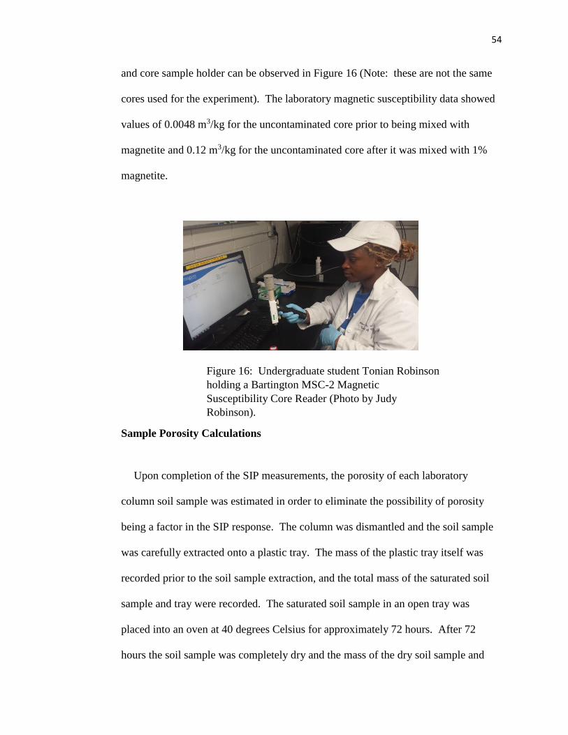
54

and core sample holder can be observed in Figure 16 (Note: these are not the same

cores used for the experiment). The laboratory magnetic susceptibility data showed

values of 0.0048 m3/kg for the uncontaminated core prior to being mixed with

magnetite and 0.12 m3/kg for the uncontaminated core after it was mixed with 1%

magnetite.

Sample Porosity Calculations

Upon completion of the SIP measurements, the porosity of each laboratory

column soil sample was estimated in order to eliminate the possibility of porosity

being a factor in the SIP response. The column was dismantled and the soil sample

was carefully extracted onto a plastic tray. The mass of the plastic tray itself was

recorded prior to the soil sample extraction, and the total mass of the saturated soil

sample and tray were recorded. The saturated soil sample in an open tray was

placed into an oven at 40 degrees Celsius for approximately 72 hours. After 72

hours the soil sample was completely dry and the mass of the dry soil sample and

Figure 16: Undergraduate student Tonian Robinson

holding a Bartington MSC-2 Magnetic

Susceptibility Core Reader (Photo by Judy

Robinson).

55

tray were recorded. The mass of the plastic tray by itself was subtracted from the

recorded masses of the saturated sample and tray along with the dry sample and

tray. This calculation was necessary in order to obtain the individual masses of the

saturated sample and dry sample. The porosity of each soil sample was then

estimated according to the following equation:

φest =Vv

VT=

(msat−mdry)

(𝜌𝑤𝑎𝑡𝑒𝑟)(Vcolumn) ,

(39)

where 𝜑𝑒𝑠𝑡 is the estimated porosity, Vv is the volume of voids which in this case is

equal to the volume of water lost during drying, VT is the total volume of the

original soil sample in the column, msat is the mass of the saturated soil sample by

itself, mdry is the mass of the dry soil sample by itself, 𝜌𝑤𝑎𝑡𝑒𝑟 is the density of water

(1g/cm3) and Vcolumn is the total interior volume of the laboratory column that held

the soil sample. The porosity of the control sample was found to be 0.294 and the

magnetite sample’s porosity was 0.297, with a percent difference between the two

measurements being equal to 1.1%.

5. RESULTS

Geological Grain Size Analysis

Geologically, USGS drillers found that the oil spill site at Bemidji, MN consists

of pitted sand and gravel outwash and moderately calcareous silty sand

(approximately 20 m thick) and outwash glacial deposits overlying clayey till of

unknown thickness (Bennett et al., 1993). A grain size analysis performed by

56

Mewafy, et. al, 2013 concluded that at the uncontaminated location (C1006) the

average percentages of gravel, sand, silt and clay were: 4.8%, 93.12% and 2.08%

respectively. At the contaminated location (C1010) the average percentages of

gravel, sand, silt and clay were: 1.13%, 96.94% and 1.93% respectively (Mewafy,

et. al, 2013).

A statistical analysis using a Welch's t-test (Equation 40) was performed to

compare the soils between the uncontaminated and contaminated regions. The

Welch’s t-test is used only when the two population variances are not assumed to be

equal (the two sample sizes may or may not be equal) and hence must be estimated

separately (The t-statistic to test whether the population means are different was

calculated as:

tvalue =μ1− μ2

√σ1

2

n1 +

σ22

n2

, (40)

where tvalue represents the Welch’s t-test parameter which determines the statistical

differences between the two different population means, 1 and 2 are the

corresponding mean percentages of each soil texture for all sample depths from the

uncontaminated and contaminated regions, 1 and 2 are the standard deviations of

each soil texture for all sample depths from the uncontaminated and contaminated

regions and n1 and n2 are the sample sizes from the uncontaminated and

contaminated regions. The Welch’s t-test found that since the calculated t-values

were all less than the critical t-scores, the two soils from the uncontaminated and

contaminated locations were not statistically different, within a 95-99% confidence

level (Figure 17).

57

Raw Apparent Conductivity and Specific Conductance Data

A preliminary analysis of the raw apparent conductivity data at the research site

in Bemidji showed a higher apparent conductivity in the contaminated region

compared with the uncontaminated region (Figure 18). This correlated well with

higher specific conductances of the pore fluid in the contaminated region versus the

uncontaminated region. These preliminary findings justified the need for the use of

inverse modelling in this study to improve the data analysis results.

Uncontaminated Contaminated T-Test Values

Gravel

%

Sand

%

Silt

&

Clay

%

Gravel

%

Sand

%

Silt

&

Clay

%

Gravel

%

1.56

4.80 93.12 2.08 1.13 96.94 1.93 Sand

%

-1.33

Silt &

Clay

%

0.11

Table 1: The Welch’s t-test found that since the calculated t-values were all

less than the critical t-scores, the two soils from the uncontaminated and

contaminated locations were not statistically different, within a 95-99%

confidence level (Table created by Ashley Samuel).

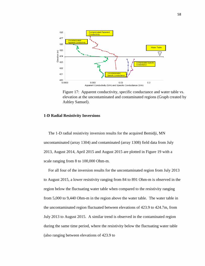
58

1-D Radial Resistivity Inversions

The 1-D radial resistivity inversion results for the acquired Bemidji, MN

uncontaminated (array 1304) and contaminated (array 1308) field data from July

2013, August 2014, April 2015 and August 2015 are plotted in Figure 19 with a

scale ranging from 8 to 100,000 Ohm-m.

For all four of the inversion results for the uncontaminated region from July 2013

to August 2015, a lower resistivity ranging from 84 to 891 Ohm-m is observed in the

region below the fluctuating water table when compared to the resistivity ranging

from 5,000 to 9,440 Ohm-m in the region above the water table. The water table in

the uncontaminated region fluctuated between elevations of 423.9 to 424.7m, from

July 2013 to August 2015. A similar trend is observed in the contaminated region

during the same time period, where the resistivity below the fluctuating water table

(also ranging between elevations of 423.9 to

Figure 17: Apparent conductivity, specific conductance and water table vs.

elevation at the uncontaminated and contaminated regions (Graph created by

Ashley Samuel).

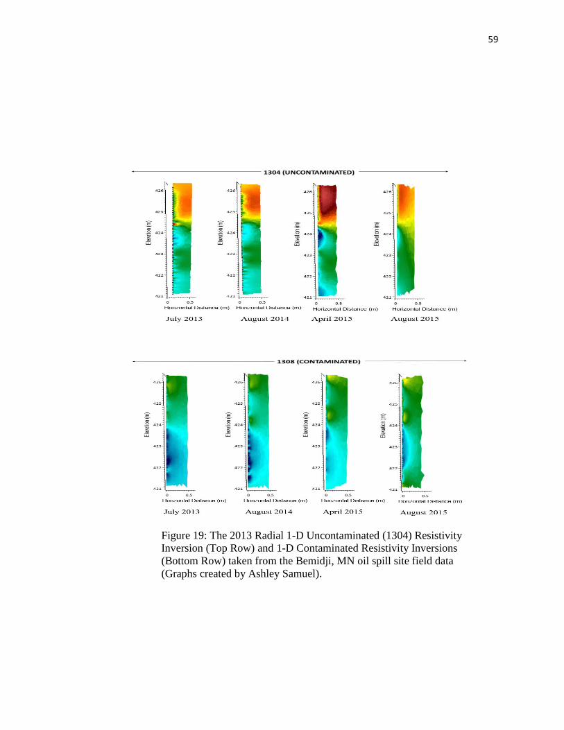
59

Figure 19: The 2013 Radial 1-D Uncontaminated (1304) Resistivity

Inversion (Top Row) and 1-D Contaminated Resistivity Inversions

(Bottom Row) taken from the Bemidji, MN oil spill site field data

(Graphs created by Ashley Samuel).

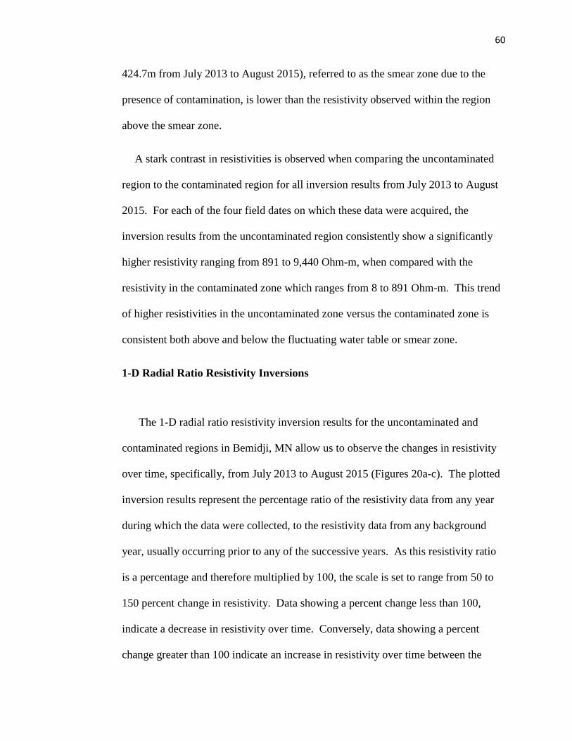
60

424.7m from July 2013 to August 2015), referred to as the smear zone due to the

presence of contamination, is lower than the resistivity observed within the region

above the smear zone.

A stark contrast in resistivities is observed when comparing the uncontaminated

region to the contaminated region for all inversion results from July 2013 to August

2015. For each of the four field dates on which these data were acquired, the

inversion results from the uncontaminated region consistently show a significantly

higher resistivity ranging from 891 to 9,440 Ohm-m, when compared with the

resistivity in the contaminated zone which ranges from 8 to 891 Ohm-m. This trend

of higher resistivities in the uncontaminated zone versus the contaminated zone is

consistent both above and below the fluctuating water table or smear zone.

1-D Radial Ratio Resistivity Inversions

The 1-D radial ratio resistivity inversion results for the uncontaminated and

contaminated regions in Bemidji, MN allow us to observe the changes in resistivity

over time, specifically, from July 2013 to August 2015 (Figures 20a-c). The plotted

inversion results represent the percentage ratio of the resistivity data from any year

during which the data were collected, to the resistivity data from any background

year, usually occurring prior to any of the successive years. As this resistivity ratio

is a percentage and therefore multiplied by 100, the scale is set to range from 50 to

150 percent change in resistivity. Data showing a percent change less than 100,

indicate a decrease in resistivity over time. Conversely, data showing a percent

change greater than 100 indicate an increase in resistivity over time between the

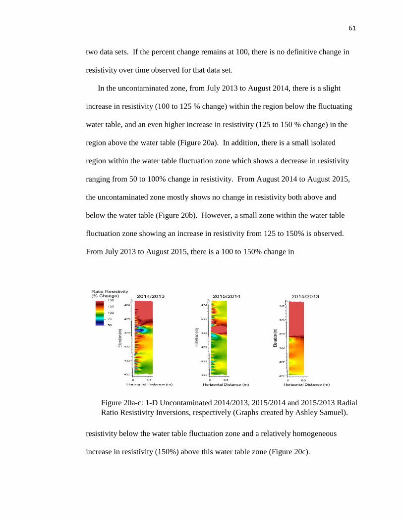
61

two data sets. If the percent change remains at 100, there is no definitive change in

resistivity over time observed for that data set.

In the uncontaminated zone, from July 2013 to August 2014, there is a slight

increase in resistivity (100 to 125 % change) within the region below the fluctuating

water table, and an even higher increase in resistivity (125 to 150 % change) in the

region above the water table (Figure 20a). In addition, there is a small isolated

region within the water table fluctuation zone which shows a decrease in resistivity

ranging from 50 to 100% change in resistivity. From August 2014 to August 2015,

the uncontaminated zone mostly shows no change in resistivity both above and

below the water table (Figure 20b). However, a small zone within the water table

fluctuation zone showing an increase in resistivity from 125 to 150% is observed.

From July 2013 to August 2015, there is a 100 to 150% change in

resistivity below the water table fluctuation zone and a relatively homogeneous

increase in resistivity (150%) above this water table zone (Figure 20c).

Figure 20a-c: 1-D Uncontaminated 2014/2013, 2015/2014 and 2015/2013 Radial

Ratio Resistivity Inversions, respectively (Graphs created by Ashley Samuel).

62

The contaminated 1-D ratio resistivity inversions (Figures 21a-c) show both a

decrease and/or increase from July 2013 to August 2014, there is a slight increase

and/or decrease in resistivity (100 to 125 % change) within the region below the

fluctuating water table, and an even higher increase in resistivity (125 to 150 %

change) in the region above the water table (Figure 19a). In addition, there is a

small isolated region within the water table fluctuation zone which shows an

increase and/or decrease in resistivity ranging from 50 to 100% change in

resistivity. From August 2014 to August 2015, the contaminated zone mostly

shows no change in resistivity both above and below the water table (Figure 21b).

However, a small zone within the water table fluctuation zone showing an increase

in resistivity from 125 to 150% change in resistivity is observed. From July 2013 to

August 2015, there is a 100 to 150% change in resistivity below the water table

fluctuation zone and a relatively homogeneous increase in resistivity (150%) above

this water table zone (Figure 21c).

Figure 21a-c: 1-D Contaminated 2014/2013, 2015/2014 and 2015/2013 Ratio

Resistivity Inversions, respectively (Graphs created by Ashley Samuel).

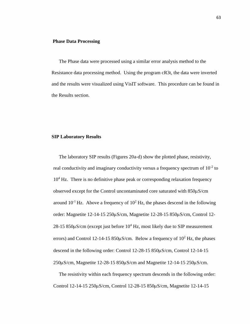
63

Phase Data Processing

The Phase data were processed using a similar error analysis method to the

Resistance data processing method. Using the program cR3t, the data were inverted

and the results were visualized using VisIT software. This procedure can be found in

the Results section.

SIP Laboratory Results

The laboratory SIP results (Figures 20a-d) show the plotted phase, resistivity,

real conductivity and imaginary conductivity versus a frequency spectrum of 10-2 to

104 Hz. There is no definitive phase peak or corresponding relaxation frequency

observed except for the Control uncontaminated core saturated with 850S/cm

around 10-1 Hz. Above a frequency of 102 Hz, the phases descend in the following

order: Magnetite 12-14-15 250S/cm, Magnetite 12-28-15 850S/cm, Control 12-

28-15 850S/cm (except just before 104 Hz, most likely due to SIP measurement

errors) and Control 12-14-15 850S/cm. Below a frequency of 102 Hz, the phases

descend in the following order: Control 12-28-15 850S/cm, Control 12-14-15

250S/cm, Magnetite 12-28-15 850S/cm and Magnetite 12-14-15 250S/cm.

The resistivity within each frequency spectrum descends in the following order:

Control 12-14-15 250S/cm, Control 12-28-15 850S/cm, Magnetite 12-14-15

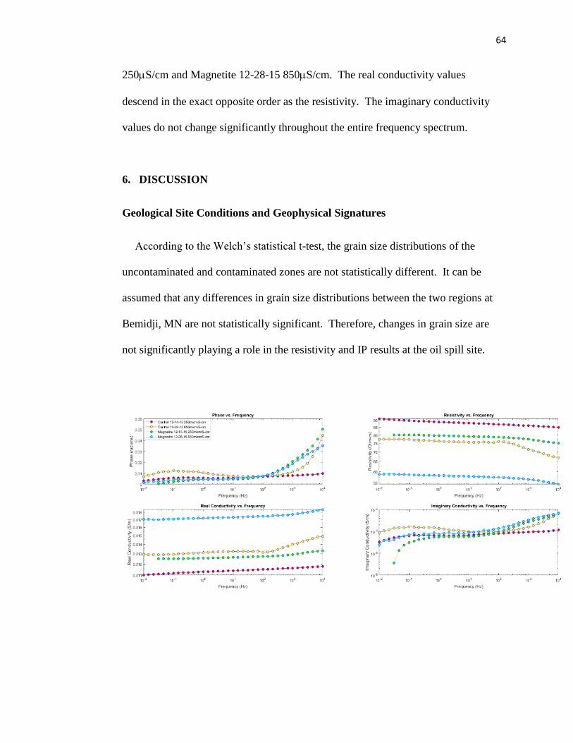
64

250S/cm and Magnetite 12-28-15 850S/cm. The real conductivity values

descend in the exact opposite order as the resistivity. The imaginary conductivity

values do not change significantly throughout the entire frequency spectrum.

6. DISCUSSION

Geological Site Conditions and Geophysical Signatures

According to the Welch’s statistical t-test, the grain size distributions of the

uncontaminated and contaminated zones are not statistically different. It can be

assumed that any differences in grain size distributions between the two regions at

Bemidji, MN are not statistically significant. Therefore, changes in grain size are

not significantly playing a role in the resistivity and IP results at the oil spill site.

65

Magnetic Susceptibility and Geophysical Signatures

The magnetic susceptibility at the Bemidji, MN oil spill site peaks around the

fluctuating water table zone at about 13.5 m3/kg within the fluctuating water table

zone (Figure 21a-b). However, in the contaminated zone, a magnetic susceptibility

peak is observed around 15.6 m3/kg within the smear zone. This indicates a higher

degree of magnetic iron minerals in the contaminated zone due to biodegradation

when compared to the uncontaminated zone.

The laboratory cores had a magnetic susceptibility of 0.0048 m3/kg for the

uncontaminated core prior to being mixed with magnetite and 0.12 m3/kg for the

uncontaminated core once it was mixed with 1% magnetite. For both the field and

laboratory data, the contaminated zones had magnetic susceptibility values 16-24%

higher than the uncontaminated zones. This corresponds well with the field

magnetic susceptibility values being higher for the smear zone within the

contaminated region than the uncontaminated region, due to the fact that it contains

more iron minerals such as magnetite.

Hydrology and Geophysical Signatures

The 1-D radial resistivity inversion results for the acquired Bemidji, MN

uncontaminated (array 1304) and contaminated (array 1308) field data from July

Figures 22a-d: SIP Laboratory results showing Phase vs. Frequency (22a, Top Left

Corner), Resistivity vs. Frequency (22b, Top Right Corner), Real Conductivity vs.

Frequency (22c, Bottom Left Corner) and Imaginary Conductivity vs. Frequency (22d,

Bottom Right Corner) (Graphs created by Ashley Samuel).

66

2013, August 2014, April 2015 and August 2015, show changes in their

geophysical signatures most likely due to changes in hydrology.

For all four of the 1-D Radial Resistivity inversion results for the

uncontaminated and contaminated regions from July 2013 to August 2015, a lower

resistivity is observed in the region below the fluctuating water table when

compared to the resistivity ranging in the region above the water table, due to

saturation below the water table. The main difference is that in the contaminated

zone, where there is still crude oil present, the fluctuating water table zone or the

smear zone has a lower resistivity when compared to the uncontaminated zone.

This geophysical effect is most likely due to the fact that the biodegraded crude oil

is mixed with the saturated smear zone or fluctuating contaminated water table.

Groundwater temperature variations in Bemidji, MN on the dates which the

resistivity data were collected were recorded for July 2013, August 2014, April

2015 and August 2015. The mean temperatures in Bemidji, MN increased and then

decreased from July 2013 to August 2014, and from August 2014 to April 2015,

and then increased from April 2015 to August 2015. Variations in the groundwater

temperature don’t explain the resistivity variations that are observed in these data.

The hydrology data and temperature data are consistent with these findings,

however they are not all completely relevant to the individual yearly resistivity

measurements. To procure the relevance of these data, the 1-D radial ratio

resistivity inversion results must be analyzed in order to examine the effects of time

on their geophysical signatures.

67

The 1-D radial ratio resistivity inversion results for the uncontaminated and

contaminated regions in Bemidji, MN allow us to observe the changes in resistivity

from July 2013 to August 2015. In the uncontaminated zone, from July 2013 to

August 2014, there is a slight increase in resistivity within the region below the

fluctuating water table, and an even higher increase in resistivity in the region

above the water table. This is despite the fact that the water levels actually increase

from July 2013 to August 2014. One would expect the water levels to decrease if

the resistivity is increasing, however, most likely this is due to water quality and not

quantity. As water quality data were not obtained, this is merely conjecture. Oil

levels dropped from July 2013 to August 2014, having an almost negligible effect

on geophysical signatures because they represent an extremely thin layer of oil on

top of the smear zone. In addition, there is a small isolated region within the

uncontaminated water table fluctuation zone which shows a decrease in resistivity,

which is probably due to near electrode effects.

From August 2014 to August 2015, the uncontaminated zone mostly shows no

change in resistivity both above and below the water table. However, a small zone

within the water table fluctuation zone showing an increase in resistivity is

observed, and is again most likely due to hydrology. From July 2013 to August

2015, there is a change in resistivity below the water table fluctuation zone and a

relatively homogeneous increase in resistivity above this water table zone which

could be due to the decrease in water levels and precipitation data from those two

time periods.

68

The contaminated 1-D ratio resistivity inversions show both a decrease and/or

increase from July 2013 to August 2014. There is either no change or a slight

increase in resistivity within the region below the fluctuating water table, and an

even higher increase in resistivity in the region above the water table. While it is

difficult to tell whether these changes in resistivity are due to near electrode effects

or are due to changes in hydrology, oil levels and/or groundwater temperature, most

likely they are due to hydrology. In addition, there is a small isolated region within

the water table fluctuation zone which shows an increase and/or decrease in

resistivity. From August 2014 to August 2015, the uncontaminated zone mostly

shows no change in resistivity both above and below the water table. However, a

small zone within the water table fluctuation zone showing an increase in resistivity

is observed. From July 2013 to August 2015, changes in resistivity below the water

table fluctuation zone and a relatively homogeneous increase in resistivity above

this water table zone are observed. These general increases in resistivity are most

likely due to the changes in hydrology.

Magnetic Susceptibility Field and Laboratory Results

The field Magnetic Susceptibility data results from Atekwana (2014) show a

definitive peak around the smear zone within the contaminated zone and a smaller

peak around the uncontaminated water table fluctuation zone. The peak within the

contaminated zone most likely corresponds to the higher iron mineral content (or

increased ferrimagnetism) and is possibly due to the biomineralization of magnetite.

This would also partially explain the increased conductivity of the smear zone

region also found in the 1-D Radial Resistivity Inversions. This is due to the fact

69

that the higher the ferrimagnetism, the higher the conductivity of the iron mineral

itself, in this case, magnetite. The smaller peak within the uncontaminated zone is

possibly due to a smaller degree of mineralization occurring which is probably not

due to biodegradation of any crude oil.

For both the field uncontaminated and contaminated zones, the magnetic

susceptibilities were mostly 13.0 m3/kg throughout the measured subsurface with

the exception of the peaks within the fluctuating water table zone or smear zone. In

the uncontaminated zone, a magnetic susceptibility peak of around 13.5 m3/kg is

observed within the fluctuating water table zone. However, in the contaminated

zone, a magnetic susceptibility peak is observed around 15.6 m3/kg within the

smear zone (Atekwana, 2014).

The laboratory magnetic susceptibility results are consistent with the field data in

that for the uncontaminated cores without magnetite, they are showing a much

lower value than for the uncontaminated cores with magnetite. This is again due to

the fact that the higher magnetite containing core has a higher magnetic

susceptibility due to the magnetite’s higher ferrimagnetism.

Laboratory SIP Results

The laboratory SIP results show the plotted phase, resistivity, real conductivity

and imaginary conductivity versus a frequency spectrum of 10-2 to 104 Hz. There is

no definitive phase peak or corresponding relaxation frequency observed except for

the control uncontaminated core saturated with 850S/cm around 10-1 Hz. Above a

frequency of 102 Hz, the phases descend in the following order in terms of their file

70

names: Magnetite 12-14-15 250S/cm, Magnetite 12-28-15 850S/cm, Control 12-

28-15 850S/cm (except just before 104 Hz, most likely due to SIP measurement

errors) and Control 12-14-15 850S/cm. Below a frequency of 102 Hz, the phases

descend in the following order in terms of their file names: Control 12-28-15

850S/cm, Control 12-14-15 250S/cm, Magnetite 12-28-15 850S/cm and

Magnetite 12-14-15 250S/cm. There is no indication that either the magnetite or

the pore fluid conductivity seem to be controlling the decreasing phase values for

any frequency range.

The resistivity within each frequency spectrum descends in the following order:

Control 12-14-15 250S/cm, Control 12-28-15 850S/cm, Magnetite 12-14-15

250S/cm and Magnetite 12-28-15 850S/cm. The real conductivity values

descend in the exact opposite order as the resistivity. Both the pore fluid

conductivity and iron mineral (magnetite) content seem to be controlling the

resistivity and real conductivity values. The higher the pore fluid conductivity and

the magnetite content, the lower the resistivity values and higher the real

conductivity values.

The imaginary conductivity values do not change significantly throughout the

entire frequency spectrum. Perhaps this indicates that magnetite does not affect the

imaginary conductivity response.

Solid Phase Changes and Geophysical Signatures

Solid phase changes are not responsible for changes in geophysical signatures at

Bemidji, Minnesota. Solid phase changes include mineralization/biomineralization

71

of iron minerals such as magnetite. In the field data, biomineralization of magnetite

is not effecting the resistivity changes that are occurring within the smear zone and

the uncontaminated fluctuating water table zone. The laboratory data suggest that

mineralization (albeit in this case abiotic) does not have a substantial effect on

geophysical signatures such as resistivity and real conductivity. The generation of

solid precipitates such as magnetite by biodegradation does not produce substantial

laboratory electrical spectral induced polarization (SIP) and magnetic susceptibility

responses.

Aqueous Phase Changes and Geophysical Signatures

Aqueous phase changes are also contributing to changes in geophysical

signatures at Bemidji, Minnesota. Aqueous phase changes include pore fluid

conductivity changes. Pore fluid conductivity may exert an even greater

contributory significance to geophysical signatures than does solid phase changes

such as mineralization/biomineralization. Electrolytic conductivity is the electrical

conductivity of the pore fluid within the subsurface. At the site in Bemidji, the

metabolic byproducts produced by biodegradation such as organic acids are

elevating the electrolytic conductivity within the contaminant plume. When the

conductivity increases, the resistivity decreases, due to their inverse relationship

with one another.

Future Research Considerations

If any additional research were to be performed, there would be numerous

possibilities for future research considerations. Perhaps additional laboratory

72

experiments using the PSIP instrument setup for both SIP and TDIP measurements

could be obtained. The Fourier transform could be utilized to convert the field

TDIP data to SIP data for comparison purposes. Finally, it would help

tremendously to know the exact geochemistry of the field cores using a

synchrotron.

7. CONCLUSIONS

Site grain size distribution was ruled out as being a factor in changes in

geophysical signatures. The addition of magnetite was not responsible for changes

in resistivity in the laboratory results. The magnetic susceptibility field and

laboratory data agree in that they both show a higher degree of ferrimagnetism

within the contaminated zone or where mineralization is present. However, this still

does not explain the higher conductivity, or lower resistivity found in these regions

for the 1-D Radial Resistivity Inversions. Hydrology definitely plays a role in the

1-D Radial Resistivity Inversion results. The more saturated or more conductive the

water is which saturates the uncontaminated water table fluctuation zone or smear

zone, the lower the resistivity in those regions. Oil levels, consisting of an extremely

thin layer on top of the water table, most likely do not play a significant role in

changes in resistivity throughout the uncontaminated and contaminated regions.

Groundwater temperature variations most likely do not effect resistivity changes in

the field.

The laboratory SIP results lead us to conclude that aqueous phase changes are

responsible for changes in SIP response and therefore geophysical signatures and not

73

solid phase changes. The SIP data clearly show that phase is not affected by

changes in pore fluid conductivity or the addition of magnetite. However, resistivity

and real conductivity are definitely affected more so by pore fluid conductivity and

not by mineralization or the addition of magnetite. Imaginary conductivity is not

affected whatsoever by the pore fluid conductivity or the addition of magnetite.

The pore fluid conductivity is an example of aqueous phase changes which

eventually affects geophysical signatures and the addition of magnetite is an

example of solid phase changes which does not affect geophysical signatures at this

particular site. These results indicate that the resistivity measurements could be used

to monitor long term changes in the aqueous geochemistry associated with natural

attenuation however the value of induced polarization measurements were limited at

this site.

74

REFERENCES

References:

Abdallah, Wael (2007), Fundamentals of Wettability, Oilfield Review, Retrieved

6/24/16 from:

http://www.slb.com/~/media/Files/resources/oilfield_review/ors07/sum07/p44_61.p

df

Abdel Aal, G. Z. A., E. A. Atekwana, and L. D. Slater (2004), Effects of microbial

processes on electrolytic and interfacial electrical properties of unconsolidated

sediments, Geophys. Res. Lett., 31, L12505, doi:10.1029/2004GL020030.

Abdel Aal, G., Atekwana, E. and Revil, A. (2014), Geophysical signatures of

disseminated iron minerals: A proxy for understanding subsurface

biophysicochemical processes, J. Geophys. Res. Biogeosci., 119,

doi:10.1002/2014JG002659.

Allen, J., Atekwana, E.A., Atekwana, E.A., Duris, D., Werkema, D. and Rossbach,

S. (2007), The Microbial Community Structure in Petroleum-Contaminated

Sediments Corresponds to Geophysical Signatures, Appl. Environ. Microbiol. 2007,

73(9):2860. doi: 10.1128/AEM.01752-06.

Atekwana, E.A., Atekwana, J., Werkema, D., Allen, J., Smart, L., Duris, J., Cassidy,

D., Sauck, W. and Rossbach, S. (2004), Evidence for microbial enhanced electrical

conductivity in hydrocarbon-contaminated sediments, Geophysical Research Letters,

31, doi: 10.1029/2004GL021359.

Atekwana, E. A., Mewafy, F., Abdel Aal, G., Werkema, D. Jr., Revil, A. and Slater,

L. (2014), High-resolution magnetic susceptibility measurements for investigating

magnetic mineral formation during microbial mediated iron reduction, J. Geophys.

Res. Biogeosci., 119, 80–94, doi:10.1002/2013JG002414.

Atekwana, E.A. and Atekwana, E.A (2009), Geophysical Signatures of Microbial

Activity at Hydrocarbon Contaminated Sites: A Review, Surv Geophys, DOI

10.1007/s10712-009-9089-8.

75

Archie, G. E. (1942), The electrical resistivity log as an aid in determining some

reservoir characteristics, Trans. Am. Inst. Min. Metall. Pet. Eng., 146, 54– 62

Bard, A. and Faulkner, L., "Electrochemical Methods - Fundamentals and

Applications", John Wiley and Sons, New York, 1980, Chapter 12, Double-Layer

Structure and Adsorbed Intermediates in Electrode Processes, pp 488-515.

Baveye, P., P. Vandevivere, B. L. Hoyle, P. C. DeLeo, and D. S. de Lozada (1998),

Environmental impact and mechanisms of the biological clogging of saturated soils

and aquifer materials, Crit. Rev. Environ. Sci. Technol., 28(2), 123 – 191,

doi:10.1080/10643389891254197

Bazylinski, D., Frankel, R. (2003), Biologically controlled mineralization in

prokaryotes, Rev Mineral Geochem 54:217-247.

Bennett, P., Siegel, D., Baedecker, M. and Hult, M. (1993), Crude-oil in a shallow

sand and gravel aquifer. Hydrogeology and inorganic geochemistry, Appl.

Geochem., 8 (6), 529–549.

Binley, A. and Kemna, A. (2005), Electrical Methods, In: Hydrogeophysics by

Rubin and Hubbard (Eds.), 129-156, Springer.

Brovelli, A., F. Malaguerra, and D. A. Barry (2009), Bioclogging in porous media:

Model development and sensitivity to initial conditions, Environ. Model. Software,

24, 6 11– 626,

doi:10.1016/j.envsoft.2008.10.001.

Chapelle, F., U.S. Department of the Interior, U.S. Geological Survey, Fact Sheet

FS-054-95.

CNX (2016), Material and Shape Dependence of Resistance, Retrieved 6/24/16

from: http://cnx.org/contents/peIFjTvw@6/Resistance-and-Resistivity

Cozzarelli, I., Bekins, B., Baedecker, M., Aiken, G., Eganhouse, R. and Tuccillo, M.

(2001), Progression of natural attenuation processes at a crude-oil spill site: 1.

Geochemical evolution of the plume, J. Contam. Hydrol., 53 (3–4), 369–385.

Cunningham, A. B., W. G. Characklis, F. Abedeen, and D. Crawford (1991),

Influence of biofilm accumulation on porous-media hydrodynamics, Environ. Sci.

Technol., 25(7), 1305–1311, doi:10.1021/es00019a013.

Davis, Caroline A., Pyrak-Nolte, Laura J., Atekwana, Estella A., Werkema, D. Dale,

Haugen, Marisa E. Microbial-induced heterogeneity in the acoustic properties of

porous media. Geophysical Research Letters. VL - 36, IS - 21. First published: 13

November 2009. DOI: 10.1029/2009GL039569.

76

Dupraz, Christophe; Reid, R. Pamela; Braissant, Olivier; Decho, Alan W.; Norman,

R. Sean; Visscher, Pieter T. (2009). Processes of carbonate precipitation in modern

microbial mats. Earth-Science Reviews. Microbial Mats in Earth's Fossil Record of

Life: Geobiology 96 (3): 141–162. doi:10.1016/j.earscirev.2008.10.005

Google Maps. Bemidji, MN. Retrieved 6/16/16 from:

https://www.google.com/maps/dir/47.5737163,-

95.0910526/47%C2%B034'25.39%22N,++95%C2%B05'27.93%22W/@47.5853012

,-95.0821407,15.08z/data=!4m6!4m5!1m0!1m3!2m2!1d-95.0910917!2d47.5737194

Glover, Paul W. J., (2012) Treatise on Geophysics, Second Edition. VOL 11.

RESOURCES IN THE NEAR-SURFACE EARTH.

Huang, J, Urban, M. W. (1993) Photoacoustic Fourier transform infrared

spectroscopy of gases: A nonequilibrium approach. Journal of Chemical Physics.

4/1/1993, Vol. 98 Issue 7, p5259. 10p.

Eganhouse, R., Baedecker, M., Cozzarelli, I., Aiken, G., Thorn, K. and Dorsey, T.

(1993), Crude oil in a shallow sand and gravel aquifer: II, Org. Geochem., Appl.

Geochem., 8, 551–567.

Lovely, D. R., J. F. Stolz, G. L. Nord, and E. J. P. Phillips (1987), Anaerobic

production of

magnetite by a dissimilatory iron-reducing microorganism, Nature, 330(6145), 252-

254.

Mewafy, F., Werkema, D., Atekwana, E.A., Slater, L., Abdel Aal, G., Revil, A.,

Ntarliagiannis, D. (2013), Evidence that bio-metallic mineral precipitation enhances

the complex conductivity response at a hydrocarbon contaminated site, Journal of

Applied Geophysics 98 (2013)113–123.

Minnesota Department of Natural Resources (2016). Create a Minnesota Climate

Summary Table. Web Date: 2016. Retrieved 5/5/2016 from:

http://dnr.state.mn.us/climate/historical/summary.html

Mooney, M.A., Karaoulis, M. and Revil, A. "Investigation of Geoelectric-While-

Tunneling Look Ahead Methods through Modeling and Analysis of Project Data,"

Proc. 2013 World Tunneling Congress, Geneva, Switzerland, June 1-5, 2013.

Mwakanyamale, K., L. Slater, F. D. Lewis, M. Elwaseif, D. Ntarlagiannis and C.

Johnson, (2012), Spatially variable stage-driven groundwater-surface water

interaction inferred from time-frequency analysis of distributed temperature sensing

data, Geophysical Research Letters, 39, L06401, doi:10.1029/2011GL050824.

77

Mwakanyamale, K., L. Slater, A. Binley and D. Ntarlagiannis, (2012), Lithologic

Imaging Using Complex Conductivity: Lessons Learned from the Hanford 300 Area,

Geophysics, 77 (6), P. 1–13, 10.1190/GEO2011-0407.1.

Potter, A.C. (2007). Crude Oil Conductivity. Nalco Energy Sources. Retrieved

6/24/16 from: http://www.coqa-inc.org/docs/default-source/meeting-

presentations/Potter_SAT_Feb_2007.pdf

Schlumberger Oil Field Glossary (2016). Retrieved 6/24/16 from:

http://www.glossary.oilfield.slb.com/

Seifert, D. (2005), Experimental and numerical investigations of changes in flow and

solute transport processes in porous media affected by bioclogging, Ph.D. thesis,

Dan. Tech. Univ., Copenhagen.

Seifert, D., and P. Engesgaard (2007), Use of tracer tests to investigate changes in

flow and transport properties due to bioclogging of porous media, J. Contam.

Hydrol., 93(1– 4), 58 – 71, doi:10.1016/j.jconhyd.2007.01.014.

Taylor Stewart W. Taylor, Peter R. Jaffé (1990). Substrate and biomass transport in

a porous medium. Water Resources Research. VL - 26. DOI -

10.1029/WR026i009p02181.

University of Minnesota Geology Department. Magnetite. Retrieved 6/22/16 from:

https://www.esci.umn.edu/courses/1001/minerals/magnetite.shtml

USGS Bemidji, MN Data (2016), Bemidji, MN, Retrieved 6/24/16 from:

http://mn.water.usgs.gov/projects/bemidji/data/

USGS Topographic Maps (2014), Bemidji, MN Topo Map, Retrieved 6/24/16 from:

http://topomaps.usgs.gov/

Delin, G.N., Essaid, H.I., Cozzarelli, I.M., Lahvis, M.H. and Bekins, B.A. (1998)

USGS Fact Sheet 084-98, Retrieved 6/24/16 from:

http://mn.water.usgs.gov/projects/bemidji/results/fact-sheet.pdf

Vandevivere, P., and P. Baveye (1992), Effect of bacterial extra-cellular polymers on

the saturated hydraulic conductivity of sand columns, Appl. Environ. Microbiol.,

58(5), 1690–1698.

Waxman, M. and Smits, L. (1968), Electrical conductivities in oil-bearing shaly

sand. Society of Petroleum Engineers Journal, v. 8, p. 107−122.

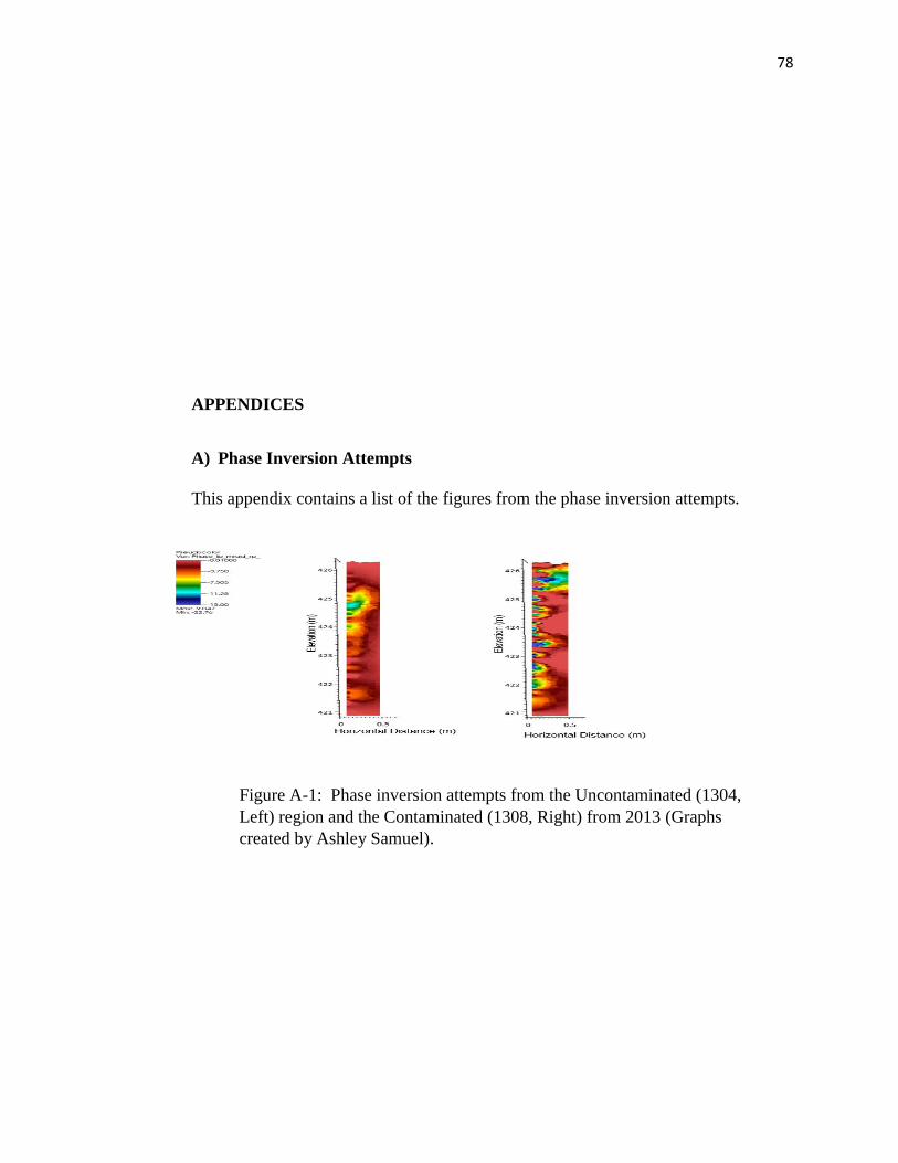
78

APPENDICES

A) Phase Inversion Attempts

This appendix contains a list of the figures from the phase inversion attempts.

Figure A-1: Phase inversion attempts from the Uncontaminated (1304,

Left) region and the Contaminated (1308, Right) from 2013 (Graphs

created by Ashley Samuel).

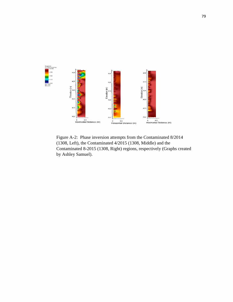
79

Figure A-2: Phase inversion attempts from the Contaminated 8/2014

(1308, Left), the Contaminated 4/2015 (1308, Middle) and the

Contaminated 8-2015 (1308, Right) regions, respectively (Graphs created

by Ashley Samuel).

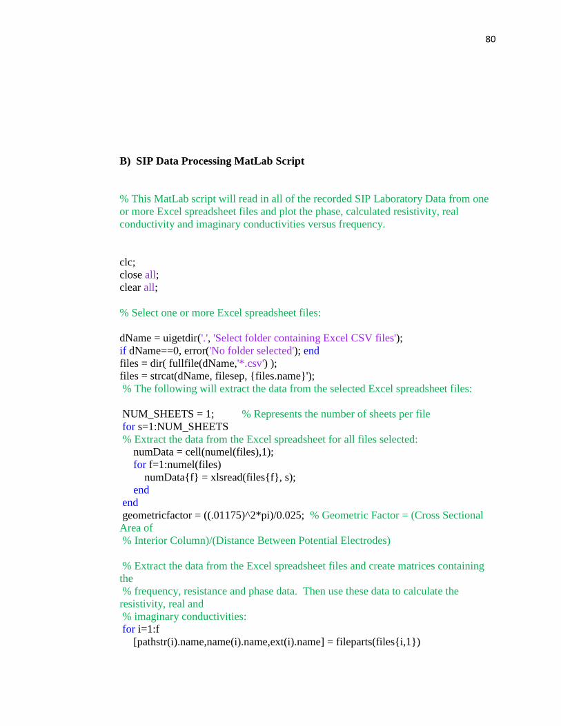
80

B) SIP Data Processing MatLab Script

% This MatLab script will read in all of the recorded SIP Laboratory Data from one

or more Excel spreadsheet files and plot the phase, calculated resistivity, real

conductivity and imaginary conductivities versus frequency.

clc;

close all;

clear all;

% Select one or more Excel spreadsheet files:

dName = uigetdir('.', 'Select folder containing Excel CSV files');

if dName==0, error('No folder selected'); end

files = dir( fullfile(dName,'*.csv') );

files = strcat(dName, filesep, {files.name}');

% The following will extract the data from the selected Excel spreadsheet files:

NUM_SHEETS = 1; % Represents the number of sheets per file

for s=1:NUM_SHEETS

% Extract the data from the Excel spreadsheet for all files selected:

numData = cell(numel(files),1);

for f=1:numel(files)

numData{f} = xlsread(files{f}, s);

end

end

geometricfactor = ((.01175)^2*pi)/0.025; % Geometric Factor = (Cross Sectional

Area of

% Interior Column)/(Distance Between Potential Electrodes)

% Extract the data from the Excel spreadsheet files and create matrices containing

the

% frequency, resistance and phase data. Then use these data to calculate the

resistivity, real and

% imaginary conductivities:

for i=1:f

[pathstr(i).name,name(i).name,ext(i).name] = fileparts(files{i,1})

81

Freq(i).name= numData{i,1}(16:52,2)

ResisMag(i).name = numData{i,1}(16:52,3) % This is really the Relative

Resistance

Phase(i).name = numData{i,1}(16:52,4) % Phase is in radians

resistance(i).name = 100*(ResisMag(i).name) % Resistance = 100*(Relative

Resistance)

resistivity(i).name = geometricfactor*resistance(i).name

% Resistivity = (Geometric Factor)*(Resistance)

Phaseforplotting(i).name = Phase(i).name*(-1)

% Phase = (Phase)* (-1) for plotting on positive y-axis

imaginaryconductivity(i).name= (((1./(resistivity(i).name))).*(-

1*sin(Phase(i).name)))

% Imaginary Conductivity = (1/Resistivity)*(sin(Phase))

realconductivity(i).name = (((1./(resistivity(i).name))).*(cos(Phase(i).name)))

% Real Conductivity = (1/Resistivity)*cos(Phase)

% Now to plot everything

figure(1)

cc=hsv(6)

subplot(2,2,1)

% This will plot the Phase versus Frequency:

semilogx(Freq(i).name, Phaseforplotting(i).name, '-o',

'MarkerEdgeColor', 'b', 'MarkerFaceColor', cc(i,:))

title('Phase vs. Frequency')

xlabel('Frequency (Hz)')

ylabel('Phase (radians)')

hold on

% This will plot the Resistivity versus Frequency:

subplot(2,2,2)

loglog(Freq(i).name,resistivity(i).name, '-

o','MarkerEdgeColor','b','MarkerFaceColor', cc(i,:))

title('Resistivity vs. Frequency')

xlabel('Frequency (Hz)')

ylabel('Resistivity (Ohm-m)')

hold on

% This will plot the Real Conductivity versus Frequency:

subplot(2,2,3)

loglog(Freq(i).name,realconductivity(i).name,'-o', 'MarkerEdgeColor', 'b',

'MarkerFaceColor',

cc(i,:))

title('Real Conductivity vs. Frequency')

82

xlabel('Frequency (Hz)')

ylabel('Real Conductivity (S/m)')

hold on

% This will plot the Imaginary Conductivity versus Frequency:

subplot(2,2,4)

loglog(Freq(i).name,imaginaryconductivity(i).name, '-

o','MarkerEdgeColor','b','MarkerFaceColor', cc(i,:))

title('Imaginary Conductivity vs. Frequency')

xlabel('Frequency (Hz)')

ylabel('Imaginary Conductivity (S/m)')

hold on

end

% This will plot the legend with every Excel Spreadsheet filename selected for

plotting:

legend(name(1,1).name, name(1,2).name, name(1,3).name, name(1,4).name,

'Location',

'Northwest')