NCER Working Paper SeriesNCER Working Paper Series

Investigating the Relationship Between DSGE and SVAR Models

Adrian PaganAdrian Pagan Tim RobinsonTim Robinson

Working Paper #112Working Paper #112 May 2016May 2016

Investigating the Relationship BetweenDSGE and SVAR Models∗

Adrian Pagan and Tim Robinson †

Melbourne Institute of Applied Economic

and Social Research, University of Melbourne

May 18, 2016

Contents

1 Introduction 2

2 Truncation Bias: DSGE Model and Data for SVAR ContainI(0) Variables Only 52.1 Analysis . . . . . . . . . . . . . . . . . . . . . . . . . . . . . . 62.2 Illustration: A Simple Real Business Cycle Model . . . . . . . 82.3 Illustration: The Justiniano-Preston (2010) Model . . . . . . . 92.4 Illustration: The Smets and Wouters (2007) Model . . . . . . . 12

3 Truncation Bias: DSGEModel and Data Contain Co-integratedI(1) Variables 173.1 Analysis . . . . . . . . . . . . . . . . . . . . . . . . . . . . . . 173.2 Illustration: The An and Schorfheide (2007) Model . . . . . . 193.3 Illustration: The Erceg et. al (2005) Model . . . . . . . . . . . 20

∗We are grateful to Efrem Castelnuovo and Mariano Kulish for comments on an earlierversion of this paper.

†Research Supported by ARC Grant DP160102654.

1

4 Estimating C0 234.1 Analysis . . . . . . . . . . . . . . . . . . . . . . . . . . . . . . 234.2 Illustration: The External Sector of the Reserve Bank of Aus-

tralia’s Multi-Sector Model (MSM) . . . . . . . . . . . . . . . 244.3 Implications . . . . . . . . . . . . . . . . . . . . . . . . . . . . 274.4 Conclusion . . . . . . . . . . . . . . . . . . . . . . . . . . . . . 28

5 References 29

Abstract

DSGE models often contain variables for which data is not ob-served when estimating. Although DSGE models generally implythat there is a finite order SVAR in all the variables this may nolonger be true for SVARs just in observable variables, and so there isa VAR-truncation problem. The paper examines this issue. It looksat five different studies using DSGE models that appear in the liter-ature. Generally it emerges that the truncation issue is probably notthat important, except possibly in small open economy models withexternal debt. Even when there is no truncation problem in VARs(which control the dynamics) the structural impulse responses fromboth models may be different due to differing initial responses. It isshown that DSGE models incorporate some strong restrictions on thenature of SVAR models and these would need to employed for the twoapproaches to give the same initial estimates.

1 Introduction

The relative utility of DSGE models versus SVARs in macroeconomic re-search has been a question of some interest. Because DSGE models havea strong economic orientation this has generally been investigated by ask-ing whether the SVAR can capture the impulse responses of the shocks ina DSGE i.e. the DSGE model is taken to be a good representation of themacro economy and the issue becomes whether the SVAR can capture theresults found with the DSGE model. There are two aspects to this ques-tion. Designating the j period structural impulse responses from the DSGEmodel by CDSGE

j these are constructed recursively from the impact impulseresponses CDSGE

0 and the underlying VAR coefficients. This leads to therelation CDSGE

j = DDSGEj CDSGE

0 , where the DDSGEj are the responses of

2

variables to the underlying VAR ( reduced form) equation errors. There areequivalent measures for any SVAR model fitted to the data and these will bedesignated as CSV AR

0 and DSV ARj . For the SVAR to match the DSGE model

responses we will need CSV AR0 = CDSGE

0 and DSV ARj = DDSGE

j .

Now, although a DSGEmodel generally has a finite order VAR solution inall its variables, this may become an infinite order when only the observablevariables are included. Thus, because SVARs in the observable variablesmust be of finite order, there can be differences between DSV AR

j and DDSGEj .

So a primary question to settle is whether the DSGE model also has a finiteorder VAR representation in observable variables. If that is not true thena secondary question relates to the magnitude of the approximation errorin DSV AR

j i.e. how close are DSV ARj and DDSGE

j ? Once this is settled onecan turn to the question of whether CDSGE

0 = CSV AR0 and hence decide how

close the structural impulse responses CDSGEj and CSV AR

j are. Clearly thelast feature involves the ability to replicate the dynamics ( Dj) as well ascontemporaneous interactions ( C0).

Some of the work investigating this question has just proceeded by con-structing DSGE models and then looking at whether a finite order SVAR ofsome form can capture the impulse responses Cj from the DSGE model e.g.Chari et. al. (2005) and Christiano et. al. (2007) ( although both papersdo contain some analytic work on aspects of the issue). Chari et. al. sug-gested that SVARs could not capture what was in a DSGE while Christianoet. al. had a different position. Kapetanios et. al. (2007) also followedthis strategy, using a large DSGE model that was a miniature version of themodel used in the Bank of England in the 2000s. They assumed that CDSGE

0

was known and CSV AR0 was set equal to it, then finding that one needed

very high order VARs, as well as large numbers of observations, in order tocapture the correct DDSGE

j . This meant that there was a potential problemwith using a finite order SVAR ( now called a truncation issue). A number ofother authors have looked at this theoretically e.g. Fernandez-Villaverde et.al. (2007), Ravenna (2007) and Franchi and Vidotto (2013). In those papersrather complex conditions were established for the possibility of a finite orderSVAR to represent DSGE model responses. Giacomini (2013) gives a surveyof the area.

In this paper we return to the issue of "making a match" of the Cj betweenthe two vehicles for applied work. Section 2 establishes some conditions fora finite order VAR to capture the dynamics of the DSGE model in the casewhere variables in the latter are just I(0). These depend on the relationship

3

of observed and unobserved variables, specifically whether the unobservedvariables can be captured by the contemporaneous observed variables anda small number of their lags. Three examples are chosen to illustrate thepoints.

The first example given is of a basic RBC model with just a technologyshock. In this model the observed variable is a flow ( output) and the un-observed variable is a stock (capital). Its simplicity enables one to see theessential issues relating to approximation of the dynamics. Because mostSVARs are only formulated with flow variables, while DSGE models con-tain stocks as well, the question that naturally arises is what the impact ofomitting stock variables might be, and so the simple RBC model is a goodvehicle to examine this. In this context it is found that, although a very highorder AR in the flow variable (output) is needed to precisely capture theimpulse responses from the RBC model, even a very low order AR providesan excellent approximation.

The second example in section 2 uses a small open economy model. Againthere would be an unobserved stock variable, in this case the level of externaldebt. Unlike the omission of the stock variable in the simple RBCmodel case,impulse responses now differ substantially depending on whether the stockvariable is present in the SVAR. The reasons for this are discussed. Finally,the model in Smets and Wouters (2007) is examined. This has been used agood deal in research on the construction and estimation of DSGE models.Here the unobserved variables are two stocks of capital ( the actual valueand also that from a flex-price economy) and the price of capital. Liu andTheodoridis (2012, p.89) when working with this model found that " .. thetruncation bias is the dominant source of the bias in the estimated impulseresponse functions", and we show that this was due to the use of a monetarypolicy reaction function that depends upon quantities derived from the flex-price economy. There is a relatively small bias when monetary policy reactsto disequilibria in the actual economy rather than to that in the flex priceeconomy.

Section 3 moves on to the case where there is co-integration between I(1)variables in the DSGE model. In this instance the DSGE model implies aVECM structure with a latent factor driving the common permanent compo-nents. In such a case two problems can arise. The first is that investigatorswork with a VAR formulated in the differences of the I(1) variables. Thisis a specification error, as it ignores the fact that such variables are drivenby latent error correction (EC) processes. A correction can be made for this

4

error by estimating a latent factor VECM process rather than a VAR in thechanges in the I(1) variables. A second problem is the one encountered in sec-tion 2 i.e. the presence of unobserved stock variables. We look at two modelsthat exhibit one or both of these issues. These are by An and Schorfheide(2007) and Erceg et. al. (2005). Erceg et. al. found that a finite order VARcould recover impulse responses accurately when the model they used hadan RBC orientation, but not when non-neutralities are introduced, and weexplain why this is so.

As already intimated a good approximation of theDSV ARj to theDDSGE

j isonly one aspect of the problem of matching the structural impulse responsesfrom SVAR and DSGE models. In many instances it is a gap between CSV AR

0

and CDSGE0 that creates the matching problems, and so we need to look at

whether the C0 implied by a DSGE model can be captured by a SVAR.Effectively, this is a question about the definition of structural shocks ratherthen their dynamic effects. If C0 is known to be that implied by the DSGEmodel then the shocks are defined properly and incorrect impulse responsessimply reflect the truncation issues with a VAR. Fundamentally, the difficultyis that researchers work with SVARs so as to have a great deal of flexibilityin dynamics and this creates identification problems when trying to estimateC0. We analyze these in section 4 and suggest some responses for appliedwork. Section 5 concludes.

2 Truncation Bias: DSGE Model and Data

for SVAR Contain I(0) Variables Only

We initially provide some analysis of this in terms of the conditions neededfor a finite order VAR in observables to come from a VAR in both observableand unobservable variables. Then we look at this condition in some DSGEmodels. It is assumed that there is a VAR of order q in all variables impliedby the DSGE model. But when there are unobservables it may no longer bethe case that the order of the underlying VAR is finite. In contrast an SVARalways involves a finite order p. Hence we need to begin with an analysis ofhow the order of the DSGE-implied VAR changes when only observables areconsidered. We note that the responses to the VAR errors -Dj - would be

5

computed in both cases by

DDSGEj = BDSGE

1 DDSGEj−1 + ...+BDSGE

q DDSGEj−q ,DDSGE

0 = I

DSV ARj = BSV AR

1 DSV ARj−1 + ...+BSV AR

p DSV ARj−p , DSV AR

0 = I,

where Bj are the VAR coefficients for the system with variables zt i.e. zt =B1zt−1 + ...+Bq(p)zt−q(p) + et.

2.1 Analysis

Historically all variables in DSGE models were taken to be I(0) so we startwith an analysis of the VAR implied by DSGE models in such a case. Let ztbe the variables in a DSGE model. In most instances the DSGE model hasthe structural equations1

A0zt = CEt(zt+1) +A1zt−1 +Hut, (1)

where ut are shocks possibly following a VAR(1), ut = Φut−1 + εt, and εt isa vector of white noise processes with covariance matrix Ω that is diagonal.This system can then be solved for zt by using ( for example) the method ofundetermined coefficients. This produces a solution

zt = Bzt−1 +Gut.

Binder and Pesaran (1995) look at this. The conditions for the solution aretwofold: a rank condition and the Blanchard-Kahn stability conditions mustbe satisfied. Users of Dynare will be familiar with the program checking theseconditions. In the case where the number of shocks is not greater than zt wecan write ut = G+(zt −Bzt−1). Thereupon, using ut = Φut−1 + εt yields

G+(zt −Bzt−1) = ΦG+(zt−1 −Bzt−2) + εt,

making the solution for zt a VAR(2). This was done in Kapetanios et. al.(2007) and Ravenna (2007).

The problem in practice is that not all of the zt are observable and atraditional VAR requires that one work with observable variables. Hence we

1There are very few DSGE models that cannot be written in this way. If the modelequations in (1) involve more than one lag in variables then we would need to expand ztto contain lagged variables. The analysis would still proceed in the same way but it wouldbe necessary to select the current values of variables from the augmented zt vector.

6

have to allow for the fact that there are two types of variables in zt - observedzot and unobserved zut . In this case the solved VAR can be decomposed as 2

zot = Aoozot−1 +Aouz

ut−1 +Gout

zut = Auozot−1 +Auuz

ut−1 +Guut.

Now in most DSGE models the number of shocks equals the number ofobserved variables. In that case

ut = G−1o (z

ot − Aooz

ot−1 −Aouz

ut−1),

and so

zut = Auozot−1 +Auuz

ut−1 +GuG

−1o (z

ot − Aooz

ot−1 −Aouz

ut−1)

= GuG−1o zot + (Auo −GuG

−1o Aoo)z

ot−1 + (Auu −GuG

−1o Aou)z

ut−1

= F1zot + F2z

ot−1 + F3z

ut−1

=⇒ zut = (I − F3L)−1F1z

ot + F2z

ot−1,

and it is possible to recover the unobservables from the observables using thecontemporaneous values and enough lags of the latter. Hence the VAR inobservable variables will be

zot = Aoozot−1 +Aou(I − F3L)

−1F1zot−1 + F2z

ot−2+Gout, (2)

and we see that this will generally not produce a finite order VAR in observ-ables zot i.e. the DSGE model will have an underlying VAR of order q =∞.

For it to be finite we would need either F3 = (Auu − GuG−1o Aou) = 0 i.e.

Auu = 0, Aou = 0 or Auu = 0, Gu = 0. However, it should be noted that,if F1, F2 and Aou are small, then the higher order terms introduced into theVAR owing to the need to eliminate the unobservables will add very little tothe simple finite order VAR. One way of thinking about this is to ask whetherwe can recover zut by regressing it upon z0t−j

Kj=1 and how many lags (K)

would it take to produce a perfect fit?That there may be problems coming from unobservables in SVARs arises

from the fact that SVARs are mostly formulated in flow variables while there

2Note that we have not solved for the complete VAR as the error term in this form isut and not εt. But as shown previously converting to a VAR that has εt just raises theorder by one, so it is simplest to do the analysis using the form with ut.

7

are stock variables in many DSGE models. Perhaps the most obvious ex-ample of this is the presence of a capital stock in DSGE models. Theevolution of capital stock, in log linearized form, would be described bykt = (1 − δ)kt−1 + δit, resulting in the relevant element in Gu being zero.However, that in Auu is not zero, meaning that the missing capital stockwould need to be inferred from the observable variables in a VAR. In manyinstances though the unobserved variables can be expressed as a function ofa finite number of observed variables and their lags and hence the VAR re-mains of finite order. This latter condition is basically that found by Franchiand Vidotto (2013) (as shown by them in an appendix) and also by Fukacand Pagan (2007).

2.2 Illustration: A Simple Real Business Cycle Model

To look at the results mentioned above suppose we take the basic RBCmodel in Uhlig (1999) which has the equations ( where investment has beensubstituted out)

lt = yt − ct (3)

C∗

Y ∗ct +

K∗

Y ∗kt = yt + (1− δ)

K∗

Y ∗kt−1 (4)

ct = Et(ct+1 + rt+1) (5)

R∗rt = αY ∗

K∗(yt − kt−1) (6)

yt = (1− α)at + αkt−1 + (1− α)lt (7)

at = ρaat−1 + εat . (8)

Here small letters represent log deviations from steady state, * are steadystate values, ct is consumption, kt is the capital stock, rt is the gross realrate of return, at is an AR(1) technology shock with parameter ρa, and lt islabour input. The parameters are set to α = .4, δ = .025, ρa = .9, R∗ = .99,and the steady state values are functions of these parameters. The solutionfor output will be yt = .133kt−1 + 1.21at ( this comes from Dynare’s "Policyand Transition Functions"). The same expression for capital is kt = .95kt−1+.094at.

Now yt is the observed variable and kt the unobserved one. Hence, toevaluate the adequacy of an AR process for capturing the DSGE implied

8

VAR we would have Auu = .95, Aou = .133, Gu = .094, Go = 1.21, leadingto F1 = .0777, F2 = 0, Aou = .133 and F3 = .94. This value for F3 suggeststhat extraction of a good measure of the capital stock from output datawould require many lags of that variable. However, if one considers what theAR equation for yt is (after eliminating kt) we would get

yt = Aou(I − F3L)−1F1yt−1 = .133× .0777×

∞

j=0

(.94)jyt−1−j + 1.21at

= .01yt−1 + .001yt−2 + ...+ at,

so that the AR process for yt will be approximately

yt = .91yt−1 + 1.21εat .

Hence, even an AR(1) in yt will capture the RBC model impulse responsesvery well.3 Thus, whilst it is important to look at the roots of F3, it is thecase that even very high values of those do not preclude a low order VARproviding a good approximation to that of the DSGE model i.e. DDSGE

j andDSV ARj can be close.

2.3 Illustration: The Justiniano-Preston (2010) Model

This model is a small open economy model that has more than twenty en-dogenous variables and eight shocks including technology, preferences andrisk. Eight variables were taken to be observable - domestic output, an in-terest rate and inflation ( yt, it and πt respectively), the same for foreignvariables ( y∗t , i

∗

t and π∗t ), and the nominal and real exchange rates (st andqt). Its solution is a VAR(2). An example of one of the VAR(2) equations(that for output) follows:4

3In fact yt is actually a ARMA(2,1) process of the form yt = 1.85yt−1 − .855yt−2 +1.21εt − 1.138εt−1 and there are close to cancellation of the roots of the polynomials(1− 1.85L+ .855L2) and (1.21-1.138L).

4This equation is an identity, as shown by the expression for the VAR error eyt interms of the structural shocks εt. In all the work of this paper data was simulated fromthe models and then the identity governing the evolution of variables was found by fittinga regression. Because the VAR errors are irrelevant for discussing dynamics i.e. estimatingDj , we will leave them out when writing down the identities in the remaining section ofthis paper. When we return to estimating C0 in the next section we will provide thecomplete identities as the shocks are crucial to C0.

9

yt = 1.02yt−1 − .18yt−2 − .045y∗t−2 +−.005i∗

t−1 + .033π∗t−1 + .023it−1 − (9)

.017qt−1 + .028qt−2 − .34πt−1 + .017πt−2 − .001Dt−1 − .017mct−1 + eyt

eyt = .05εgt + .15εat − .12εcft − .36εrt + .43εrpt + .21εy∗

t + .05επ∗

t − .27εr∗

t (10)

There are clearly quite a few unobserved variables in the complete system,but, as the identity shows, these substitute out, leaving only two that areunobserved and which enter the VAR equation above - the net foreign assetposition ( Dt) and the level of marginal costs (mct). Computing F3 for thesystem ( where Dt is the first unobserved variable) we get

F3 =

.994 −.001735.1976 −.005883

,

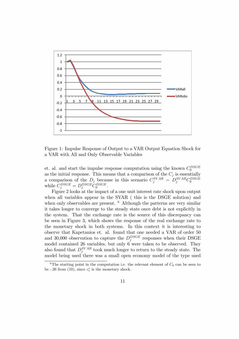
with eigenvalues of .9937 and -.0055. This points to the possibility that theomission of the stock variable Dt from the VAR might be important. Wenote that, just as for the RBC model, the omitted stock variable is verypersistent. In fact it is far more persistent than for the capital stock in thatmodel. Consequently, Figure 1 looks at the responses of yt to the error inthe VAR equation for yt when (a) The VAR contains all ten variables and(b) The VAR has just the eight observable variables.

For about six quarters the responses to the VAR output equation errorfor both the DSGE and SVAR models are reasonably close, but then theybegin to deviate. The complete system returns to the steady state positionmuch faster with the "all variables" VAR than for a VAR which omits foreignasset balances and marginal costs. The logic is that the accumulation of debtis important for driving up the risk premium in the DSGE model (and hencethe exchange rate), and this will be a stabilizing mechanism present in the"all variable" VAR that is much more weakly present in the VAR based ononly observed variables.5 That this is a strong mechanism can be seen fromthe mapping between Dt and current information, available from the identity

Dt = 1.01Dt−1 − .388889(y − y∗t ) + .147156 ∗ s− .054444qt.

Another view of this is to be had by computing the impulse functions to amonetary shock in both the DSGE and SVAR models. We follow Kapetanios

5Schmitt-Grohe and Uribe (2003) discuss a variety of methods for inducing a stabilizingmechanism into open economy models, of which this is one.

10

-1

-0.8

-0.6

-0.4

-0.2

0

0.2

0.4

0.6

0.8

1

1.2

1 3 5 7 9 11 13 15 17 19 21 23 25 27 29

VARall

VARobs

Figure 1: Impulse Response of Output to a VAR Output Equation Shock fora VAR with All and Only Observable Variables

et. al. and start the impulse response computation using the known CDSGE0

as the initial response. This means that a comparison of the Cj is essentiallya comparison of the Dj because in this scenario CSV AR

j = DSV ARj CDSGE

0

while CDSGEj = DDSGE

j CDSGE0 .

Figure 2 looks at the impact of a one unit interest rate shock upon outputwhen all variables appear in the SVAR ( this is the DSGE solution) andwhen only observables are present. 6 Although the patterns are very similarit takes longer to converge to the steady state once debt is not explicitly inthe system. That the exchange rate is the source of this discrepancy canbe seen in Figure 3, which shows the response of the real exchange rate tothe monetary shock in both systems. In this context it is interesting toobserve that Kapetanios et. al. found that one needed a VAR of order 50and 30,000 observation to capture the DDSGE

j responses when their DSGEmodel contained 26 variables, but only 6 were taken to be observed. Theyalso found that DSV AR

j took much longer to return to the steady state. Themodel being used there was a small open economy model of the type used

6The starting point in the computation i.e. the relevant element of C0 can be seen tobe -.36 from (10), since εrt is the monetary shock.

11

-0.4

-0.35

-0.3

-0.25

-0.2

-0.15

-0.1

-0.05

0

1 4 7 10131619 22 25 2831 34 37 40 434649525558

y/monobs

y/monall

Figure 2: Response of Output to a One Unit Interest Rate Shock for theDSGE model ( SVAR with all variables) and for a SVAR With Just Observ-ables

by Justiniano and Preston. This suggests that the level of debt in SVARsof small open economies may be an issue in getting a correct measure of thedynamics, as seen through Dj .

2.4 Illustration: The Smets andWouters (2007) Model

The Smets and Wouters (2007) (SW) model provides some extra insight intothe relationships. This is a model that has a large number of variables (twenty four) but only seven shocks and observable variables. In its originalform the marginal cost shocks are ARMA processes so, by definition, thesolution will not involve a finite order VAR. However, in this section wereplace those ARMA terms with standard AR processes. Then the SWmodelcomes down to solving a VAR(2) in ten variables. Of these ten variablesseven are directly observable - logs of output yt, consumption ct, investmentit, hours ht, inflation πt, wages wt and the the interest rate rt. This leavesthree unobserved variables - capital kt, the flex-price level of capital kft, and

12

-0.8

-0.7

-0.6

-0.5

-0.4

-0.3

-0.2

-0.1

0

1 4 7 10 13 16 19 22 25 28 31 34 37 40 43 46 49 52 55 58

q/monall

q/monobs

Figure 3: Response of the Real Exchange to a One Unit Interest Rate Shockfor the DSGE model ( SVAR with all variables) and for a SVAR With JustObservables

13

the price of capital pkt. Of the original twenty four variables fourteen areunobserved and these are essentially substituted out using identities. TheF3 matrix investigated earlier is

F3 =

.97 0 0.05 .97 .14−.32 −.009 .744

,

with eigenvalues of .97, .96 and .75. This points to possible issues for theorder of the VAR in observables.

To study this more closely consider the equation for yt from the SVAR(2).

yt = 1.74ct−1 − 1.47ct−2 − .04it−1 − .04it−2 − .09ht−1 − .001ht−2 + .649πt−1

−.3πt−2 + .72wt−1 − .52wt−2 − .47rt−1 + .21rt−2 + 1.06yt−1 + .0008yt−2

−.21kt−1 − .008kt−2 − .009kft−1 + .008kft−2 − .41pkt−1.

It is immediately clear that the system will not be a finite order VAR in termsof observable variables, and might require a high order VAR due to the largecoefficients on kt−1 and pkt−1. This is confirmed by looking at the responsesof yt to the VAR output equation error in Figure 4 i.e. the correspondingDj. The cases considered in this figure are where all variables are in theVAR, then kft is excluded ( in this instance it is almost impossible to seeany difference), kt is excluded and, finally, all of kt, kft and pkt are excluded.There is clearly a loss in accuracy for not having information on the capitalstock and the price of capital, although it is the latter which has the greatestimpact. It is apparent that the shape of the impulse responses are lost whenonly observables are used and the magnitudes are also an issue. This wasLiu and Konstantinos’ (2012) conclusion.

To explore these results further we note that the reason for kft appearingin the VAR is the fact that the interest rate rule in the SW model dependson (yt − yft). In many models this rule does not depend on the flex priceeconomy equilibrium output and instead is related directly to yt. Hence weconvert the SW model to one with such an interest rate rule. Then it turnsout there is just one unobservable - kt . Figure 5 shows the same type ofimpulse responses as in figure 4 ( except there is now only one unobserv-able, kt) with the addition of a new one. This new response is arrived atby computing a pseudo-value for the capital stock using investment and a

14

0

0.2

0.4

0.6

0.8

1

1.2

1.4

1.6

1 3 5 7 9 11 13 15 17 19 21 2325 27 29 31 33 35 37 39

allin

nok

nokf

onlyobserv

Figure 4: Impulse Responses of Output to the VAR Output Equation Shockfor Different VARs with Varying Unobservable Variables from the Smets-Wouters Model.

15

0

0.5

1

1.5

2

2.5

3

3.5

1 3 5 7 9 111315171921232527293133353739

VARobs/yVARall/y

VAR(2)all

VARconk/y

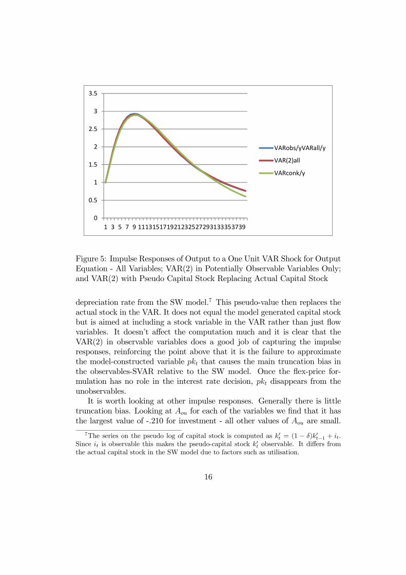
Figure 5: Impulse Responses of Output to a One Unit VAR Shock for OutputEquation - All Variables; VAR(2) in Potentially Observable Variables Only;and VAR(2) with Pseudo Capital Stock Replacing Actual Capital Stock

depreciation rate from the SW model.7 This pseudo-value then replaces theactual stock in the VAR. It does not equal the model generated capital stockbut is aimed at including a stock variable in the VAR rather than just flowvariables. It doesn’t affect the computation much and it is clear that theVAR(2) in observable variables does a good job of capturing the impulseresponses, reinforcing the point above that it is the failure to approximatethe model-constructed variable pkt that causes the main truncation bias inthe observables-SVAR relative to the SW model. Once the flex-price for-mulation has no role in the interest rate decision, pkt disappears from theunobservables.

It is worth looking at other impulse responses. Generally there is littletruncation bias. Looking at Aou for each of the variables we find that it hasthe largest value of -.210 for investment - all other values of Aou are small.

7The series on the pseudo log of capital stock is computed as k′t = (1 − δ)k′t−1 + it.Since it is observable this makes the pseudo-capital stock k′t observable. It differs fromthe actual capital stock in the SW model due to factors such as utilisation.

16

-0.5

0

0.5

1

1.5

2

2.5

3

3.5

4

4.5

1 3 5 7 9 111315171921232527293133353739

VARobs/inve

VARall/inve

VARconk/inve

Figure 6: Impulse Responses of Investment to a One Unit VAR Shock for theOutput Equation - All variables, VAR(2) in Potentially Observable VariablesOnly, and a VAR(2) with Pseudo Capital Stock replacing Actual CapitalStock

So this suggests that it may be the response of investment to VAR outputequation errors that is potentially subject to a bias. Accordingly, the impactof a unit rise in the VAR output equation error upon investment is presentedin Figure 6. Even in this case the bias is relatively small until after nine orso periods ahead. The pseudo-capital stock approach to correcting the biasworks very well for around 20 periods, but it becomes quite large after aboutthirty three periods.

3 Truncation Bias: DSGE Model and Data

Contain Co-integrated I(1) Variables

3.1 Analysis

Euler equations in DSGEmodels have a structure such asC−1t = βEtC

−1t+1Rt+1,

where Ct is the level of consumption and Rt is a real interest rate. When vari-

17

ables are stationary the equation can be re-expressed in terms of ratios to thesteady state positions C∗ and R∗ i.e. ( Ct

C∗)−1 = βR∗Et(

Ct+1C∗)−1Rt+1

R∗but, when

variables are I(1) and co-integrated, some other divisor has to be used. Tra-ditionally in DSGE models this has been the level of technology, so that theconsumption Euler equation becomes (Ct

At)−1 = βR∗Et(

Ct+1At+1

)−1(At+1At)−1Rt+1

R∗.

Then, after log-linearization, this is

ct − at = Et[ct+1 − at+1 +∆at+1]−Etrt+1 + ln r∗,

where the lower case letters represent the logs of the upper case ones. Mostmodern DSGE models now have the log of technology ( at) being an exoge-nous I(1) process of the form

.∆at = ρa∆at−1 + εat.

This is particularly so for those models used in a policy environment.Under such a specification Et∆at+1 = ρa∆at, making the linearized con-

sumption Euler equation:

ct − at = Et[ct+1 − at+1] + ρa∆at −Etrt+1 + ln r∗.

Then ct − at is I(0). All the model variables which are I(1) are expressedas deviations from at, a process often referred to as "stationizing". Thus, interms of the RBC model of the previous section, if at was a unit root processwe would have variables yt − at, ct − at etc. These variables are then I(0)and represent the error correction (EC) terms. The consequence is that thereis co-integration between the three variables yt, ct, and at. These EC termswould be present among the zt of the previous section and, after the DSGEmodel is solved (as outlined earlier), there will be a VAR in the zt.

Now just as before there will be observed and unobserved variables amongthe zt. First, we note that the "stationized" variables yt− at etc., designatedwith a superscript S, are not directly observed data, but they generally re-late to observed data. Specifically, with ∆ct being the observed data onconsumption growth,

∆ct = ∆(ct − at) + ∆at = ∆cSt +∆at.

In contrast there can be some other stationized variables that do not relatedirectly to data and which require a model for their construction e.g. thecapital stock. With the first type of variable it is necessary to add a statisticalspecification for the latent exogenous process at, but we do not need aneconomic model for that.

18

3.2 Illustration: The An and Schorfheide (2007) Model

Now consider models in which there is an I(1) process for at and some I(1)variables that are stationized. To fix the ideas, it helps to discuss a modelthat has been a work horse for analysis. Specifically we take the An andSchorfheide (2007) model that has been analyzed in Giacomini (2013). Hereyt is the log of output, ct is the log of consumption, πt is the rate of inflation,rt is the interest rate and gt is a fiscal variable. The technology shock isεa,t, the fiscal shock is εg,t and the monetary shock is εr,t. The model has theequations:.

ySt = Et(ySt+1) + gt −Etgt+1 −

1

τ(rt −Etπt+1 − Et∆at+1)

πt = βEt(πt+1) +τ (1− ν)

π2φ(ySt − gt)

cSt = ySt − gt

rt = ρrrt−1 + (1− ρr)ψ1πt + (1− ρτ )ψ2(ySt − gt) + ρrεr,t

∆at = ρa∆at−1 + σaεa,t

gt = ρggt−1 + σgεg,t

ySt = yt − at.

It is clear that there is co-integration between yt, ct and at. Given shocksgt,∆at and εrt it is possible to solve the system for ySt , πt and rt, and thesolution for cSt would then follow from the identity relating ySt and gt. Giventhe parameter values in Giacomini (2013) the numerical solution for thissystem is

ySt = .95ySt−1 − .5πt−1 + .1945rt−1 + .0037εat + .006εgt − .0019εrtπt = .616πt−1 − .114rt−1 + .0037εat − .0012εrtrt = .776rt−1 + .308πt−1 + .0018εat + .0013εrt .

Hence, as pointed out in Giacomini, the solution is a finite order VAR inySt , πt and rt. However this involves the unobservable ySt and so this is notstrictly an observables-VAR. The latter would have to be in terms of ∆yt, πtand rt.

Due to the relation∆yt = ∆ySt +∆at, (11)

19

the equation for growth in output that would define the observable systemwill be

∆yt = −.05ySt−1 − .5πt−1 + .1945rt−1 +∆at + .0037εat + .006εgt − .0019εrt ,

that is, it is an equation from a Vector Error Correction Model (VECM) thathas ySt−1 as the lagged error correction term. But, if the system is expressedas a VAR in observables, then the term −.05ySt−1 would be ignored. Thusthis would be a specification error and would result in there being a VARMArather than a VAR structure.8 How important the MA component will bedepends on the relative variances of −.05ySt−1 and ∆at + .0037εat + .006εgt −.0019εrt . Figure 7 shows the responses of ∆yt to the error in the VAR equationfor yt from the An and Schorfheide model as the order of the VAR increases.It demonstrates that very high order VARs would be needed to fully capturethe impulse responses.

It should be emphasized here that we are really dealing with a VECMmodel in terms of ∆yt, ∆at and yt − at as the error correction term. Itis because a VAR formulated in just ∆yt, πt and rt ignores the EC termthat a truncation bias emerges. But this can be simply avoided by fitting afinite order latent factor VECM which includes ySt−1 in the ∆yt equation. Inorder to perform the estimation of such a system all that is required is somestatistical assumption about the nature of ∆at. The latter is an exogenousitem to the DSGE model as well. One can estimate latent factor VECMs ofthis form easily in Dynare and, indeed, any DSGE model with I(1) variablesis essentially being estimated as a latent factor VECM.

3.3 Illustration: The Erceg et. al (2005) Model

Erceg et. al. (2005) have two different models. The first is what they call theRBC version and they find that the VAR representation exhibits very littletruncation error. The second which involves nominal rigidities is different.

8This points to the fact that a VAR in observable variables will rarely be the appropriateway to proceed if data is generated by a DSGE model with non-stationary technology. Ifone thought of the SW model as having a unit root in technology then there would bestationized variables such as (yt − at), (ct − at), (it − at) etc. These could be transformedto (ct−yt), (it−yt) and (yt−at), but there will always be one unobservable EC term thatwould be missing from an observables-VECM.

20

-0.06

-0.05

-0.04

-0.03

-0.02

-0.01

0

0.01

1 2 3 4 5 6 7 8 9

var1y/y

var4y/4

var20y/y

var100y/y

var200y/y

Figure 7: Impulse Responses of Output to the VAR Output Equation Shockfor Different Order VARs in ∆yt, πt and rt

For the first model they fit a four variable VAR to the simulated DSGEmodeldata and find a good approximation to the DSGE model impulse responses toa technology shock ( which is their main interest). There are four structuralshocks in this model and four observable variables - labour productivity lpt,

the log of the consumption to income ratio cyt, the log of the investment toincome ratio iyt, and hours worked ht. It turns out that the VAR implied bythe DSGE model has the exact form9

lpSt = 1.045lpSt−1 − .04cyt−1 + .034iyt−1 − .011ht−1

cyt = .08lpSt−1 − .926cyt−1 + .039iyt−1 − .02ht−1

iyt = −.22lpSt−1 − .143cyt−1 + .875iyt−1 − .05ht−1

ht = −.173lpSt−1 + .116cyt−1 − .075iyt−1 + 1.033ht−1.

So a finite order VAR in lpSt , cyt, iyt and ht fits exactly. Moreover, if oneadjoins the observation equation ∆lpt = ∆lp

St + ∆at, then we can estimate

9Again we have omitted the combination of white noise structural shocks that appearin the identities describing these equation since our focus is on Dj and not C0.

21

the system exactly using a latent variable VECM specification, thus avoidingany truncation bias. Hence, it is never appropriate in these cases to workwith a VAR in ∆yt.

10 It is interesting to note that, unlike the RBC modelof section 2, the capital stock can be substituted out using the identity kt =ht+ .024iyt+2.81lpt i.e. the assumption that labour productivity and hoursare known provides the necessary information. If instead one used ∆lpt inan observables-VAR then the approximation error will depend on the sizeof .045lpSt−1 to the shocks in the ∆lpt equation. The standard deviation ofthe former relative to the latter is about 1

14, so the use of the observables-

VAR rather than the latent VECM is likely to show up only in long horizonimpulse responses.

The second model that Erceg et. al. use has non-neutralities. A com-plication now is that there are five shocks but only the same number ofobservables as in the RBC model. This seems a little odd because thereis a monetary shock, so one might expect the interest rate to be added tothe VAR. The reason this matters can be seen from looking at the labourproductivity VAR equation for this model versus what it was for the RBCmodel

lpSt = .46lpSt−1 − .57lpSt−2 − 1.25cyt−1 + .63cyt−2 + .36iyt−1

−.34iyt−2 + .1ht−1 + .29ht−2 + .003kSt−1 − .95rt−1.

Here kt is the capital stock and rt is the interest rate. These can not besubstituted out and, since they are unobserved, there is no longer a finiteorder VAR in terms of lpSt etc. It may be that one can ignore the effects ofomitting the capital stock as its coefficient is quite small, but that on theinterest rate is large and its omission from the set of observables would likelymean truncation bias, which was found by Erceg et. al.

10In fact if one does so then all of the structural shocks would have permanent effectsupon yt and this would be contrary to what the DSGE model would say about them - seeFisher et. al (2016).

22

4 Estimating C0

4.1 Analysis

We now turn to an analysis of whether CSV AR0 relates closely to CDSGE

0 . Thisis a key element in describing the levels of impulse responses. In Figures 2and 3 we made these equal but, if they are not, then the responses wouldoriginate at different points, even though they would retain the same shape( as that comes from Dj). Theoretical models like DSGE have some of theirstructural equations with the form

z1t = φz1t−1 + ψEtz1t+1 + δz2t + ut,

where ut may be an AR(1) process. The complete system solves to bea VAR(1) or VAR(2) depending on whether there are AR(1) shocks andwhether φ = 0. The question then is what does this imply about SVARs? Itis useful to start the discussion by assuming that φ = 0, ut is an AR(1), andthe system solves to be a VAR(1).

Suppose a 3 variable structural system containing the equation above.The VAR(1) solution under the conditions just set out implies

z1t = b111z1t−1 + b112z2t−1 + b113z3t−1 + e1t, (12)

where e1t is a white noise VAR error. Then

Etz1t+1 = b111z1t + b112z2t + b113z3t.

Eliminating expectations the structural equation becomes

z1t = ψ(b111z1t + b112z2t + b113z3t) + δz2t + ut,

which can be written as

(1− ψb111)z1t = (ψb112 + δ)z2t + ψb113z3t + ut.

Gathering terms we get

z1t = a012z2t + a013z3t + u′t

a012 =ψb112 + δ

(1− ψb111), a013 =

ψb113(1− ψb111)

, u′t =ut

(1− ψb111).

23

This equation is the type of structural equation appearing in an SVAR.Notice that the coefficient a012 can be quite different to δ because it measuresnot just the direct response of z1t to variations in z2t but also the indirectresponses through variation in expectations. Thus if (12) was a standardPhillips curve in an NK model we would have z1t as the inflation rate and z2tas the output gap. The coefficient on the output gap in the SVAR equation

for inflation will be a012 =βb112+δ

(1−βb111), where β is the discount factor. Now if

there is a lot of persistence in inflation b111 will be close to unity and so a012may be many times larger than δ. In a typical NK model δ might be between.2 and .4 but, if say βb111 = .9, we see that the coefficient on the output gapfor a Phillips curve in an SVAR would lie between 2 and 4.

4.2 Illustration: The External Sector of the ReserveBank of Australia’s Multi-Sector Model (MSM)

A concrete example of this approach involves the equations of the externalsector of the Reserve Bank of Australia’s Multi-Sector Model (MSM) - Reeset. al. (2016). This is a small New Keynesian (NK) model of the form11

yt = Et(yt+1)− (rt − Et(πt+1)) + uyt (13)

πt = βEt(πt+1) + κyt + uπt (14)

rt = ρrrt−1 + (1− ρr)(γyyt + γππt) + δ∆yt + εrt, (15)

where uyt, uπt are AR(1) processes of the form

uyt = ρyuyt−1 + εyt

uπt = ρπuπt−1 + επt,

with εyt, εrπ, εrt being white noise processes that are uncorrelated with eachother. The NK model in (13)-(15) solves to gives a VAR(1) in yt, πt and rt.

Using the parameter values in Rees et. al. the VAR equations for yt andπt implied by (13)-(14) will be

11In this model yt is a stationized variable so a latent factor VECM would need to beused for estimation, as set out in the previous section. We abstract from that complicationhere and think of yt as being an observable output gap in order to make the points aboutestimating C0.

24

yt = .865yt−1 − .248πt−1 + .083rt−1 + .003εyt − .005επt − .049εrt

πt = .108yt−1 + .269πt−1 + .123rt−1 + .0006εyt + .013επt − .009εrt.

This gives us expressions for expectations of Etyt+1 = .865yt− .248πt+ .083rtand Etπt+1 = .108yt + .269πt + .123rt. So the Phillips curve will be

πt = β(.108yt + .269πt + .123rt) + κyt + uπt.

From Rees et.al. κ = .036, β = .9996, and the AR(1) for uπt is

uπt = .32uπt−1 + επt.

Hence

πt =.108β + κ

(1− .269β)yt +

.123β

(1− .269β)rt +

1

(1− .269β)uπt (16)

= .195yt + .168rt + 1.368uπt

= .195yt + .168rt + .32uπt−1 + .0207ηπt, (17)

where ηπt is white noise and has a variance of unity.As we have just seen the DSGE model implies an equation for πt of the

form in (17). This can be converted to a SVAR equation by multiplyingthrough by the polynomial in the lag operator (1-ρπL) ( ρπ = .32) to give

(1− ρπ)πt = .195(1− ρπL)yt + .168(1− ρπL)rt + .0207ηπt.

Hence the coefficients on πt−1, yt−1 and rt−1 all involve the same parameter ρπand there is a common factor (1−ρπL) in the three separate lag polynomialson πt, yt and rt. This COMFAC structure was investigated by Hendry andMizon (1978). Because of it there are only three coefficients that need tobe estimated in this equation - those for yt, rt and ρπ− and not the five ifthe dynamics in the equation were unrestricted. There are three instrumentsavailable to perform this estimation - πt−1, yt−1 and rt−1. So the SVAR modelis exactly identified. Estimating it with simulated data from the MSMmodel( 10000 observations) we get

πt = .192yt + .164rt + .31uπ,t−1 + .0028επ,t,

25

which provides an excellent match to the results in (17). Of course a lot of ob-servations are being used but, even when the sample is just 200 observations,we get

πt = .247yt + .227rt + .37uπ,t−1 + .0029επ,t.

So an IV estimator applied to the SVAR inflation equation would enableus to get close to that implied by the DSGE model. However traditionalSVAR work attempts to estimate an unrestricted SVAR(1) equation anddoes not impose the COMFAC restriction of the DSGE model. Some otherrestriction on this equation is then needed to get identification. Often thisinvolves setting one of the coefficients on yt or rt to zero so as to get arecursive model. The COMFAC restriction used in the MSM model (andDSGE models more generally) does not come from economic ideas but issimply a statistical assumption about the nature of shocks.

The output equation in the SVARwhich is derivable from the MSMmodelshows other aspects of the difficulty an SVAR will have in replicating the C0of a DSGE model. After substituting out the expectations it has the form

yt = .7716πt − 29.32rt + 1.7244uyt. (18)

Again the COMFAC restriction delivers enough instruments to estimate thisequation but parameter estimates of the SVAR found with 10000 simulatedobservations from the MSM model are

yt = .3976πt + 19.27rt + .824uyt−1 + εyt,

which is a very poor match to what the DSGE model predicts this equationwould be. The reason is simply that rt−1 is a very poor instrument and sothe model is essentially unidentified.

Of course the MSM structural equation for output doesn’t involve theestimation of any parameters ( excluding the shock variance) as the coefficienton the real interest rate is set to -1 and that on Et(yt+1) to unity. Suppose weimposed the latter and worked with an SVAR inflation equation that involveda real interest rate. Both expectations in this equation can be constructedwithout knowing the form of the structural relations by estimating the VARequations for πt and yt to get the predictions Et(yt+1) and Et(πt+1). Theresulting instrumental variable (IV) estimator is

ψt = yt − Et(yt+1) = −.917(rt − Et(πt+1)) + .953uyt−1 + εyt.

26

This is quite a good match (ρy = .95) to that implied by the DSGE model.With 200 observations one gets

yt = −.45(rt −Et(πt+1)) + .927uyt−1 + εyt.

Turning to the final equation in the MSM external system the SVARequation for rt from the DSGE model is

rt = .928rt−1 + .154yt − .139yt−1 + .107πt.

Now this equation could be estimated using the three available instru-ments yt−1, rt−1 and πt−1. But, even with 10000 observations, the point es-timates are very bad. There are no data transformations or a COMFACrestriction in this equation which might be used to improve the estimation.However, SVARs do use the assumption that the white noise shocks are un-correlated with one another, meaning that επt and εyt can be used as extrainstruments, if they can be constructed. To do so apply the restrictions dis-cussed above ( COMFAC plus parametric) to the SVAR inflation and outputequations to get the residuals επt and εyt. These can then be used as extrainstruments. Doing this IV estimation with the 10000 observation simulateddata set produces

rt = .928rt−1 + .150yt − .136yt−1 + .105πt,

which agrees very closely with the DSGE structural equation. When only200 observations are used the parameter estimates become

rt = .942rt−1 + .14yt − .116yt−1 + .078πt,

which still represents a good match. Thus, if one utilizes some of the keyrestrictions and parameterizations of DSGE models, it is possible for theSVAR to capture C0 reasonably well, even in relatively small samples.

4.3 Implications

As the analysis and illustration shows the difficulties that a SVAR can expe-rience in capturing the C0 from a DSGE model often stem from the fact thatthe traditional estimation of SVAR models seeks to avoid imposing statisticalrestrictions ( such as COMFAC), exclusion restrictions ( in the interest rateequation πt−1 does not appear), and other constraints where coefficients are

27

prescribed ( for example on Et(yt+1) in the output equation). It also becomesdifficult to impose quantitative parametric restrictions in the way that DSGEmodels do e.g. the DSGE model implies that the output SVAR equation (18)should have an interest rate coefficient of -29, far from the -1 of the DSGEoutput structural relation. This arises because of the presence of forward-looking expectations that are dated with information at t. If the informationwas dated at t− 1 then there would be no difference since expectations ap-pearing as Et−1(yt+1) would not induce contemporaneous terms such as ytand rt into the structural equation. So the difficulties of reconciling CDSGE

0

and CSV AR0 may often come from the dating of expectations. If the t-dating

of expectations is regarded as the most plausible then one has to be veryagnostic about the quantitative values of any SVAR coefficients. Of coursea SVAR could work with a series on t dated expectations by constructingthese from the underlying VAR, as seen in the previous sub-section. An em-pirical example of this is Catao and Pagan (2011), where incorporating theexpectations in this way led to what were called structured VARs. But thenwe have to know which equations have which expectations e.g. the Phillipscurve in the NK model does not involve an expectation relating to futureoutput, and the interest rate equation has no expectations.

In many ways SVARs are about assembling information concerning thedynamics and contemporaneous interactions between variables in the macro-economic system in such a way as to impose less structure than what formalmodels like DSGE do. Traditionally this flexibility has been achieved by usingexactly identified SVARs rather than the over-identified structural equationsof the DSGE approach. But to get exact identification does require someconstraints. One constraint that is common to both DSGE and SVAR mod-els is that the structural shocks are uncorrelated, and we saw that this wasimportant to exploit when estimating the interest rate rule of the MSM. An-other has been to make the SVAR recursive. Ideally this should stem fromgood institutional information, but often it is just a convenient assumptionrather than being judged plausible.

4.4 Conclusion

We have looked at the conditions whereby unobservables that appear inDSGE models can be expressed as a function of observables. If this functioninvolves only a finite number of lags of the observed variables then a finiteorder VAR can potentially capture impulse responses from a DSGE model.

28

Provided the weights on higher order lags of observables are low it still maybe possible to approximate the responses well with a finite order VAR. A sim-ple RBC model showed this. A small open economy model showed that theomission of the stock of debt from a VAR could result in truncation biases,although even then this was an issue only at longer horizon responses.

Turning to DSGE models with I(1) variables it was found that some ofthe truncation biases came from a mis-specification. The actual generatingprocess is a latent factor VECM and not a VAR in terms of observed quan-tities such as the growth in I(1) variables. Such a model is relatively easyto estimate and can be implemented so as to safeguard against truncationbias. Nevertheless, such a strategy does not overcome the potential prob-lems that arise from the omission of stocks. Prima facie this seemed to bean issue in connection with the well-known Smets-Wouters model. On closerexamination however it was found that the major truncation problem camenot from the lack of a stock of capital variable in the VAR, but rather amodel-constructed price of capital. This arose due to an interest rate rulein the Smets-Wouters model being dependent on quantities from a flex-priceeconomy that was defined by the model. When the interest rate rule wasmodified there was a relatively small truncation bias in the VAR. Thus weare led to think that the biggest issue in connecting SVAR and DSGE modelsis how one can capture the initial impulse responses ( C0) rather than thedynamics. It was shown that one might be able to provide a match betweenthe C0 from a SVAR with that from a DSGE model by using some of thefeatures of the latter, such as COMFAC and exclusion restrictions. In doingso though one would be taking away one of the attractive features of SVARwork, which is to make as few assumptions as possible in order to give somedata-based evidence on the behaviour of the macroeconomic system.

5 References

An,S. and F. Schorfheide (2007), "Bayesian Analysis of DSGE Models,"Econometric Reviews, 26, 113-172.

Binder,M and M.H.. Pesaran (1995), “Multivariate Rational Expecta-tions Models and Macroeconomic Modelling: A Review and Some New Re-sults” in M.H. Pesaran and M Wickens (eds) Handbook of Applied Econo-metrics: Macroeconomics, Basil Blackwell, Oxford.

Catao, L. and A. Pagan , “The Credit Channel and Monetary Transmis-

29

sion in Brazil and Chile: A Structured VAR Approach” L.F. Cespedes, R.Chang and D. Saravia (eds) Monetary Policy Under Financial Turbulence(Central Bank of Chile)

Chari, V.V., P.J. Kehoe and E.R McGrattan (2005), " A Critique ofStructural VARs Using Business Cycle Theory", Federal Reserve Bank ofMinneapolis Working Paper 631,

Christiano, L.J. and M. Eichenbaum and Robert Vigfusson (2007), "As-sessing Structural VARs," in: NBER Macroeconomics Annual 2006, Volume21, pages 1-106.

Erceg, C.J., L. Guerrieri and C. Gust ( 2005), "Can Long-Run Restric-tions Identify Technology Shocks?," Journal of the European Economic As-sociation, 3, 1237-1278.

Fernández-Villaverde, J., J.F. Rubio-Ramírez, T. J. Sargent and M. W.Watson (2007). "ABCs (and Ds) of Understanding VARs," American Eco-nomic Review, 97, 1021-1026.

Franchi, Massimo & Vidotto, Anna, 2013. "A check for finite order VARrepresentations of DSGE models," Economics Letters, Elsevier, vol. 120(1),pages 100-103.

Fukac, M. and A. R. Pagan “Commentary on ‘An Estimated DSGEModelfor the United Kingdom" Federal Reserve Bank of St Louis Review, 89, 233-240

Giacomini, R. (2013), "The relationship between VAR and DSGE mod-els", in T. B. Fomby, L. Kilian and A. Murphy (eds) VAR Models in Macro-economics — New Developments and Applications: Essays in Honor of Christo-

pher A. Sims, Advances in Econometrics, vol. 32, p 1-25.Fisher, L.A., H-S He and A.R. Pagan (2016), . "Econometric Methods

for Modelling Systems with a Mixture of I(1) and I(0) Variables", Journal ofApplied Econometrics ( forthcoming)

Hendry, D. F. and G. Mizon (1978). "Serial Correlation as a ConvenientSimplification, Not a Nuisance: A Comment on a Study of the Demand forMoney by the Bank of England," Economic Journal, 88, 549-63.

Justiniano, A. and B. Preston (2010). "Monetary policy and uncertaintyin an empirical small open-economy model," Journal of Applied Economet-rics, 25, 93-128.

Kapetanios,G. A.R. Pagan and A. Scott (2007) “Making a Match: Com-bining Theory and Evidence in Policy-oriented Macroeconomic Modeling”,Journal of Econometrics, 136, 505-594.

30

Liu, P. & T. Konstantinos ( 2012), "DSGE Model Restrictions for Struc-tural VAR Identification," International Journal of Central Banking,, 8, 61-95..

Ouliaris, S. and A.Pagan (2016) "A Method for Working With Sign Re-strictions in Structural Equation Modelling", Oxford Bulletin of Economicsand Statistics ( forthcoming)

Rees,D.M., P. Smith and J. Hall (2016), "A Multi-sector Model of theAustralian Economy", Economic Record (forthcoming)

Schmitt-Grohe, S and M. Uribe (2003). "Closing small open economymodels," Journal of International Economics, 61, 163-185.

Smets, F and R. Wouters (2007), "Shocks and frictions in US businesscycles: a Bayesian DSGE approach", American Economic Review, 97, 586-606.

Uhlig, H. (1999). “A Toolkit for Analysing Nonlinear Dynamic StochasticModels Easily”, in R. Marimon and A. Scott (eds), Computational Methodsfor the Study of Dynamic Economies, Oxford University, Press, 30-61

31