investigating the relationships between environmental stressors

Investigating the relationships between environmentalstressors and stream condition using Bayesian beliefnetworks

J . DAVID ALLAN*, LESTER L. YUAN †, PAUL BLACK ‡, TOM STOCKTON‡, PETER E. DAVIES § ,

REGINA H. MAGIEROWSKI§ AND STEVE M. READ–

*School of Natural Resources & Environment, University of Michigan, Ann Arbor, MI, U.S.A.†US Environmental Protection Agency, Office of Research and Development, National Center for Environmental Assessment, Washington,

DC, U.S.A.‡Neptune and Company, Inc., Lakewood, CO, U.S.A.§School of Zoology, University of Tasmania, Hobart, Tas., Australia–Forestry Tasmania, Hobart, Tas., Australia

SUMMARY

1. Stream reaches found to be impaired by physical, chemical or biological assessment generally

are associated with greater extent of urban and agricultural land uses, and lesser amount of

undeveloped lands. However, because stream condition commonly is influenced by multiple

stressors as well as underlying natural gradients, it can be difficult to establish mechanistic

relationships between altered land use and impaired stream condition.

2. This study explores the use of Bayesian belief networks (BBNs) to model presumed causal

relationships between stressors and response variables. A BBN depicts the chain of causal

relationships resulting in some outcome such as environmental impairment and can make use of

evidence from expert judgment as well as observational and experimental data.

3. Three case studies illustrate the flexibility of BBN models. Expert elicitation in a workshop

setting was employed to model the effects of sedimentation on benthic invertebrates. A second

example used empirical data to explore the influence of natural and anthropogenic gradients on

stream habitat in a highly agricultural watershed. The third application drew on several forms of

evidence to develop a decision support tool linking grazing and forestry practices to stream reach

condition.

4. Although data limitations challenge model development and our ability to narrow the range of

possible outcomes, model formulation forces participants to conceptualise causal mechanisms and

consider how to resolve data shortfalls. With sufficient effort and resources, models with greater

evidentiary strength from observational and experimental data may become practical tools to

guide management decisions.

5. Such models may be used to explore possible outcomes associated with a range of scenarios,

thus benefiting management decision-making, and to improve insight into likely causal

relationships.

Keywords: Bayesian belief network, causal inference, multiple stressors, stream impairment, streammanagement

Introduction

Significant advances in the assessment of impaired

waterways over the past several decades have resulted

in extensive government-sponsored programmes to eval-

uate river condition at regional and national scales. With

the advent of large-scale monitoring, individual stream

reaches can be categorised on a continuum of poor to

Correspondence: J. David Allan, School of Natural Resources & Environment, University of Michigan, Ann Arbor, MI 48109, U.S.A.

E-mail: [email protected]

Freshwater Biology (2012), 57 (Suppl. 1), 58–73 doi:10.1111/j.1365-2427.2011.02683.x

58 � 2011 Blackwell Publishing Ltd

excellent condition, and whole regions can be compared

with regard to average level of impairment (e.g. Paulsen

et al., 2008; Davies et al., 2010). This information is crucial

to determining if regulatory standards are met, and

identifying locations where active management is needed

to counteract stressors and improve stream condition.

Diagnosis of cause of impairment obviously must

accompany assessment if restorative actions are to be

well focused. Although considerably less literature for-

mally addresses this issue, relative to the very substantial

literature on biological assessment, the need for diagnosis

has not gone unrecognized. U.S. EPA maintains an online

Causal Analysis ⁄Diagnosis Decision Identification System

intended to assist in the identification of stressors

responsible for impaired waters. There may be sufficient

information available on chemical and physical conditions

to strongly suggest cause of impairment, and indeed, the

cause may be obvious when there is a recognisable

contaminant source in an otherwise apparently pristine

landscape. Biological assessment data also can be mined

for further insights, as when the traits or tolerances of

particular species can be strongly associated with partic-

ular stressors (Yuan, 2004; Pollard & Yuan, 2010).

Often, however, identifying the cause of impairment is

challenging (Downes, 2010). Although many studies now

demonstrate that indicators of altered and disturbed

landscape are effective predictors of impaired stream

conditions, mechanisms of impairment may be difficult to

determine because of covariation between anthropogenic

influences and natural landscape gradients; the potential

for multiple, scale-dependent mechanisms; nonlinearities;

and possible legacy effects (Allan, 2004). A recurring theme

in reviews of the influence of land use upon river habitats and

biota by Allan (2004), Hughes, Wang & Seelbach (2006),

Johnson & Host (2010) and Steel et al. (2010) has been the need

for an improved understanding of mechanistic relationships.

Bayesian belief networks (BBNs) offer a useful frame-

work to depict the chain of causal relationships resulting in

environmental impairment, and for quantifying the relative

influence of individual linkages with explicit uncertainty

(Borsuk, Stow & Reckhow, 2004). BBNs combine an

influence diagram that can be used to provide a visual

representation of the assumed cause and effect relation-

ships for the problem at hand, and a parent–daughter state

probability structure that quantifies pathway of influence.

Bayesian networks hold promise for predictions of

responses to multiple drivers, to identify key drivers, and

to guide management practices in real-world situations

through simulation and scenario modelling.

Visually, a Bayesian belief network (BBN) is an influence

diagram depicting logical or causal relations among factors

that influence the likelihood of outcome states of some

parameter of interest, such as ecological condition or

species viability. Variables are represented as nodes, with

arrows depicting the direction of causation or association

(Jensen, 1996). Causation is considered to flow from a

‘parent’ node to a ‘child’ node and is unidirectional (Fig. 1).

The value of the variable represented by each node is

Precipitation

Flow

Macroinvertebrate community

Habitat structure

Watershed characteristics

Sediment

Channel structure

Riparian structure

Chemical stressors

Other sources

Land use

Fig. 1 A simple influence diagram for a stream

macroinvertebrate community.

Bayesian belief networks for stream condition 59

� 2011 Blackwell Publishing Ltd, Freshwater Biology, 57 (Suppl. 1), 58–73

expressed as a probability distribution, conditioned on the

values of parent nodes. In Fig. 1, the probability that stream

flow will be a particular value is influenced by land use,

precipitation and terrain. Once the model structure has

been defined, the effects of parent nodes on child nodes are

quantified from expert knowledge, statistical analysis of

existing data or other types of associations and evidence

(Korb & Nicholson, 2004; Pollino et al., 2007). For example,

the probability distribution for precipitation may be deter-

mined by an analysis of the past 20 years of summer

rainfall. Specification of the parameterized BBN is an

iterative process, allowing model structure to be modified

as it is developed.

Development of a BBN typically begins with the selection

of a problem of interest and a related conceptual model of

relationships between key drivers and responses at appro-

priate scales. Appropriate output variables are selected,

such as water quality or some biological indicator, followed

by specification of initial model structure, which is an

unparameterised causal network, from knowledge or data.

Interest in the use of BBNs for ecological modelling has

grown in recent years to include applications to a variety of

problems including fisheries assessment (Lee & Rieman,

1997; Kuikka et al., 1999), forest regeneration (Haas, Mow-

rer & Shepperd, 1994), habitat restoration (Rieman et al.,

2001) and emerging infectious diseases (Plowright et al.,

2008). Applications to aquatic ecosystems include eutro-

phication in the Neuse River estuary, North Carolina

(Borsuk et al., 2004), an ecological assessment of the impacts

of changed environmental conditions on native fish com-

munities in a catchment in Victoria, Australia (Pollino et al.,

2007) and to assist in prioritizing river restoration options in

response to changing flows and land use (Stewart-Koster

et al., 2005; Webb, Stewardson & Koster, 2010).

Although the use of BBNs to represent ecological

knowledge and uncertainty clearly is growing, their use is

still rare. The purpose of this study is to explore some

potential advantages and disadvantages of using BBNs to

improve understanding of causes of stream impairment in

order to support management decisions. We illustrate their

utility with three case studies: one developed using

knowledge elicitation to quantify a specific stressor–

response relationship, a second constructed with data from

a specific study area and a mixed model constructed with a

range of evidentiary sources and inferential strength.

Influence of sediments on low-gradient streams – an

expert elicitation example

Sedimentation was reported to be the second most

common cause of pollution in assessed rivers and streams

by the 1998 National Water Quality Inventory (U.S.

Environmental Protection Agency, 2000), affecting 31%

of those considered impaired. This case study was

undertaken to determine whether the information neces-

sary to specify a BBN describing the effect of sedimenta-

tion on macroinvertebrate populations could be elicited

from a group of stream ecologists with relevant experi-

ence, in collaboration with specialists in Bayesian model-

ling. To quantify this stressor–response relationship based

on expert judgment, a stream setting (a Midwestern, low-

gradient stream) and a type of impairment (introduction

of excess fine sediment) were specified along with the

relevant chemical, physical and biological aspects of the

ecosystem. The scale of influence was considered to be a

single riffle in two identical catchments, both originally

forested but with different disturbance histories of log-

ging and conversion to row crop agriculture, causing

sediment loads to vary across the catchments. The

ecologists then described how these factors were con-

nected, and were asked to predict quantitatively how

different attributes of the macroinvertebrate assemblage

would change in response to increased levels of fine

sediment, compared with the baseline condition.

The elicitation approach consisted of several steps,

including conditioning, model structuring and elicitation

of probabilistic relationships among variables. Condition-

ing, which refers to the development of a common

problem focus among domain experts, sharing of relevant

knowledge and introduction to Bayesian approaches,

occurred prior to meeting as a group, by email and a

conference call. This also facilitated initial model struc-

turing, which involved establishing assumptions and

conditions for the model as well as relationships between

variables. Several initial influence diagrams were dis-

cussed and revised, resulting in a preliminary influence

diagram of possible relationships between sediment

loading, sediment effects and macroinvertebrate popula-

tions of potential interest (Fig. 2).

A two-day workshop allowed Bayesian modellers to

lead the stream ecologists through the remaining elicita-

tion steps, starting with a discussion of the preliminary

influence diagram. These discussions resulted in several

changes to Fig. 2 including (i) splitting primary producers

(benthic algae) into over-story and under-story compo-

nents, expected to respond differently to changes in

sediment loading; (ii) adding a bed-mobility component,

which can affect macrobenthic organism life-history traits

(e.g. shorter- versus longer-lived taxa); (iii) consideration

of organic and inorganic components of sediments; and

(iv) refining the filterers node to separate those that

respond positively to organic inputs (food particles) from

60 J. David Allan et al.


those that might respond adversely to an increase in

particles (net damage, abrasion, etc.). This resulted in a

final influence diagram, which then was used for a

subsequent round of more formal model structuring.

The final model (Fig. 3) had three levels, in which the top

level represented sediment conditions, which were the

Organiccontent

Filter net impacts

Gillimpacts

Algalabundance

Bedmobility

Substrate fines

Organic content

Organic detritus

Drift

Micro-filterer density

Exposed gilldensity

Scrapersdensity

Macro-filterersdensity

Long-livedspecies density

Crawlersdensity

Burrrowersdensity

Gatherers density

Suspended sediment Percent fines

Land use

Fig. 2 The preliminary influence diagram developed for the expert elicitation modelling of the effects of sediments on macroinvertebrates.

Fig. 3 The final influence diagram of the effects of sediments on macroinvertebrates.



presumed agent causing biological responses; and the

bottom level nodes represented macroinvertebrates

grouped by their functional roles and life histories. The

middle level represented mechanisms by which sediment

loading would affect each macroinvertebrate group. This

level was not modelled explicitly, but used to guide

discussions and elicitation regarding the relationship

between sediment changes and invertebrate responses.

Probability distributions describing the relationship

between changes in each sediment condition and the

response of each macroinvertebrate node were then

elicited. Each functional group of macroinvertebrates

was modelled separately, assuming no interactive effects

between them. In practice, the elicitation approach

focused on quantile elicitation for given levels of sedi-

mentation, with a graphical interface that portrayed the

type of functional form that was implied by the elicited

input. As an example, clingers were assumed to respond

negatively to embeddedness because of their need for

exposed pebbles and cobbles, and to not benefit from

organic content of sediments. The distribution of possible

percentage declines in clinger density was considered at

each of six levels of embeddedness chosen by the stream

ecologists (20, 30, 40, 60, 80 and 100%). At each level of

embeddedness, the experts were first asked to specify

reasonable maximum and minimum percentage declines

in clinger density. Then, experts were asked to specify a

percentage of clinger decline at which the range of values

above and below this percentage were equally likely.

Starting with the median, successive halving of the

quantiles was performed until the stream ecologists were

comfortable that the shape of the distribution was

adequately characterised.

A graphical depiction of the probability distribution of

per cent decline in clinger density in response to increas-

ing sedimentation (Fig. 4) was then used to provide

immediate feedback and allow adjustment as necessary.

Each point in Fig. 4 represents the response of the group

of experts for the quantile response to a given embedd-

edness. A connected line in Fig. 4 represents the response

of the group of experts for a set of specific quantiles.

Quantiles depicted on this plot are the reasonable mini-

mum and maximum, the median and both quartiles.

For example, the ecologists agreed that 20% sedimen-

tation would cause little decline in clingers, whereas at

40% fines, per cent decreases in clinger density were

expected to be substantial and range from 10 to 70%. This

graph suggests a threshold effect for sedimentation levels

existed between 30 and 40% embeddedness. At lower

levels of substratum fines, the populations of clingers

would not be strongly affected, but above this threshold, a

much more substantial drop in populations is expected.

Even at 100% embeddedness, the stream ecologists

expected that a reasonable probability existed for some

clingers to survive, based on their assumption that some

substratum would be available.

Subsequent elicitations for shredders and burrowers

adopted the same general relationship and focused on

likely differences in the responses of the different func-

tional groups. Shredders were expected to be less sensi-

tive to sedimentation than clingers, and burrowers were

expected to be influenced equally or to a greater extent by

the organic content of the sediments. This expanded the

elicitation to include categorisation of organic matter

content (<1%, 1–5%, >5%). Finally, the elicited distribu-

tions were fit to a nonlinear regression model that can be

used to predict responses at other levels of embedded-

ness.

It would be difficult to directly test the outcome of this

elicitation, because data corresponding closely to the

scenario used are not readily available. However, the

outcome of this elicitation exercise is broadly consistent

with the widespread reporting of sediments as a leading

cause of stream impairment (USEPA 2000) and their

generally adverse effect on stream biota (Allan & Castillo,

2007). A recent analysis using three large data sets from

different regions of the U.S. provided clear evidence that

clinger relative abundance declines as sediment levels

increase, and this relationship was consistent across

geographical location (Pollard & Yuan, 2010). More

Fig. 4 Graphical depiction of elicited input for the clinger functional

group. Quantiles of the underlying distribution of per cent decline in

clinger density were elicited based on a specified level of sedimen-

tation measured as per cent of substratum embedded with fines. For

example, the median per cent decline in population of clingers at

40% embeddedness was elicited as 50%, with reasonable minimum

and maximum per cent decline respectively of about 10 and 70%.

m = median, n = 25th and 75th quantiles, d = minimum and maxi-

mum expected response.



explicit tests would examine the appropriateness of the

�40% embeddedness threshold, whether shredders

indeed respond at a higher threshold, and the influence

of organic matter content on the response of burrowers.

Southeastern Michigan catchments – modelling from

data

The Huron and Raisin catchments of southeastern Mich-

igan comprise varied landscapes and a wide range of

stream condition. Both originate in a terrain of rolling

hills, lakes, wetlands and second-growth forest underlain

by glacial outwash and till, and both transition into

regions of low relief underlain by lacustrine silts and

clays. The Huron has more urban development (28 versus

12% for the Raisin), and the Raisin supports much more

agricultural activity (63 versus 25% for the Huron).

Because of its greater extent of agriculture, the lower

Raisin also has undergone more hydrological modifica-

tion, including channelization and use of field drainage

tiles. Field studies of these two catchments document that

indicators of good habitat and biological status correlate

negatively with increasing agricultural and urban land

associated with sampling locations. Variation in land use

and natural features within the sub-catchments upstream

of sampled stream reaches typically explains from one-

third to two-thirds of the observed variation among

stream sites in various metrics (Roth, Allan & Erickson,

1996; Lammert & Allan, 1999; Diana, Allan & Infante,

2006; Infante et al., 2008; Infante & Allan, 2010).

Because a strong natural gradient separated upper

catchment areas of glacial geology from lower regions of

low-relief lakebed sediments, field studies took place

solely in the upper regions of both catchments to mini-

mise the influence of natural variation and focus primarily

on human influence. However, as is often the case, natural

and anthropogenic gradients within these catchments

co-varied, because developed landscapes typically were

those most suitable for agricultural or urban use. In

addition, land use at riparian and catchment scales tended

to correlate, making it difficult to argue for stronger

causality to one or the other scale based on statistical

relationships. These results from the Raisin and Huron

studies are typical of many studies of their kind (Steel

et al., 2010).

Although natural and anthropogenic gradients proved

difficult to separate, there were consistent patterns of

association of the biota with the landscape. This is clearly

seen in the analysis by Infante et al. (2008), who used

clustering algorithms to search for similar biological

assemblages, and then asked whether each biological

assemblage could be associated with distinct landscape

features. Indeed, the biological assemblage with the

characteristics of a diverse and healthy assemblage

(highest diversity of species and functional attributes,

fewest tolerant species) occurred at sites associated with

the greatest amount of undisturbed (forest plus wetland)

land and coarse geology. Conversely, the biological

assemblage characterised by low diversity and tolerant

species occurred at sites with greatest agriculture and fine

geology. Coarse geology includes coarse end and ground

moraines, ice contact and outwash, and more readily

allows water infiltration; fine geology includes fine end

and ground moraines and clay and sand lakeplain, which

have lower infiltration rates (Farrand & Bell, 1982).

Collectively, these studies indicate consistent relation-

ships of stream condition with landscape characteristics;

in addition, the confounding of natural and anthropo-

genic gradients remains, for this study system, also a

consistent finding.

These results motivated the second case study, to

develop a BBN using data from the study catchments in

an attempt to specify how multiple components of stream

habitat responded to natural and anthropogenic gradi-

ents. More specifically, the goal was to construct a model

that would predict best attainable conditions for the study

catchments in terms of overall habitat quality and biolog-

ical condition. This modelling exercise used available data

from 47 sites to explore whether measures of natural and

anthropogenic gradients across sub-catchments could be

used to model habitat condition, which was then expected

to serve as a proxy for biological condition of stream sites.

Statistical analysis indicated that stream condition was

positively associated with the extent of undisturbed land

(forest + wetland), with coarse glacial geology, and with

higher stream slope. Because land use at the sub-

catchment spatial scale and within 100-m wide stream

buffers were correlated, it was difficult to determine

empirically which scale was preferable for modelling

purposes. However, because of the importance generally

attributed to riparian buffers in protecting stream condi-

tion, and the practicality of management prescriptions for

protected buffer strips, forested riparian was selected as

one node representing prior conditions. Catchment geol-

ogy may reasonably be presumed to represent hydrolog-

ical flowpaths and indirectly represent topography (fine

sediments are associated with low gradient sites). Because

geology is mapped at too coarse a spatial scale

(1 : 500 000) to meaningfully distinguish between riparian

and sub-catchment conditions, and also because the entire

sub-catchment plausibly affects stream hydrology, this

variable was quantified at the sub-catchment scale.



Finally, the slope of a 2-km stream reach centred on the

study site determined using ArcGIS was selected as an

additional prior node. Thus, stream habitat condition was

assumed to be influenced by three prior conditions: sub-

catchment coarse geology and reach slope, both measures

of any natural gradient in stream condition and extent of

undisturbed land in the riparian, considered a measure of

(the absence of) human disturbance. The model focused

on the prediction of habitat condition, given the state of

the three nodes selected to represent natural and anthro-

pogenic variation across sub-catchments.

Habitat condition was defined as the sum of channel,

flow, substratum and bank condition. These in turn were

determined from the state of seven intermediate nodes,

including the presence of gravel and riffles as determi-

nants of channel condition, and five metrics from a

standardised habitat survey (MDEQ, 1997) similar to

habitat survey protocols found in Barbour et al. (1999).

Figure 5 depicts an influence diagram that was developed

from correlation matrices that included large number of

variables, and from earlier results (Diana et al., 2006;

Infante et al., 2008). In addition, a cluster analysis of fish

assemblages resulted in site groupings that could be easily

characterised as ‘good’, ‘agricultural’ and ‘urban’ sites

based on their land use, and these also were associated

with easily interpreted suites of habitat features.

Development of a BBN model for Fig. 5 proceeded by

converting each node into two or more discrete states (e.g.

low, medium and high slopes; low, medium and high

gravel), with an actual data range associated with each

state of each node. Each arrow in Fig. 5 represents a

conditional probability table (CPT) that gives the likeli-

hood that, e.g. a site with low slopes will have low,

medium or high occurrence of gravel. In general, we did

not look for three equal sub-divisions of the data range,

since that might imply that one-third of the data fall in the

‘poor’ range and one-third in the ‘best’ range. All nodes

were divided into three states based on frequency distri-

bution plots of each variable and inspection for breaks in

the data, and all CPT’s were then determined empirically

by the fraction of observations that occupied each cell of a

3 · 3 matrix. Figure 6 provides an example, and also

illustrates how the approach quantifies uncertainty. In

essence, sites with low slopes are unlikely to have very

much gravel, whereas sites with high slopes are likely to

have a good amount. However, for sites of intermediate

slope, it is not possible to predict the amount of gravel.

Figure 7 shows the final model, with prior nodes set to

what are considered the least favourable (left panel) and

most favourable (right panel) conditions. The probability

of finding excellent habitat is roughly twice as high when

the riparian buffer is undisturbed; the sub-catchment

consists of coarse geology, and the stream slope is high.

A true test of this model would require an independent

data set for a similar ensemble of sites and landscapes.

However, a kind of internal validation was conducted by

examining the fish assemblages found at individual sites

predicted to have excellent habitat. An earlier study

(Infante et al., 2008) clustered sites on the basis of their fish

assemblages, and identified one cluster of sites as ‘best’

based on their diversity of fish species and also diversity

of functional traits (feeding roles, spawning needs, habitat

preferences, characterisation as intolerant of pollution).

Habitat quality predicted from a BBN requiring only

Fig. 5 The Bayesian belief network developed to represent the natural and anthropogenic drivers likely to promote desirable habitat and

biological conditions in a Midwestern agricultural landscape, based on data from a number of studies of the Huron and Raisin Rivers in

southeastern Michigan.



catchment geology, buffer land use and slope as inputs

was in good accord with expectations of encountering the

‘best’ fish group (Table 1).

Tasmanian grazing and forestry land-use

management – a mixed evidence model

A decision support tool was required to inform manage-

ment strategies focused on the influence of two dominant

land uses – extensive grazing and hardwood forestry –

and riparian management on the ecological condition of

rivers in Tasmania, Australia. This motivated the devel-

opment of a conceptual model that linked catchment land

use, catchment and reach scale riparian vegetation condi-

tion and a variety of regional landscape contexts to

intermediate responses in hydrology, sediment and nutri-

ent regimes, and in turn to changes in stream benthic

macroinvertebrates and algae. A range of evidence was

obtained to structure and parameterize these relationships

in a BBN, with an emphasis on gathering local, regionally

relevant data and evidence. Much of this evidence was

gathered specifically for the development of the BBN, and

while yet to be published in the peer-reviewed literature,

was subject to critical review by the experts involved in

elicitation during BBN development.

Table 2 illustrates the types of evidence and their

relative inferential strength. These included expert elici-

tation, targeted data mining, two ‘gradient’ studies –

designed stream surveys in catchments across a range of

area under grazing and forest land uses, field-derived

measures of instream processes and stream mesocosm

experiments. During BBN development, we rated and

documented the inferential strength of each piece of

evidence, as well as the evidentiary basis for each set of

parent–child relationships. Expert elicitation involved

local stream ecologists and agricultural scientists with

intensive knowledge of the problem area and geograph-

ical setting. Elicitation was used in the development of the

primary conceptual model as the basis for BBN develop-

ment (i.e. informing the BBN structure), identifying

important contexts and modifiers (e.g. geomorphology,

dominant soil types and hydrological regions) of ecolog-

ical responses as BBN input nodes and evaluating

possible states and CPT entries for nodes for which direct

evidence and ⁄or local knowledge was poor or absent. Our

elicitation process was also supported by the use of data

from local research into land-use impacts on stream biota

(e.g. Davies & Nelson, 1994; Davies et al., 2005a,b; Smith,

Davies & Munks, 2009), and a substantial effort to

characterise the geomorphological character and behav-

iour of Tasmanian river systems (Jerie, Houshold &

Peters, 2001, 2003).

Data mining was used to refine the final conceptual

model (Fig. 8) and related BBN. Data mining was initiated

by collation of an extensive data set of benthic macroin-

vertebrate assemblages identified to family level, benthic

algal cover and site-level habitat data (from 166 sites with

781 sampling events between 1999 and 2006) from

northern and eastern Tasmanian rivers (DPIW, unpubl.

data). Other spatial data compiled for development of an

aquatic conservation framework (CFEV, http://www.dpiw.

tas.gov.au/inter-nsf/ThemeNodes/CGRM-7JH6CM?open,

DPIW 2008) were also used to identify catchment and

stream drainage and study reach characteristics – includ-

ing slope, local geomorphology, elevation and riparian

vegetation condition at reach and catchment scales.

Additional data sets on land use (e.g. ANDRL, 2008)

and hydrological regionalisation (Hughes, 1987) were also

combined with these data using ArcGIS to attribute

stream links and catchments.

Multivariate and correlation analysis showed that

several metrics of macroinvertebrate community struc-

ture, the number and proportion of mayfly, stonefly and

caddisfly (%EPT) families and the ratio of observed to

expected families (O ⁄E) derived using the AUSRIVAS

sampling protocol (Australian River Assessment Scheme,

Davies, 2000), were strongly correlated with catchment

land-use variables. The strongest relationships were neg-

Fig. 6 Scatter plot showing the tendency for reaches of greater slope

to have more gravel present. Slope and occurrence of gravel were

each divided into three states (low, medium and high) using natural

breaks, and the association of observations was used to estimate

conditional probabilities. As the embedded table illustrates, sites

with low slope are unlikely to have a lot of gravel, and vice-versa; for

sites of intermediate slope, the probability of gravel occurring is too

uncertain to predict.



Fig. 7 The southeastern Michigan habitat model run for scenarios expected to result in poor habitat (top) and best habitat (bottom). Overall

habitat quality is twice as likely to be excellent if slope, buffer land use, and catchment geology all fall in the highest or best categories.



ative correlations between the proportion of the catch-

ment area above the sample site used for grazing and EPT,

O ⁄E, and Bray–Curtis similarity to reference sites. Anal-

ysis of data by hydrological region, as well as partial

redundancy analysis accounting for the effects of geo-

graphical and local environmental factors, confirmed the

generality of this relationship between grazing land-use

and river macroinvertebrate community responses.

Regression-tree analysis indicated that catchments with

over 40% of land under grazing experienced declines in

%EPT and O ⁄E of 30–50% (N. Horrigan, P.E. Davies, S.M.

Read & R.H. Magierowski, in review). Analysis at two

different scales indicated that catchment-scale land use

and riparian condition were (especially for grazing)

stronger determinants of macroinvertebrate community

structure and site-scale habitat responses than was local-

scale land use within the immediately proximal catchment

(within ca 2-km stream length upstream). This indicated

that catchment-wide rather than local land and riparian

vegetation management actions would be required to

mitigate the impact of certain land uses on Tasmanian

river health, and that both catchment-scale and local

reach-scale factors must be nested within the BBN

structure. This reinforces the concept that scale must be

an explicit consideration in modelling the link between

land use and stream responses (Townsend et al., 2004).

The gradient field surveys were designed to detect

relationships between stream ecology and the extent and

history of grazing and forestry within upstream catch-

ments. Benthic macroinvertebrates and algae were sam-

pled, and a range of site and reach habitat characteristics

were recorded in the most downstream reach of 27

catchments that covered a range from 0 to 60% of area

under grazing land use, with forestry and conservation

(minimal use) as the remaining land uses. An additional

41 catchments were sampled to cover a range of areas and

age structures of forestry management within three

classes – intensive forestry (typified by clearfelling,

burning and sowing operations), low-intensity forestry

(typified by thinning and selective harvesting) and plan-

tations (dominated by Eucalyptus nitens monoculture). In

both cases, local GIS data were used to identify the land

use and forest management histories of the catchments

and to assist with site selection. Care was taken to remove

catchments influenced by other disturbances (mining,

impoundment etc.) and by unusual geomorphology (e.g.

granitic geology). A range of other spatial data were

derived from the CFEV (DPIW, 2008) data layers and used

to develop local correlations between key variables as an

aid in determining CPT values. For example, data on net

abstraction from streamflow were correlated with area

under grazing to derive links between land use and the

intensity of hydrological change.

Local evidence was also required for several key

processes: riparian shading control of light and benthic

algal production, trophic dependence of macroinverte-

brates on algal or terrestrial carbon sources and control

and limitation of benthic algal growth rates by nutrient

concentrations and light levels. Methods used to obtain

these data in the Tasmanian study catchments included

deployment of benthic chambers and open channel

oxygen measurements to estimate respiration and pro-

duction at sites across a range of riparian shading

intensity (Bott, 2006; Grace & Imberger, 2006); determina-

tion of stable carbon and nitrogen isotope ratios for food

sources, grazers and predators at sites across the field

gradients (Hershey et al., 2006); and deployment of

nutrient-diffusing substrata at stream sites selected across

a range of ambient nutrient loads to assess growth rates

and nutrient and shading limitation of benthic algae

(Pringle & Triska, 2006).

All the aforesaid evidence is correlative and did not

allow differentiation between the co-varying influences of

changes in nutrient concentrations, fine sediment impacts

and changed light levels as land-use intensity increased

across the catchments. To address this problem, two

stream mesocosm experiments were used to discriminate

biological responses to nutrients and fine sediment depo-

sition under high and low levels of shading. Eight sets of

four replicate 5-m channels were colonised for 3 months

with continuous flow from the forested Little Denison

River watershed (a forested catchment with similar size,

climate, topography vegetation and stream biota to the

gradient survey catchments). The sets of streams were

allocated in a stratified random manner to one of a high or

low nutrient and high or low sediment treatment in a fully

factorial design. Treatments continued for 3 months, after

which a range of measures of macroinvertebrate and algal

community composition as well as benthic metabolism

Table 1 The model for the Raisin-Huron catchments was run for

each of 47 sites, which were then grouped according to their prob-

ability of having ‘excellent’ habitat. An independent analysis (Infante

et al., 2008) identified seven of the 47 sites as having the most eco-

logically and functionally diverse fish group. Sites predicted to be

most likely to have excellent habitat were also more likely to have the

most diverse fish assemblage

Predicted frequency

of excellent habitat (%)

Number

of sites

Member of most

diverse fish group

21–23 (lowest) 13 0

22–29 10 1

30–34 13 2

35–45 (highest) 11 4



Tab

le2

Ch

arac

teri

stic

so

fin

form

atio

nu

sed

inth

ed

evel

op

men

to

fa

Bay

esia

nb

elie

fn

etw

ork

(BB

N)

rela

tin

gca

tch

men

tan

dre

ach

-sca

lela

nd

-use

dri

ver

sto

stre

amec

olo

gic

alre

spo

nse

sfo

r

Tas

man

ian

catc

hm

ents

Info

rmat

ion

sou

rces

Ex

per

to

pin

ion

Dat

am

inin

gD

esig

ned

gra

die

nt

surv

eys

Pro

cess

mea

sure

sE

xp

erim

ents

Info

rmat

ion

typ

eC

on

cep

tual

,

per

cep

tio

n⁄e

xp

erie

nce

bas

ed

Co

rrel

ativ

eC

orr

elat

ive

Dir

ect

evid

ence

bas

ed

on

pro

cess

Dir

ect

evid

ence

bas

ed

on

man

ipu

lati

on

Infe

ren

tial

stre

ng

thL

ow

Lo

wto

mo

der

ate

Mo

der

ate

Mo

der

ate

tost

ron

gS

tro

ng

Co

stL

ow

Lo

wto

mo

der

ate

Mo

der

ate

toh

igh

Hig

hH

igh

Bia

sH

igh

Mo

der

ate

toh

igh

Lo

wto

mo

der

ate

Lo

wto

mo

der

ate

Mo

der

ate

toh

igh

‘Rea

l-W

orl

d’

com

ple

xit

yM

od

erat

eM

od

erat

eto

hig

hM

od

erat

eto

hig

hM

od

erat

eto

hig

hL

ow

tom

od

erat

e

Pro

cess

un

der

stan

din

gL

ow

tom

od

erat

eL

ow

Lo

wto

mo

der

ate

Hig

hM

od

erat

eto

hig

h

Nee

dfo

rlo

cal

cali

bra

tio

nH

igh

Hig

hH

igh

Hig

hH

igh

Dep

end

enci

esE

xp

ert

mix

and

bia

s

and

deg

ree

of

pro

ble

m

focu

s

Av

aila

ble

lan

d-u

se

pat

tern

,co

nte

xt

and

care

ful

anal

yti

cal

des

ign

Av

aila

ble

dat

a,ca

refu

l

anal

yti

cal

des

ign

Kn

ow

led

ge

of

rele

van

t

pro

cess

es,

tech

no

log

y

avai

lab

le,

inte

rpre

tab

ilit

y,

scal

e

Sca

le,

wh

ich

iso

ften

lim

ited

Ex

amp

les

use

din

Tas

man

ian

BB

Nd

evel

op

men

t

Lo

cal

stre

amec

olo

gis

ts

and

agri

cult

ura

l

scie

nti

sts.

Dev

elo

pm

ent

of

con

cep

tual

mo

del

,

BB

Nst

ruct

ure

,re

vie

w

of

CP

Tp

rob

abil

ity

val

ues

,re

vie

wo

f

evid

ence

.L

oca

lan

d

rele

van

tp

ub

lish

edd

ata

and

lite

ratu

rew

ere

acce

ssed

and

rev

iew

edb

yth

e

exp

ert

gro

up

du

rin

g

elic

itat

ion

Mu

ltiv

aria

te,

corr

elat

ive

and

CA

RT

anal

ysi

so

f

rela

tio

nsh

ips

bet

wee

n

loca

l

mac

roin

ver

teb

rate

com

mu

nit

yan

dal

gal

cov

er⁄b

iom

ass

dat

a,

site

⁄rea

chsc

ale

hab

itat

dat

a,

catc

hm

ent

scal

e

stre

amn

etw

ork

,

hy

dro

log

yd

ata

and

lan

du

sean

dri

par

ian

con

dit

ion

dat

a

Lo

cal

surv

eys

of

mac

roin

ver

teb

rate

,

alg

ae,

hab

itat

,b

enth

ic

met

abo

lism

atsi

tes

fro

mca

tch

men

ts

acro

ssa

ran

ge

of

gra

zin

gin

ten

sity

and

nu

trie

nt

load

s,an

d

acro

ssa

ran

ge

of

fore

stm

anag

emen

t

his

tory

and

inte

nsi

ty.

Co

rrel

atio

ns

and

lin

ear

mo

del

lin

go

f

key

dri

ver

-res

po

nse

var

iab

les

Lo

cal

stre

am

mea

sure

men

tso

f

ben

thic

met

abo

lism

,

nu

trie

nt

lim

itat

ion

,

alg

alb

iom

ass

gro

wth

and

foo

d-w

ebst

able

iso

top

ere

lati

on

ship

s

acro

ssla

nd

-use

gra

die

nts

,le

vel

so

f

shad

ing

and

nu

trie

nt

con

cen

trat

ion

s

Fie

ld-d

eplo

yed

stre

am

mes

oco

sm

exp

erim

ents

to

mea

sure

rela

tio

nsh

ips

bet

wee

nb

enth

ical

gal

den

sity

,

mac

roin

ver

teb

rate

com

po

siti

on

and

ben

thic

met

abo

lism

and

com

bin

atio

ns

of

hig

han

dlo

wle

vel

so

f

dis

solv

edn

utr

ien

ts

(N&

P),

fin

ese

dim

ent

dep

osi

tio

nan

d

shad

ing

.N

eura

l

net

wo

rkm

od

elli

ng

of

bio

log

ical

resp

on

se

and

trea

tmen

t

rela

tio

nsh

ips,

and

app

lica

tio

nto

fiel

d

gra

die

nt

surv

eyd

ata



were made. These data were then used to develop two

sets of neural networks trained using the biological data

as continuous input variables and the experimental

treatments as output classes. The trained networks were

assessed using test data kept apart from the training data

sets, selected at random from within each experimental

factorial block.

The five best-performing neural networks which best

classified the stream treatments to high and low sediment

and high and low nutrient treatments were then used to

assist with diagnosis of the dominant drivers of the

gradient survey site biological responses. Thus, data from

the gradient survey sites were entered into the neural

networks, and the likelihood of each site experiencing

high or low fine sediment or nutrient conditions was

estimated. This analysis clearly distinguished the influ-

ence of fine sediment and nutrients in the two field

gradients for grazing and forestry land use. The results

indicated that the benthic biological condition in the

intensively grazed catchments was strongly driven by

elevated levels of fine sediment deposition and of nutrient

concentrations, with fine sediment being the dominant

driver. The benthic biota in catchments with a history of

intensive forest management were strongly driven by

elevated fine sediment deposition but not by higher

nutrient concentrations. The strengths of the relationships

between biological response variables (for macroinverte-

brates and algae) and fine sediment loads and nutrient

concentration, derived using the neural networks, were

used to determine the strength of the relevant parent–

daughter state relationships in the BBN.

Data-derived relationships (correlations from data min-

ing and survey data sets) between the biological variables,

proximal variables and distal land use and catchment

condition variables, represented in the BBN by nodes

(Fig. 9), were used to derive initial CPT values. Where

these were deemed inadequate (data range limited,

missing cases), the CPT values were supplemented by

elicitation in structured workshops with experts relevant

to specific node sets. The results of the artificial stream

network were then used to refine several CPT values in

order to discriminate the influence of changed nutrient

and fine sediment deposition on the biological nodes.

The final output nodes for the BBN (Fig. 9) were

designed to be of direct relevance to regional natural

resource management (NRM) in Tasmania as part of the

Australian Landscape Logic initiative (http://www.lands

capelogic.org.au). These output nodes calculate scores for

indices of condition of macroinvertebrate assemblages

and benthic algae, as well as an overall Aquatic Life

Condition Index score. These indices, established under

the Tasmanian River Condition Index protocol (NRM

South, 2009), are used for river condition reporting and

target setting by the state government and the Tasmanian

NRM regional management bodies.

Evaluation of the model using both internal and

independent data sets (by jack-knife and correlation,

respectively) indicated reasonable correspondence of

Algal production:GPP, biomass and cover

Riparian vegetation condition(catchment)

Nutrientconcentration regime

(reach/site)

Nutrient budget(catchment)

Land use(catchment)

Riparian vegetation condition(reach/site)

Shade(reach/site)

Benthic fine sediment(reach/site)

Macroinvertebrate response:composition and abundance

Sediment budget(catchment)

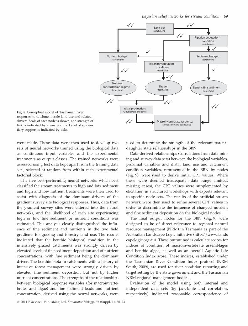
Fig. 8 Conceptual model of Tasmanian river

responses to catchment-scale land use and related

drivers. Scale of each node is shown, and strength of

link is indicated by arrow widths. Level of eviden-

tiary support is indicated by ticks.



observed and predicted condition, although declines in

%EPT under high-intensity forestry are greater at some

sites than the model predicts (e.g. Fig. 10). Further testing

is planned. In the future, this model can be used to

investigate the influence of varying combinations of

driver states on these aquatic biological indices. Diagnos-

tic application also is possible by fixing output node state

values and examining driver state probability distribu-

tions. Within set contexts (of dominant soil type, stream

reach slope, hydrological region, dominant land uses,

etc.), biological evidence can be entered into the BBN and

the probability of different states of selected drivers (such

as riparian condition, relative nutrient load, water use)

can be examined. The efficacy of a variety of different

management options in achieving specific target score

values or ranges can also be explored.

Discussion

An advantage of BBNs is their ability to exploit diverse

sources of information to explicitly represent probabilistic

relationships in a conceptually formulated causal chain.

The discipline of explicitly articulating a conceptual

model forces modellers and stakeholders to formally

evaluate and express beliefs concerning causal mecha-

nisms and facilitates model revision during development

(Burgman, 2005). The three cases illustrate alternative

approaches to the development of a BBN and the

flexibility this accords. With such a model, the effects of

different management options for stream systems can be

evaluated, and future conditions could be predicted based

on forecasts of land-use change or implementation of best

management practices. Running the model in the reverse

direction would facilitate diagnosis of the likely causes of

impairment to a stream given a set of biological charac-

teristics.

Fig. 10 Relationship between the percentage of benthic macroin

vertebrate taxa from the aquatic insect orders Ephemeroptera,

Plecoptera and Trichoptera (%EPT) and the proportion of area under

high-intensity forestry land use, for 26 Tasmanian catchments.

Values shown are from field survey (clear circles) and as outputs of

the Bayesian belief network (filled circles). Remaining land use in all

catchments is reservation and <10% low intensity forestry.

Fig. 9 Architecture of Tasmanian river Bayesian belief network showing input nodes on left, intermediate responses and site-scale benthic

responses in middle of graph, and output indicators on right. Measures of the invertebrate community condition include O ⁄ E (families

observed ⁄ expected), %EPT (per cent Ephemeroptera, Plecoptera and Trichoptera) and FFG (functional feeding groups). TRCI refers to the

Tasmanian River Condition Index.



The three case studies focus primarily on model

development; none was fully tested against independent

data. The elicitation model is broadly consistent with a

recent analysis of large data sets for clingers and

sediments (Pollard & Yuan, 2010), and the southeastern

Michigan case shows at least internal consistency. The

Tasmanian model has undergone preliminary testing

(Fig. 10) and initial results are encouraging. This model

will be extensively used in management decision-making

in the near future, which should provide further insight

into its utility.

The objective of the case study for characterising the

relationship between sedimentation and population den-

sity of macroinvertebrates was to demonstrate the feasi-

bility of using expert elicitation to build a BBN of a stream

ecosystem sub-model. To our knowledge, no empirical

data exist that would quantify the relationship depicted in

Fig. 4 for clingers, nor for the other functional groups

considered. Indeed, the mismatch we observed between

the variables that experts needed to express mechanistic

relationships (e.g. clinger density and per cent embedd-

edness) and the variables that were readily available from

field observations (e.g. clinger relative abundance and per

cent substratum sand ⁄fines) may be informative for

subsequent research towards defining mechanistic rela-

tionships in stream ecosystems. Furthermore, expert

judgment within a formalised modelling structure led to

a better understanding of causal relationships between

environmental stressors and population responses, and a

model outcome that participants believed was a reason-

able representation of the expected relationship. The

exercise of building such a model forced the team to

define the scope of the problem more precisely than

otherwise might be the case. Elicitation may be criticised

because of the difficulty of testing or evaluating the

models, but it can be the only reasonable option for model

development when appropriate data are difficult to

obtain, and it can provide useful insights into the most

pressing needs for future research and data collection.

Participants in the sedimentation elicitation case were in

agreement that the elicited model reflected their consen-

sus view of a stressor–response relationship considered to

be of wide significance in stream impairment.

The southeastern Michigan case developed directly

from field survey data was in essence an effort to explore

the ability of a limited number of prior variables to predict

stream condition, represented directly by habitat quality

and secondarily by species and functional diversity of the

fish assemblage. Both habitat quality and fish diversity

were predicted moderately well; however, the model was

not tested directly with an independent data set. Because

of its reliance on data from a specific region, it presumably

has the limited generality of a statistical analysis of the

same data; comparison with other data sets would be the

most reasonable test of the extent of its applicability

elsewhere. Attempts to use the Michigan model ‘in

reverse’, to infer causal conditions, were disappointing.

It seems likely that the relatively weak statistical associ-

ations used to develop the CPTs (e.g. Fig. 6) resulted in a

causal chain of low predictive strength, making it difficult

to work backwards from effect to probable cause. In their

model of eutrophication in the Neuse River estuary, North

Carolina, Borsuk et al. (2004) concluded that the further

down the causal chain a variable was, the greater the

predictive uncertainty.

The Tasmanian mixed model is the most detailed and

information-rich and likely holds the greatest promise for

rapid management utility and uptake. Two applications

have been developed from this BBN (see http://

www.landscapelogicproducts.org.au). Outcomes from

sets of scenarios have been documented in ‘fact sheets’

to inform managers in making investment decisions for

catchment and riparian management. These relate stream

health to a variety of combinations of land use, riparian

condition, and related ‘drivers’ in graphical and text form.

In addition, the BBN has been incorporated into a multi-

BBN decision support system for Tasmanian catchment

and natural resource managers to apply scenarios at

whole of catchment scales. Training has already been

conducted in its use in the three Tasmanian management

regions.

Presumably any of the models could be adapted to a

different setting, but probabilistic relationships likely are

specific to a rather narrow set of conditions, and the

variables and probabilistic relationships may need to be

re-considered as the problem setting diverges from the

original conception. Assuming that the goals are to depict

causal relationships and to help specific management

activities, each BBN is expected to be rather narrow in its

scope. The approach itself is flexible, however, as we have

attempted to illustrate with diverse examples.

Acknowledgments

The expert elicitation workshop was sponsored by the

Office of Research and Development, National Center for

Environmental Assessment, USEPA. Research on the

southeastern Michigan watersheds was supported by a

grant from the Water and Watersheds Program of EPA

and NSF. Tasmanian studies were supported by the

Landscape Logic Research Hub, with funding from the

Australian Commonwealth Environmental Research



Facilities scheme (Department of Environment, Water,

Heritage and the Arts). We thank W. Dodds, L. Johnson,

M. Palmer, B. Wallace and EPA staff for participation in

the expert elicitation process. We thank reviewers of the

manuscript and David Strayer for helpful comments.

References

Allan J.D. (2004) Landscape and riverscapes: the influence of

land use on river ecosystems. Annual Reviews of Ecology,

Evolution and Systematics, 35, 257–284.

Allan J.D. & Castillo M.M. (2007) Stream Ecology. Springer,

Dordrecht, The Netherlands.

ANDRL (2008) Australian Natural Resources Data Library.

Accessed online 24 March 2009 at: http://adl.brs.gov.au.

Barbour M.T., Gerritsen J., Snyder B.D. & Stribling J.B. (1999)

Rapid Bioassessment Protocols for Use in Streams and Wadeable

Rivers: Periphyton, Benthic Macroinvertebrates and Fish, 2nd

edn. EPA 841-B-99-002. U.S. Environmental Protection

Agency, Office of Water, Washington, D.C.

Borsuk M.E., Stow C.A. & Reckhow K.H. (2004) A Bayesian

network of eutrophication models for synthesis, predic-

tion, and uncertainty analysis. Ecological Modelling, 173,

219–239.

Bott T.L. (2006) Primary productivity and community respi-

ration. In: Methods in Stream Ecology (Eds F.H. Hauer &

G.A. Lamberti ), pp. 663–690. Academic Press, Burlington.

Burgman M.A. (2005) Risks and Decisions for Conservation and

Environmental Management. Cambridge University Press,

New York.

Davies P.E. (2000). Development of a national river bioas-

sessment system (AUSRIVAS) in Australia. In: Assessing the

Biological Quality of Freshwaters: RIVPACS and Other Tech-

niques. (Eds J.F. Wright , D.W. Sutcliffe & M.T. Furse ), pp.

113–124. Freshwater Biological Association, Cumbria, UK.

Davies P.E. & Nelson M. (1994) Relationships between

riparian buffer widths and the effects of logging on stream

habitat, invertebrate community composition and fish

abundance. Australian Journal of Marine and Freshwater

Research, 45, 1289–1305.

Davies P.E., Cook L.S.J., McIntosh P. & Munks S.A. (2005a)

Changes in stream biota along a gradient of logging

disturbance, 15 years after logging at Ben Nevis, Tasmania.

Forest Ecology and Management, 219, 132–148.

Davies P.E., McIntosh P., Wapstra M., Bunce S., Cook L.S.J.,

French B. et al. (2005b) Changes to headwater stream

morphology, habitats and riparian vegetation recorded

15 years after pre-Forest Practices Code forest clearfelling

in upland granite terrain, Tasmania, Australia. Forest

Ecology and Management 217, 331–350.

Davies P.E., Harris J.H., Hillman T.J. & Walker K.F. (2010)

The sustainable rivers audit: assessing river ecosystem

health in the Murray Darling Basin, Australia. Marine and

Freshwater Research, 61, 764–777.

Diana M.J., Allan J.D. & Infante D.M. (2006) The influence of

habitat and land use on fish assemblages of streams in

southeastern Michigan. In: Influences of Landscape on Stream

Habitats and Biological Assemblages (Eds R.M. Hughes, L.

Wang & P.W. Seelbach ), pp. 359–374. American Fisheries

Society, Symposium 48, Bethesda, MD.

Downes B.J. (2010) Back to the future: little-used tools and

principles of scientific inference can help disentangle

effects of multiple stressors on freshwater ecosystems.

Freshwater Biology 55(Suppl. 1), 60–79.

DPIW (2008) Conservation of Freshwater Ecosystem Values

(CFEV) Project Technical Report. Conservation of Freshwater

Ecosystem Values Program. Department of Primary Indus-

tries and Water, Hobart, Tasmania, 227 pp.

Farrand W.R. & Bell D.L. (1982) Quaternary Geology of

Southern Michigan (map). Department of Geological Sci-

ences, University of Michigan, Ann Arbor, MI.

Grace M.R. & Imberger S.J. (2006) Stream metabolism:

performing & interpreting measurements. Water Studies

Centre, Monash University, Murray Darling Basin

Commission and New South Wales Department of

Environment and Climate Change. 204 pp. Accessed online

1 April 2009 at: http://www.sci.monash.edu.au/wsc/

docs/tech-manual-v3.pdf.

Haas T.C., Mowrer H.T. & Shepperd W.D. (1994) Modeling

aspen stand growth with a temporal Bayes network.

Artificial Intelligence Applications, 8, 15–28.

Hershey A.E., Fortino K., Peterson B.J. & Ulseth A.J. (2006)

Stream food webs. In: Methods in Stream Ecology (Eds F.H.

Hauer & G.A. Lamberti ), pp. 637–661. Academic Press,

Burlington.

Hughes J.M.R. (1987) Hydrological characteristics and clas-

sification of Tasmanian rivers. Australian Geographical

Studies, 25, 61–82.

Hughes R.M., Wang L. & Seelbach P.W. (Eds) (2006)

Influences of Landscape on Stream Habitats and Biological

Assemblages. American Fisheries Society, Symposium 48,

Bethesda, Maryland.

Infante D.M. & Allan J.D. (2010) Response of stream fish

assemblages to local-scale habitat as influenced by land-

scape: a mechanistic investigation of stream fish assem-

blages. In: Community Ecology of Stream Fishes (Eds K.B.

Gido & D.A. Jackson ), pp. 371–400. American Fisheries

Society, Symposium 73, Bethesda, Maryland.

Infante D.M., Allan J.D., Linke S. & Norris R.H. (2008)

Relationship of fish and macroinvertebrate assemblages to

environmental factors: implications for community con-

cordance. Hydrobiologia, 623, 87–103.

Jensen F.V. (1996). An Introduction to Bayesian Networks. UCL

Press, London.

Jerie K., Houshold I. & Peters D. (2001) Stream diversity and

conservation in Tasmania: yet another new approach. In:

Proceedings of the 3rd Australian Stream Management Confer-

ence, CRC for Catchment Hydrology, Melbourne, Australia

pp. 329–335.



Jerie K., Houshold I. & Peters D. (2003) Tasmania’s River

Geomorphology: Stream Character and Regional Analysis, Vol.

1. Nature Conservation Report 03 ⁄5. Nature Conservation

Branch, DPIWE, Hobart, Tasmania, 66 pp.

Johnson L.B., Host G.E. (2010) Recent developments in

landscape approaches for the study of aquatic ecosystems.

Journal of the North American Benthological Society, 29,

41–66.

Korb K.B. & Nicholson A.E. (2004) Bayesian Artificial Intelli-

gence. Chapman and Hall ⁄CRC Press, London, 364 pp.

Kuikka S., Hilden M., Gislason H., Hansson S., Sparholt H. &

Varis O. (1999) Modeling environmentally driven uncer-

tainties in Baltic cod (Gadus morhua) management by

Bayesian influence diagrams. Canadian Journal of Fisheries

and Aquatic Sciences, 56, 629–641.

Lammert M. & Allan J.D. (1999) Assessing biotic integrity of

streams: effects of scale in measuring the influence of land

use ⁄ cover and habitat structure on fish and macroinverte-

brates. Environmental Management 23, 257–270.

Lee D.C. & Rieman B.E. (1997) Population viability

assessment of salmonids using probabilistic networks.

North American Journal of Fisheries Management, 17, 1144–

1157.

Michigan Department of Environmental Quality (MDEQ).

(1997) Qualitative biological and habitat survey protocols

for wadeable streams and rivers. MI ⁄DEQ ⁄SWQ-96 ⁄068.

NRM South (2009) Tasmanian River Condition Index Reference

Manual. NRM South, Hobart, Australia, 250 pp. Accessed

online 1 July 2009 at: http://www.nrmsouth.org.au/

uploaded/287/15130402_19trcireferencemanualweb.pdf

Paulsen S.G., Mayio A., Peck D.V., Stoddard J.L., Tarquino E.

& Holdsworth S.M. et al. (2008) Condition of stream

ecosystems in the US: an overview of the first national

assessment. Journal of the North American Benthological

Society, 27, 812–821.

Plowright R.K., Sokolow S.H., Gorman M.E., Daszak P. &

Foley J.E. (2008) Causal inference in disease ecology:

investigating ecological drivers of disease emergence.

Frontiers in Ecology and the Environment, 6, 420–429.

Pollard A.I. & Yuan L.L. (2010) Assessing the consistency of

response metrics of the invertebrate benthos: a comparison

of trait- and identify-based measures. Freshwater Biology 55,

1420–1429.

Pollino C.A., Woodberry O., Nicholson A., Korb K. & Hart

B.T. (2007) Parameterisation and evaluation of a Bayesian

network for use in an ecological risk assessment. Environ-

mental Modelling and Software 22, 1140–1152.

Pringle C.M. & Triska F.J. (2006) Effects of nutrient enrich-

ment on periphyton. In: Methods in Stream Ecology (Eds F.H.

Hauer & G.A. Lamberti ), pp. 743–760. Academic Press,

Burlington.

Rieman B.E., Peterson J.T., Clayton J., Howell P., Thurow R.,

Thompson W. et al. (2001) Evaluation of potential effects of

federal land management alternatives on trends of salmo-

nids and their habitats in the interior Columbia River

basin. Forest Ecology and Management, 153, 43–62.

Roth N.E., Allan J.D. & Erickson D.L. (1996) Landscape

influences on stream biotic integrity assessed at multiple

spatial scales. Landscape Ecology, 11, 141–156.

Smith B.J., Davies P.E. & Munks S.A. (2009) Changes in

benthic macroinvertebrate communities in upper catch-

ment streams in Tasmania across a gradient of catchment

forest operation history. Forest Ecology and Management,

257, 2166–2174.

Steel E.A., Hughes R.M., Fullerton A.H. et al. (2010) Are we

meeting the challenges of landscape-scale riverine re-

search? A review. Living Reviews in Landscape Research

4, 1. Available at: http://www.livingreviews.org/lrlr-

2010-1 (accessed on 14 July 2010).

Stewart-Koster B., Bunn S.E., Mackay S.J., Poff N.L.,

Naiman R.J. & Lake P.S. (2005) The use of Bayesian

networks to guide investments in flow and catchment

restoration for impaired river ecosystems. Freshwater

Biology, 55, 243–260.

Townsend C.R., Downes B.J., Peacock K. & Arbuckle C.J.

(2004) Scale and the detection of land-use effects on

morphology, vegetation and macroinvertebrate communi-

ties of grassland streams. Freshwater Biology, 49, 448–462.

US Environmental Protection Agency (EPA) (2000) The

Quality of our Nation’s Waters: a Summary of the National

Water Quality Inventory 1998 Report to Congress. EPA 841-S-

00-001. Office of Water, Washington, DC.

Webb J.A., Stewardson M.J. & Koster W.M. (2010) Detecting

ecological responses to flow variation using Bayesian

hierarchical models. Freshwater Biology, 55, 108–126.

Yuan L.L. (2004) Assigning macroinvertebrate tolerance

classifications using generalized additive models. Freshwa-

ter Biology, 49, 662–677.

(Manuscript accepted 1 August 2011)



investigating the relationships between environmental stressors

Documents