investigation and optimization of a dry bulk terminal
TRANSCRIPT

Treball de Fi de Màster
Master in Supply Chain, Transport and Mobility
Investigation and optimization of a dry bulk terminal
capacity using queuing theory. Application at the
cement terminal in Barcelona Port.
Author: Meritxell Boixadé Cuadrat
Director: Manel Grifoll Colls
Call: September 2018
Escola Tècnica Superior d’Enginyeria Industrial de Barcelona

Investigation and optimization of a dry bulk terminal capacity using queuing theory
1
ABSTRACT
This report presents the analysis of the performance of Portcemen Terminal in Port of Barcelona.
From the actual data of bulk carriers calls throughout the year 2015 collected and provided by
such terminal, a statistical analysis of its patterns have been developed. At the same time, it is
intended to provide an overview of solid bulk maritime transport and its operations.
In order to characterize and analyse the fulfilment of Portcemen Terminal, Queuing Theory has
been applied as a function of different parameters such as the average waiting time of the vessels
in the queue or the occupation factor of the berthing line, among other. As a first step of a terminal
optimization process, service levels of the terminal have been investigated according the standard
design parameters established by the Spanish Recommendations of Maritime Works (ROM) and
UNCTAD. Finally, to carry out the resilience study of the cement terminal through performance
indicators, various scenarios have been raised.
The main conclusions derived from this report are the following. Firstly, with the calculations of
the parameters for the selected queuing model for the demand in 2015, it can be asserted that it is
an over dimensioned system. With a demand of 58 vessels per year in 2015, the probability of the
system being empty is extremely high (83%) and the probability of having one vessel in the
system is only 14%. This fact reflects that most time of the year the terminal is empty.
Nevertheless, it has to be borne in mind that the traffic in 2015 was only the 60% approximately
of the traffic before the financial crisis of 2008 in Spain that represented one of the most
significant setback in global trade. Yet, maritime shipping is subject to fluctuations as commercial
opportunities change. This is an added difficulty of predicting traffic to dimensioning maritime
terminals. Although Portcemen terminal is not one of the biggest cement terminals in the world,
for sure it has had and it will have greater volume of dry bulk traffic than it has now.
Moreover, port selection is especially relevant because of the strong link between ports and
industrial activity, but particularly between the port and its hinterland. Bulk terminals are better
discussed in terms of concentration. They are found in regions heavily involved in the bulk trades.
These bulk ports, are not only engaged in linking sea and land transport but are also hubs of
industrial activity. The maritime traffic associated with transport of semi-raw materials and
intermediate products activities is thus highly consistent and varies according to cyclic demand
patterns.

Investigation and optimization of a dry bulk terminal capacity using queuing theory
2
Table of contents
ABSTRACT .................................................................................................................................. 1
LIST OF FIGURES ....................................................................................................................... 4
LIST OF ABBREVIATIONS ....................................................................................................... 7
1. INTRODUCTION ................................................................................................................. 8
1.1. Objectives .................................................................................................................... 10
1.2. Stages of the research .................................................................................................. 10
1.3. Structure and summary of the contents ....................................................................... 10
1.4. Justification of the thesis ............................................................................................. 11
2. STATE-OF-ART ................................................................................................................. 15
2.1. Port of Barcelona ......................................................................................................... 15
2.2. Portcemen, S.A. ........................................................................................................... 16
2.3. Cement and clinker trade ............................................................................................. 19
2.3.1. Cement and clinker evolution.............................................................................. 19
2.3.2. Global trade and distribution flows ..................................................................... 21
2.4. Overview of cement and clinker in maritime transport ............................................... 23
2.4.1. Forms of transportation ....................................................................................... 23
2.4.2. Bulk ships ............................................................................................................ 24
2.4.3. Size categories ..................................................................................................... 26
2.4.4. Port facilities ....................................................................................................... 27
2.4.5. Bulk cement terminals and coastal grinding plants ............................................. 27
2.4.6. Cement terminals ................................................................................................. 28
2.4.7. Required infrastructure in cement terminals ....................................................... 28
2.4.8. Loading and unloading process ........................................................................... 29
2.4.9. Cement and clinker properties ............................................................................. 34
2.5. Description of the data ................................................................................................ 35
3. METHODS ......................................................................................................................... 36
3.1. Queuing theory ............................................................................................................ 36
3.1.1. Fundamentals ...................................................................................................... 37
3.1.2. Main parameters. Notation of queuing theory ..................................................... 43
3.1.3. Modelling ship arrival process ............................................................................ 44
3.1.4. Modelling inter-arrival time ................................................................................ 45
3.1.5. Modelling service time ........................................................................................ 46
3.1.6. Research methodology ........................................................................................ 46
3.2. M/M/1 ......................................................................................................................... 48
4. RESULTS ........................................................................................................................... 50
Investigation and optimization of a dry bulk terminal capacity using queuing theory
3
4.1. Current situation .......................................................................................................... 50
4.1.1. Sources of the data .............................................................................................. 50
4.1.2. General information ............................................................................................ 51
4.1.3. Assumptions ........................................................................................................ 59
4.1.4. Inputs and outputs of the model .......................................................................... 59
4.1.5. Calculations of the parameters for the selected queuing model .......................... 60
4.1.6. Simulation ........................................................................................................... 65
4.1.7. Levels of service .................................................................................................. 69
4.2. Future situation ............................................................................................................ 72
5. DISCUSSION AND CONCLUSIONS ............................................................................... 77
BIBLIOGRAPHY ....................................................................................................................... 81
ANNEX ....................................................................................................................................... 83
Investigation and optimization of a dry bulk terminal capacity using queuing theory
4
LIST OF FIGURES
Figure 1. International Seaborne Trade and Exports of Goods Evolution, 1955-2016. Source:
World Bank. United Nations, Review of Maritime Transport. Figure 2. Growth in international seaborne trade between 1970-2016 (in millions of tons
loaded). Elaborated by the author. Source: Compiled by the UNCTAD secretariat. Figure 3. Baltic Dry Index (2015-2018). Between these years, the highest value in the last years
and the historic low have been achieved. Source: www.investing.com Figure 4. Annual evolution of cement export volumes (in thousands tons) of Spain between
2005 and 2015. Source: https://es.statista.com Figure 5. Evolution of foreign trade in the Spanish cement sector (in thousands tons) separated
by type of cargo (cement and clinker) and type of activity (import and export). Source: Anuario
del sector cementero español 2016. https://www.oficemen.com Figure 6. Evolution of solid bulk volumes of Port of Barcelona between 2005-2017 in tons.
Source: Elaborated by the author. Data compiled from Puertos del Estado.
Figure 7. Evolution of solid bulk volumes of all Spanish port authorities between 2005-2017 in
tons. Source: Elaborated by the author. Data compiled from Puertos del Estado. Figure 8. Aerial photo of Port of Barcelona. Source: Barcelona Port Authority. Figure 9. Localization of Portcemen terminal in Port of Barcelona. It is situated in Contradic
Sud Wharf next to Ergransa and Bunge Ibérica (both dedicated to solid bulks). Source:
Barcelona Port Authority. Figure 10. Aerial view of Portcemen Terminal. Source: Google Maps. Figure 11. Floor plant of Portcemen facilities. It shows the arrangement of the 12 silos located
in a battery of 6 silos parallel to the dock. It also shows the loading and unloading equipment
and the conveyor belt. Source: http://www.portcemen.com Figure 12. Portcemen terminal in Port of Barcelona. It can be seen the 12 silos, the conveyor
belt and the loading and unloading equipment of the terminal. Source: Google Maps Figure 13. Global seaborne cement and clinker trade flows in 2015. As can be seen in Spain,
since 2008, clinker production is bigger than its consumption when years ago, the situation was
the opposite. Source: https://cementdistribution.com Figure 14. Clinker and cement trade by water in 2015 in million tons. It is distinguished
between seaborne trade (international and domestic) and inland water domestic trade by type of
product. Source: https://cementdistribution.com Figure 15. Clinker and cement trade by vessel type in 2015 in million tons. It is distinguished
between bulk carriers, self-discharging cement carriers and inland ships and water barges.
Source: https://cementdistribution.com Figure 16. Ship’s length versus the ship’s deadweight. Source: Elaborated by the author based
on the databases of the Sea-web and Marinetraffic. Figure 17. Ship’s beam and ship’s maximum draft versus the ship’s deadweight. Source:
Elaborated by the author based on the databases of the Sea-web and Marinetraffic. Figure 18. Classification by type and main characteristics of bulk ships. Source: Elaborated by
the author through own research in vessels data basis. Figure 19. Number of vessels served in Portcemen terminal in 2015 by type of vessels. Source:
Elaborated by the author. Figure 20. Overview of facilities of the top five multinationals involved in waterborne trade and
distribution in 2013. Cemex (the fourth in the world) is one of the three cement companies that
owns Portcemen terminal. Source: www.cemnet.com. Figure 21. Example of travelling ship-loader with material from high-level conveyor. Source:
Chapter II: Planning Principles. Port Development: A Handbook for Planners in Developing
Countries (UNCTAD)

Investigation and optimization of a dry bulk terminal capacity using queuing theory
5
Figure 22. Functional diagram of cement or clinker loading operations in Portcemen terminal.
Source: Duran E., Portcemen terminal Figure 23. Revolving grabbing crane diagram. Source: Chapter II: Planning Principles. Port
Development: A Handbook for Planners in Developing Countries (UNCTAD) Figure 24. Pneumatic system in an unloading operation suctioning cement from a bulk carrier.
Source: https://www.conveyorspneumatic.com Figure 25. Portable pneumatic handling equipment. A: Combination vacuum/pressure system;
conveying grain from ship into bagging hopper. B: Combination vacuum/pressure system;
conveying grain from ship to barge. Source: Chapter II: Planning Principles. Port Development:
A Handbook for Planners in Developing Countries (UNCTAD)
Figure 26. Clinker in bulk. Source: http://www.wigginsbuildingsupplies.co.uk
Figure 27. Cement in bulk. Source: http://www.cargohandbook.com
Figure 28. Queuing System Diagram. Source: Elaborated by the author. Figure 29. Ship queue at the seaport diagram. Source: Elaborated by the author. Figure 30. Overview of proposed inter-arrival time distributions (IATDist). For dry bulk cargo,
it proposes Weibull, Erlang-2 and negative exponential (NED) distributions. Source: Van
Vianen, T., Simulation-Integrated Design of Dry Bulk Terminals Figure 31. Overview of proposed service time distributions (WsDist). For dry bulk cargo, it
proposes Normal, Gamma and Erlang-k distributions. Source: Van Vianen, T., Simulation-
Integrated Design of Dry Bulk Terminals Figure 32. Multiple server M/M/c diagram. Figure 33. Single server M/M/1 diagram. Figure 34. Graphical illustration and verification of Little's Result. N is the average number of
customers in the system shown in the graphic as the gap between arrivals and departures.
Source: Sanjay K. Bose Figure 35. Description of the main parameters applied in queuing theory formulas. Apart from
their notation, it is also shown their unit of measure. Source: Elaborated by the author.
Figure 36. Representation of the relationships between the main parameters of queuing theory
based on the waiting area and the service node. Source: University of Pittsburg. Figure 37. Diagram of M/M/1/infinite/FIFO queue. It shows the queue and the server along with
the arrival rate and service rate. Source: Elaborated by the author. Figure 38. Calls per month in Portcemen terminal in 2015. Source: Elaborated by the author Figure 39. Cement and clinker volumes in Portcemen terminal in 2015. As can be noted, clinker
volumes are much higher than cement volumes. Moreover, it can be seen the significant
fluctuation of the volumes. Source: Elaborated by the author Figure 40. Cement and clinker month evolution in Portcemen terminal in tons. Source:
Portcemen Terminal Figure 41. Inter-arrival histogram with the frequency polygon. Source: Elaborated by the author Figure 42. Parameters of inter-arrival histogram. Source: Elaborated by the author Figure 43. Inter-arrival histogram with the cumulative frequency. Source: Elaborated by the
author Figure 44. Parameters of Kolmogorov-Smirnov test to determine the goodness of fit to the
exponential distribution. Source: Elaborated by the author Figure 45. Table of Kolmogorov-Smirnov test estimator of Goodness of Fit. Marked in red, the
calculation of 𝐷 ∝ for an n>50 and α=0.05. Source:
http://www4.ujaen.es/~mpfrias/TablasInferencia.pdf Figure 46. Arrivals in Portcemen terminal in 2015. Source: Elaborated by the author Figure 47. Ships arrival distribution as Poisson function, hypothetical port. Source: El-Naggar,
M. E., Application of queuing theory to the container terminal at Alexandria seaport. Figure 48. Number of arrivals per month in Portcemen Terminal in 2015. Source: Elaborated by
the author.

Investigation and optimization of a dry bulk terminal capacity using queuing theory
6
Figure 49. Parameters of Kolmogorov-Smirnov test to determine the goodness of fit to the
Poisson distribution. Source: Elaborated by the author Figure 50. Inputs and outputs in a queuing system. Source: Elaborated by the author Figure 51. Summary of the values of the parameters calculated for the selected queuing model
M/M/1. Source: Elaborated by the author. Figure 52. Summary table of the values of all probabilities calculated. Source: Elaborated by the
author.
Figure 53. Summary of the values of the parameters calculated for the selected queuing model
M/M/1 versus M/D/1 model. Source: Elaborated by the author. Figure 54. Simulation analysis. Source: Elaborated by the author. Figure 55. Summary of the values calculated. Source: Elaborated by the author. Figure 56. Values of the parameters by increasing the demand. Source: Elaborated by the author Figure 57. Performance of the terminal if the demand increases. Source: Elaborated by the
author Figure 58. Values of the parameters by increasing the servers and the demand. Source:
Elaborated by the author Figure 59. Performance of the terminal if the servers increase. Source: Elaborated by the author Figure 60. Summary of the performance of the terminal if the demand increases. Source:
Elaborated by the author Figure 61. Summary of the performance of the terminal if the servers increase. Source:
Elaborated by the author

Investigation and optimization of a dry bulk terminal capacity using queuing theory
7
LIST OF ABBREVIATIONS
APB Barcelona Port Authority
BDI Baltic Dry Index
CTMC Continuous time Markov chain
dwt Deadweight tonnage
FIFO First In First Out
FO Observed frequency
FOR Relative observed frequency
FORA Accumulated relative observed frequency
FERA Accumulated relative expected frequency
IAT Inter-arrival times
JIT Just in time
LIFO Last In, First Out
m Meters
MT Million tons
NED Negative Exponential Distribution
PR Priority
ROM Recommendations of Maritime Works
RS Random Service
t Tons
Tm Metric tons
UNCTAD United Nations Conference on Trade and Development
Investigation and optimization of a dry bulk terminal capacity using queuing theory
8
1. INTRODUCTION
Shipping has been an important human activity throughout history, particularly where prosperity
depended primarily on international and interregional trade. In fact, transportation has been called
one of the four cornerstones of globalization, along with communications, international
standardization, and trade liberalization [Kumar and Hoffmann, 2002]. Due to a number of
technological, economic, and socio-cultural forces, seldom country can keep itself fully isolated
from the economic activities of other countries. Indeed, many countries have seen impressive
economic growth in the recent past due to their willingness to open their borders and markets to
foreign investment and trade. This increased flow of knowledge, resources, goods, and services
among our world’s nations is called “globalization”, formally defined as “the development of an
increasingly integrated global economy marked especially by free trade, free flow of capital, and
the tapping of cheaper foreign labor markets.” (Merriam-Webster, www.merriam-
webster.com/dictionary/globalization, accessed 2018).
The marine industry is an essential link in international trade, with ocean-going vessels
representing the most efficient, and often the only method of transporting large volumes of basic
commodities and finished products [Gardiner, 1992].
Maritime transport remains the dominant mode for international trade both for bulk transport of
commodities and containerized break-bulk cargo. The economics of bulk transport still influence
the trade patterns and industrial location. Intermodal transport has become a global phenomenon
as mechanized handling and containerization have reduced handling costs between modes and
promoted their efficiency. Ports have become elements in global commodity chains controlled by
logistics companies, maritime shipping lines, freight forwarders and transport operators. Their
strategies and the allocation of their assets have shaped the structure of maritime transport
networks in terms of ports of call, hierarchy and frequency of services [Rodrigue J.P. and Browne
M., 2014].
The development of bulk and containerized maritime transportation has been strongly influenced
by technology [Pinder and Slack, 2004]. Port selection is especially relevant because of the strong
link between ports and industrial activity, but particularly between the port and its hinterland.
However, technology and vessel design are by no means the only factors at work to influence the
patterns of the world maritime shipping; government policy, commercial buying practices and
physical constraints such as water depth in ports also play a key role. Bulk terminals are better
discussed in terms of concentration. They are found in regions heavily involved in the bulk trades.
These bulk ports, are not only engaged in linking sea and land transport but are also hubs of
industrial activity. In the bulk trades, as in maritime transport in general, there is now a realization
that the integration of supply chains requires a high level of organizational interdependence.
Maritime transportation and inland transportation must increasingly be seen as functionally
integrated. In bulk the reduction of inventory and storage costs by just-in-time (JIT) shipments
and door-to-door services are increasing in significance.
Geographically, bulk cargo shows a remarkable stability, particularly in terms of its origins. The
extraction and shipment of natural resources, such as minerals and oil, is bound to the geological
setting, require massive capital investments and takes place over decades. Globalization identified
labor markets overseas that encouraged transport of semi-raw materials and intermediate products
where manufacturing costs were lower. The maritime traffic associated with these activities is
thus highly consistent and varies according to cyclic demand patterns.

Investigation and optimization of a dry bulk terminal capacity using queuing theory
9
Marine transportation is an integral, if sometimes less publicly visible, part of the global economy.
The growth of maritime transportation is strongly correlated with the growth of international trade
as maritime shipping and ports are the main physical support for international trade flows. From
about 800 million tons of loaded cargo in 1955, maritime traffic exceeded 8 billion tons for the
first time in 2007, which represents 32,500 ton-miles. Yet, maritime shipping is subject to
fluctuations as commercial opportunities change. The financial crisis of 2008-2009 represented
the most significant setback in global trade since the Great Depression in the 1930s, but global
trade and maritime shipping recovered afterwards.
Figure 1. International Seaborne Trade and Exports of Goods Evolution, 1955-2016. Source: World Bank. United
Nations, Review of Maritime Transport.
Investigation and optimization of a dry bulk terminal capacity using queuing theory
10
1.1.Objectives
The present minor thesis examines the performance of the Portcemen Terminal in Port of
Barcelona. The main objective is to characterize and analyze the fulfilment of Portcemen terminal
in Barcelona Port applying the queuing theory in order to investigate the service levels using
standard design parameters (Spanish Recommendations of Maritime Works1 or UNCTAD2) as a
first step of a terminal optimization process. The sub-goal of the thesis is to carry out a resilience
study of the cement terminal in Barcelona Port through performance indicators.
1.2.Stages of the research
So that the objectives above-mentioned can be achieved, the following work phases have been
followed:
- First of all, some bibliographic review studies about cement and clinker trade, dry bulk
terminals and queuing theory have been research.
- A main objective and other sub-goals have been defined considering all relevant factors.
- Description of the case study and data processing.
- Application of the methodology applied at the cement terminal in Barcelona Port.
- Contrasting and analysis of results.
- Discussion and conclusions.
1.3.Structure and summary of the contents
This document is organised as follows:
In chapter 2 is presented the State-of-art. First, a brief resume of the international cement
and clinker trade and the general distribution flows, as well as the description of
specialized bulk ships and cement terminals with their required infrastructure. It is also
described the loading and unloading process of cement and clinker and the required
equipment to carry it out. Moreover, a brief overview of Barcelona Port and Portcemen
terminal is provided to put the lector in situation about the characteristics of the terminal
analysed.
Chapter 3 presents the methodologies which have been used to carry out this minor thesis.
The queuing theory and different models are presented in order to be applied in the
Portcemen Terminal. Additionally, ship arrival process, inter-arrival time and service
time are modelled in order to be expressed in terms of probability distributions. The
Kolmogorov-Smirnov test it is used to determine the goodness of fit to such distributions.
1 R.O.M., Recommendations of Maritime Works, is a Programme of recommendations materialized by
Puertos del Estado that started in 1987 by order of the Directorate General for Ports and Coasts of the
Ministry of Public Works and Urban Development. 2 UNCTAD, United Nations Conference on Trade and Development, is a permanent intergovernmental
body established by the United Nations General Assembly in 1964.
Investigation and optimization of a dry bulk terminal capacity using queuing theory
11
In chapter 4 are presented the results obtained through the application of previous
mentioned methods so as to investigate the levels of service of the terminal using standard
design parameters (ROM and UNCTAD) as a first step of a terminal optimization process
and its general performance. Besides, a manual simulation with the data provided has
been carried out.
Chapter 5 presents the discussion and conclusions of the results.
1.4.Justification of the thesis
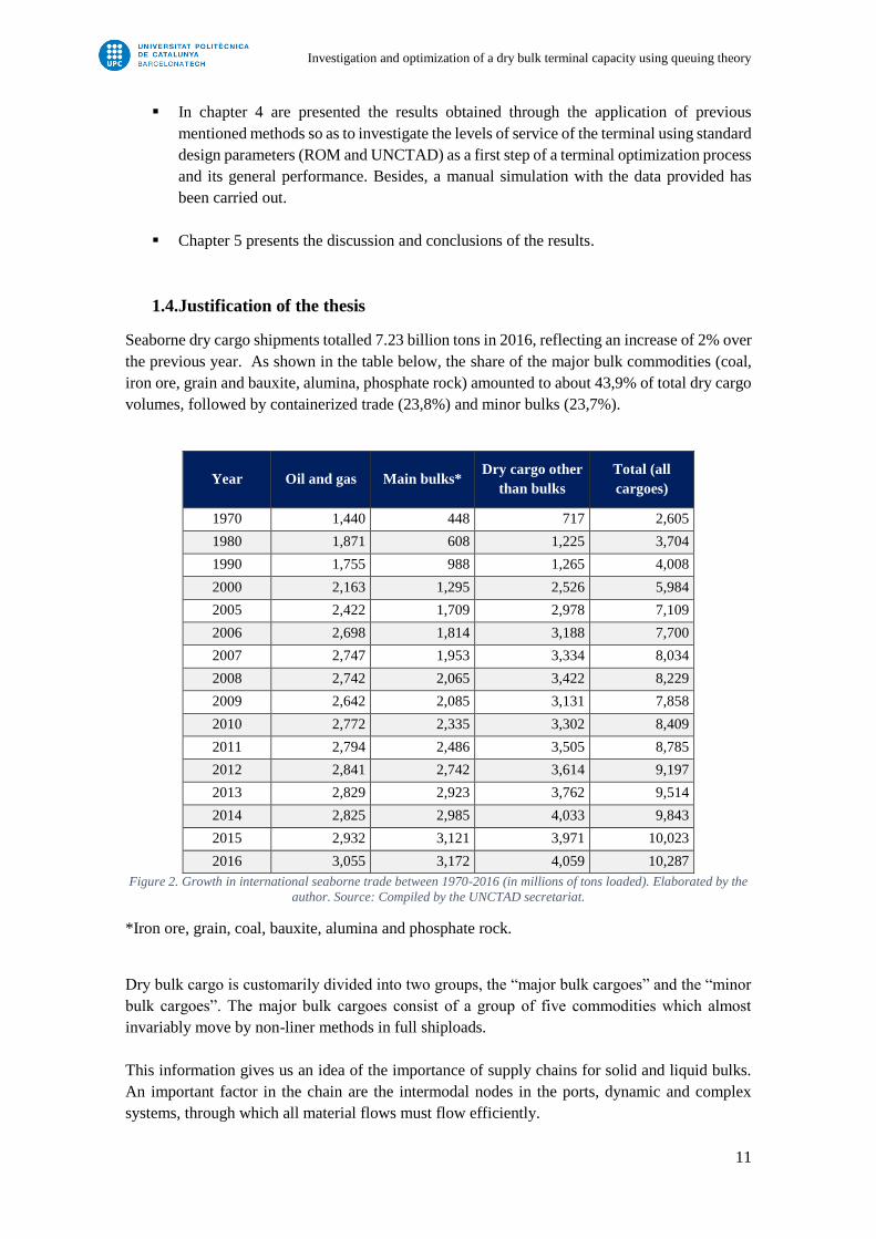
Seaborne dry cargo shipments totalled 7.23 billion tons in 2016, reflecting an increase of 2% over
the previous year. As shown in the table below, the share of the major bulk commodities (coal,
iron ore, grain and bauxite, alumina, phosphate rock) amounted to about 43,9% of total dry cargo
volumes, followed by containerized trade (23,8%) and minor bulks (23,7%).
Year Oil and gas Main bulks* Dry cargo other
than bulks
Total (all
cargoes)
1970 1,440 448 717 2,605
1980 1,871 608 1,225 3,704
1990 1,755 988 1,265 4,008
2000 2,163 1,295 2,526 5,984
2005 2,422 1,709 2,978 7,109
2006 2,698 1,814 3,188 7,700
2007 2,747 1,953 3,334 8,034
2008 2,742 2,065 3,422 8,229
2009 2,642 2,085 3,131 7,858
2010 2,772 2,335 3,302 8,409
2011 2,794 2,486 3,505 8,785
2012 2,841 2,742 3,614 9,197
2013 2,829 2,923 3,762 9,514
2014 2,825 2,985 4,033 9,843
2015 2,932 3,121 3,971 10,023
2016 3,055 3,172 4,059 10,287
Figure 2. Growth in international seaborne trade between 1970-2016 (in millions of tons loaded). Elaborated by the
author. Source: Compiled by the UNCTAD secretariat.
*Iron ore, grain, coal, bauxite, alumina and phosphate rock.
Dry bulk cargo is customarily divided into two groups, the “major bulk cargoes” and the “minor
bulk cargoes”. The major bulk cargoes consist of a group of five commodities which almost
invariably move by non-liner methods in full shiploads.
This information gives us an idea of the importance of supply chains for solid and liquid bulks.
An important factor in the chain are the intermodal nodes in the ports, dynamic and complex
systems, through which all material flows must flow efficiently.
Investigation and optimization of a dry bulk terminal capacity using queuing theory
12
The problems of handling bulk solids (storage, transport and process) are frequently the main
causes of problems in bulk flow management. A bad design of the node of nodal exchange, can
generate that the flow run into bottlenecks which generate delays and unnecessary costs. So
looking for the maximum efficiency and productivity of the installation is key in the flow of the
chain in the operation of bulk, bearing in mind those environmental problems derived from the
activity.
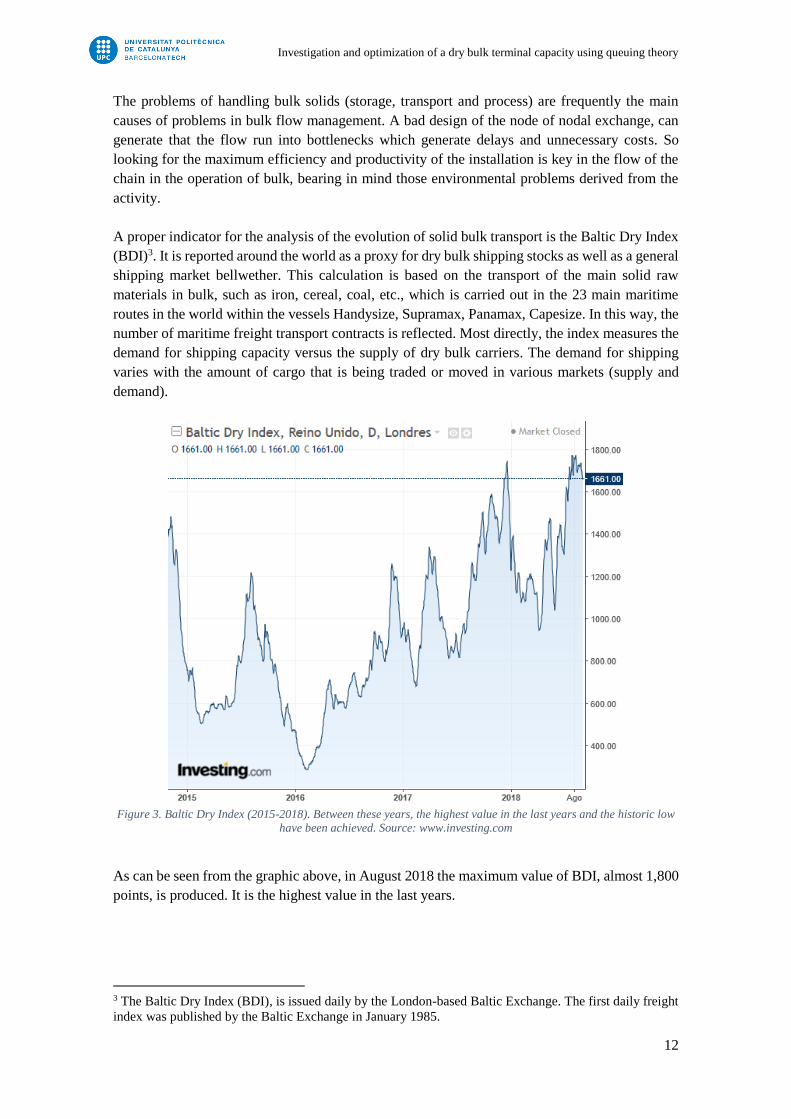
A proper indicator for the analysis of the evolution of solid bulk transport is the Baltic Dry Index
(BDI)3. It is reported around the world as a proxy for dry bulk shipping stocks as well as a general
shipping market bellwether. This calculation is based on the transport of the main solid raw
materials in bulk, such as iron, cereal, coal, etc., which is carried out in the 23 main maritime
routes in the world within the vessels Handysize, Supramax, Panamax, Capesize. In this way, the
number of maritime freight transport contracts is reflected. Most directly, the index measures the
demand for shipping capacity versus the supply of dry bulk carriers. The demand for shipping
varies with the amount of cargo that is being traded or moved in various markets (supply and
demand).
Figure 3. Baltic Dry Index (2015-2018). Between these years, the highest value in the last years and the historic low
have been achieved. Source: www.investing.com
As can be seen from the graphic above, in August 2018 the maximum value of BDI, almost 1,800
points, is produced. It is the highest value in the last years.
3 The Baltic Dry Index (BDI), is issued daily by the London-based Baltic Exchange. The first daily freight
index was published by the Baltic Exchange in January 1985.

Investigation and optimization of a dry bulk terminal capacity using queuing theory
13
When the world economy is in crisis, contracts for the transport of raw materials are reduced and
consequently the Baltic Dry Index falls. Therefore, it is considered an advanced indicator of the
market and is revealed as an effective thermometer of the evolution of the world economy.
As can be seen in the graphic above, this index of maritime freight of dry bulk cargo, on February
2016 reached the historic low of 290 points. By November 2016, it rebounded to over 1,000
sending the entire shipping industry to massive gains.
Cement is as vital a commodity to fast-growing economies as oil or steel. No other material is as
versatile when it comes to building houses, roads and big chunks of infrastructure. It is a huge
business: the world’s cement-makers rake in revenues of $250 billion a year. Outside China,
which accounts for half of global demand and production, six vast international firms—Buzzi,
Cemex, Heidelberg, Holcim, Italcementi and Lafarge—together have 40% or so of the market.
Cement consumption in Spain closed 2017 with a growth of 11%, which places the domestic
demand last year around 12.3 million tons. This confirms, therefore, the beginning of the recovery
of the sector, although this percentage, in absolute values, only means a growth of just over one
million tons, a reduced figure if we take into account that since 2007 the cement industry has lost
80% of its activity volume.
The consumption of cement in civil works has been reduced by 75% in the last decade, going
from 19Mt in 2008 to 5Mt in 2017. This situation confirms that the construction activity remains
stagnant at levels much lower than the normal volume of activity for a country like Spain, which
according to the average of the last 40 years and excluding the decade of the boom, should be
around 25 million tons annual.
Figure 4. Annual evolution of cement export volumes (in thousands tons) of Spain between 2005 and 2015. Source:
https://es.statista.com

Investigation and optimization of a dry bulk terminal capacity using queuing theory
14
Figure 5. Evolution of foreign trade in the Spanish cement sector (in thousands tons) separated by type of cargo
(cement and clinker) and type of activity (import and export). Source: Anuario del sector cementero español 2016.
https://www.oficemen.com
The export volume closed the year 2017 below 4 million tons, exactly in 3,762,911 tons with a
drop motivated by the loss of competitiveness of the sector due mainly to the increase in electricity
costs. The Spanish industry currently sustain one of the highest costs in Europe - up to 30% more
expensive - which penalizes its external competitiveness. This circumstance, which is reducing
the margin gained with the improvement of the domestic market, has stagnated the production
volumes of Spanish cement factories by 50% of its installed capacity, a level very similar to that
reached in the last five years, in those that the internal consumption was smaller.
As can be seen in the figure 4, the graphic shows the evolution of cement and clinker both export
and import separately. It can be noted a turning point in year 2008 due to the financial crisis that
Spain suffered. The main cause of Spain's crisis was the housing bubble and the accompanying
unsustainably high GDP growth rate. The ballooning tax revenues from the booming property
investment and construction sectors kept the Spanish government's revenue in surplus, despite
strong increases in expenditure, until 2007.
This fact is reflected in the graphic above, where until 2007 there was a substantial urbanization
growth and consequently, a significant need of cement which have to be imported due to the lack
of enough production in Spain. At this time, the consumption of this material was significantly
higher than its production. For this reason, the most part of the cement and clinker was imported
to Spain whereas exportations were nearly zero. From that moment, things were turned around
by diminishing the importations to zero in 2017 and increasing the exportations for both cement
and clinker. As can be noticed, cement trade is significantly variable and uncertain. For that
reason, resilience studies based on this trade have particular importance for the lack of
predictability of it.
Investigation and optimization of a dry bulk terminal capacity using queuing theory
15
2. STATE-OF-ART
2.1.Port of Barcelona
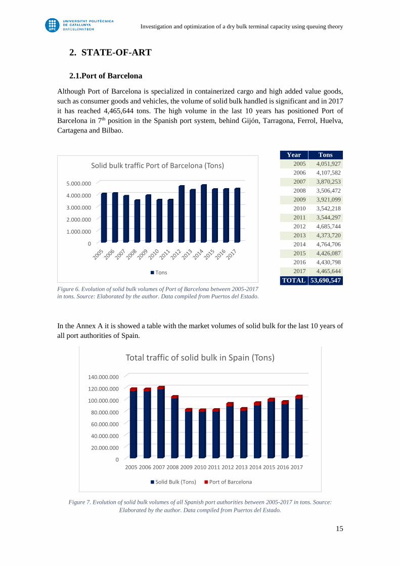
Although Port of Barcelona is specialized in containerized cargo and high added value goods,
such as consumer goods and vehicles, the volume of solid bulk handled is significant and in 2017
it has reached 4,465,644 tons. The high volume in the last 10 years has positioned Port of
Barcelona in 7th position in the Spanish port system, behind Gijón, Tarragona, Ferrol, Huelva,
Cartagena and Bilbao.
In the Annex A it is showed a table with the market volumes of solid bulk for the last 10 years of
all port authorities of Spain.
Figure 7. Evolution of solid bulk volumes of all Spanish port authorities between 2005-2017 in tons. Source:
Elaborated by the author. Data compiled from Puertos del Estado.
0
20.000.000
40.000.000
60.000.000
80.000.000
100.000.000
120.000.000
140.000.000
2005 2006 2007 2008 2009 2010 2011 2012 2013 2014 2015 2016 2017
Total traffic of solid bulk in Spain (Tons)
Solid Bulk (Tons) Port of Barcelona
Year Tons
2005 4,051,927
2006 4,107,582
2007 3,870,253
2008 3,506,472
2009 3,921,099
2010 3,542,218
2011 3,544,297
2012 4,685,744
2013 4,373,720
2014 4,764,706
2015 4,426,087
2016 4,430,798
2017 4,465,644
TOTAL 53,690,547
0
1.000.000
2.000.000
3.000.000
4.000.000
5.000.000
Solid bulk traffic Port of Barcelona (Tons)
Tons
Figure 1. Evolution of solid bulk volumes of Port of Barcelona 2005-2017 in tons. Source: Puertos del Estado. Figure 6. Evolution of solid bulk volumes of Port of Barcelona between 2005-2017
in tons. Source: Elaborated by the author. Data compiled from Puertos del Estado.
Investigation and optimization of a dry bulk terminal capacity using queuing theory
16
With 4.5 million tons, this year (2017) almost the same solid bulk volume was channeled through
the Port as compared to the previous year (+0,8%).
Although some products with huge volume have remained stable or have grown very lightly, such
as cement and clinker and cereals and flour, the increase in feed and fodder stands out by 50.3%
compared to 2015. In part, soy bean and potash have had decreases of 18.1% and 10.9%
respectively, mainly driven by eventual market and operating circumstances.
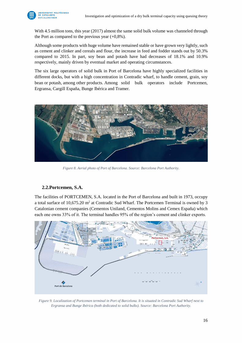
The six large operators of solid bulk in Port of Barcelona have highly specialized facilities in
different docks, but with a high concentration in Contradic wharf, to handle cement, grain, soy
bean or potash, among other products. Among solid bulk operators include Portcemen,
Ergransa, Cargill España, Bunge Ibérica and Tramer.
Figure 8. Aerial photo of Port of Barcelona. Source: Barcelona Port Authority.
2.2.Portcemen, S.A.
The facilities of PORTCEMEN, S.A. located in the Port of Barcelona and built in 1973, occupy
a total surface of 10,675.20 m2 at Contradic Sud Wharf. The Portcemen Terminal is owned by 3
Catalonian cement companies (Cementos Uniland, Cementos Molins and Cemex España) which
each one owns 33% of it. The terminal handles 95% of the region’s cement and clinker exports.
Figure 9. Localization of Portcemen terminal in Port of Barcelona. It is situated in Contradic Sud Wharf next to
Ergransa and Bunge Ibérica (both dedicated to solid bulks). Source: Barcelona Port Authority.

Investigation and optimization of a dry bulk terminal capacity using queuing theory
17
Figure 11. Floor plant of Portcemen facilities. It shows the arrangement of the 12 silos located in a battery of
6 silos parallel to the dock. It also shows the loading and unloading equipment and the conveyor belt. Source:
http://www.portcemen.com
Figure 10. Aerial view of Portcemen Terminal. Source: Google Maps.
It has 12 concrete silos of 14 meters in diameter and 40 meters in height. Of those, 6 are used for
the storage of cement in bulk and the remaining 6 are used for the storage of clinker.
They are located in a battery of 6 silos parallel to the dock. They have a storage capacity of 6,000
tons each, resulting in a total capacity of 36,000 tons of clinker and the same amount for cement.
The facilities have a berthing line for ships up to 225 meters in length and drafts of 12 meters,
which allows loads up to 55,000 – 60,000 tons, therefore being able to operate with Panamax type
vessels.

Investigation and optimization of a dry bulk terminal capacity using queuing theory
18
Figure 12. Portcemen terminal in Port of Barcelona. It can be seen the 12 silos, the conveyor belt and the loading
and unloading equipment of the terminal. Source: Google Maps
The annual volume of Portcemen is around 1,000,000 tons. The attention to the local market, to
which the factories must be attended in the first place for being its natural market, reduced in a
very significant way the surplus destined to the export (limitation of the natural market of the
cement distribution, by road, to 200 – 300 km of the production centres).
• Main traffic: Clinker and cement export
• Occupancy: 10,675 m2
• Storage capacity: 12 silos (6 clinker and 6 cement)
• Pier: 200 meters
• Draft: 12 meters
• Boat type: Handymax (cargo> 40,000 tons)
• Annual volume:> 1,000,000 tons
• Loaders: 1 (> 1,000 tons/hour for clinker and > 500 tons/hour for cement)
• Modal exchange: By truck
• Others: Together with Escombreras (Cartagena, Murcia) the largest in Spain and one
of the largest in the Mediterranean.
In essence, the industrial activity developed has 4 clearly defined processes:
1- Clinker reception from the factories, storing it in the clinker silos to later load it on ships.
2- Cement reception from the factories, storing it in the cement silos to later load it on ships.
3- Clinker reception by sea, storing it to clinker silos and subsequently load it on tubs to the
factories.
4- Cement reception by sea, storing it to cement silos and subsequently load it on tanks to
the factories.

Investigation and optimization of a dry bulk terminal capacity using queuing theory
19
2.3.Cement and clinker trade
Both cement and clinker are distributed in large quantities throughout the world. The difference
between both products is that the clinker is an intermediate product, which is necessary to process
in a mill for the subsequent production of cement. This greatly influences what type of product
will be exported.
Establishing a clinker grinding plant supposes operating costs much higher than the establishment
of a cement maritime terminal and, paradoxically, this is compensated by the fact that the clinker
acquisition price, as well as the transport cost, is much lower than in the cement’s case.
Additionally, the equipment destined to the handling of the clinker and the vessels for its transport
are less specialized due to the own characteristics of the product.
In general, and without taking into consideration other economic factors, the option of
establishing a maritime terminal with the consequent import of cement or the establishment of a
milling and import clinker, in a stable and long-term market, the milling will be more attractive
than the cement terminal because of the clinker's own advantages such as:
- Being an intermediate product, makes that it does not need the quality controls that are
necessary for the cement.
- It is manageable with stowage equipment for bulk merchandise;
- It does not need specialized facilities;
- There is a greater number of plants with capacity to export clinker than cement;
- The imported clinker can be adjusted to the quality needs of the local market or specific
consumptions of large size thanks to the processing is controlled by the producer;
Milling has a lower environmental impact than that produced by a clinker production plant in
terms of CO2.
2.3.1. Cement and clinker evolution
Portland cement has existed since 1824 as well as its massive production and the subsequent need
to export it. During this period, almost all the cement was transported in a bagged way, including
maritime transport, although on a very small scale.
In 1930, bulk shipping began on the Great Lakes, between the USA and Canada, equipped with
air guides and Fuller Kinyon pumps. After the Second World War, the number of concrete plants
increased considerably, as a consequence the transport of cement over long distances increased.
Along with it, bulk ships began to become self-discharges. In the mid-1950s, the first self-
discharging pneumatic boat was built in the Netherlands, with the stevedoring company ENBO,
allowing bulk cement to be transported in bulk ships. It was a former tug-boat on which a
pneumatic conveying installation was mounted.
In the 60's, bulk cement transport had a strong growth. The domestic distribution systems carried
out by Norcem and Cementia respectively in Norway and Sweden began to evolve. Norcem
started exporting to a terminal in New York. On the other hand, the development of a domestic
distribution network began in Japan. Blue Circle started with bulk exports from Bamburi (Kenya)
to islands located in the Indian Ocean with self-discharging cement plants with Claudius Peters
technology and with silo terminals. In Europe and the USA, river transport expanded very rapidly.
The Carlsen and Nordstroms companies started manufacturing self-discharging cement vessels

Investigation and optimization of a dry bulk terminal capacity using queuing theory
20
with different technologies. In Japan a new class of self-discharging boats were developed, the
most notable of the company Supero Seiki.
In 1974, the first Swirtell mechanical unloader was delivered, and long-distance transport of
cement with large bulk carriers could be carried out. Many of these large unloaders were installed
in floating terminals located in the Near East, making possible the large-scale importation of bulk
cement. In the 80s and 90s the Swirtell became the standard large unloader.
In 1977 the Dutch stowage company ENBO built the first mobile ship unloader with its fleet of
floating pneumatic unloaders. This model became so popular that a new company, KOVAKO,
was founded to sell it. In the 80s and 90s the company achieved spectacular growth with the sale
of about 70 of these unloaders.
Many of them were purchased by independent concrete producers and traders who established
independent operations combining these unloaders with low cost horizontal storage areas. It is
difficult to determine if these operations caused a strong globalization and consolidation in the
industry in these years or were a reaction to this phenomenon.
Before the 1970s, multinationals in the industry consisted of companies extending to friendly
neighboring countries or former colonies. In the 70s, Sancem was one of the pioneers in
establishing a chain of grinding plants in West Africa, supplying them with clinker from Norway
and Sweden to increase the productive efficiency of these plants and benefit from the growth rates
of these markets.
The huge growth of the multinationals between 1970 and the financial crisis in 2008 is due to the
following strategic factors:
- The distribution of risks in the face of economic recessions in many markets with different
characteristics.
- International trade that balances overcapacity in certain markets with the deficit in others,
entry into new markets and provide less dependence.
- Vertical integration to have a better control of market share or price.
- The establishment and management of exchange centers and implementation of the best
technology and management practices within the group.
Nearly 80% of the cement and clinker exchange is carried out by the largest 10 multinationals in
the year 2000.
The financial crisis has put a brake on the growth of highly indebted multinationals, mostly
established in developed countries. The least indebted groups and mostly based in developing
countries are the new fast-growing actors. The global trade in cement and clinker has dropped
substantially as a result of this local crisis, but is becoming more diverse. The shipments of bagged
clinker and cement are increasing while those of bulk cement are decreasing. However, the trade
of materials for the manufacture of cement, such as ash, is showing a strong growth. The key
markets right now are Africa and South Asia and Southeast.
Regarding technologies, since the mid-1990s there have been no technical developments which
have changed the industry with respect to grinding, cement terminals, ship unloaders or self-
unloading ships. The number of equipment suppliers in this field has grown with the expansion
of commerce and distribution. New suppliers are emerging in developing countries.
Investigation and optimization of a dry bulk terminal capacity using queuing theory
21
Nowadays, the transport of cement by sea is focused on dry cargo. In the case of clinker, the ships
used are bulk carriers and in the case of cement, bulk carriers, tires and self-dischargers.
In 2012, about 98 million tons of cement and clinker were transported by sea. This refers
specifically to international transport, but there are also domestic shipments of cement and clinker
by sea. There is a clear relationship between international shipments and domestic ones, at the
time when the seconds decrease, the number of the first one’s increases and vice versa. Bearing
in mind that the same vessels are used for both transports. Along with this type of shipments there
is also domestic traffic in which waterways, lakes and canals are used.
The market conditions have changed; producers have been increasingly involved in the logistics
part of the supply of products. Moreover, companies committed to the manufacture of machinery
have also been involved in the production of unloading systems for pneumatic boats and terminal
equipment, which will expand the demand for this type of equipment at a lower price. This would
mean the reduction of costs, barriers to entry, for the establishment of a maritime terminal.
Clinker and cement traffic will depend mainly on the economic situation at a global level. In
Europe there has been an increase in cement sales as well as cement materials. This has raised the
need for new terminals and more self-unloading vessels.
The high demand cannot be completely replaced by self-discharging vessels, so there are volumes
that must be transported through coastal vessels, a situation that is already happening.
The perspective for a short-term future is positive considering global economic growth and
increased sales.
2.3.2. Global trade and distribution flows
Seaborne trade and distribution is an important part of the cement industry. However, cement
trade and distribution is not a simple open market. A waterside cement plant with ship loading
capabilities appears to be in an excellent position to export or distribute its surplus capacity, but
without a trading network and firm receiving destinations it cannot ship anything.
Investigation and optimization of a dry bulk terminal capacity using queuing theory
22
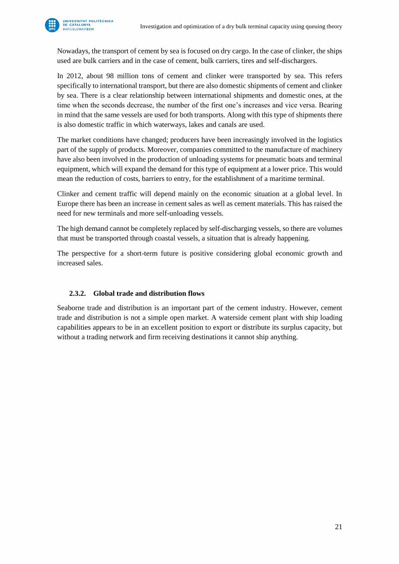
Figure 13. Global seaborne cement and clinker trade flows in 2015. As can be seen in Spain, since 2008, clinker
production is bigger than its consumption when years ago, the situation was the opposite. Source:
https://cementdistribution.com
As can be seen in the figure above, the sea transport of cement and clinker can be configured into
three major types of flows:
1) Regional maritime exports (Atlantic Region, North Region, Middle East Region,
Mediterranean Region, Indian Ocean Region, Northeast Asia Region, Southeast Asia
Region, Caribbean Region), make up approximately 22% of the volume transported.
2) International maritime exports (Intercontinental), being approximately 27% of the total
volume transported.
3) Domestic distribution (USA River System, Great Lakes USA-Canada, coastal and river
transport among others).
Europe is the second-largest exporting area in the world, with the Mediterranean the key export
basis. In 2015 a total of 43.9Mt was exported by sea from European plants, of which 15.3Mt was
traded regionally within the continent, 14Mt was exported to North Africa, 10.7Mt to West Africa
and 3.9Mt to the Americas.
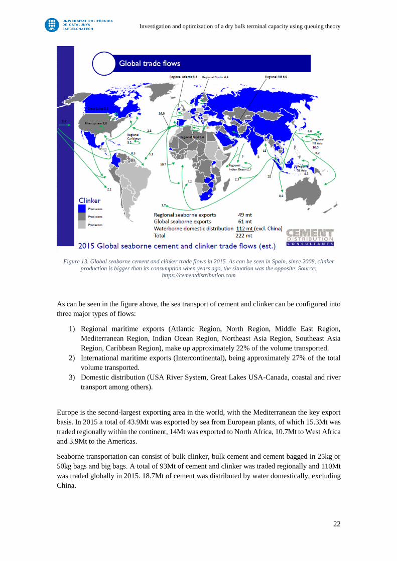
Seaborne transportation can consist of bulk clinker, bulk cement and cement bagged in 25kg or
50kg bags and big bags. A total of 93Mt of cement and clinker was traded regionally and 110Mt
was traded globally in 2015. 18.7Mt of cement was distributed by water domestically, excluding
China.
Investigation and optimization of a dry bulk terminal capacity using queuing theory
23
Figure 14. Clinker and cement trade by water in 2015 in million tons. It is distinguished between seaborne trade
(international and domestic) and inland water domestic trade by type of product. Source:
https://cementdistribution.com
Although China is a large exporter of cement and clinker, it is not an influential country in global
cement trade as it does not own any overseas cement terminals or coastal grinding plants. It
exports because there is a shortage in other markets and its cement is being purchased, but when
that ends, Chinese exports are expected to drop. Chinese cement producers simply do not have
the required large bulk import terminals in these mature markets.
2.4.Overview of cement and clinker in maritime transport
2.4.1. Forms of transportation
The transport of cement by sea focuses on dry cargo. In the case of clinker, the ships used are
bulk carriers and in the case of cement are bulk carriers, tires and self-dischargers. In the case of
packaged cement, it may also be carried out by means of bulk ships and containers. In 2016, about
117 million tons of cement and clinker were transported by sea. There is different type of vessels
for such transports according to the product to be transported. This is especially important since
it gives us an idea of the type of ports that receive these products and the maximum draft of the
terminal determines the type of boat to be used and the regularity of such transports. Of the 3,000
ports that exist worldwide, many of them cannot receive large ships. Self-discharging ships are
mostly used for domestic distribution and short-distance regional trade.

Investigation and optimization of a dry bulk terminal capacity using queuing theory
24
Figure 15. Clinker and cement trade by vessel type in 2015 in million tons. It is distinguished between bulk carriers,
self-discharging cement carriers and inland ships and water barges. Source: https://cementdistribution.com
The table above makes a subdivision of the commodities relating to ship size and type used. It
shows large bulk carriers (Handysize and Handymax), coastal bulk carriers, self-discharging
cement carriers and vessels used for domestic distribution on inland waterways. The fleet of
cement carriers is clearly overstretched. Including small coastal vessels between 500 and
2,000dwt, their total number is about 325. With an average ship size of 7,500dwt and an average
annual tonnage transported of close to 300,000 t/vessel, round-trip times are about a week. The
lower availability of self-discharging vessels in international trade has resulted in growing
shipments in bagged cement and clinker in bulk carriers.
Due to the limits in size and capacity of the buckets, handymax and handysize bulk carriers are
usually the most used.
The global seaborne trade of cement and clinker reached 117 million tons in 2016, and
additionally, another 94 million tons were achieved domestically.
Of all the maritime transport of cement and clinker, approximately 80 million tons were
transported by bulk carriers (handysize and vessels of higher tonnage), 34 million by coastal
vessels and about 97 million by self-discharging cement ships.
2.4.2. Bulk ships
In 2015, a total number of 58 bulk ships carrying cement (26) and clinker (32) were received in
Portcemen Terminal in Port of Barcelona. For these ships, values for the length, the draft, the
beam and the deadweight4, among others, were determined using the databases of Sea-web
(http://www.sea-web.com) and Marinetraffic (http://www.marinetraffic.com). The required quay
length relates to the number and length of the berthed ships that have to be served at the same
time. In Annex C, there is listed an overview of the dimensions determined.
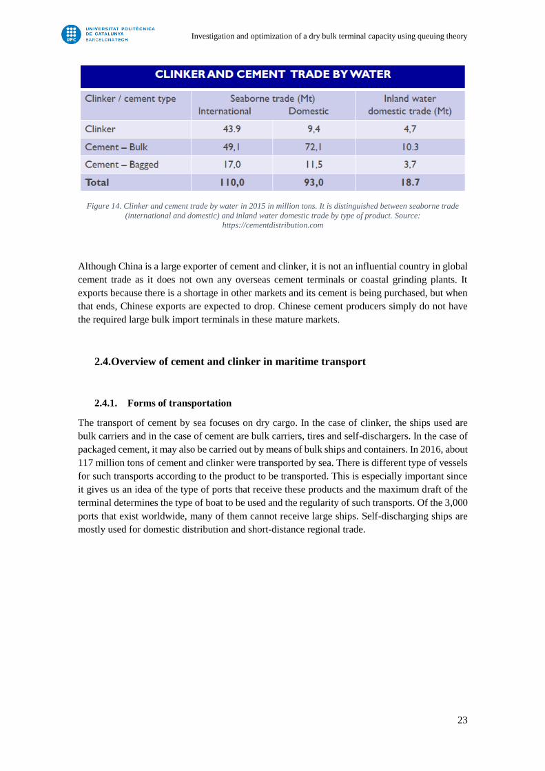
The graphic below shows the relationship between the length of the ship (m) versus its
deadweight1 in tons.
4 The deadweight is the ship’s carrying capacity including the weight of bunkers for fresh water, ballast
water and fuel.
Investigation and optimization of a dry bulk terminal capacity using queuing theory
25
Figure 16. Ship’s length versus the ship’s deadweight. Source: Elaborated by the author based on the databases of
the Sea-web and Marinetraffic.
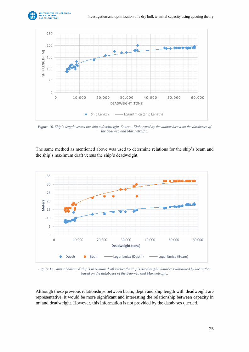
The same method as mentioned above was used to determine relations for the ship’s beam and
the ship’s maximum draft versus the ship’s deadweight.
Figure 17. Ship’s beam and ship’s maximum draft versus the ship’s deadweight. Source: Elaborated by the author
based on the databases of the Sea-web and Marinetraffic.
Although these previous relationships between beam, depth and ship length with deadweight are
representative, it would be more significant and interesting the relationship between capacity in
m3 and deadweight. However, this information is not provided by the databases queried.
0
50
100
150
200
250
0 1 0 . 0 0 0 2 0 . 0 0 0 3 0 . 0 0 0 4 0 . 0 0 0 5 0 . 0 0 0 6 0 . 0 0 0
SHIP
LEN
GTH
(M
)
DEADWEIGHT (TONS)
Ship Length Logarítmica (Ship Length)
0
5
10
15
20
25
30
35
0 10.000 20.000 30.000 40.000 50.000 60.000
Me
ters
Deadweight (tons)
Depth Beam Logarítmica (Depth) Logarítmica (Beam)
Investigation and optimization of a dry bulk terminal capacity using queuing theory
26
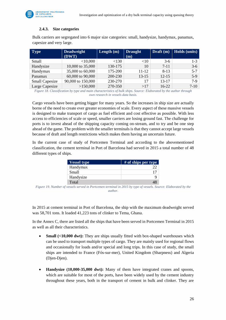
2.4.3. Size categories
Bulk carriers are segregated into 6 major size categories: small, handysize, handymax, panamax,
capesize and very large.
Type Deadweight
(DWT)
Length (m) Draught
(m)
Draft (m) Holds (units)
Small <10,000 <130 <10 3-6 1-3
Handysize 10,000 to 35,000 130-175 10 7-11 3-6
Handymax 35,000 to 60,000 175-200 11-12 8-13 5-7
Panamax 60,000 to 90,000 200-230 13-15 12-15 5-9
Small Capesize 90,000 to 150,000 230-270 17 13-17 7-9
Large Capesize >150,000 270-350 >17 16-22 7-10 Figure 18. Classification by type and main characteristics of bulk ships. Source: Elaborated by the author through
own research in vessels data basis.
Cargo vessels have been getting bigger for many years. So the increases in ship size are actually
borne of the need to create ever greater economies of scale. Every aspect of these massive vessels
is designed to make transport of cargo as fuel efficient and cost effective as possible. With less
access to efficiencies of scale or speed, smaller carriers are losing ground fast. The challenge for
ports is to invest ahead of the shipping capacity coming on-stream, and to try and be one step
ahead of the game. The problem with the smaller terminals is that they cannot accept large vessels
because of draft and length restrictions which makes them having an uncertain future.
In the current case of study of Portcemen Terminal and according to the abovementioned
classification, the cement terminal in Port of Barcelona had served in 2015 a total number of 48
different types of ships.
Vessel type # of ships per type
Handymax 22
Small 17
Handysize 9
Total 48 Figure 19. Number of vessels served in Portcemen terminal in 2015 by type of vessels. Source: Elaborated by the
author.
In 2015 at cement terminal in Port of Barcelona, the ship with the maximum deadweight served
was 58,701 tons. It loaded 41,223 tons of clinker to Tema, Ghana.
In the Annex C, there are listed all the ships that have been served in Portcemen Terminal in 2015
as well as all their characteristics.
Small (<10,000 dwt): They are ships usually fitted with box-shaped warehouses which
can be used to transport multiple types of cargo. They are mainly used for regional flows
and occasionally for loads and/or special and long trips. In this case of study, the small
ships are intended to France (Fós-sur-mer), United Kingdom (Sharpness) and Algeria
(Djen-Djen).
Handysize (10,000-35,000 dwt): Many of them have integrated cranes and spoons,
which are suitable for most of the ports, have been widely used by the cement industry
throughout these years, both in the transport of cement in bulk and clinker. They are

Investigation and optimization of a dry bulk terminal capacity using queuing theory
27
usually used in trips of medium distance. They are also used for the transport of bagged
cement in long-distance trips and in cases of ports with draft restrictions.
Handymax (35,000-60,000 dwt): In the case of this type of ships, they have suffered an
increase in its size in recent years, being currently a large part of the fleet of a size greater
than 55,000dwt. This have been a problem for the cement sector since the maximum
volume is usually between 45,000 and 55,000dwt due to the storage capacity of terminals.
The average storage capacity of most terminals are between 40,000 to 45,000 tons and
which in turn have cement unloaders. This type of ships is mainly used for the transport
of clinker and cement in long-distance routes.
2.4.4. Port facilities
Regarding to maritime trade, the cement industry needs to place its production infrastructures at
a maximum distance of approximately 200km due to it is not economically feasible to export
products away from maritime terminals by sea.
It is necessary to distinguish the infrastructure needed for cement or clinker transport since it is
not used the same loading/unloading machinery due to their physical characteristics.
Referring to clinker, the loading can be done through different systems; by means of the typical
use of cranes and spoons, which can belong to the vessel or to the equipment in ground. It is also
common loading the cargo through cement conveyors.
On the other hand, regarding the loading and discharging methods of cement, we are faced with
two main forms: pneumatic and mechanical machinery. Both technologies allow loading and
unloading the product avoiding dust emissions into atmosphere. Also both methods can be done
from land as well as they can belong to the vessels.
2.4.5. Bulk cement terminals and coastal grinding plants
There are 857 cement terminals around the world who receive cement by sea or inland water
which 169 of them are equipped with a ship unloader and can receive general bulk carriers. A
total of 688 terminals, are served by self-discharging ships. Most of them are used for domestic
distribution or regional trade whereas the ones with a ship unloader are used for international
trade.
Global seaborne cement and clinker trade is controlled by the owners of the exporting and
distributing cement plants, and even more, by the owners of the receiving bulk cement terminals
and grinding facilities.
As can be seen from the table below, the top five multinationals own about 40% of all the facilities
involved in global seaborne trade and distribution.
COMPANY CEMENT
PLANTS
GRINDING
PLANTS
TERMINALS TOTAL
Lafarge 23 16 89 128
Heidelberg Cement 11 19 88 118
Holcim 20 20 77 117

Investigation and optimization of a dry bulk terminal capacity using queuing theory
28
Cemex 19 3 71 93
Italcementi 10 7 21 38
TOTAL 83 (38%) 65 (33%) 34 (40%) 494 (39%) Figure 20. Overview of facilities of the top five multinationals involved in waterborne trade and distribution in 2013.
Cemex (the fourth in the world) is one of the three cement companies that owns Portcemen terminal. Source:
www.cemnet.com.
As it is mentioned before, the Portcemen terminal, the one which is analysed in the current study,
is owned by 3 cement companies which one of them is Cemex. Cemex is one of the biggest
companies in the world in terms of cement transport volumes. As it is seen in the table above, it
has 93 facilities around the world.
2.4.6. Cement terminals
Dry bulk terminals are crucial nodes in the supply chain for the dry bulk products. Two terminal
functions can be distinguished:
- Tranship dry bulk materials between the different transport modalities
- Store the materials temporarily to absorb unavoidable differences in time and quantities
between incoming and outgoing flows.
A dry bulk terminal contains three main subsystems: the seaside, landside and stockyard. The
seaside and landside are the connections with the bulk supply chain where dry bulk materials are
imported to or exported from the terminal.
Dry bulk materials can directly be transferred between the different transport modalities without
being stored at the stockyard. Nevertheless, direct transfer is difficult to realize due to all kind of
interruptions in the bulk supply chain. Most of the cargo is stored for a period of time in piles at
the terminal’s stockyard. Transportation of materials at terminals is generally performed using
belt conveyors as in Portcemen terminal in Port of Barcelona.
In recent years, there has been an increase in cement sales in Europe, and this has raised the need
for new terminals and more self-unloading vessels. On the other hand, new self-discharging ships
have been delivered to northern Europe and this demand will surely increase, considering that due
to the strict environmental policies, it is necessary to replace the old ships.
2.4.7. Required infrastructure in cement terminals
Regarding the required infrastructure in a port for the transport of cement or clinker, it is necessary
to distinguish between both products, since it is used different machinery for each product due to
their physical properties.
In reference to clinker, the loading operation can be done through different systems. By means of
the habitual use of cranes or spoons, which can belong to the ship or to ground-based equipment.
It is also common using cement conveyors for the loading operation.
In the case of cranes and buckets, shippers will have available without any additional cost the use
of the loading and unloading machinery on board, this is usually the most used method.
Furthermore, it has the disadvantage of being the slowest method and at the moment of depositing
Investigation and optimization of a dry bulk terminal capacity using queuing theory
29
the material in the ship’s hold, high emissions of particles are produced in the atmosphere, which
is not appropriate due to the restrictions regarding the emissions.
Regarding the use of cranes and spoons, not being the machinery on board of the ship, implies an
additional cost. It must be borne in mind that the margins of the clinker and cement exportations
are reduced, consequently the stakeholders look for the economical practice. In this case, if the
port has a hopper, it is possible the direct discharge to the truck despite the complexity of this
technique since it is necessary to ensure a constant rate of unloading through the continuous
availability of trucks.
An alternative method used, only in loading operation, is the use of conveyor belts. This system
allows the load through omens made in ship’s hull. Conveyor belts enable the loading in adverse
conditions, as with storms, winds or rains, when it would be impossible to perform with cranes or
spoons.
Regarding the methods of loading and unloading cement, there are two main forms through the
use of pneumatic and mechanical machinery. Both technologies allow the procedure avoiding
dust emissions into the atmosphere.
Both pneumatic and mechanical discharge systems can be combined with different storage
options from domes to silos. Being mechanical discharge system the most versatile in terms of
unloading capacity from different types of ships. However, it has a higher energy consumption
than mechanical unloading systems.
In the case of pneumatic discharge, this is done through the vacuum extraction of the cement from
the holds. The advantage of the machinery is that it is usually more flexible and easier to reach
all the places in the holds when using hoses.
In the case of mechanical unloading, it is carried out by an endless screw. This method is slower
than pneumatic discharge. They usually require systems of transport by conveyor belts until the
storage of the product.
2.4.8. Loading and unloading process
Loading and unloading a bulk carrier is time-consuming and dangerous. All the process is planned
by the ship’s chief mate under the supervision of ship’s captain. The captain and the terminal
master agree on a detailed plan before the operations begin, as it is required in the international
regulations.
Ship-loading equipment
Ship-loading systems are simple in comparison with ship-discharging systems. They normally
require only a feed elevator or conveyor, a loading chute and the force of gravity. With such
technically simple systems, phenomenal rates can be achieved.
Other loaders are fitted with flight conveyors or spiral chutes to reduce the degradation of friable
materials, or with telescopic tubes fitted with chutes or centrifugal slinger belts for distributing
the material in the hold. Ship-loaders can normally be positioned adjacent to the hatch to be
loaded, and they receive the material from high-capacity belt conveyors.

Investigation and optimization of a dry bulk terminal capacity using queuing theory
30
Ship-loader capacities are usually limited by the other parts of the installation such as the
conveyors or reclaimers, but normal capacity ranges are between 1,000 and 7,000 tons an hour.
Figure 21. Example of travelling ship-loader with material from high-level conveyor. Source: Chapter II: Planning
Principles. Port Development: A Handbook for Planners in Developing Countries (UNCTAD)
The ship loading machines used depends on both the cargo and the equipment available on the
ship and on the dock. A widely used method is the double-articulation cranes, which can load at
a rate of 1,000 tons per hour, and the use of shore-based gantry cranes, reaching 2,000 tons per
hour, is growing.
Moreover, conveyor belts offer a really efficient method of loading, with standard rates varying
between 100 and 700 tons per hour. Start-up and shutdown procedures with conveyor belts,
though, are complicates and require time to carry out. Self-discharging ships use conveyor belts
with load rates of approximately 1,000 tons per hour.
Regarding the conveying technologies, screw conveyors are particularly well suited for handling
powdery and dusty materials and where limitations in height need to be considered. A screw-type
loader is thus commonly used for handling commodities such as cement, cement clinker and
combinations of both of them, and is applicable to ships up to Panama size.
It is crucial to keep the cargo level during loading in order to maintain stability. As the hold is
filled, machines such as bulldozers are often used to keep the cargo in check. Levelling is
particularly important when the hold is only partly full, since cargo is more likely to shift.

Investigation and optimization of a dry bulk terminal capacity using queuing theory
31
Figure 22. Functional diagram of cement or clinker loading operations in Portcemen terminal. Source: Duran E.,
Portcemen terminal
Ship-unloading equipment
There exist two types of ship unloading machines for cement and clinker: mobile (rubber tyred or
pontoon mounted) and rail-mounted harbour cranes. Mobile harbour cranes are more flexible but
limited in unloading capacity whereas rail-mounted cranes can only move alongside the quay and
cannot pass each other giving more complexity when dividing over various ships.
A crane’s discharge rate is limited by the bucket’s capacity (from 6 to 40 tons) and by the speed
at which the crane can take a load, deposit it at the terminal and return to take the next. For modern
gantry cranes, the total cycle time is about 50 seconds.
Once the cargo is discharged, it is necessary to clean the holds. This is particularly important if
the next cargo is of a different type. When the holds are clean, the process of loading can start
again.
There are four basic systems available to the terminal operator for the discharge of dry bulk
material: grabs, pneumatic systems, vertical conveyors and bucket elevators. For a throughput per
unit of between 50 and 1,000 tons per hour, pneumatic or vertical conveyor systems are adequate.
For throughputs from 1,000 up to 5,000 tons per hour, grabs or bucket elevators are the only
alternative. Grabs are the most widely used methods of loading and discharging bulk cargoes.
Grabs
The grab is now normally used only for picking material up from the vessel hold and discharging
it into a hopper located at the quay edge feeding on to a belt conveyor. The attainable handling
rate for each grab is determined by the number of handling cycles per hour and the average grab
payload. Grab unloading is the most widely used method for ship unloading.
Investigation and optimization of a dry bulk terminal capacity using queuing theory
32
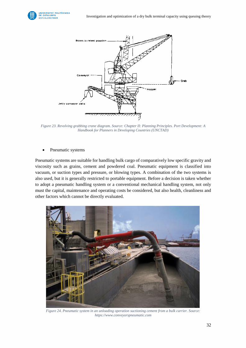
Figure 23. Revolving grabbing crane diagram. Source: Chapter II: Planning Principles. Port Development: A
Handbook for Planners in Developing Countries (UNCTAD)
Pneumatic systems
Pneumatic systems are suitable for handling bulk cargo of comparatively low specific gravity and
viscosity such as grains, cement and powdered coal. Pneumatic equipment is classified into
vacuum, or suction types and pressure, or blowing types. A combination of the two systems is
also used, but it is generally restricted to portable equipment. Before a decision is taken whether
to adopt a pneumatic handling system or a conventional mechanical handling system, not only
must the capital, maintenance and operating costs be considered, but also health, cleanliness and
other factors which cannot be directly evaluated.
Figure 24. Pneumatic system in an unloading operation suctioning cement from a bulk carrier. Source:
https://www.conveyorspneumatic.com
Investigation and optimization of a dry bulk terminal capacity using queuing theory
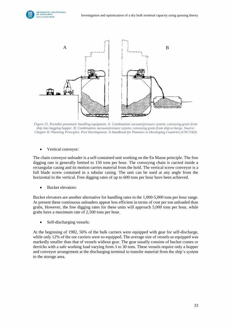
33
Figure 25. Portable pneumatic handling equipment. A: Combination vacuum/pressure system; conveying grain from
ship into bagging hopper. B: Combination vacuum/pressure system; conveying grain from ship to barge. Source:
Chapter II: Planning Principles. Port Development: A Handbook for Planners in Developing Countries (UNCTAD)
Vertical conveyor:
The chain conveyor unloader is a self-contained unit working on the En Masse principle. The free
digging rate is generally limited to 150 tons per hour. The conveying chain is carried inside a
rectangular casing and its motion carries material from the hold. The vertical screw conveyor is a
full blade screw contained in a tubular casing. The unit can be used at any angle from the
horizontal to the vertical. Free digging rates of up to 600 tons per hour have been achieved.
Bucket elevators:
Bucket elevators are another alternative for handling rates in the 1,000-5,000 tons per hour range.
At present these continuous unloaders appear less efficient in terms of cost per ton unloaded than
grabs, However, the free digging rates for these units will approach 5,000 tons per hour, while
grabs have a maximum rate of 2,500 tons per hour.
Self-discharging vessels:
At the beginning of 1982, 56% of the bulk carriers were equipped with gear for self-discharge,
while only 12% of the ore carriers were so equipped. The average size of vessels so equipped was
markedly smaller than that of vessels without gear. The gear usually consists of bucket cranes or
derricks with a safe working load varying from 3 to 30 tons. These vessels require only a hopper
and conveyor arrangement at the discharging terminal to transfer material from the ship’s system
to the storage area.
A B
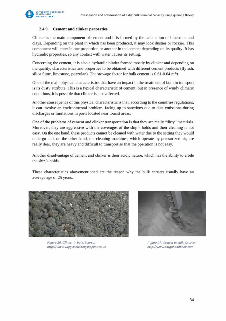
Investigation and optimization of a dry bulk terminal capacity using queuing theory
34
2.4.9. Cement and clinker properties
Clinker is the main component of cement and it is formed by the calcination of limestone and
clays. Depending on the plant in which has been produced, it may look dustier or rockier. This
component will enter in one proportion or another in the cement depending on its quality. It has
hydraulic properties, so any contact with water causes its setting.
Concerning the cement, it is also a hydraulic binder formed mostly by clinker and depending on
the quality, characteristics and properties to be obtained with different cement products (fly ash,
silica fume, limestone, pozzolan). The stowage factor for bulk cement is 0.61-0.64 m3/t.
One of the main physical characteristics that have an impact in the treatment of both in transport
is its dusty attribute. This is a typical characteristic of cement, but in presence of windy climatic
conditions, it is possible that clinker is also affected.
Another consequence of this physical characteristic is that, according to the countries regulations,
it can involve an environmental problem, facing up to sanctions due to dust emissions during
discharges or limitations in ports located near tourist areas.
One of the problems of cement and clinker transportation is that they are really “dirty” materials.
Moreover, they are aggressive with the coverages of the ship’s holds and their cleaning is not
easy. On the one hand, these products cannot be cleaned with water due to the setting they would
undergo and, on the other hand, the cleaning machines, which operate by pressurized air, are
really dear, they are heavy and difficult to transport so that the operation is not easy.
Another disadvantage of cement and clinker is their acidic nature, which has the ability to erode
the ship’s holds.
These characteristics abovementioned are the reason why the bulk carriers usually have an
average age of 25 years.
Figure 26. Clinker in bulk. Source:
http://www.wigginsbuildingsupplies.co.uk
Figure 27. Cement in bulk. Source:
http://www.cargohandbook.com

Investigation and optimization of a dry bulk terminal capacity using queuing theory
35
2.5.Description of the data
The analysis of the cement terminal in Barcelona Port has been based on the data provided by
Portcemen terminal. These data included all vessels calls in this terminal during the year 2015. In
total, 58 bulk carriers were served in Portcemen terminal, on average, 5 vessels per month.
It is necessary to assume the random nature of the arrivals in case of non-programmed calls.
Although the larger vessels (such as handysize or handymax) have scheduled arrivals, the smaller
ones do not. In this case, when they arrive at the port, if the terminal is free, they can be served at
the same time.
It should also be considered that the duration of the calls is not fixed, but dependent on the amount
of cement and clinker to be loaded. Moreover, the crane performance sets the duration of the
service.
Loading performance of clinker 1,100 tons/h
Loading performance of cement 500 tons/h
When the arrivals are independent of the number of customers in the system, it is considered an
infinite-source model, resulting a mathematically tractable model.
For this minor thesis, it is assumed that data follows a stochastic model, also known as
probabilistic model, which some factors are not known in advanced, thus incorporating
uncertainty. Nevertheless, in reality, other types of models are used such as deterministic models.
They are those where it is assumed that the data are known with certainty, that is, it is assumed
that when the model is analyzed all the necessary information for decision making is available.
A stochastic process uses random magnitudes that vary with time or characterize a succession of
random (stochastic) variables that evolve based on another variable, usually time. Each of the
random variables in the process has its own probability distribution function and may or may not
be correlated with each other. Moreover, the process follows the Márkov property5, or
memoryless, which means that the probability distribution of the future value of a random variable
only depends on its present value, being independent of the history of said variable.
To sum up, although in reality vessels arrivals are considered as deterministic models, for this
minor thesis it is considered as a stochastic model which we assume that arrivals are random. In
addition, these arrivals only depend on the current state of the system (neither previous nor next).
In order to preserve the data confidentiality, the detailed information of the arrivals in Portcemen
Terminal has not been shown in this document.
5 The term Markov property refers to the memoryless property of a stochastic process. It is named after the
Russian mathematician Andrey Markov.

Investigation and optimization of a dry bulk terminal capacity using queuing theory
36
3. METHODS
3.1.Queuing theory
A huge number of application research shows that queuing theory6 is one of the effective methods
to solve the optimization of system operation parameter in addition to find the most economic
system operation cost. Also, queueing theory is generally considered as a branch of operational
research became the resources needed to provide service. Then queueing theory is an application
of stochastic processes in operations research.
The queuing phenomenon is widely disseminated in the field of logistics handling, such as how
to design the pier berth, how to purchase the handling equipment, etc., and how to not only satisfy
the arrival in punctual service demand but also design the best configuration scheme possible for
the berth, handling equipment and service resources under the condition of saving port resources.
Although it does not solve all types of waiting line problems, it provides useful and vital
information by forecasting or predicting multiple characteristics and parameters of the particular
waiting line under study.
Since the predictions about the waiting times, the time for which the server remain busy, etc. rely
on the basic concept of stochastic processes, it can very well be taken as an application of
stochastic processes.
Cargo vessels arrive at the ports, and wait for the process of handling services. It can also be seen
as a queuing process, the vessels are equivalent to the customers, the handling facilities are
equivalent to servers.
Figure 28. Queuing System Diagram. Source: Elaborated by the author.
The figure describes each vessel reach the port, first, join the queue and wait for handling services.
Servers select the ships to load and unload from the queue in certain rules, then the vessels after
being served, left.
The basic queuing system can be extended to a queuing system of variety of queuing methods.
There are three main concepts in queueing theory, which are queue (waiting line), customer and
server. The queueing theory is the probabilistic study of waiting lines.
6 Queueing theory has its origins in research by Agner Krarup Erlang when he created models to describe
the Copenhagen telephone exchange.

Investigation and optimization of a dry bulk terminal capacity using queuing theory
37
3.1.1. Fundamentals
Queuing theory involves the mathematical study of queues, or waiting lines. The waiting
phenomenon is the direct result of randomness in operation of service facility, and customer’s
arrivals.
The following are the six basis characteristics of a queueing system. They are explained below.
Arrival pattern of customers
Service pattern of servers
Queue discipline
System capacity
Service channels
Stages of service
The principal’s elements in a queuing situation are the customer (ship) and the server (handling
equipment). In queuing models, customer arrivals and service times are expressed in terms of
probability distributions normally referred to as arrivals and service time distributions that fit the
pattern of time difference between two consecutive arrivals. Generally, the arrival of clients can
be defined as a stochastic process.
Figure 29. Ship queue at the seaport diagram. Source: Elaborated by the author.
─ Arrival pattern of customers
The arrival process consists of describing how customers arrive to the system. The system may
have either a limited or an unlimited capacity for holding units. The source from which the units
come may be finite or infinite.
The interval between two consecutive arrivals is called the inter-arrival time. The arrival pattern
of a system is measured in terms of the average number of arrivals per unit time (mean arrival
rate) or by the average time between successive arrivals (mean inter-arrival time). In queueing

Investigation and optimization of a dry bulk terminal capacity using queuing theory
38
theory, the inter-arrival times and the services times (sometimes it is called service request) are
usually assumed to be independent and identically distributed random variables.
If the arrival pattern is deterministic, then it is fully determined by either the mean arrival rate or
the mean inter-arrival time. On the other hand, if it is probabilistic, then further characterization
is required in the form of the probability distribution associated with the random process. If the
arrival pattern does not change with time, then it is called a stationary arrival pattern, otherwise,
it is called non-stationary.
Another factor to be considered regarding the arrival pattern is the reaction of the customers in
the queue. If the queue is too long, a customer may decide not to enter it upon arrival and in this
situation he is said to have balked. On the other hand, a customer may enter the queue but after
some time lose patience and decide to leave. In this case, he is said to have reneged.
In many studies, analytical distributions were applied to represent the ship inter-arrival times. The
table below presents an overview of these suggested distributions. When distributions were
derived from real-world data, the number of ships (ns) is listed in the table.
Figure 30. Overview of proposed inter-arrival time distributions (IATDist). For dry bulk cargo, it proposes Weibull,
Erlang-2 and negative exponential (NED) distributions. Source: Van Vianen, T., Simulation-Integrated Design of Dry
Bulk Terminals
As referred in the PhD thesis Simulation-Integrated Design of Dry Bulk Terminals (Van Vianen,
T., 2015), most papers used the negative exponential distribution (NED) to represent the ship
inter-arrival times. The arrival process can then be represented by a Poisson arrival process. The
ships arrive randomly and independently. The proposed NED distribution for container terminals
is remarkable. At container terminals, ship arrivals are scheduled and therefore expected not
random. However, Pachakis and Kiremidjian (2003) stated that the superposition of several
independent container shipping lines with uniformly arrival rates yields approximately a Poisson
arrival pattern.

Investigation and optimization of a dry bulk terminal capacity using queuing theory
39
In this thesis, Kolmogorov-Smirnov test is used for curve fitting between measured and analytical
distributions (See Chapter 4).
─ Service pattern of servers
Service pattern can be described by the number of services per unit time (service rate) or by the
time required to service customer (service time). Service may also be in single or in batch, further
it can be stationary or non-stationary. One important difference between arrival and service is that
service rate or service time are conditioned on the fact that the system is not empty. If the system
is empty, the server is idle.
For both of the characteristics abovementioned, although their pattern could change in time, it
will be considered as stationary. The time needed to load or unload ships is called the ship service
time (Ws).
The handling of containers at the terminal’s seaside has similarities with bulk ship unloading; in
each crane cycle a container is handled or a certain tons of material is unloaded from the hold.
Other similarities are that the handling capacity per crane reduces when multiple cranes are
deployed at a ship and the crane cycle time increases when the ship becomes more emptied.
The table below lists an overview of proposed service time distributions for both container and
dry bulk cargo. When distributions were derived from real-world data, the number of ships (ns) is
listed in the table.
Figure 31. Overview of proposed service time distributions (WsDist). For dry bulk cargo, it proposes Normal,
Gamma and Erlang-k distributions. Source: Van Vianen, T., Simulation-Integrated Design of Dry Bulk Terminals
In the PhD thesis Simulation-Integrated Design of Dry Bulk Terminals (Van Vianen, T., 2015),
several proposed service time distributions were compared with the measured service time
distributions from three dry bulk terminals. The chi-square method was used to fit these measured
distributions with one of the analytical distributions proposed for dry bulk terminals (Erlang-k,
Normal and Gamma). All three service time distributions show the best fit with an Erlang-2
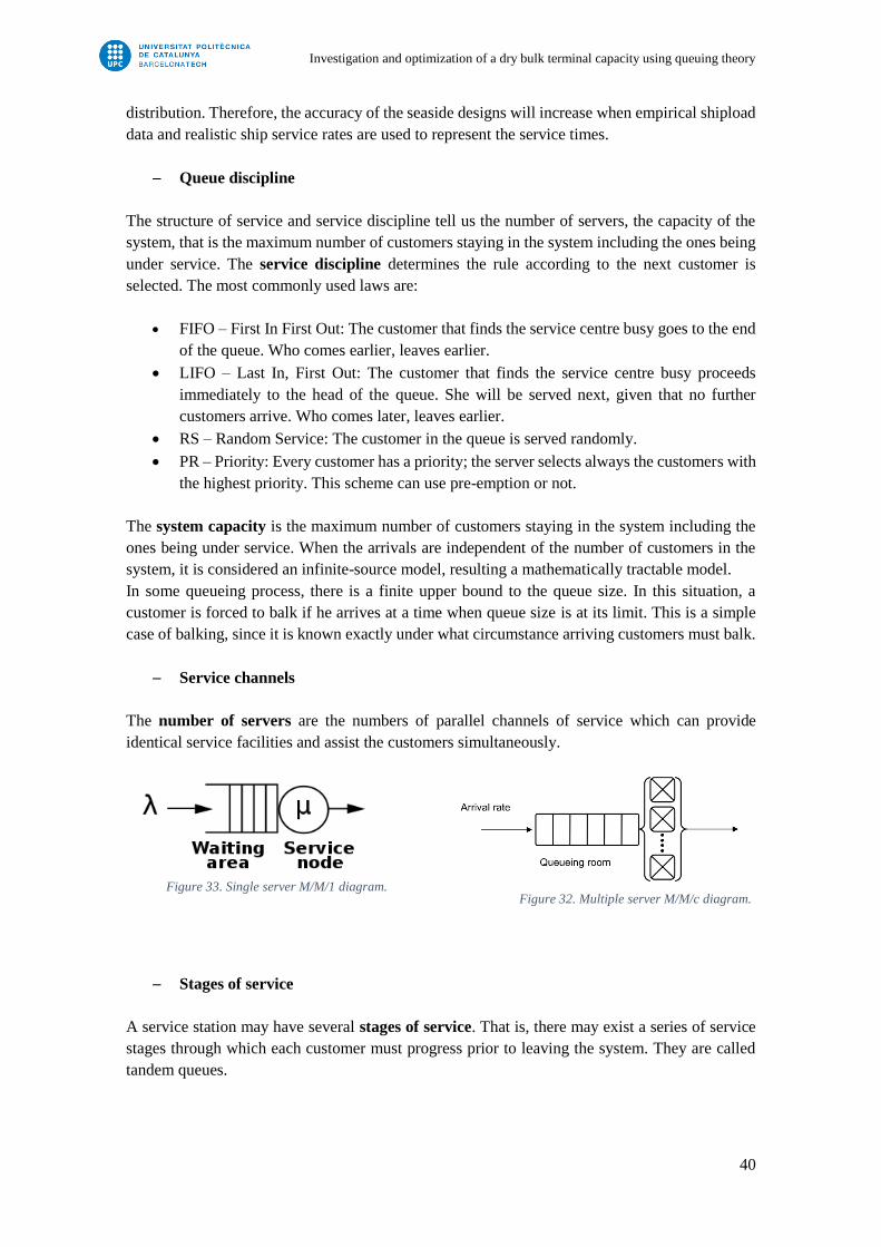
Investigation and optimization of a dry bulk terminal capacity using queuing theory
40
distribution. Therefore, the accuracy of the seaside designs will increase when empirical shipload
data and realistic ship service rates are used to represent the service times.
─ Queue discipline
The structure of service and service discipline tell us the number of servers, the capacity of the
system, that is the maximum number of customers staying in the system including the ones being
under service. The service discipline determines the rule according to the next customer is
selected. The most commonly used laws are:
FIFO – First In First Out: The customer that finds the service centre busy goes to the end
of the queue. Who comes earlier, leaves earlier.
LIFO – Last In, First Out: The customer that finds the service centre busy proceeds
immediately to the head of the queue. She will be served next, given that no further
customers arrive. Who comes later, leaves earlier.
RS – Random Service: The customer in the queue is served randomly.
PR – Priority: Every customer has a priority; the server selects always the customers with
the highest priority. This scheme can use pre-emption or not.
The system capacity is the maximum number of customers staying in the system including the
ones being under service. When the arrivals are independent of the number of customers in the
system, it is considered an infinite-source model, resulting a mathematically tractable model.
In some queueing process, there is a finite upper bound to the queue size. In this situation, a
customer is forced to balk if he arrives at a time when queue size is at its limit. This is a simple
case of balking, since it is known exactly under what circumstance arriving customers must balk.
─ Service channels
The number of servers are the numbers of parallel channels of service which can provide
identical service facilities and assist the customers simultaneously.
Figure 33. Single server M/M/1 diagram.
─ Stages of service
A service station may have several stages of service. That is, there may exist a series of service
stages through which each customer must progress prior to leaving the system. They are called
tandem queues.
Figure 32. Multiple server M/M/c diagram.

Investigation and optimization of a dry bulk terminal capacity using queuing theory
41
The aim of all investigations in queueing theory is to get the main performance measures of the
system which are the probabilistic properties (distribution function, density function, mean,
variance) of the following random variables: number of customers in the system, number of
waiting customers, utilization of the server/s, response time of a customer, waiting time of a
customer, idle time of the server, busy time of a server. Of course, the answers heavily depend on
the assumptions concerning the distribution of inter-arrival times, service times, number of
servers, system’s capacity and service discipline.
Kendall’s notation
The Kendall Notation is used for a short characterization of queueing systems. A queueing system
description is described by the following notation:
A / B / m / K / n / D
Where:
A denotes the distribution function of the inter-arrival times
B denotes the distribution function of the service times
m denotes the number of service channels. The M/M/1 queue has a single server and the
M/M/c queue has c servers.
K denotes the capacity of the system, the maximum number of customers allowed in the
system including those being serviced. When the number is at this maximum, further
arrivals are turned away. If this number is omitted, the capacity is assumed to be
unlimited, or infinite.
n denotes the population size. If this number is omitted, the population is assumed to be
unlimited, or infinite.
D denotes the service discipline (FIFO, LIFO, RS, PR, etc.). If it is omitted, the service
discipline is always FIFO.
For the values of A and B, the following abbreviations are generally applied:
M (Markovian Process): This denotes the exponential distribution. The name M stems
from the fact that the exponential distribution is the only continuous distribution with the
markov property (memoryless).
D (Deterministic): All values from deterministic “distribution” are constant (have the
same value).
Ek (Erlang-k): Erlang Distribution with k phases (k≥1)
Hk (Hyper-k): Hyperexponential distribution with k phases
G (General): General distribution. In most cases at least the mean and the variance are
known.

Investigation and optimization of a dry bulk terminal capacity using queuing theory
42
Little’s Law
Little’s law7 is a theorem by John Little which establishes a relationship between the average
number of customers in the system, the mean arrival rate and the mean time between entering and
leaving the system in the steady state.
Expressed algebraically the law is:
𝑁 = 𝜆 · 𝑊
Where,
N = Average number of customers in the system
λ = Mean arrival rate of clients that enter the system
W = Average time that a client spends in the system
This relationship applies to all systems or parts of systems in which the number of clients entering
the system is equal to those completing service. The only requirements are that the system be
stable and non-preemptive.
Little’s theorem does not assume any specific distribution for the arrivals as well as the service
process and any queuing discipline. Also, it does not depend upon the number of parallel servers
in the system. The theorem can be applied to all types of queuing systems as long as the servers
kept busy when the system is not empty.
7 In a 1954 paper Little's law was assumed true and used without proof. The form L = λW was first published
by Philip M. Morse where he challenged readers to find a situation where the relationship did not hold.
Little published in 1961 his proof of the law, showing that no such situation existed. Little's proof was
followed by a simpler version by Jewell and another by Eilon. Shaler Stidham published a different and
more intuitive proof in 1972. Graves, S. C. (2008). "Little's Law" Building Intuition.
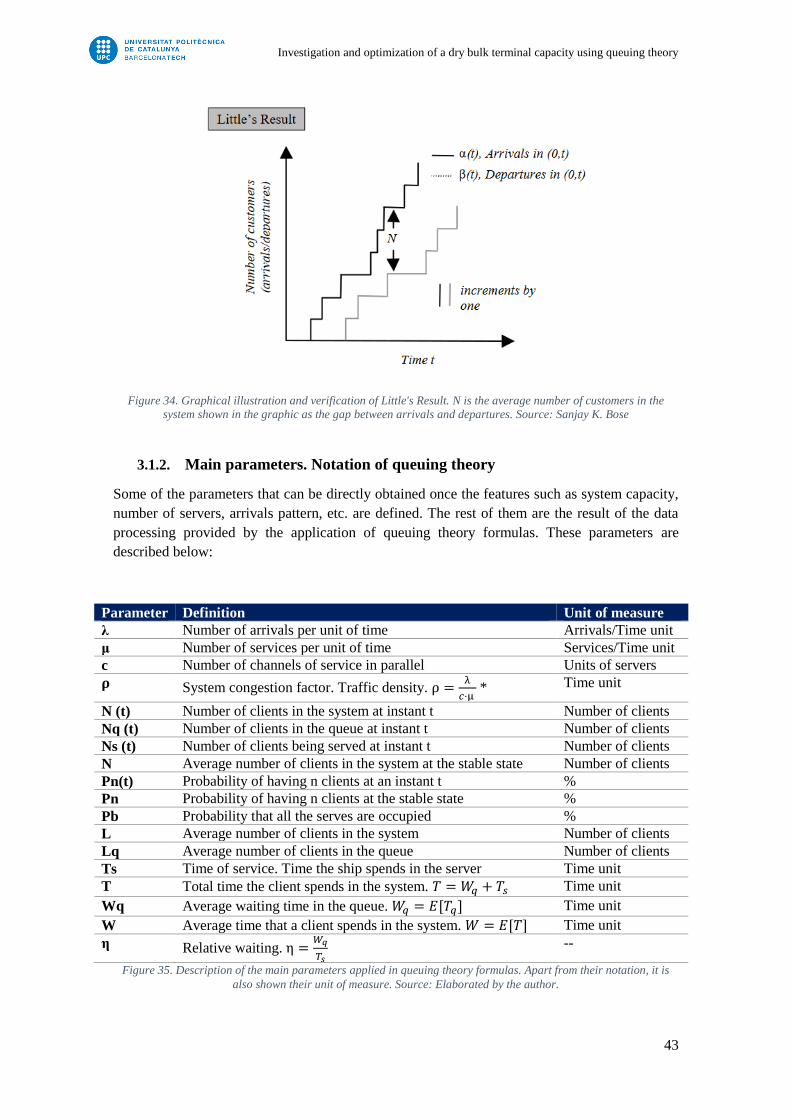
Investigation and optimization of a dry bulk terminal capacity using queuing theory
43
Figure 34. Graphical illustration and verification of Little's Result. N is the average number of customers in the
system shown in the graphic as the gap between arrivals and departures. Source: Sanjay K. Bose
3.1.2. Main parameters. Notation of queuing theory
Some of the parameters that can be directly obtained once the features such as system capacity,
number of servers, arrivals pattern, etc. are defined. The rest of them are the result of the data
processing provided by the application of queuing theory formulas. These parameters are
described below:
Parameter Definition Unit of measure
λ Number of arrivals per unit of time Arrivals/Time unit
μ Number of services per unit of time Services/Time unit
c Number of channels of service in parallel Units of servers
𝛒 System congestion factor. Traffic density. ρ =λ
𝑐·μ * Time unit
N (t) Number of clients in the system at instant t Number of clients
Nq (t) Number of clients in the queue at instant t Number of clients
Ns (t) Number of clients being served at instant t Number of clients
N Average number of clients in the system at the stable state Number of clients
Pn(t) Probability of having n clients at an instant t %
Pn Probability of having n clients at the stable state %
Pb Probability that all the serves are occupied %
L Average number of clients in the system Number of clients
Lq Average number of clients in the queue Number of clients
Ts Time of service. Time the ship spends in the server Time unit
T Total time the client spends in the system. 𝑇 = 𝑊𝑞 + 𝑇𝑠 Time unit
Wq Average waiting time in the queue. 𝑊𝑞 = 𝐸[𝑇𝑞] Time unit
W Average time that a client spends in the system. 𝑊 = 𝐸[𝑇] Time unit
η Relative waiting. η =𝑊𝑞
𝑇𝑠 --
Figure 35. Description of the main parameters applied in queuing theory formulas. Apart from their notation, it is
also shown their unit of measure. Source: Elaborated by the author.

Investigation and optimization of a dry bulk terminal capacity using queuing theory
44
*The system congestion factor represents the relation between the arrivals and the capacity of the
system. If μ> λ, then there is the possibility that a queue is generated so the system is not capable
of satisfy the demand. In contrast, if μ< λ, there is the possibility that the system is over
dimensioned.
In pursuit of these parameters, it is necessary to distinguish the different probabilistic models
which are applied in each case.
Down below, it is shown a diagram with the relationships between the parameters
abovementioned.
Figure 36. Representation of the relationships between the main parameters of queuing theory based on the waiting
area and the service node. Source: University of Pittsburg.
3.1.3. Modelling ship arrival process
The most common arrival pattern of ships in a seaport are the random and scheduled arrivals with
considerable delays. Thus, to predict the number of ships that arrive in a port in a certain time of
period, the arrival pattern of ships may be approximated by a Poisson function8 (See Chapter 4).
The Poisson distribution is defined as:
𝑃(𝑛, λ) =λ𝑛 · 𝑒−λ
𝑛!
Where,
P (n, λ) = Probability of the arrival of k ships in the port in a given time
λ = Average arrival rate of n ships during the given time
e = Base of natural logarithm (e=2.718289…)
n! = Factorial of ship number
8 The Poisson Distribution, named after French mathematician Siméon Denis Poison, is a discrete
probability distribution that expresses the probability of a given number of events occurring in a fixed
interval of time or space if these events occur with a known constant rate and independently of the time
since the last event.

Investigation and optimization of a dry bulk terminal capacity using queuing theory
45
The time between arrivals is defined, in this way, as the probability that no client arrives:
𝑝0(𝑡) = 𝑒−𝜆𝑡
being therefore an exponential distribution.
The expected value and variance are:
𝐸(𝑋) = 𝑉𝑎𝑟(𝑋) = 𝜆
The distribution of ships arrivals with Poisson function can be calculated only if the average
arrival rate during the entire period is known. The expected frequency 𝐹𝑛 of n ships in port in a
given time T is:
𝐹𝑛 = 𝑇 · 𝑃(𝑛,λ)
3.1.4. Modelling inter-arrival time
It is assumed that the ships arrival follows a Poisson process. The inter-arrival times are modelled
as continuous variables. Therefore, the time between two consecutive arrivals can be adjusted to
an Exponential Distribution9 (See Chapter 4):
𝑓(𝑥) = 𝑃(𝑥) = {𝜆𝑒−𝜆𝑥, 𝐹𝑜𝑟 𝑥 ≥ 00, 𝐼𝑛 𝑜𝑡ℎ𝑒𝑟 𝑐𝑎𝑠𝑒
The Cumulative Distribution Function (CDF) will be:
𝐹(𝑥) = 𝑃(𝑋 ≤ 𝑥) = {0, 𝐹𝑜𝑟 𝑥 < 0
1 − 𝑒−𝜆𝑥, 𝐹𝑜𝑟 𝑥 ≥ 0
The expected value and variance are:
𝐸[𝑋] =1
𝜆 𝑉𝑎𝑟[𝑋] =
1
𝜆2
9 The exponential distribution (also known as negative exponential distribution) is the probability
distribution that describes the time between events in a Poisson point process, i.e., a process in which events
occur continuously and independently at a constant average rate. It is a particular case of the gamma
distribution. It is the continuous analogue of the geometric distribution, and it has the key property of being
memoryless.
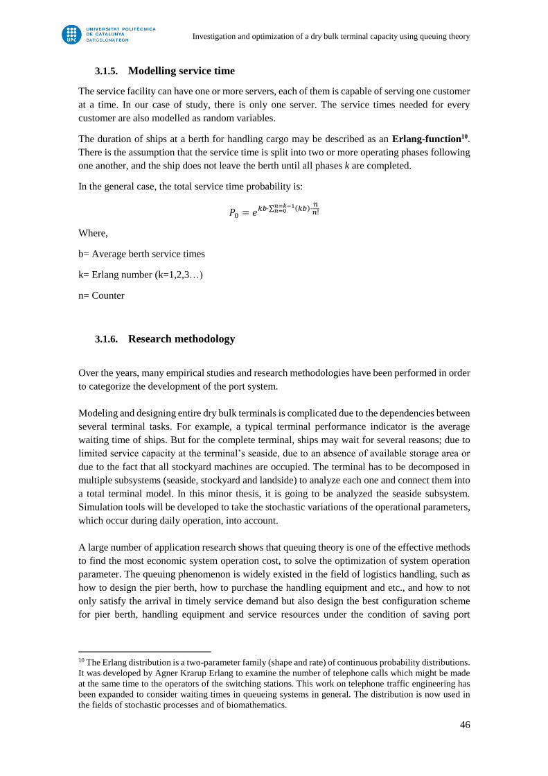
Investigation and optimization of a dry bulk terminal capacity using queuing theory
46
3.1.5. Modelling service time
The service facility can have one or more servers, each of them is capable of serving one customer
at a time. In our case of study, there is only one server. The service times needed for every
customer are also modelled as random variables.
The duration of ships at a berth for handling cargo may be described as an Erlang-function10.
There is the assumption that the service time is split into two or more operating phases following
one another, and the ship does not leave the berth until all phases k are completed.
In the general case, the total service time probability is:
𝑃0 = 𝑒𝑘𝑏·∑ (𝑘𝑏)·𝑛𝑛!
𝑛=𝑘−1𝑛=0
Where,
b= Average berth service times
k= Erlang number (k=1,2,3…)
n= Counter
3.1.6. Research methodology
Over the years, many empirical studies and research methodologies have been performed in order
to categorize the development of the port system.
Modeling and designing entire dry bulk terminals is complicated due to the dependencies between
several terminal tasks. For example, a typical terminal performance indicator is the average
waiting time of ships. But for the complete terminal, ships may wait for several reasons; due to
limited service capacity at the terminal’s seaside, due to an absence of available storage area or
due to the fact that all stockyard machines are occupied. The terminal has to be decomposed in
multiple subsystems (seaside, stockyard and landside) to analyze each one and connect them into
a total terminal model. In this minor thesis, it is going to be analyzed the seaside subsystem.
Simulation tools will be developed to take the stochastic variations of the operational parameters,
which occur during daily operation, into account.
A large number of application research shows that queuing theory is one of the effective methods
to find the most economic system operation cost, to solve the optimization of system operation
parameter. The queuing phenomenon is widely existed in the field of logistics handling, such as
how to design the pier berth, how to purchase the handling equipment and etc., and how to not
only satisfy the arrival in timely service demand but also design the best configuration scheme
for pier berth, handling equipment and service resources under the condition of saving port
10 The Erlang distribution is a two-parameter family (shape and rate) of continuous probability distributions.
It was developed by Agner Krarup Erlang to examine the number of telephone calls which might be made
at the same time to the operators of the switching stations. This work on telephone traffic engineering has
been expanded to consider waiting times in queueing systems in general. The distribution is now used in
the fields of stochastic processes and of biomathematics.
Investigation and optimization of a dry bulk terminal capacity using queuing theory
47
resources. So applying queuing theory and method to solve the optimization of port handling
service system is of important theoretical and practical significance.
Over the years, many empirical studies and research methodologies have been performed in order
to categorize the development of the port system. Ducruet, C. (2013) proposes an analysis of
worldwide inter-port shipping flows from a strength-clustering perspective. A variety of factors
seem to explain the formation of clusters: geographic proximity among closely located ports, trade
proximity and historical path-dependency among more distant ports.
A huge number of application research shows that queuing theory is one of the effective methods
to solve the optimization of system operation parameter in addition to find the most economic
system operation cost. Roes, P. B. M. (1966) prove in this study “Operations Research” the theory
of derived Markov chains applied to a queuing system with n servers and group service. The same
methodology was applied by Harris, C. M. (1970) proving it in bulk-arrival queues with state
dependent service times. Accordingly, Hess, M. et al (2007) demonstrates the application of the
queuing theory in modelling the port's bulk cargo unloading terminal on the basis of a bulk cargo
terminal observation as a queuing system defined by basic parameters: the rate of bulk cargo ship
arrivals or quantity of bulk cargo and the rate of ship servicing i. e. quantity of bulk cargo, in an
observed time unit.
Moreover, Bugaric, U., et al. (2007) prove that work of the terminals with its optimal capacity
assumes prompt accommodation of vessels with minimal waiting time in the port and with
maximal use of berth facilities, i.e. bigger unloading capacity. A simulation model of the terminal
work with strategy is developed. Some of the obtained results are applied and verified on existing
system.
Regarding dry bulk terminals, Van Vianen, T.A. et al (2012) focus their paper on route selection
to transport the materials. Due to several sources of uncertainty, selecting routes is complicated
and is now predominately based on the human operators' experiences. A decision support system,
so-called Dynamic Planner, is proposed which consists of a primary simulation model, that
simulates the dynamics of the terminal, and within this primary simulation model, a secondary
simulation model that simulates and proposes routes.
In this direction, Wadhwa, L. C. (2000) in his study deals with finding an optimal solution to an
interesting situation where using one shiploader results in unacceptable ship waiting times and a
high level of demurrage, whereas continuous deployment of two shiploaders results in
inefficiency and high operating costs. So this paper describes an approach for developing a
strategy that considers a trade-off between the ship waiting cost and the cost of deploying the
additional shiploader and results in the optimal deployment of resources.
All of these research methodologies have been used to solve the optimization of port handling
service system. These methodologies are widely used in the current literature, specifically, the
queuing theory and simulation scenarios.
Investigation and optimization of a dry bulk terminal capacity using queuing theory
48
3.2.M/M/1
The type of vessels queuing is the key to establish a fine handling queuing system, making the
operation of handling queuing system unproblematic. According to the characteristics of handling
in the ports and ships as well as a great deal of statistics data, it can be shown that, in most queuing
systems for handling service, the arrival of the ships follows the Poisson distribution while the
time for handling service follows the negative exponential distribution.
In normal circumstances, improving service levels and increasing the number of servers, can
improve the service efficiency and reduce the waiting time. However, improving the level of
service and increasing the number of servers will increase the service costs too. Therefore, to
achieve the purpose of optimization, we must make the sum of service cost and waiting cost to be
minimal.
To analyse the movement of the ships using the queuing theory, the following conditions are
assumed:
i. Ships arrivals and service times comply with the pattern of random occurrences.
ii. Ships are processed on the FIFO queue discipline.
iii. The queue length is unlimited, that is, if a ship arrives and finds a long queue, it joins
the waiting ships and does not leave the port.
Thus, the most typical queuing system is the M/M/111 which can be described as:
- A single server
- No restriction on the capacity of the system and infinite waiting line
- FIFO discipline
- Customer inter-arrival times are identically and exponentially distributed with parameter λ.
They are determined by a Poisson process.
- Customer service times are identically and exponentially distributed with parameter μ.
They are determined by an exponential distribution.
Exponentially distributed random variables are notated by M, meaning Markovain or
memoryless. Furthermore, if the population size and the capacity is infinite, the service discipline
is FIFO, then they are omitted. What makes the M/M/1 system really simple is that the arrival
rate and the service rate are not state-dependent.
Customers arrive according to a Poisson process with exponentially distributed inter-
arrival times (IAT).
𝑃(𝐼𝐴𝑇 ≤ 𝑡) = 1 − 𝑒−𝜆𝑡, 𝑚𝑒𝑎𝑛 𝑖𝑛𝑡𝑒𝑟𝑎𝑟𝑟𝑖𝑣𝑎𝑙 𝑡𝑖𝑚𝑒 =1
𝜆
Customers are served by a single server with exponential service time distribution P.
11 Morse (1955) studied the M/M/1 queue and obtained the transient state probabilities of the number in the
system at time t. The problem was studied and a complete solution was obtained in the 1950's by several
researchers using different methods. The steady state behavior of the queueing system was primarily
investigated by Erlang (1917) and he obtain the steady state probabilities for M/M/1/infinite. The main
limitation observed in the steady state distribution is that there may exist many stochastic processes with
the same stationary distribution.
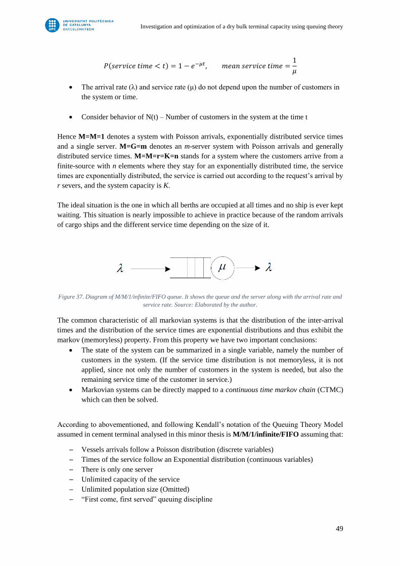
Investigation and optimization of a dry bulk terminal capacity using queuing theory
49
𝑃(𝑠𝑒𝑟𝑣𝑖𝑐𝑒 𝑡𝑖𝑚𝑒 < 𝑡) = 1 − 𝑒−𝜇𝑡, 𝑚𝑒𝑎𝑛 𝑠𝑒𝑟𝑣𝑖𝑐𝑒 𝑡𝑖𝑚𝑒 =1
𝜇
The arrival rate (λ) and service rate (μ) do not depend upon the number of customers in
the system or time.
Consider behavior of N(t) – Number of customers in the system at the time t
Hence M=M=1 denotes a system with Poisson arrivals, exponentially distributed service times
and a single server. M=G=m denotes an m-server system with Poisson arrivals and generally
distributed service times. M=M=r=K=n stands for a system where the customers arrive from a
finite-source with n elements where they stay for an exponentially distributed time, the service
times are exponentially distributed, the service is carried out according to the request’s arrival by
r severs, and the system capacity is K.
The ideal situation is the one in which all berths are occupied at all times and no ship is ever kept
waiting. This situation is nearly impossible to achieve in practice because of the random arrivals
of cargo ships and the different service time depending on the size of it.
Figure 37. Diagram of M/M/1/infinite/FIFO queue. It shows the queue and the server along with the arrival rate and
service rate. Source: Elaborated by the author.
The common characteristic of all markovian systems is that the distribution of the inter-arrival
times and the distribution of the service times are exponential distributions and thus exhibit the
markov (memoryless) property. From this property we have two important conclusions:
The state of the system can be summarized in a single variable, namely the number of
customers in the system. (If the service time distribution is not memoryless, it is not
applied, since not only the number of customers in the system is needed, but also the
remaining service time of the customer in service.)
Markovian systems can be directly mapped to a continuous time markov chain (CTMC)
which can then be solved.
According to abovementioned, and following Kendall’s notation of the Queuing Theory Model
assumed in cement terminal analysed in this minor thesis is M/M/1/infinite/FIFO assuming that:
─ Vessels arrivals follow a Poisson distribution (discrete variables)
─ Times of the service follow an Exponential distribution (continuous variables)
─ There is only one server
─ Unlimited capacity of the service
─ Unlimited population size (Omitted)
─ “First come, first served” queuing discipline
Investigation and optimization of a dry bulk terminal capacity using queuing theory
50
4. RESULTS
4.1.Current situation
This chapter explains the current situation of the terminal with detailed information about the
assumptions done, the calculations of the parameters for the selected queuing model, a manual
simulation with the data provided and the calculations of the levels of service.
4.1.1. Sources of the data
The analysis of the cement terminal in Barcelona Port has been based on the data provided by
Portcemen terminal. These data included all the vessel calls in this terminal during the year 2015.
Specifically, the information provided included the following details:
- Sequence
- Cargo type (cement or clinker)
- Date
- Vessel name
- Destination
- Metric tons
There was some data that was missing in the information provided by the terminal. For example,
there were few calls which didn’t have date. In these cases, an extrapolation of data has been
carried out to complete the information.
In order to preserve the data confidentiality, the detailed arrivals have not been showed in the
present document. The only information that can be found in the document is the date of the calls,
but not the vessel, the type of cargo that carries nor the volume to load or unload. The
characteristics of the vessels that were served in Portcemen terminal are listed in Annex C and D
in alphabetic order, but are not associated to any traffic. The information displayed in this
document came from Barcelona Port Authority, PORTIC, Sea-Web, Marinetraffic and
Vesselfinder.
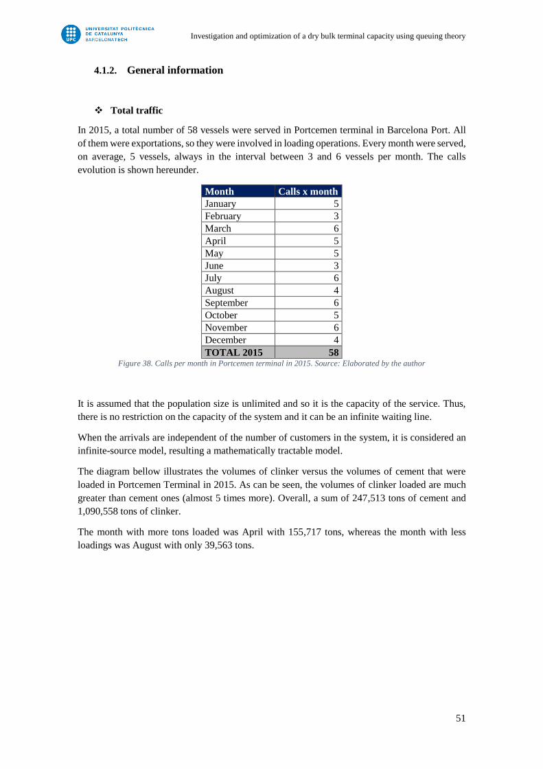
Investigation and optimization of a dry bulk terminal capacity using queuing theory
51
4.1.2. General information
Total traffic
In 2015, a total number of 58 vessels were served in Portcemen terminal in Barcelona Port. All
of them were exportations, so they were involved in loading operations. Every month were served,
on average, 5 vessels, always in the interval between 3 and 6 vessels per month. The calls
evolution is shown hereunder.
Month Calls x month
January 5
February 3
March 6
April 5
May 5
June 3
July 6
August 4
September 6
October 5
November 6
December 4
TOTAL 2015 58 Figure 38. Calls per month in Portcemen terminal in 2015. Source: Elaborated by the author
It is assumed that the population size is unlimited and so it is the capacity of the service. Thus,
there is no restriction on the capacity of the system and it can be an infinite waiting line.
When the arrivals are independent of the number of customers in the system, it is considered an
infinite-source model, resulting a mathematically tractable model.
The diagram bellow illustrates the volumes of clinker versus the volumes of cement that were
loaded in Portcemen Terminal in 2015. As can be seen, the volumes of clinker loaded are much
greater than cement ones (almost 5 times more). Overall, a sum of 247,513 tons of cement and
1,090,558 tons of clinker.
The month with more tons loaded was April with 155,717 tons, whereas the month with less
loadings was August with only 39,563 tons.
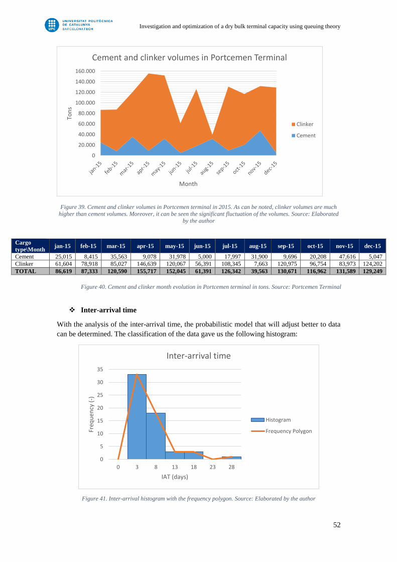
Investigation and optimization of a dry bulk terminal capacity using queuing theory
52
Figure 39. Cement and clinker volumes in Portcemen terminal in 2015. As can be noted, clinker volumes are much
higher than cement volumes. Moreover, it can be seen the significant fluctuation of the volumes. Source: Elaborated
by the author
Inter-arrival time
With the analysis of the inter-arrival time, the probabilistic model that will adjust better to data
can be determined. The classification of the data gave us the following histogram:
Figure 41. Inter-arrival histogram with the frequency polygon. Source: Elaborated by the author
0
20.000
40.000
60.000
80.000
100.000
120.000
140.000
160.000To
ns
Month
Cement and clinker volumes in Portcemen Terminal
Clinker
Cement
0
5
10
15
20
25
30
35
0 3 8 13 18 23 28
Freq
uen
cy (
-)
IAT (days)
Inter-arrival time
Histogram
Frequency Polygon
Cargo
type\Month jan-15 feb-15 mar-15 apr-15 may-15 jun-15 jul-15 aug-15 sep-15 oct-15 nov-15 dec-15
Cement 25,015 8,415 35,563 9,078 31,978 5,000 17,997 31,900 9,696 20,208 47,616 5,047
Clinker 61,604 78,918 85,027 146,639 120,067 56,391 108,345 7,663 120,975 96,754 83,973 124,202
TOTAL 86,619 87,333 120,590 155,717 152,045 61,391 126,342 39,563 130,671 116,962 131,589 129,249
Figure 40. Cement and clinker month evolution in Portcemen terminal in tons. Source: Portcemen Terminal

Investigation and optimization of a dry bulk terminal capacity using queuing theory
53
The table below shows the values calculated to draw the inter-arrival diagram.
Where,
H: Class interval
x: Mean between lower and upper limit
ni: Absolute frequency
fi: Relative frequency (%)
Ni: Cumulative frequency
Fi: Cumulative frequency (%)
Based on these parameters and through the cumulative frequency, the following histogram can be
performed.
Figure 43. Inter-arrival histogram with the cumulative frequency. Source: Elaborated by the author
0%
20%
40%
60%
80%
100%
120%
0
5
10
15
20
25
30
35
0 3 8 13 18 23 28
Freq
uen
cy (
-)
IAT (days)
Inter-arrival time
Histogram
Cumulative Frequency
H Lower limit Upper limit x ni fi Ni Fi
0 0 0 0 0 0% 0 0%
1 1 5 3 33 57% 33 57%
2 6 10 8 18 31% 51 88%
3 11 15 13 3 5% 54 93%
4 16 20 18 3 5% 57 98%
5 21 25 23 0 0% 57 98%
6 26 30 28 1 2% 58 100%
Figure 42. Parameters of inter-arrival histogram. Source: Elaborated by the author
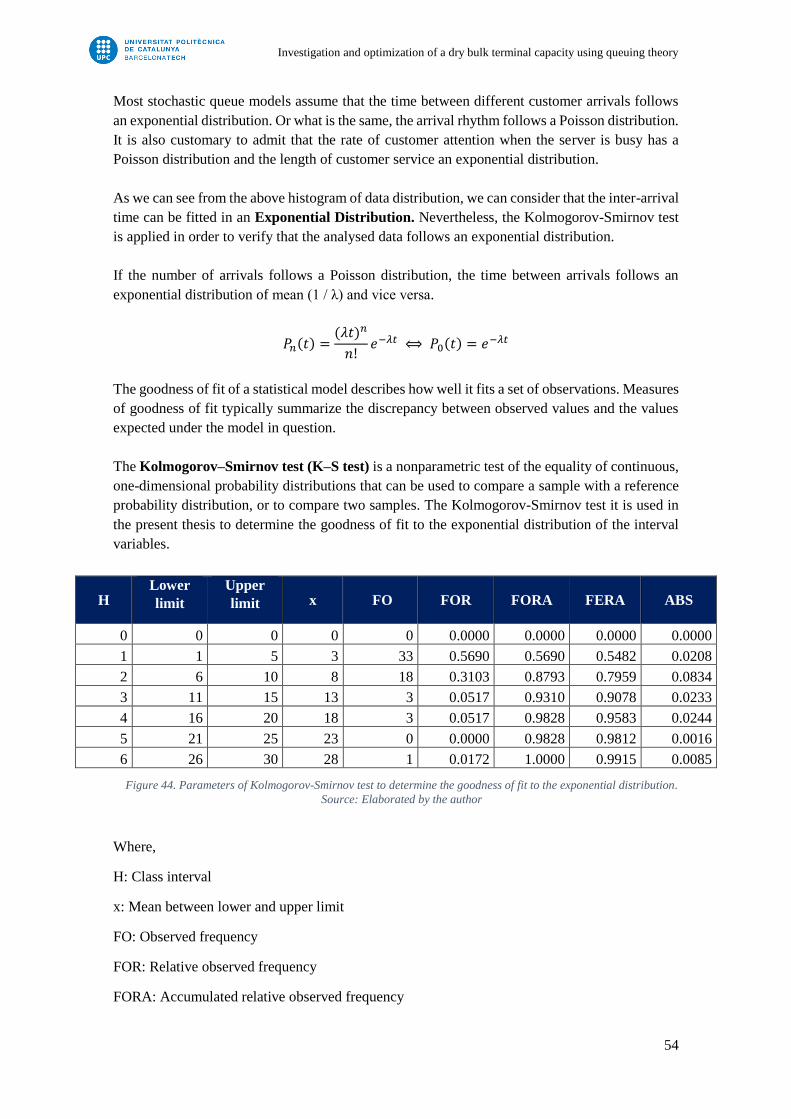
Investigation and optimization of a dry bulk terminal capacity using queuing theory
54
Most stochastic queue models assume that the time between different customer arrivals follows
an exponential distribution. Or what is the same, the arrival rhythm follows a Poisson distribution.
It is also customary to admit that the rate of customer attention when the server is busy has a
Poisson distribution and the length of customer service an exponential distribution.
As we can see from the above histogram of data distribution, we can consider that the inter-arrival
time can be fitted in an Exponential Distribution. Nevertheless, the Kolmogorov-Smirnov test
is applied in order to verify that the analysed data follows an exponential distribution.
If the number of arrivals follows a Poisson distribution, the time between arrivals follows an
exponential distribution of mean (1 / λ) and vice versa.
𝑃𝑛(𝑡) =(𝜆𝑡)𝑛
𝑛!𝑒−𝜆𝑡 ⟺ 𝑃0(𝑡) = 𝑒−𝜆𝑡
The goodness of fit of a statistical model describes how well it fits a set of observations. Measures
of goodness of fit typically summarize the discrepancy between observed values and the values
expected under the model in question.
The Kolmogorov–Smirnov test (K–S test) is a nonparametric test of the equality of continuous,
one-dimensional probability distributions that can be used to compare a sample with a reference
probability distribution, or to compare two samples. The Kolmogorov-Smirnov test it is used in
the present thesis to determine the goodness of fit to the exponential distribution of the interval
variables.
Where,
H: Class interval
x: Mean between lower and upper limit
FO: Observed frequency
FOR: Relative observed frequency
FORA: Accumulated relative observed frequency
H Lower
limit
Upper
limit x FO FOR FORA FERA ABS
0 0 0 0 0 0.0000 0.0000 0.0000 0.0000
1 1 5 3 33 0.5690 0.5690 0.5482 0.0208
2 6 10 8 18 0.3103 0.8793 0.7959 0.0834
3 11 15 13 3 0.0517 0.9310 0.9078 0.0233
4 16 20 18 3 0.0517 0.9828 0.9583 0.0244
5 21 25 23 0 0.0000 0.9828 0.9812 0.0016
6 26 30 28 1 0.0172 1.0000 0.9915 0.0085
Figure 44. Parameters of Kolmogorov-Smirnov test to determine the goodness of fit to the exponential distribution.
Source: Elaborated by the author

Investigation and optimization of a dry bulk terminal capacity using queuing theory
55
FERA: Accumulated relative expected frequency
ABS: Absolute frequency (ABS=FORA-FERA)
Hypothesis to contrast:
H0: The data follow an exponential distribution
H1: The data do not follow an exponential distribution
Test Statistic: The Kolmogorov-Smirnov test statistic is defined as:
𝐷 = sup𝑙≤𝑖≤𝑛
|�̂�𝑛(𝑥𝑖) − 𝐹0(𝑥𝑖)|
Where,
𝑥𝑖 is the i-th value observed in the sample.
�̂�𝑛(𝑥𝑖) is an estimator of the probability of observing values that are less than or equal to 𝑥𝑖.
𝐹0(𝑥𝑖) is the probability of observing values less than or equal to 𝑥𝑖 when H0 is true.
Significance Level: α = 0.05
Therefore, the criteria for making the decision between the 2 hypothesis will be:
𝐼𝑓 𝐷 ≤ 𝐷∝ ⟹ 𝐴𝑐𝑐𝑒𝑝𝑡 𝐻0
𝐼𝑓 𝐷 > 𝐷∝ ⟹ 𝑅𝑒𝑗𝑒𝑐𝑡 𝐻0
Where 𝐷∝ is defined:
𝐷∝ =𝑐∝
𝑘(𝑛)
Where 𝑐∝ and 𝑘(𝑛) are extracted from the table in Annex F.
Figure 45. Table of Kolmogorov-Smirnov test estimator of Goodness of Fit. Marked in red, the calculation of 𝐷∝ for
an n>50 and α=0.05. Source: http://www4.ujaen.es/~mpfrias/TablasInferencia.pdf

Investigation and optimization of a dry bulk terminal capacity using queuing theory
56
With the calculations of D and 𝐷∝ done, the criteria for making the decision between the 2
hypothesis can be applied. The result is the following:
Estimator Smirnov-kolmogorov (D) 0.0834
Degrees of freedom 58
𝐷∝ (α=0.05) 0.1786
Test Accept
There is no contrary statistical evidence to reject the proposed model. Thus, it can be assumed the
data follows an exponential Distribution.
The exponential distribution occurs naturally when describing the lengths of the inter-arrival
times in a homogeneous Poisson process. In queuing theory, the service times of agents in a
system are often modelled as exponentially distributed variables. The arrival of customers for
instance is also modelled by the Poisson distribution if the arrivals are independent and distributed
identically. The length of a process that can be thought of as a sequence of several independent
tasks follows the Erlang distribution (which is the distribution of the sum of several independent
exponentially distributed variables). Reliability theory and reliability engineering also make
extensive use of the exponential distribution. Because of the memoryless property of this
distribution, it is well-suited to model the constant hazard rate portion of the bathtub curve used
in reliability theory.
Vessels arrivals
The mode for ships queuing is the key to establish a fine handling queuing system, making the
operation of handling queuing system smoothly. According to the characteristics of handling in
the ports and ships as well as a great amounts of statistics data and study abroad, it can be shown
that, in most queuing systems for handling service, the arrival of the ships obeys the Poisson
distribution while the time for handling service obeys the negative exponential distribution.
The ships arrivals and service times are totally random so they comply with the pattern of random
occurrences. Moreover, it is assumed that the queue length is unlimited, that is, if a ship arrives
and finds a long queue, it joins the waiting ships and does not leave the port. Vessels are processed
on the “First come, first served” queue discipline.
For customers who arrive and find the queue as a stationary process, the response time they
experience (the sum of both waiting time and service time) follows the probability density
function:
𝑓(𝑥) = {(𝜇 − 𝜆)𝑒−(𝜇−𝜆)𝑡, 𝑡 > 0
0, 𝑜𝑡ℎ𝑒𝑟𝑤𝑖𝑠𝑒
The diagram below shows the arrivals in Portcemen terminal in 2015. As can be seen, the
maximum number of vessels that overlap in the same day is 2. This fact only happens in 4 cases
during this year. All year round, there are 307 days in which no vessels arrived, 54 days that
served 1 vessel and 4 days that overlap 2 vessels in the same day.

Investigation and optimization of a dry bulk terminal capacity using queuing theory
57
Figure 46. Arrivals in Portcemen terminal in 2015. Source: Elaborated by the author
The number of arrivals per month is very small so the sample from which the goodness of fit test
is applied is representative but limited. Nevertheless, the Kolmogorov-Smirnov test is applied in
order to verify that the analysed data follows a Poisson distribution.
The Kolmogorov-Smirnov test it is used in the present thesis to determine the goodness of fit to
the Poisson distribution of the interval variables.
0
1
2
3
0 15 30 45 60 75 90 105120135150165180195210225240255270285300315330345360
Ves
sels
Days
Arrivals in Portcemen terminal in 2015 # Vessels in…
Month Arrivals
1 5
2 3
3 6
4 5
5 5
6 3
7 6
8 4
9 6
10 5
11 6
12 4
Figure 48. Number of arrivals per month in
Portcemen Terminal in 2015. Source:
Elaborated by the author.
H Lower
limit
Upper
limit x FO FOR FORA FERA ABS
0 0 0 0 0 0.0000 0.0000 0.0000 0.0000
1 3 3 3 2 0.1667 0.1667 0.2892 -0.1225
2 4 4 4 2 0.1667 0.3333 0.4702 -0.1369
3 5 5 5 4 0.3333 0.6667 0.6452 0.0215
4 6 6 6 5 0.3333 1.0000 0.7861 0.2139
Figure 49. Parameters of Kolmogorov-Smirnov test to determine the goodness of fit to the Poisson distribution.
Source: Elaborated by the author
Figure 47. Ships arrival distribution as Poisson function,
hypothetical port. Source: El-Naggar, M. E., Application of
queuing theory to the container terminal at Alexandria seaport.

Investigation and optimization of a dry bulk terminal capacity using queuing theory
58
Where,
H: Class interval
x: Mean between lower and upper limit
FO: Observed frequency
FOR: Relative observed frequency
FORA: Accumulated relative observed frequency
FERA: Accumulated relative expected frequency
ABS: Absolute frequency (ABS=FORA-FERA)
Hypothesis to contrast:
H0: The data follow a Poisson distribution
H1: The data do not follow a Poisson distribution
Test Statistic: The Kolmogorov-Smirnov test statistic is defined as:
𝐷 = sup𝑙≤𝑖≤𝑛
|�̂�𝑛(𝑥𝑖) − 𝐹0(𝑥𝑖)|
Where,
𝑥𝑖 is the i-th value observed in the sample.
�̂�𝑛(𝑥𝑖) is an estimator of the probability of observing values that are less than or equal to 𝑥𝑖.
𝐹0(𝑥𝑖) is the probability of observing values less than or equal to 𝑥𝑖 when H0 is true.
Significance Level: α = 0.05
Therefore, the criteria for making the decision between the 2 hypothesis will be:
𝐼𝑓 𝐷 ≤ 𝐷∝ ⟹ 𝐴𝑐𝑐𝑒𝑝𝑡 𝐻0
𝐼𝑓 𝐷 > 𝐷∝ ⟹ 𝑅𝑒𝑗𝑒𝑐𝑡 𝐻0
Where 𝐷∝ is defined:
𝐷∝ =𝑐∝
𝑘(𝑛)
Where 𝑐∝ and 𝑘(𝑛), where n=12, are extracted from the table in Annex F.
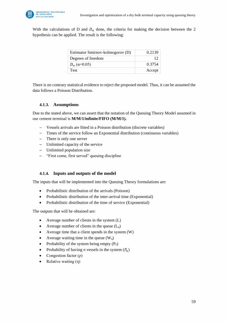
Investigation and optimization of a dry bulk terminal capacity using queuing theory
59
With the calculations of D and 𝐷∝ done, the criteria for making the decision between the 2
hypothesis can be applied. The result is the following:
Estimator Smirnov-kolmogorov (D) 0.2139
Degrees of freedom 12
𝐷∝ (α=0.05) 0.3754
Test Accept
There is no contrary statistical evidence to reject the proposed model. Thus, it can be assumed the
data follows a Poisson Distribution.
4.1.3. Assumptions
Due to the stated above, we can assert that the notation of the Queuing Theory Model assumed in
our cement terminal is M/M/1/infinite/FIFO (M/M/1).
─ Vessels arrivals are fitted in a Poisson distribution (discrete variables)
─ Times of the service follow an Exponential distribution (continuous variables)
─ There is only one server
─ Unlimited capacity of the service
─ Unlimited population size
─ “First come, first served” queuing discipline
4.1.4. Inputs and outputs of the model
The inputs that will be implemented into the Queuing Theory formulations are:
Probabilistic distribution of the arrivals (Poisson)
Probabilistic distribution of the inter-arrival time (Exponential)
Probabilistic distribution of the time of service (Exponential)
The outputs that will be obtained are:
Average number of clients in the system (L)
Average number of clients in the queue (Lq)
Average time that a client spends in the system (W)
Average waiting time in the queue (Wq)
Probability of the system being empty (P0)
Probability of having n vessels in the system (𝑃𝑛)
Congestion factor (ρ)
Relative waiting (η)
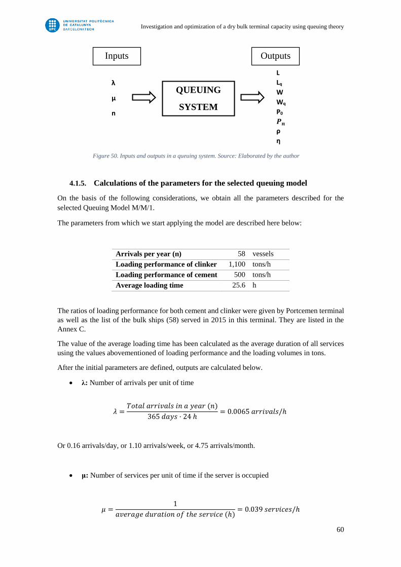
Investigation and optimization of a dry bulk terminal capacity using queuing theory
60
4.1.5. Calculations of the parameters for the selected queuing model
On the basis of the following considerations, we obtain all the parameters described for the
selected Queuing Model M/M/1.
The parameters from which we start applying the model are described here below:
Arrivals per year (n) 58 vessels
Loading performance of clinker 1,100 tons/h
Loading performance of cement 500 tons/h
Average loading time 25.6 h
The ratios of loading performance for both cement and clinker were given by Portcemen terminal
as well as the list of the bulk ships (58) served in 2015 in this terminal. They are listed in the
Annex C.
The value of the average loading time has been calculated as the average duration of all services
using the values abovementioned of loading performance and the loading volumes in tons.
After the initial parameters are defined, outputs are calculated below.
λ: Number of arrivals per unit of time
𝜆 =𝑇𝑜𝑡𝑎𝑙 𝑎𝑟𝑟𝑖𝑣𝑎𝑙𝑠 𝑖𝑛 𝑎 𝑦𝑒𝑎𝑟 (𝑛)
365 𝑑𝑎𝑦𝑠 · 24 ℎ= 0.0065 𝑎𝑟𝑟𝑖𝑣𝑎𝑙𝑠/ℎ
Or 0.16 arrivals/day, or 1.10 arrivals/week, or 4.75 arrivals/month.
μ: Number of services per unit of time if the server is occupied
𝜇 =1
𝑎𝑣𝑒𝑟𝑎𝑔𝑒 𝑑𝑢𝑟𝑎𝑡𝑖𝑜𝑛 𝑜𝑓 𝑡ℎ𝑒 𝑠𝑒𝑟𝑣𝑖𝑐𝑒 (ℎ)= 0.039 𝑠𝑒𝑟𝑣𝑖𝑐𝑒𝑠/ℎ
λ
μ
n
L
Lq
W
Wq
P0
𝑷𝒏
ρ
η
QUEUING
SYSTEM
Inputs Outputs
Figure 50. Inputs and outputs in a queuing system. Source: Elaborated by the author

Investigation and optimization of a dry bulk terminal capacity using queuing theory
61
Or 0.938 services/day.
Where the average duration of the service is 25.6 hours.
ρ: Congestion factor
𝜌 =𝜆
𝜇= 0.167
Where λ<< μ.
P0: Probability of the system being empty
𝑃0 = 1 − 𝜌 = 0,833 = 83%
𝑷𝒏: Probability of having n vessels in the system
𝑃𝑛 = (1 − 𝜌) · 𝜌𝑛
In case of n=1, 𝑃1 = 13.88%
In case of n=2, 𝑃2 = 2.312%
L: Average number of clients in the system
𝐿 =𝜌
1 − 𝜌=
𝜆
𝜇 − 𝜆= 0.1998 𝑣𝑒𝑠𝑠𝑒𝑙𝑠
Lq: Average number of clients in the queue
𝐿𝑞 =𝜆2
𝜇 · (𝜇 − 𝜆)=
𝜌2
1 − 𝜌= 0.033 𝑣𝑒𝑠𝑠𝑒𝑙𝑠
W: Average time that a client spends in the system
𝑊 =𝐿
𝜆=
1
𝜇 − 𝜆= 30.717 ℎ
Wq: Average waiting time in the queue
𝑊𝑞 =𝜌
𝜇 − 𝜆= 5.117 ℎ
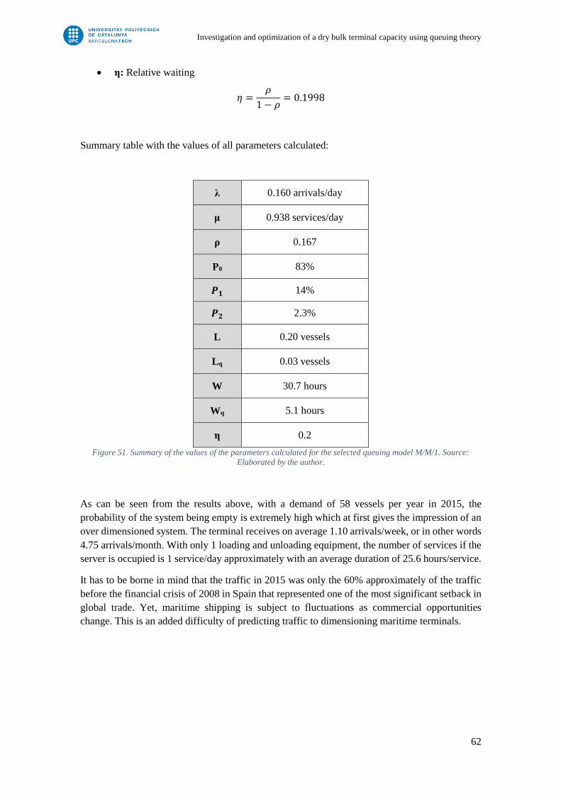
Investigation and optimization of a dry bulk terminal capacity using queuing theory
62
η: Relative waiting
𝜂 =𝜌
1 − 𝜌= 0.1998
Summary table with the values of all parameters calculated:
λ 0.160 arrivals/day
μ 0.938 services/day
ρ 0.167
P0 83%
𝑷𝟏 14%
𝑷𝟐 2.3%
L 0.20 vessels
Lq 0.03 vessels
W 30.7 hours
Wq 5.1 hours
η 0.2
Figure 51. Summary of the values of the parameters calculated for the selected queuing model M/M/1. Source:
Elaborated by the author.
As can be seen from the results above, with a demand of 58 vessels per year in 2015, the
probability of the system being empty is extremely high which at first gives the impression of an
over dimensioned system. The terminal receives on average 1.10 arrivals/week, or in other words
4.75 arrivals/month. With only 1 loading and unloading equipment, the number of services if the
server is occupied is 1 service/day approximately with an average duration of 25.6 hours/service.
It has to be borne in mind that the traffic in 2015 was only the 60% approximately of the traffic
before the financial crisis of 2008 in Spain that represented one of the most significant setback in
global trade. Yet, maritime shipping is subject to fluctuations as commercial opportunities
change. This is an added difficulty of predicting traffic to dimensioning maritime terminals.
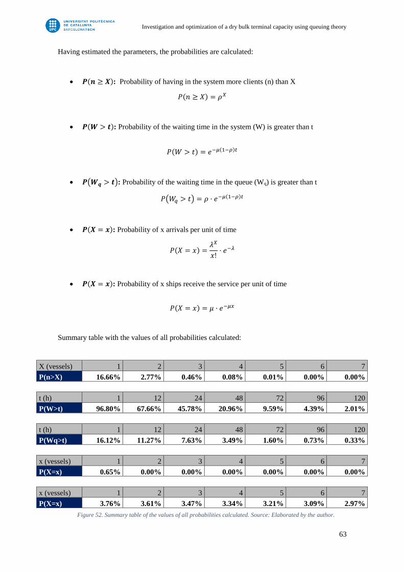
Investigation and optimization of a dry bulk terminal capacity using queuing theory
63
Having estimated the parameters, the probabilities are calculated:
𝑷(𝒏 ≥ 𝑿): Probability of having in the system more clients (n) than X
𝑃(𝑛 ≥ 𝑋) = 𝜌𝑋
𝑷(𝑾 > 𝒕): Probability of the waiting time in the system (W) is greater than t
𝑃(𝑊 > 𝑡) = 𝑒−𝜇(1−𝜌)𝑡
𝑷(𝑾𝒒 > 𝒕): Probability of the waiting time in the queue (Wq) is greater than t
𝑃(𝑊𝑞 > 𝑡) = 𝜌 · 𝑒−𝜇(1−𝜌)𝑡
𝑷(𝑿 = 𝒙): Probability of x arrivals per unit of time
𝑃(𝑋 = 𝑥) =𝜆𝑋
𝑥!· 𝑒−𝜆
𝑷(𝑿 = 𝒙): Probability of x ships receive the service per unit of time
𝑃(𝑋 = 𝑥) = 𝜇 · 𝑒−𝜇𝑥
Summary table with the values of all probabilities calculated:
X (vessels) 1 2 3 4 5 6 7
P(n>X) 16.66% 2.77% 0.46% 0.08% 0.01% 0.00% 0.00%
t (h) 1 12 24 48 72 96 120
P(W>t) 96.80% 67.66% 45.78% 20.96% 9.59% 4.39% 2.01%
t (h) 1 12 24 48 72 96 120
P(Wq>t) 16.12% 11.27% 7.63% 3.49% 1.60% 0.73% 0.33%
x (vessels) 1 2 3 4 5 6 7
P(X=x) 0.65% 0.00% 0.00% 0.00% 0.00% 0.00% 0.00%
x (vessels) 1 2 3 4 5 6 7
P(X=x) 3.76% 3.61% 3.47% 3.34% 3.21% 3.09% 2.97%
Figure 52. Summary table of the values of all probabilities calculated. Source: Elaborated by the author.
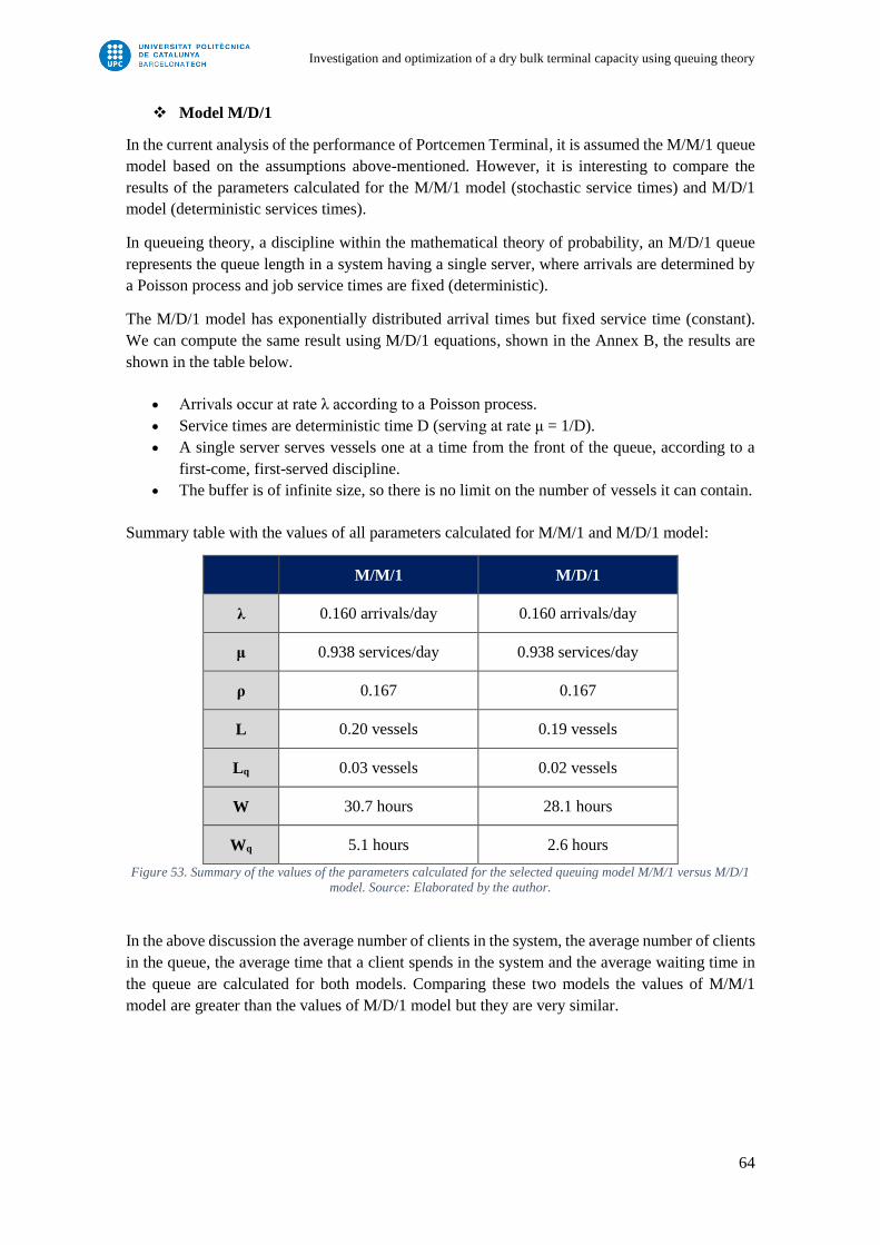
Investigation and optimization of a dry bulk terminal capacity using queuing theory
64
Model M/D/1
In the current analysis of the performance of Portcemen Terminal, it is assumed the M/M/1 queue
model based on the assumptions above-mentioned. However, it is interesting to compare the
results of the parameters calculated for the M/M/1 model (stochastic service times) and M/D/1
model (deterministic services times).
In queueing theory, a discipline within the mathematical theory of probability, an M/D/1 queue
represents the queue length in a system having a single server, where arrivals are determined by
a Poisson process and job service times are fixed (deterministic).
The M/D/1 model has exponentially distributed arrival times but fixed service time (constant).
We can compute the same result using M/D/1 equations, shown in the Annex B, the results are
shown in the table below.
Arrivals occur at rate λ according to a Poisson process.
Service times are deterministic time D (serving at rate μ = 1/D).
A single server serves vessels one at a time from the front of the queue, according to a
first-come, first-served discipline.
The buffer is of infinite size, so there is no limit on the number of vessels it can contain.
Summary table with the values of all parameters calculated for M/M/1 and M/D/1 model:
M/M/1 M/D/1
λ 0.160 arrivals/day 0.160 arrivals/day
μ 0.938 services/day 0.938 services/day
ρ 0.167 0.167
L 0.20 vessels 0.19 vessels
Lq 0.03 vessels 0.02 vessels
W 30.7 hours 28.1 hours
Wq 5.1 hours 2.6 hours
Figure 53. Summary of the values of the parameters calculated for the selected queuing model M/M/1 versus M/D/1
model. Source: Elaborated by the author.
In the above discussion the average number of clients in the system, the average number of clients
in the queue, the average time that a client spends in the system and the average waiting time in
the queue are calculated for both models. Comparing these two models the values of M/M/1
model are greater than the values of M/D/1 model but they are very similar.

Investigation and optimization of a dry bulk terminal capacity using queuing theory
65
4.1.6. Simulation
Although the larger vessels have real scheduled arrivals, the smaller ones do not. It is necessary
to assume the random nature of the arrivals in case of non-programmed calls.
It should also be considered that the duration of the calls is not fixed, but dependent on the amount
of cement and clinker to be loaded. Moreover, the crane performance sets the duration of the
service. Departures are also considered random due to their dependency on the volume of
commodities loaded and unloaded.
For this reason, a temporal analysis of the traffic patterns is developed on Portcemen terminal so
as to simulate the dynamics of the terminal and determine feasible scenarios.
This analysis evaluates how many vessels are berthed at Portcemen terminal in year 2015,
considered as the result of evaluating the total arrivals and the total time of the service which
comes from the ship loader’s performance for both cement and clinker.
Loading performance of clinker 1,100 tons/h
Loading performance of cement 500 tons/h
Due to the data provided was complete but not sufficient enough, for developing the simulation,
they are assumed the following scenarios:
Ship loaders work 24 hours/day
No preparation time for the machines is considered
All vessels arrive at 8:00 am
Once the sequence of arrivals is sorted out with their corresponding cargo and the volume of tons
which have to be loaded, applying the loading performance of cement and clinker, the loading
time for each service can be determined, and so the service time. The average loading time is 25.6
hours per service, in other words, 1 day per service approximately.
As it is mentioned above, every service lasts 25.6 hours in average, meaning that the server is
working 17% of the time in a year.
With the arrival times and the service times determined, the simulation can proceed in order to
acquire the departure times. Thus, it can be seen how many vessels might wait in queue for the
service.
In the following table, all the values abovementioned for each call in Portcemen are shown. The
results of the analysis reveal that in 4 different occasions during the year, vessels have to wait to
be served. The average waiting time of these 4 vessels is 15 hours.
In order to preserve the data confidentiality, the detailed information of the arrivals such as cargo
(cement or clinker) and Tm have not been shown in the table below.
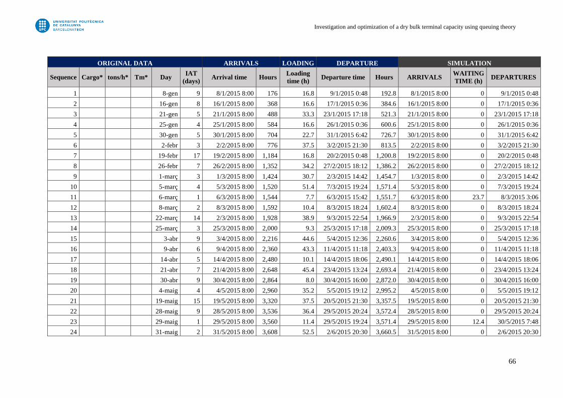
Investigation and optimization of a dry bulk terminal capacity using queuing theory
66
ORIGINAL DATA ARRIVALS LOADING DEPARTURE SIMULATION
Sequence Cargo* tons/h* Tm* Day IAT
(days) Arrival time Hours
Loading
time (h) Departure time Hours ARRIVALS
WAITING
TIME (h) DEPARTURES
1 8-gen 9 8/1/2015 8:00 176 16.8 9/1/2015 0:48 192.8 8/1/2015 8:00 0 9/1/2015 0:48
2 16-gen 8 16/1/2015 8:00 368 16.6 17/1/2015 0:36 384.6 16/1/2015 8:00 0 17/1/2015 0:36
3 21-gen 5 21/1/2015 8:00 488 33.3 23/1/2015 17:18 521.3 21/1/2015 8:00 0 23/1/2015 17:18
4 25-gen 4 25/1/2015 8:00 584 16.6 26/1/2015 0:36 600.6 25/1/2015 8:00 0 26/1/2015 0:36
5 30-gen 5 30/1/2015 8:00 704 22.7 31/1/2015 6:42 726.7 30/1/2015 8:00 0 31/1/2015 6:42
6 2-febr 3 2/2/2015 8:00 776 37.5 3/2/2015 21:30 813.5 2/2/2015 8:00 0 3/2/2015 21:30
7 19-febr 17 19/2/2015 8:00 1,184 16.8 20/2/2015 0:48 1,200.8 19/2/2015 8:00 0 20/2/2015 0:48
8 26-febr 7 26/2/2015 8:00 1,352 34.2 27/2/2015 18:12 1,386.2 26/2/2015 8:00 0 27/2/2015 18:12
9 1-març 3 1/3/2015 8:00 1,424 30.7 2/3/2015 14:42 1,454.7 1/3/2015 8:00 0 2/3/2015 14:42
10 5-març 4 5/3/2015 8:00 1,520 51.4 7/3/2015 19:24 1,571.4 5/3/2015 8:00 0 7/3/2015 19:24
11 6-març 1 6/3/2015 8:00 1,544 7.7 6/3/2015 15:42 1,551.7 6/3/2015 8:00 23.7 8/3/2015 3:06
12 8-març 2 8/3/2015 8:00 1,592 10.4 8/3/2015 18:24 1,602.4 8/3/2015 8:00 0 8/3/2015 18:24
13 22-març 14 2/3/2015 8:00 1,928 38.9 9/3/2015 22:54 1,966.9 2/3/2015 8:00 0 9/3/2015 22:54
14 25-març 3 25/3/2015 8:00 2,000 9.3 25/3/2015 17:18 2,009.3 25/3/2015 8:00 0 25/3/2015 17:18
15 3-abr 9 3/4/2015 8:00 2,216 44.6 5/4/2015 12:36 2,260.6 3/4/2015 8:00 0 5/4/2015 12:36
16 9-abr 6 9/4/2015 8:00 2,360 43.3 11/4/2015 11:18 2,403.3 9/4/2015 8:00 0 11/4/2015 11:18
17 14-abr 5 14/4/2015 8:00 2,480 10.1 14/4/2015 18:06 2,490.1 14/4/2015 8:00 0 14/4/2015 18:06
18 21-abr 7 21/4/2015 8:00 2,648 45.4 23/4/2015 13:24 2,693.4 21/4/2015 8:00 0 23/4/2015 13:24
19 30-abr 9 30/4/2015 8:00 2,864 8.0 30/4/2015 16:00 2,872.0 30/4/2015 8:00 0 30/4/2015 16:00
20 4-maig 4 4/5/2015 8:00 2,960 35.2 5/5/2015 19:12 2,995.2 4/5/2015 8:00 0 5/5/2015 19:12
21 19-maig 15 19/5/2015 8:00 3,320 37.5 20/5/2015 21:30 3,357.5 19/5/2015 8:00 0 20/5/2015 21:30
22 28-maig 9 28/5/2015 8:00 3,536 36.4 29/5/2015 20:24 3,572.4 28/5/2015 8:00 0 29/5/2015 20:24
23 29-maig 1 29/5/2015 8:00 3,560 11.4 29/5/2015 19:24 3,571.4 29/5/2015 8:00 12.4 30/5/2015 7:48
24 31-maig 2 31/5/2015 8:00 3,608 52.5 2/6/2015 20:30 3,660.5 31/5/2015 8:00 0 2/6/2015 20:30

Investigation and optimization of a dry bulk terminal capacity using queuing theory
67
25 8-juny 8 8/6/2015 8:00 3,800 44.2 10/6/2015 12:12 3,844.2 8/6/2015 8:00 0 10/6/2015 12:12
26 11-juny 3 11/6/2015 8:00 3,872 10.0 11/6/2015 18:00 3,882.0 11/6/2015 8:00 0 11/6/2015 18:00
27 12-juny 1 12/6/2015 8:00 3,896 7.1 12/6/2015 15:06 3,903.1 12/6/2015 8:00 0 12/6/2015 15:06
28 1-jul 19 1/7/2015 8:00 4,352 9.2 1/7/2015 17:12 4,361.2 1/7/2015 8:00 0 1/7/2015 17:12
29 7-jul 6 7/7/2015 8:00 4,496 18.2 8/7/2015 2:12 4,514.2 7/7/2015 8:00 0 8/7/2015 2:12
30 10-jul 3 10/7/2015 8:00 4,568 43.5 12/7/2015 11:30 4,611.5 10/7/2015 8:00 0 12/7/2015 11:30
31 12-jul 2 12/7/2015 8:00 4,616 10.1 12/7/2015 18:06 4,626.1 12/7/2015 8:00 0 12/7/2015 18:06
32 22-jul 10 22/7/2015 8:00 4,856 36.9 23/7/2015 20:54 4,892.9 22/7/2015 8:00 0 23/7/2015 20:54
33 27-jul 5 27/7/2015 8:00 4,976 16.6 8/7/2015 0:36 4,992.6 27/7/2015 8:00 0 8/7/2015 0:36
34 6-ag 10 6/8/2015 8:00 5,216 8.3 6/8/2015 16:18 5,224.3 6/8/2015 8:00 0 6/8/2015 16:18
35 19-ag 13 19/8/2015 8:00 5,528 9.1 19/8/2015 17:06 5,537.1 19/8/2015 8:00 0 19/8/2015 17:06
36 22-ag 3 22/8/2015 8:00 5,600 46.4 24/8/2015 14:24 5,646.4 22/8/2015 8:00 0 24/8/2015 14:24
37 29-ag 7 29/8/2015 8:00 5,768 7.0 29/8/2015 15:00 5,775.0 29/8/2015 8:00 0 29/8/2015 15:00
38 1-set 3 1/9/2015 8:00 5,840 24.8 10/9/2015 8:48 5,864.8 1/9/2015 8:00 0 10/9/2015 8:48
39 5-set 4 5/9/2015 8:00 5,936 9.3 5/9/2015 17:18 5,945.3 5/9/2015 8:00 0 5/9/2015 17:18
40 9-set 4 9/9/2015 8:00 6,032 33.5 10/9/2015 17:30 6,065.5 9/9/2015 8:00 0 10/9/2015 17:30
41 13-set 4 13/9/2015 8:00 6,128 10.1 13/9/2015 18:06 6,138.1 13/9/2015 8:00 0 13/9/2015 18:06
42 17-set 4 17/9/2015 8:00 6,224 7.1 17/9/2015 15:06 6,231.1 17/9/2015 8:00 0 17/9/2015 15:06
43 24-set 7 24/9/2015 8:00 6,392 44.6 26/9/2015 12:36 6,436.6 24/9/2015 8:00 0 26/9/2015 12:36
44 3-oct 9 3/10/2015 8:00 6,608 37.1 4/10/2015 21:06 6,645.1 3/10/2015 8:00 0 4/10/2015 21:06
45 9-oct 6 9/10/2015 8:00 6,752 10.3 9/10/2015 18:18 6,762.3 9/10/2015 8:00 0 9/10/2015 18:18
46 12-oct 3 12/10/2015 8:00 6,824 43.3 14/10/2015 11:18 6,867.3 12/10/2015 8:00 0 14/10/2015 11:18
47 13-oct 1 13/10/2015 8:00 6,848 30.1 14/10/2015 14:06 6,878.1 13/10/2015 8:00 15.3 15/10/2015 16:54
48 17-oct 4 17/10/2015 8:00 6,944 7.6 17/10/2015 15:36 6,951.6 17/10/2015 8:00 0 17/10/2015 15:36
49 12-nov 26 12/11/2015 8:00 7,568 55.0 14/11/2015 23:00 7,623.0 12/11/2015 8:00 0 14/11/2015 23:00
50 15-nov 3 15/11/2015 8:00 7,640 33.0 16/11/2015 17:00 7,673.0 15/11/2015 8:00 0 16/11/2015 17:00
51 19-nov 4 19/11/2015 8:00 7,736 10.1 19/11/2015 18:06 7,746.1 19/11/2015 8:00 0 19/11/2015 18:06
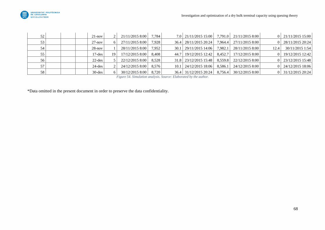
Investigation and optimization of a dry bulk terminal capacity using queuing theory
68
52 21-nov 2 21/11/2015 8:00 7,784 7.0 21/11/2015 15:00 7,791.0 21/11/2015 8:00 0 21/11/2015 15:00
53 27-nov 6 27/11/2015 8:00 7,928 36.4 28/11/2015 20:24 7,964.4 27/11/2015 8:00 0 28/11/2015 20:24
54 28-nov 1 28/11/2015 8:00 7,952 30.1 29/11/2015 14:06 7,982.1 28/11/2015 8:00 12.4 30/11/2015 1:54
55 17-des 19 17/12/2015 8:00 8,408 44.7 19/12/2015 12:42 8,452.7 17/12/2015 8:00 0 19/12/2015 12:42
56 22-des 5 22/12/2015 8:00 8,528 31.8 23/12/2015 15:48 8,559.8 22/12/2015 8:00 0 23/12/2015 15:48
57 24-des 2 24/12/2015 8:00 8,576 10.1 24/12/2015 18:06 8,586.1 24/12/2015 8:00 0 24/12/2015 18:06
58 30-des 6 30/12/2015 8:00 8,720 36.4 31/12/2015 20:24 8,756.4 30/12/2015 8:00 0 31/12/2015 20:24 Figure 54. Simulation analysis. Source: Elaborated by the author.
*Data omitted in the present document in order to preserve the data confidentiality.

Investigation and optimization of a dry bulk terminal capacity using queuing theory
69
The results of the analysis are summarized in the table below.
Average service time (h) 25.6
% of time the server is working 17%
% of time the server is empty 83%
Minimum service time (h) 7
Maximum service time (h) 55
Minimum number of vessels in terminal 0
Number of days a year when the terminal is empty 307
% of the total 84%
Maximum number of vessels in terminal 2
Number of days a year when the maximum number is produced 4
% of the total 1%
Number of days a year when a vessel is at terminal 54
% of the total 15%
Total waiting time of vessels in queue (h) 64
Average waiting time of vessels in queue (h) 15
Minimum inter-arrival time (days) 1
Maximum inter-arrival time (days) 26
Figure 55. Summary of the values calculated. Source: Elaborated by the author.
These ideas improve the knowledge about the behaviour of the traffic patterns at the terminal, and
they will bolster the conclusions obtained from the queuing theory method results.
4.1.7. Levels of service
Terminal capacity calculations provide a link between the level of service achieved and the
following factors: the demand placed, the capacity provided and the performance expected.
When planning facilities, it is necessary to try out different capacities with different traffic
forecasts for different points of time. This calculation will be used for setting performance
(productivity), proposed capacity (number of berths) and varying traffic demand to determine the
effect on level of service (ship waiting time). Alternatively, for a proposed waiting time, traffic
and number of berths for the required productivity can be determined.
All these calculations use liner equations except the ship waiting parameter or queuing times for
berths. As it is previously mentioned in the queuing theory chapter, it is a complex mathematical
expression which for different assumptions may not have a numerical solution. The use of
theoretical queuing formulas and computer simulation models have been used to estimate ship
waiting time. Results from queuing theory are dependent on the statistical distribution of ship
arrivals and ship servicing time.

Investigation and optimization of a dry bulk terminal capacity using queuing theory
70
Charts
For the above reasons, the use of planning charts12 is recommended first to obtain a general vision
and a clear understanding of the relationships and their sensitives, and then as a crosscheck on
calculations. The charts are graphical statements of the linear equations but for greater precision
is preferable to use equations. The relationship between berth utilization and ship waiting time is
plotted by a curve based on queuing theory in the charts. As it is referenced in UNCTAD Manual
“Port development”, the charts only apply for dry bulk terminals.
Hereunder, both charts are shown. The first one, related to berth time, gives the following
information to the planner: effective capacity of each ship-loader or unloader; through-ship gross
loading or unloading rate: through-ship net loading or unloading rate (which is equivalent to the
gross rate if the berth is worked 24 hours per day); and average berth time for individual ships.
The through-ship net rate is a key figure in describing the productivity of a bulk berth.
The planning chart II, related to ship cost, is a similar method as planning chart I with the
following turning points: number of ships per year; number of terminal commission days per year;
number of berths; and the average daily ship cost while at port. The number of terminal
commission days per year is the sum of the number of commission days for each berth. For each
set of turning-points, the intersections of the trajectory and the axes give the planner the following
information: annual berth-day requirement; berth utilization; ship time at port; and annual ship
cost while at port.
Both charts are shown in Annex E of the present thesis.
Waiting time/Service time ratio
According to Spanish Recommendations on Maritime Works (ROM 2.0-11), the service quality
level (𝜏) is defined as relative waiting or average waiting time of ships in port before being
assigned a berth due to the occupancy of all berths divided by the average total time of the vessels
moored at the berth or time of service.
This ratio is widely used as a measure of the level of service provided by a terminal, as would
seem logical, for ships that have less cargo to discharge cannot afford to wait as long as ships that
have more.
Therefore, 𝜏 is the ratio between the waiting time at the queue and the services per unit time that the
terminal provides:
𝜏 =𝑊𝑞
1𝜇⁄
Or, in other words: τ is the proportion of the service time that a vessel has to wait before being
attended:
12 Information extracted from Port development: A handbook for planners in developing countries prepared
by the secretariat of UNCTAD in 1985. Completely referred in the Bibliography.

Investigation and optimization of a dry bulk terminal capacity using queuing theory
71
𝑊𝑞(ℎ) = 𝜏 ·1
𝜇
Regarding the waiting time ratio, the Port Management Manual developed by UNCTAD in 1985
establishes that “It is usually considered that waiting time should be not more than lo-50 per cent
of working time. But this ratio is also misleading since it can improve (i.e. decrease) as service
time deteriorates (i.e. increases). As with berth occupancy, the ratio should be used only when
the other factors are constant. When the plan has been based on investing for the economic
optimum, the waiting-time/service-time ratio is bound to be an acceptable figure, generally less
than 30 per cent.”
For this minor thesis, the performance of the terminal will be evaluated considering the average
waiting time in queue (Wq) and service time (μ) that have been defined previously and
characterized analytically in section 4.1.5 in the calculations of the parameters for the selected
queuing model.
On the other hand, regarding the “Recommendations for the project and execution of docking and
mooring works” by the Spanish Recommendations on Maritime Works (ROM 2.0-11), it
establishes that “In general, relatives waiting times between 0.1 and 0.5 are considered
admissible depending on the characteristics of the fleet expected at berthing. That is, average
waiting times between 10% (for totally regular traffic) and 50% (for totally tramp traffic) of the
average service time, with intermediate values for mixed traffic.”
According to the explained above, the value of the ratio (𝜏) will be obtained of the simulation
scenarios previously defined. Once this value is obtained, it will be compared with the criteria of
admissible waiting time defined by UNCTAD and with the one defined by ROM. The fulfilment
or unfulfilment of these criteria will conform the core of the assessment of the Portcemen terminal
performance in which is based this minor thesis.
Summarizing, the criteria evaluated are the following:
From UNTAD: Admissible waiting time less than 30% (admissible 𝜏 less than 0.3)
From ROM: Admissible 𝜏 between 0.1 and 0.5
Investigation and optimization of a dry bulk terminal capacity using queuing theory
72
4.2.Future situation
In normal circumstances, improving service levels and increasing the number of servers, can
improve the service efficiency and reduce the waiting time. However, improving the level of
service and increasing the number of servers will increase the service costs too. Therefore, to
achieve the purpose of optimization, we must make the sum of service cost and waiting cost to be
minimal.
Previously, the parameters for the queuing model applied in our case of study (M/M/1) in
Portcemen terminal during 2015 have been calculated. A study of resilience has been carried out
to analyze eventual scenarios that may occur in the future. For this, the parameters for other
selected model have been calculated.
The proposed scenarios that have been analyzed are:
Increasing the demand
Increasing the servers
Aside from modifying the real data of 2015 by varying the demand and the servers, the rest of the
parameters contemplated in the data of Portcemen terminal will be sustained such as the ship
loaders performance or the average loading time.
Once these 2 situations outlined above are staged, they will be compared with the criteria of
admissible waiting time defined by UNCTAD and with the one defined by ROM.
The criteria evaluated are the following:
From UNTAD: Admissible waiting time less than 30% (admissible 𝜏 less than 0.3)
From ROM: Admissible 𝜏 between 0.1 and 0.5
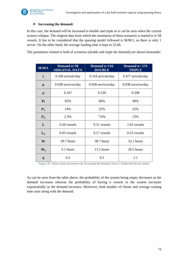
Investigation and optimization of a dry bulk terminal capacity using queuing theory
73
Increasing the demand:
In this case, the demand will be increased to double and triple so it can be seen when the current
system collapse. The original data from which the simulation of these scenarios is started is n=58
vessels. It has to be considered that the queuing model followed is M/M/1, so there is only 1
server. On the other hand, the average loading time is kept in 25.6h.
The parameters related to both of scenarios (double and triple the demand) are shown hereunder.
M/M/1 Demand n=58
ORIGINAL DATA
Demand n=116
DOUBLE
Demand n= 174
TRIPLE
λ 0.160 arrivals/day 0.318 arrivals/day 0.477 arrivals/day
μ 0.938 services/day 0.938 services/day 0.938 services/day
ρ 0.167 0.339 0.508
P0 83% 66% 49%
𝑷𝟏 14% 22% 25%
𝑷𝟐 2.3% 7.6% 13%
L 0.20 vessels 0.51 vessels 1.03 vessels
Lq 0.03 vessels 0.17 vessels 0.53 vessels
W 30.7 hours 38.7 hours 52.1 hours
Wq 5.1 hours 13.1 hours 26.5 hours
η 0.2 0.5 1.1
Figure 56. Values of the parameters by increasing the demand. Source: Elaborated by the author
As can be seen from the table above, the probability of the system being empty decreases as the
demand increases whereas the probability of having n vessels in the system increases
exponentially as the demand increases. Moreover, both number of clients and average waiting
time raise along with the demand.
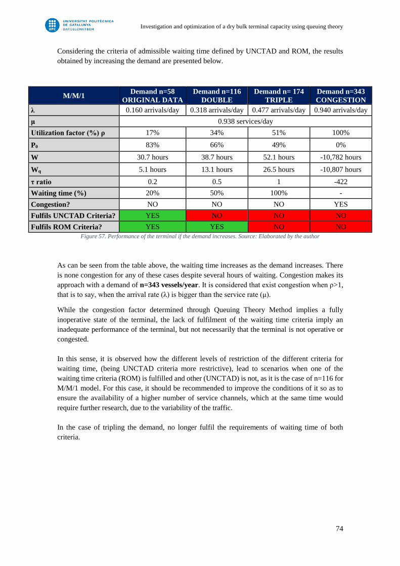
Investigation and optimization of a dry bulk terminal capacity using queuing theory
74
Considering the criteria of admissible waiting time defined by UNCTAD and ROM, the results
obtained by increasing the demand are presented below.
M/M/1 Demand n=58
ORIGINAL DATA
Demand n=116
DOUBLE
Demand n= 174
TRIPLE
Demand n=343
CONGESTION
λ 0.160 arrivals/day 0.318 arrivals/day 0.477 arrivals/day 0.940 arrivals/day
μ 0.938 services/day
Utilization factor (%) ρ 17% 34% 51% 100%
P0 83% 66% 49% 0%
W 30.7 hours 38.7 hours 52.1 hours -10,782 hours
Wq 5.1 hours 13.1 hours 26.5 hours -10,807 hours
τ ratio 0.2 0.5 1 -422
Waiting time (%) 20% 50% 100% -
Congestion? NO NO NO YES
Fulfils UNCTAD Criteria? YES NO NO NO
Fulfils ROM Criteria? YES YES NO NO
Figure 57. Performance of the terminal if the demand increases. Source: Elaborated by the author
As can be seen from the table above, the waiting time increases as the demand increases. There
is none congestion for any of these cases despite several hours of waiting. Congestion makes its
approach with a demand of n=343 vessels/year. It is considered that exist congestion when ρ>1,
that is to say, when the arrival rate (λ) is bigger than the service rate (μ).
While the congestion factor determined through Queuing Theory Method implies a fully
inoperative state of the terminal, the lack of fulfilment of the waiting time criteria imply an
inadequate performance of the terminal, but not necessarily that the terminal is not operative or
congested.
In this sense, it is observed how the different levels of restriction of the different criteria for
waiting time, (being UNCTAD criteria more restrictive), lead to scenarios when one of the
waiting time criteria (ROM) is fulfilled and other (UNCTAD) is not, as it is the case of n=116 for
M/M/1 model. For this case, it should be recommended to improve the conditions of it so as to
ensure the availability of a higher number of service channels, which at the same time would
require further research, due to the variability of the traffic.
In the case of tripling the demand, no longer fulfil the requirements of waiting time of both
criteria.

Investigation and optimization of a dry bulk terminal capacity using queuing theory
75
Increasing the servers: M/M/2
In this case, the server will be increased to double so it can be seen the performance of the terminal
with a queuing model M/M/2. The original data from which the simulation of these scenarios is
started is n=58 vessels. Simultaneously, the demand will be multiplied by 2, 3 and 6 times. On
the other hand, the average loading time is kept in 25.6h.
The parameters related to the abovementioned scenarios are shown hereunder.
M/M/2 Demand n=58
ORIGINAL DATA
Demand n=116
DOUBLE
Demand n= 174
TRIPLE
Demand n=348
BY SIX TIMES
λ 0.160 arrivals/day 0.318 arrivals/day 0.477 arrivals/day 0.953 arrivals/day
μ 0.938 services/day 0.938 services/day 0.938 services/day 0.938 services/day
ρ 0.085 0.169 0.254 0.508
P0 85% 72% 62% 44%
𝑷𝟏 14% 24% 32% 45%
𝑷𝟐 2.4% 8% 16% 46%
L 0.17 vessels 0.35 vessels 0.54 vessels 1.5 vessels
Lq 0.01 vessels 0.01 vessels 0.04 vessels 0.479 vessels
W 25.8 hours 26.4 hours 27.5 hours 37.7 hours
Wq 0.1 hours 0.8 hours 1.9 hours 12 hours
η 0.1 0.2 0.3 1
Figure 58. Values of the parameters by increasing the servers and the demand. Source: Elaborated by the author
As can be seen from the table above, the probability of the system being empty decreases as the
demand increases whereas the probability of having n vessels in the system increases
exponentially as the demand increases. Moreover, both number of clients and average waiting
time raise along with the demand.
By looking more carefully to the probability of the system being empty and the probability of
having n vessels in the system in the case of having 2 servers compared to 1 server, both of them
are practically identical having a demand of n=58 vessels. It makes sense since in case of having
only 1 server, with a demand of 58 vessels, the system operates well below its maximum capacity
before congestion. So with 2 servers only one of them will work most of the time because it is
capable to absorb all the demand whereas the other one will remain empty the most of the time.
Considering the criteria of admissible waiting time defined by UNCTAD and ROM, the results
obtained by simulating a M/M/2 queuing model are presented below.
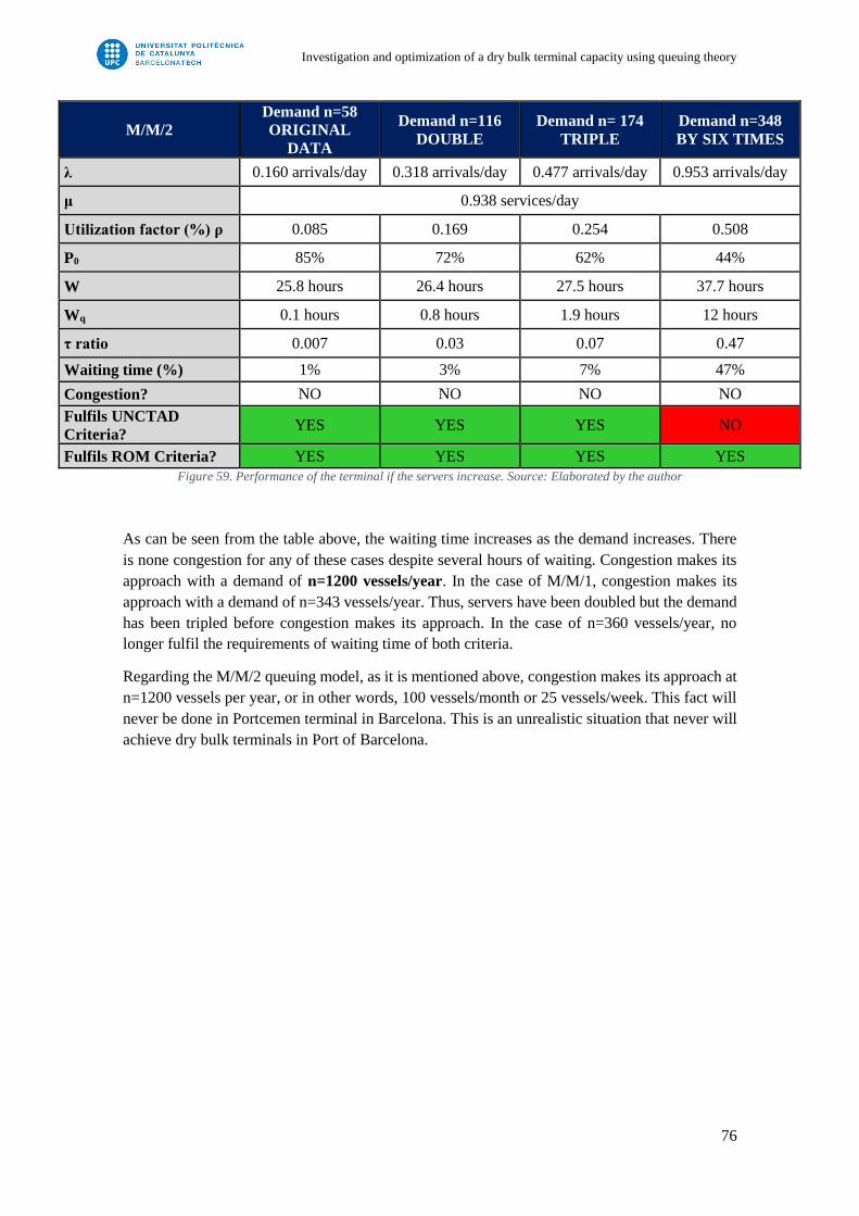
Investigation and optimization of a dry bulk terminal capacity using queuing theory
76
M/M/2
Demand n=58
ORIGINAL
DATA
Demand n=116
DOUBLE
Demand n= 174
TRIPLE
Demand n=348
BY SIX TIMES
λ 0.160 arrivals/day 0.318 arrivals/day 0.477 arrivals/day 0.953 arrivals/day
μ 0.938 services/day
Utilization factor (%) ρ 0.085 0.169 0.254 0.508
P0 85% 72% 62% 44%
W 25.8 hours 26.4 hours 27.5 hours 37.7 hours
Wq 0.1 hours 0.8 hours 1.9 hours 12 hours
τ ratio 0.007 0.03 0.07 0.47
Waiting time (%) 1% 3% 7% 47%
Congestion? NO NO NO NO
Fulfils UNCTAD
Criteria? YES YES YES NO
Fulfils ROM Criteria? YES YES YES YES
Figure 59. Performance of the terminal if the servers increase. Source: Elaborated by the author
As can be seen from the table above, the waiting time increases as the demand increases. There
is none congestion for any of these cases despite several hours of waiting. Congestion makes its
approach with a demand of n=1200 vessels/year. In the case of M/M/1, congestion makes its
approach with a demand of n=343 vessels/year. Thus, servers have been doubled but the demand
has been tripled before congestion makes its approach. In the case of n=360 vessels/year, no
longer fulfil the requirements of waiting time of both criteria.
Regarding the M/M/2 queuing model, as it is mentioned above, congestion makes its approach at
n=1200 vessels per year, or in other words, 100 vessels/month or 25 vessels/week. This fact will
never be done in Portcemen terminal in Barcelona. This is an unrealistic situation that never will
achieve dry bulk terminals in Port of Barcelona.

Investigation and optimization of a dry bulk terminal capacity using queuing theory
77
5. DISCUSSION AND CONCLUSIONS
This minor thesis has provided an analysis on the performance of the Portcemen Terminal in Port
of Barcelona. The main objective of this thesis was to characterize and analyze the fulfilment of
Portcemen terminal in Barcelona Port applying the queuing theory in order to investigate the
service levels using standard design parameters of ROM and UNCTAD. Moreover, the sub-goal
of the thesis was to carry out a resilience study of the cement terminal in Barcelona Port through
performance indicators and raising various scenarios. The conclusions obtained are presented
below.
Terminal performance:
It was assumed that the population size is unlimited and so it is the capacity of the service. Thus,
there is no restriction on the capacity of the system and it can be an infinite waiting line. So we
could assert that the notation of the Queuing Theory Model assumed in this cement terminal is
M/M/1/infinite/FIFO (M/M/1).
With the calculations of the parameters for this queuing model for the demand in 2015, it can be
asserted that it is an over dimensioned system. With a demand of 58 vessels per year in 2015, the
probability of the system being empty is extremely high (83%) and the probability of having one
vessel in the system is only 14%. The terminal receives on average 1.10 arrivals/week, or in other
words 4.75 arrivals/month. With only 1 loading and unloading equipment, the number of services
if the server is occupied is 1 service/day approximately with an average duration of 25.6
hours/service.
Nevertheless, it has to be borne in mind that the traffic in 2015 was only the 60% approximately
of the traffic before the financial crisis of 2008 in Spain that represented one of the most
significant setback in global trade. Yet, maritime shipping is subject to fluctuations as commercial
opportunities change. This is an added difficulty of predicting traffic to dimensioning maritime
terminals. Although Portcemen terminal is not one of the biggest cement terminals in the world,
for sure it has had and it will have greater volume of dry bulk traffic than it has now.
Through the manual simulation of the terminal based on the data provided by Portcemen that
simulates the dynamics of the terminal during year 2015, it could be analysed the performance of
such terminal. With the arrival times and the service times determined, the simulation could
proceed in order to acquire the departure times. Thus, it can be seen how many vessels might wait
in queue for the service. The results obtained, considering some assumptions which have to be
done due to the lack of information, show that the maximum number of vessels that overlap in
the same day is 2. This fact only happens in 4 different occasions during this year, where these
vessels have to wait on average 15 hours to be served. All year round, there are 307 days in which
no vessels arrived, 54 days that served 1 vessel and 4 days that overlap 2 vessels in the same day.
Every service lasts 25.6 hours in average, meaning that the server is working 17% of the time in
a year. This fact reflects again that most time of the year the terminal is empty.
Moreover, on the basis of data compiled, inter-arrivals time have been calculated. The minimum
inter-arrival time is 1 day whereas the maximum inter-arrival time is 26 days. As can be seen, the
arrivals are totally stochastic and extremely variables. Although the larger vessels have real

Investigation and optimization of a dry bulk terminal capacity using queuing theory
78
scheduled arrivals, the smaller ones do not. It was necessary in this minor thesis to assume the
random nature of the arrivals in case of non-programmed calls. Accordingly, the minimum service
time is 7 hours whereas the maximum service time is 55 hours.
Levels of service:
Terminal capacity calculations provide a link between the level of service achieved and the
demand placed, the capacity provided and the performance expected. When planning facilities, it
is necessary to try out different capacities with different traffic forecasts for different points of
time. This calculation will be used for setting performance (productivity), proposed capacity
(number of berths) and varying traffic demand to determine the effect on level of service (ship
waiting time).
According to Spanish Recommendations on Maritime Works (ROM 2.0-11), the service quality
level (𝜏) is defined as relative waiting or average waiting time of ships in port before being
assigned a berth due to the occupancy of all berths divided by the average total time of the vessels
moored at the berth or time of service. This ratio is widely used as a measure of the level of service
provided by a terminal. For this reason, it has been applied in the present thesis in order to analyze
the performance of the terminal considering the average waiting time in queue (Wq) and service
time (μ). Once the value of the ratio (𝜏) is obtained, it has been be compared with the criteria of
admissible waiting time defined by UNCTAD and with the one defined by ROM.
In year 2015, with a demand of n=58 vessels/year, such ratio (𝜏) is 0.2 so there is no congestion
and both criteria of admissible waiting time are fulfilled. It can be asserted that the terminal in
2015 works in a low level of capacity.
A study of resilience has been carried out to analyze eventual scenarios that may occur in the
future. For this, the parameters for other selected model have been calculated. The proposed
scenarios that have been analyzed in the thesis are increasing the demand and increasing the
number of servers.
Increasing the demand
In this case, the demand has been increased to double and triple so it can be seen when the current
system collapse. The results obtained are summarized in the table below.
M/M/1 Demand n=58
ORIGINAL DATA
Demand n=116
DOUBLE
Demand n= 174
TRIPLE
Demand n=343
CONGESTION
Utilization factor (%) ρ 17% 34% 51% 100%
τ ratio 0.2 0.5 1 -422
Congestion? NO NO NO YES
Fulfils UNCTAD Criteria? YES NO NO NO
Fulfils ROM Criteria? YES YES NO NO
Figure 60. Summary of the performance of the terminal if the demand increases. Source: Elaborated by the author

Investigation and optimization of a dry bulk terminal capacity using queuing theory
79
Predictably, the probability of the system being empty decreases as the demand increases whereas
the probability of having n vessels in the system increases exponentially as the demand increases.
Moreover, both number of clients and average waiting time raise along with the demand. As can
be seen, there is none congestion for any of these cases despite several hours of waiting.
Congestion makes its approach with a demand of n=343 vessels/year. It is almost a vessel per day
served when the system collapses.
While the congestion factor determined through Queuing Theory Method implies a fully
inoperative state of the terminal, the lack of fulfilment of the waiting time criteria imply an
inadequate performance of the terminal, but not necessarily that the terminal is not operative or
congested.
In this sense, it is observed how the different levels of restriction of the different criteria for
waiting time, (being UNCTAD criteria more restrictive), lead to scenarios when one of the
waiting time criteria (ROM) is fulfilled and other (UNCTAD) is not, as it is the case of n=116 for
M/M/1 model. For this case, it should be recommended to improve the conditions of it so as to
ensure the availability of a higher number of service channels, which at the same time would
require further research, due to the variability of the traffic.
In the case of tripling the demand, no longer fulfil the requirements of waiting time of both
criteria. However, the system is not congested yet.
Increasing the servers
In this case, the server has been increased to double so it can be seen the performance of the
terminal with a queuing model M/M/2. Simultaneously, the demand will be multiplied by 2, 3
and 6 times. The results obtained are summarized in the table below.
M/M/2 Demand n=58
ORIGINAL DATA
Demand n=116
DOUBLE
Demand n= 174
TRIPLE
Demand n=348
BY SIX TIMES
Utilization factor (%) ρ 9% 17% 25% 51%
τ ratio 0.007 0.03 0.07 0.47
Congestion? NO NO NO NO
Fulfils UNCTAD Criteria? YES YES YES NO
Fulfils ROM Criteria? YES YES YES YES
Figure 61. Summary of the performance of the terminal if the servers increase. Source: Elaborated by the author
By analysing the probability of the system being empty and the probability of having n vessels in
the system in the case of having 2 servers compared to 1 server, both of them are practically
identical having a demand of n=58 vessels. It makes sense since in case of having only 1 server,
with a demand of 58 vessels, the system operates well below its maximum capacity before
congestion. So with 2 servers only one of them will work most of the time because it is capable
to absorb all the demand whereas the other one will remain empty the most of the time.

Investigation and optimization of a dry bulk terminal capacity using queuing theory
80
There is none congestion for any of these cases despite several hours of waiting. Congestion
makes its approach with a demand of n=1200 vessels/year, or in other words, 100 vessels/month
or 25 vessels/week. This fact will never be done in Portcemen terminal in Barcelona. This is an
unrealistic situation that never will achieve dry bulk terminals in Port of Barcelona. In the case of
M/M/1, congestion makes its approach with a demand of n=343 vessels/year. Thus, servers have
been doubled but the demand has been tripled before congestion makes its approach. In the case
of n=360 vessels/year, no longer fulfil the requirements of waiting time of both criteria.
Investigation and optimization of a dry bulk terminal capacity using queuing theory
81
BIBLIOGRAPHY
[1] UNCTAD, United Nations Conference on Trade and Development, 1985, Chapter II: Planning
Principles. Port Development: A Handbook for Planners in Developing Countries.
[2] UNCTAD, United Nations Conference on Trade and Development, 1974. Review of Maritime
Transport (Review of current and long-term aspects of maritime transport).
[3] UNCTAD, United Nations Conference on Trade and Development, 1985. Development and
Improvement of ports. Development of Bulk Terminals.
[4] Puertos del Estado, 2012. Recomendaciones para obras marítimas, ROM 2.0-11, Tomo I.
Recomendaciones para el proyecto y ejecución en Obras de Atraque y Amarre.
[5] UNCTAD, United Nations Conference on Trade and Development, 2017. Review of maritime
transport.
[6] UNCTAD, United Nations Conference on Trade and Development, 1996, Port Management
Series, Vol. 4. Port Organization and Management.
[7] Portcemen, S.A., 2011. Memoria de Responsabilidad Social.
[8] Van Vianen, T., 2015. Delft University of Technology. Simulation-integrated Design of Dry
Bulk Terminals.
[9] Jingjing, X., & Dong, L., 2012. Systems Engineering Procedia, 4, 345–351. Queuing Models
to Improve Port Terminal Handling Service.
[10] El-Naggar M. E., 2010. Journal of Soil Science and Environmental Management, 1(4), 77-
85. Application of queuing theory to the container terminal at Alexandria seaport
[11] Kuo T., Huang W., Wu S., Cheng P., 2006. Journal of Marine Science and Technology,
14(3), 155-164. A case study of inter-arrival time distributions of container ships.
[12] Worthington, D., 1996. Journal of the Operational Research Society, Vol. 47, pp. 1423–1424.
An Introduction to Queueing Theory
[13] Willig A., 1999. Technical University Berlin, Telecommunication Networks Group. A short
introduction to queuing theory.
[14] Tipper, D. University of Pittsburg. Graduate Telecommunications and Networking Program.
Basic queues.
[15] Duran E., 2015. Universitat Politècnica de Catalunya, Departamento de Ciencia e Ingeniería
Náuticas. Dimensioning and optimization of operations for dry bulk terminals.
[16] López, E., 2016. Universitat Politècnica de Catalunya, M.S.c. Coastal and Marine
Engineering and Management. Service levels at container terminals of Barcelona Port
Authority.
[17] Zoran R., Branislav D., 2005. Inf. Manage Sci., 16(3), pp. 1-16. Optimal Number and
Capacity of Servers in Queuing Systems.
[18] Noritake M., Kimura S., 1983. Journal of Watwerway Port Coastal and Ocean Engineering,
Vol. 109, No. 3, pp. 323-329. Optimum Number and Capacity of Seaport Berth.
Investigation and optimization of a dry bulk terminal capacity using queuing theory
82
[19] Corbet J. J., Winebrake J., 2008. Global Forum on Transport and Environment in a
Globalizing World. Energy and Environmental Research Associates. The Impacts of
Globalization on International Maritime Transport Activity.
[20] Bornozis N., 2006. A review of dry bulk sector. Dry bulk shipping: The engine of global
trade.
[21] Rodrigue J.P., Browne M., 2014. Transport Geographies: An introduction, Blackwell
Publishing. Chapter 10. International Maritime Freight Transport and Logistics.
[22] Ligthart, A., 2016. Cement Distribution Consultants. Intercem Americas. Global cement
trade flows and US imports.
[23] Ligthart, A., 2017. Cement Distribution Consultants. Intercem Shipping. Current
developments in the cement and clinker shipping.
[24] Ligthart, A., 2018. Cement Distribution Consultants. Intercem Shipping Forum. Export
Markets for European cement – a shipping perspective.
[25] Ligthart, A., 2014. Cement Distribution Consultants. Intercem Shipping Forum. Who
controls cement and clinker shipping?
[26] Ligthart, A., 2015. Cement Distribution Consultants. Intercem Shipping Forum. Size and
capabilities of global export, import and Distribution terminals for cement and clinker.
[27] Puertos del Estado. Statistics on the traffic on Spanish Ports. http://www.puertos.es/es-
es/estadisticas/RestoEstad%C3%ADsticas/Paginas/Resto-estadisticas.aspx. Visited on June
2018.
[28] Autoritat Portuaria de Barcelona (APB). El puerto, Negocios, Mapas, Estadísticas.
http://www.portdebarcelona.cat/es/web/port-dels-negocis/servicio-de-atencion-al-cliente.
Visited on June 2018.
[29] Portcemen Terminal S,A. http://www.portcemen.com. Visited on May 2018.
[30] Cement Distribution Consultants. Industry Information, Consulting Services.
https://cementdistribution.com. Visited on May 2018.
[31] Agrupación de fabricantes de cemento de España, Oficemen. Informes estadísticos, Anuario
del sector cementero español. https://www.oficemen.com. Visited on July 2018.
[32] Baltic Dry Index (BDI). https://es.investing.com/indices/baltic-dry-chart. Visited on July
2018.
[33] Confederación Española de Asociaciones de Fabricantes de Productos de Construcción.
Información del sector, Producción y consumo de cemento. http://www.cepco.es. Visited
on July 2018.
[34] The Geography of Transport Systems. Maritime Transportation, Transportation Terminals.
https://transportgeography.org. Visited on July 2018.

Investigation and optimization of a dry bulk terminal capacity using queuing theory
83
ANNEX
84
Table of Contents
A. EVOLUTION OF SOLID BULK CARGO BY AUTHORITY PORT IN TONS .............. 85
B. QUEUING THEORY FORMULAS ...................................................................................... 86
C. CHARACTERISTICS OF THE VESSELS SERVED IN PORTCEMEN TERMINAL IN
2015 ............................................................................................................................................. 90
D. IMAGES OF THE VESSELS SERVED IN PORTCEMEN TERMINAL IN 2015 ............. 92
E. DRY BULK CARGO TERMINAL, PLANNING CHARTS .............................................. 117
F. TABLES OF SMIRNOV-KOLMOGOROV TEST ............................................................. 119

85
A. EVOLUTION OF SOLID BULK CARGO BY AUTHORITY PORT IN TONS
Annual evolution of solid bulk cargo in Spain by Authority Port in tons (2005-2017). Source: Puertos del Estado
Port Authority 2005 2006 2007 2008 2009 2010 2011 2012 2013 2014 2015 2016 2017 TOTAL
BY AAPP A CORUÑA 4.437.796 4.095.639 4.140.677 3.289.608 3.215.589 3.191.581 3.470.995 4.179.771 3.688.168 4.310.507 4.912.338 4.345.101 5.057.024 52.334.794
ALICANTE 1.667.536 1.642.514 1.569.601 1.086.515 1.111.169 723.273 720.512 717.061 940.343 1.109.761 1.244.009 1.904.456 1.877.179 16.313.929
ALMERIA 6.306.756 5.964.929 6.065.259 4.906.958 3.291.672 3.213.116 3.930.994 4.703.570 4.151.806 4.406.405 5.762.813 4.695.167 5.622.006 63.021.451
AVILES 3.082.731 3.615.486 3.451.464 3.114.668 2.293.135 2.746.802 3.297.196 3.393.152 2.797.247 3.012.751 3.260.161 2.920.900 2.874.981 39.860.675
BAHIA DE ALGECIRAS 2.652.263 2.708.226 2.679.852 1.588.521 1.743.479 1.475.224 1.563.349 1.955.220 1.597.565 1.603.174 2.130.519 1.778.840 1.942.451 25.418.683
BAHIA DE CADIZ 2.557.442 2.699.354 4.405.625 2.117.801 1.636.990 1.687.143 1.851.089 1.815.381 1.867.533 1.776.315 1.623.696 1.763.516 1.747.593 27.549.478
BALEARES 2.318.339 2.188.436 2.314.781 2.130.632 1.689.471 1.859.831 1.643.380 1.623.778 1.309.549 1.319.455 1.215.735 1.550.899 1.610.653 22.774.939
BARCELONA 4.051.927 4.107.582 3.870.253 3.506.472 3.921.099 3.542.218 3.544.297 4.685.744 4.373.720 4.764.706 4.426.087 4.430.798 4.465.644 53.690.547
BILBAO 4.261.127 5.524.178 5.832.384 5.266.459 3.827.983 4.451.915 4.000.342 4.261.691 4.421.587 4.593.976 4.528.219 4.362.064 4.543.171 59.875.096
CARTAGENA 5.082.060 5.173.022 5.371.083 4.628.556 3.615.556 3.114.236 3.653.775 4.880.341 4.519.222 5.308.274 5.554.193 5.304.817 5.820.153 62.025.288
CASTELLON 3.293.591 3.590.891 3.902.855 4.017.009 1.865.858 2.941.178 3.244.831 3.114.303 3.102.799 4.192.762 4.636.911 5.198.982 6.463.715 49.565.685
CEUTA 71.229 66.793 75.637 71.772 68.226 141.410 142.108 150.350 63.426 32.645 25.625 22.249 21.900 953.370
FERROL-SAN CIBRAO 8.289.621 8.709.257 8.726.704 9.781.089 9.268.088 7.435.083 8.685.748 10.505.475 8.999.195 9.498.616 9.839.879 9.406.039 10.455.814 119.600.608
GIJON 19.658.167 18.298.185 18.305.091 16.869.645 12.456.055 13.401.423 12.573.625 14.482.418 14.947.162 16.218.571 18.905.283 16.023.647 19.192.104 211.331.376
HUELVA 7.512.508 7.394.282 7.603.640 6.525.092 4.180.685 5.394.260 4.502.005 4.830.967 4.145.909 4.662.814 5.137.350 5.759.383 6.487.394 74.136.289
LAS PALMAS 1.772.615 1.678.836 1.615.745 1.139.545 753.111 738.740 524.432 375.490 364.102 477.533 483.909 534.113 500.380 10.958.551
MALAGA 2.100.473 1.953.430 1.603.906 1.342.750 766.796 772.746 893.662 782.253 868.836 1.095.103 1.370.093 1.748.149 1.675.098 16.973.295
MARIN 1.016.241 891.966 937.575 847.406 879.867 960.542 853.558 805.966 826.305 853.972 998.817 1.047.281 915.820 11.835.315
MELILLA 84.427 45.826 51.655 34.112 32.782 43.257 33.395 20.779 9.000 6.815 3.425 5.825 7.372 378.670
MOTRIL 1.246.697 1.172.380 973.264 756.864 453.149 473.242 608.379 547.036 479.197 430.807 452.358 451.149 404.311 8.448.833
PASAIA 3.281.138 3.248.288 2.778.170 2.351.378 1.649.664 1.655.965 1.246.600 1.419.971 1.212.240 1.509.001 1.694.292 1.099.170 834.439 23.980.316
STA. CRUZ DE TENERIFE 1.892.082 1.986.964 1.716.058 1.352.468 848.311 818.565 782.167 567.440 488.158 437.559 406.750 414.999 413.555 12.125.076
SANTANDER 5.139.652 4.164.897 4.374.837 3.732.466 2.919.749 2.879.604 3.060.049 3.236.676 2.988.773 3.189.256 3.518.578 2.823.113 3.428.750 45.456.400
SEVILLA 2.788.885 2.827.598 2.343.706 2.344.193 2.421.146 2.133.427 1.997.898 1.813.175 1.824.074 1.739.610 2.073.690 2.250.277 2.201.621 28.759.300
TARRAGONA 11.903.296 11.237.751 13.626.199 12.420.882 9.830.390 9.452.166 9.279.089 10.888.789 7.375.070 9.708.015 8.391.029 9.065.474 9.515.688 132.693.838
VALENCIA 6.360.690 7.148.231 7.322.671 5.165.374 3.523.706 2.591.139 2.374.045 2.177.058 2.444.573 2.680.192 2.684.864 2.531.577 2.278.857 49.282.977
VIGO 692.535 701.899 632.226 458.180 381.302 459.139 433.320 303.132 289.478 299.331 287.939 234.910 261.609 5.435.000
VILAGARCIA 578.235 613.257 570.068 506.221 488.175 409.144 339.355 346.675 202.966 323.047 403.439 320.553 421.100 5.522.236
TOTAL TONS OF SOLID
BULK 114.100.059 113.450.097 116.860.986 101.352.636 79.133.203 78.706.369 79.250.195 88.583.662 80.298.003 89.560.973 95.972.002 91.993.448 101.040.382 1.230.302.015

86
B. QUEUING THEORY FORMULAS
M/M/1 Queuing System Formulas
𝜌 =𝜆
𝜇
𝑃𝑛 = (1 − 𝜌) · 𝜌𝑛
𝑃0 = 1 − 𝜌
𝐿 =𝜌
1 − 𝜌=
𝜆
𝜇 − 𝜆
𝐿𝑞 =𝜆2
𝜇 · (𝜇 − 𝜆)=
𝜌2
1 − 𝜌
𝑊 =𝐿
𝜆=
1
𝜇 − 𝜆
𝑊𝑞 =𝜌
𝜇 − 𝜆
𝜂 =𝜌
1 − 𝜌
𝑃(𝑛 ≥ 𝑋) = 𝜌𝑋
𝑃(𝑊 > 𝑡) = 𝑒−𝜇(1−𝜌)𝑡
𝑃(𝑊𝑞 > 𝑡) = 𝜌 · 𝑒−𝜇(1−𝜌)𝑡
𝑃(𝑋 = 𝑥) =𝜆𝑋
𝑥!· 𝑒−𝜆
𝑃(𝑋 = 𝑥) = 𝜇 · 𝑒−𝜇𝑥
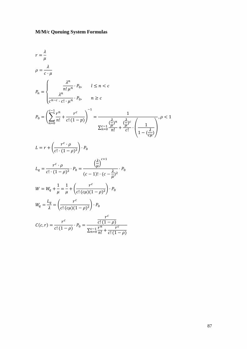
87
M/M/c Queuing System Formulas
𝑟 =𝜆
𝜇
𝜌 =𝜆
𝑐 · 𝜇
𝑃𝑛 =
{
𝜆𝑛
𝑛! 𝜇𝑛· 𝑃0, 𝑙 ≤ 𝑛 < 𝑐
𝜆𝑛
𝑐𝑛−𝑐 · 𝑐! · 𝜇𝑛· 𝑃0, 𝑛 ≥ 𝑐
𝑃0 = (∑𝑟𝑛
𝑛!+
𝑟𝑐
𝑐! (1 − 𝑝)
𝑐−1
𝑛=0
)
−1
=1
∑(𝜆𝜇)𝑛
𝑛!+(𝜆𝜇)𝑐
𝑐!· (
1
1 − (𝜆𝑐𝜇))𝑐−1
𝑛=0
, 𝜌 < 1
𝐿 = 𝑟 + (𝑟𝑐 · 𝜌
𝑐! · (1 − 𝜌)2) · 𝑃0
𝐿𝑞 =𝑟𝑐 · 𝜌
𝑐! · (1 − 𝜌)2· 𝑃0 =
(𝜆𝜇)𝑐+1
(𝑐 − 1)! · (𝑐 −𝜆𝜇)2· 𝑃0
𝑊 = 𝑊𝑞 +1
𝜇=1
𝜇+ (
𝑟𝑐
𝑐! (𝑐𝜇)(1 − 𝜌)2) · 𝑃0
𝑊𝑞 =𝐿𝑞𝜆= (
𝑟𝑐
𝑐! (𝑐𝜇)(1 − 𝜌)2) · 𝑃0
𝐶(𝑐, 𝑟) =𝑟𝑐
𝑐! (1 − 𝜌)· 𝑃0 =
𝑟𝑐
𝑐! (1 − 𝜌)
∑𝑟𝑛
𝑛!+
𝑟𝑐
𝑐! (1 − 𝜌)𝑐−1𝑛=0

88
M/D/1 Queuing System Formulas
𝐿 = 𝜌 +1
2(𝜌2
1 − 𝜌)
𝐿𝑞 =1
2(𝜌2
1 − 𝜌)
𝑊 =1
𝜇+
𝜌
2𝜇(1 − 𝜌)
𝑊𝑞 =𝜌
2𝜇(1 − 𝜌)

89
Relationships between random variables
𝐿 = 𝜆 · 𝑊
𝐿𝑞 = 𝜆 · 𝑊𝑞
𝑊 = 𝑊𝑞 +1
𝜇
𝑟 = 𝐿 − 𝐿𝑞 = 𝜆 · (𝑊 −𝑊𝑞) =𝜆
𝜇
𝐿𝑞 = 𝐿 − (1 − 𝑃0)
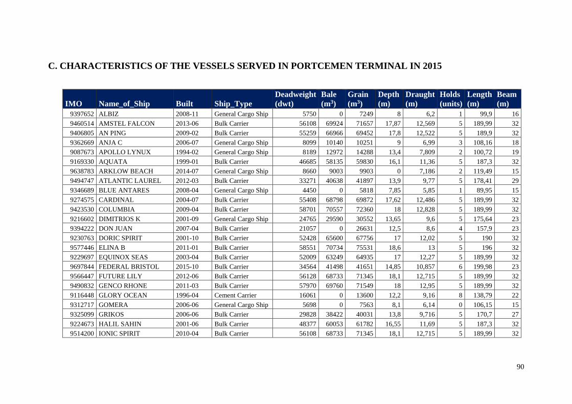
90
C. CHARACTERISTICS OF THE VESSELS SERVED IN PORTCEMEN TERMINAL IN 2015
IMO Name_of_Ship Built Ship_Type
Deadweight
(dwt)
Bale
(m3)
Grain
(m3)
Depth
(m)
Draught
(m)
Holds
(units)
Length
(m)
Beam
(m)
9397652 ALBIZ 2008-11 General Cargo Ship 5750 0 7249 8 6,2 1 99,9 16
9460514 AMSTEL FALCON 2013-06 Bulk Carrier 56108 69924 71657 17,87 12,569 5 189,99 32
9406805 AN PING 2009-02 Bulk Carrier 55259 66966 69452 17,8 12,522 5 189,9 32
9362669 ANJA C 2006-07 General Cargo Ship 8099 10140 10251 9 6,99 3 108,16 18
9087673 APOLLO LYNUX 1994-02 General Cargo Ship 8189 12972 14288 13,4 7,809 2 100,72 19
9169330 AQUATA 1999-01 Bulk Carrier 46685 58135 59830 16,1 11,36 5 187,3 32
9638783 ARKLOW BEACH 2014-07 General Cargo Ship 8660 9003 9903 0 7,186 2 119,49 15
9494747 ATLANTIC LAUREL 2012-03 Bulk Carrier 33271 40638 41897 13,9 9,77 5 178,41 29
9346689 BLUE ANTARES 2008-04 General Cargo Ship 4450 0 5818 7,85 5,85 1 89,95 15
9274575 CARDINAL 2004-07 Bulk Carrier 55408 68798 69872 17,62 12,486 5 189,99 32
9423530 COLUMBIA 2009-04 Bulk Carrier 58701 70557 72360 18 12,828 5 189,99 32
9216602 DIMITRIOS K 2001-09 General Cargo Ship 24765 29590 30552 13,65 9,6 5 175,64 23
9394222 DON JUAN 2007-04 Bulk Carrier 21057 0 26631 12,5 8,6 4 157,9 23
9230763 DORIC SPIRIT 2001-10 Bulk Carrier 52428 65600 67756 17 12,02 5 190 32
9577446 ELINA B 2011-01 Bulk Carrier 58551 70734 75531 18,6 13 5 196 32
9229697 EQUINOX SEAS 2003-04 Bulk Carrier 52009 63249 64935 17 12,27 5 189,99 32
9697844 FEDERAL BRISTOL 2015-10 Bulk Carrier 34564 41498 41651 14,85 10,857 6 199,98 23
9566447 FUTURE LILY 2012-06 Bulk Carrier 56128 68733 71345 18,1 12,715 5 189,99 32
9490832 GENCO RHONE 2011-03 Bulk Carrier 57970 69760 71549 18 12,95 5 189,99 32
9116448 GLORY OCEAN 1996-04 Cement Carrier 16061 0 13600 12,2 9,16 8 138,79 22
9312717 GOMERA 2006-06 General Cargo Ship 5698 0 7563 8,1 6,14 0 106,15 15
9325099 GRIKOS 2006-06 Bulk Carrier 29828 38422 40031 13,8 9,716 5 170,7 27
9224673 HALIL SAHIN 2001-06 Bulk Carrier 48377 60053 61782 16,55 11,69 5 187,3 32
9514200 IONIC SPIRIT 2010-04 Bulk Carrier 56108 68733 71345 18,1 12,715 5 189,99 32
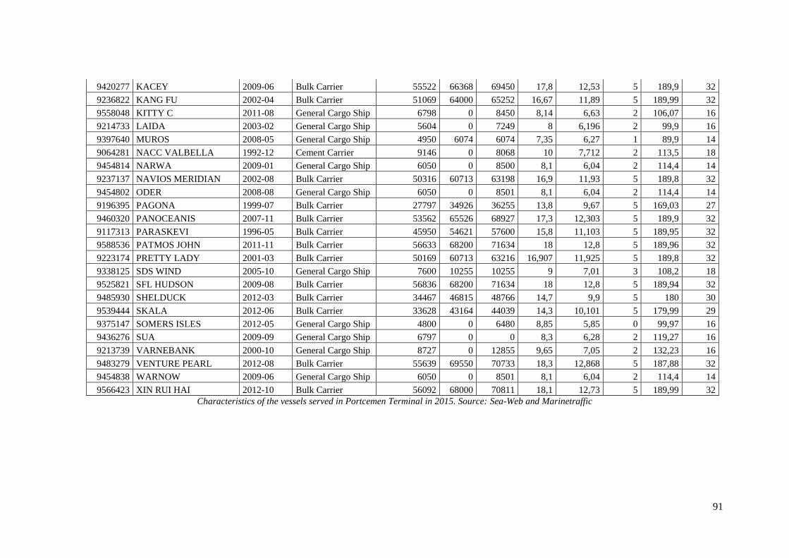
91
9420277 KACEY 2009-06 Bulk Carrier 55522 66368 69450 17,8 12,53 5 189,9 32
9236822 KANG FU 2002-04 Bulk Carrier 51069 64000 65252 16,67 11,89 5 189,99 32
9558048 KITTY C 2011-08 General Cargo Ship 6798 0 8450 8,14 6,63 2 106,07 16
9214733 LAIDA 2003-02 General Cargo Ship 5604 0 7249 8 6,196 2 99,9 16
9397640 MUROS 2008-05 General Cargo Ship 4950 6074 6074 7,35 6,27 1 89,9 14
9064281 NACC VALBELLA 1992-12 Cement Carrier 9146 0 8068 10 7,712 2 113,5 18
9454814 NARWA 2009-01 General Cargo Ship 6050 0 8500 8,1 6,04 2 114,4 14
9237137 NAVIOS MERIDIAN 2002-08 Bulk Carrier 50316 60713 63198 16,9 11,93 5 189,8 32
9454802 ODER 2008-08 General Cargo Ship 6050 0 8501 8,1 6,04 2 114,4 14
9196395 PAGONA 1999-07 Bulk Carrier 27797 34926 36255 13,8 9,67 5 169,03 27
9460320 PANOCEANIS 2007-11 Bulk Carrier 53562 65526 68927 17,3 12,303 5 189,9 32
9117313 PARASKEVI 1996-05 Bulk Carrier 45950 54621 57600 15,8 11,103 5 189,95 32
9588536 PATMOS JOHN 2011-11 Bulk Carrier 56633 68200 71634 18 12,8 5 189,96 32
9223174 PRETTY LADY 2001-03 Bulk Carrier 50169 60713 63216 16,907 11,925 5 189,8 32
9338125 SDS WIND 2005-10 General Cargo Ship 7600 10255 10255 9 7,01 3 108,2 18
9525821 SFL HUDSON 2009-08 Bulk Carrier 56836 68200 71634 18 12,8 5 189,94 32
9485930 SHELDUCK 2012-03 Bulk Carrier 34467 46815 48766 14,7 9,9 5 180 30
9539444 SKALA 2012-06 Bulk Carrier 33628 43164 44039 14,3 10,101 5 179,99 29
9375147 SOMERS ISLES 2012-05 General Cargo Ship 4800 0 6480 8,85 5,85 0 99,97 16
9436276 SUA 2009-09 General Cargo Ship 6797 0 0 8,3 6,28 2 119,27 16
9213739 VARNEBANK 2000-10 General Cargo Ship 8727 0 12855 9,65 7,05 2 132,23 16
9483279 VENTURE PEARL 2012-08 Bulk Carrier 55639 69550 70733 18,3 12,868 5 187,88 32
9454838 WARNOW 2009-06 General Cargo Ship 6050 0 8501 8,1 6,04 2 114,4 14
9566423 XIN RUI HAI 2012-10 Bulk Carrier 56092 68000 70811 18,1 12,73 5 189,99 32
Characteristics of the vessels served in Portcemen Terminal in 2015. Source: Sea-Web and Marinetraffic
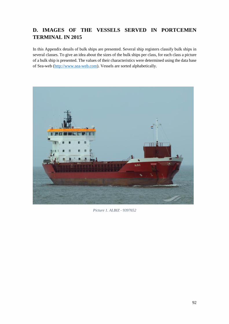
92
D. IMAGES OF THE VESSELS SERVED IN PORTCEMEN
TERMINAL IN 2015
In this Appendix details of bulk ships are presented. Several ship registers classify bulk ships in
several classes. To give an idea about the sizes of the bulk ships per class, for each class a picture
of a bulk ship is presented. The values of their characteristics were determined using the data base
of Sea-web (http://www.sea-web.com). Vessels are sorted alphabetically.
Picture 1. ALBIZ - 9397652
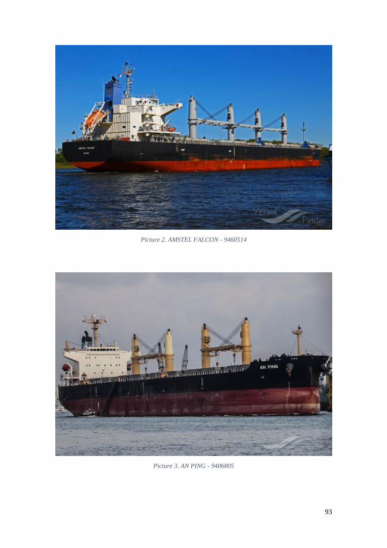
93
Picture 2. AMSTEL FALCON - 9460514
Picture 3. AN PING - 9406805
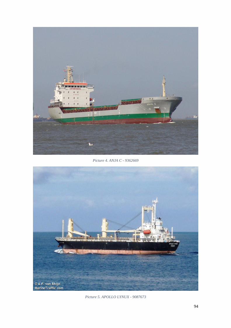
94
Picture 4. ANJA C - 9362669
Picture 5. APOLLO LYNUX - 9087673
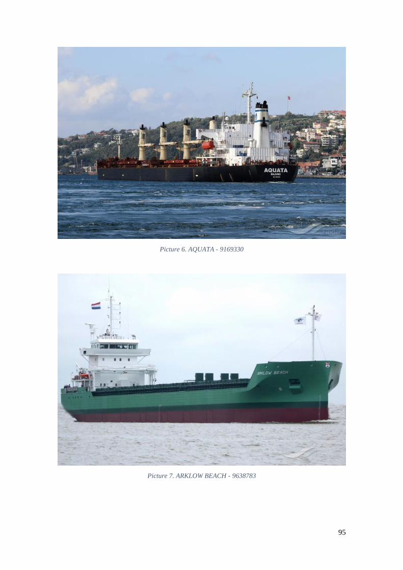
95
Picture 6. AQUATA - 9169330
Picture 7. ARKLOW BEACH - 9638783

96
Picture 8. ATLANTIC LAUREL - 9494747
Picture 9. BLUE ANTARES - 9346689

97
Picture 10. CARDINAL - 9274575
Picture 11. COLUMBIA - 9423530
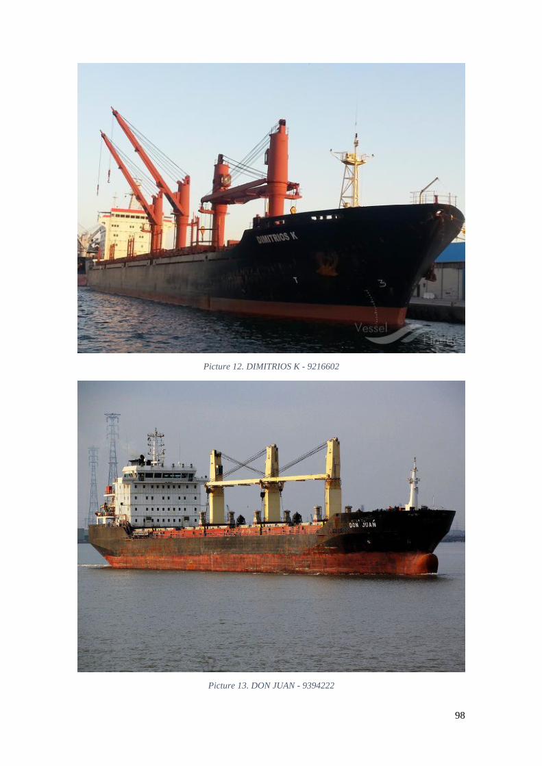
98
Picture 12. DIMITRIOS K - 9216602
Picture 13. DON JUAN - 9394222
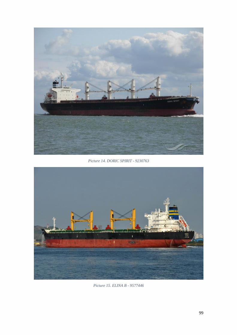
99
Picture 14. DORIC SPIRIT - 9230763
Picture 15. ELINA B - 9577446
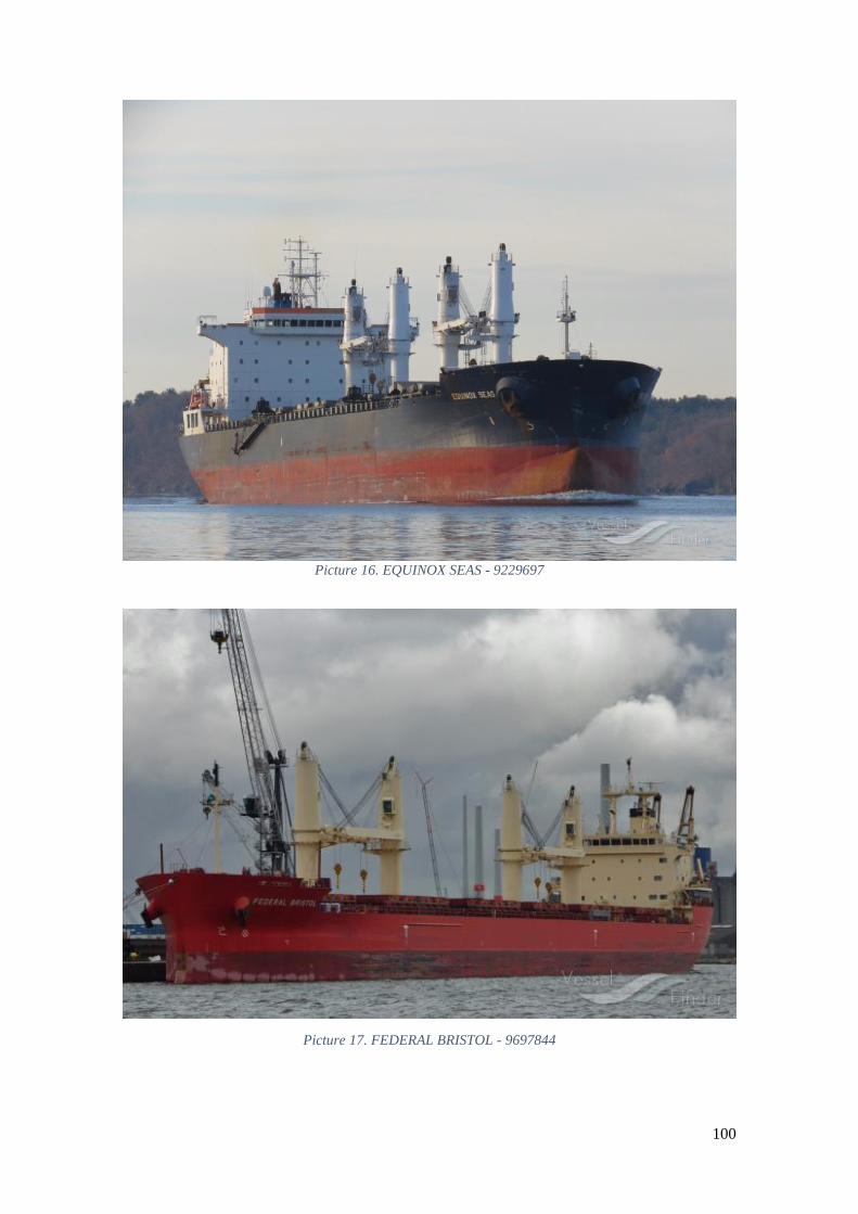
100
Picture 16. EQUINOX SEAS - 9229697
Picture 17. FEDERAL BRISTOL - 9697844
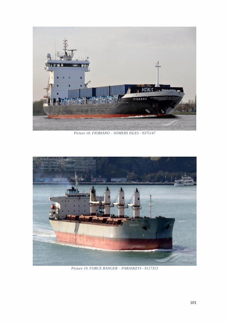
101
Picture 18. FIORIANO – SOMERS ISLES - 9375147
Picture 19. FORCE RANGER – PARASKEVI - 9117313
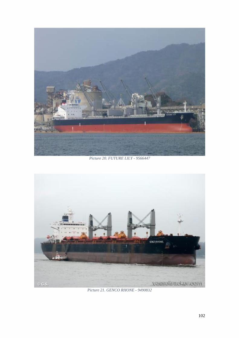
102
Picture 20. FUTURE LILY - 9566447
Picture 21. GENCO RHONE - 9490832
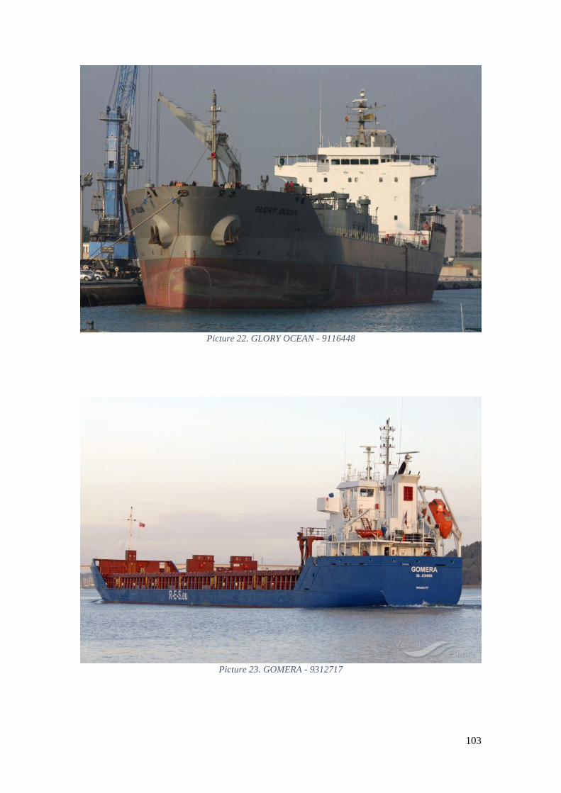
103
Picture 22. GLORY OCEAN - 9116448
Picture 23. GOMERA - 9312717
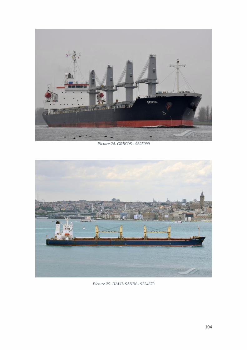
104
Picture 24. GRIKOS - 9325099
Picture 25. HALIL SAHIN - 9224673

105
Picture 26. KACEY - 9420277
Picture 27. KANG FU - 9236822

106
Picture 28. KITTY C - 9558048
Picture 29. LAIDA - 9214733
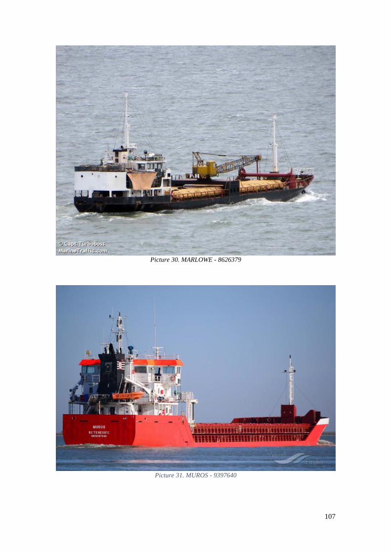
107
Picture 30. MARLOWE - 8626379
Picture 31. MUROS - 9397640

108
Picture 32. MV IONIC SPIRIT - 9514200
Picture 33. NARWA - 9454814

109
Picture 34. NAVIOS MERIDIAN - 9237137
Picture 35. ODER - 9454802
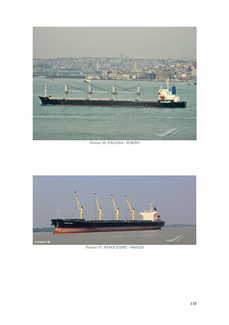
110
Picture 36. PAGONA - 9196395
Picture 37. PANOCEANIS - 9460320

111
Picture 38. PORTOROZ – PATMOS JOHN - 9588536
Picture 39. PRETTY LADY - 9223174
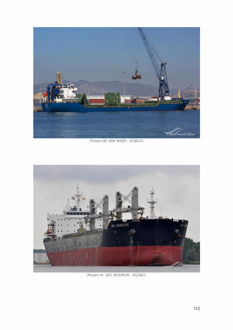
112
Picture 40. SDS WIND - 9338125
Picture 41. SFL HUDSON - 9525821
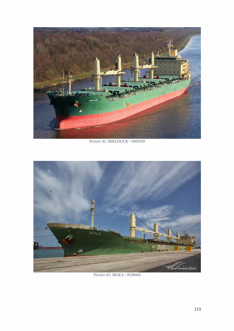
113
Picture 42. SHELDUCK - 9485930
Picture 43. SKALA - 9538444

114
Picture 44. SUA - 9436276
Picture 45. VALBELLA - 9064281

115
Picture 46. VARNEBANK - 9213739
Picture 47. VENTURE PEARL - 9483279

116
Picture 48. WARNOW - 9454838
Picture 49. XIN RUI HAI - 9566423
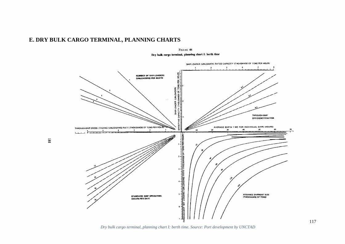
117
E. DRY BULK CARGO TERMINAL, PLANNING CHARTS
Figure 1. Dry bulk cargo terminal, planning chart I: berth time. Source: Port development by UNCTAD
Dry bulk cargo terminal, planning chart I: berth time. Source: Port development by UNCTAD
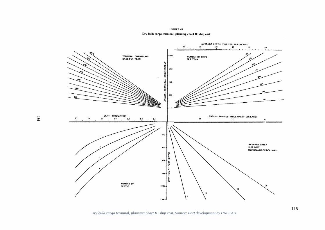
118
Dry bulk cargo terminal, planning chart II: ship cost. Source: Port development by UNCTAD
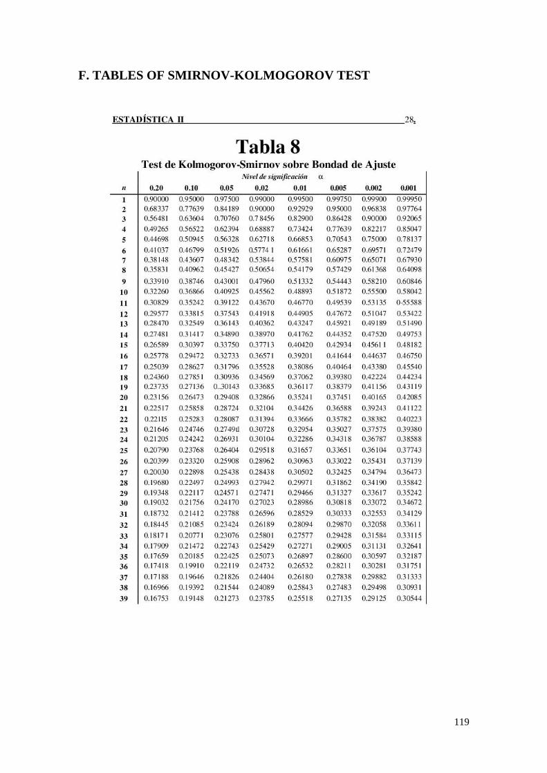
119
F. TABLES OF SMIRNOV-KOLMOGOROV TEST

120

121