investigation into heating and hyperfine loss mechanisms in magnetically...
TRANSCRIPT

Investigation into Heating and Hyperfine Loss Mechanisms inMagnetically Trapped Ultra-Cold Rubidium
by
Chenchong Zhu
A THESIS SUBMITTED IN PARTIAL FULFILLMENT
OF THE REQUIREMENTS FOR THE DEGREE OF
Bachelor of Science
in
THE FACULTY OF SCIENCE
(Physics and Astronomy)
The University Of British Columbia
(Vancouver)
April 2010
c© Chenchong Zhu, 2010

Abstract
This thesis describes our investigation into elastic collisions between an ultra-cold, magnetically
trapped atom ensemble of rubidium-87 or rubidium-85, and background, room-temperature rubid-
ium. We investigated two specific phenomena: low scattering angle elastic collisions that change
the trapped ensemble energy distribution without resulting in immediate trap loss, or “heating col-
lisions”, and the dependence of elastic collisional loss cross-sections on the hyperfine state of the
trapped rubidium ensemble. A theoretical description of quantum scattering theory is given, along
with how this theory can be utilized to calculate heating collision rates. A theoretical and technical
description of our rubidium magnetic/magneto-optical trap follows, including descriptions of two
new additions to the system: an RF coil and a Zeeman optical pumping system. We then describe
the methods used to experimentally determine trap loss rates and the energy distribution in the trap.
Our results show that the average rate of energy imparted to a trapped atom in our system is on
the order of 1 µK per second. We also show that the Rb-Rb loss rate slope 〈σv〉 is independent
of hyperfine state, indicating that any loss dependency on hyperfine state rests with collisions with
other species, or other forms of loss.
Revision: ubcdiss.cls r26
ii

Table of Contents
Abstract . . . . . . . . . . . . . . . . . . . . . . . . . . . . . . . . . . . . . . . . . . . . . ii
Table of Contents . . . . . . . . . . . . . . . . . . . . . . . . . . . . . . . . . . . . . . . iii
List of Tables . . . . . . . . . . . . . . . . . . . . . . . . . . . . . . . . . . . . . . . . . . vi
List of Figures . . . . . . . . . . . . . . . . . . . . . . . . . . . . . . . . . . . . . . . . . vii
Acknowledgments . . . . . . . . . . . . . . . . . . . . . . . . . . . . . . . . . . . . . . . xiii
1 Introduction . . . . . . . . . . . . . . . . . . . . . . . . . . . . . . . . . . . . . . . . 11.1 Overview . . . . . . . . . . . . . . . . . . . . . . . . . . . . . . . . . . . . . . . 1
1.2 Background . . . . . . . . . . . . . . . . . . . . . . . . . . . . . . . . . . . . . . 1
1.3 Motivation for Studying Trap Loss . . . . . . . . . . . . . . . . . . . . . . . . . . 2
1.4 Motivation for Our Work . . . . . . . . . . . . . . . . . . . . . . . . . . . . . . . 2
2 Theory . . . . . . . . . . . . . . . . . . . . . . . . . . . . . . . . . . . . . . . . . . . 62.1 Collision Mechanics . . . . . . . . . . . . . . . . . . . . . . . . . . . . . . . . . 7
2.1.1 Energy Imparted to Trapped Atoms From Collisions . . . . . . . . . . . . 7
2.1.2 Determining Laboratory Frame Scattering Angle . . . . . . . . . . . . . . 8
2.2 Rate Equations . . . . . . . . . . . . . . . . . . . . . . . . . . . . . . . . . . . . 9
2.3 Trapped Atom Heating . . . . . . . . . . . . . . . . . . . . . . . . . . . . . . . . 11
2.4 Scattering Amplitude . . . . . . . . . . . . . . . . . . . . . . . . . . . . . . . . . 12
2.4.1 Determining the Scattering Amplitude . . . . . . . . . . . . . . . . . . . . 12
2.4.2 The S, K and T Matrix Values . . . . . . . . . . . . . . . . . . . . . . . . 14
2.5 Other Forms of Collisions . . . . . . . . . . . . . . . . . . . . . . . . . . . . . . 15
3 Experimental Apparatus Background . . . . . . . . . . . . . . . . . . . . . . . . . . 163.1 The Magneto-Optical Trap . . . . . . . . . . . . . . . . . . . . . . . . . . . . . . 16
3.2 The Magnetic Trap . . . . . . . . . . . . . . . . . . . . . . . . . . . . . . . . . . 18
3.2.1 Magnetic Trap Potential . . . . . . . . . . . . . . . . . . . . . . . . . . . 19
iii

3.2.2 Magnetic Trap Majorana Losses . . . . . . . . . . . . . . . . . . . . . . . 21
3.3 RF Coil-Induced Hyperfine Transitions . . . . . . . . . . . . . . . . . . . . . . . 22
3.4 Zeeman-Optical Pumping . . . . . . . . . . . . . . . . . . . . . . . . . . . . . . . 24
4 The Miniature Atom Trap (MAT) . . . . . . . . . . . . . . . . . . . . . . . . . . . . 274.1 Vacuum System . . . . . . . . . . . . . . . . . . . . . . . . . . . . . . . . . . . . 27
4.2 Rubidium Injection System . . . . . . . . . . . . . . . . . . . . . . . . . . . . . . 28
4.3 Imaging Systems . . . . . . . . . . . . . . . . . . . . . . . . . . . . . . . . . . . 29
4.3.1 Photodiode . . . . . . . . . . . . . . . . . . . . . . . . . . . . . . . . . . 29
4.3.2 CCD Camera . . . . . . . . . . . . . . . . . . . . . . . . . . . . . . . . . 31
4.3.3 Webcam . . . . . . . . . . . . . . . . . . . . . . . . . . . . . . . . . . . . 31
4.4 Laser Systems . . . . . . . . . . . . . . . . . . . . . . . . . . . . . . . . . . . . . 31
4.5 The Magnetic Coils . . . . . . . . . . . . . . . . . . . . . . . . . . . . . . . . . . 32
4.6 The RF Knife . . . . . . . . . . . . . . . . . . . . . . . . . . . . . . . . . . . . . 32
4.7 The Zeeman-Optical Pumping System . . . . . . . . . . . . . . . . . . . . . . . . 33
5 Numerical Methods and Results . . . . . . . . . . . . . . . . . . . . . . . . . . . . . 375.1 Loss Cross-Section Calculator . . . . . . . . . . . . . . . . . . . . . . . . . . . . 37
5.2 Magnetic Trap Simulator . . . . . . . . . . . . . . . . . . . . . . . . . . . . . . . 38
5.2.1 Overview of the Simulator . . . . . . . . . . . . . . . . . . . . . . . . . . 38
5.2.2 Changes in the Scattering Amplitude due to Varying the C12 Coefficient . . 38
5.3 Multi-Channel Loss Cross-Section Calculator . . . . . . . . . . . . . . . . . . . . 39
6 Procedure and Experimental Results . . . . . . . . . . . . . . . . . . . . . . . . . . . 426.1 General Procedure . . . . . . . . . . . . . . . . . . . . . . . . . . . . . . . . . . 42
6.2 Measurement of Trap Energy Distribution . . . . . . . . . . . . . . . . . . . . . . 45
6.3 Measurement of Heated Fraction . . . . . . . . . . . . . . . . . . . . . . . . . . . 45
6.3.1 Relationship Between Heated Fraction and Trap Depth . . . . . . . . . . . 48
6.3.2 Relationship Between Heated Fraction and Rb Number Density . . . . . . 54
6.4 Measurement of Pure State Loss Rate vs. Rb Pressure . . . . . . . . . . . . . . . . 57
6.5 Anomalous Results . . . . . . . . . . . . . . . . . . . . . . . . . . . . . . . . . . 57
7 Discussion . . . . . . . . . . . . . . . . . . . . . . . . . . . . . . . . . . . . . . . . . 637.1 Measurement of Heated Fraction . . . . . . . . . . . . . . . . . . . . . . . . . . . 63
7.2 Measurement of Pure State Loss Rate vs. Rb Pressure . . . . . . . . . . . . . . . . 64
7.3 Anomalous Results . . . . . . . . . . . . . . . . . . . . . . . . . . . . . . . . . . 67
7.4 Conclusion . . . . . . . . . . . . . . . . . . . . . . . . . . . . . . . . . . . . . . 67
8 Appendix . . . . . . . . . . . . . . . . . . . . . . . . . . . . . . . . . . . . . . . . . . 68
iv

8.1 List of Data Files Used . . . . . . . . . . . . . . . . . . . . . . . . . . . . . . . . 68
Bibliography . . . . . . . . . . . . . . . . . . . . . . . . . . . . . . . . . . . . . . . . . . 69
v
List of Tables
2.1 Table of atomic units, and their equivalent SI values, from [26]. Often, a value in
atomic units will simply be given the label a.u., rather than dimensions such as Bohr
radii or Hartrees. . . . . . . . . . . . . . . . . . . . . . . . . . . . . . . . . . . . 6
2.2 A table of calculated CM and laboratory frame scattering angles for Rb-Ar colli-
sions. Energy scale is the energy imparted to the trapped atom (U). θ is CM scat-
tering angle, and Θ is laboratory frame scattering angle. All values were calculated
assuming background Ar has an initial velocity vBg = 353.09 m/s (most probable
velocity at 300 K). . . . . . . . . . . . . . . . . . . . . . . . . . . . . . . . . . . 8
2.3 A table of calculated CM and laboratory frame scattering angles for Rb-Rb colli-
sions. Energy scale is the energy imparted to the trapped atom (U). θ is CM scat-
tering angle, and Θ is laboratory frame scattering angle. All values were calculated
assuming background Rb has an initial velocity vBg = 239.42 m/s (most probable
velocity at 300 K). . . . . . . . . . . . . . . . . . . . . . . . . . . . . . . . . . . 9
2.4 A table presenting estimated values for the CM θdi f f of Rb-Ar and Rb-Rb collisions,
calculated using Eq. 2.7. The de Broglie wavelength calculated assumes the CM
relative velocity in the collision is given by vmost probable =√
2kBT/mBg, where T =
300 K. σtotal is estimated from 〈σtotalv〉/vmean, where vmean =√
8kBT/πmBg (T =
300 K). . . . . . . . . . . . . . . . . . . . . . . . . . . . . . . . . . . . . . . . . 9
6.1 Table of Gnuplot fit results for the FH curves in Fig. 6.6. . . . . . . . . . . . . . . 49
6.2 Table of Gnuplot fit results for the relationship between FH rate (denoted F ′H) and
MOT loading rate R, for Fig. 6.10. The leftmost 2 mK point was not used in the
best fit of the 2 mK data. The relationship between d 〈E〉/dt (denoted 〈E ′〉) and
MOT loading rate R is also given for each trap in accordance with Eq. 6.4. . . . . . 57
6.3 Table of Gnuplot linear best fit results for data plotted in Figs. 6.12 and 6.13. Within
error, the slopes of both states match for both 85Rb and 87Rb, as predicted by nu-
merical calculation. . . . . . . . . . . . . . . . . . . . . . . . . . . . . . . . . . . 58
vi

List of Figures
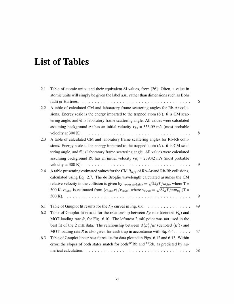
1.1 Semi-log plot of Rb-Ar 〈σv〉 versus trap depth. (〈σv〉 is defined in Eq. 2.13, and
is linearly proportional loss rate.) to The blue line is the numerically calculated〈σv〉, while the magenta points are experimentally determined. The blue, horizontal
dashed line is the numerically calculated 〈σv〉 at zero trap depth (i.e. the Boltzmann
average of the total collisional cross section multiplied by v). The single point to the
far right was determined using the MOT, while the magnetic trap was used for the
other points to the left. The three points near 2 - 10 mK are systematically upward
deviated. . . . . . . . . . . . . . . . . . . . . . . . . . . . . . . . . . . . . . . . . 4
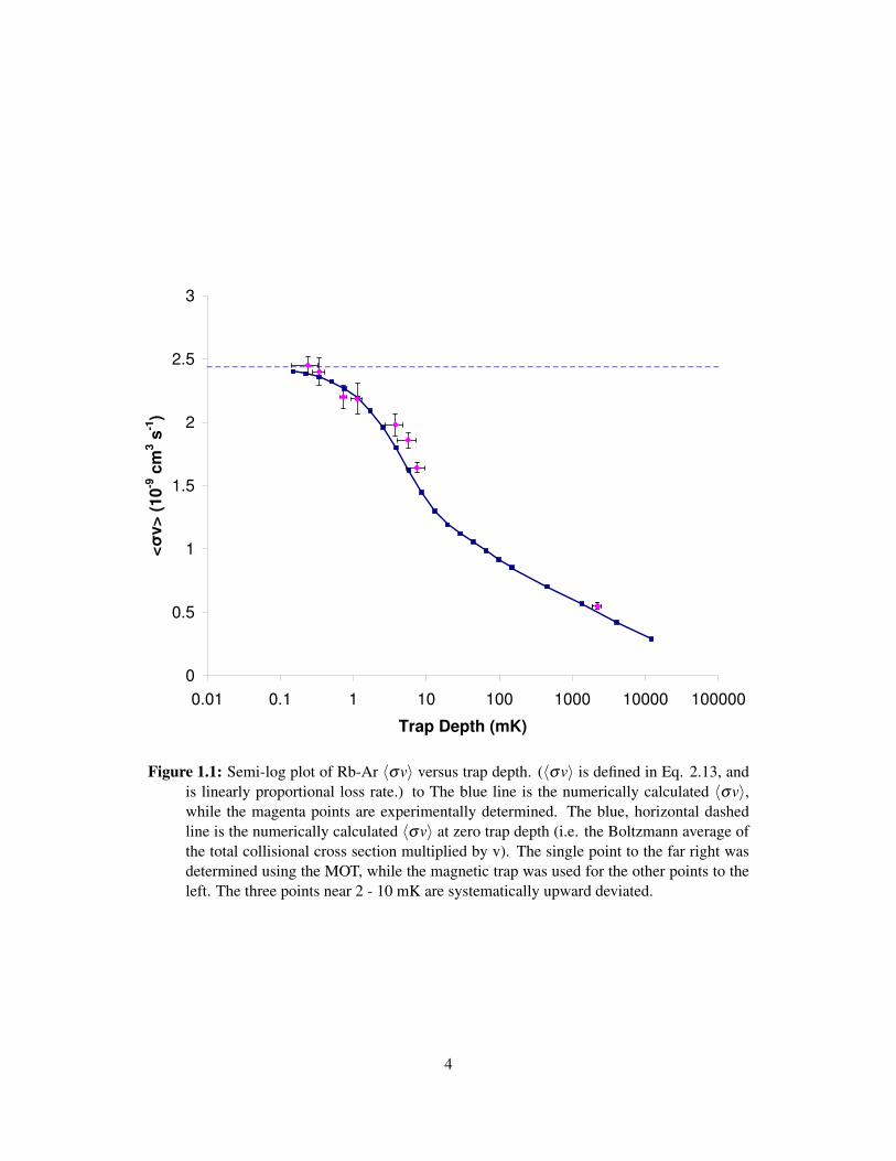
1.2 Semi-log plot of Rb-Rb 〈σv〉 versus trap depth. (〈σv〉 is defined in Eq. 2.13, and is
linearly proportional loss rate.) The brown line is the numerically calculated 〈σv〉,while the magenta points are experimentally determined. The brown, horizontal
dashed line is the numerically calculated 〈σv〉 at zero trap depth (i.e. the Boltzmann
average of the total collisional cross section multiplied by v). The number density
of Rb is known only up to a constant scaling factor, and the experimental points
were artificially rescaled using a constant scaling factor to fit on the theoretical line.
Following rescaling the two follow each other closely, except for the 1800 mK MOT
point, which is significantly larger than theoretical calculations. This is likely due
to excited state collisions not accounted for in theory that significantly increase the
value of 〈σv〉. . . . . . . . . . . . . . . . . . . . . . . . . . . . . . . . . . . . . . 5
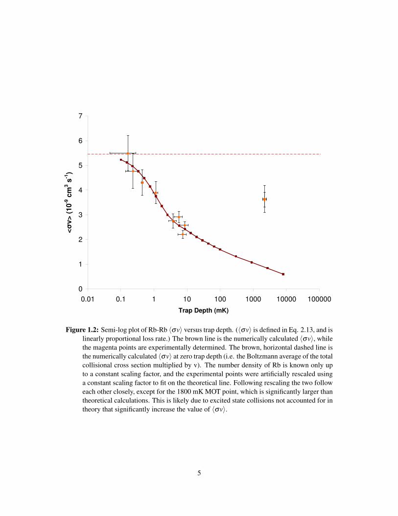
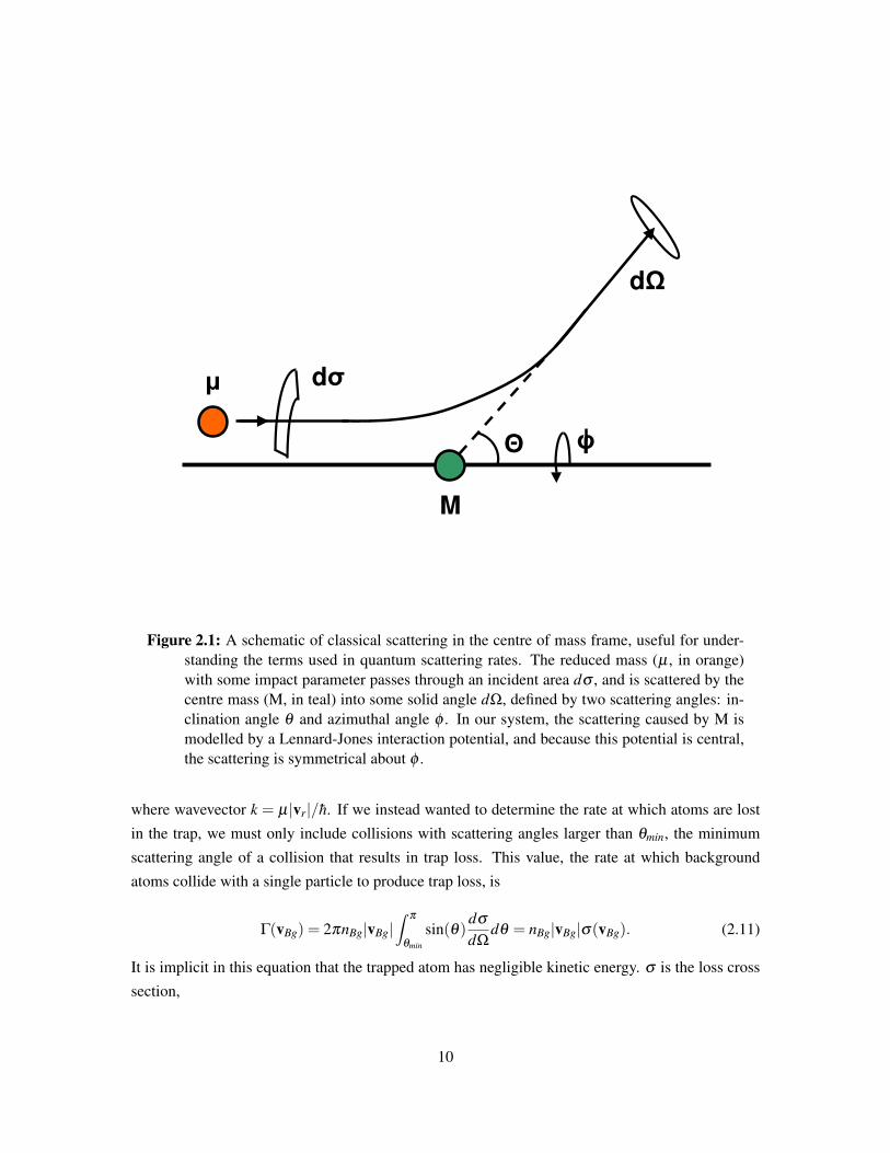
2.1 A schematic of classical scattering in the centre of mass frame, useful for under-
standing the terms used in quantum scattering rates. The reduced mass (µ , in
orange) with some impact parameter passes through an incident area dσ , and is
scattered by the centre mass (M, in teal) into some solid angle dΩ, defined by two
scattering angles: inclination angle θ and azimuthal angle φ . In our system, the
scattering caused by M is modelled by a Lennard-Jones interaction potential, and
because this potential is central, the scattering is symmetrical about φ . . . . . . . . 10
vii

3.1 A diagram of the position-dependent forces in a magneto-optical trap. σ+ circularly
polarized light drives 52S1/2 |F = 2 mF〉 → 52P3/2 |F ′ = 2 mF +1〉, and σ− circu-
larly polarized light drives 52S1/2 |F = 2 mF〉 → 52P3/2 |F ′ = 2 mF −1〉. The Zee-
man splitting caused by the position-dependent magnetic field from the quadrupole
coils brings the σ+ light further from its corresponding transition, and the σ− light
closer to its corresponding transition, when z > 0, When z < 0, the opposite is the
case. Because one laser is preferentially absorbed over the other at different points
in the trap, the forces between the two lasers are imbalanced. The MOT is designed
such that this imbalance drives atoms back into the centre of the trap. Diagram from
[13], courtesy of David Fagnan. . . . . . . . . . . . . . . . . . . . . . . . . . . . 18
3.2 A Breit-Rabi diagram of the Zeeman splitting of 87Rb 52S1/2 |F = 2〉. The hyperfine
states corresponding to each Zeeman-hyperfine splitting are labelled on the right.
The energy shift at B = 0 is the shift for the |F = 2〉 hyperfine splitting from the
52S1/2 fine splitting of 87Rb. The weak-field seeking, or diamagnetic, states are|2 2〉, |2 1〉, and |2 0〉. This figure was created using [17]. . . . . . . . . . . . . . . 21
3.3 A diagram of a transition from 87Rb |1 −1〉 to |1 0〉. The RF knife couples the two
hyperfine states at a point x where the difference in Zeeman splitting curves is hνRF .
Atoms ejected from the |1 −1〉 state at x are at potential E (E < hνRF ), and thereby
atoms that can reach potential E are eventually lost from the trap due to the RF knife. 23
3.4 A diagram showing how difficult it would be to use the RF knife to transition a
trapped 87Rb |2 2〉 atom to untrappable state |2 −1〉, as described by Bouyer et al..
Three transitions would have to be made before the atom is ejected. The probability
of ever reaching the |2 −1〉 or lower is less than 10% [6]. . . . . . . . . . . . . . . 24
3.5 A schematic of the Zeeman pumping process described in Section 3.4, showing a
few possible transition paths for a trapped atom. Each bar is a hyperfine state with
some F and mF number indicated by the labels. Red arrows are transitions due to
the laser, and blue arrows are spontaneous emission transitions. For example, an
atom starts in |2 0〉. σ+ pump laser light excites it to |2′ 1〉, from which it can decay
to any of the 52S1/2 states shown, including the desired |2 2〉. If the decay is to |1 1〉,then σ+ repump light boosts it to |2′ 2〉, where it can potentially drop to |2 2〉. All
other possible decay paths of the excited atom are accounted for by the pump and
repump beams such that the |2 2〉 becomes the most likely final state of any trapped
atom. . . . . . . . . . . . . . . . . . . . . . . . . . . . . . . . . . . . . . . . . . 26
4.1 A simplified schematic of the MAT magneto-optical/magnetic trap. Diagram from
[13], courtesy of David Fagnan. . . . . . . . . . . . . . . . . . . . . . . . . . . . 28
viii

4.2 A photograph of the MAT, labelled to indicate significant components of the system.
The insert photo is a close-up of the MAT components surrounding the vacuum cell. 29
4.3 An example of an Rb equilibration curve. MOT loading rate R is used as a proxy for
Rb background number density. An exponential decay has been fitted to the data,
indicating that R decreases exponentially from a t = 0 value of (8.15±0.11)×107
s−1 to a steady state value of (9.249±0.084)×106 s−1. . . . . . . . . . . . . . . . 30
4.4 A plot of RF amplitude as a function of RF frequency νRF . The amplitude remains
relatively constant except in the region of 0 - 2 MHz and past 115 - 120 MHz. . . . 33
4.5 A plot of the fraction of the 87Rb |F = 1〉 and |F = 2〉 atoms loaded into the mag-
netic trap from a MOT as a function of magnetic coil current, experimentally de-
termined in order to find the optimal currents for spin filtering. For |F = 1〉, only|1 −1〉 is trappable. For |F = 2〉, |2 2〉 becomes trappable at ∼0.3 A, and |2 1〉 at
∼0.6 A. |2 0〉, not shown here, becomes trappable at ∼7 A. . . . . . . . . . . . . . 35
4.6 A plot of the fraction of the 85Rb |F = 3〉 and |F = 2〉 atoms loaded into the mag-
netic trap from a MOT as a function of magnetic coil current, experimentally deter-
mined in order to find the optimal currents for spin filtering. For |F = 3〉, |3 3〉 is
trappable at∼0.2 A, |3 2〉 at∼0.4 A, |3 1〉 at∼0.85 A, and |3 0〉 (not shown) at∼4.5
A. For |F = 2〉, |2 −2〉 becomes trappable at ∼0.3 A, and |2 −1〉 at ∼0.85 A. No
data exists for |2 0〉, theoretically estimated to be trappable at currents past ∼7 A. . 36
5.1 A semilog plot of numerically determined σ (loss cross-section) and σtotal , for col-
lisions between trapped Rb and background Rb travelling at 293 m/s, as functions
of C12 value. σ is calculated for a 1 K trap. The value of both σ (loss cross-section)
and σtotal are constant to within ∼ 10% until C12 ≥∼ 5×10¹⁰ atomic units. . . . . 40
5.2 A semilog plot of numerically determined | f (k,θ)|2 as a function of θ for collisions
between trapped Rb and background Rb travelling at 293 m/s. Each curve was
calculated using a different C12, noted in the legend in atomic units. As C12 value
increases, the number of oscillations seen in the | f (k,θ)|2 curve decreases. . . . . . 41
6.1 An example of a MOT loading curve. The curve is produced by (1) starting with a
steady-state MOT ensemble, (2) turning off the magnetic field for 500 ms to eject
the ensemble, and then (3) turning the field back on and letting the trap load once
again. The fluorescence seen by the photodiode is not zero when there is no trapped
ensemble at (2) because some laser light still scatters off the MAT vacuum cell. The
resulting curve is an exponential rise from the zero-level at (2) to the MOT steady
state fluorescence. . . . . . . . . . . . . . . . . . . . . . . . . . . . . . . . . . . . 43
ix

6.2 An example of a series of magnetic trap loss-determination curves. Each curve
(taking the orange curve as our example) begin with a steady state MOT (1). We
then cool the atoms, and turn off the lasers while simultaneously ramping up the
magnetic field gradient in 7.5 ms. If Zeeman pumping is used, it is performed im-
mediately after that for 200 ms. Once this is complete, the trap is left to evolve on
its own (2) for some designated time (during which the lasers are off, so no fluores-
cence reaches the photodiode). At the end of this time, the magnetic field is ramped
back down over 15 ms, the lasers are flashed back on, taking a measurement of the
ensemble fluorescence (3), before the magnetic fields are turned off to empty the
trap. The magnetic fields are then turned on, creating a MOT loading curve (4).
Each of these loss-determination curves determines a single value on a magnetic
trap loss curve (the multicoloured diamonds on each curve), which can be strung to-
gether to create an exponential decay. Note that the MOT steady state value appears
to increase over time - this is possibly due to heating of the magnetic coils. Because
we normalize point (3) to the MOT steady state fluorescence to produce a trapped
fraction, small amounts of deviation such as seen in this graph can be neglected. . . 44
6.3 Cumulative energy distribution curves of an 87Rb |1 −1〉 3.14±0.84 mK magnetic
trap at various hold times (denoted in the legend), determined by 125 ms RF sweeps
at varying lower frequencies. Each data point on a distribution curve indicates the
fraction of atoms trapped with some particular energy (in MHz) or lower (at some
time). Over 8000 ms, the total number of trapped atoms decreased by more than
33% (each curve is normalized to the total number of atoms in the trap at the time
to eliminate trap loss biases), but no discernable heating is seen. . . . . . . . . . . 46
6.4 Cumulative energy distribution curves of an 87Rb |1 −1〉 3.14±0.84 mK magnetic
trap at various hold times (denoted in the legend), determined by 125 ms RF sweeps
at varying lower frequencies. The RF knife was also used to eliminate all atoms
of energy 8 MHz or above at the beginning of each trap hold. Each data point
on a distribution curve indicates the fraction of atoms trapped with some particular
energy (in MHz) or lower (at some time). Over 8000 ms, the total number of trapped
atoms decreased by more than 20% (each curve is normalized to the total number
of atoms in the trap at the time to eliminate trap loss biases). This lower loss rate
may be because the average energy of the trapped atoms is lower and therefore more
incoming collisions result in heating rather than trap loss, but due to the significant
increase in noise in the distributions it is not possible to determine if any heating
has actually occured. . . . . . . . . . . . . . . . . . . . . . . . . . . . . . . . . . 47
x

6.5 Plot of FH vs. magnetic trap hold time for 87Rb |1 −1〉 in a 1.3± 0.14 mK trap.
Magnetic coil gradient was set to 5 A, but the 1.3 mK trap depth was set by a
continuous RF sweep from 27.53 MHz to 90 MHz over the magnetic trap hold
time. An initial RF sweep was used to eliminate all atoms of energy 7.96± 0.87
MHz (0.382±0.042 mK) or lower. The error shown is derived from best fitting for
the trapped fraction, and is not a measure of the shot noise of the points. A linear
best fit performed on Gnuplot, plotted here in magenta, gave an initial fraction of
0.1473±0.0077, and a slope of 0.0073±0.0012 s−1. Using Eq. 6.3, this gives us a
heating rate per atom of ∼0.2 MHz s−1, or ∼9 µK s−1. . . . . . . . . . . . . . . . 49
6.6 Plot of FH vs. magnetic trap hold time for 87Rb |1 −1〉 curves for traps of varying
depth. Magnetic coil gradient was set to 7 A, but the trap depth was set by a contin-
uous RF sweeps. The four depths used were 19.8±1.6 MHz (0.949±0.074 mK),
29.5±2.3 MHz (1.41±0.11 mK), 39.1±3.1 MHz (1.88±0.15 mK) and 57.9±4.6
MHz (2.78±0.22 mK). Emid was set to 13.9±1.1 MHz (0.667±0.053 mK). Error
bars for 19.8 and 57.9 MHz FH curves are included to give a visual example of the
level of shot noise in the system. . . . . . . . . . . . . . . . . . . . . . . . . . . . 50
6.7 Plot of Fig. 6.6 FH best fit slopes vs. trap depth. . . . . . . . . . . . . . . . . . . . 51
6.8 Plot of Fig. 6.6 FH best fit slopes vs. 〈qv〉 - 〈qv〉m. To determine 〈qv〉 and 〈qv〉m, the
estimate 〈qv〉 = 〈σtotalv〉 - 〈σv〉 was used. Theoretically, the relationship between
the two values is, to first order, linear, and the slope is nBg. A linear best fit to the
data was performed in Gnuplot, and is plotted alongside the data. The fit’s slope is
4.07±0.75×106 cm−3 and intercept is 0.00141±0.00073 s−1. . . . . . . . . . . 52
6.9 Plot of Fig. 6.6 FH initial value (best fit y-intercept) vs. trap depth. . . . . . . . . . 53
6.10 Plot of the relationship between FH rate and MOT loading rate R for a 1.30±0.14
mK trap and 2.00±0.22 mK trap (set using continuous RF knife sweeps with lower
frequencies 27.53 and 42.72 MHz, respectively). Emid was set to 0.667±0.053 mK.
These data points were determined by performing Gnuplot best fits on FH curves
taken over a number of R values. . . . . . . . . . . . . . . . . . . . . . . . . . . . 55
6.11 Plot of the relationship between FH(t = 0) initial fraction and MOT loading rate R
for a 1.30±0.14 mK trap and 2.00±0.22 mK trap (set using continuous RF knife
sweeps with lower frequencies 27.53 and 42.72 MHz, respectively). Emid was set to
0.667±0.053 mK. These data points were determined by performing Gnuplot best
fits on FH curves taken over a number of R values. . . . . . . . . . . . . . . . . . . 56
xi

6.12 Plot of total loss rate Γ vs. MOT loading rate R for 85Rb |3 3〉 and |2 −2〉 in mag-
netic traps. Trapping current was set to 2.2 A (a 2.83± 0.77 mK trap) for |3 3〉,and 3.4 A (a 2.83± 0.74 mK trap) for |2 −2〉. The RF knife was not used. While
there is a y-intercept (Γ(R = 0)) difference between the two lines, their slopes are
identical, within error. Linear best fits determined using Gnuplot have been plotted
alongside experimental data. . . . . . . . . . . . . . . . . . . . . . . . . . . . . . 59
6.13 Plot of total loss rate Γ vs. MOT loading rate R for 87Rb |2 2〉 and |1 −1〉 in mag-
netic traps. Trapping current was set to 4.53 A (a 2.83±0.74 mK trap) for |1 −1〉,and 2.2 A (a 2.83±0.77 mK trap) for |2 2〉. The RF knife was not used. While there
is small a y-intercept (Γ(R = 0)) difference between the two lines, their slopes are
identical, within error. Linear best fits determined using Gnuplot have been plotted
alongside experimental data. . . . . . . . . . . . . . . . . . . . . . . . . . . . . . 60
6.14 An investigation into rapid intial losses from an 87Rb |1 −1〉 magnetic trap. The
trap depth is kept either at 1.00±0.15 mK using the magnetic coils alone at 1.815
A, or at 1 mK using a combination of an RF sweep from 21.0944 MHz to 100 MHz
and the magnetic coils at currents 2.5 A or higher. Long-term losses look identical,
but a rapid initial loss can be seen for high-currents. Note that at 12 A the trapped
fraction reduces to just a few percent in under 2 seconds - this does not occur in an
identical trap (using RF sweeping to hold the trap depth) where Zeeman pumping is
not used! . . . . . . . . . . . . . . . . . . . . . . . . . . . . . . . . . . . . . . . . 61
6.15 A plot of ΓRIL, obtained by fitting exponential decays to the fast initial losses, as a
function of A−1 (instead of A; see Section 7.3). Unfortunately, the resulting data is
ambiguous, but does seem to suggest no dependence of ΓRIL on A−1. . . . . . . . . 62
7.1 Fig. 6.12 with the x-axis rescaled (α = 0.6893) from MOT loading rate R to Rb
background number density. . . . . . . . . . . . . . . . . . . . . . . . . . . . . . 65
7.2 Fig. 6.13 with the x-axis rescaled (α = 1.6138) from MOT loading rate R to Rb
background number density. . . . . . . . . . . . . . . . . . . . . . . . . . . . . . 66
xii

Acknowledgments
My undergraduate thesis, and the NSERC-USRA research term that preceded and inspired it, has
spanned an entire year of study and research at the Quantum Degenerate Gases laboratory. During
this time, the researchers at QDG have been extremely supportive and encouraging of my work. I
would like to thank Dr. Kirk Madison for his assistance with the theoretical aspects of the project,
insightful observations during brainstorming, and helpful advice. I would also like Dr. James Booth
for his invaluable help with experiment calibration and maintenance, control and analysis code
programming assistance, and for the many thoughtful discussions over the details and ramifications
of the project. Thanks also to Gabriel Dufour, who built the bulk of the numerical simulator, and
participated in much of the data taking and brainstorming in the later months of the project. Thanks
to Zhiying Li for using her multi-channel collision code to provide theoretical confirmation of our
experimental results, and for helping me understand the operation and results of said code. Thanks
to David Fagnan, who worked on this project a year before I did and whose thesis and cross-section
calculation code have been invaluable resources in my work. And thanks to Janelle van Dongen,
whose laser and optical table expertise has saved many an experiment from ending before they
started.
Last, but not least, I would like to thank my friends and family, many of whom, in addition
to providing emotional support and encouragement, provided helpful advice on everything from
programming and mathematical simulation to thesis-writing.
xiii

Chapter 1
Introduction
1.1 OverviewCold atomic and molecular physics, the study of particle behaviour at temperatures near and be-
low 1 K, has become one of the fastest growing fields of physics. Experiments investigating, for
example, Bose-Einstein condensation (BEC) and atomic spin statistics can be performed at these
temperatures. The procedure of cooling and trapping atoms in order to perform these experiments
is currently accomplished using several methods. Laser cooling atoms and transferring them into a
position-dependent potential is one such method, and two devices based on of this procedure, the
magneto-optical trap and the magnetic trap, have become ubiquitous in cold atomic physics [13, 24].
The process by which cold trapped atoms can be ejected from their traps, or trap loss, is an
active area of study, important both in its relation to the study of atomic collision properties, and its
relation to the application of trapped cold atoms.
This project is part of the University of British Columbia Quantum Degenerate Gases (QDG)
laboratory’s ongoing investigation into trapped atom loss, in collaboration with the British Columbia
Institute of Technology.
1.2 BackgroundThe magneto-optical trap (MOT) is composed of a set of laser beams and a position-dependent
magnetic field acting on a vacuum housing containing trace gases. The lasers and magnetic field
gradient are used to trap an ensemble of atoms from the gas, and cool them into the mK range
[24]. If the lasers are subsequently turned off and the magnetic field gradient increased, then the
gradient alone holds the atoms in place; this is known as a magnetic trap. A number of magnetic
trap configurations exist, including the anti-Helmholtz trap and Ioffe-Pritchard trap, but all work on
the principle of creating a trapping potential with a magnetic field [7, 13].
Whenever a cloud of cold atoms, known as an ensemble, is trapped in a magnetic trap or
1

magneto-optical trap, the cloud is subject to a number of processes that result in its constituent
atoms being lost from the trap. The most prominent is collisions with background gases. The high-
temperature gas from which the ensemble is drawn will remain in the system after the ensemble is
trapped, as will trace amounts of other gases. Because these background gases will still be at a much
higher temperature than the trapped atoms, collisions between background and trapped atoms can
potentially give trapped atoms enough kinetic energy to escape the trap [14]. Interactions between
the trapped atoms themselves can also result in losses, as can complex collision channels involv-
ing a number of bodies, or interaction with the cooling lasers. Under our experimental conditions,
however, such losses are minor compared to collisions with background gases.
1.3 Motivation for Studying Trap LossLoss of atoms from traps plays an important part in cold atomic physics. In many experiments it can
be a nuisance, or even an extreme hindrance. An experiment to produce a Bose-Einstein condensate,
for example, requires radio frequency evaporative cooling for up to 60 seconds, and losses must not
be significant over this period of time [22]. It is possible, given certain conditions, for the entire
ensemble to disappear over this timescale due to various loss processes. It is for this reason that
BECs are created at pressures of around 10−11 Torr [2]. These losses can also provide empirical
insight into various areas of scattering theory. Atomic cross-sections, for example, can be deduced
through magnetic or magneto-optical trap loss rates [14].
Aside from scientific insight, the magneto-optical/magnetic trap platform could also have a
number of practical applications. There has been progress in miniaturizing traps, which currently
have dimensions on the order of metres, by creating them on atom chips, several centimetres to
a side and only millimetres thick [15]. These chips could give rise to extremely sensitive atom
detectors [15, 22]. Early work also exists on utilizing these chips as quantum gates, and has led to
proposals of experimental quantum processors using arrays of atom chips [9, 15, 22].
Considering that these traps have only come into common use in the last two decades, their full
range of applications cannot yet be forseen. These applications will require trap loss be minimized
or controlled. Atom loss, for example, is equivalent to data loss and calculation error in quantum
computing devices [14, 15]. Bose-Einstein condensate-based applications will require long-lived
condensates which can be continuously fabricated over short time scales. Therefore, the study of
loss rates from magnetic traps can have far-reaching applications in both theory and application.
1.4 Motivation for Our WorkOver the last year, QDG has been numerically and experimentally determining the cross-section of
collisions leading to trap loss between trapped rubidium and various room-temperature gases. Our
experimental apparatus, delightfully named the Miniature Atom Trap (MAT), is designed to trap
2

87Rb and 85Rb in a magneto-optical or magnetic trap at background gas pressures of around 10−9
Torr. The apparatus is attached to a gas injection system, which is able to insert other gases, such
as argon, in controlled amounts. The gas injection system allows us to investigate the loss rates of
trapped 87Rb or 85Rb with respect to collisions with room-temperature gases.
Throughout 2008 and 2009, Fagnan et al. experimentally characterized and numerically de-
termined the loss rate of 87Rb due to elastic collisions with background 40Ar as a function of trap
potential well depth (henceforth called “trap depth” for convenience) [13, 14]. A magnetic trap
was used to create traps with depths below ∼10 mK, and a magneto-optical trap was used to create
∼2000 mK traps 1. As seen in Fig. 1.1, there is a clear contribution to the total collisional cross-
section from low scattering angle quantum diffractive collisions, and as the trap depth increases past
∼ 10 mK the depth becomes too high for quantum diffractive collisions to contribute to trap loss.
This clear relationship between experiment and numerical results beautifully verifies the quantum
scattering theory used by Fagnan et al. (summarized and expanded upon in Chapter 2).
While experimental data does show a close match between theory and experiment, additional
data taken in June of 2009 at trap depths ranging from ∼ 2 - 10 mK show a small systematic
deviation from numerical calculations, which can be seen in Fig 1.1. Loss rates of 87Rb and 85Rb
due to elastic collisions with background Rb were also investigated in July-August 2009 in order
to produce Fig. 1.2. When the magnetically trapped |F = 3〉 85Rb hyperfine state lifetime was
compared to that of |F = 2〉, |F = 2〉 had a lifetime three times longer than |F = 3〉, contrary to our
theoretical predictions.
Because our numerical calculations only consider trap losses due to single-channel elastic col-
lisions following a Lennard-Jones interaction potential, we believe these data indicate additional
loss dependencies, and possibly alternative loss processes, for trapped Rb that have yet to be con-
sidered. Obtaining a complete picture of trap loss phenomena in QDG’s magnetic/magneto-optical
trap would be beneficial both to future experiments and to understanding trap loss in general. We,
therefore, set out to investigate the properties of heating due to elastic collisions with background
gases, and the nature and cause of the loss dependence on hyperfine state.
1At the time, it was believed that the MOT had a depth of 800±300 mK; subsequent direct measurements providedcorrected values of 2200±300 mK for 87Rb and 1800±300 mK for 85Rb.
3
0
0.5
1
1.5
2
2.5
3
0.01 0.1 1 10 100 1000 10000 100000
Trap Depth (mK)
<σ
v>
(10
-9 c
m3 s
-1)
Figure 1.1: Semi-log plot of Rb-Ar 〈σv〉 versus trap depth. (〈σv〉 is defined in Eq. 2.13, andis linearly proportional loss rate.) to The blue line is the numerically calculated 〈σv〉,while the magenta points are experimentally determined. The blue, horizontal dashedline is the numerically calculated 〈σv〉 at zero trap depth (i.e. the Boltzmann average ofthe total collisional cross section multiplied by v). The single point to the far right wasdetermined using the MOT, while the magnetic trap was used for the other points to theleft. The three points near 2 - 10 mK are systematically upward deviated.
4
0
1
2
3
4
5
6
7
0.01 0.1 1 10 100 1000 10000 100000
Trap Depth (mK)
<σ
v>
(10
-9 c
m3 s
-1)
Figure 1.2: Semi-log plot of Rb-Rb 〈σv〉 versus trap depth. (〈σv〉 is defined in Eq. 2.13, and islinearly proportional loss rate.) The brown line is the numerically calculated 〈σv〉, whilethe magenta points are experimentally determined. The brown, horizontal dashed line isthe numerically calculated 〈σv〉 at zero trap depth (i.e. the Boltzmann average of the totalcollisional cross section multiplied by v). The number density of Rb is known only upto a constant scaling factor, and the experimental points were artificially rescaled usinga constant scaling factor to fit on the theoretical line. Following rescaling the two followeach other closely, except for the 1800 mK MOT point, which is significantly larger thantheoretical calculations. This is likely due to excited state collisions not accounted for intheory that significantly increase the value of 〈σv〉.
5

Chapter 2
Theory
In this section, I will describe the theoretical bases for the experiments and numerical calculations
completed during the course of the research project.
When a background atom collides with an atom in a magnetic trap, the centre-of-mass scatter-
ing angle may be large, in which case the collision can be approximated classically. In cases where
the de Broglie wavelength associated with the momentum transfer in the collision exceeds the clas-
sical impact parameter, classical approximation is no longer valid, and we must rely on quantum
scattering theory [10, 14]. Equivalently, we can consider Child’s statement that approximately half
of the total cross-section arises from scattering that can be found through classical analysis, while
the other half arises from quantum diffractive collisions [10]. Quantum diffractive collisions corre-
spond to low scattering angle collisions which, as we will see in Section 2.1, correspond to lower
energies imparted to trapped atoms. Therefore, we must consider scattering from a quantum me-
chanical standpoint whenever we wish to describe low angle collisions, as we must for this thesis.
I will describe only a quantum treatment of scattering theory (since it naturally reduces to classical
scattering at large scattering angles).
I will frequently state position, energy, and Lennard-Jones C6 and C12 coefficient values in
atomic units (a.u.). These units are defined in Table 2.1 for convenience.
Table 2.1: Table of atomic units, and their equivalent SI values, from [26]. Often, a value inatomic units will simply be given the label a.u., rather than dimensions such as Bohr radiior Hartrees.
Value Atomic Unit Eqv. SI Valueposition Bohr radius 5.2917720859(36) ×10−11 menergy Hartree 4.35974394(22) ×10−18 J
C6 Hartree Bohr6 9.57343447(48) ×10−80 J m6
C12 Hartree Bohr12 2.10220253(11) ×10−141 J m12
6

2.1 Collision Mechanics
2.1.1 Energy Imparted to Trapped Atoms From Collisions
Assume an inbound background particle of mass mBg and laboratory frame velocity vBg collides
with a trapped particle of mass mt and velocity vt in a MOT or magnetic trap. We introduce the
reduced mass and centre of mass (CM) and relative velocities: µ =mt mBg
mt+mBg, VCM =
mt vt+mBgvBgmt+mBg
, and
vr = vBg−vt . Denoting physical values following the collision with primes, for an elastic collision
conservation of momentum gives us VCM = V′CM; this expression and conservation of energy gives
us |vr| = |v′r|, i.e. the magnitude of the relative velocity stays constant [13]. Taking the angle
between vr and v′r to be θ , the CM scattering angle, the cosine law gives [13]:
|∆vr|2 = |vr|2 + |v′r|2−2|vr||v′r|cosθ = 2|vr|2(1− cosθ) (2.1)
Conservation of momentum requires that mt∆vt =−mBg∆vBg. If we combine this with the fact that
∆vt = ∆vBg−∆vr, we obtain ∆vt =−µ∆vr/mt . The change in kinetic energy of the trapped atom,
in the lab frame, is [13]:
∆E =12
mt((vt +∆vt)2−v2
t ). (2.2)
Assuming the initial velocity of the trapped particle is around zero (or, rather, |∆vt | |vt |), this
gives us [13]:
∆E ≈ 12
mt(∆vt)2 =
µ2
mtv2
r (1− cosθ). (2.3)
(v2r = v ·v.) This is a direct relation between θ and ∆E imparted to the trapped atom in the lab
frame. The minimum ∆E required to eject an atom with zero initial kinetic energy is the potential
energy of the trap, U0. This minimum energy corresponds to a minimum θ :
θmin = arccos(1− mtU0
µ2|vr|2). (2.4)
We can, of course, imagine that some atoms in the trap may begin with potential energies larger
than zero. If Us is the non-zero starting potential energy of a trapped particle, U0 should be replaced
with ∆U =U0−Us, and Eq. 2.4 still holds. However, the atom will then explore the volume of the
trap accessible to it, then it will have non-zero kinetic energy in all regions where its (position de-
pendent) potential energy is smaller than the atom’s initial potential energy. Under these situations,
particularly low angle collisions will impart velocity changes that do not obey |∆vt | |vt |. The
same would be true if the atoms in the trap begin with a significant amount of kinetic energy.
7

Table 2.2: A table of calculated CM and laboratory frame scattering angles for Rb-Ar colli-sions. Energy scale is the energy imparted to the trapped atom (U). θ is CM scatteringangle, and Θ is laboratory frame scattering angle. All values were calculated assumingbackground Ar has an initial velocity vBg = 353.09 m/s (most probable velocity at 300 K).
Energy Scale (mK) θ (rads) ∆vBg (m/s) Θ (rads)0.1 0.001243 0.2039 7.172 ×10⁻⁷
1 0.003931 0.6447 7.163 ×10⁻⁶
10 0.01243 2.039 7.135 ×10⁻⁵
100 0.03931 6.447 7.046 ×10⁻⁴
1000 0.1244 20.39 6.774 ×10⁻³
2.1.2 Determining Laboratory Frame Scattering Angle
We may also convert the CM deflection angle θ into a laboratory frame deflection angle Θ. If we
combine mt∆vt =−mBg∆vBg and ∆vt = ∆vBg−∆vr, we can obtain ∆vBg = µ∆vr/mBg. We may set
up a coordinate system such that all vectors lie in the xy-plane and vr lies on the x-axis. Then,
∆vBg =µ
mBg|∆vr|(cosθ i+ sinθ j), (2.5)
where |∆vr| is given by Eq. 2.1. We may switch to the laboratory frame by subtracting VCM from
all values of velocity, and due to our choice of coordinates VCM lines entirely along the x-axis (this
means vBg lies along the x-axis in the laboratory frame). Because the shift to the centre of mass
frame is a Galilean transform, changes in velocity are unaffected. Therefore, Eq. 2.5 also describes
the change in vBg in the laboratory frame. Since we know vBg and v′Bg, we can determine the
scattering angle in the laboratory frame:
Θ = arctan|∆vBg|sinθ
|∆vBg|cosθ + |vBg|, (2.6)
where θ is given by θ = arccos(1−mtU/µ2v2Bg) (a restatement of Eq. 2.4, where U is the energy
given to the trapped atom by the collision) and ∆vBg by Eq. 2.5. Some sample calculations can
be found in Tables 2.2 and 2.3. They use the most probable velocity for a particle in a Maxwell-
Boltzmann distribution of a certain temperature: vmost probable =√
2kBT/m.
The CM scattering angles can be compared to the first diffraction minimum of the scattering.
The reduced mass µ travelling with relative velocity vr has a de Broglie wavelength of λ = h/µ|vr|.The first diffraction minimum is given by
θdi f f = arcsin(1.22λ
d) (2.7)
We can estimate diameter d by assuming that the scattering target is a sphere, or σtotal = πd2/4,
which gives us d =√
4σ/π . How σtotal may be calculated is given in Section 2.2 and Section 2.4.1.
8

Table 2.3: A table of calculated CM and laboratory frame scattering angles for Rb-Rb colli-sions. Energy scale is the energy imparted to the trapped atom (U). θ is CM scatteringangle, and Θ is laboratory frame scattering angle. All values were calculated assumingbackground Rb has an initial velocity vBg = 239.42 m/s (most probable velocity at 300 K).
Energy Scale (mK) θ (rads) ∆vBg (m/s) Θ (rads)0.1 0.001155 0.1382 6.663 ×10⁻⁷
1 0.003651 0.4371 6.655 ×10⁻⁶
10 0.01155 1.3823 6.628 ×10⁻⁵
100 0.03652 4.3711 6.546 ×10⁻⁴
1000 0.1155 13.8228 6.294 ×10⁻³
Table 2.4: A table presenting estimated values for the CM θdi f f of Rb-Ar and Rb-Rb colli-sions, calculated using Eq. 2.7. The de Broglie wavelength calculated assumes the CMrelative velocity in the collision is given by vmost probable =
√2kBT/mBg, where T = 300
K. σtotal is estimated from 〈σtotalv〉/vmean, where vmean =√
8kBT/πmBg (T = 300 K).
Collision de Broglie Wavelength (m) σtotal (m2) First Diffraction Minimum (rads)Rb-Ar 2.8 ×10⁻¹¹ 6.1 ×10⁻¹⁸ 0.012Rb-Rb 2.0 ×10⁻¹¹ 2.0 ×10⁻¹⁷ 0.0047
An estimate of the first diffraction minimum is given in Table 2.4.
2.2 Rate EquationsThe rate at which a background flux of atoms, all at some velocity vBg, is scattered into some angle
dΩ due to a collision with a single trapped Rb atom is (see Fig. 2.1):
d(vBg) = nBg|vBg|dσ
dΩdΩ. (2.8)
nBg|vBg| represents an incoming flux of background atoms, and dσ
dΩis the differential cross-section,
the fraction of cross-section that results in incoming particles scattering into some dΩ. dΩ is spec-
ified by two scattering angles: inclination angle θ and azimuthal angle φ .
We assume a Lennard-Jones potential for our scattering, given by
V =C12
r12 −C6
r6 , (2.9)
with a C6 value of 280 atomic units for Rb-Ar collisions, and 4430 for Rb-Rb collisions, cited from
Bali et al. [3]. The fact this potential is central makes scattering symmetric about φ . Integrating dσ
over all applicable solid angles, we obtain the total elastic collision rate,
S(vBg) = nBg|vBg|σtotal = 2πnBg|vBg|∫
π
0sin(θ)
dσ
dΩdθ , (2.10)
9
µ
Θ
M
dσ
dΩ
φ
Figure 2.1: A schematic of classical scattering in the centre of mass frame, useful for under-standing the terms used in quantum scattering rates. The reduced mass (µ , in orange)with some impact parameter passes through an incident area dσ , and is scattered by thecentre mass (M, in teal) into some solid angle dΩ, defined by two scattering angles: in-clination angle θ and azimuthal angle φ . In our system, the scattering caused by M ismodelled by a Lennard-Jones interaction potential, and because this potential is central,the scattering is symmetrical about φ .
where wavevector k = µ|vr|/h. If we instead wanted to determine the rate at which atoms are lost
in the trap, we must only include collisions with scattering angles larger than θmin, the minimum
scattering angle of a collision that results in trap loss. This value, the rate at which background
atoms collide with a single particle to produce trap loss, is
Γ(vBg) = 2πnBg|vBg|∫
π
θmin
sin(θ)dσ
dΩdθ = nBg|vBg|σ(vBg). (2.11)
It is implicit in this equation that the trapped atom has negligible kinetic energy. σ is the loss cross
section,
10

σ(vBg) = 2π
∫π
θmin
sin(θ)dσ
dΩdθ , (2.12)
and will be denoted σ instead of σloss in the rest of this work for the sake of brevity.
If our background gas has a thermal distribution of velocities, we must average Γ(vBg) over the
Maxwell-Boltzmann distribution. Defining (for brevity) v≡ |vBg|:
〈Γ〉= nBg 〈σv〉= 4πnBg
∫∞
0v3
σ(v)(mBg
2πkBT)3/2exp(−
mBgv2
2kBT)dv. (2.13)
This is the Boltzmann-averaged trap loss rate given one background species. For multiple back-
ground species, we must sum up all individual Γ:
〈Γtotal〉= ∑all species
〈Γi〉= ∑all species
ni 〈σv〉i . (2.14)
Assuming no other loss mechanisms, such as Majorana losses or intra-ensemble collisions, the rate
at which atoms are lost in the trap is
dNdt
=−〈Γtotal〉N, (2.15)
which is trivial to integrate to
N(t) = N0 exp(−〈Γtotal〉t). (2.16)
Therefore, we may experimentally determine 〈Γtotal〉 by determining N as a function of t and
fitting an exponential decay to the result. In later sections, I will refer to 〈Γtotal〉 as Γ for brevity. If
we wished to determine the loss rate due to a single species of gas, we may do this by measuring〈Γtotal〉 as a function of ni, the background number density of a single species of gas. Eq. 2.11
predicts a linear relationship between the two values, the slope of the relationship being 〈σv〉i. In
general, nBg is an experimentally controlled property of the system. Therefore, it is more useful to
quote 〈σv〉 values than 〈Γ〉. I will commonly, then, just quote 〈σv〉.
2.3 Trapped Atom HeatingWhile only those collisions with CM scattering angles larger than θmin result in immediate trap loss,
all collisions will impart kinetic energy to trapped atoms. Because the kinetic energy of the trapped
atoms are being changed, the trap’s effective temperature is being changed, and therefore this effect
is often referred to as “heating” [3, 4]. If we assume all atoms initially have no kinetic energy, the
rate of collisions, between a trapped particle and a background flux of atoms of some given velocity,
that do not (immediately) result in trap loss is
11

Q(vBg) = 2πnBg|vBg|∫
θmin
0sin(θ)
dσ
dΩdθ . (2.17)
(Compare this with Eq. 2.11.) This can also be averaged over a Maxwell-Boltzmann distribution to
determine the velocity-averaged heating collision rate. Note that if we define
q = 2π
∫θmin
0sin(θ)
dσ
dΩdθ (2.18)
and compare this to the definitions of σ and σtotal (Eqs. 2.10 and 2.12), we obtain:
σtotal = σ +q (2.19)
We are, in particular, concerned with how much energy is actually being imparted to the atom.
This “heating rate” is given simply by:
dEdt
(vBg) = 2πnBg|vBg|∫
θmin
0∆E sin(θ)
dσ
dΩdθ , (2.20)
where ∆E is given by Eq. 2.3 [3, 4]. Unfortunately, this estimate can only be used in situations
where all the atoms have no kinetic energy and the same potential energy, and therefore is only a
good estimate over short periods of time. If it were the case that all atoms had no kinetic energy and
the same potential energy at some time t0, it would soon no longer be the case due to all the heating
collisions! By “short” periods, I mean a period of time where the average number of collisions
experienced by a single atom is less than 1.
In our traps, it is never the case that all the atoms have negligible kinetic energy and identical
potential energies, and therefore Eqs. 2.17 and 2.20 cannot be used. Instead, we are planning for
heating rates to be calculated by a numerical simulator that keeps track of the kinetic and poten-
tial energies of the trapped atoms, and handles collisions for each trapped atom individually, in
accordance with the probabilistic interpretation of dσ
dΩ.
2.4 Scattering AmplitudeWe now attempt to determine the elastic scattering dσ
dΩ. I will use the standard method and termi-
nology found in a number of sources, and I will only summarize the procedure to arrive at dσ
dΩ. For
more details, consult [10, 13, 16, 23].
2.4.1 Determining the Scattering Amplitude
In CM coordinates, the three-dimensional Schrodinger equation can be written as (M is the total
mass of the entire system):
12

(∇2r + k2−U(rr, t))ψ = 0, (2.21)
where k =√
2mE/h = µ|vr|/h and U = 2µV/h2 [16, 23]. Using a Lennard-Jones potential for V
(or any potential that decreases faster than 1/r), at long ranges the third term is nearly 0, and Eq.
2.21 reduces to
(∇2r + k2)ψ = 0. (2.22)
We can therefore approximate the asymptotic wavefunction by a form that satisfies Eq. 2.22. We
pick a form most useful for scattering analysis:
ψ = A(eikz + f (k,θ)eikr
r). (2.23)
This is a superposition of an incoming plane wave and an outgoing spherical wave with an
angular amplitude dependence f (k,θ) [16, 23]. The probability that an incident particle will travel
through some region dσ in time dt is given by dP = |A|2vdtdσ [16]. This must be equal to the
probability that the particle scatters into some dΩ: dP = |A|2| f |2vdtdΩ [16]. Equating the two
expressions give
dσ
dΩ= | f (k,θ)|2 (2.24)
Because the potential is central, the scattering is cylindrically symmetric and we may write the
wavefunction out in terms of Legendre polynomials [14]:
ψ(r,θ) =∞
∑l=0
Rl(k,r)Pl(cosθ). (2.25)
(Note that Griffiths uses spherical harmonics instead of directly using Legendre polynomials. I will
follow Markovic’s method of directly using Legendre polynomials.) Each l term is known as a
partial wave. A similar expansion done for the hydrogen atom eventually results in spherical Bessel
( jl(kr)) and Neumann (nl(kr)) functions, and therefore it is not surprising that [23]
limr→∞Rl(k,r) = Bl jl(kr)+Clnl(kr). (2.26)
We can translate eikz directly into Legendre polynomial form. Eq. 2.23 then becomes:
ψ(r,θ)≈ A(eikz + f (k,θ)eikr
r) = A(
∞
∑l=0
il(2l +1) jl(kr)Pl(cosθ)+∞
∑l=0
fl(k)Pl(cosθ)eikr
r). (2.27)
(Note that Markovic sets A = 1, as the value of A is inconsequential if we only wish to determine
13

f (k,θ) [23]). We can compare each l term of this expression for ψ to the asymptotic expression for
ψ given by Eqs. 2.25 and 2.26. This gives us:
f (k,θ) =1k
∞
∑l=0
(2l +1)eiδl(k) sin(δl(k))Pl(cos(θ)), (2.28)
where δl(k) = arctan(−Cl/Bl).
If we wish to determine the total cross-section, without the use of integrals [16, 23],
σ =4π
k2
∞
∑l=0
(2l +1)sin2(δl(k)). (2.29)
2.4.2 The S, K and T Matrix Values
The S, K and T matricies values are convenient ways of encoding the information of the equations
described at the end of Section 2.4.1. For general (potentially inelastic) scattering S, K and T are
matricies, but for single-channel elastic scattering they are scalar values.
Let us define the T “matrix” as:
Tl(k)≡ eiδl(k) sin(δl(k)), (2.30)
S as:
Sl(k)≡ 1+2iTl(k), (2.31)
and K using:
Sl(k)≡1+ iKl(k)1− iKl(k)
. (2.32)
Markovic shows that we can write Kl(k) in terms of the asymptotic Bessel and Neumann func-
tion coefficients in Eq. 2.26 [23],
Kl(k) = tan(δl(k)) =−Cl
Bl. (2.33)
Using these definitions, we can rewrite Eqs. 2.28 and 2.29.
σ =4π
k2
∞
∑l=0
(2l +1)|Tl(k)|2. (2.34)
f (k,θ) =1k
∞
∑l=0
(2l +1)Tl(k)Pl(cosθ), (2.35)
This is not generally useful for analytical calculations (for the obvious reason that they are no
14

easier to obtain than δl(k)), but they can be highly useful in numerical calculations of the cross-
section, and are utilized in Fagnan’s cross-section calculator (Section 5.1). S, K and T also play
more significant roles in inelastic collisions.
2.5 Other Forms of CollisionsThe theory outlined above, which was used to calculate 〈σv〉, is for elastic collisions interacting
along a single collision channel [20]. The particles were described as structure-less objects deflect-
ing off one another. A more general treatment must consider the internal structure of each collision
constituent.
Inelastic scattering occurs when the collision changes the internal energies of collision con-
stituents [23]. These types of collisions are required for any understanding of quantum chemistry,
as reactions must be described through atomic structure. Analyzing the simplest of inelastic colli-
sions, however, requires a theoretical treatment much more complex than what has been described in
Section 2.4.1 [23]. In our case, inelastic collisions come in the form of collisions that can change the|F mF〉 states of the collision constituents. Generally, elastic collisions also depend on the internal
states of collision constituents.
For Rb-Rb collisions, the fact that the trapped atom could be identical to the background atom if
they had identical spin states leads to different scattering amplitudes. Burke showed that in situations
where the incident and/or outgoing atoms are identical, | f (k,θ)| is given only by partial waves with
even l:
f (k,θ) =Ach
k
∞
∑l=even
(2l +1)eiδl(k) sin(δl(k))Pl(cos(θ)), (2.36)
where Ach is determined by whether only the incoming constituents are identical (an inelastic colli-
sion), only the outgoing constituents are identical (inelastic), or both are identical (elastic) [8]. This
significantly changes the loss cross section compared with that found using Eq. 2.13 at trap depths
above 10 mK.
When a collision between two alkali atoms occurs, the valence electron of each Rb atom will be
close enough to require consideration of spin addition. The cross-section of the collision will vary
depending on whether the combined spin state is a triplet or a singlet [8].
A single-channel program was used to determine the scattering amplitude for Rb-Ar collisions;
this program was applicable because argon, being a noble gas, does not react with rubidium. The
complexities of calculating elastic Rb-Rb collisions must be addressed using a more complex, multi-
channel numerical simulation. It is possible that the hyperfine state dependency we observed is due
to additional channels that modify the value of 〈σv〉.
15

Chapter 3
Experimental Apparatus Background
Our apparatus, the MAT (Miniature Atom Trap), is a magneto-optical/magnetic trap designed to
trap 85Rb and 87Rb and test trap loss rates due to various background gases. In this section, the
theoretical basis behind how the MAT operates will be described. Many of the concepts covered
in this section, including the operation of a magneto-optical trap, are elucidated with significantly
more (mathematical) detail in Fagnan’s thesis [13]. Only the magnetic trap will be described in
detail, as it is the primary trap used in the experiments detailed in this thesis.
3.1 The Magneto-Optical TrapThe magneto-optical trap is not the focus of this thesis, but it was used in all experiments both
to load atoms into a magnetic trap and to measure indirectly Rb pressure. It, therefore, will be
conceptually detailed below.
The magneto-optical trap captures and holds atoms by a combination of laser cooling and a
potential well created by a magnetic field in conjunction with the cooling lasers. Laser cooling uses
a series of laser-beams tuned to a wavelength slightly longer (colloquially, “red-detuned”) than a
specific hyperfine transition of the atoms that are to be trapped. The detuning significantly reduces
the rate at which laser photons are absorbed by stationary atoms. Atoms moving toward the laser,
however, will see laser photons Doppler shifted toward resonance, and therefore they will absorb
laser photons at optimal efficiency, leading to a drop in their momenta parallel to the laser (due to
conservation of momentum) [24]. Once the photon is absorbed, it will eventually be re-emitted due
to spontaneous or stimulated emission. The change in momentum due to these emitted photons,
however, is small and randomly directed, while the reduction in momentum due to absorption is
systematic along one axis [24]. The random momentum changes largely cancel each other out; the
systematic momentum reduction cools the atom from a kinetic enenergy corresponding to room
temperature to a one in the µK level. Eventually the kinetic energy of the cooled atoms will still be
non-zero from random changes in momentum due to laser absorption and re-emission; this kinetic
16

energy is the so-called “recoil limit”, corresponding to the lowest ensemble temperature that can be
reached using laser cooling [24].
An array of multiple beams aimed along three orthogonal directions can reduce momentum
along any direction, and therefore can cool an ensemble of atoms [24]. The result of cooling is
the creation of an optical molasses, a cloud of cold atoms with an effective temperature in the mK
to µK regime [24]. Because particles in this optical molasses are not at zero temperature, random
motion of cooled atoms will eventually disperse it.
In order to keep atoms trapped, a magnetic field gradient is used in conjunction with the lasers.
At a distance from the centre of the trap, the gradient changes the energy levels of hyperfine tran-
sitions via the Zeeman splitting effect. When this Zeeman splitting is used in conjunction with
circularly polarized, red-detuned laser light, hyperfine transition energies due to the laser light be-
come position dependent. The position dependence is such that all imparted momentum from the
transitions serve to move atoms back into the minimum of the magnetic field. This, then, constitutes
a position dependent trapping force (see Fig. 3.1 for a diagram of this effect)[24]. In our trap, the
magnetic gradient is provided by a pair of quadrupole coils in an anti-Helmholtz configuration.
In a two-state system, a single laser, call the “pump” laser, can be used to perform trapping. In a
multi-state system, however, transition selection rules for the hyperfine states make it possible for an
excited atom to transition to a hyperfine state not coupled to the trapping laser. In these situations, a
“repump” laser is used to couple this state to an excited state where the atom could eventually return
to the ground state coupled by the trapping laser.
When we trap 87Rb in our MOT, the cooling/trapping laser is set to create transitions from
the 52S1/2 |F = 2〉 state to the 52P3/2 |F ′ = 3〉 state (red-detuned to create cooling and position
dependent trapping forces). The repump beam creates transitions from 52S1/2 |F = 1〉 to 52P3/2
|F = 2〉. When we trap 85Rb in our MOT, the cooling/trapping laser is set to create transitions from
52S1/2 |F = 3〉 to 52P3/2 |F ′ = 4〉 (red-detuned). The repump beam creates transitions from 52S1/2
|F = 2〉 to 52P3/2 |F ′ = 3〉.The equation for the number of atoms in a MOT is given by
NMOT (t) =R
Γtotal(1− exp(−Γtotalt)), (3.1)
where
R =2π
nRbAv4
c
v3th
(3.2)
where nRb is the background Rb number density, A is the trap surface area, vth =√
8kBT/πmRb is
the mean speed of the background atoms, and vc is the velocity under which atoms will be captured
[13]. It is difficult to calculate many of the values listed here, such as A and vc; what is important
is that R is linearly proportional to nRb, and therefore can (and is) used as an indirect measure of
17

Figure 3.1: A diagram of the position-dependent forces in a magneto-optical trap. σ+ cir-cularly polarized light drives 52S1/2 |F = 2 mF〉 → 52P3/2 |F ′ = 2 mF +1〉, and σ− cir-cularly polarized light drives 52S1/2 |F = 2 mF〉 → 52P3/2 |F ′ = 2 mF −1〉. The Zee-man splitting caused by the position-dependent magnetic field from the quadrupole coilsbrings the σ+ light further from its corresponding transition, and the σ− light closer to itscorresponding transition, when z > 0, When z < 0, the opposite is the case. Because onelaser is preferentially absorbed over the other at different points in the trap, the forcesbetween the two lasers are imbalanced. The MOT is designed such that this imbalancedrives atoms back into the centre of the trap. Diagram from [13], courtesy of DavidFagnan.
background Rb number density.
3.2 The Magnetic TrapIn contrast to the MOT, the magnetic trap uses only magnetic forces to trap atoms. In our magnetic
trap configuration, room temperature Rb is first laser-cooled and trapped in a MOT. The trapped
ensemble is then transferred to a magnetic trap, which uses the same quadrupole coils as the MOT
does, making our system a MOT/magnetic trap hybrid.
18

3.2.1 Magnetic Trap Potential
The magnetic trap uses Zeeman splitting to create a position dependent potential to trap the atoms.
If the magnetic field is sufficiently small, then the Zeeman splitting can be treated as a perturbation
to the hyperfine splitting of Rb [16]. Our trap, however, can create magnetic fields of sufficient
strength that changes in energy state due to Zeeman splitting are comparable to changes in energy
due to hyperfine splitting. In these circumstances, the combined Zeeman and hyperfine splitting
Hamiltonian must analyzed (as a perturbation to fine splitting) [16].
The full Zeeman-hyperfine Hamiltonian for a 52S1/2 Rb electron is [16]:
H =e
2mB(Lz +2Sz)+
µ0gpe2
mpme(3(I·r)(S·r)− I ·S)
8πr3 +I ·Sδ 3(r)
3) (3.3)
I is the total nuclear angular momentum, or “nuclear spin”, and S is the spin of electron (in our case,
the hydrogen-electron-like valence electron of Rb). B is the magnitude of the magnetic field. Here,e
2m B(Lz + 2Sz) is the Zeeman contribution to the Hamiltonian, and µ0gpe2
mpme(3(I·r)(S·r)−I·S)
8πr3 + I·Sδ 3(r)3 )
is the magnetic dipole contribution to hyperfine splitting. To perform perturbation theory on this
Hamiltonian requires a certain degree of patience. Luckily, when the hyperfine splitting energy
shifts are small compared to those of the fine splitting (as is the case in our magnetic trap), we can
use IJ coupling to approximate the Hamiltonian [30]. Our Hamiltonian simplifies to [30]:
H =e
2mB(Lz +2Sz)+AI ·J (3.4)
The value of A can be experimentally determined, and the value we use was found from Steck’s 87Rb
and 85Rb rubidium line data [28–30]. Note that this Hamiltonian is only valid for the ground states
of 87Rb and 85Rb. For excited states, the electric quadrupole and magnetic octupole contributions to
the Hamiltonian must be considered, and Eq. 3.4 must be expanded to include these contributions
[28, 29].
Through the use of the mathematical trick (I+J)2 = I2 + J2−2I ·J, we can rewrite the Hamil-
tonian as:
H =e
2mB(Lz +2Sz)+A(F2− I2− J2) (3.5)
F, the hyperfine spin number, is defined as I+J. The number of spin operators in this Hamilto-
nian suggests the use of |F mF〉 states as the basis for the (to use Griffith’s terminology) W matrix.
Wi j = 〈ψi|H|ψ j〉 (3.6)
While the atomic states are expressed in |F mF〉, the matrix elements given by Eq. 3.6 are
most easily calculated using the |I mI〉 |J mJ〉 basis. Conversion between the two can be done using
Clebsh-Gordan coefficients. For example, the |2 1〉 state for 87Rb 2S1/2 can be expanded into:
19

|2 1〉=√
14|12− 1
2〉|3
232〉+√
34|12− 1
2〉|3
212〉. (3.7)
This is one of eight eigenstates for 87Rb 52S1/2. Choosing ψ1 = |F = 2 mF = 2〉, ψ2 = |2 −2〉,ψ3 = |2 1〉, ψ4 = |2 0〉, ψ5 = |2 −1〉, ψ6 = |1 1〉, ψ7 = |1 0〉, and ψ8 = |1 −1〉, we can create the Wmatrix:
12 µB+ 3
2 γ 0 0 0 0 0 0 0
0 −12 µB+ 3
2 γ 0 0 0 0 0 0
0 0 14 µB+ 3
2 γ 0 0 −√
34 µB 0 0
0 0 0 32 γ 0 0 −1
2 µB 0
0 0 0 0 −14 µB+ 3
2 γ 0 0√
34 µB
0 0 −√
34 µB 0 0 −1
4 µB− 52 γ 0 0
0 0 0 −12 µB 0 0 −5
2 γ 0
0 0 0 0√
34 µB 0 0 1
4 µB− 52 γ
Where:
γ =h2A
2
µ =ehm
Once W is obtained, the matrix can be diagonalized. The functional relationship between po-
tential energy splitting and magnetic field amplitude can be created by determining the eigenvalues
at various field amplitudes, and the superpositions of hyperfine states each energy curve correspond
to can be determined by finding the corresponding eigenvector to each eigenvalue. A Breit-Rabi
diagram can be created with these functions; Fig. 3.2 is an example of such a diagram, for 87Rb|F = 2〉. States whose energies decrease as B is increased are known as “strong-field seeking”, or
paramagnetic (since the derivative of the energy curve is magnetic force), and states whose energies
increase are known as ”weak-field seeking”, or diamagnetic.
To finally determine the potential energy of an Rb atom in the magnetic trap as a function
of position, we must find the magnetic field amplitude of the trap as a function of position. The
magnetic field of a generic set of quadrupole coils in an anti-Helmholtz configuration can be found
using the Biot-Savart law. The results indicate that the anti-Helmholtz coils create a field with one
point where B = 0; this is the centre of the trap, to which I will give the coordinates r = 0. The
magnetic field near this region can be approximated as [13]:
20

Figure 3.2: A Breit-Rabi diagram of the Zeeman splitting of 87Rb 52S1/2 |F = 2〉. The hy-perfine states corresponding to each Zeeman-hyperfine splitting are labelled on the right.The energy shift at B = 0 is the shift for the |F = 2〉 hyperfine splitting from the 52S1/2fine splitting of 87Rb. The weak-field seeking, or diamagnetic, states are |2 2〉, |2 1〉, and|2 0〉. This figure was created using [17].
B =3µ0IDR2
(D2 +R2)5/2 (−12
xx− 12
yy+ zz). (3.8)
Inserting the field magnitude B into the energy curves calculated from the eigenvalues of the Wmatrix determines the value of potential energy with respect to position. Because an anti-Helmholtz
trap has B = 0 at the trap centre, and B > 0 off of the centre, only diamagnetic hyperfine states are
trappable.
3.2.2 Magnetic Trap Majorana Losses
The notion of a trapped particle experiencing a definite position dependent potential energy in a
magnetic trap is based on the assumption that a trapped |F mF〉 state will remain in the same state
indefinitely despite a position-dependent magnetic field. Meyrath states that under the condition
v ·∇BωLB
1, (3.9)
21

the trapped particle’s magnetic moment will adiabatically follow the trap’s magnetic field lines
[25]. (B is the magnitude of the B field, and ωL is the Larmor precession frequency, given by
ωL = γB = µ ·B/h.) Normally in a magnetic trap this is true, but close to the centre of the trap,
B becomes quite small, resulting in the violation of the inequality [25]. Then, the rapidly varying
magnetic field results in spin-flips, called Majorana spin-flips, that potentially result in transitions
of trapped atoms to untrappable mF states [13, 25].
A simple model can be constructed of Majorana losses by assuming that in atoms are definitively
lost in all regions where v ·∇B/ωLB> 1. We find the equation for the border, v ·∇B/ωLB= 1, along
the z-axis (the same could be done along the x or y axes, to similar results). Noting that near z = 0
B = B′z,
z2 =vz
γB′. (3.10)
From the definition of loss rate, Γ = nσv ≈ nπz2v, and the conversion of KE into an effective
temperature (assuming vx = vy = vz), 32 mvz
2 = kT :
Γ≈ 2nπkT3mγB′
. (3.11)
This is an order of magnitude estimate of Γ at best, but it does indicate that Γ should scale with
trapped atom number density n, and should scale inversely with magnetic field gradient B′.
3.3 RF Coil-Induced Hyperfine TransitionsAn effect commonly utilized in nuclear magnetic resonance and RF spectroscopy is the inducing of
mF state transitions through the use of a time-varying magnetic field [16, 30]. In our system, the
source of the RF field is a small coil connected to an AC current driver, which we call an RF coil,
or RF knife. A rigorous treatment of the functioning of an RF knife is difficult to create, and a full
mapping of the RF transitions in our system would likely require numerical calculations. I will give
a conceptual description of the operation of the RF knife only.
Due to the AC current passed through the coil, the RF knife emits a time-varying magnetic
field. The magnetic field induces magnetic dipole transitions in the trapped atoms, which follow
the selection rules ∆F = 0 ∆mF = ±1 [6, 11]. During the transition, the potential energy of the
trapped atoms changes by hνRF , where νRF is the frequency of the AC current. This means the
RF knife can only induce transitions between two hyperfine magnetic sublevels at points where the
energy difference between the two sublevels is hνRF . The efficacy of the RF knife is dependent on
the position of the trapped atom, because of the position dependence of the alignment between the
RF magnetic field and the trap magnetic field. The RF knife cannot induce transitions at any point
where the magnetic field from the RF knife is parallel to the field from the quadrupole coils.
22

It is important to note that the frequency νRF of the RF knife is not related to the energy of the
atoms being ejected simply by E∆mF = hνRF . For example, we trap |1 −1〉 of 85Rb, and use an RF
knife with frequency ν to couple to the untrappable |1 0〉 state, leading to trap loss (see Fig. 3.3).
The difference in Zeeman splitting energy between |1 −1〉 and |1 0〉 reaches ∆E = hνRF along a
surface x in the trap, and it is on this surface that the RF knife can induce transitions. The potential
energy of |1 −1〉 atoms at points x is E(x), which is smaller than hνRF . The general relationship
between RF knife frequency and the trap depth at which transitions occur is a complicated one, and
we have written a number of programs to help with the calculation.
Rb
x
E|1 -1>
|1 0>
E hνRF
Figure 3.3: A diagram of a transition from 87Rb |1 −1〉 to |1 0〉. The RF knife couples thetwo hyperfine states at a point x where the difference in Zeeman splitting curves is hνRF .Atoms ejected from the |1 −1〉 state at x are at potential E (E < hνRF ), and therebyatoms that can reach potential E are eventually lost from the trap due to the RF knife.
Bouyer et al. noted an important feature of RF transitions in situations where many mF states
are trappable [6]. Because the selection rule for RF transitions is ∆F = 0 and ∆m =±1, an attempt
at driving a stretched state into an untrappable state requires multiple transitions, as shown in Fig.
3.4 for the example of 87Rb |2 2〉. So long as the atom is still in a trappable state, there is also a
23

non-zero probability for the atom to transition from |F mF〉 to |F mF +1〉 [6]. The end result is that
the probability of ever reaching an untrappable state is often less than 10%.
Many of the finer details of our particular RF knife were determined experimentally, and can be
found in the MAT Trap section.
x
E|2 2>
hνRF
|2 1>
|2 0>
|2 -1>
hνRF
hνRF(untrappable)
Figure 3.4: A diagram showing how difficult it would be to use the RF knife to transitiona trapped 87Rb |2 2〉 atom to untrappable state |2 −1〉, as described by Bouyer et al..Three transitions would have to be made before the atom is ejected. The probability ofever reaching the |2 −1〉 or lower is less than 10% [6].
3.4 Zeeman-Optical PumpingZeeman-optical pumping (or just “Zeeman pumping” for short) operates on the same physical prin-
ciples as the position dependent trapping force of the MOT. A set of circularly polarized laser beams
provide electric dipole transitions that guide all |F mF〉 states in a cold ensemble to a particular
“stretched” state |F ±F〉. A uniform magnetic field provides an axis of quantization.
The process by which this pumping works is best described with a diagram. Fig. 3.5 shows an
24

example of 87Rb Zeeman-optical pumping. Let us assume that the 87Rb trapped ensemble initially
starts out entirely in the |2 0〉 state. The incoming laser beams are circularly polarized and we may
orient the magnetic field in such a way that it drives ∆m = +1 (i.e. the beams are σ+ polarized).
The pump beam therefore creates transitions between 52S1/2 |F = 2 mF〉 and 52P3/2 |F ′ = 2 mF +1〉for any given mF value, and the repump beam creates transitions between 52S1/2 |F = 1 mF〉 and
52P3/2 |F ′ = 2 mF +1〉. Recall that primed values inside hyperfine spin numbers indicate that the
atom is in the 52P3/2 excited state, and non-primed values indicate the 52S1/2 ground state. The
pump beam drives |2 0〉→ |2′ 1〉 transitions. Due to the selection rules for electric dipole transitions
(∆F = 0,±1 and ∆m = 0± 1) this excited state can spontaneously transition back down to |2 0〉(which is not a problem, since a laser is already in place to force it back to |2′ 1〉), |2 1〉, |2 2〉, |1 0〉or |1 1〉. Any atoms falling to |2 1〉 will, due to the pump laser, transition to |2′ 2〉. From there,
they fall to the |2 2〉, |2 1〉 and |1 1〉 states. Atoms falling into |1 0〉 or |1 1〉 will, via the repump
laser, transition to |2′ 1〉 and |2′ 2〉, respectively. With this maze of transitions in place, eventually
all atoms are funnelled into the dark state 2S1/2 |2 2〉.To Zeeman pump into 52S1/2 |1 −1〉, we reverse the magnetic field, making the circularly polar-
ized light σ− light driving ∆m =−1 transitions. The problem is that the repump beam will actually
drive |1 −1〉 to |2′ −2〉 transitions, past which it may drop into |2 −2〉, which cannot be coupled
to anything using σ− light. To perform Zeeman pumping to |1 −1〉 we must tune our repump beam
to the |1 0〉 → |2′ −1〉, which makes the beam off resonance to the |1 −1〉 → |2′ −2〉 transition.
This reduces the rate at which the transitions occur. Additionally, the repump beam is turned off
first, allowing both excited atoms and those in the |F = 2〉 ground state to fall to |1 −1〉, without
any repump beam to force |1 −1〉 to undergo transitions.
The 85Rb Zeeman optical pumping system works on nearly identical principles, except, due to
the increased number of states, the series of transitions set up is generally more complex.
It is important to note that with this system it is impossible to set up a series of transitions
leading to an ensemble composed only of, for example, |1 0〉 or |2 1〉 states. Only the states with the
largest absolute value magnetic numbers can be reached with Zeeman pumping (and then only one
out of the two states will be trappable).
25
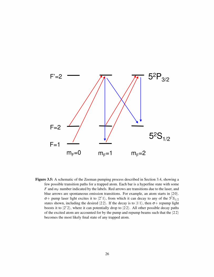
52P3/2
52S1/2
mF=0
F=1
F=2
F’=2
mF=1 m
F=2
Figure 3.5: A schematic of the Zeeman pumping process described in Section 3.4, showing afew possible transition paths for a trapped atom. Each bar is a hyperfine state with someF and mF number indicated by the labels. Red arrows are transitions due to the laser, andblue arrows are spontaneous emission transitions. For example, an atom starts in |2 0〉.σ+ pump laser light excites it to |2′ 1〉, from which it can decay to any of the 52S1/2states shown, including the desired |2 2〉. If the decay is to |1 1〉, then σ+ repump lightboosts it to |2′ 2〉, where it can potentially drop to |2 2〉. All other possible decay pathsof the excited atom are accounted for by the pump and repump beams such that the |2 2〉becomes the most likely final state of any trapped atom.
26

Chapter 4
The Miniature Atom Trap (MAT)
Our magneto-optical/magnetic trapping system is built, as previously stated, to laser cool and trap
either 87Rb or 85Rb. It can be seen in cartoon form in Fig. 4.1, and in labelled photographic form
in Fig. 4.2. Many of the details of the system have been thoroughly described in Fagnan’s thesis
and other works; these details will be summarized very briefly here. For further details, please see
[12, 13, 19].
4.1 Vacuum SystemThe average pressure in the system at any given time of experiment taking is 10−7 to 10−10 Torr.
To maintain this pressure, three separate vacuum pumping systems are used: a Thermionics IP-011
ion pump, two (now one) Varian Turbo-V 70 turbomolecular pumps attached to a Varian SH-100
roughing pump, and a set of chemical getter pumps which relies on a chemical reaction between the
pump’s active material and the background atoms [13]. The three pumps work in tandem to keep
the pressure both low and consistent over time, though the ion pump is sometimes turned off during
experiments because pumping in the test region may distort pressure readings [13].
During the summer of 2009, one of the two Varian Turbo-V 70 pumps failed. From July 19th,
2009, to late November, the system ran on only the ion and getter pumps, and therefore had to be
tightly sealed. Only Rb-Rb measurements were made during this time, since the seal prevented
the injection of any other background gases. Starting in December, the turbo pump system was
reactivated with only one pump. The current readout on the ion pump (the current is to maintain
the electromagnetic field that performs the ionization and pumping) has climbed from below 1 µA
in July to nearly 80 µA in April 2010, leading to fears that the ion pump will soon fail. As of this
writing, this has yet to happen.
When performing loss rate measurements against background gases other than Rb, the gas injec-
tion system, see in Fig. 4.1 is used. A residual gas analyzer determines the pressure of gas entering
the system. As these systems were not used during the course of this project, they are noted here
27

Figure 4.1: A simplified schematic of the MAT magneto-optical/magnetic trap. Diagram from[13], courtesy of David Fagnan.
simply for completion.
4.2 Rubidium Injection SystemA commercially available electrically-activated rubidium source (Alvatec As-2-Rb-25-V 2mm 25mg
source) is used to re-supply Rb to the vacuum chamber. Because the ion and getter pumps remove
Rb from the system over time, re-supply must be performed periodically to maintain enough Rb
for acceptable MOT fluorescence signal and signal-to-noise ratio. Refill procedure involves slowly
increasing the current to the source up to 5.0 A using a Sorensen DLM40-15 power supply, and
leaving the current at that value for 1 to 5 minutes before ramping the current back down. The time
during which the current is at 5.0 A determines roughly how much Rb is injected into the system.
The amount of Rb injected into the system cannot be controlled like those of the other background
gases.
Once loading is complete the Rb number density takes approximately 12-14 hours to equilibriate
[13]. During equilibration, the number density falls exponentially from some initial level to its final
28
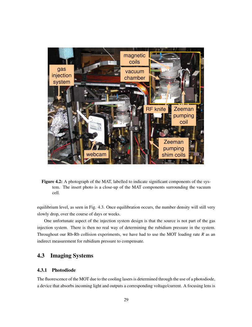
webcam
gas
injection
system
Zeeman
pumping
shim coils
Zeeman
pumping
coil
magnetic
coils
RF knife
vacuum
chamber
Figure 4.2: A photograph of the MAT, labelled to indicate significant components of the sys-tem. The insert photo is a close-up of the MAT components surrounding the vacuumcell.
equilibrium level, as seen in Fig. 4.3. Once equilibration occurs, the number density will still very
slowly drop, over the course of days or weeks.
One unfortunate aspect of the injection system design is that the source is not part of the gas
injection system. There is then no real way of determining the rubidium pressure in the system.
Throughout our Rb-Rb collision experiments, we have had to use the MOT loading rate R as an
indirect measurement for rubidium pressure to compensate.
4.3 Imaging Systems
4.3.1 Photodiode
The fluorescence of the MOT due to the cooling lasers is determined through the use of a photodiode,
a device that absorbs incoming light and outputs a corresponding voltage/current. A focusing lens is
29

0.0E+00
5.0E+06
1.0E+07
1.5E+07
2.0E+07
2.5E+07
3.0E+07
3.5E+07
4.0E+07
4.5E+07
5.0E+07
0 100 200 300 400 500 600
Time (min)
R (
s-1
)
Figure 4.3: An example of an Rb equilibration curve. MOT loading rate R is used as a proxyfor Rb background number density. An exponential decay has been fitted to the data,indicating that R decreases exponentially from a t = 0 value of (8.15±0.11)×107 s−1 toa steady state value of (9.249±0.084)×106 s−1.
placed in front of the cell in order to focus MOT fluorescence onto the photodiode aperture. Fagnan
gives the relationship between power from the light passing through the lens to MOT fluorescence
as
P≈ 0.92hνr2
lens
d2lens
NRscatter (4.1)
where Rscatter is the scatter rate of photons off of a trapped atom, and N is the total number of trapped
atoms, which is linear to P. Practically, this conversion is used to determine the initial loading rate
of atoms into the MOT, R, in units of number of atoms per second. It is worthwhile to note the
alignment of the photodiode that maximizes both signal and signal-to-noise ratio is dependent on
the exact position of the MOT trapped ensemble, and Eq. 4.1 does not include this effect. In
practice, at the start of any given experiment the photodiode is realigned to maximize signal and
30

signal-to-noise ratio.
4.3.2 CCD Camera
Instead of giving a power value, the CCD camera measures intensity, and therefore has two-dimensional
resolution. This is important to our experiments largely in that we use our FLI-MX0053307 CCD
camera to properly align the MOT. We are not concerned with the exact shape of the MOT ensemble,
only that it remains consistent over the course of an experiment, and does not rapidly change shape
or develop non-spherical patterns. The CCD was also used by Fagnan to determine the temperature
of the MOT trapped ensemble through absorptive imaging, yielding a value of 40-100 µK [13].
4.3.3 Webcam
We have recently installed a DLink DCS920 colour webcam to supplement the CCD camera. Other
than giving us a slightly different axis by which to view the atoms, and the ability to view the MOT
in real time, the camera can be viewed remotely. The webcam is part of a larger project to control
the entire MAT remotely, with a variety of applications from classroom demonstrations to remote
monitoring of experimental progress.
4.4 Laser SystemsThe lasers used to generate the pump and repump beams are external cavity diode lasers, whose
wavelengths are controlled by changing the orientation of the cavity grating and the laser injection
current. When the lasers are locked to a particular wavelength, the grating and current are electron-
ically controlled to compensate for any wavelength drift. A set of injection-locked slave lasers are
used to amplify the laser light before it reaches the MOT system. On the MAT table, the pump laser
provides 20 mW of power, while the repump laser provides 0.8 mW of power.
When we trap 87Rb in our MOT, the cooling laser is red-detuned 12 MHz from the 52S1/2
|F = 2〉 to 52P3/2 |F ′ = 3〉 transition. The repump beam is set to the transition 52S1/2 |F = 1〉 to
52P3/2 |F ′ = 2〉. When we trap 85Rb in our MOT, the cooling laser is red-detuned 12 MHz from the
52S1/2 |F = 3〉 to 52P3/2 |F ′ = 4〉 transition. The repump beam is set to the transition 52S1/2 |F = 2〉to 52P3/2 |F ′ = 3〉. Refer to [19] for more details.
Red-detuning is determined by a set of acoustic optical modulators (AOMs). As stated above,
we typically shift the cooling/trapping beam by 12 MHz. During magnetic trap loadings, we typi-
cally shift the beam to 40 MHz in order to obtain a colder distribution of atoms [13].
Light activation/deactivation is also achieved through the AOMs. A set of solenoid-powered
shutters prevents stray light from entering the system. These shutters have operation times generally
less than 20 ms, but within this regime they are sometimes quite variable [13].
31

4.5 The Magnetic CoilsOur set of magnetic quadrupole coils is composed of two identical water-cooled copper coils situ-
ated above and below our MOT. The exact technical specifications can be found in Djuricanin [12].
The coils have an 3µ0DR2
(D2+R2)5/2 (in accordance with Eq. 3.8) value of 55.7 G cm−1 A−1, and have been
tested up to 30 A. In practice, no more than 14 A has been used for experiments, due to even small
changes in coil temperature having an effect on the trap shape and number of atoms trapped.
In general, we run a 0.5 A (27.8 G cm−1 along the z-axis, or 13.9 G cm−1 along the x) current
through our coils to supply the Zeeman splitting necessary for the MOT.
4.6 The RF KnifeThe RF knife is a coil of 10 turns of copper wire 2.2 cm in diameter attached to the base of the MAT
glass vacuum chamber, as seen in Fig. 4.2. It is connected to a digital frequency synthesizer and
amplifier (that also controls our AOMs), which outputs a specific user-defined frequency. The RF
knife is electronically controlled via a UTBus computer driver through a LabView/Python command
console.
The RF knife has an effective frequency range of approximately 2 MHz to around 120 MHz
(see Fig. 4.4). Below 1 MHz and above 120 MHz, the amplitude of the RF knife output drops
considerably, and should no longer be considered effective. The Nyquist sampling frequency for
the frequency synthesizer is 150 MHz, and therefore it is impossible for the RF knife to operate at a
frequency higher than this value.
The RF knife drives hyperfine transitions at exactly one potential energy in the trap. During
experimentation, we commonly sweep the RF knife over a range of frequencies, in order to eliminate
all atoms of a certain energy or higher. The RF knife must be able to reach all values of potential
energy in the trap, and because 120 MHz is the upper RF frequency limit, this forces us to use the
RF knife only with traps of around 5 mK or less.
An atom with total energy E will explore the regions of the trap where the potential V < E. It is
then theoretically possible that setting the RF knife to a single frequency will eliminate all atoms of
a corresponding total energy or higher given enough time. (This is also the reason why we cannot
perform RF “surgery”, where all atoms of a narrow band of energy ∆E are removed from the trap.)
The amount of time this takes has not yet been determined, but testing whether setting a constant
RF frequency is an effective method of eliminating all atoms of a specific energy or higher should
be considered for future work.
The effectiveness over time of the RF knife was determined experimentally. Over the course
of 125 ms, all atoms in a 3.12±0.84 mK trap were eliminated by an RF knife sweep from 0 to 90
MHz. 125 ms has become the standard sweep time for all RF knife measurements.
Because RF sweeping eliminates all atoms from the trap of some energy or higher, RF sweeping
32

-60
-50
-40
-30
-20
-10
0
0 20 40 60 80 100 120 140
RF Frequency (MHz)
RF
Am
pli
tud
e (
dB
)
Figure 4.4: A plot of RF amplitude as a function of RF frequency νRF . The amplitude remainsrelatively constant except in the region of 0 - 2 MHz and past 115 - 120 MHz.
continuously is an effective way of setting the trap depth of a magnetic trap. This has been done
with considerable success, and the RF was used to set the trap depth for all heating measurements
in Section 6.2 and Section 6.3. It was not used to set the trap depth for any experiment that also
used Zeeman pumping; I describe the reason for this in Section 6.5.
4.7 The Zeeman-Optical Pumping SystemThe Zeeman-optical pumping system uses the same lasers as the MOT. Beam-splitting cubes are
used to siphon off a small amount of laser light from the pump and repump lasers. The Zeeman
pump beam must couple, per the description in Section 3.4, |F = 2〉 to |F ′ = 2〉; because of this
the Zeeman pump beam has a separate AOM from the MOT pump beam (which couples |F = 2〉 to|F = 3〉). Both the +1 and -1 orders of this AOM are used, one for 87Rb and one for 85Rb, to allow
for rapid switching of Zeeman pumping lasers for different isotopes. The Zeeman repump beam
does not require a separate AOM from the MOT repump, since both beams couple to the same
33
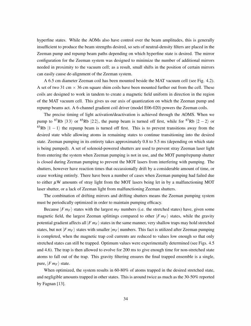
hyperfine states. While the AOMs also have control over the beam amplitudes, this is generally
insufficient to produce the beam strengths desired, so sets of neutral-density filters are placed in the
Zeeman pump and repump beam paths depending on which hyperfine state is desired. The mirror
configuration for the Zeeman system was designed to minimize the number of additional mirrors
needed in proximity to the vacuum cell; as a result, small shifts in the position of certain mirrors
can easily cause de-alignment of the Zeeman system.
A 6.5 cm diameter Zeeman coil has been mounted beside the MAT vacuum cell (see Fig. 4.2).
A set of two 31 cm × 36 cm square shim coils have been mounted further out from the cell. These
coils are designed to work in tandem to create a magnetic field uniform in direction in the region
of the MAT vacuum cell. This gives us our axis of quantization on which the Zeeman pump and
repump beams act. A 6-channel gradient coil driver (model E06-020) powers the Zeeman coils.
The precise timing of light activation/deactivation is achieved through the AOMS. When we
pump to 87Rb |3 3〉 or 85Rb |2 2〉, the pump beam is turned off first, while for 87Rb |2 −2〉 or85Rb |1 −1〉 the repump beam is turned off first. This is to prevent transitions away from the
desired state while allowing atoms in remaining states to continue transitioning into the desired
state. Zeeman pumping in its entirety takes approximately 0.8 to 5.5 ms (depending on which state
is being pumped). A set of solenoid-powered shutters are used to prevent stray Zeeman laser light
from entering the system when Zeeman pumping is not in use, and the MOT pump/repump shutter
is closed during Zeeman pumping to prevent the MOT lasers from interfering with pumping. The
shutters, however have reaction times that occassionally drift by a considerable amount of time, or
cease working entirely. There have been a number of cases when Zeeman pumping had failed due
to either µW amounts of stray light from the MOT lasers being let in by a malfunctioning MOT
laser shutter, or a lack of Zeeman light from malfunctioning Zeeman shutters.
The combination of drifting mirrors and drifting shutters means the Zeeman pumping system
must be periodically optimized in order to maintain pumping efficacy.
Because |F mF〉 states with the largest mF numbers (i.e. the stretched states) have, given some
magnetic field, the largest Zeeman splittings compared to other |F mF〉 states, while the gravity
potential gradient affects all |F mF〉 states in the same manner, very shallow traps may hold stretched
states, but not |F mF〉 states with smaller |mF | numbers. This fact is utilized after Zeeman pumping
is completed, when the magnetic trap coil currents are reduced to values low enough so that only
stretched states can still be trapped. Optimum values were experimentally determined (see Figs. 4.5
and 4.6). The trap is then allowed to evolve for 200 ms to give enough time for non-stretched state
atoms to fall out of the trap. This gravity filtering ensures the final trapped ensemble is a single,
pure, |F mF〉 state.
When optimized, the system results in 60-80% of atoms trapped in the desired stretched state,
and negligible amounts trapped in other states. This is around twice as much as the 30-50% reported
by Fagnan [13].
34
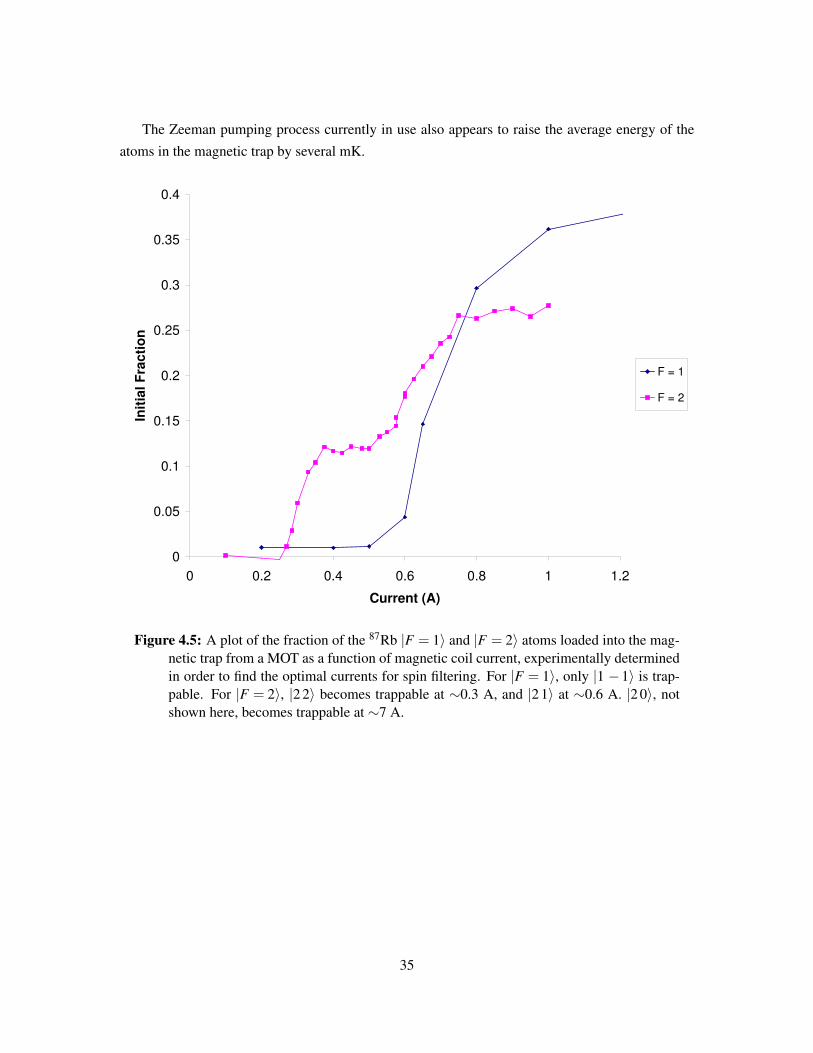
The Zeeman pumping process currently in use also appears to raise the average energy of the
atoms in the magnetic trap by several mK.
0
0.05
0.1
0.15
0.2
0.25
0.3
0.35
0.4
0 0.2 0.4 0.6 0.8 1 1.2
Current (A)
Init
ial
Fra
cti
on
F = 1
F = 2
Figure 4.5: A plot of the fraction of the 87Rb |F = 1〉 and |F = 2〉 atoms loaded into the mag-netic trap from a MOT as a function of magnetic coil current, experimentally determinedin order to find the optimal currents for spin filtering. For |F = 1〉, only |1 −1〉 is trap-pable. For |F = 2〉, |2 2〉 becomes trappable at ∼0.3 A, and |2 1〉 at ∼0.6 A. |2 0〉, notshown here, becomes trappable at ∼7 A.
35

0
0.1
0.2
0.3
0.4
0.5
0.6
0 0.2 0.4 0.6 0.8 1 1.2 1.4 1.6
Current (A)
Init
ial
Fra
cti
on
F = 3
F = 2
Figure 4.6: A plot of the fraction of the 85Rb |F = 3〉 and |F = 2〉 atoms loaded into the mag-netic trap from a MOT as a function of magnetic coil current, experimentally determinedin order to find the optimal currents for spin filtering. For |F = 3〉, |3 3〉 is trappable at∼0.2 A, |3 2〉 at ∼0.4 A, |3 1〉 at ∼0.85 A, and |3 0〉 (not shown) at ∼4.5 A. For |F = 2〉,|2 −2〉 becomes trappable at ∼0.3 A, and |2 −1〉 at ∼0.85 A. No data exists for |2 0〉,theoretically estimated to be trappable at currents past ∼7 A.
36

Chapter 5
Numerical Methods and Results
A number of numerical simulators were used during the tenure of my project. One is incomplete at
the time of this writing, and the other two were mostly complete before the start of my project. I
shall therefore describe each method in brief only.
5.1 Loss Cross-Section CalculatorThe loss cross-section calculator, written in FORTRAN77 by David Fagnan, calculates the total
and loss cross-section of atoms in a trap due to elastic collisions with background atoms [13]. The
code utilizes the theoretical machinery outlined in Chapter 2 to calculate | f (k,θ)|2, which it uses to
determine the loss cross-section σ . The code first finds the value of the coefficients of the Bessel
and Neumann functions that asymptotically describe a scattered wavefunction via the logarithmic
derivative method outlined by B.R. Johnson [23]. It then converts these values to T-matrix values,
which it then uses to calculate the scattering amplitude and total cross-section σtotal via Eqs. 2.34
and 2.35 [13]. Finally, it uses Gauss-Legendre integration of Eq. 2.12 to determine the total loss
cross-section σ , and Boltzmann averages the total and loss cross-sections to determine 〈σtotalv〉 and〈σv〉 [13].
Fagnan’s original code was utilized and optimized to calculate scattering between trapped Rb
and background Ar (to produce the theoretical curve in Fig. 1.1). Aside from changing the atomic
mass of the background scatterer and modifying the C6 and C12 interaction values, modifying the
code to determine Rb-Rb collisional cross-sections required increasing the number of partial waves
used in the calculation by a factor of approximately four for any given velocity. The code was used
to determine an Rb-Rb 〈σv〉 versus trap depth curve (Fig. 1.2), used in the thesis for analyzing the
hyperfine dependence data 1.
1Note that the Rb-Rb interaction potential is independent of the isotopes being used in our experiment. The differencein 87Rb-87Rb, 87Rb-85Rb and 85Rb-85Rb 〈σv〉 is solely due to the mass the collision constituents, making this difference1 - 2% of 〈σv〉 at best. All Rb-Rb 〈σv〉 cited in this thesis are for 87Rb-87Rb.
37

The code has also been modified to perform a number of different calculations, including calcu-
lating velocity-averaged heating rates due to elastic background collisions (Eq. 2.20), or a velocity
averaged differential cross-section⟨ dσ
dΩ
⟩.
5.2 Magnetic Trap Simulator
5.2.1 Overview of the Simulator
At the outset of this project, it was believed that a direct simulation of the atoms in the trap would be
the most viable method of investigating heating. A simulator would additionally be able to replicate
some of the more complex details of our trap, such as the exact shape of the potential well and
Majorana losses. The code, written in Python, is nearing completion.
The simulation begins by creating an ensemble of trapped atoms. These atoms have kinetic
energies determined from a Maxwell-Boltzmann distribution, and are distributed in space according
to a user-defined function (a Gaussian is currently being used). The simulation then uses the velocity
verlet method to simulate how the atoms evolve in the trap over time. The trapped atoms are
periodically subjected to collisions, in accordance with the rate of collisions from a background
gas of a certain number density and a Maxwell-Boltzmann velocity distribution. The code derives
the momentum imparted to the trapped atom in the collision from differential cross-sections. The
incident direction of the background particle is assumed to be random, and therefore this momentum
is given a random direction and added to the momentum of the trapped particle. This negates the
problem (mentioned in Section 2.1.1) of Eq. 2.4 becoming invalid for collisions in which the trapped
atom already has significant kinetic energy. Since collisions are treated individually, the simulator
also allows us to determine the loss and heating rates in trapped ensembles with a distribution of
energies.
Because of how time-consuming calculating cross-sections is, differential cross-section values
at various angles and k-values were calculated using a heavily-modified version of the loss cross-
section calculator. The simulator runs a two-dimensional spline across these values in order to
determine dσ
dΩfor any θ and k.
5.2.2 Changes in the Scattering Amplitude due to Varying the C12 Coefficient
The C12 value for Rb-Ar collisions was calculated (instead of determined from literature) from the
C6 value (280 atomic units) and assuming a 50 cm−1 well - this gave 8.603× 10⁷ a.u. The same
calculation method was initially used for Rb-Rb collisions, giving 2.154×10¹⁰ a.u. (C6 = 4430 a.u.,
from Bali et al.) for the Rb-Rb C12 value, used to create Fig 1.2 [3]. Patil and Tang give a C12 value
of 1.19×10¹⁰, which is the C12 value eventually used to calculate differential cross-sections for the
simulator [27]. It is the case, however, that the loss and total cross-sections of Rb-Rb collisions are
38

constant to within an 11% deviation over a wide range of C12 values, from 102 to 1010 (see Fig.
5.1). The same is true for Rb-Ar collisions, which is why it was set somewhat arbitrarily when
calculating Rb-Ar 〈σv〉 with respect to trap depth.
What does change when C12 is varied is the shape of the differential cross-section as a function
of θ , as seen in Fig. 5.2. At C12 values of less than 109 a.u., there are significant high frequency
oscillations in the differential cross-section across all values of θ . Starting at values of 109, the
differential cross-section at high values of θ begin to “smooth out”, and by 1012 the differential
cross-section curve appears largely free of oscillations except at angles smaller than θ =∼ 0.02.
These changes to the differential cross-section eventually impact the total cross-section, but this
occurs only past 5× 10¹⁰. We believe that the oscillations at low values of C12 are due to the
inclusion of large numbers of partial waves to allow for convergence of the cross-section values
[18]. As the C12 value becomes larger, the potential becomes more and more repulsive, which may
lead to the changes seen in Fig. 5.2. Why exactly these changes occur when C12 passes 109 are
not entirely clear from my investigation. Because both the loss cross-section calculator and the
simulator output aggregate loss rates, we need only worry about total and loss collisional cross-
sections. I have thus chosen a value of C12 = 1.19× 10¹⁰, in accordance with Patil and Tang, for
the simulator calculations. It may be, however, that the difference in differential cross-section due
to varying C12 value is worth investigation in the future.
5.3 Multi-Channel Loss Cross-Section CalculatorThe multi-channel loss cross-section calculator, written in FORTRAN90 by Zhiying Li, calculates
the total and loss cross-section of trapped atoms due to collisions with background atoms taking
into consideration the hyperfine states of the collision constituents. For the calculations performed
for this thesis, the code considers a trapped 87Rb or 85Rb ensemble composed of a single hyperfine
state (ex. |3 3〉) experiencing collisions with a background gas composed of 87Rb and 85Rb. The dis-
tribution of 87Rb and 85Rb |F mF〉 states is assumed to be uniform, meaning incoming background
atoms have an equal probability of being in any ground state |F mF〉. It includes the contributions
to 〈σv〉 of various hyperfine state changing inelastic collisions, as well as changes to 〈σv〉 due to
the whether the combined spin state of the collision constituents is a triplet or a singlet.
The assumption of a uniform distribution of |F mF〉 states for the background gas means that
the contribution to 〈σv〉 from the identical particle phenomenon detailed in Section 2.5 would be
invariant to changes in trapped ensemble |F mF〉 state. The effect is also small, as identical con-
stituent collisions represent only a small fraction of all collisions: numerical calculations using a
modified version of the loss cross-section calculator indicate that the effect is on the order of 5% of〈σv〉. For these reasons, changes in 〈σv〉 due to identical particle collisions were not included in
the calculations.
The resulting calculations verified our 〈σv〉 calculations: the multichannel 〈σv〉 deviated only
39

0
500
1000
1500
2000
2500
3000
3500
1.00E+00 1.00E+03 1.00E+06 1.00E+09 1.00E+12 1.00E+15
C12 (a.u.)
σ (
Å2 )
σ(total)
σ(loss)
Figure 5.1: A semilog plot of numerically determined σ (loss cross-section) and σtotal , forcollisions between trapped Rb and background Rb travelling at 293 m/s, as functions ofC12 value. σ is calculated for a 1 K trap. The value of both σ (loss cross-section) andσtotal are constant to within ∼ 10% until C12 ≥∼ 5×10¹⁰ atomic units.
by several percent from the 〈σv〉 calculated by Fagnan’s loss cross-section calculator [21]. The
deviation is smaller than the one-sigma error bars reported in our experimental data (Fig. 1.2).
40

1.0E+00
1.0E+01
1.0E+02
1.0E+03
1.0E+04
1.0E+05
1.0E+06
1.0E+07
1.0E+08
0 0.5 1 1.5 2 2.5 3 3.5
Angle (rads)
|f(k
,θ)|
2 (Å
2 /rad
s)
1.00E+07
1.00E+10
1.00E+12
Figure 5.2: A semilog plot of numerically determined | f (k,θ)|2 as a function of θ for col-lisions between trapped Rb and background Rb travelling at 293 m/s. Each curve wascalculated using a different C12, noted in the legend in atomic units. As C12 value in-creases, the number of oscillations seen in the | f (k,θ)|2 curve decreases.
41

Chapter 6
Procedure and Experimental Results
6.1 General ProcedureOur standard method of discerning properties of our magneto-optical trap is by taking a MOT load-
ing curve. This is done by starting with a steady-state MOT ensemble, turning off the magnetic field
for 500 ms to eject the ensemble, and then turning the field back on and letting the trap load once
again. This trap loading follows Eq. 3.1, and therefore fitting an exponential decay to the curve
allows us to determine the loss rate 〈Γtotal〉. Fitting a straight line to the section of the loading curve
just after the magnetic coils turn back on allows us to estimate the initial MOT loading rate, R. Fig.
6.1 is an example of a MOT loading curve.
The magnetic trap does not use the lasers, and this means we cannot continuously determine
the number of trapped atoms via laser fluorescence as we do with the MOT. Instead, we begin
with a steady state MOT, further cool the atoms, and then turn off the lasers while simultaneously
ramping up the magnetic field gradient from 27.8 G cm−1 along the z-axis to the final desired value
(typically around 278.5 G cm−1 along the z-axis) in 7.5 ms. If Zeeman pumping is used, it is
performed immediately before ramping up the magnetic field gradient. The pumping itself takes 0.8
ms, while the gravity filtering takes 200 ms. Once this is complete, the trap is left to evolve on its
own for some designated time. At the end of this time, the magnetic field is ramped back down over
15 ms 1, and the lasers are flashed back on, taking a measurement of the ensemble fluorescence,
before the magnetic fields are turned off to empty the trap. The magnetic fields are then turned on
after 500 ms of wait time, creating a MOT loading curve from which we can determine the initial
loading rate R.
From this procedure, a single point along the magnetic trap loss curve is determined (see Fig.
6.2). Unlike the loading curves of Fig. 6.1, loss curves values are normalized to the steady state
1This is not enough time for atoms to move across the length of the trap, which is why procedures like RF knifing andZeeman pumping require more than 100 ms of wait time to ensure all atoms are lost from the trap
42

MOT value, and therefore represent the fraction of atoms from the original MOT ensemble that
were successfully loaded into the magnetic trap and have not been lost over a certain magnetic trap
hold time (henceforth referred to as “trapped fraction”). A number of loss-determination curves
must then be produced in order to fill out the magnetic trap loss curve.
Rb-Rb collisions were the dominant collisions in our trap for all experiments described in this
section.
0
0.2
0.4
0.6
0.8
1
1.2
-2 0 2 4 6 8 10
Time (s)
Flu
ore
sc
en
ce
(V
)
(1)
(2)
(3)
Empty MOT Fluorescence
Full MOT Fluorescence
Figure 6.1: An example of a MOT loading curve. The curve is produced by (1) starting witha steady-state MOT ensemble, (2) turning off the magnetic field for 500 ms to eject theensemble, and then (3) turning the field back on and letting the trap load once again. Thefluorescence seen by the photodiode is not zero when there is no trapped ensemble at (2)because some laser light still scatters off the MAT vacuum cell. The resulting curve is anexponential rise from the zero-level at (2) to the MOT steady state fluorescence.
43

0
0.2
0.4
0.6
0.8
1
1.2
1.4
-5 0 5 10 15 20 25
Time (s)
Flu
ore
scen
ce (
V)
(1)
(2)
(3)
(4)
Figure 6.2: An example of a series of magnetic trap loss-determination curves. Each curve(taking the orange curve as our example) begin with a steady state MOT (1). We thencool the atoms, and turn off the lasers while simultaneously ramping up the magneticfield gradient in 7.5 ms. If Zeeman pumping is used, it is performed immediately afterthat for 200 ms. Once this is complete, the trap is left to evolve on its own (2) forsome designated time (during which the lasers are off, so no fluorescence reaches thephotodiode). At the end of this time, the magnetic field is ramped back down over 15 ms,the lasers are flashed back on, taking a measurement of the ensemble fluorescence (3),before the magnetic fields are turned off to empty the trap. The magnetic fields are thenturned on, creating a MOT loading curve (4). Each of these loss-determination curvesdetermines a single value on a magnetic trap loss curve (the multicoloured diamonds oneach curve), which can be strung together to create an exponential decay. Note that theMOT steady state value appears to increase over time - this is possibly due to heating ofthe magnetic coils. Because we normalize point (3) to the MOT steady state fluorescenceto produce a trapped fraction, small amounts of deviation such as seen in this graph canbe neglected.
44

6.2 Measurement of Trap Energy DistributionThe first attempt at deducing the rate of heating in the trap was to measure directly how many atoms
of certain energies were being trapped. Sweeping the RF knife from some lower frequency ν to an
upper frequency corresponding to an energy above the trap depth eliminates all trapped atoms with
energies larger than E(x) (to use terminology defined in Section 3.3). Therefore, varying the lower
frequency of this sweep allows us to explore the energy distribution within the trap. Because each
RF knife sweep will eliminate all atoms above a certain energy, only one point in the distribution
can be determined per experimental run, it takes many identical runs to fully map out a trap energy
distribution.
We performed a number of experiments using 87Rb |1 −1〉 where a magnetic trap was held for
a certain amount of time, and then the energy distribution of that trap was determined. 87Rb |1 −1〉was chosen so that no consideration of the effect Bouyer et al. noted, of low RF efficacy due to
having to transition trapped atoms across multiple trappable |F mF〉 states, was needed [6]. The
trap depth was chosen to be 3.14± 0.84 mK for the experiments so that for every Rb-Rb trap loss
collision, there was also one Rb-Rb heating collision, per Eq. 2.19 and Fig. 1.2.
An example of our results is Fig. 6.3. This curve is similar to the metastable He ensemble
energy distribution (in a Ioffe-Pritchard trap) found by Browaeys et al. using their RF knife [7].
If heating were evident in the trap, the energy distribution determined would have shifted with
increasing hold time toward a distribution with higher average energy. Our experiments showed,
however, this is not the case, as can clearly be seen in Fig. 6.3. Believing it may be possible that the
system was in a sort of steady state where shifts in the energy distribution are not apparent, we then
modified the experimental procedure so that at the start of the magnetic trap hold, we used an RF
sweep to eliminate the more energetic half of the trapped atoms. The result was an apparent increase
in shot noise in the system, but over long periods of time there was still no discernable heating of
the atoms (Fig. 6.4). For Fig. 6.3, the total number of trapped atoms had decreased by more than
35% over 8000 ms due to elastic collisions that do result in immediate trap loss, indicating that the
other 50% of the trapped atoms have undergone an average of 0.7 heating collisions over the same
amount of time. The fact that no change is seen may indicate that the majority of these collisions
impart extremely small amounts of energy to the trapped ensemble.
It was eventually deemed, after multiple negative results using this method, that we needed to
switch to a method that is aggregate, to more easily distinguish small amounts of heating.
6.3 Measurement of Heated FractionA “heated fraction” measurement is an aggregate method of determining the heating rate within
a magnetic trap. At the beginning of the magnetic trap hold, all atoms of energy Emid or higher
in the trap are eliminated using an RF sweep with lower frequency limit ν for 125 ms. The trap
45

0
0.1
0.2
0.3
0.4
0.5
0.6
0.7
0.8
0.9
1
0 5 10 15 20 25
Trapped Atom Energy Upper Limit (MHz)
Fra
cti
on
of
Tra
pp
ed
Ato
ms
500 ms
1000 ms
4000 ms
8000 ms
Figure 6.3: Cumulative energy distribution curves of an 87Rb |1 −1〉 3.14± 0.84 mK mag-netic trap at various hold times (denoted in the legend), determined by 125 ms RF sweepsat varying lower frequencies. Each data point on a distribution curve indicates the frac-tion of atoms trapped with some particular energy (in MHz) or lower (at some time).Over 8000 ms, the total number of trapped atoms decreased by more than 33% (eachcurve is normalized to the total number of atoms in the trap at the time to eliminate traploss biases), but no discernable heating is seen.
is then allowed to evolve over some time; during this time, the RF knife can be used to set the
trap depth. At the end of this hold time, the RF knife is again swept with lower limit ν for 125
ms, eliminating any atoms that might have been heated past Emid during the hold time. This gives
trapped fraction measurement FW (t). A second experimental run with an identical initial procedure
is then performed, but at the end no RF knife is used, giving us FO(t), the trapped fraction that
includes all trapped atoms regardless of energy. The heated fraction is defined as
FH(t) = 1− FW (t)FO(t)
. (6.1)
46

0
0.1
0.2
0.3
0.4
0.5
0.6
0.7
0.8
0.9
1
0 5 10 15 20 25
Trapped Atom Energy Upper Limit (MHz)
Fra
cti
on
of
Tra
pp
ed
Ato
ms
500 ms
1000 ms
4000 ms
8000 ms
Figure 6.4: Cumulative energy distribution curves of an 87Rb |1 −1〉 3.14± 0.84 mK mag-netic trap at various hold times (denoted in the legend), determined by 125 ms RF sweepsat varying lower frequencies. The RF knife was also used to eliminate all atoms of en-ergy 8 MHz or above at the beginning of each trap hold. Each data point on a distributioncurve indicates the fraction of atoms trapped with some particular energy (in MHz) orlower (at some time). Over 8000 ms, the total number of trapped atoms decreased bymore than 20% (each curve is normalized to the total number of atoms in the trap atthe time to eliminate trap loss biases). This lower loss rate may be because the averageenergy of the trapped atoms is lower and therefore more incoming collisions result inheating rather than trap loss, but due to the significant increase in noise in the distribu-tions it is not possible to determine if any heating has actually occured.
Because initially the RF knife sets FW = FO, this value can be understood as the fraction of atoms
that have migrated from the 0 - Emid energy bin to the Emid - trap depth U0 energy bin due to heating
collisions. Therefore, a very crude estimate of the energy E of the trapped ensemble is
E ≈ NFH(t)U0 +Emid
2+
NEmid
2(1−FH(t))
47

= N(U0
2FH(t)+
Emid
2), (6.2)
where N is the number of atoms in the trap. If we want the heating rate per atom, i.e. the average
energy 〈E〉 imparted to a single trapped atom per second, we take the derivative with respect to time
and divide by N:
d 〈E〉dt≈ U0
2dFH
dt, (6.3)
Initial attempts at determining heated fraction over time gave us plots such as Fig. 6.5, which
showed two surprising features. The first was that the initial FH value did not appear to be zero,
even though the RF knife was supposed to have eliminated all atoms from the high energy bin. It
was initially believed the existence of the non-zero initial heated fraction was because the RF knife
was inadvertently heating the rest of the trapped atoms. Heated fraction experiments where the trap
depth was not set using the RF knife, however, showed the same non-zero initial FH . The second
was that there was a significant amount of noise when taking the measurements, which suggested
that the average of many sets of heated fraction data was needed.
6.3.1 Relationship Between Heated Fraction and Trap Depth
We attempted to determine the relation between FH and trap depth. This was determined by taking
FH measurements, as detailed above, for a number of different trap depths all set using the RF knife.
For the experiment, Emid was set to 13.9± 1.1 MHz (0.667± 0.053 mK), and an initial RF sweep
was used to eliminate all atoms of energy 13.9 MHz or lower for each data run. Each FH curve
was built out of data from five different experimental runs: five sets of FW and FO were taken for
each point on each FH curve. From this set, 25 values of FH are determined. From these 25 values,
both the FH average and an estimate of the shot noise one-sigma error can be found. The resulting
FH curves are plotted in Fig. 6.6. These curves were analyzed with linear best fits on Gnuplot; the
results are given in Table 6.1 and plotted in Figs. 6.7 and 6.9.
Let us assume that our trapped ensemble starts with negligible energy (untrue in our traps).
From Eq. 2.17, nBg 〈qv〉 is a crude first estimate of the rate of heating collisions in the trap, where
q is defined in Eq. 2.18. nBg 〈qv〉 for a trap of depth Emid , which we designate nBg 〈qv〉m, would be
a crude estimate for the rate of collisions that do not impart enough energy into the trapped atoms
to elevate them above Emid and be counted as part of the heated fraction. nBg 〈qv〉 - nBg 〈qv〉m would
then be a crude measure for the heated fraction rate. We plot the heated fraction rate versus 〈qv〉 -〈qv〉m in Fig. 6.8.
48

0
0.05
0.1
0.15
0.2
0.25
0.3
0.35
0.4
0 5 10 15 20 25
Hold Time (s)
Heate
d F
racti
on
Figure 6.5: Plot of FH vs. magnetic trap hold time for 87Rb |1 −1〉 in a 1.3± 0.14 mK trap.Magnetic coil gradient was set to 5 A, but the 1.3 mK trap depth was set by a continuousRF sweep from 27.53 MHz to 90 MHz over the magnetic trap hold time. An initialRF sweep was used to eliminate all atoms of energy 7.96± 0.87 MHz (0.382± 0.042mK) or lower. The error shown is derived from best fitting for the trapped fraction,and is not a measure of the shot noise of the points. A linear best fit performed onGnuplot, plotted here in magenta, gave an initial fraction of 0.1473±0.0077, and a slopeof 0.0073± 0.0012 s−1. Using Eq. 6.3, this gives us a heating rate per atom of ∼0.2MHz s−1, or ∼9 µK s−1.
Table 6.1: Table of Gnuplot fit results for the FH curves in Fig. 6.6.
Trap Depth (MHz) FH Slope (s−1) FH(t = 0) d 〈E〉/dt (MHz s−1) d 〈E〉/dt (µK s−1)19.8±1.6 0.0032±0.0010 0.0679±0.0082 0.031±0.010 1.50±0.4929.5±2.3 0.00370±0.00095 0.1127±0.0093 0.054±0.014 2.62±0.6739.1±3.1 0.0058±0.0014 0.115±0.014 0.113±0.027 5.4±1.357.9±4.6 0.0069±0.00078 0.1296±0.0085 0.200±0.022 9.6±1.1
49

0
0.05
0.1
0.15
0.2
0.25
0.3
0.35
0 5 10 15 20
Time (sec)
He
ate
d F
rac
tio
n
20 MHz
29 MHz
39 MHz
57 MHz
Figure 6.6: Plot of FH vs. magnetic trap hold time for 87Rb |1 −1〉 curves for traps of varyingdepth. Magnetic coil gradient was set to 7 A, but the trap depth was set by a continuousRF sweeps. The four depths used were 19.8±1.6 MHz (0.949±0.074 mK), 29.5±2.3MHz (1.41±0.11 mK), 39.1±3.1 MHz (1.88±0.15 mK) and 57.9±4.6 MHz (2.78±0.22 mK). Emid was set to 13.9±1.1 MHz (0.667±0.053 mK). Error bars for 19.8 and57.9 MHz FH curves are included to give a visual example of the level of shot noise inthe system.
50

0
0.001
0.002
0.003
0.004
0.005
0.006
0.007
0.008
0.009
0 10 20 30 40 50 60 70
Trap Depth (MHz)
He
ate
d F
rac
tio
n R
ate
(s
-1)
Figure 6.7: Plot of Fig. 6.6 FH best fit slopes vs. trap depth.
51

0
0.001
0.002
0.003
0.004
0.005
0.006
0.007
0.008
0.009
0 0.3 0.6 0.9 1.2 1.5
<qv> - <qv>m (10-9
cm3 s
-1)
He
ate
d F
rac
tio
n R
ate
(s
-1)
Figure 6.8: Plot of Fig. 6.6 FH best fit slopes vs. 〈qv〉 - 〈qv〉m. To determine 〈qv〉 and 〈qv〉m,the estimate 〈qv〉 = 〈σtotalv〉 - 〈σv〉 was used. Theoretically, the relationship betweenthe two values is, to first order, linear, and the slope is nBg. A linear best fit to thedata was performed in Gnuplot, and is plotted alongside the data. The fit’s slope is4.07±0.75×106 cm−3 and intercept is 0.00141±0.00073 s−1.
52

0
0.02
0.04
0.06
0.08
0.1
0.12
0.14
0.16
0 10 20 30 40 50 60 70
Trap Depth (MHz)
Init
ial
He
ate
d F
rac
tio
n
Figure 6.9: Plot of Fig. 6.6 FH initial value (best fit y-intercept) vs. trap depth.
53
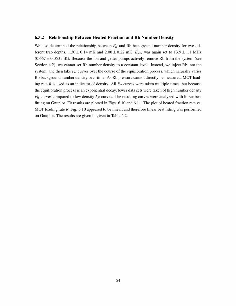
6.3.2 Relationship Between Heated Fraction and Rb Number Density
We also determined the relationship between FH and Rb background number density for two dif-
ferent trap depths, 1.30± 0.14 mK and 2.00± 0.22 mK. Emid was again set to 13.9± 1.1 MHz
(0.667± 0.053 mK). Because the ion and getter pumps actively remove Rb from the system (see
Section 4.2), we cannot set Rb number density to a constant level. Instead, we inject Rb into the
system, and then take FH curves over the course of the equilibration process, which naturally varies
Rb background number density over time. As Rb pressure cannot directly be measured, MOT load-
ing rate R is used as an indicator of density. All FH curves were taken multiple times, but because
the equilibration process is an exponential decay, fewer data sets were taken of high number density
FH curves compared to low density FH curves. The resulting curves were analyzed with linear best
fitting on Gnuplot. Fit results are plotted in Figs. 6.10 and 6.11. The plot of heated fraction rate vs.
MOT loading rate R, Fig. 6.10 appeared to be linear, and therefore linear best fitting was performed
on Gnuplot. The results are given in given in Table 6.2.
54

0
0.01
0.02
0.03
0.04
0.05
0.06
0.07
0.08
0.00E+00 1.00E+07 2.00E+07 3.00E+07 4.00E+07 5.00E+07
R (s-1
)
He
ate
d F
rac
tio
n R
ate
(s
-1)
1.3 mK
2 mK
Figure 6.10: Plot of the relationship between FH rate and MOT loading rate R for a 1.30±0.14mK trap and 2.00± 0.22 mK trap (set using continuous RF knife sweeps with lowerfrequencies 27.53 and 42.72 MHz, respectively). Emid was set to 0.667± 0.053 mK.These data points were determined by performing Gnuplot best fits on FH curves takenover a number of R values.
55

0
0.02
0.04
0.06
0.08
0.1
0.12
0.14
0.00E+00 1.00E+07 2.00E+07 3.00E+07 4.00E+07 5.00E+07
R (s-1
)
Init
ial
He
ate
d F
rac
tio
n
1.3 mK
2 mK
Figure 6.11: Plot of the relationship between FH(t = 0) initial fraction and MOT loading rateR for a 1.30± 0.14 mK trap and 2.00± 0.22 mK trap (set using continuous RF knifesweeps with lower frequencies 27.53 and 42.72 MHz, respectively). Emid was set to0.667±0.053 mK. These data points were determined by performing Gnuplot best fitson FH curves taken over a number of R values.
56

Table 6.2: Table of Gnuplot fit results for the relationship between FH rate (denoted F ′H) andMOT loading rate R, for Fig. 6.10. The leftmost 2 mK point was not used in the best fit ofthe 2 mK data. The relationship between d 〈E〉/dt (denoted 〈E ′〉) and MOT loading rateR is also given for each trap in accordance with Eq. 6.4.
Trap Depth (mK) dF ′H/dR ×10−7 F ′H(R = 0) d 〈E ′〉/dR (µK s−2)1.30±0.14 0.0086±0.0013 −0.00035±0.00080 5.60±1.12.00±0.22 0.01183±0.00095 0.0071±0.0013 11.8±1.6
The best fit slopes on Fig 6.10 can be converted to a measure of how d 〈E〉/dt = E ′ changes
with R:
E ′ =d 〈E ′〉
dRR. (6.4)
6.4 Measurement of Pure State Loss Rate vs. Rb PressureWith the Zeeman pumping system, we could determine loss rates without having to consider the
ambiguity of trapping multiple |F mF〉 states in a single magnetic trap. Initial loss rate comparisons
taken in December gave the loss rate of 85Rb |3 3〉 as 5.4 times greater than |2 −2〉 (in a magnetic
trap of the same trap depth), and the loss rate of 87Rb|1 −1〉 as 1.4 times greater than |2 2〉 [5].
We elected to create experimental plots of loss rates of 85Rb |3 3〉 and |2 −2〉, and 87Rb |2 2〉 and|1 −1〉, against R, the MOT loading rate 2. Because R is linearly proportional to the not-measurable
Rb background density (Eq. 3.2), the slope of a Γ vs. R plot would be proportional to 〈σv〉, which
multi-channel collisions have shown is independent of hyperfine state [21].
Magnetic trap loss curves at varying values of R were taken at trap depth, for all states, of ∼2.8
mK. R was varied by injecting Rb into the system and utilizing the equilibration process to reduce
Rb number density in the system over time. The 85Rb rates were measured in February, while the87Rb was measured in March. The result was a linear relationship (as expected) between Γ and R
for all hyperfine states. These plots were all analyzed with linear best fits in Gnuplot. The results
are graphed in Figs. 6.12 and 6.13, and best fit values are in Table 6.3.
6.5 Anomalous ResultsWhile data was being taken, two anomalous results were observed. The first is a slight decrease
in loss rates in state 87Rb |1 −1〉 when Zeeman pumping is being used compared to when Zeeman
pumping is not used (only |1 −1〉 is trappable for 87Rb |F = 1〉). This decrease seems to vary
between days, and can be anywhere from less than 10% up to 30%. It does not seem to vary
2Because one of the turbomolecular pumps had failed, the only background gas that was available at the time was Rb,and once the pump system was restored, the use of Rb had already been decided.
57

Table 6.3: Table of Gnuplot linear best fit results for data plotted in Figs. 6.12 and 6.13. Withinerror, the slopes of both states match for both 85Rb and 87Rb, as predicted by numericalcalculation.
Hyperfine State dΓ/dR Γ(R = 0)85Rb |3 3〉 0.01975±0.00052 0.0773±0.0040
85Rb |2 −2〉 0.02061±0.00042 0.0036±0.002887Rb |2 2〉 0.04763±0.00089 0.0163±0.0016
87Rb |1 −1〉 0.04686±0.00040 0.02021±0.00058
monotonically with trap depth. While energy distribution experiments have shown that Zeeman
pumping imparts additional energy into the trap, a hotter ensemble should be lost more quickly and
not more slowly. It is unknown if the same effect occurs for other trappable hyperfine states: 87Rb|1 −1〉 is the only state where only one |F mF〉 state is trapped regardless of whether or not Zeeman
pumping is used, and so no other states could be tested. Zeeman pumping was used for all states in
the measurements of Γ vs. R in section Section 6.4, and so the results from that section presumably
are not affected by this phenomenon.
The second is a rapid initial loss of atoms that occurs over the span of approximately two seconds
whenever the RF knife and Zeeman pumping are used in tandem (and not seen within noise when
only the RF knife or Zeeman pumping is in use). This loss was initially seen in 85Rb, and it was
assumed to be due to the atoms having to undergo multiple RF transitions before entering into an
untrappable |F mF〉 state. It, however, can also be observed for 87Rb |1 −1〉, as seen in Fig. 6.14.
The rate and degree of initial loss varies with current, but the long-term losses are not affected.
Attempts were made at subtracting the long-term decay curve from the experimental data, and
fitting the resulting clean short-term losses with exponential decays in order to determine the loss
rate ΓRIL of these curves. The noise in the subtracted data is high, and the determined ΓRILs did not
within error show any dependence on current (see Fig. 6.15).
58

0
0.1
0.2
0.3
0.4
0.5
0.6
0.00E+00 5.00E+07 1.00E+08 1.50E+08 2.00E+08 2.50E+08
R (s-1
)
Lo
ss
Ra
te Γ
(s
-1)
|2 -2>
|3 3>
Figure 6.12: Plot of total loss rate Γ vs. MOT loading rate R for 85Rb |3 3〉 and |2 −2〉 inmagnetic traps. Trapping current was set to 2.2 A (a 2.83±0.77 mK trap) for |3 3〉, and3.4 A (a 2.83± 0.74 mK trap) for |2 −2〉. The RF knife was not used. While thereis a y-intercept (Γ(R = 0)) difference between the two lines, their slopes are identical,within error. Linear best fits determined using Gnuplot have been plotted alongsideexperimental data.
59

0
0.02
0.04
0.06
0.08
0.1
0.12
0.14
0.16
0.18
0.2
0.00E+00 1.00E+07 2.00E+07 3.00E+07 4.00E+07
R (s-1
)
Lo
ss
Ra
te Γ
(s
-1)
|2 2>
|1 -1>
Figure 6.13: Plot of total loss rate Γ vs. MOT loading rate R for 87Rb |2 2〉 and |1 −1〉 inmagnetic traps. Trapping current was set to 4.53 A (a 2.83±0.74 mK trap) for |1 −1〉,and 2.2 A (a 2.83±0.77 mK trap) for |2 2〉. The RF knife was not used. While there issmall a y-intercept (Γ(R = 0)) difference between the two lines, their slopes are identi-cal, within error. Linear best fits determined using Gnuplot have been plotted alongsideexperimental data.
60

0.01
0.1
1
0 2.5 5 7.5 10
Time (s)
Fra
cti
on
Tra
pp
ed
1.815 A no RF
2.5 A RF
5 A RF
7.5 A RF
10 A RF
12 A RF
Figure 6.14: An investigation into rapid intial losses from an 87Rb |1 −1〉 magnetic trap. Thetrap depth is kept either at 1.00±0.15 mK using the magnetic coils alone at 1.815 A, orat 1 mK using a combination of an RF sweep from 21.0944 MHz to 100 MHz and themagnetic coils at currents 2.5 A or higher. Long-term losses look identical, but a rapidinitial loss can be seen for high-currents. Note that at 12 A the trapped fraction reducesto just a few percent in under 2 seconds - this does not occur in an identical trap (usingRF sweeping to hold the trap depth) where Zeeman pumping is not used!
61
-1
0
1
2
3
4
5
6
7
8
9
0 0.05 0.1 0.15 0.2 0.25 0.3 0.35 0.4 0.45
1/Current (A-1
)
Lo
ss
Ra
te Γ
RIL
(s
-1)
Figure 6.15: A plot of ΓRIL, obtained by fitting exponential decays to the fast initial losses, asa function of A−1 (instead of A; see Section 7.3). Unfortunately, the resulting data isambiguous, but does seem to suggest no dependence of ΓRIL on A−1.
62

Chapter 7
Discussion
7.1 Measurement of Heated FractionThe measurements of heating presented in Section 6.3 are internally consistent. For example, the
ratio of best fit slopes presented in Table 6.2, 1.4, is consistent, within error, with how heated fraction
rate increases with trap depth, seen in Fig. 6.7. They are also consistent, qualitatively, with the
theory presented in Chapter 2. We expect that the heated fraction rate dFH/dt should increase with
trap depth, since an increase in trap depth is equivalent to an increase in θmin, which would result in
more collisions being heating collisions. Heated fraction rate should also scale with background Rb
pressure, as the rate at which Rb-Rb collisions occur is linearly proportional to background Rb.
The crude estimates of d 〈E〉/dt indicate that we are in the regime of several µK of heating
per second. Of course, as we do not know the Rb pressure in the system, we cannot know if this
value truly makes sense compared to other magnetic traps. We are currently investigating various
methods to determine Rb background number density.
The fact that FH(t = 0) 6= 0 is not easily explainable. It appears to scale with trap depth, but its
relation to Rb pressure is, by Fig. 6.11, either significantly more complicated or nonexistent. If it
is nonexistent, then FH(t = 0) 6= 0 would appear to be a phenomenon related to the trapped atoms
rather than background collisions. It is possible the RF knife is not entirely effective in clearing out
atoms in 125 ms. Very recent experiments with RF knife sweeping suggest that sweeping from 0
- 100 MHz (which was done to determine the 125 ms interval) may be more effective at clearing
atoms than sweeping from 10 - 100 MHz or 20 - 100 MHz. If, however, initial heated fraction does
increase with Rb pressure (the left half of Fig. 6.11 could be interpreted in this way), it may be due
to low-angle collisions moving a small group of atoms just past Ecut . It is important to note that in
our measurements the trap is allowed to evolve for a small amount of time before measurements are
taken, which may be enough time for these low-angle collisions to shift the energy distribution in
the trap.
63

Unfortunately, heated fraction is a value that has a very complex dependency to the various
parameters we set in the trap. It depends on how (at what frequency) the initial cut of energetic
atoms is performed, the trap depth of the magnetic trap, and, most importantly, the distribution of
energies possessed by the trapped atoms at any given time. It is therefore prohibitive to attempt an
analytical derivation of the various dependencies of heated fraction.
Rb-Rb collisions were chosen as the heating collisions to be investigated in our trap. This
is because the quantum diffractive turn-off of the Rb-Rb 〈σv〉 vs. trap depth plot occurs near 1
mK, easily accessible by our magnetic traps and RF knife, which allows us to create traps where
a substantial number of collision are heating collisions. The Rb-Ar turn-off is near 10 mK, which
is barely reachable by the magnetic coils and unreachable by the RF knife. It may be prudent,
however, for future heating work to include experimenting with Rb-Ar collisions not only because
results with a second type of collision can support the theory of heating presented in this thesis, but
also because it is possible to measure Ar background number density.
The most important next step to studying heated fraction is the creation of the numerical mag-
netic trap simulator detailed in Section 5.2. As stated earlier, heated fraction is a value that has
a very complex dependencies to trap parameters, and this is also true of the relationship between
heated fraction and the exact d 〈E〉/dt for the magnetic trap, which is ultimately what is desired
when measuring trap heating. For this reason, the most effective method of corroborating experi-
mentally determined heated fraction with the elastic scattering theory presented in Chapter 2 is to
simulate the evolution of trap energy over time.
7.2 Measurement of Pure State Loss Rate vs. Rb PressureFrom Table 6.3, we can definitively say that the 〈σv〉 of 85Rb |3 3〉 and |2 −2〉 are the same, within
error. The 〈σv〉 of 87Rb |2 2〉 and |1 −1〉 are also the same within error. The differences in loss
rates can be explained by a difference in the values of Γ(R = 0). The initial measurements using
Zeeman pumping taken in December are somewhat consistent with this picture. The December data
was taken at low R values (corresponding to low Rb background number density), and the ratio
of Γ(R = 0) |3 3〉 and |2 −2〉 is 21.5, meaning that a factor of 5 difference is easily accomodated.
This is not the case for 87Rb: the ratio of Γ(R = 0) |2 2〉 and |1 −1〉 is 1.24, and 1.4 is larger than
the one-sigma error for this ratio. It could simply be experimental error, but it is also possible that
Γ(R = 0) has changed over time.
We cannot easily compare between isotopes; loading rate R is state-specific, whereas Rb-Rb〈σv〉 is between the trapped ensemble and all background Rb. The Rb source for the MOT produces
the natural abundance isotope ratio of 2.5932±0.0020 85Rb for every 87Rb, which suggests that for
any trap depth the slope of Γ vs. R for 87Rb should be 2.59 times larger than for 85Rb [1]. From our
data, the ratio is 2.341±0.046, close to, but not within error of, 2.5932±0.0020.
While we have experimentally verified our theory on calculating 〈σv〉, the difference in the
64

intercept, Γ(R = 0), remains a mystery. Archival Rb-Ar Γ vs. nAr data also shows (although not
as definitively, since Zeeman pumping had yet to be installed) that while 〈σv〉 does not change
regardless of the hyperfine state being trapped, there are intercept differences. If it is the case that
there is a hyperfine dependence for 〈σv〉 of elastic collisions between trapped Rb and some other
background constituent M, the difference in intercept between any two hyperfine states should vary
with trap depth, and a plot of this variance should follow the 〈σv〉 vs. trap depth curve of Rb-M
collisions. Alternatively, the reason for the y-intercept difference may be a hitherto unconsidered
loss mechanism.
As an aside, it is notable that a Γ vs. R plot could be used to determine the Rb background num-
ber density in the system, provided we trust our numerical calculations (Fig. 1.2) and experimental
data. Since the slope of such a graph is α 〈σv〉, where α is some coefficient, and we theoretically
know 〈σv〉, the conversion between R and number density should be α . For a trap at 2.83 mK, the
Rb-Rb 〈σv〉 is 2.9279× 10⁻⁹ cm3 s−1. Using this value to convert the x-axis for Figs. 6.12 and
6.13, we obtain Figs. 7.1 and 7.2
0
0.1
0.2
0.3
0.4
0.5
0.6
0.00E+00 5.00E+07 1.00E+08 1.50E+08 2.00E+08
nRb (cm-3
)
Lo
ss
Ra
te Γ
(s
-1)
|2 -2>
|3 3>
Figure 7.1: Fig. 6.12 with the x-axis rescaled (α = 0.6893) from MOT loading rate R to Rbbackground number density.
65

0
0.02
0.04
0.06
0.08
0.1
0.12
0.14
0.16
0.18
0.2
0.00E+00 1.00E+07 2.00E+07 3.00E+07 4.00E+07 5.00E+07 6.00E+07
nRb (cm-3
)
Lo
ss
Ra
te Γ
(s
-1)
|2 2>
|1 -1>
Figure 7.2: Fig. 6.13 with the x-axis rescaled (α = 1.6138) from MOT loading rate R to Rbbackground number density.
66

7.3 Anomalous ResultsOne possibility for the anomalous results is Majorana losses. If this is the case, then Eq. 3.11
suggests that the loss rate should scale as the inverse of magnetic gradient. In our trap, this is
equivalent to the inverse of current. As mentioned in Section 6.5, we fitted exponential decays
to the fast initial losses seen in Fig. 6.14. We then plotted the loss rates from the exponential
decays, ΓRIL, versus A−1. The results are ambiguous, as can be seen in Fig. 6.15. One problem
with the Majorana loss explanation is that it should be seen when no Zeeman pumping is used. In
fact, it should be more prominent, since Zeeman pumping is known to impart additional energy
into the trap, would make it less likely for trapped atoms to explore the region near the magnetic
zero. Experimental results have shown this is not the case, and these rapid initial losses are only
prominent when the RF knife and Zeeman pumping operate in tandem.
Another potential explanation is that the Zeeman pumping system excites atoms to energies too
high for the RF knife to initially reach. These energetic atoms will eventually (over 1 - 2 seconds)
explore the trap and cross a position at which the RF knife can affect them. This is likely the case
for 12 A traps, since the trap depth is actually higher than the effective upper limit of the RF knife
at around 120 MHz. This cannot be the case, however, for 5 A traps, which can be cleaned in their
entirety by the RF knife, and still exhibit rapid initial losses. In these cases, we hypothesize that the
Zeeman pumping system can impart kinetic energy to atoms close to the centre of the trap. Atoms
with enough energy to reach a potential where the RF knife induces transitions may not reach such
potentials until it explores the trap for some time. More thorough testing is needed to determine if
this hypothesis is indeed correct.
7.4 ConclusionWe investigated low scattering angle elastic collisions that change the trapped ensemble energy
distribution without resulting in immediate trap loss, or “heating collisions”, and the dependence
of elastic collisional loss cross-sections on the hyperfine state of the trapped rubidium ensemble,
in our MAT magnetic trap. Our results show that the average rate of energy imparted to a trapped
atom in our system is on the order of 1 µK per second. We also show that the Rb-Rb loss rate slope〈σv〉 is invariant of hyperfine state, indicating that any loss dependency on hyperfine state rests with
collisions with other species, or other forms of loss.
67

Chapter 8
Appendix
8.1 List of Data Files UsedThe files that contain the data used in this thesis are listed below, for future reference.
• Figs. 1.1, 1.2 - CollisionThesis.xls
• Fig. 4.4 - RF Efficacy Thesis.xls
• Figs. 4.5, 4.6 - 6-25-09 F12 Init Thesis.xls and 10-16-09 F23 Init Thesis.xls
• Figs. 5.1, 5.2 - DCS Thesis.xls
• Figs. 6.3, 6.4 - 12-1-09 RF Data Thesis.xls
• Fig. 6.5 - 1-20-21-2010 Data Thesis.xls
• Table 6.1, Figs. 6.6, 6.7, 6.8, 6.9 - 3-11-10 Data Thesis.xls
• Table 6.2, Figs. 6.10, 6.11 - 3-25-10 Data Thesis.xls
• Table 6.3, Figs. 6.12, 6.13, 7.1, 7.2 - 2-24-25 Data Thesis.xls, 3-18-10 Data Thesis.xls
• Figs. 6.14, 6.15 - 3-10-10 Data Thesis.xls
68

Bibliography
[1] CRC Handbook of Chemistry and Physics, 90th ed., 2010. Internet Version. → pages 64
[2] M. Anderson, J. Ensher, M. Matthews, C. Wieman, and E. Cornell. Observation ofBose-Einstein Condensation in a Dilute Atomic Vapor. Science, 269(3), 1995. → pages 2
[3] S. Bali, K. O’Hara, M. Gehm, S. Granade, and J. Thomas. Quantum-diffractive backgroundgas collisions in atom-trap heating and loss. Phys. Rev. A, 60(1), 1999. → pages 9, 11, 12, 38
[4] H. Beijerinck. Rigorous calculation of heating in alkali-metal traps by background gascollisions. Phys. Rev. A, 61(033606), 2000. → pages 11, 12
[5] J. Booth. Zeeman Pumping - Results from Dec. 5, 2009. Technical report, University ofBritish Columbia, 2009. → pages 57
[6] P. Bouyer, V. Boyer, S. Murdoch, G. Delannoy, Y. le Coq, A. Aspect, and M. Lecrivain.RF-induced evaporative cooling and BEC in a high magnetic field. In Bose-EinsteinCondensates and Atom Lasers. 2000. → pages viii, 22, 23, 24, 45
[7] A. Browaeys, A. Robert, J. Sirjean, S. Poupard, D. Nowak, D. Boiron, C. Westbrook, andA. Aspect. Thermalization of magnetically trapped metastable helium. Phys. Rev. A, 64(034703), 2001. → pages 1, 45
[8] J. P. Burke. Theoretical Investigation of Cold Alkali Atoms. PhD thesis, University ofColorado, 1999. → pages 15
[9] E. Charron, M. Cirone, A. Negretti, J. Schmiedmayer, and T. Calarco. Theoretical analysis ofthe implementation of a quantum phase gate with neutral atoms on atom chips. Phys. Rev. A,74(012308), 2006. → pages 2
[10] M. Child. Molecular Collision Theory. Dover Publications, Inc., Mineola, New York, 1974.→ pages 6, 12
[11] B. Desruelle, V. Boyer, S. Murdoch, G. Delannoy, P. Bouyer, and A. Aspect. Interruptedevaporative cooling of 87Rb atoms trapped in a high magnetic field. Phys. Rev. A, 60(3),1999. → pages 22
[12] P. Djuricanin. Magnetic Coil: Assembly and Instruction Manual. Technical report,University of British Columbia, 2009. → pages 27, 32
69

[13] D. Fagnan. Study of Collision Cross Section of Ultra-Cold Rubidium using a Magneto-Opticand pure Magnetic Trap, 2009. Undergraduate thesis, University of British Columbia. →pages viii, 1, 3, 7, 12, 16, 17, 18, 20, 22, 27, 28, 31, 34, 37
[14] D. Fagnan, J. Wang, C. Zhu, P. Djuricanin, B. Klappauf, J. Booth, and K. Madison.Observation of quantum diffractive collisions using shallow atomic traps. Phys. Rev. A, 80(022712), 2009. → pages 2, 3, 6, 13
[15] R. Folman, P. Kruger, J. Schmiedmayer, J. Denschlag, and C. Henkel. Microscopic AtomOptics: From Wires to an Atom Chip. Adv. At., Mol., Opt. Phys., 48, 2002. → pages 2
[16] D. J. Griffiths. Introduction to Quantum Mechanics. Pearson Prentice Hall, Upper SaddleRiver, New Jersey, 2nd edition, 2005. → pages 12, 13, 14, 19, 22
[17] B. Klappauf. zeeman module.py, 2009. Python code. → pages viii, 21
[18] R. Krems. Re: C12 Value for Rb-Rb, 2010. Private communications (e-mail), March 16. →pages 39
[19] K. Ladouceur. Experimental Advances Toward a Compact Dual-Species Laser CoolingApparatus. Master’s thesis, University of British Columbia, 2008. → pages 27, 31
[20] Z. Li. New mechanisms for external field control of microscopic interactions in ultracoldgases. PhD thesis, University of British Columbia, 2009. → pages 15
[21] Z. Li. Trap loss rates for 85Rb cold gases, 2010. QDG/Theory Group Meeting, February 25th.→ pages 40, 57
[22] R. Long, T. Steinmetz, P. Hommelhoff, W. Hansel, T. Hansch, and J. Reichel. MagneticMicrochip Traps and Single-Atom Detection. Phil. Trans. R. Soc. Lond. A, 361, 2003. →pages 2
[23] N. Markovic. Notes on Scattering Theory. Chalmers University of Technology, 2003. →pages 12, 13, 14, 15, 37
[24] H. J. Metcalf and P. van der Straten. Laser Cooling and Trapping. Spring-Verlag, New York,New York, 1999. → pages 1, 16, 17
[25] T. P. Meyrath. Experiments with Bose-Einstein Condensation in an Optical Box. PhD thesis,University of Texas at Austin, 2005. → pages 22
[26] NIST. Fundamental Physical Constants from NIST, 2006. Available online athttp://physics.nist.gov/cuu/Constants/index.html. → pages vi, 6
[27] S. Patil and K. Tang. Multipolar polarizabilities and two- and three-body dispersioncoefficients for alkali isoelectronic sequences. J. Chem. Phys., 106(6), 1997. → pages 38
[28] D. A. Steck. Rubidium 85 D Line Data (revision 2.1.1), 2009. Available online athttp://steck.us/alkalidata. → pages 19
70

[29] D. A. Steck. Rubidium 87 D Line Data (revision 2.1.1), 2009. Available online athttp://steck.us/alkalidata. → pages 19
[30] G. K. Woodgate. Elementary Atomic Structure. Oxford University Press, New York, NewYork, 2nd edition, 1983. → pages 19, 22
71