KEYWORDS:

urban planning, social sustainability, segregation,

neighborhood, agent-based simulation

ABSTRACT

Different social groups tend to settle in different parts of

cities leading over time to social segregation.

Neighborhood obviously plays an important role in this

process – and what constitutes neighborhood is a

cognitive notion. In segregation analysis neighborhood

borders are often drawn arbitrarily or simple

assumptions are used to weight neighbor influences.

Some authors have developed ideas to overcome such

approaches by more detailed models. In this work we

investigate the size of a cognitive neighborhood on the

base of a continuous, geographically unlimited

definition of neighborhood, using a distance-dependent

function as such neighborhood “size” definition. We use

agent-based simulation of the choice of residence as our

primary investigation tool. Tobler’s first law of

geography tells us that close things are more related

than far ones. Extrapolating this thought and applying it

to the question discussed here one could expect that

closer neighbors have – on their own and in sum – more

influence than those living further apart. The “sum” in

the last sentence would lead to a neighborhood

weighting of less than the inverse square of distance.

The results of this investigation confirm that this is the

case.

INTRODUCTION

The population of a city is not equally distributed, but

tends to segregate according to the different

characteristics of the inhabitants and the areas in the

city. That means different inhabitants tend to live in

different areas. Segregation plays an important role in

city planning and in many cases it is deemed negative.

Urban planners try to maintain a state of social

sustainability in urban areas, which in very short words

means that the mixture of different inhabitants should

not exceed certain threshold values. In particular,

planners try to avoid clusters of socially underprivileged

people because the real world has shown that such areas

evolve in a negative way in many respects, e.g. crime.

Cities are living and ever-changing entities. Most things

to be found in cities are the result of some kind of

human-driven process or processes. Urban planners try

to control these processes to some degree, but from

today’s point of view, these will probably never be fully

predictable. The work presented in this paper aims to

contribute towards a better understanding of segregation

as one important process in a city.

RESEARCH QUESTION

We assume that segregation in a city is the result of a

long-lasting process of choice of residence by the

inhabitants. Every place of residence exists within a

neighborhood (a collection of places with relevant

characteristics), and the neighborhood plays an

important role in the choice of residence. According to

Tobler’s first law of geography (Tobler 1970) close

things are more related than those that are far apart.

Accordingly, the far neighborhood should be less

important for the choice of residence than the one close

by. The question we ask here is how distance-dependent

this importance is. In other words we try to find a

distance-dependent function that allows us to

mathematically weight the distant neighborhood against

the one close by for the choice of residence.

STATE OF THE ART

Methods for the numerical measuring of segregation

from the 1950s are still significant today (Duncan &

Duncan 1955). The corresponding calculations are now

a standard procedure used by official statistics in many

countries. A next important step was the introduction of

entropy-based segregation indices in the 1970s (Theil

1972), which are used in this work.

A milestone in the explanation of the causes of

segregation was the work of Schelling in the 1970s

(Schelling, 1978), who used agent-based simulations.

He demonstrated that feedback effects can play a

significant role in segregation. The detection of these

effects is naturally difficult using static statistical

methods (non-dynamic, not regarding time lapse). Static

statistical methods for correlating segregation with other

factors are now standard tools in administrative practice.

INVESTIGATION OF COGNITIVE NEIGHBORHOODSIZE BY AGENT-

BASED SIMULATION Jens Steinhoefel

Frauke Anders

Dominik Kalisch

Hermann Koehler

Reinhard Koenig

Chair for Computer Science in Architecture

Bauhaus-University Weimar

Belvederer Allee 1, 99421 Weimar, Germany

E-mail: jens.steinhoefel, frauke.anders, dominik.kalisch, hermann.koehler, reinhard.koenig@uni-weimar.de

Proceedings 26th European Conference on Modelling andSimulation ©ECMS Klaus G. Troitzsch, Michael Möhring,Ulf Lotzmann (Editors)ISBN: 978-0-9564944-4-3 / ISBN: 978-0-9564944-5-0 (CD)

Researchers increasingly use simulations, see e.g.

Feitosa et. al. (2007) and Crooks (2010). In this paper

we follow the simulation approach of Schelling. Further

direct predecessors of this paper, who also

basic idea of Schelling, are Benenson (1998), Benenson

and Omer (2002) and the Circle City model in Koenig

(2010).

Geographic Information Systems (GIS), which allow

the provision of high-resolution digital data, are used on

a regular basis as a tool in segregation analysis today.

Until now, raster-based GIS/raster

simulation systems are used by researchers, for example

in Feitosa et. al. (2007), Laurie and Jaggi (2003),

and Waren (2005). Crooks (2010), however, proposed

the application of vector-based systems, which is the

method used in the present work.

Various authors have asked questions about the

influence of neighborhood size on the outcome

segregation models (Wasserman and Yohe 2001, Laurie

and Jaggi 2003, Crooks 2010). They have noted that an

increasing neighborhood size (more generally: an

increasing weight of far neighbors) results in stronger

segregation effects, like the value of a se

or the size of segregation cluster areas.

In Benenson & Omer (2002) the authors emphasize that

segregation measures are dependent o

unit (city, borough, district, block, etc.) used for their

calculation, and can differ significantly according

selected scale for the same data used

investigate the question of how large the environment

that people perceive as their neighborhood, which

would be best suited for the description of residential

segregation. Voronoi polygons are used to define

neighborhoods at various levels (level

neighbors, level 2: direct neighbors of the direct

neighbors, etc.). This discrete approach of neighborhood

definition is further developed in the present work to a

continuous approach.

RESEARCH APPROACH

Segregation is a time-dependent process and there are

many decision makers – the people who choose a

residence. Using agent-based simulation as an

investigation tool is therefore an obvious choice and

this respect we follow Schelling’s approach

thing about agent-based simulation is the simplicity

modeling it allows to explain complex phenomena.

These two levels we use here, too. The phenomenon we

try to explain is segregation. In the (agent

simulation model we need some kind of social

submodel for the inhabitants and an infrastructure

submodel for the environment they live in (the city)

along with status transition rules to run the simulation.

These rules involve the social and the infrastructure

submodel and need to incorporate the

distance-dependent weighting function. Using this

Researchers increasingly use simulations, see e.g.

et. al. (2007) and Crooks (2010). In this paper

ion approach of Schelling. Further

who also follow the

basic idea of Schelling, are Benenson (1998), Benenson

and Omer (2002) and the Circle City model in Koenig

Geographic Information Systems (GIS), which allow

resolution digital data, are used on

as a tool in segregation analysis today.

based GIS/raster-based spatial

simulation systems are used by researchers, for example

d Jaggi (2003), Fosset

and Waren (2005). Crooks (2010), however, proposed

based systems, which is the

Various authors have asked questions about the

influence of neighborhood size on the outcome of

segregation models (Wasserman and Yohe 2001, Laurie

and Jaggi 2003, Crooks 2010). They have noted that an

increasing neighborhood size (more generally: an

neighbors) results in stronger

segregation effects, like the value of a segregation index

& Omer (2002) the authors emphasize that

segregation measures are dependent on the settlement

unit (city, borough, district, block, etc.) used for their

ificantly according to the

used. They therefore

investigate the question of how large the environment is

as their neighborhood, which

would be best suited for the description of residential

segregation. Voronoi polygons are used to define

various levels (level 1: direct

neighbors, level 2: direct neighbors of the direct

discrete approach of neighborhood

definition is further developed in the present work to a

dependent process and there are

the people who choose a

based simulation as an

investigation tool is therefore an obvious choice and in

’s approach. The nice

based simulation is the simplicity of

modeling it allows to explain complex phenomena.

els we use here, too. The phenomenon we

try to explain is segregation. In the (agent-based)

simulation model we need some kind of social

submodel for the inhabitants and an infrastructure

submodel for the environment they live in (the city)

us transition rules to run the simulation.

These rules involve the social and the infrastructure

submodel and need to incorporate the aforementioned

dependent weighting function. Using this

simulation model we try to reproduce a given

segregation scenario by optimizing the weighting

function.

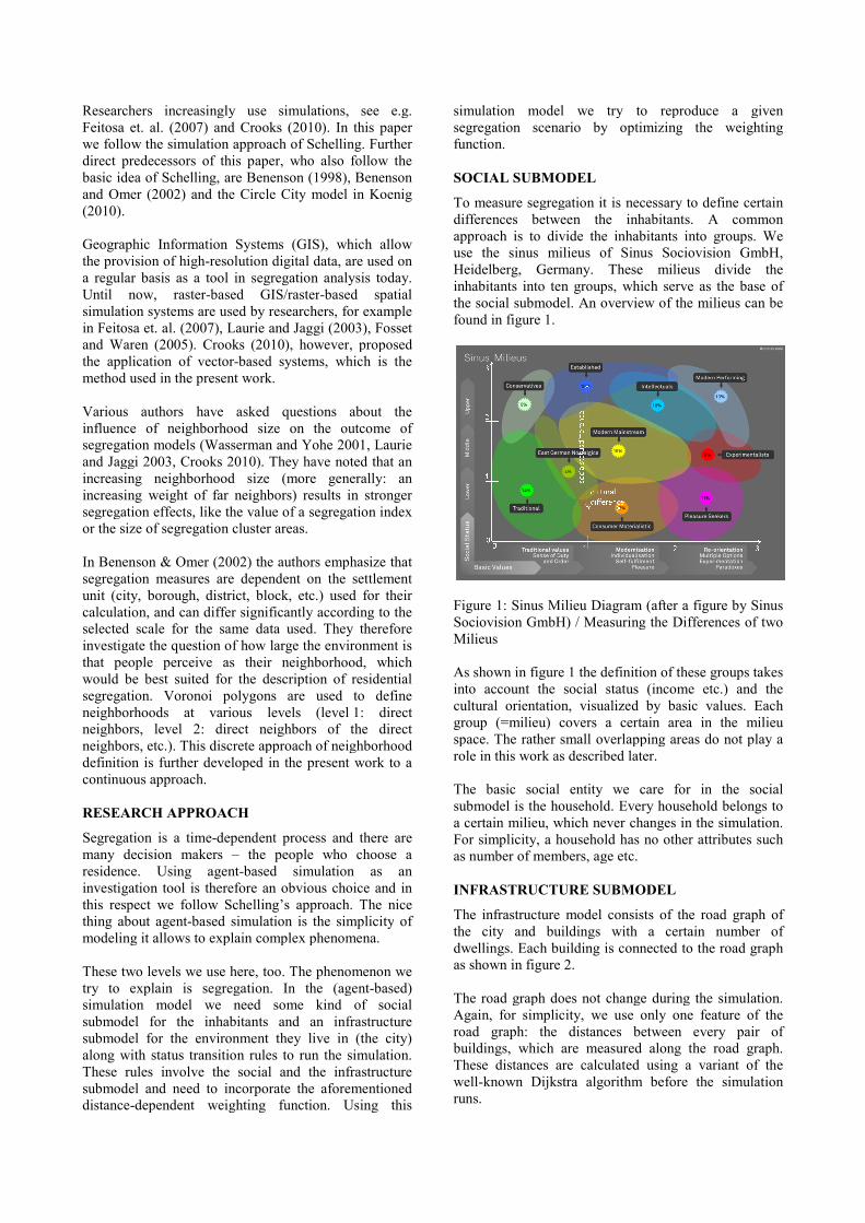
SOCIAL SUBMODEL

To measure segregation it is necessary to define certain

differences between the inhabitants. A common

approach is to divide the inhabitants into groups. We

use the sinus milieus of Sinus

Heidelberg, Germany. These milieus divide the

inhabitants into ten groups, which serve as the base of

the social submodel. An overview of the milieus can be

found in figure 1.

Figure 1: Sinus Milieu Diagram (after a figure

Sociovision GmbH) / Measuring the Differences of two

Milieus

As shown in figure 1 the definition of these groups takes

into account the social status (income etc.) and the

cultural orientation, visualized by basic values. Each

group (=milieu) covers a cer

space. The rather small overlapping areas do not play a

role in this work as described later.

The basic social entity we care for in the social

submodel is the household. Every household belongs to

a certain milieu, which never ch

For simplicity, a household has no other attributes

as number of members, age etc.

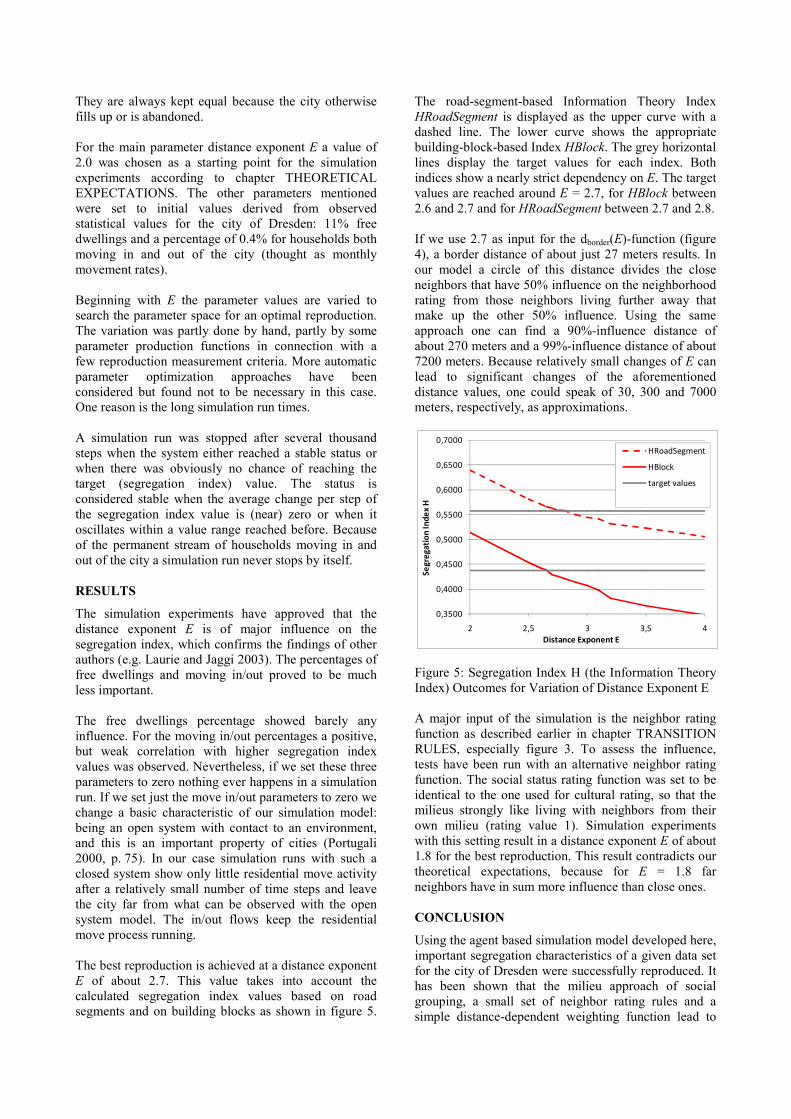
INFRASTRUCTURE SUBMODEL

The infrastructure model consists of the road graph of

the city and buildings with a certain number of

dwellings. Each building is connected to the road graph

as shown in figure 2.

The road graph does not change during the simulation.

Again, for simplicity, we use only one feature of the

road graph: the distances between every pair of

buildings, which are measured alo

These distances are calculated using a variant of the

well-known Dijkstra algorithm before the simulation

runs.

simulation model we try to reproduce a given

scenario by optimizing the weighting

To measure segregation it is necessary to define certain

differences between the inhabitants. A common

approach is to divide the inhabitants into groups. We

use the sinus milieus of Sinus Sociovision GmbH,

Heidelberg, Germany. These milieus divide the

inhabitants into ten groups, which serve as the base of

the social submodel. An overview of the milieus can be

Figure 1: Sinus Milieu Diagram (after a figure by Sinus

Sociovision GmbH) / Measuring the Differences of two

As shown in figure 1 the definition of these groups takes

into account the social status (income etc.) and the

cultural orientation, visualized by basic values. Each

group (=milieu) covers a certain area in the milieu

space. The rather small overlapping areas do not play a

role in this work as described later.

The basic social entity we care for in the social

submodel is the household. Every household belongs to

a certain milieu, which never changes in the simulation.

a household has no other attributes such

number of members, age etc.

INFRASTRUCTURE SUBMODEL

The infrastructure model consists of the road graph of

the city and buildings with a certain number of

ch building is connected to the road graph

The road graph does not change during the simulation.

Again, for simplicity, we use only one feature of the

road graph: the distances between every pair of

buildings, which are measured along the road graph.

These distances are calculated using a variant of the

known Dijkstra algorithm before the simulation

Figure 2: Infrastructure Model: Buildings connected to

the Road Graph of the City

TRANSITION RULES

The matter of this work is segregation, which is caused

by repeated choice of residence. Because the households

themselves don’t change during the simulation,

transition rules only need to determine the choices of

residence and nothing else.

As stated above (see RESEARCH QUESTION), in the

approach used here every choice of residence taken by a

household is based on the neighborhoods of the

potential new residence locations (free dwellings, not

occupied by a household). The neighborhood of a

dwelling is defined by all the neighbors of that dwelling,

and these are all households in the city. The rating of

each neighborhood is accordingly based on the ratings

of all neighbors.

To be of use for the choice of residence by a household

the neighbors need to be rated differently. The

phenomenon of segregation as observed in real cities

shows that this is the case and that people tend to live

with similar people more than they do with different

people.

The authors have developed a neighbor rating based on

the Sinus milieu diagram in a pragmatic way. This

rating is arbitrary and based on nothing else than

general rules which in the opinion of the authors feel

right and are plausible and, again, the criterion of

simplicity.

The general neighbor rating rules are as follows:

(R1) Regarding just the “Basic Values” (cultural axis)

of the milieu diagram (see figure 1 above), every

household wants to live with neighbors who are as close

as possible in the diagram.

(R2) Regarding just the social status axis every

household wants to live with neighbors slightly above

its own position in the milieu diagram.

To operationalize these rules, the neighbor rating is

again broken down into a cultural (neighbor) rating and

a social status (neighbor) rating. The milieu diagram

was overlaid with a coordinate system with coordinate

value ranges of [0..3] for each axis. The cultural and

social status differences between the milieus have been

measured using this coordinate system. To be able to

measure these differences every household needs to

have a position in the milieu diagram. In the given

segregation scenario, the milieu (group) of a household

is known, but not its position in the milieu diagram.

Therefore the position of the centroid of each milieu

area was used as the position of all the households

belonging to this milieu. Figure 1 illustrates the

statements of this paragraph.

The differences measured have to be turned into cultural

and social status rating values for a neighboring

household.

For the cultural rating the following function is used:

the rating value is 1 (the maximum) when the cultural

difference is 0, and the rating value is 0 (the minimum),

when the cultural difference is +3 or -3. For all other

cultural differences the values are interpolated

piecewise linear as shown in figure 3.

To apply the “slightly above” statement in neighbor

rating rule (R2), a different piecewise linear function is

used as social status rating. See figure 3. Notably the

maximum rating value of 1 is not reached at a social

status difference of 0, but for a small positive difference

(0.25).

Figure 3: Rating Functions for Cultural and Social

Status Differences

The rating value for a neighbor of a certain milieu is

calculated by adding the cultural and social status rating

values vectorially in a Cartesian coordinate system. The

value range of the neighbor rating is therefore [0..1].

Because there are 10 milieus and every milieu is rated

by every milieu, a 10 x 10 matrix of possible neighbor

rating values results.

To calculate a neighborhood rating, all the neighbor

ratings are incorporated into a weighted mean value.

0

0,5

1

-3 -2 -1 0 1 2 3

Ra

tin

g V

alu

e

Difference in the Milieu Diagram along accordant Axis

Cultural Rating Social Status Rating

The weight w is the inverse of distance d exponentiated

by a fixed exponent E:

1 Ew d= (F1).

The final neighborhood rating function is

1

E

nb

nbh E

r dr

d=∑∑

(F2)

over all neighbors with rnb as the rating for a single

neighbor.

The simulation is run in discrete time steps. The

neighborhood ratings for all dwellings are calculated

first and then stay fixed for that time step. The agents in

the simulation can act in the following ways:

(A1) A household leaves the city. This happens

spontaneous by a fixed leave probability.

(A2) A household tries to move to a free dwelling with

a better neighborhood rating. If one is available the

household moves. All free dwellings in the city are

considered.

(A3) New households try to move into the city. A new

household occupies the best dwelling it can get, if one is

available. If not, the household is withdrawn from the

simulation. The number of new households is

determined by a truncated Gaussian distributed

probability with fixed parameters (derived from an input

mean).

A number of parameters such as minimum

neighborhood rating of the current dwelling before

moving, minimum improvement of the neighborhood

rating of the potential new dwelling compared with the

current dwelling and others could be removed during

the development of the simulation in order to simplify it

without damaging the reproduction quality.

SEGREGATION SCENARIO REPRODUCTION

The segregation scenario reproduction quality is

measured using a segregation index. The Information

Theory Index H first published by Theil (1972) has been

chosen for this purpose. Other indices could have been

employed, but most of them are highly correlated

(Massay and Denton 1988), and this one has nice

properties. It is widely accepted, well investigated, has a

fixed value range of [0..1] and allows for the calculation

of a single segregation value for the whole city for any

number of groups.

Segregation index values are calculated for the given

segregation scenario (target value) and after every step

(including the final step) of a simulation run. The

reproduction is considered better the smaller the

difference to the target value is.

Because segregation indices are fairly dependent on the

base unit used for their calculation (Benenson and Omer

2002) we have chosen two quite different ones, the road

segment as a quasi one-dimensional base unit and the

building block (a couple of buildings surrounded but not

divided by a road) as a two-dimensional base unit.

USED DATA

To run the simulation the following data is necessary:

• a dataset containing the building entities

including the number of dwellings in each

building

• a road graph of the city including geometrical

connections to the buildings

• a given segregation scenario containing the

milieu of the household for all occupied

dwellings

For the simulation runs carried out for this paper we

used data from the city of Dresden Town Planning

Authority, and from the company Microm GmbH. The

building connections have been derived from the road

graph and geometrical building data provided by the

city of Dresden. The Microm data is the base for the list

of buildings, the number of dwellings and the given

segregation scenario.

The used dataset contains about 250,000 households

living in about 50,000 buildings.

TECHNICAL NOTES

The simulation program was developed using C# in a

Windows environment. For the most time-consuming

parts of the simulation program native libraries and

system functions are used. The main simulation

computers were 4- and 8-core Intel XEON machines

with 64GB RAM, of which about 40GB are used at

program start. Simulation run times were between 1

hour and 10 days for a single run.

THEORETICAL EXPECTATIONS

Extrapolating Tobler’s first law of geography and

applying it to the question discussed here one could

expect that for the choice of residence:

(S1) A close neighbor has more influence than a far one.

(S2) Close neighbors in sum have more influence than

the far ones in sum.

The authors of this paper would expect the “sum”

statement (S2) to be true from personal and professional

experience, considering that everyone in the world has

more far than close neighbors.

To express the “more influence” statements (S1) and

(S2) in a mathematical way we develop now a

continuous city model. This model is derived from the

city model used for the simulation by further

simplification.

In a first step we assume equally distributed inhabitants

living in buildings connected by a uniform grid road

graph. Consequently, the city looks the same

everywhere. In a second step we abstract further to

obtain a continuous inhabitant distribution with no roads

at all. One could imagine such a city as a large plate

with the inhabitants like a thin film of water on it, and

the inhabitants like water molecules can move in it

without any roads. The distance between two dwellings

or points is then just the Euclidean distance.

The research aim is to find a distance-dependent

weighting function. The approach used is to optimize

parameter E in formula (F2). The question in this

chapter is what values of E are to be expected. To

investigate this we look at the influence of different

neighbors on a neighborhood rating calculated by (F2).

We use the continuous city model described above.

Looking at (F2) one sees that the denominator

1 Ed∑ is a constant for a given neighborhood and a

given distance exponent E. For the influence

investigation this is of no interest. In the remaining

nominator E

nbr d∑ we abstract from different rnb

(e.g. setting them all to 1). The remaining formula for

the influence of a group of neighbors is 1 Ed∑ .

The influence of a single neighbor is just the weighting

function 1 Ew d= . To fulfill influence statement (S1)

that a close neighbor should have greater influence than

a far one, w must decline as d grows, and therefore E

must be chosen to be greater than 0, even if only slightly

(e.g. 0.01).

To look at groups of close and far neighbors we can

draw virtual distance circles with increasing radii

around a dwelling in the continuous city model. The

(differentially small) number of neighbors living on the

same circle at distance d is 2 dπ• • , while their

summated influence is 2 Ed dπ• •

Influence statement (S2) applied to these circles means

the influence of a close circle has to be greater than that

of a far one. For E = 1 the influence of all circles is

equal, so E must be chosen to be greater than 1, even if

only slightly (e.g. 1.01). The same holds true for

laminar rings of constant width instead of the circles.

E.g. all neighbors within a distance of 300-600 meters

have the same (E=1) / a greater (E > 1) influence than

those living at a distance of 600-900 meters.

From influence statement (S2) an even higher

requirement can be derived. If one looks at a laminar

(filled) circle of reasonable size, the influence of the

neighbors inside that circle should be greater than that

of all neighbors outside it. To avoid very high and even

infinitive influence values of neighbors living close by

an inner circle is left neighbor-free. Therefore the inner

circle becomes an inner ring from dmin to dborder.

Mathematically the resulting statement can be

formulated as:

min

2 2border

border

d

E E

d d

d dd d

d d

π π∞• • • •

∂ > ∂∫ ∫ (F3)

The smallest neighbor distances along the road graph

used have turned out to be about 10 meters, which

seems a plausible value to use as the general minimum

distance of any two neighbors. Solving the inequation

(F3) – strictly spoken the equality border case – for

dborder one obtains the function dborder(E), which is shown

as a plot in figure 4. It can be read as “the border

distance for E=2.15 is 1,000 meters”.

Figure 4: Function dborder(E)

Other reasonable values for the border distance could be

500 meters (E=2.18) or 50 meters (E=2.39), but not 1 or

10,000 meters. 50 meters is a nearby value that one can

derive from Benenson and Omer (2002). These authors

use the concept of a home area and determine a mean

value of 10,500 square meters for it. A circle of that size

has a radius of about 50 meters.

For E=3 the border distance would be 20 meters.

Altogether from a theoretical point of view we expect E

to be greater than 2, but significantly smaller than 3.

This expectation is tested by the experiments that are

described in the next section.

SIMULATION EXPERIMENTS

The simulation experiments start with a given data set

of buildings, dwellings, the road graph and a

segregation scenario (the households). Dwellings are

filled randomly with households keeping the percentage

of the ten milieus as in the segregation scenario. A

percentage of dwellings left free at the beginning can be

chosen as a parameter. Two further parameters which

impact the simulation at run time are the percentages of

households leaving the city spontaneous and the mean

of new households moving into the city at one time step.

These last two percentages are related to the number of

households currently in the city and are used as

parameters of accordant random number generators.

They are always kept equal because the city otherwise

fills up or is abandoned.

For the main parameter distance exponent E a value of

2.0 was chosen as a starting point for the simulation

experiments according to chapter THEORETICAL

EXPECTATIONS. The other parameters mentioned

were set to initial values derived from observed

statistical values for the city of Dresden: 11% free

dwellings and a percentage of 0.4% for households both

moving in and out of the city (thought as monthly

movement rates).

Beginning with E the parameter values are varied to

search the parameter space for an optimal reproduction.

The variation was partly done by hand, partly by some

parameter production functions in connection with a

few reproduction measurement criteria. More automatic

parameter optimization approaches have been

considered but found not to be necessary in this case.

One reason is the long simulation run times.

A simulation run was stopped after several thousand

steps when the system either reached a stable status or

when there was obviously no chance of reaching the

target (segregation index) value. The status is

considered stable when the average change per step of

the segregation index value is (near) zero or when it

oscillates within a value range reached before. Because

of the permanent stream of households moving in and

out of the city a simulation run never stops by itself.

RESULTS

The simulation experiments have approved that the

distance exponent E is of major influence on the

segregation index, which confirms the findings of other

authors (e.g. Laurie and Jaggi 2003). The percentages of

free dwellings and moving in/out proved to be much

less important.

The free dwellings percentage showed barely any

influence. For the moving in/out percentages a positive,

but weak correlation with higher segregation index

values was observed. Nevertheless, if we set these three

parameters to zero nothing ever happens in a simulation

run. If we set just the move in/out parameters to zero we

change a basic characteristic of our simulation model:

being an open system with contact to an environment,

and this is an important property of cities (Portugali

2000, p. 75). In our case simulation runs with such a

closed system show only little residential move activity

after a relatively small number of time steps and leave

the city far from what can be observed with the open

system model. The in/out flows keep the residential

move process running.

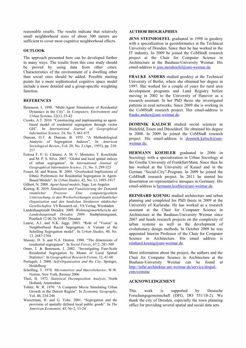
The best reproduction is achieved at a distance exponent

E of about 2.7. This value takes into account the

calculated segregation index values based on road

segments and on building blocks as shown in figure 5.

The road-segment-based Information Theory Index

HRoadSegment is displayed as the upper curve with a

dashed line. The lower curve shows the appropriate

building-block-based Index HBlock. The grey horizontal

lines display the target values for each index. Both

indices show a nearly strict dependency on E. The target

values are reached around E = 2.7, for HBlock between

2.6 and 2.7 and for HRoadSegment between 2.7 and 2.8.

If we use 2.7 as input for the dborder(E)-function (figure

4), a border distance of about just 27 meters results. In

our model a circle of this distance divides the close

neighbors that have 50% influence on the neighborhood

rating from those neighbors living further away that

make up the other 50% influence. Using the same

approach one can find a 90%-influence distance of

about 270 meters and a 99%-influence distance of about

7200 meters. Because relatively small changes of E can

lead to significant changes of the aforementioned

distance values, one could speak of 30, 300 and 7000

meters, respectively, as approximations.

Figure 5: Segregation Index H (the Information Theory

Index) Outcomes for Variation of Distance Exponent E

A major input of the simulation is the neighbor rating

function as described earlier in chapter TRANSITION

RULES, especially figure 3. To assess the influence,

tests have been run with an alternative neighbor rating

function. The social status rating function was set to be

identical to the one used for cultural rating, so that the

milieus strongly like living with neighbors from their

own milieu (rating value 1). Simulation experiments

with this setting result in a distance exponent E of about

1.8 for the best reproduction. This result contradicts our

theoretical expectations, because for E = 1.8 far

neighbors have in sum more influence than close ones.

CONCLUSION

Using the agent based simulation model developed here,

important segregation characteristics of a given data set

for the city of Dresden were successfully reproduced. It

has been shown that the milieu approach of social

grouping, a small set of neighbor rating rules and a

simple distance-dependent weighting function lead to

0,3500

0,4000

0,4500

0,5000

0,5500

0,6000

0,6500

0,7000

2 2,5 3 3,5 4

Se

gre

ga

tio

n I

nd

ex

H

Distance Exponent E

HRoadSegment

HBlock

target values

target value

reasonable results. The results indicate that relatively

small neighborhood sizes of about 300 meters are

sufficient to cover most cognitive neighborhood effects.

OUTLOOK

The approach presented here can be developed further

in many ways. The results from this case study should

be proved by using data from other cities.

Characteristics of the environment of a dwelling other

than social ones should be added. Possible starting

points for a more sophisticated cognitive space model

include a more detailed and a group-specific weighting

function.

REFERENCES

Benenson, I. 1998. “Multi-Agent Simulations of Residential

Dynamics in the City”. In Computers, Environment and

Urban Systems, 22(1), 25-42

Crooks, A.T. 2010. “Constructing and implementing an agent-

based model of residential segregation through vector

GIS”. In International Journal of Geographical

Information Science, 24, No. 5, 661-675

Duncan, O.T. & Duncan, B. 1955. “A Methodological

Analysis of Segregation Indexes”, In American

Sociological Review, Vol. 20, No. 2 (Apr., 1955), pp. 210-

217

Feitosa F. F; G. Câmara; A. M. V. Monteiro; T. Koschitzki

and M. P. S. Silva. 2007. “Global and local spatial indices

of urban segregation”. In International Journal of

Geographical Information Science, 21, No. 3, 299-323

Fosset, M. and Waren, W. 2005. “Overlooked Implications of

Ethnic Preferences for Residential Segregation in Agent-

Based Models”. In Urban Studies, 42, No. 11, 1893-1917

Gilbert, N. 2008. Agent-based models, Sage, Los Angeles

Koenig, R. 2010. Simulation und Visualisierung der Dynamik

räumlicher Prozesse: Eine computergestützte

Untersuchung zu den Wechselwirkungen sozialräumlicher

Organisation und den baulichen Strukturen städtischer

Gesellschaften. VS Research ed., VS Verlag, Wiesbaden

Landeshauptstadt Dresden. 2009. Wohnungsmarktbericht der

Landeshauptstadt Dresden 2009. Stadtplanungsamt,

Postfach 12 00 20, 01001 Dresden

Laurie, A.J. and N.K. Jaggi. 2003. “Role of “Vision” in

Neighborhood Racial Segregation: A Variant of the

Schelling Segregation model”. In Urban Studies, 40, No.

13, 2687-2704

Massay, D. S. and N.A. Denton. 1988. “The dimensions of

residential segregation”. In Social Forces, 67:2, 281-309

Omer, I. & Benenson, I. 2002. “Investigating Fine-Scale

Residential Segregation by Means of Local Spatial

Statistics”. In Geographical Research Forum, 12, 41-60

Portugali, J. 2000. Self-Organization and the City, Springer,

Heidelberg

Schelling, T. 1978. Micromotives and Macrobehavior, W.W.

Norton, New York, Reissue 2006

Theil, H. 1972. Statistical Decomposition Analysis, North

Holland, Amsterdam

Tobler, W. R. 1970. “A Computer Movie Simulating Urban

Growth in the Detroit Region”. In Economic Geography,

Vol. 46, 234-240

Wasserman, H. and G. Yohe. 2001. “Segregation and the

provision of spatially defined local public goods”. In The

American Economist, 45, No 2, 13-24

AUTHOR BIOGRAPHIES

JENS STEINHOEFEL graduated in 1998 in geodesy

with a specialization in geoinformatics at the Technical

University of Dresden. Since then he has worked in the

IT industry. In 2009 he joined the CoMStaR research

project at the Chair for Computer Science in

Architecture at the Bauhaus-University Weimar. His

email-address is jens.steinhoefel@uni-weimar.de.

FRAUKE ANDERS studied geodesy at the Technical

University of Berlin, where she obtained her degree in

1997. She worked for a couple of years for rural area

development programs and Land Registry before

moving in 2002 to the University of Hanover as a

research assistant. In her PhD thesis she investigated

patterns in road networks. Since 2009 she is working in

the CoMStaR research project. Her email-address is

frauke.anders@uni-weimar.de.

DOMINIK KALISCH studied social sciences in

Bielefeld, Essen and Düsseldorf. He obtained his degree

in 2008. In 2009 he joined the CoMStaR research

project. His email-address is dominik.kalisch@uni-

weimar.de.

HERMANN KOEHLER graduated in 2006 in

Sociology with a specialization in Urban Sociology at

the Goethe University of Frankfurt/Main. Since then he

has worked at the University of Kassel and in the

German “Social-City”-Program. In 2009 he joined the

CoMStaR research project. In 2011 he started his

dissertation on representative mosques in Germany. His

email-address is hermann.koehler@uni-weimar.de.

REINHARD KOENIG studied architecture and urban

planning and completed his PhD thesis in 2009 at the

University of Karlsruhe. He has worked as a research

assistant at the Chair for Computer Science in

Architecture at the Bauhaus-University Weimar since

2007 and heads research projects on the complexity of

urban systems as well as the development of

evolutionary design methods. In October 2009 he was

appointed Interim Professor of the Chair for Computer

Science in Architecture. His email address is

reinhard.koenig@uni-weimar.de.

More information about the project, the authors and the

Chair for Computer Science in Architecture at the

Bauhaus-University Weimar can be found at

http://infar.architektur.uni-weimar.de/service/drupal-

cms/comstar

ACKNOWLEDGEMENT

This work is supported by Deutsche

Forschungsgemeinschaft (DFG, DO 551/18-2). We

thank the city of Dresden, especially the town planning

office for providing several spatial and social data sets.