Investigation of Free SurfaceDamping Models withApplications to GapResonance ProblemsKevin MarkengMaster’s Thesis, Autumn 2015

Abstract

Resonant behaviour in the gap between two adjacent bodies on a free surfaceis investigated numerically. The study is done within the framework of two-dimensional potential theory. It is of common conception that traditional po-tential theory overpredicts the gap elevation around resonance due to neglectof viscous effects. In this study we consider empirical formulas for skin fric-tion, eddy damping and bilge keel damping, and include the effects by a freesurface damping model. A non-physical free surface damping model is also con-sidered, and the damping effects from the two models are compared. Some briefcomments are given on three-dimensional effects.

Contents

1 Introduction 21.1 Previous related studies . . . . . . . . . . . . . . . . . . . . . . . 21.2 Present study . . . . . . . . . . . . . . . . . . . . . . . . . . . . . 3

1.2.1 Scope . . . . . . . . . . . . . . . . . . . . . . . . . . . . . 3

2 Mathematical foundation 52.1 The boundary value problem . . . . . . . . . . . . . . . . . . . . 52.2 The Green function and Green’s theorem . . . . . . . . . . . . . 7

3 The Gap Resonance Problem 93.1 Relevance . . . . . . . . . . . . . . . . . . . . . . . . . . . . . . . 93.2 Resonant behaviour . . . . . . . . . . . . . . . . . . . . . . . . . 93.3 Zeroth order mode; the piston mode . . . . . . . . . . . . . . . . 103.4 Potential Damping . . . . . . . . . . . . . . . . . . . . . . . . . . 123.5 Viscous Damping Contributions . . . . . . . . . . . . . . . . . . . 12

3.5.1 Skin Friction damping . . . . . . . . . . . . . . . . . . . . 143.5.2 Eddy damping . . . . . . . . . . . . . . . . . . . . . . . . 143.5.3 Bilge keel damping . . . . . . . . . . . . . . . . . . . . . . 15

4 Free Surface Damping Models 164.1 Introduction . . . . . . . . . . . . . . . . . . . . . . . . . . . . . . 164.2 The Pressure Damping Model . . . . . . . . . . . . . . . . . . . . 16

4.2.1 Gap surface pressure distribution . . . . . . . . . . . . . . 174.2.2 Pressure generated potential . . . . . . . . . . . . . . . . 17

4.3 Newtonian Cooling . . . . . . . . . . . . . . . . . . . . . . . . . . 194.3.1 Applications . . . . . . . . . . . . . . . . . . . . . . . . . 194.3.2 Formulation . . . . . . . . . . . . . . . . . . . . . . . . . . 19

5 Numerical method and program structure 215.1 Boundary element method . . . . . . . . . . . . . . . . . . . . . . 21

5.1.1 System without additional damping . . . . . . . . . . . . 215.1.2 System with free surface damping . . . . . . . . . . . . . 23

5.2 Program structure . . . . . . . . . . . . . . . . . . . . . . . . . . 25

6 Numerical Analysis and Results 276.1 Introductory comment . . . . . . . . . . . . . . . . . . . . . . . . 276.2 The basis problem . . . . . . . . . . . . . . . . . . . . . . . . . . 27

6.2.1 Forced heave motion . . . . . . . . . . . . . . . . . . . . . 276.2.2 Incident wave upon rigid double-hull . . . . . . . . . . . . 31

1

6.2.3 Incident wave upon freely floating body . . . . . . . . . . 336.2.4 Comparison with 3D results from Wasim and comments

on three dimensional effects . . . . . . . . . . . . . . . . . 356.3 Free surface pressure model . . . . . . . . . . . . . . . . . . . . . 38

6.3.1 Introductory remarks . . . . . . . . . . . . . . . . . . . . 386.3.2 Heaving of rectangular boxes . . . . . . . . . . . . . . . . 39

6.4 Newtonian Cooling Damping Model . . . . . . . . . . . . . . . . 456.4.1 Heaving of rectangular boxes . . . . . . . . . . . . . . . . 45

6.5 Comparison of the damping models . . . . . . . . . . . . . . . . . 49

7 Summary and conclusion 51

Appendices 52

A Greens theorem 53

B Equivalent linearization 54

C Convergence test 55

D Equation of motion 56

2

ForordJeg ønsker å takke mine veiledere, professor John Grue og Dr. Scient TorgeirVada for oppfølging og veiledning i forbindelse med oppgaven. John Grue in-troduserte meg til fagfeltet hydrodynamikk, og hans engasjement og kunnskaphar vært en inspirasjonskilde gjennom hele studiet. Samarbeidet med TorgeirVada (Product Manager ved DNV GL Software) har ikke bare vært lærerikt,men også svært oppmuntrende.Min familie og kjæreste har vist stor interesse og støttet meg gjennom helestudiet, og for dette er jeg høyst takknemlig.Jeg vil takke alle på kontoret hos DNV GL for å ha latt meg gjeste kontoret, ogfor å ha gitt meg et innblikk i deres virksomhet. Spesielt takk til Peter, Kaijaog Styrk som har vært behjelpelige gjennom hele prosessen.En takk til Trond Svandal for mange gode diskusjoner rundt oppgavens tema.Til mine studiekamerater på lesesalen i 9. etasje ønsker jeg å takke for godtsamhold og god stemning, på tross av at quiz-laget vårt aldri ble en stor suksess.

1

Chapter 1

Introduction

When two or more structures are located in vicinity of each other, large resonantmotion may occure in the narrow gap between them. This may also be the caseif a single body has some sort of opening, for instance a moonpool. Gap surfaceresponse and hydrodynamic coefficients has proven to be a challenging task tocalculate accuratly for this particular problem.Seakeeping softwares based on the Boundary Element Method (BEM) is still themost popular engineering tool for analysing wave loads on marine structures.This is mainly due to high computer efficiency and the simplicity of defininggrid points. However, traditional BEM solvers does not take viscous effectsinto account. In certain applications, like resonant behaviour in narrow gaps ormoonpools, it has been demonstrated that viscous damping is important andshould not be neglected. The general conception is that the results acquiredfrom BEM solvers overpredict the fluid motion in the gap due to the neglectionof viscosity. The overpredicted fluid motion is also reflected in the pressureforces and may result in misleading conceptions of the situation.Viscous effects are best captured by Computational Fluid Dynamics (CFD) pro-grams which solves the Navier Stokes-equation. The grid required for analysingwave-body interaction within such a framework leads to computer heavy anal-ysis and high CPU time. Methods for including the effects of viscosity in themore effective BEM environment is therefore sought after.

1.1 Previous related studiesMany studies are devoted to gap resonance problems as it is relevant withinmarine activity. Molin [9] has provided an analytical expression for the loca-tion of the gap resonance frequency between rectangular boxes. However, toget amplitudes and transfer functions, the full problem must be solved numer-ically. Sun [14] analysized both the first order and the second order problemwith three dimensionsional potential theory. The non-linear effects were small,except for in some special cases in context with higher order resonance frequen-cies. Kristiansen and Faltinsen [7] solved the non-linear potential problem intwo dimensions, and applied an inviscid vortex tracking method in the BEM-formulation. The results were compared to model tests. They reported smallsecond order effects, and that the measured gap amplitude from the model test

2

were 1/3 of the calculated amplitude. They concluded that flow separation atthe bilges were the main reason for the discrepancy, and managed to get betteragreement with the use of the vortex tracking method. To provide externaldamping, a so called damping lid may be placed at the free surface in the gapor moonpool. Buchner et al. [2] used a rigid lid with a tunable damping ef-fect, while a flexible lid was provided by Newman [11]. A free surface dampingmethod was provided by Chen [3]. He introduced what is referred to as "poten-tial flow of fairly perfect fluid" into the BEM formulation. In his formulationthe provided damping is proportional to the velocity, but of opposite sign. Thedamping term is also proportional to a damping coefficient. The damping effectmust be tuned to the results match those from model tests.Recently, Kristiansen and Faltinsen [8] used a domain-decomposition method tostudy forced heave of a twin hull. The Navier-Stokes formulation was appliedin a domain close to the body while the rest of the fluid were treated by linearpotential theory. Their computed surface elevation amplitude matched verywell with experimental data. The method was reported as promising as itcaptures the important viscous effects without use of empirical input, and itis significantly faster than a full Navier-Stokes solver.

1.2 Present studyWe will investigate methods to correct the linearly overpredicted fluid motionat resconance frequencies in narrow gap problems. In particular we are focusingon the wave response occuring at the first resonance frequency, later referredto as the piston mode response. The study is done within the frames of BEM,as this is the current industry standard for wave-body analysis. We restrictourselves to a two-dimensional approach for practical purposes. We choose tofocus our attention on rigidly connected rectangular barges separated by a gap,as displayed in figure 1.1. In the BEM-formulation it is convinient to introducedamping in the free surface boundary condition. It is essential that the applieddamping is related to the actual physical viscous damping. Attention will begiven to energy dissipation. We use empirical formulas with strong foundationto estimate viscous forces. Two different free surface damping methods willbe investigated and compared. They are referred to as the Pressure DampingModel, and the Newtonian Cooling Damping Model.

1.2.1 Scope• Identify important aspects to gap resonance problems

• Give a general formulation of the Pressure Damping Model

• Find models for the damping due to viscous effects, and relate them tothe Pressure Damping Model

• Implement and investigate the Newtonian Cooling Damping Model, cur-rently used in HydroD Wasim

• Compare the two damping models

3

• Compare two-dimensional and three-dimensional computations. HydroDWasim will be used for three-dimensional computations

b

D

B BFigure 1.1: Two closely separated hulls. Each hull has a width B and draftD, and are separated by b. In this study the hulls are considered to be rigidlyconnected. This could be interpreted as the cross section of a barge with aninfinitely long moonpool. Throughout the thesis we will refere to the openingas the gap.

4

Chapter 2

Mathematical foundation

2.1 The boundary value problemWe consider a plane progressive wave of small amplitude interacting with afloating rigid body. The body will then undergo simple harmonic oscillationsdescribed by the body displacement from equilibrium . We assume irrotationaland incompressible flow, and apply linear potential theory. The velocity poten-tial Φ satisfies the Laplace equation in the fluid domain

∇2Φ = 0. (2.1)

All dynamic quantities are assumed to be harmonic in time, such that Φ maybe expressed as

Φ = Reϕeiωt, (2.2)

where Re denotes the real part and ω is the frequency of the incident wave.Similarly, all other quantities derived from ϕ is understood to be a complexamplitude and the physical values is the real part of the product between thecomplex amplitude and the time factor eiωt. We denote the free surface elevationas ζ, and define it as

ζ = Reηeiωt. (2.3)

Two conditions apply on the free surface, these are the kinematic and the dy-namic boundary conditions. The kinematic boundary condition requires thefluid velocity at the free surface to be the same as the surface velocity itself,

∂ζ

∂t=∂Φ

∂z. (2.4)

The linear dynamic condition follows from the linearized Bernoulli equation,

∂Φ

∂t+ gz = −1

ρp, (2.5)

by stating that the gauge pressure p is zero at the free surface and evaluatingat z = ζ,

5

∂Φ

∂t+ gζ = 0. (2.6)

The kinematic and dynamic boundary condition may be combined by differen-tiating (2.6) with respect to t and substitute (2.4), to form a single free surfaceboundary condition for Φ,

∂2Φ

∂t2+∂Φ

∂z= 0. (2.7)

By taking the time derivative and remove the time factor we may express theboundary condition in terms of the time independent potential ϕ,

−ω2

gϕ+

∂ϕ

∂z= 0. (2.8)

The fluid velocity at the body boundary follows the same velocity as the bound-ary itself,

∂Φ

∂n= U · n + Ω · (r× n), (2.9)

where n is the normal vector, r is the radius vector from center of rotation,U and Ω are the body translational velocity and the body angular velocityrespectively. If six degrees of freedom in three dimensions are considered, thecomponents of the body velocity are

Uj = Reiωξjeiωt j = 1, 2, ..., 6 (2.10)

where ξj is the complex amplitude, and j = 1, 2, ..., 6 is surge, sway, heave, roll,pitch and yaw respectively. In two dimensions the relevant degrees of freedomare j = 2, 3, 4.The velocity potential may be divided into a radiation potential and diffractionpotential, and summed by the super position principle

Φ = Re(ϕR + ϕD)eiωt. (2.11)

The radiation potential is due to the motion of the body while the diffractionpotential represents the incident wave and the disturbance due to the presenceof the body. The radiation potential is the sum of contributions from motionsin each degree of freedom. For motion in three dimensions we have

ϕR =

6∑j=1

ξjϕj , j = 1, 2, ..., 6 (2.12)

where ξj is the complex displacement amplitude. The body boundary conditionfor the radiation potentials follows from (2.9),

6

∂ϕj∂n

= iωnj j = 1, 2, 3

∂ϕj∂n

= iω(r× n)j−3 j = 4, 5, 6.

(2.13)

The diffraction potential consists of the incident wave potential ϕ0 with ampli-tude A, and the scattering wave potential ϕs which is due to the presence ofthe fixed body

ϕD = A(ϕ0 + ϕs), (2.14)

where ϕ0 is on the form

ϕ0 =ig

ωeky−ikx. (2.15)

As the body is considered fixed with respect to ϕD, the right hand side of (2.9)is zero. It follows that

∂ϕs∂n

= −∂ϕ0

∂n. (2.16)

As ϕj and ϕs is a consequence of the presence of the body, we must require thatthe associated waves radiates outwards from the body. This is the radiationcondition, and is necessary for uniqueness of the boundary value problem. Inthree dimensions we require

ϕj ∝ R−1/2e−ikR, as R →∞ j = 1, 2, ..., 6, s (2.17)

where R is the radial distance from the body. The two dimensional radiationcondition is

ϕj ∝ e∓ikx, as x → ±∞ j = 2, 3, 4, s. (2.18)

The boundary value problem defined by (2.1), (2.8), (2.13) and (2.16) will bereferred to as the basis problem.

2.2 The Green function and Green’s theoremDetails on the following is presented in Appendix A while a brief introductionis presented in this section. Green’s theorem may be utilized to form integralequations for unknown potentials. We introduce the Green function for infinitedepth in two dimensions [16],

G(x, ξ) = ln r1 − ln r2 − 2PV

∫ ∞0

1

k − ν ek(z+ζ) cos(k(x− ξ)) dk

+ 2πieν(z+ζ) cos(ν(x− ξ)),(2.19)

7

where r1 =√

(x− ξ)2 + (z − ζ)2, r2 =√

(x− ξ)2 + (z + ζ)2 and x = (x, z),ξ = (ξ, ζ) are understood to be coordinates in the two-dimensional plane. TheGreen function (2.19) represents a pulsating source potential at point ξ, evalu-ated at point x, and satisfies the free surface boundary condition (2.8) and theradiation condition (2.18). A fluid domain is illustrated in figure 2.1. ApplyingGreen’s theorem on the fluid domain to a unknown potential ϕ and G yields anintegral equation for ϕ,

∫S

(ϕ(ξ)

∂G(ξ; x)

∂nξ−G(ξ; x)

∂ϕ(ξ)

∂nξ

)dξ =

0, outside the fluid domainπϕ(x), on the boundary2πϕ(x), inside the fluid domain

(2.20)

The fact that (2.19) satisfy the free surface boundary conditions reduce theintegral to be taken only over the body surface. This is an essential feature ofthe Green function. Equation (A.4) may be used to form integral equations forthe unknown radiation and scattering potentials. Then ∂ϕ

∂n is known from theboundary conditions, and the equation is typically organized as

∫Sw

ϕ(ξ)∂G(ξ; x)

∂nξdξ −

(π

2π

)ϕ(x) =

∫Sw

G(ξ; x)∂ϕ(ξ)

∂nξdξ. (2.21)

Sw

Sf

Sx→−∞ Sx→∞

Sz→−∞

Fluid domain

Figure 2.1: Illustration of the fluid domain with boundary S = Sf+Sw+Sx→∞+Sx→−∞+Sz→−∞. The free surface is denoted by Sf , and Sw represents a rigidbody.

8

Chapter 3

The Gap Resonance Problem

3.1 RelevanceThe topic of this study applies to various marine applications. Gap resonancebehaviour may occure in situations where one or several structures bounds thefree surface in any manner. Some of the most important examples from themaritime industry beeing ships in side-by-side configuration, ship besides ter-minals relevant to on- and offloading operations, constructions with moonpoolsand multi-hull vessels.

3.2 Resonant behaviourWhen a structure encloses a part of the free surface, this enclosed free surfacewill be subject to violent motions at some frequencies of oscillation. We willrefere to the enclosed portion of the free surface as the gap surface. Motion ofthe gap surface may be trigged in three conceptual different scenarios. If thestructure is fixed, the gap surface motion can be trigged by an incident wave.Similarly, gap surface motion occurs if the body is forced to oscillate. We willfirst discuss these two cases, as they share some important similarities and givesimportent insight to the problem. Regardless if the gap surface oscillation iscaused by incident wave or forced body motion, there exists an infinite numberof what we will refere to as gap resonance frequencies. The gap surface will atthese frequencies undergo large motions, and the shape, or mode, of the surfacewill vary for each gap resonance frequency. The location of these frequenciesare only dependent on the geometrical shape of the body. The third case iswhen the body is free to respond to an incident wave field. Interestingly, thegap surface response at the gap resonant frequency is very small in this case.However, large elevation occurs when the structure itself undergo large motions.We will refere to the frequencies where peak structure response occurs as bodyresonance frequencies. It will later be clear that the structure response is indeeddependent on the gap resonance frequency.

9

3.3 Zeroth order mode; the piston modeAs discussed, each gap resonance frequency has its associated gap surface mode.There is one particular mode which in many ways differs from the others. Thisis the first mode occuring at the first gap resonance frequency, often referredto as the zeroth mode or the piston mode. At this mode, the gap surface isoscillating without variations across the gap. That is, the fluid in the gap ismoving with approximately uniform velocity and acts almost like a rigid body.As an counterexample, this resonant behaviour differs from that one mightexperience in a closed container. Linear resonant motion in a closed tank willconsist of purely antisymmetric sloshing modes due to mass conservation inthe tank. In the gap resonance problem the partially enclosed fluid is free tointeract, or communicate, with the rest of the fluid domain. See figure 3.1. Thiscommunication is an important aspect of the phenomenon.The piston mode will not necessarily be the first resonant mode encountered.For example, if a rigid body with a gap is forced to oscillate in sway, one shouldexpect that the first encountered resonant behaviour is at the second or thirdresonance frequency. The first resonance occuring in forced heave will alwaysbe the piston mode resonance. Examples of sway and heave induced motion areshown in figure 3.2 and 3.3.

Ωp

Communication

Figure 3.1: The "Piston body", or the partially enclosed fluid, is indicated bythe shaded area and denoted by Ωp. The important communication between thepartially enclosed fluid and the fluid outside the gap is indicated by the arrows.

10

−0.08 −0.06 −0.04 −0.02 0 0.02 0.04 0.06 0.08−0.5

0

0.5

1

1.5

Gap length

Piston mode behaviour

Figure 3.2: Example of heave induced piston modebehaviour. The surface elevation is displayed fora quarter of a periode, with grey lines indicatingprevious time steps.

−0.08 −0.06 −0.04 −0.02 0 0.02 0.04 0.06 0.08−0.5

−0.4

−0.3

−0.2

−0.1

0

0.1

0.2

0.3

0.4

0.5

Gap length

Sloshing mode behaviour

Figure 3.3: Example of sway induced sloshing be-haviour. The surface elevation is displayed for aquarter of a periode, with grey lines indicating pre-vious time steps.

11

3.4 Potential DampingPotential damping is associated with outgoing waves. When the resonant pistonmode elevation in the gap is trigged at the gap resonance frequency, the ampli-tude of oscillation will stay finite. This is a consequence of the communictionbetween the fluid in the gap and the external fluid. Energy will be trasportedaway from the structure with the outgoing waves. The generation of waves iscaptured by potential theory, and it is the sole source of damping if externaldamping mechanisms are not introduced.

3.5 Viscous Damping ContributionsIn many applications in marine hydrodynamics, viscous effects are consideredto be small, and therefore potential theory based codes proves to be a powerfultool. However, experiments suggests that this is not the case for the narrow gapproblem [7]. When potential calculations are compared to experimental data itshows clear tendencies that the potential calculations overpredict fluid veloci-ties. Many numerical studies have investigated the effect of non-linear potentialdamping with the conclusion that these effects are negligible for the piston modemotion [7][14]. It is of common conception that the discrepancy between po-tential solutions and experimental data is due to the lack of viscous dampingin the potential calculations. Viscous damping is considered to be of non-linearcharacter. As gap surface motion may become very large it is reasonable toexpect viscous damping to be a considerable contribution to the total damping.The viscous forces in play will in general dissipate energy, and hence both gapsurface elevation and body motions should be reduced. Accurate numerical cal-culations of the viscous effects can be demanding, and from a practical pointof view not feasible for large marine structures. Therefore, empirical formulaswhich approximates viscous effects is of great value.In context within marine hydrodynamics where viscous effects are of importance,one often seek to estimate the viscous drag force on moving bodies. In thepresent study, the main interest is the viscous damping of the piston-modeelevation. However, if a viscous drag force is acting on the body, a equal butopposite force is inflicted on the fluid.A quite general expression for the viscous force acting on a body ocillating inunbounded fluid is given by

FD =1

2ρL2CD|v|v, (3.1)

where ρ is the density of the fluid, v the relative velocity between the bodyand the fluid, L is a characteristic length and CD is a problem specific dragcoefficient. The drag coefficient will typically be a function of the Reynoldsnumber defined as

Re =vL

ν, (3.2)

where ν is the kinematic viscosity. The drag coefficient have to be empiricallydetermined. A number of experimental studies are devoted to this purpose, andreliable values for the drag coefficient is available for various applications.

12

As noted, (3.1) is based on the assumption that the fluid is unbounded. In ourproblem, a free surface is present. Nevertheless, we assume that the presence ofthe free surface has small effects on the viscous forces. Such an assumption isnot unusual. Equation (3.1) is often used to estimate viscous forces on jacketsand risers, and roll damping of ships or other structures where a free surface isindeed present.We will consider three different contributions to the viscous force acting on thepiston behaved fluid motion in the gap. These are the effect of skin friction,vortex shedding at the bilge, also reffered to as eddy making damping, andadditonal effect if bilge keels are present. Figure 3.4, 3.5 and 3.6 illustrates thedifferent effects. We may then express our total viscous force as

Fviscous = Fs + Fe + Fbk, (3.3)

where Fs, Fe, Fbk is the viscous force contribution due to skin friction, eddymaking and bilge keels, respectively. The three components will be furtherdiscussed in the following.

Ff

v

Figure 3.4: Illustration of frictionforce in the gap.

v

Fe

Figure 3.5: Illustration of vortexshedding at the bilge corners.

v

Fe + Fbk

Figure 3.6: Illustration of structurewith bilge keels. The presence ofbilge keels will typically intensifythe vortex shedding.

13

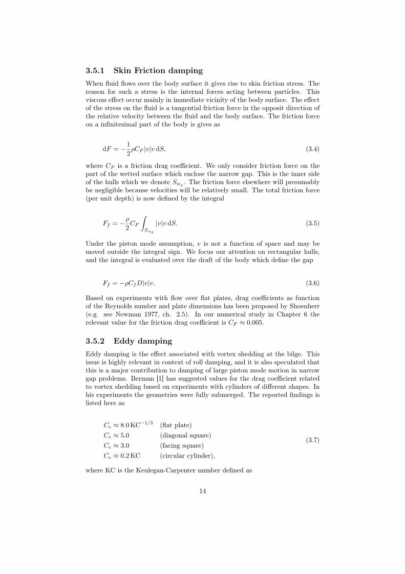
3.5.1 Skin Friction dampingWhen fluid flows over the body surface it gives rise to skin friction stress. Thereason for such a stress is the internal forces acting between particles. Thisviscous effect occur mainly in immediate vicinity of the body surface. The effectof the stress on the fluid is a tangential friction force in the opposit direction ofthe relative velocity between the fluid and the body surface. The friction forceon a infinitesimal part of the body is gives as

dF = −1

2ρCF |v|v dS, (3.4)

where CF is a friction drag coefficient. We only consider friction force on thepart of the wetted surface which enclose the narrow gap. This is the inner sideof the hulls which we denote Swg

. The friction force elsewhere will presumablybe negligible because velocities will be relatively small. The total friction force(per unit depth) is now defined by the integral

Ff = −ρ2CF

∫Swg

|v|v dS. (3.5)

Under the piston mode assumption, v is not a function of space and may bemoved outside the integral sign. We focus our attention on rectangular hulls,and the integral is evaluated over the draft of the body which define the gap

Ff = −ρCfD|v|v. (3.6)

Based on experiments with flow over flat plates, drag coefficients as functionof the Reynolds number and plate dimensions has been proposed by Shoenherr(e.g. see Newman 1977, ch. 2.5). In our numerical study in Chapter 6 therelevant value for the friction drag coefficient is CF ≈ 0.005.

3.5.2 Eddy dampingEddy damping is the effect associated with vortex shedding at the bilge. Thisissue is highly relevant in context of roll damping, and it is also speculated thatthis is a major contribution to damping of large piston mode motion in narrowgap problems. Berman [1] has suggested values for the drag coefficient relatedto vortex shedding based on experiments with cylinders of different shapes. Inhis experiments the geometries were fully submerged. The reported findings islisted here as

Ce ≈ 8.0 KC−1/3 (flat plate)Ce ≈ 5.0 (diagonal square)Ce ≈ 3.0 (facing square)Ce ≈ 0.2 KC (circular cylinder),

(3.7)

where KC is the Keulegan-Carpenter number defined as

14

KC =VmaxT

Lc(3.8)

where T is the period of oscillation and Umax is the maximum velocity.To the present study, the coefficient for diagonal square is relevant. To makeuse of the values for Ce in (3.7), some assumptions have to be made. We assumethat the vortex shedding from the bilge corners is a local effect, such that thebilge corners may be regarded as fully submerged. We also assume that theeffect of the two corners facing the gap is equivalent to 1/2 of the effect of thefacing square in (3.7), with the width of the square as the characteristic length.This means that we regard the vortex shedding effect from each corner in (3.7)as equal. These may be regarded as quite rough estimates, but nevertheless wehope to capture the leading effect. The expression for the eddy making force(per unit depth) is then given by

Fe = −1

2ρB

Ce2|v|v (3.9)

with Ce = 3.0.

3.5.3 Bilge keel dampingShips are often equipped with bilge keels to reduce roll response. The bilge keelsintroduce viscous damping mainly due to vortex shedding. When these keelsare interacting with the large fluid motion in narrow gap, it should be expectedthat the viscous effects from the keels is an important damping contribution ofthe piston-like fluid motion. We consider two bilge keels as in figure 3.6, eachwith width Bbk. We apply the flat plate drag coefficient from (3.7), and do theassumption that the effect of the two keels, each with width Bbk and one endpointed out in the stream, equals the effect of a flat plate with width 2Bbk withtwo open ends. The viscous force from the bilge keels on the fluid (per unitdepth) is expressed as

Fbk = −1

2ρCe2Bbk|v|v, (3.10)

with Ce = 8.0 KC−1/3.

15

Chapter 4

Free Surface Damping Models

4.1 IntroductionThe energy will always be conserved in the traditional potential formulation.This is an unphysical characteristics of the potential formulation, but it is oftenrightfully justified by assuming that dissipative effects are small. However, en-ergy will dissipate if the fluid is viscous. It is stated that viscous effects shouldnot be neglected if a narrow gap is present [5][7]. The forces due to viscouseffects were discussed in chapter 3, and it was indicated that they will resultin decreased free surface elevation in the gap. In this chapter we formulatetwo methods which provide additional damping of the free surface elevation.They are referred to as the Pressure Damping Model and the Newtonian Cool-ing damping model. The methods are within the framework of potential theory,and external damping is introduced in the free surface boundary condition. ThePressure Damping Model will be directly related to the viscous forces consideredin chapter 3, while the other method is of empirical character. Both methodswill dissipate energy from the system.

4.2 The Pressure Damping ModelThe Pressure Surface method has been used to study the OWC (OscillatingWater Column) wave energy devices, and surface effect ships [13][15]. In thosecases, a pressure due to fans or compressed air will be distributed on an areaof the free surface. We will utilize this method and relate the pressure force tothe viscous forces analyzed in chapter 3. It is important to emphasize that nophysical pressure is acting on the gap surface in our problem. However, whenthe gap is narrow we assume that viscous forces acting in the gap will have anapproximatly uniform damping effect on the piston-like fluid response.

16

4.2.1 Gap surface pressure distributionIn Chapter 3 we considered viscous forces in the gap on the general formFviscous = − 1

2ρL2cCD|v|v. We assume that the effect on the piston mode motion

in the gap will be uniform and expresses the force as a pressure distribution onthe gap surface,

P = −Fviscousb

, (4.1)

where b is the gap length from figure 1.1. The pressure will now be on thegeneral form

P =1

2ρL2c

bCD|v|v (4.2)

The expression may be linearized by the method of equivalent linearization.Details on the procedure is given in Appendix B. (4.2) can then be expressedas

P ≈ 4

3πρCDV0

L2c

bv. (4.3)

It is important to note that expression (4.3) is still quadratic in amplitude. Aswe assume the fluid velocity v to be uniform in the gap, the velocity is relatedto the potential and the elevation through (2.4),

v =∂Φ

∂z=∂ζ

∂t. (4.4)

P may then be expressed as

P = Repeiωt = Re 4

3πρCD|iωη|

L2c

biωη eiωt. (4.5)

The velocity is taken to be the velocity from the basis problem, without anyadditional free surface damping.Note: By the numerical study on forced heave motion conducted in section 6.3,we have reached the conclusion that the pressure should have the phase of thebody motion rather than the fluid gap velocity to get the desired effect. See thediscussion in section 6.3.1.

4.2.2 Pressure generated potentialWhen pressure is acting on the free surface, the following boundary conditionapply

−ω2

gϕp +

∂ϕp∂z

= − iωρgp, (4.6)

17

where ϕp is the pressure generated potential. The pressure is introduced onthe gap surface. The total potential (2.11) is thereby extended to include thevelocity potentials due to free surface pressure in the gap

Φ = Re(ϕR + ϕD + ϕp)eiωt, (4.7)

where ϕp is the pressure generated potential. The introduction of the pres-sure generated potentials requires additional boundary conditions to the originalboundary value problem. On the wetted surface we have

ϕp∂n

= 0. (4.8)

On the gap surface the pressure generated potential fulfill (4.6) while (2.8) holdsfor the potentials generated from body motion and scattering.The field equation (2.1) and the free surface condition outside the body (2.8) isunchanged. Note that for the potentials generated from motion of the body, aswell as for the diffraction potential, the boundary value problem is unchanged.These potentials can be solved separately by (2.21) without any additions. Forthe pressure generated potential and its boundary conditions some modificationsto the integral equations are required. The Green function does not satisfy thegap surface condition for ϕp and thus the integral does not vanish as in (2.21).The integral is extended to include the gap surface Sg,

(π

2π

)ϕp(x) =

∫Sw+Sg

(ϕp(ξ)

∂G(ξ; x)

∂nξ−G(ξ; x)

∂ϕp(ξ)

∂nξ

)dξ . (4.9)

Here we substitute the boundary conditions (4.6) and (4.8)

(π

2π

)ϕp(x) =

∫Sw

ϕp(ξ)∂G(ξ; x)

∂nξdξ

+

∫Sg

(ϕp(ξ)

ω2

gG(ξ; x)−G(ξ; x)

(ω2

gϕp(x)− iω

ρgp

))dξ,

(4.10)

which reduce to(π

2π

)ϕp(x) =

∫Sw

ϕp(ξ)∂G(ξ; x)

∂nξdξ +

∫Sg

G(ξ,x)iω

ρgp dξ. (4.11)

We organize the equation to arrive at

∫Sw

ϕp(ξ)∂G(ξ; x)

∂nξdξ −

(π

2π

)ϕp(x) = −

∫Sg

G(ξ,x)iω

ρgp dξ. (4.12)

18

4.3 Newtonian Cooling

4.3.1 ApplicationsNumerical beach

Newtonian Cooling is primarily used in context with Numerical beaches [6].Numerical wave tanks are often used to analyse wave-body interaction in thetime domain. To avoid reflections from the boundaries of the tank, so callednumerical beaches are often applied. A numerical beach is a damping zone,where typically the wave motion is eventually damped to zero such that a ho-mogenous Neumann boundary condition may be applied on tank boundary. Inthe damping zone, a dissipative term is added to the kinematic free surfaceboundary condition. The dissipative term, or damping term, is proportional tosome damping coefficient. The damping coefficient is typically a smooth func-tion varying with x. It is zero at the inner boundary of the damping zone andsmoothly increases outwards until all motions are damped out.

Narrow gaps and moonpools

The Newtonian cooling method is also used as a source of external dampingof fluid motion in moonpools and narrow gaps. The damping coefficient isset constant and the modified kinematic boundary condition which include thedamping term is applied on the free surface in the gap, or moonpool. From apractical point of view, the method is relatively easy to implement in a potentialsolver. The additional damping introduced is, as we will see in our numericalstudy, well behaved and easy to control. However, the damping is of purelymathematical character and has no foundation in physics. The physical dampingmay vary greatly depending on the geometry and sea state, so the level ofdamping is often tuned to match those from model tests.

4.3.2 FormulationThe kinematic free surface condition is modified to include a damping term

∂ζ

∂t=∂Φ

∂z− 2νζ +

ν2

gΦ. (4.13)

The first additional term gives damping while the second ensures that the disper-sion relation is unchanged. The additional damping is of purely mathematicalcharacter and is not related to physics. The coefficient ν will decide the levelof damping and must be experimentally determined. Both the dynamic freesurface boundary condition and the kinematic body boundary condition is un-changed. Combination of the kinematic and dynamic boundary condition givesthe free surface condition

∂2Φ

∂t2+ g

(∂Φ

∂z+

2ν

g

∂Φ

∂t+ν2

gΦ

)= 0. (4.14)

Notice that the Green function does not satisfy this free surface condition, anda free surface integral is required,

19

(π

2π

)ϕ(x) =

∫Sw+Sg

(ϕ(ξ)

∂G(ξ; x)

∂nξ−G(ξ; x)

∂ϕ(ξ)

∂nξ

)dξ . (4.15)

We express the free surface boundary condition (4.14) in terms of the timeindependent potential

∂ϕ

∂z=ω2

gϕ− 2ν

iω

gϕ− ν2

gϕ, (4.16)

and substitute (4.16) in the integral equation (4.15),

∫Sw

ϕ(ξ)∂G(ξ; x)

∂nξdξ +

∫Sg

ϕ(ξ)G(ξ; x)

(2νiω

g+ν2

g

)dξ −

(π

2π

)ϕ(x)

=

∫Sw

G(ξ,x)∂ϕ(ξ)

∂nξdξ

(4.17)

We note that ϕ is an unknown on the wetted boundary and the gap surface atthe same time regardless of the location of x.

20

Chapter 5

Numerical method andprogram structure

5.1 Boundary element methodWe distinguish between two different methods frequently used within BEM tosolve potential theory problems. Those are the potential formulation and thesource formulation. The potential formulation is often the method of choicewhen the free surface Green function is known, and its derivatives and integralsare easily evaluated. As noted in 2.2, the proper choice of Green function tradi-tionally reduce the integrals to be taken only over the body surface, as the freesurface integral is zero. In the source formulation one use the simple Rankinesource and seek to determine its strength. However, this requires meshing ofthe free surface. In the present study we are applying the potential formulationto solve the Laplace equation together with the given boundary conditions. Thepotential formulation utilize the fact that Greens theorem may be used to for-mulate integral equations for the unknown velocity potential. We have alreadydeveloped the integral equations for our desired potential solutions in Chapter4, as well as for the basis problem in 2.2. These equations are discretisized toform a linear set of algebraic equations. Typically, the body surface is dividedinto N segments, or panels. A panel distribution is illustrated in figure 5.1.Over each of these panels the velocity potential is assumed constant. The pointwhere the potential is to be evaluated is referred to as the field point xi, whilesingularities are distributed at the source points ξj . The singularities are thepulsating source and dipole, given as the Green function (2.19) and its nor-mal derivative. The numerical integrals over each panel are often carried outwith Gaussian quadrature. This technique yields better convergence than forexample the trapezoidal rule. In general more panels are required for the lattermethod. However, in our implementation we are using the trapezoidal rule forsimplicity. Convergence is demonstrated in Appendix C.

5.1.1 System without additional dampingFirst, the general procedure are presented for the traditional integral equation(2.21) without additional free surface terms. We consider the field point xi on

21

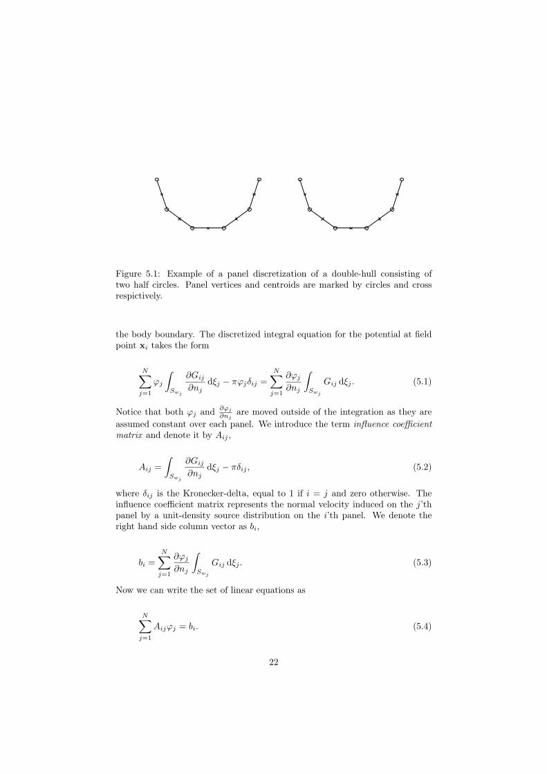
Figure 5.1: Example of a panel discretization of a double-hull consisting oftwo half circles. Panel vertices and centroids are marked by circles and crossrespictively.

the body boundary. The discretized integral equation for the potential at fieldpoint xi takes the form

N∑j=1

ϕj

∫Swj

∂Gij∂nj

dξj − πϕjδij =

N∑j=1

∂ϕj∂nj

∫Swj

Gij dξj . (5.1)

Notice that both ϕj and ∂ϕj

∂njare moved outside of the integration as they are

assumed constant over each panel. We introduce the term influence coefficientmatrix and denote it by Aij ,

Aij =

∫Swj

∂Gij∂nj

dξj − πδij , (5.2)

where δij is the Kronecker-delta, equal to 1 if i = j and zero otherwise. Theinfluence coefficient matrix represents the normal velocity induced on the j’thpanel by a unit-density source distribution on the i’th panel. We denote theright hand side column vector as bi,

bi =

N∑j=1

∂ϕj∂nj

∫Swj

Gij dξj . (5.3)

Now we can write the set of linear equations as

N∑j=1

Aijϕj = bi. (5.4)

22

This matrix equation is solved by Gaussian elemination.When the potential on the body is known, (5.1) can be used to find the potentialat field point xl located anywhere in the fluid.

ϕl =1

2π

N∑j=1

∫Swj

(ϕj∂Glj∂nj

−Glj∂ϕj∂nj

)dξj . (5.5)

The potential solution in the gap is necessary to compute the gap surface ele-vation. To get a continous representation of the solution we discretize the gapsurface Sg into M panels, and solve (5.5) for each l on Sg .

5.1.2 System with free surface dampingIn the integral equations for the free surface damping methods, a non-zero freesurface integral is present in the gap. This requires paneling of the gap surfaceand additional gap surface integrals are introduced. We denote field points onSg by l and the source points by k.

Integral equations for the Pressure Damping Model

The total pressure damped solution is expressed as a superposition of the radi-ation potential, the diffraction potential and the pressure generated potential.The radiation and diffraction potential is the same as in the system without ad-ditional damping and the solution procedure is discribed by 5.1.1. The integralequation for the pressure generated potential is given in (4.12). We discretize itin a similar manner as (5.1). For x on Sw we get

N∑j=1

ϕpj

∫SWj

∂Gij∂nj

dξj − πϕpjδij = −M∑k=1

iω

ρgp

∫Sgk

Gik dξk, (5.6)

while the equation for x on Sg is given by

N∑j=1

ϕpj

∫SWj

∂Glj∂nj

dξj − 2πϕpjδlk = −M∑k=1

iω

ρgp

∫Sgk

Glk dξk. (5.7)

The left hand side matrix in (5.6) is identical to that in (5.1), while the righthand side is the contribution from the non-zero gap surface integral. When pis a function of the velocity obtained from the basis problem, as in (4.5), it isrequired that(5.1) and (5.5) is solved at first.

Integral equations for the Newtonian cooling model

The additional Newtonian cooling terms affect the left hand side of the integralequation (5.8), as the new terms contains the unknown velocity potential. Forx on Sw the discretisized equation reads

23

N∑j=1

(ϕj

∫Swj

∂Gij∂nj

dξj − πϕjδij) +

M∑k=1

ϕk

∫Sgk

Gik

(2νiω

g+ν2

g

)dξk

=

N∑j=1

∂ϕj∂nj

∫Swj

Gij dξj

(5.8)

For x on Sg we get the following

N∑j=1

ϕj

∫Swj

∂Glj∂nj

dξj +

M∑k=1

(ϕk

∫Sgk

Glk

(2νiω

g+ν2

g

)dξk − 2πϕjδlk)

=

N∑j=1

∂ϕj∂nj

∫Swj

Glj dξj

(5.9)

The two equations, 5.8 and 5.9, must be solved simultaneously due to that thevelocity potential is unknown on both Sw and Sg regardless of the location ofx. The matrix equation Aϕ = b is arranged as

(A BC D

)(ϕ1

ϕ2

)=

(b1b2

)(5.10)

where elements of A and b1 is given in 5.2 and 5.3, while the rest of the vectorsand matrices are given as

Bik =

∫Sgk

Gik(2ν

giω +

ν2

g) dξk (5.11)

Clj =

∫Swj

∂Glj∂nj

dξj (5.12)

Dlk = −2πδlk +

∫Sgk

Glk(2ν

giω +

ν2

g) dξk (5.13)

b2,l =

N∑j=1

∂ϕj∂nj

∫Swj

Glj dξj , (5.14)

ϕ1,j = ϕj , (5.15)

ϕ2,k = ϕk, (5.16)

for i, j = 1, ..., N and l, k = 1, ...,M .

24

5.2 Program structureIt is appropriate to demonstrate how both the additional damping methods maybe included in a traditional BEM potential solver. Our approach is based onthat equation (5.1) and (5.5) are solved at first by our basis solver. As notedin 5.1.2, the influence coefficient matrices and right hand side vectors in thePressure Damping model and the Newtonian cooling model, are equal or par-tially equal those in the basis problem. This enables opportunities for effectivefree surface damping solvers as add-ons to the basis solver. The layout for theBEM-code developed for the present study is outlined in figure 5.2.

Note: Parts of the basis solver were developed by the author in an earlierproject work, while the rest of the program were developed during the workwith this thesis.

25

Basis solver

Pressure surface

Newtonian cooling

Boundary potentials

Field potentials

Boundary potentials

Field potentials

Boundary potentials

Input parameters

Geometry

Post-processing

Force calculations

Equation of motion

Wave elevation

Energy calculations

ϕP

ϕ

ϕνAij, bi

Aij, ϕ

and field potentials

(coupled solution)

Figure 5.2: Program structure of the BEM code developed for this thesis.

26

Chapter 6

Numerical Analysis andResults

6.1 Introductory commentThe author is aware of that the computed gap wave elevation in the basisproblem is not completely consistent with those presented by Kristiansen andFaltinsen [8]. Their reported amplitude at resonance in forced heave motion isAg/|ξ3| ≈ 13, while our calculations produce an amplitude Ag/|ξ3| ≈ 16. De-spite this, the gap resonance frequency and the far-field amplitude shows goodcorrespondence. The cause of the disagreement for the gap resonance ampli-tude has not been found. Different results from our code is controlled by energyconsiderations and far-field relations in the following sections, and convergenceis demonstrated in Appendix C.

6.2 The basis problemWe will first present results from our analysis of wave-body interaction whenno additional damping is applied in the gap. Although the calculations withoutany additional damping overpredict the gap elevation, it will provide importantunderstanding of the dynamics and the interaction between different parts ofthe system. We do a complete analysis of a double-hull, including the radiationand diffraction subproblems, and the situation when the body is freely floating.We seek to illustrate the previously described gap resonance, body resonanceand their interaction. Energy and farfield relations will serve as code validation.Some of our results will also be compared to output from the three-dimensionalpotential solver Wasim provided by DNV GL Software. In this context three-dimensional effects will be briefly discussed.

6.2.1 Forced heave motionIn the radiation problem we solve the velocity potentials due to forced bodymotion in the relevant degrees of freedom. In the two-dimensional case we havethree degrees of freedom, namely heave, sway and roll. Only heave motion willcontribute to the piston mode elevation, as sway and roll motion will result in

27

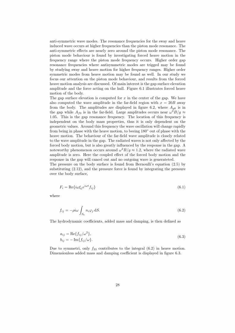
anti-symmetric wave modes. The resonance frequencies for the sway and heaveinduced wave occurs at higher frequencies than the piston mode resonance. Theanti-symmetric effects are nearly zero around the piston mode resonance. Thepiston mode behaviour is found by investigating forced heave motion in thefrequency range where the piston mode frequency occurs. Higher order gapresonance frequencies where antisymmetric modes are trigged may be foundby studying sway and heave motion for higher frequency ranges. Higher ordersymmetric modes from heave motion may be found as well. In our study wefocus our attention on the piston mode behaviour, and results from the forcedheave motion analysis are discussed. Of main interest is the gap surface elevationamplitude and the force acting on the hull. Figure 6.1 illustrates forced heavemotion of the body.The gap surface elevation is computed for x in the center of the gap. We havealso computed the wave amplitude in the far-field region with x = 20B awayfrom the body. The amplitudes are displayed in figure 6.2, where Ag0 is inthe gap while Af0 is in the far-field. Large amplitudes occurs near ω2B/g ≈1.05. This is the gap resonance frequency. The location of this frequency isindependent on the body mass properties, thus it is only dependent on thegeometric values. Around this frequency the wave oscillation will change rapidlyfrom being in phase with the heave motion, to beeing 180 out of phase with theheave motion. The behaviour of the far-field wave amplitude is closely relatedto the wave amplitude in the gap. The radiated waves is not only affected by theforced body motion, but is also greatly influenced by the response in the gap. Anoteworthy phenomenon occurs around ω2B/g ≈ 1.2, where the radiated waveamplitude is zero. Here the coupled effect of the forced body motion and theresponse in the gap will cancel out and no outgoing wave is generateted.The pressure on the body surface is found from Bernoulli’s equation (2.5) bysubstituting (2.12), and the pressure force is found by integrating the pressureover the body surface,

Fi = Reiωξjeiωtfij (6.1)

where

fij = −ρiω∫Sb

niϕj dS. (6.2)

The hydrodynamic coefficients, added mass and damping, is then defined as

aij = Refij/ω2,bij = − Imfij/ω.

(6.3)

Due to symmetri, only f33 contributes to the integral (6.2) in heave motion.Dimensionless added mass and damping coefficient is displayed in figure 6.3.

28

ξ3 ξ3

η3

dEdt

dEdt

Figure 6.1: Forced heave motion with forcing amplitude |ξ3|. The forced body motiongenerates oscillation in the gap, and radiated waves with mean energy flux dE

dt . Our maininterest is the wave amplitude |η3| in the gap.

0.6 0.7 0.8 0.9 1 1.1 1.2 1.3 1.4 1.5 1.60

2

4

6

8

10

12

14

16

ω 2

gB

Ag0

/|ξ3|

Af0

/|ξ3|

Figure 6.2: Wave amplitude Ag0 = |η3| in the gap, andAf0 = |η3| in the far field, relative to the forcing ampli-tude |ξ3|. B/D = 2, b/D = 1.

0.6 0.7 0.8 0.9 1 1.1 1.2 1.3 1.4 1.5 1.6−4

−3

−2

−1

0

1

2

3

ω 2

gB

Scaled added mass coefficient

Scaled damping coefficient

Figure 6.3: Hydrodynamic coefficients. Scaled addedmass coefficient a33/ρB

2, and scaled damping coeffi-cient b33/(ρB

2√ρB).

29

The damping coefficient is directly related to the energy of the outgoing waves.The average work done by the body on the fluid over one period is given as

W = −F3U3 =1

2ω2b33|ξ|2. (6.4)

The energy added to the waves must radiate outwards and may alternativelybe found by computing the energy flux in the far field. For infinite depth, theaverage energy flux is

dE

dt= VgE, (6.5)

where Vg is the group velocity and the energy density E is given by

E =1

2ρgA2

f , (6.6)

where Af is the far-field amplitude. In this context, this relation will serve asan excellent code check. Computed values of (6.12) and (6.5) is shown in figure6.4.

0.6 0.7 0.8 0.9 1 1.1 1.2 1.3 1.4 1.5 1.60

1

2

3

4

5

6

7

8

9

10

ω 2

gB

Average far−field energy flux (scaled)

Average work done by the body (scaled)

Figure 6.4: Average work done over one period scaled as W/(ρBg√Bg), and

average energyflux over one period scaled as dEdt /(ρBg

√Bg).

30

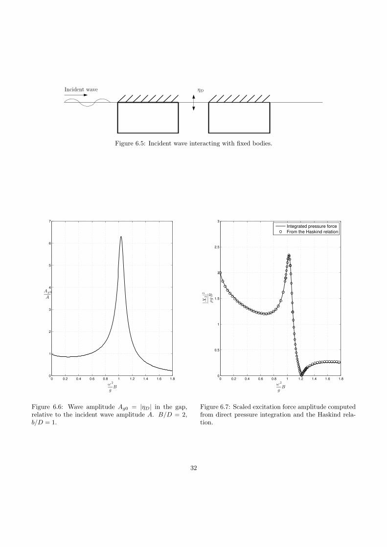
6.2.2 Incident wave upon rigid double-hullWe let an incident wave interact with the body when it is restrained frommoving. This is the diffraction problem, illustrated in figure 6.5. The incidentwave will induce wave motion in the gap. The computed amplitude is shown infigure 6.6. The peak amplitude occur at the gap resonance frequency.The pressure is found from Bernoulli’s equation (2.5) by substituting (2.14), andthe excitation force is found by integrating the pressure over the body surface,

Fi = ReAXieiωt (6.7)

where the complex amplitude Xi is defined as

Xi = −ρ∫Sw

(ϕ0 + ϕs) dS. (6.8)

An alternative formulation for the excitation force is given from the Haskindrelation (e.g. see Newman 1977, ch. 6.18) as

|Xi|2 = 2ρgVgbii. (6.9)

In amplitude of the exciting force is displayed in figure 6.7, where it has beencomputed using 6.8 and 6.9.

31

ηDIncident wave

Figure 6.5: Incident wave interacting with fixed bodies.

0 0.2 0.4 0.6 0.8 1 1.2 1.4 1.6 1.80

1

2

3

4

5

6

7

Ag 0

A

ω 2

gB

Figure 6.6: Wave amplitude Ag0 = |ηD| in the gap,relative to the incident wave amplitude A. B/D = 2,b/D = 1.

0 0.2 0.4 0.6 0.8 1 1.2 1.4 1.6 1.80

0.5

1

1.5

2

2.5

3

ω 2

gB

|X3|2

ρgB

Integrated pressure force

From the Haskind relation

Figure 6.7: Scaled excitation force amplitude computedfrom direct pressure integration and the Haskind rela-tion.

32

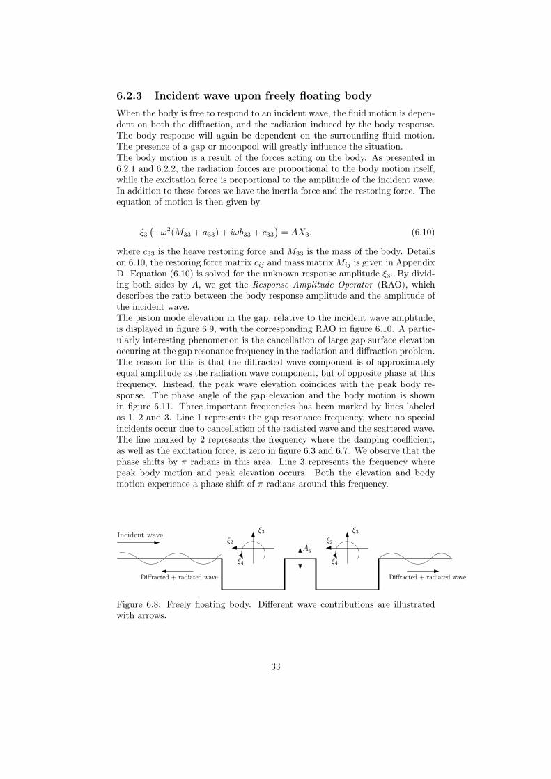
6.2.3 Incident wave upon freely floating bodyWhen the body is free to respond to an incident wave, the fluid motion is depen-dent on both the diffraction, and the radiation induced by the body response.The body response will again be dependent on the surrounding fluid motion.The presence of a gap or moonpool will greatly influence the situation.The body motion is a result of the forces acting on the body. As presented in6.2.1 and 6.2.2, the radiation forces are proportional to the body motion itself,while the excitation force is proportional to the amplitude of the incident wave.In addition to these forces we have the inertia force and the restoring force. Theequation of motion is then given by

ξ3(−ω2(M33 + a33) + iωb33 + c33

)= AX3, (6.10)

where c33 is the heave restoring force and M33 is the mass of the body. Detailson 6.10, the restoring force matrix cij and mass matrixMij is given in AppendixD. Equation (6.10) is solved for the unknown response amplitude ξ3. By divid-ing both sides by A, we get the Response Amplitude Operator (RAO), whichdescribes the ratio between the body response amplitude and the amplitude ofthe incident wave.The piston mode elevation in the gap, relative to the incident wave amplitude,is displayed in figure 6.9, with the corresponding RAO in figure 6.10. A partic-ularly interesting phenomenon is the cancellation of large gap surface elevationoccuring at the gap resonance frequency in the radiation and diffraction problem.The reason for this is that the diffracted wave component is of approximatelyequal amplitude as the radiation wave component, but of opposite phase at thisfrequency. Instead, the peak wave elevation coincides with the peak body re-sponse. The phase angle of the gap elevation and the body motion is shownin figure 6.11. Three important frequencies has been marked by lines labeledas 1, 2 and 3. Line 1 represents the gap resonance frequency, where no specialincidents occur due to cancellation of the radiated wave and the scattered wave.The line marked by 2 represents the frequency where the damping coefficient,as well as the excitation force, is zero in figure 6.3 and 6.7. We observe that thephase shifts by π radians in this area. Line 3 represents the frequency wherepeak body motion and peak elevation occurs. Both the elevation and bodymotion experience a phase shift of π radians around this frequency.

Incident waveξ3

ξ2

ξ4

ξ3ξ2

ξ4

Ag

Diffracted + radiated wave Diffracted + radiated wave

Figure 6.8: Freely floating body. Different wave contributions are illustratedwith arrows.

33

0 0.2 0.4 0.6 0.8 1 1.2 1.4 1.6 1.80

1

2

3

4

5

6

7

Ag

A

ω 2

gB

Figure 6.9: Wave elevation in gap. B/D = 2, b/D = 1.

0 0.2 0.4 0.6 0.8 1 1.2 1.4 1.6 1.80

0.5

1

1.5

2

2.5

3

|ξ3|

A

ω 2

gB

1 2 3

Figure 6.10: Heave response amplitude operator. Thelines marked by 1, 2 and 3 indicates the gap resonancefrequency, the frequency where the damping is zero,and the peak body responce frequency respectively.B/D = 2, b/D = 1.

0.6 0.8 1 1.2 1.4 1.6 1.8−5

−4

−3

−2

−1

0

1

2

3

θ

ω 2

gB

31 2

Phase of gap wave

Phase of body motion

Figure 6.11: Phase of the body motion and the piston-like elevation in the gap. The lines marked by 1, 2 and3 indicates the gap resonance frequency, the frequencywhere the damping is zero, and the peak body responcefrequency respectively. B/D = 2, b/D = 1.

34

6.2.4 Comparison with 3D results from Wasim and com-ments on three dimensional effects

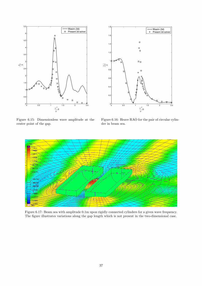
By comparing results from the two dimensional (2D) case to those from a threedimensional (3D) analysis, insigths to three dimensional effects is obtained. The3D computations are performed with the time domain potential solver Wasimfrom the HydroD package provided by DNV GL Software. The investigated caseis similar to the 2D analysis presented in 6.2.3, but with circular cylinders. A2D analysis with equivalent cross section were done to get comparable results.The three dimensional floating body consists of two rigidly connected half cir-cular cylinders with length L = 10 m, radius R = 1 m and with a gap widthb = 0.8 m. The geometry and the panel mesh is displayed in figure 6.12, 6.13and 6.14.The body is free to respond to beam sea in heave while the other degrees offreedom are restrained. Obtained heave response is still the same as the oneobtained if the body were freely floating. More specifically, pitch and surge iszero due to symmertry, while there is no coupling between heave and sway, orheave and roll.The wave amplitude at the center of the gap is displayed together with theresult from 2D computations in figure 6.17. The heave response is shown infigure 6.16. Both the 3D computed wave amplitude and heave RAO shows goodresemblance to the ones from the 2D case, but with some evident differences.Differences is to be expected as the three dimensional case allows for variationof the elevation in the gap length direction. In the region ω2R/g ≈ 1.5 toω2R/g = 2.5 the wave amplitude in 3D shows local maximums with fairly largeamplitude whereas the 2D amplitude is relatively small. A striking differencein the compared heave responses occurs where the 2D response has its peakvalue. A possible explanation to this might be that a part of the energy inthe incident wave radiate outward with waves in the gaps longitudinal directionrather than doing work on the body. The peak wave amplitude in 2D is directlyrelated to the body response. This is not that apparent in 3D, as the peak waveamplitude occurs even though the body response has a local minimum. Theelevation in the gap is presumably greatly affected by allowing outgoing wavesin the lingitudinal direction. This suggests that the noted local maximums inthe wave amplitude is related to these outgoing waves. It is also presumablethat the good agreement between 2D and 3D wave amplitude at the globalmaximum is somewhat random. Presence of waves in the longitudinal directionare demonstrated in figure 6.17.

35

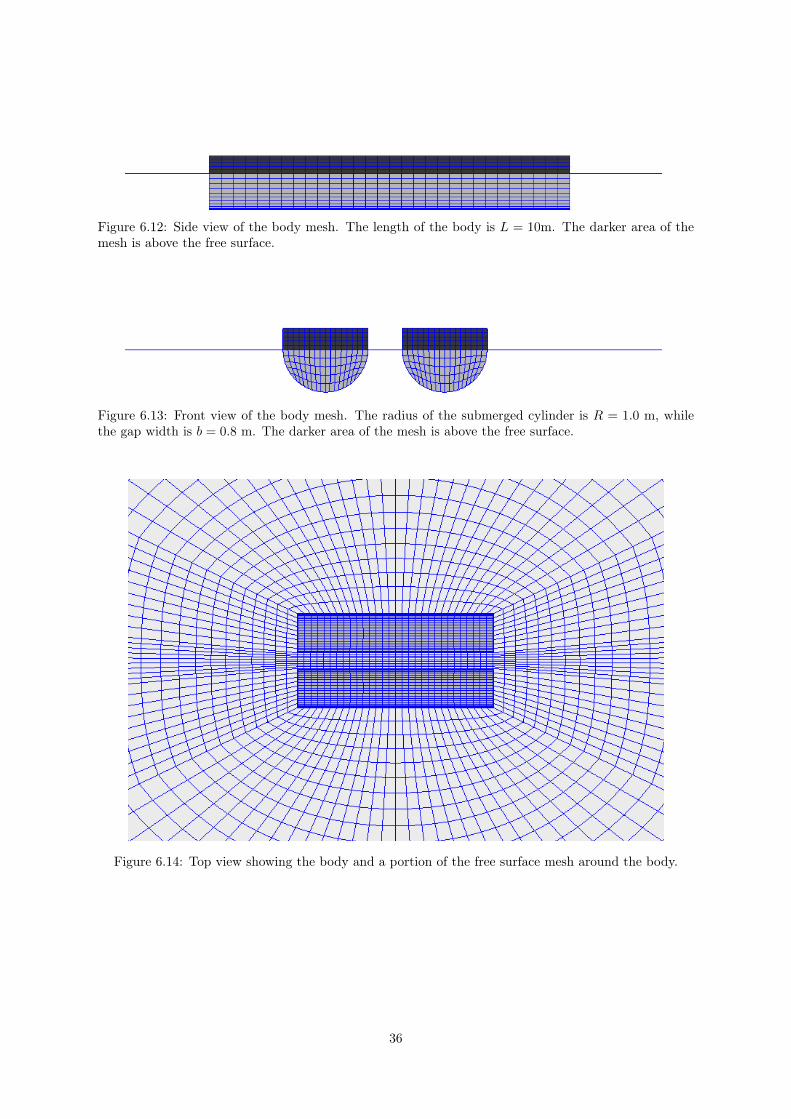
Figure 6.12: Side view of the body mesh. The length of the body is L = 10m. The darker area of themesh is above the free surface.

Figure 6.13: Front view of the body mesh. The radius of the submerged cylinder is R = 1.0 m, whilethe gap width is b = 0.8 m. The darker area of the mesh is above the free surface.

Figure 6.14: Top view showing the body and a portion of the free surface mesh around the body.

36

0 0.5 1 1.5 2 2.50

0.5

1

1.5

2

2.5

3

3.5

4

4.5

5

5.5

ω 2

gR

Ag

A

Wasim (3d)

Present 2d solver

Figure 6.15: Dimensionless wave amplitude at thecenter point of the gap.

0 0.5 1 1.5 2 2.50

0.2

0.4

0.6

0.8

1

1.2

1.4

1.6

1.8

ω 2

gR

|ξ3|

A

Wasim (3d)

Present 2d solver

Figure 6.16: Heave RAO for the pair of circular cylin-der in beam sea.

Figure 6.17: Beam sea with amplitude 0.1m upon rigidly connected cylinders for a given wave frequency.The figure illustrates variations along the gap length which is not present in the two-dimensional case.

37

6.3 Free surface pressure model

6.3.1 Introductory remarksThe wave contribution caused by the free surface pressure will be referred to asthe pressure generated wave in this discussion. The viscous force defined in 3.5will always act in the opposite direction of the fluid velocity in the gap. Whenthe force is represented by a free surface pressure, an equivalent requirement isthat the pressure generated wave contribution must be in opposoite phase ofthe undamped wave. This will not happen if the pressure is given the oppositephase of the fluid velocity. The pressure generated wave will undergo a phaseshift at resonance, just as the undamped wave, so if the pressure is given aphase shift at resonace, the pressure generated wave will experience a doublephase shift. From the following study of forced heave motion we found that thepressure should have the same phase as the body motion to behave correctly atresonance. Figure 6.18 shows the phase angles for the wave trigged by forcedbody motion, the wave generated by the free surface pressure and the total waveconsisting og both contributions. The total wave will have the same phase asthe motion generated wave contribution as long as the amplitude of the pressuregenerated wave is less than the amplitude of the motion generated wave.An other issue is related to the fact that the pressure is non-linear in the am-plitude of the undamped solution in our formulation. In heave motion this mayresult in the behaviour shown in figure 6.19 when the forced motion amplitudeexceeds a certain value. It is our belief that this is unphysical, and that it occurbecause we use the undamped amplitude in the formulation for the pressure.

0.6 0.7 0.8 0.9 1 1.1 1.2 1.3 1.4 1.5 1.6

−3

−2

−1

0

1

2

3

ω 2

gB

θ

Motion generated wave

Pressure generated wave

Pressure damped wave

Figure 6.18: Phase angles for thewave induced by forced body motion,the pressure generated wave and thetotal sum.

0.6 0.7 0.8 0.9 1 1.1 1.2 1.3 1.4 1.5 1.60

2

4

6

8

10

12

14

16

ω 2

gB

No additional damping|ξ

3|/B=0.035

|ξ3|/B=0.045

|ξ3|/B=0.055

Ag/|ξ

3|

Figure 6.19: Local minimum at res-onance may occurs due to that thepressure is non-linear in the ampli-tude of the undamped solution.

38

6.3.2 Heaving of rectangular boxesAs an application of the Pressure Damping Method, we will perform an in-depthanalysis of two closely spaced boxes in forced harmonic heave motion with anoscillating pressure distribution on the gap surface. The pressure distribution isrelated to the viscous forces as in section 4.2. We investigate the local effects inmeans of wave amplitude and phase, force coefficients and gap energy density.The effect in the far-field is investigated through far-field amplitudes and energyflux.Due to the formulation of the pressure amplitude, the pressure damped wavewill be dependent on the amplitude of the heave oscillation. Different heaveamplitudes are considered.We have discussed different sources of viscous damping; skin friction, vortexshedding from corners and bilge keel effects. The analysis will indicate therelative importance of these effects.

Eddy damping

Vortex shedding from the bilge corners is expected to be the most significantviscous effect. We apply the Pressure Damping Model with the pressure dis-tribution in the gap related to the eddy damping discussed in section 3.5.2.The vortex induced damping effect on the piston-like elevation in the gap isdisplayed in figure 6.20 for some given values of the heave amplitude. Far-fieldamplitudes are shown in figure 6.21. Both amplitudes has been reduced dueto the simulated eddy damping. The accompanying added mass and dampingcoefficient are displayed in figure 6.23 and 6.24.We introduce the term relative damping and define it as

∆AgAg0

=Ag0 −AgAg0

, (6.11)

where Ag0 is the amplitude when no additional damping is applied, and Ag is thedamped amplitude. The relative damping is then describing the proportion ofreduction in amplitude, relative to the original amplitude. Figure 6.22 displaysthe relative damping for three different gap lengths, for a continuous variationof the heave amplitude. Note from the figure that the relative damping doesnot have ∆Ag/Ag0 = 1 as a limit when the heave amplitude increases. Whenthe relative damping exceeds 1, the pressure generated wave contribution islarger than the original. The result will be a wave with opposite phase of theoriginal wave. This is of course completely unphysical, and a consequence of theformulation. This suggests that the method is only valid for a range of heaveamplitudes. As discussed in section 6.3.1, applied pressure which result in alocal minimum at resonance is questionable. The dashed lines in figure 6.22indicates where the results tends to exhibit this behaviour.

39

0.6 0.7 0.8 0.9 1 1.1 1.2 1.3 1.4 1.5 1.60

2

4

6

8

10

12

14

16

ω 2

gB

No additional damping|ξ

3|/B=0.015

|ξ3|/B=0.025

|ξ3|/B=0.035

Ag/|ξ

3|

Figure 6.20: Non-dimensional gap amplitude Ag/|ξ3|.B/D = 2, b/D = 1.

0.6 0.7 0.8 0.9 1 1.1 1.2 1.3 1.4 1.5 1.60

0.5

1

1.5

2

2.5

3

ω 2

gB

No additional damping|ξ

3|/B=0.015

|ξ3|/B=0.025

|ξ3|/B=0.035

Af/|ξ

3|

Figure 6.21: Non-dimensional far-field amplitudeAf/|ξ3|. B/D = 2, b/D = 1.

0 0.01 0.02 0.03 0.04 0.05 0.060

0.1

0.2

0.3

0.4

0.5

0.6

0.7

0.8

0.9

1

|ξ3|

B

∆A

g

Ag0

b

D= 1 .0

b

D= 0 .5

b

D= 0 .2

Figure 6.22: Relative damping for three different gap lengths for various values of the heave amplitude. B/D = 2.

40

0.6 0.7 0.8 0.9 1 1.1 1.2 1.3 1.4 1.5 1.6−4

−3

−2

−1

0

1

2

3

ω 2

gB

a33

ρB

2

No additional damping|ξ

3|/B=0.015

|ξ3|/B=0.025

|ξ3|/B=0.035

1.02 1.04 1.06 1.08 1.1 1.12

−3.2

−3.1

−3

−2.9

−2.8

−2.7

−2.6

−2.5

−2.4

Magnified minimum

Figure 6.23: Non-dimensional added mass for different heave amplitudes. B/D = 2, b/D = 1.

0.6 0.7 0.8 0.9 1 1.1 1.2 1.3 1.4 1.5 1.60

0.2

0.4

0.6

0.8

1

1.2

1.4

1.6

1.8

2

ω 2

gB

b33

ρB

2√

gB

No additional damping|ξ

3|/B=0.015

|ξ3|/B=0.025

|ξ3|/B=0.035

0.98 1 1.02 1.04 1.06 1.081.1

1.2

1.3

1.4

1.5

1.6

Magnified maximum

Figure 6.24: Non-dimensional damping coefficient for different heave amplitudes. B/D = 2, b/D = 1.

41

The pressure will do work on the free surface. We can calculate the work doneby the pressure over one cycle as

W = −Fv, (6.12)

where v is the free surface velocity. The energy will be transported away withthe pressure generated waves. We may controll the calculations by the theenergy flux in the far-field given in (6.5). Figure 6.25 displays both the averagework and the average energy flux for three different heave amplitudes. Thepressure force is dependent on the wave amplitude squared, and hence the workgets a cubic dependence. As the pressure force represents the viscous force, andit does work against the free surface motion this could be regarded as energydissipated by viscousity.

0.85 0.9 0.95 1 1.05 1.1 1.15 1.2 1.25

0

0.2

0.4

0.6

0.8

1

1.2

W/(ρBg√

Bg)

ω 2

gB

|ξ3|/B=0.015

|ξ3|/B=0.025

|ξ3|/B=0.035

Figure 6.25: Average work done by the free surface pressure in the gap. Thecircles indicates calculated values for the average far-field energy flux. B/D = 2,b/D = 1.

42

Skin friction

The skin friction effects on the gap wave amplitude is considered. The sameforcing amplitudes as in figure 6.20 are considered to get an impression of the rel-ative importance. Figure 6.26 displays the reduction in wave amplitude aroundthe gap resonance frequency. It is evident that this effect is negligible comparedto effect of vortex shedding. This also implies that the effect of skin frictionhas negligible impact on the hydrodynamic coefficients. Skin friction will notbe considered further.

1.0395 1.04 1.0405 1.041 1.0415 1.042

15.927

15.928

15.929

15.93

15.931

15.932

15.933

15.934

ω 2

gB

No additional damping|ξ

3|/B=0.015

|ξ3|/B=0.025

|ξ3|/B=0.035

Ag/|ξ

3|

Figure 6.26: Effect of skin friction on the piston mode amplitude around the gapresonance frequency. The effect is negligible compared to the effect of vortexshedding. Note the scale on the y-axis. B/D = 2, b/D = 1.

43

Bilge keel effects

The viscous effect associated with bilge keels is considered. This will ultimatelybe an additional effect which adds up to the eddy damping, but here we considerthe individual effect. Two different widths has been tested. Figure 6.27a and6.27b shows the reduction in amplitude due to bilge keels with width Bbk/b = 0.1and Bbk = 0.2, respectively. The length of one keel is 5% of the body width Bin the first case, and 10% for the second. Although more apparent for the largerbilge keels, the effect is small compared to the eddy damping.The pair of bilge keels covers the gap opening by 20% in the first case, and 40%in the second case. This should result in less fluid entering the gap. This hasnot been accounted for, as only the viscous contribution from the bilge keels hasbeen considered. The effect of covering the gap is presumably a potential floweffect, and could be captured by modeling the bilge keels in the panel model.

1.02 1.025 1.03 1.035 1.04 1.045 1.05 1.055 1.06 1.065

15.2

15.4

15.6

15.8

16

16.2

ω 2

gB

No additional damping|ξ

3|/B=0.015

|ξ3|/B=0.025

|ξ3|/B=0.035

Ag/|ξ

3|

(a) Bilge keel width Bbk/b = 0.1.B/D = 2, b/D = 1

1.02 1.025 1.03 1.035 1.04 1.045 1.05 1.055 1.06 1.065

15.2

15.4

15.6

15.8

16

16.2

ω 2

gB

No additional damping|ξ

3|/B=0.015

|ξ3|/B=0.025

|ξ3|/B=0.035

Ag/|ξ

3|

(b) Bilge keel width Bbk/b = 0.2.B/D = 2, b/D = 1

Figure 6.27: Non-dimensional gap amplitude. Viscous effect from bilge keelsare considered.

44

6.4 Newtonian Cooling Damping ModelThe newtonian cooling damping model is applied in the gap. Forced heave mo-tion is considered to obtain comparable results to the Pressure Damping Modelin 6.3. We give the damping paramter ν different values to obtain differentdegree of damped elevation and hydrodynamic coefficients.

6.4.1 Heaving of rectangular boxesThe newtonian cooling damping model is not dependent on the value of theheave amplitude ξ3. The resulting damping depends only on the damping co-efficient ν for a given geometry. Figure 6.28 displays the gap wave amplitude.Figure 6.29 displays the associated far-field aplitudes. A noteworthy occurrencein the far-field takes place around ω2B/g = 1.2, where the basis solution hasits minimum. For the consecutive frequencies, the amplitudes is larger than forthe basis solution. The reason for this is clearfied by the damping coefficient.The added mass and damping coefficient are displayed in 6.31 and 6.32. Weobserve that the overall resonant behaviour is broaden out for increasing valuesof ν. This results in larger damping coefficients in the frequency region afterresonance. The damping is directly related to the far-field waves and hencelarger amplitude is expected. Not much is to say about the Newtonian coolingeffect on the gap wave amplitude, as well as the added mass coefficient. Theirmagnitudes are reduced for increasing values of ν, as expected.The relative damping in the gap is displayd in 6.30, for three different gapwidths. The relative damping has asymptotes ∆Ag/Ag0 = 1. This implies thatthe wave elevation will eventually be damped to zero for larger values of ν. Wealso observes that a smaller value of d/B leads to larger relative damping forany given ν.

Comparison with Wasim

The Newtonian cooling formulation is originally included in Wasim for use innumerical beach context. The formulation may also be applied on areas of thefree surface which is not a part of the numerical beach. Wasim has been usedwith Newtonian cooling in the gap to obtain damped gap wave amplitudes forthe situation discussed in 6.2.4. We compare them to result from our present2D code. As discussed in 6.2.4, 2D and 3D results are not directly comparablemainly due the variation in elevation in the length direction of the gap in 3D.Nevertheless, the peak wave amplitude is of approximately equal value and wewill see how this is affected by the Newtonian cooling damping for some givenν-values. The result is shown in figure 6.33. We observe that the 3D calculationsseems to be slightly more affected by the Newtonian cooling.

45

0.6 0.7 0.8 0.9 1 1.1 1.2 1.3 1.4 1.5 1.60

2

4

6

8

10

12

14

16

ω 2

gB

No additional damping

ν=0.01

ν=0.05

ν=0.10

ν=0.20

Ag/|ξ

3|

Figure 6.28: Non-dimensional gap amplitude.

0.6 0.7 0.8 0.9 1 1.1 1.2 1.3 1.4 1.5 1.60

0.5

1

1.5

2

2.5

3

ω 2

gB

No additional damping

ν=0.01

ν=0.05

ν=0.10

ν=0.20

Af/|ξ

3|

Figure 6.29: Non-dimensional far-field amplitude.

0 0.05 0.1 0.15 0.2 0.25 0.30

0.1

0.2

0.3

0.4

0.5

0.6

0.7

0.8

0.9

1

∆A

g

Ag0

ν

b/D=1.0

b/D=0.5

b/D=0.2

Figure 6.30: Relative damping for three different gap lengths for various values of the damping coefficient. B/D = 2

46

0.6 0.7 0.8 0.9 1 1.1 1.2 1.3 1.4 1.5 1.6−4

−3

−2

−1

0

1

2

3

ω 2

gB

a33

ρB

2

No additional damping

ν=0.01

ν=0.05

ν=0.10

ν=0.20

Figure 6.31: Non-dimensional added mass for different values of ν. B/D = 2, b/D = 1.

0.6 0.7 0.8 0.9 1 1.1 1.2 1.3 1.4 1.5 1.60

0.2

0.4

0.6

0.8

1

1.2

1.4

1.6

1.8

2

ω 2

gB

b33

ρB

2√

gB

No additional damping

ν=0.01

ν=0.05

ν=0.10

ν=0.20

Figure 6.32: Non-dimensional damping coefficient for different values of ν. B/D = 2, b/D = 1.

47

0.9 1 1.1 1.2 1.3 1.4 1.50

0.5

1

1.5

2

2.5

3

3.5

4

4.5

5

5.5

ω 2

gR

Ag

A

Wasim (3d). ν=0.0

Present(2d). ν=0.0

Wasim (3d). ν=0.01

Present(2d). ν=0.01

Wasim (3d). ν=0.05

Present(2d). ν=0.05

Wasim (3d). ν=0.10

Present(2d). ν=0.10

Figure 6.33: Wasim(3D) with Newtonian cooling, compared to present(2D) re-sults. Circular cylinders as in section 6.2.4

48

6.5 Comparison of the damping modelsWe have demonstrated how both the Pressure Damping Method and the Newto-nian Cooling Damping Model provides damping of the heave induced piston-likemotion in the gap. In the Pressure Damping Model we get larger damping effectwhen the forced motion amplitude is increased. This is due to the formelationof the pressure distribution (4.5), which is non-linear in the undamped waveamplitude. The Newtonian Cooling Model is linear and thus not affected by theamplitude of heave motion. Instead we may obtain different degree of damp-ing by varying the damping coefficient ν. It should be repeated that the valueof ν is not related to physics, while the damping effect obtained for a givenheave amplitude is related to the physical viscous effects. The viscous effectsare non-linear, and so it seems questionable to model these effects by the linearNewtonian Cooling Damping Model, unless ν is somehow related to ξ3.Some key results obtained from the analysis in 6.4 and 6.3 are listed in table 6.1and 6.2. For each |ξ3|/B there is a ν which gives the same damped amplitde atresonance. As an example we have shown calculation with |ξ3|/B = 0.031 andν = 0.057 for b/D = 1.0 in figure 6.34. We see that the curves coincides wellfor all displayed frequencies. The reason for the minor discrepancy at the peakis that the values in table 6.1 are rounded.

Relative damping (%)

10% 20% 30% 40%

|ξ3|B

= 0.018|ξ3|B

= 0.025|ξ3|B

= 0.031|ξ3|B

= 0.037

ν = 0.015 ν = 0.034 ν = 0.058 ν = 0.080

Table 6.1: Comparison of the Newtonian cooling damping model and the pres-sure damping model. b/D = 1.0, B/D = 2

Relative damping (%)

10% 20% 30% 40%

|ξ3|B

= 0.009|ξ3|B

= 0.013|ξ3|B

= 0.016|ξ3|B

= 0.017

ν = 0.012 ν = 0.025 ν = 0.045 ν = 0.060

Table 6.2: Comparison of the Newtonian cooling damping model and the pres-sure damping model. b/D = 0.5, B/D = 2

49

0.6 0.7 0.8 0.9 1 1.1 1.2 1.3 1.4 1.5 1.60

2

4

6

8

10

12

14

16

ω 2

gB

No additional damping|ξ

3|/B=0.031

ν=0.057

Ag/|ξ

3|

Figure 6.34: Comparison of the heave generated elevation damped by the twodifferent damping models. The relative damping(%) is 30%. b/D = 1, B/D = 2

50

Chapter 7

Summary and conclusion

The resonant behaviour occuring when a gap is present has been numericallyinvestigated with Boundary Element Method. Empirical formulas for the damp-ing effect of different viscous forces were related to the Pressure Damping Model.By comparing the effect of skin friction and vortex shedding, we conclude thatskin friction is negligible. Viscous effects from bilge keels in the gap were shownto be small compared to the eddy damping. However, the coverage of the gapby the keels were not considered. It is presumable that this is an importanteffect of bilge keels as they prevents as much water to enter the gap. Althoughsome assumptions were made to form simple expressions for the viscous damp-ing, we hope to have captured the leading effects. The procedure of relating theviscous forces to a pressure distribution on the gap surface is general, so anyempirical formulas may be used. We have demonstraded how the NewtonianCooling Damping Model can be compared to the Pressure Damping Model toyield estimates for the Newtonian cooling damping coefficient. If one are ableto get good estimations for the viscous forces, this method could be a simplealternative to CFD analysis or model tests.A three dimensional analysis was carried out using Wasim. In this context three-dimensional flow effects were briefly discussed. We conclude that the analogybetween three-dimensional cylinders and a two-dimensional cross section shouldnot be pushed to far, as longitudinal variations occur in the gap in the three-dimensional case.

51

Appendices

52

Appendix A

Greens theorem

Given the functions f and g defined in Ω, bounded by the boundary δΩ. Greenssecond identity relate the volume integral to a surface integral,

∫Ω

(f∇2g − g∇2f) dV =

∫δΩ

(f∂g

∂n− g ∂f

∂n

)dS. (A.1)

We consider two Laplacian potentials, ϕ and ψ defined in the volume V , withboundary S. It follows from Greens theorem that.

∫S

(ϕ∂ψ

∂n− ψ∂ϕ

∂n

)dS = 0. (A.2)

We let ψ be a source with fieldpoint x and source point ξ. The two dimensionalsource

ψ = ln r (A.3)

where r = |x−ξ| =√

(x− ξ)2 + (z − ζ). When r = 0 then ψ becomes singular,and does not satify ∇2ψ = 0. Except at the singular point the function is Lapla-cian. We enclose the singular point x− ξ by a circle or half circle if x is on thefluid boundary. The contributions from the limits of the circle/halfcircle aroundthe singularity could be found by taylor-expansion. The resulting expression is

∫S

(ϕ(ξ)

∂G(ξ; x)

∂nξ−G(ξ; x)

∂ϕ(ξ)

∂nξ

)dξ =

0, outside the fluid domainπϕ(x), on the boundary2πϕ(x), inside the fluid domain

(A.4)

53

Appendix B

Equivalent linearization

Consider a non-linear force given by

F =1

2ρL2

cCd|v|v

as in 4.2.1, where v = v(t) = V0cos(ωt + θ). The phase θ may be disregardedfor this derivation. We denote the constants as F0 = 1/2ρL2

cCd for simplicity.We seek to find a linear expression on the form

F = KF0v, (B.1)

where K is an unknown constant, so that the work done over one period is thesame for this expression and the non-linear expression.The work done by F over one period is

W =

∫ 2π/ω

0

F0V20 cos(ωt)| cos(ωt)| · V0 cos(ωt) dt

= F08V 3

0

3ω.

(B.2)

The work done by F over one period is

W =

∫ 2π/ω

0

KF0V0 cos(ωt) · V0 cos(ωt) dt

= KF0π

ωV 2

0

(B.3)

The constant K is found by equation W and W ,

KF0π

ωV 2

0 = F08V 3

0

3ω(B.4)

K =8V0

3π(B.5)

The equivalent linearized expression for F is now given as

F ≈ F =8

3πF0V0v

=4

3πρL2

cCdV0v.

(B.6)

54

Appendix C

Convergence test

Convergence of the computed piston mode amplitude is considered. The resultis displayed in figure C.1. The percentage difference for the peak amplitudebetween N = 54 and N = 78 is 1.065%. The percentage difference betweem thefrequencies where peak amplitude occurs for N = 54 and N = 78 is 0.192%.The percentage difference for the peak amplitude between N = 72 and N = 78is 0.18%. A number of N = 72 panels where used throughout the numericalstudy in chapter 6. Percentage difference bewteen two value is given as

∆percentage =|x1 − x2|

(x1 − x2)/2,

where x1 and x2 represents the two values.

1.03 1.035 1.04 1.045 1.0515.65

15.7

15.75

15.8

15.85

15.9

15.95

16

16.05

16.1

ω 2

gB

Ag/|

ξ 3|

N=54

N=60

N=72

N=78

Figure C.1: Results from convergence test. Nondimensional piston mode am-plitude Ag/|ξ3| for different number of panels. Note the axes.

55

Appendix D

Equation of motion

Motions in two dimensions are considered, with i, j = 2, 3, 4 representing sway,heave and roll respectively. The equation of motion for a freely floating bodyfollows from Newton’s second law,

Fi =

4∑j=2

MijUj i, j = 2, 3, 4. (D.1)

The body acceleration is given as

Uj = Re−ω2ξjeiωt i, j = 2, 3, 4. (D.2)

The product MijUj is the body inertia forces. The mass matrix Mij for ourtwo-dimensional problem is given as

Mij =

m 0 0

0 m 0

0 0 I11

(D.3)

with the body mass as the displaced water volume times the density

m = ρV (D.4)

and the roll moment of inertia

I11 =

∫∫ρB(x · x− x2

1) dV. (D.5)

The inertia forces equals the forces which acting on the body. We have definedthe force due to body motion in (6.1), and the force from the incident wavein (6.7). In addition to these force components we have the restoring force.The restoring force is zero for sway motion, while heave and roll restoring forcecoefficients are given as

c33 = ρgS (D.6)

c44 = ρgV [S22

V+ yB − yG] (D.7)

56

with S22 as the waterplane moment, and yB and yG is the center of bouyancyand the center of gravity. The total restoring force is proportional to ξj . As allforces are varying with as eiωt we may omit the factor and express the equationof motion through the added mass and damping coefficient (6.3), restoring forcecoefficient (D.6) and the excitation force coefficients (6.8),

4∑j=1

ξj(−ω2(Mij + aij) + iωbij + cij) = AXi (D.8)

for i, j = 2, 3, 4.

57

Bibliography

[1] Bearman P.W. Vortex Shedding From Oscillating Bluff-Bodies. Annual Re-view of Fluic Mechanics 1984;vol16:195–222

[2] Buchner B, Van Dijk A, De Wilde J. Numerical Multiple-Body Simulationsof Side-by-Side Mooring to an FPSO. Proc. of IOPEC2001.

[3] Chen X., Duan W. Multi-domain Boundary Element Method with Dissipa-tion. Journal of Marine Science and Applications 2012;11:18–23

[4] Faltinsen O.M. Resonant liquid motion in marine hydrodynamics. ProcediaEngineering 2015;126:6–11

[5] Heo JK, Park JC, Koo WC, Kim MH. Influences of Vorticity to VerticalMotion of Two-Dimensional Moonpool under Forced Heave Motion. Math-ematical Problems in Engineering Volume 2014

[6] Israeli M, Orszag S.A. Approximation of Radiation Boundary Conditions.Journal of Computational Physics 1981;41:115–135

[7] Kristiansen T, Faltinsen O.M. A two-dimensional numerical and experi-mental study of resonant coupled ship and piston-mode motion. Appliedocean Reasearch 2012;32:158–176

[8] Kristiansen T., Faltinsen O.M. Gap resonance analyzed by a domain-decomosition method combining potential and viscous flow DRAFT. Ap-plied Ocean Research 2012;34:198–208

[9] Molin B. On the piston mode in moonpools. Proc. 14th Int. Workshop onWater Waves & Floating Bodies Port Huron, 1999

[10] Newman J.N. Marine Hydrodynamics, MIT Press 1977.

[11] Newman J.N. Progress in wave load computations on offshore structures.Proc 23th OMAE, Vancouver, Canada, 2004.

[12] Lee, C.-H. and Nielsen, F.G Analysis of oscillating-water column deviceusing a panel method., presented at 11th International Workshop on WaterWaves and Floating Bodies, Hamburg , 1996

[13] Ogilvie TF. Oscillating Pressure Field on A Free Surface. 1969

[14] Sun L, Taylor P. First- and second order analysis of resonant waves betweenadjacent barges. Journal of Fluids and Structures 2010

58

[15] Wang H, Falzarano JM. Energy extraction from the motion of an oscillatingwater column. Oscean System Engineering 2013;vol3:327–348

[16] Wehausen J.V, Laitone E. V. Surface waves. Handbuch der Physics1960;Vol. 9

59