investigation of in-situ combustion kinetics using the ...mf038wz2108/... · and the measured data...
TRANSCRIPT

INVESTIGATION OF IN-SITU COMBUSTION KINETICS
USING THE ISOCONVERSIONAL PRINCIPLE
A DISSERTATION
SUBMITTED TO THE DEPARTMENT OF ENERGY
RESOURCES ENGINEERING
AND THE COMMITTEE ON GRADUATE STUDIES
OF STANFORD UNIVERSITY
IN PARTIAL FULFILLMENT OF THE REQUIREMENTS
FOR THE DEGREE OF
DOCTOR OF PHILOSOPHY
Bo Chen
November 2012

http://creativecommons.org/licenses/by-nc/3.0/us/
This dissertation is online at: http://purl.stanford.edu/mf038wz2108
© 2012 by Bo Chen. All Rights Reserved.
Re-distributed by Stanford University under license with the author.
This work is licensed under a Creative Commons Attribution-Noncommercial 3.0 United States License.
ii

I certify that I have read this dissertation and that, in my opinion, it is fully adequatein scope and quality as a dissertation for the degree of Doctor of Philosophy.
Anthony Kovscek, Primary Adviser
I certify that I have read this dissertation and that, in my opinion, it is fully adequatein scope and quality as a dissertation for the degree of Doctor of Philosophy.
Louis Castanier
I certify that I have read this dissertation and that, in my opinion, it is fully adequatein scope and quality as a dissertation for the degree of Doctor of Philosophy.
Margot Gerritsen
Approved for the Stanford University Committee on Graduate Studies.
Patricia J. Gumport, Vice Provost Graduate Education
This signature page was generated electronically upon submission of this dissertation in electronic format. An original signed hard copy of the signature page is on file inUniversity Archives.
iii

Abstract
In-situ combustion (ISC) is the most energy efficient thermal enhanced oil recovery
(EOR) method implemented in crude-oil reservoirs. The worldwide implementation
of ISC in commercial field projects reached a maximum of 19 during the period of
1970’s to 1990’s, but it has declined to 4 active operations nowadays. Many failed
projects are due to incorrect operations. Understanding the complicated combustion
kinetics during the ISC process is essential and significantly important to optimize
field operation.
The combination of the experimental tool, ramped temperature oxidation (RTO),
and the measured data interpretation method, isoconversional principle, provides a
workflow to unlock the complicated characteristics of ISC kinetics. Conducting reli-
able or repeatable RTO experiments for isoconversional interpretation is the baseline
for the workflow. Simulations coupled with a synthetic reaction model in an in-
house virtual kinetic cell (VKC) simulator show that reducing temperature deviation
caused by exothermic reactions is critical to carry out consistent RTO experiments.
The argument is supported by a series of RTO experiments of the same crude-oil
mixture, but different working conditions with respect to the kinetic cell design, the
volumetric flow rate of air injection and the size of the sample mixture. Further-
more, the consistent RTO experimental results prove the model-free nature of the
isoconversional principle and its applicability in the investigation of ISC kinetics. An
attempt to combine the isoconversional principle and the conventional interpretation
method is proposed to interpret kinetic parameters including apparent activation
energy, pre-exponential factor and reaction orders for both fuel and oxygen partial
pressure. Simulations in the VKC were carried out to test the proposed method for
iv
a unit and a non-unit reaction order case. The result showed good matches in the
kinetic parameters between the interpretation and the simulations. A three-reaction
scheme is proposed for two crude-oil mixtures, Alaska crude-oil and Karamay crude-
oil, based on the observation and analysis of the activation energy fingerprints and the
effluent data. The stoichiometry and the kinetic parameters for the reaction model
are interpreted by the proposed method. The combustion models are verified in the
commercial reservoir simulator CMG-STARS regarding the temperature histories, the
effluent data from RTO experiments, and the isoconversional fingerprints. Further
application of the isoconversional principle to analyze the crude-oil combustion in-
cludes investigating the sand and clay surface effect on the reaction paths together
with X-ray photoelectron spectroscopy (XPS) to study the coke formation charac-
teristics and their reaction kinetics. Screening the ISC candidates with respect to
different crude-oil/sand-matrix pairs is also discussed. Lastly, the development of a
microwave heating system is discussed to replace the conventional electric furnace
system to carry out RTO experiments. Three generations of the microwave heating
system are developed and discussed.
v

Acknowledgements
As my wife and friends always say I am a lucky person, this is really the truth
when I gained the opportunity to be a PhD student in Professor Anthony Kovscek’s
group. I will never ever forget every moment I entered Professor Kovscek’s office with
discouraging results from my research, I always received encouraging words and warm
smiles from him even if he was busy with his work. I sincerely appreciate all of the
knowledge and skills I have learned during my PhD course under Professor Kovscek’s
supervision. Meanwhile, I feel guilty I should have contributed more to this exciting
group, SUPRI-A.
Sincere thanks are given to Dr. Louis Castanier for his great help to my research.
I can remember every time I knocked at the door of his office, saying ’good morning
Louis’, there is always a happy response from inside ’just a sec...’ Sincere thanks
are also due to Professor Margot Gerritsen, Professor Roland Horne and Professor
Jonathan F. Stebbins for serving on the committee. Special thanks are given to ERE
staff, Yolanda D. Williams and Joanna Sun.
My PhD research can not be finished without great help and supports from group
mates and friends. It is my great happiness and gratitude to work with and to be
friend with: Murat Cinar, Yangyang Liu, Mohammad Bazargan, Guenther Glatz,
Berna Hascakir, Alexandre Lapene, Bolivia Vega, Zhouyuan Zhu, Qing Chen, Yang
Liu, Saman Aryana, Egill Juliusson, David Cameron.
I would like to record my gratefulness here to my beloved wife, Xi Wang. She is
the love and happiness to my life, giving me unconditional support to my career. Also
thankfulness is due to my parents and family for their always being there in every
aspect of my life.
vi

Contents
Abstract iv
Acknowledgements vi
1 Introduction 1
1.1 Petroleum overview . . . . . . . . . . . . . . . . . . . . . . . . . . . . 1
1.2 In-situ combustion . . . . . . . . . . . . . . . . . . . . . . . . . . . . 2
1.3 Combustion kinetics . . . . . . . . . . . . . . . . . . . . . . . . . . . 5
1.4 Statement of the problem . . . . . . . . . . . . . . . . . . . . . . . . 7
1.5 Thesis overview . . . . . . . . . . . . . . . . . . . . . . . . . . . . . . 8
2 Consistent RTO experiments and interpretation 12
2.1 Isoconversional principle . . . . . . . . . . . . . . . . . . . . . . . . . 13
2.2 RTO experimental platform and simulator . . . . . . . . . . . . . . . 15
2.3 Consistency . . . . . . . . . . . . . . . . . . . . . . . . . . . . . . . . 18
2.3.1 RTO simulations . . . . . . . . . . . . . . . . . . . . . . . . . 18
2.3.2 RTO experiments . . . . . . . . . . . . . . . . . . . . . . . . . 20
2.4 Repeatable RTO measurements . . . . . . . . . . . . . . . . . . . . . 24
2.5 Conclusion . . . . . . . . . . . . . . . . . . . . . . . . . . . . . . . . . 30
3 Isoconversional modeling and simulation 32
3.1 Defining kinetic parameters . . . . . . . . . . . . . . . . . . . . . . . 34
3.1.1 Defining activation energy . . . . . . . . . . . . . . . . . . . . 37
3.1.2 Defining reaction orders . . . . . . . . . . . . . . . . . . . . . 38
vii

3.1.3 Defining pre-exponential factor . . . . . . . . . . . . . . . . . 39
3.2 Kinetic interpretation for synthetic cases . . . . . . . . . . . . . . . . 39
3.2.1 Synthetic case of unit reaction orders . . . . . . . . . . . . . . 40
3.2.2 Synthetic case of non-unit reaction orders . . . . . . . . . . . 41
3.2.3 Discussion . . . . . . . . . . . . . . . . . . . . . . . . . . . . . 49
3.3 Kinetic interpretation and simulation . . . . . . . . . . . . . . . . . . 49
3.3.1 Gridding strategy . . . . . . . . . . . . . . . . . . . . . . . . . 49
3.3.2 Kinetic reaction scheme . . . . . . . . . . . . . . . . . . . . . 50
3.3.3 Alaskan oil sample . . . . . . . . . . . . . . . . . . . . . . . . 54
3.3.4 Karamay oil sample . . . . . . . . . . . . . . . . . . . . . . . . 62
3.4 Discussion . . . . . . . . . . . . . . . . . . . . . . . . . . . . . . . . . 69
4 Isoconversional application 74
4.1 Reservoir matrix effect . . . . . . . . . . . . . . . . . . . . . . . . . . 74
4.1.1 Alaskan crude-oil cases . . . . . . . . . . . . . . . . . . . . . . 75
4.1.2 Karamay crude-oil cases . . . . . . . . . . . . . . . . . . . . . 81
4.2 Coke formation investigation . . . . . . . . . . . . . . . . . . . . . . . 87
4.2.1 Coke formed under air . . . . . . . . . . . . . . . . . . . . . . 88
4.2.2 Coke formed under nitrogen . . . . . . . . . . . . . . . . . . . 94
4.2.3 XPS analysis . . . . . . . . . . . . . . . . . . . . . . . . . . . 95
4.3 ISC candidate screening . . . . . . . . . . . . . . . . . . . . . . . . . 98
5 RTO kinetics using electromagnetic radiation 107
5.1 Literature review . . . . . . . . . . . . . . . . . . . . . . . . . . . . . 111
5.1.1 Microwave heating effect . . . . . . . . . . . . . . . . . . . . . 111
5.1.2 Temperature measurement . . . . . . . . . . . . . . . . . . . . 113
5.1.3 Microwave heating system . . . . . . . . . . . . . . . . . . . . 115
5.2 Development of microwave heating systems . . . . . . . . . . . . . . . 117
5.2.1 1st generation reactor and embodiments . . . . . . . . . . . . 117
5.2.2 2nd generation reactor and embodiments . . . . . . . . . . . . 121
5.2.3 3rd generation reactor and embodiments . . . . . . . . . . . . 126
5.2.4 Parallel electromagnetic heating system . . . . . . . . . . . . . 133
viii

5.3 Discussion . . . . . . . . . . . . . . . . . . . . . . . . . . . . . . . . . 135
6 Summary and discussion 139
A Updates for the kinetic cell and combustion tube systems 143
B Background correction of effluent data 146
C Kinetic cell experiment preparation 150
D Codes for virtual kinetic cell simulation and isoconversional inter-
pretation 152
E Input file of kinetic cell simulation for CMG-STARS 169
Bibliography 187
ix

List of Tables
2.1 Kinetic cell designs . . . . . . . . . . . . . . . . . . . . . . . . . . . . 16
2.2 Arrhenius parameters for the synthetic model . . . . . . . . . . . . . 18
2.3 Heat of reaction values for different simulation cases . . . . . . . . . . 20
3.1 Arrhenius parameters used in the synthetic case of unit reaction orders 41
3.2 Error analysis for the synthetic case of unit reaction orders . . . . . . 45
3.3 Arrhenius parameters used in the synthetic case of non-unit reaction
orders . . . . . . . . . . . . . . . . . . . . . . . . . . . . . . . . . . . 45
3.4 Error analysis for the non-unit reaction order case . . . . . . . . . . . 45
3.5 Comparison between initial and adjusted values of pre-exponential fac-
tor for the Alaska crude-oil combustion modeling. . . . . . . . . . . . 62
3.6 Kinetic parameters for the proposed model of the Alaska crude-oil com-
bustion. . . . . . . . . . . . . . . . . . . . . . . . . . . . . . . . . . . 62
3.7 Kinetic parameters for proposed model of the Karamay crude-oil com-
bustion . . . . . . . . . . . . . . . . . . . . . . . . . . . . . . . . . . . 64
4.1 Crude-oil/rock matrix pairs for RTO experiments . . . . . . . . . . . 75
4.2 Oxygen consumption comparison of LTO and HTO for Alaskan crude
oil cases . . . . . . . . . . . . . . . . . . . . . . . . . . . . . . . . . . 76
4.3 Oxygen consumption comparison of LTO and HTO for Karamay crude
oil cases . . . . . . . . . . . . . . . . . . . . . . . . . . . . . . . . . . 82
4.4 Oxygen carbon ratios on the surface of different coke under air and
nitrogen. . . . . . . . . . . . . . . . . . . . . . . . . . . . . . . . . . . 98
x

5.1 Comparison between microwave heating and furnace heating . . . . . 110
5.2 Experimental conditions . . . . . . . . . . . . . . . . . . . . . . . . . 121
A.1 Mass flow controller calibration table for air . . . . . . . . . . . . . . 144
A.2 Thermocouple enumeration for the kinetic cell system . . . . . . . . . 144
A.3 Thermocouple enumeration for the combustion tube . . . . . . . . . . 145
xi

List of Figures
1.1 In-situ combustion mechanism: (a), Schematic cartoon of a in-situ
combustion process: heat is used to thin the oil and permit it to flow
more easily toward production wells; in a fireflood, the formation is ig-
nited, and by continued injection of air, a fire front is advanced through
the reservoir; the mobility of oil is increased by reduced viscosity caused
by heat and solution of combustion gases. (b), Illustration of tempera-
ture and saturation profiles in a typical in-situ combustion process: ¬
Injected Air and water zone (burned out); Air and vaporized water
zone; ® Burning front and combustion zone (600 - 1200 ◦F ; ¯ Coking
zone; ° Steam or vaporizing zone (Approx. 400 ◦F ; ± Condensing or
hot water zone (50 - 200 ◦F above initial temperature); ² Oil bank
(near initial temperature); ³ Cold combustion gases. . . . . . . . . . 11
2.1 Schematic diagram of RTO platform [17]: ¬ gas tank, mass flow
controller, ® electric furnace, ¯ kinetic cell, ° thermocouple, ± back
pressure controller, ² gas analyzer, ³ computer. . . . . . . . . . . . . 16
2.2 Temperature profiles for the small temperature deviation (STD) case.
For each temperature profile, the first hump represents the low tem-
perature oxidation stage and the second hump represents the high tem-
perature oxidation stage. . . . . . . . . . . . . . . . . . . . . . . . . . 21
xii

2.3 O2 consumption profiles for the small temperature deviation (STD)
case. For each O2 curve, the first hump represents the low temperature
oxidation stage and the second hump represents the high temperature
oxidation stage. The valley between the two stages is the transition
zone. . . . . . . . . . . . . . . . . . . . . . . . . . . . . . . . . . . . . 21
2.4 Temperature versus conversion for the small temperature deviation
(STD) case. The curve of large heat rate is over the one of low heat
rate. There is no intersection between different curves. . . . . . . . . 22
2.5 A plot of ln(d[X]/dt) versus −1/(RT ) for consistency check. The black
solid lines connect dots of the same conversion X of different heat
rates. Trends of each line are linear indication consistency. The slope
represents the apparent activation energy at that conversion X. . . . 22
2.6 Activation energy fingerprints interpreted from the linear temperature
(LT) case, the small temperature deviation (STD) case and the large
temperature deviation (LTD) case using the integral isoconversional
method. . . . . . . . . . . . . . . . . . . . . . . . . . . . . . . . . . . 23
2.7 Temperature histories for the RTO of Alaskan sample mixture: 13.3◦API, 45 grams of the sample mixture are used for each RTO experi-
ment. . . . . . . . . . . . . . . . . . . . . . . . . . . . . . . . . . . . . 24
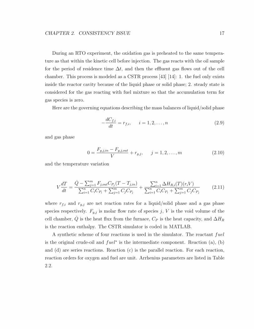
2.8 O2 consumption histories for the RTO of Alaskan sample mixture: 13.3◦API, 45 grams of the sample mixture are used for each RTO experi-
ment. . . . . . . . . . . . . . . . . . . . . . . . . . . . . . . . . . . . . 25
2.9 Temperature versus conversion for the RTO of Alaskan sample mixture:
13.3 ◦API, 45 grams of the sample mixture are used for each RTO
experiment. . . . . . . . . . . . . . . . . . . . . . . . . . . . . . . . . 25
2.10 A plot of ln(d[X]/dt) versus −1/(RT ) for consistency check. The black
solid lines connect dots of the same conversion X of different heat
rates. Trends of each line are not linear for this measurement indicating
inconsistent data. Alaskan sample mixture: 13.3 ◦API, 45 grams of
the sample mixture are used for each RTO experiment. . . . . . . . . 26
xiii

2.11 Apparent activation energy fingerprint obtained from inconsistent data
for the RTO of Alaskan sample mixture: 13.3 ◦API, 45 grams of the
sample mixture are used for each RTO experiment. . . . . . . . . . . 26
2.12 Temperature histories for the RTO of Alaskan sample mixture: 13.3◦API, 25 grams of the sample mixture are used for each RTO experi-
ment. . . . . . . . . . . . . . . . . . . . . . . . . . . . . . . . . . . . . 27
2.13 O2 consumption histories for the RTO of Alaskan sample mixture: 13.3◦API, 25 grams of the sample mixture are used for each RTO experi-
ment. . . . . . . . . . . . . . . . . . . . . . . . . . . . . . . . . . . . . 27
2.14 Temperature versus conversion for the RTO of Alaskan sample mixture:
13.3 ◦API, 25 grams of the sample mixture are used for each RTO
experiment. . . . . . . . . . . . . . . . . . . . . . . . . . . . . . . . . 28
2.15 A plot of ln(d[X]/dt) versus −1/(RT ) for consistency check. The black
solid lines connect dots of the same conversion X of different heat rates.
Trends of each line are linear for this measurement. Alaskan sample
mixture: 13.3 ◦API, 25 grams of the sample mixture are used for each
RTO experiment. . . . . . . . . . . . . . . . . . . . . . . . . . . . . . 28
2.16 Apparent activation energy fingerprint obtained from consistent data
for the RTO of Alaskan sample mixture: 13.3 ◦API, 25 grams of the
sample mixture are used for each RTO experiment. . . . . . . . . . . 29
2.17 Activation energy fingerprints for three cases with different sample
mass of identical composition. Case 1: KC1 is used, 18 grams of
the mixture is used and air injection rate is 1 L/min; Case 2: KC2
is used, 25 grams of the mixture is used and air injection rate is 1.5
L/min; Case 3: KC3 is used, 10 grams, of the mixture is used and air
injection rate is 1 L/min . . . . . . . . . . . . . . . . . . . . . . . . . 30
3.1 Ramped temperature oxidation measurement data . . . . . . . . . . . 35
3.2 Continuous flow reaction process during RTO . . . . . . . . . . . . . 37
3.3 Simulation results for the synthetic case of unit reaction orders: 80%
oxygen in the injection gas stream. . . . . . . . . . . . . . . . . . . . 42
xiv

3.4 Simulation results for the synthetic case of unit reaction orders: 100%
oxygen in the injection gas stream. . . . . . . . . . . . . . . . . . . . 43
3.5 Activation energy fingerprints for unit reaction order cases of different
oxygen compositions in the injection stream: both cases reveal similar
fingerprints because of the identical reaction scheme. . . . . . . . . . 44
3.6 Simulation results for the synthetic case of non-unit reaction orders:
80% oxygen in the injection gas stream. . . . . . . . . . . . . . . . . . 46
3.7 Simulation results for the synthetic case of non-unit reaction orders:
100% oxygen in the injection gas stream. . . . . . . . . . . . . . . . . 47
3.8 Activation energy fingerprints for non-unit reaction order cases of dif-
ferent oxygen compositions in the injection stream: both cases reveal
similar fingerprints because of the identical reaction scheme. . . . . . 48
3.9 Radial griding strategy (4×1×7 for r×θ×h) to mimic the kinetic cell
system in CMG-STARTS (the kinetic cell/furnace schematic diagram
is adapted from a figure in Cinar’s thesis [17]. . . . . . . . . . . . . . 51
3.10 RTO measured effluent data to identify reaction stages, CO2/CO and
O2/CO. . . . . . . . . . . . . . . . . . . . . . . . . . . . . . . . . . . 57
3.11 Isoconversional fingerprints for the four set of RTO experiments using
different oxygen compositions in injection gas stream. The 35% oxygen
case does not show consistent behavior as the other three cases. It is
not used for the oxygen reaction order interpretation. . . . . . . . . . 58
3.12 VKC simulation results based on the initial interpretation for values
of activation energy, reaction orders, and pre-exponential factors A. . 59
3.13 VKC simulation results based on the adjusted pre-exponential factors
A. Interpreted values of activation energies, reaction orders, and stoi-
chiometry are kept the same as those in the initial interpretation sim-
ulation case. The heat rate is 1.85 K/min. . . . . . . . . . . . . . . . 60
3.14 Temperature history comparison between the VKC simulation result
RTO measurement. The heat rate is 1.85 K/min . . . . . . . . . . . 61
3.15 Isoconversional fingerprint comparison between the VKC simulation
result and RTO measurement. . . . . . . . . . . . . . . . . . . . . . . 61
xv

3.16 RTO measured effluent data to identify reaction stages, CO2/CO and
O2/CO. . . . . . . . . . . . . . . . . . . . . . . . . . . . . . . . . . . 65
3.17 Isoconversional fingerprints for the three set of RTO experiments using
different oxygen compositions in the injection gas stream. The 35%
oxygen case does not show consistent behavior as the other three cases.
It is not used for the oxygen reaction order interpretation. . . . . . . 66
3.18 VKC simulation results based on the adjusted pre-exponential factors
A. Interpreted values of activation energies, reaction orders, and stoi-
chiometry are kept the same as those in the initial interpretations: The
heat rate is 1.85 K/min. . . . . . . . . . . . . . . . . . . . . . . . . . 67
3.19 Temperature history comparison between the VKC simulation result
RTO measurement: the heat rate is 1.85 K/min . . . . . . . . . . . . 68
3.20 Isoconversional fingerprint comparison between the VKC simulation
result RTO measurement. . . . . . . . . . . . . . . . . . . . . . . . . 68
3.21 Alaskan crude oil RTO experiments: 35% oxygen composition. . . . . 71
3.22 Karamay crude oil RTO experiments: 35% oxygen composition. . . . 72
3.23 Consistency check for the 35% oxygen composition RTO experiments
of Alaskan crude oil. . . . . . . . . . . . . . . . . . . . . . . . . . . . 73
3.24 Consistency check for the 35% oxygen composition RTO experiments
of Karamay crude oil. . . . . . . . . . . . . . . . . . . . . . . . . . . . 73
4.1 Alaskan crude oil case 1: 60 mesh fired sand and clay; 25g mixture of
2.04 wt% crude oil, 8.16 wt% water, 81.63 wt% fired sand and 8.16
wt% clay; Air injection rate is 1.5 L/min. . . . . . . . . . . . . . . . 77
4.2 Alaskan crude oil case 2: 60 mesh fired sand; 25g mixture of 2.04 wt%
crude oil, 8.16 wt% water, 89.90 wt% fired sand; Air injection rate is
1.5 L/min. . . . . . . . . . . . . . . . . . . . . . . . . . . . . . . . . 78
4.3 Alaskan crude oil case 3: 12 mesh fired sand; 25g mixture of 2.04 wt%
crude oil, 8.16 wt% water, 89.90 wt% fired sand; Air injection rate is
1.5 L/min. . . . . . . . . . . . . . . . . . . . . . . . . . . . . . . . . 79
4.4 Activation energy fingerprints comparison for Alaskan crude oil cases. 81
xvi

4.5 Karamay crude oil case 1: reservoir sand; 15g mixture of 2.04 wt%
crude oil, 8.16 wt% water, 89.90 wt% fired sand; Air injection rate is
1.5 L/min. . . . . . . . . . . . . . . . . . . . . . . . . . . . . . . . . 83
4.6 Karamay crude oil case 2: 60 mesh fired sand and clay; 25g mixture
of 2.04 wt% crude oil, 8.16 wt% water, 81.63 wt% fired sand and 8.16
wt% clay; Air injection rate is 1.5 L/min. . . . . . . . . . . . . . . . 84
4.7 Karamay crude oil case 3: 60 mesh fired sand; 25g mixture of 2.04 wt%
crude oil, 8.16 wt% water, 89.90 wt% fired sand; Air injection rate is
1.5 L/min. . . . . . . . . . . . . . . . . . . . . . . . . . . . . . . . . 85
4.8 Activation energy fingerprints comparison for Karamay crude oil cases. 86
4.9 The kinetic cell for coke formation study in the isothermal condition. 89
4.10 Defining the termination temperature for the isothermal experiment of
air coke formation: 300 ◦C is selected. . . . . . . . . . . . . . . . . . 90
4.11 Coke is formed in the isothermal experiments. . . . . . . . . . . . . . 91
4.12 RTO experiments for the Karamay air coke. . . . . . . . . . . . . . . 92
4.13 Comparison between the activation energy fingerprints for Karamay
air coke and crude oil combustion: the activation energy values on
fingerprint of air coke are very close to the values of HTO region on
the fingerprint of crude oil. . . . . . . . . . . . . . . . . . . . . . . . . 93
4.14 Defining the termination temperature for the isothermal experiment of
N2 coke formation: 420 ◦C is selected. . . . . . . . . . . . . . . . . . 95
4.15 RTO experiments for the Karamay N2 coke . . . . . . . . . . . . . . 96
4.16 Activation energy fingerprint for Karamay N2 coke . . . . . . . . . . 97
4.17 XPS survey spectra of coke formation under air flow condition. Four
spots are scanned. . . . . . . . . . . . . . . . . . . . . . . . . . . . . . 99
4.18 XPS survey spectra of coke formation under nitrogen flow condition.
Four spots are scanned. . . . . . . . . . . . . . . . . . . . . . . . . . . 100
4.19 High resolution XPS C 1s spectra of coke samples precipitated under
air and nitrogen flow conditions . . . . . . . . . . . . . . . . . . . . . 101
4.20 Unsuccessful combustion front propagation: (left) Combustion tube
temperature profile and (right) isoconversional fingerprint [17]. . . . . 102
xvii

4.21 Alaska crude oil combustion tube test with 60 mesh sand and clay. . . 104
4.22 Alaska crude oil combustion tube test with 60 mesh sand. . . . . . . . 105
4.23 Karamay crude oil combustion tube test with reservoir sand. . . . . . 106
5.1 Schematic diagram of microwave heating mechanisms: dipolar polar-
ization and ionic conduction [26]. . . . . . . . . . . . . . . . . . . . . 109
5.2 Temperature distribution difference between conventional and microwave
heating [57]. . . . . . . . . . . . . . . . . . . . . . . . . . . . . . . . . 110
5.3 Temperature (T), pressure (p), and power (P) profile for a 3 mL sample
of methanol heated under sealed vessel single-mode microwave irradi-
ation conditions to 165◦C (external infrared temperature monitoring)
[57]. . . . . . . . . . . . . . . . . . . . . . . . . . . . . . . . . . . . . 116
5.4 Prototype of the 1st generation microwave heating system. The quartz
tube reactor is hung inside the microwave oven cavity. . . . . . . . . . 118
5.5 Metallic cap on the top of the microwave oven. A thermocouple is
inserted through the cap. There are two connectors for injection and
production gas respectively. The cap needs to be well grounded. . . . 118
5.6 Insulation material and its embodiment around the quartz tube reac-
tor: during an experiment, crude oil sample is put at the bottom of the
quartz cell. The body of the tube is wrapped by insulation material
that is transparent to microwave, reducing heat loss to the oven cavity. 119
5.7 Shielded thermocouple and sintered SiC cylinders: sintered SiC cylin-
ders are mixed with crude oil sample, acting as energy absorber to
assist fast heating. . . . . . . . . . . . . . . . . . . . . . . . . . . . . 119
5.8 Schematic diagram of grounded circuit of a shield thermocouple. . . . 120
5.9 Experiment 1: effluent gas histories, 1st generation system. . . . . . . 122
5.10 Experiment 1: temperature profile, 1st generation system. . . . . . . 122
5.11 Experiment 2: temperature profile, 1st generation system. . . . . . . 123
5.12 Schematic design of the 2nd generation reactor. . . . . . . . . . . . . 125
5.13 The reactor embodiment based on a microwave oven. . . . . . . . . . 126
5.14 The prototype of the 2nd generation microwave reactor. . . . . . . . . 127
xviii

5.15 The embodiment in a household microwave oven. . . . . . . . . . . . 127
5.16 Shielded thermocouple and product filter connecter. . . . . . . . . . . 128
5.17 2nd generation microwave heating system. . . . . . . . . . . . . . . . 128
5.18 Schematic design of the 3rd generation reactor. . . . . . . . . . . . . 130
5.19 The prototype of the 3rd generation microwave reactor. . . . . . . . . 131
5.20 The embodiment in a household microwave oven, sintered SiC tube. . 132
5.21 The embodiment in a household microwave oven, sealing cap and
quartz tube. . . . . . . . . . . . . . . . . . . . . . . . . . . . . . . . . 132
5.22 thermocouple and product filter connecter. . . . . . . . . . . . . . . . 133
5.23 Temperature profile of microwave heating of test 1, 3rd generation
system. . . . . . . . . . . . . . . . . . . . . . . . . . . . . . . . . . . . 134
5.24 Temperature profile of microwave heating of test 2, 3rd generation
system. . . . . . . . . . . . . . . . . . . . . . . . . . . . . . . . . . . . 134
5.25 Reactors based on microwave waveguides in a parallel manipulation. . 135
5.26 Schematic of reactor heated by RF radiation. . . . . . . . . . . . . . . 136
5.27 Induction heating with separate attenuator to achieve parallel heating. 137
5.28 Induction heating with different masses of RF absorber to achieve par-
allel heating. . . . . . . . . . . . . . . . . . . . . . . . . . . . . . . . . 137
B.1 Temperature histories for RTO experiments. . . . . . . . . . . . . . . 148
B.2 . . . . . . . . . . . . . . . . . . . . . . . . . . . . . . . . . . . . . . . 149
xix

Chapter 1
Introduction
1.1 Petroleum overview
Petroleum resources are categorized into conventional and unconventional resources.
Conventional crude-oil is easier to recover and the reserves are estimated at around
3,012 billion barrels [126], over 50 percent of which resides in the Middle East.
Roughly, 20-40% of the original oil in place (OOIP) of the conventional crude-oil is
recoverable by primary and secondary processes. When using enhanced oil recovery
(EOR) methods, 30-60% or more of the original oil in reservoir is produced. Technolo-
gies for conventional oil recovery have been well developed for many decades. Their
field implementations are mature and economical. There have been some pessimists
arguing that the depletion of petroleum resources would go to an end in the next 50
years. Their argument mostly regards conventional petroleum resources. More than
30 percent of the conventional resources has already been recovered to date[126].
Heavy oil and natural bitumen resources together contribute a total of 8,501 billion
barrels to the world’s unconventional crude-oil resources. It is further estimated that
Canada and Venezuela alone possess heavy-oil resources that far exceed the world’s
conventional reserves [41]. Heavy oil has an API gravity between 10 and 20. It
normally has little or no mobility under reservoir conditions due to its high viscosity.
EOR technologies are needed for recovery of the original oil in the reservoir. Cyclic
steam stimulation (CSS) and steam assisted gravity drainage (SAGD) are the two
1

CHAPTER 1. INTRODUCTION 2
major thermal EOR methods applied in heavy-oil reservoirs, however, a great amount
of unconventional oil resource is still left behind waiting for further recovery. With
the development of mature EOR technologies and the cost reduction of recovery
processes, more concerns are needed for unconventional oil resources.
1.2 In-situ combustion
Heavy oil consists of a large portion of compounds of high molecular weight, such
as resins and asphaltenes. This kind of crude oil flows with difficulty under initial
reservoir temperature conditions because of its high viscosity. To recover commer-
cially unconventional resources at economical production rates, it is critical to reduce
the oil viscosity so that the crude oil can be moved towards the production well by
external forces of pressure and gravity. One of the practical ways to decrease crude-oil
viscosity is heating up the reservoir by the injection of hot water or steam from the
ground surface. The techniques of CSS and SAGD have been applied worldwide [92],
however, their shortcomings are apparent when these two thermal EOR methods are
applied to reservoirs that are deep or lying under permafrost. Wellbore heat loss is
significant for deep reservoirs and it greatly reduces the efficiency of an operation.
Another practical way to introduce a heat source is to burn a certain amount of
crude-oil in situ within the reservoir and let the combustion zone sweep the resource.
This EOR method is called in-situ combustion (ISC) or fire-flooding.
In-situ combustion is considered as the most energy efficient and least atmospheric
impact thermal EOR method [71]. During an ISC process, a small fraction of crude-
oil is burned in situ, releasing heat from exothermic reactions. Meanwhile, pressure is
elevated because of the intensive energy released from a very thin reaction zone, and
the elevated pressure acts as one of the drainage mechanisms to push the crude oil
towards a production well. Last but not least is the upgrading of the crude oil in-situ.
Light or condensate crude oil composition is vaporized from the reaction zone and
transported forward. Because the crude-oil burned is mainly the heavy fraction, light
components are vaporized or separated from the mixture by the high temperature
and these components then travel forwards downstream ahead of the oxygen front.

CHAPTER 1. INTRODUCTION 3
Although ISC is regarded as an EOR method with great potential, it is much
more complicated than other thermal EOR methods. The physics of ISC include
complex reaction kinetics, multiple displacement mechanisms and intensively chang-
ing phase dynamics. The ISC process is schematically described in Figure 1.1. A
certain amount of crude oil is ignited by a heater within the injection well, and the
continuously feeding air sustains the propagation of a high temperature combustion
front moving from the injection well towards the production well. In the direction
of the combustion front, several zones are observed [41]. The burned zone is the
volume swept by the combustion front. In most of the cases the burned zone is very
’clean’ or leaving behind very few burned residues. The combustion zone is a very
thin zone with high temperature where oxygen reacts with crude-oil residues and the
reactions are intensively exothermic, generating carbon oxides and water. Adjacent
to the combustion zone is the coke zone. Effluent gas composed of nitrogen and car-
bon oxides penetrates the high-temperature front. Meanwhile, heat conduction from
the combustion zone cracks the crude oil residues under this inert gas environment,
forming so-called pyrolysis coke deposited on the rock surface. The coke is the main
fuel source for the combustion. In front of the coke zone is the liquid vaporized zone,
where temperature is still high enough to keep the condensible gas in the gas phase,
such as steam and very light hydrocarbons, forming a steam plateau. Moving ahead
of the vaporized zone is the steam condensate zone. The temperature here drops
below the steam saturation temperature and a hot water bank is formed. Further
ahead is the oil bank, where part of the oil is upgraded by mixing with light con-
densate hydrocarbons [84][10][41]. The driving mechanism in the ISC process is a
combination of reduction in oil viscosity because of the elevated temperature, gas
drive from reaction effluent gas, steam drive from the condensate water in the steam
zone downstream of the combustion zone, upgraded oil by the mixing of condensate
light oil component with the original crude oil, etc [17].
The ISC process was first patented in 1920 in the USA [102]. Since then, much
research on this thermal EOR process has been conducted in both laboratory and
pilot scale. Commercial ISC projects around the world reached a maximum of 19
during the period of 1970’s to 1990’s. The daily oil production from ISC was about

CHAPTER 1. INTRODUCTION 4
32,000 barrels of oil per day (BOPD) in 1992 [102]. Only 4 commercial ISC projects,
however, are active currently. The daily oil production is around 3,770 BOPD [102].
The high cost of production is the major reason to shutdown many ISC projects, while
other project failures were caused by incorrect operations on air injection, ignition,
etc. [72]. The successful commercial ISC projects and their advantages, such as high
efficiency in oil recovery, encourage us keep to working on this thermal EOR method.
Meanwhile, the technical reasons for the decreasing frequency of commercial projects
gives lessons that more research on reliable numerical and experimental tools for
accurate and efficient prediction of field performance are needed so that sophisticated
operations on a ISC project can be carried out [41].
Extensive research on the ISC process has been done regarding a wide range of
topics. Many fundamental studies have been conducted experimentally in kinetic
research systems, lab-scale combustion tube tests and pilot investigations, or by sim-
ulations of the kinetic study to field production to unlock the characteristics of this
EOR process.
Experimental observation to identify global reaction stages is fundamental, using
temperature or flue gas concentration recording techniques, such as thermogravimet-
ric analysis and differential scanning calorimetry (TGA/DSC) or effluent gas analysis
[60][7][8]. At least two oxidation stages, LTO and HTO were claimed. Other studies
confirmed a transition reaction stage in between the LTO and HTO referred to as
medium temperature oxidation or fuel formation stage [8][41]. Rather than diving into
detailed elementary reaction schemes, reaction kinetic modeling is conducted based
on the identification of reaction stages. The reaction modeling procedure has two
phases, proposing a reaction mechanism scheme and defining kinetic parameters for
a rate law model [6][32]. Lumping crude oil components as reactants in the reaction
scheme is common. The crude oil can be treated as a bulk species [17][23], or di-
vided into reaction functional groups such as maltenes and Asphaltenes [48][6][2] or a
SARA (Saturates, Aromatics, Resins, and Asphaltenes) model [34], or partitioned by
light or heavy fractions [20]. When the reaction scheme is ready, post-processing the
measured data to interpret kinetic parameters is needed to define activation energy,

CHAPTER 1. INTRODUCTION 5
pre-exponential factor and reaction orders. Besides the kinetics investigation, labora-
tory combustion tube tests are another perspective to investigate reaction behaviors.
Normally a combustion tube of stainless steel is a meter in length and roughly 10 cm
in diameter. Insulation materials are needed to reduce heat loss from the tube to the
ambient environment [17]. The combustion tube is very useful to monitor tempera-
ture propagation performance under different reservoir conditions [46] or at different
operation modes, such as wet combustion and solvent injection [41].
Simulation study of the crude-oil combustion performance has three perspectives.
validating the model in simulations of the kinetic measurement system, like a kinetic
cell system [17], investigating ISC performance in 1-D combustion tube simulations
[40] and field-scale simulations [124]. A reaction kinetic model is coupled with a
reservoir simulator to mimic the combustion behavior under certain conditions. The
simulation is very necessary to understand the ISC progress and analyze some impor-
tant factors that can not be measured or detected in an experiment. Also, sensitivity
studies are useful to optimize the operation [75].
1.3 Combustion kinetics
There is no doubt that research of the kinetics of crude-oil oxidation is fundamen-
tal and critical because the reaction zone during an ISC process is well governed
kinetically by the inherent reaction mechanism.
A typical heavy crude oil consists of hundreds of components and its reactions
with oxygen are numerous. Experimental capability is very limited to derive the re-
action paths in detail. An empirical approach is more practical and generally applied.
Based on effluent gas analysis, three reaction stages are observed: low temperature
oxidation (LTO) with temperatures of 150 - 300◦C, medium temperature reaction,
with temperatures of 300 - 450◦C, and high temperature oxidation (HTO) with tem-
peratures above 400◦C [41][10]. In the LTO regime where reactions are considered as
heterogeneous gas/liquid reactions, oxygen diffuses from the gas stream, adsorbs on
the surface and reacts with hydrocarbon components producing partially oxygenated
compounds (e.g. alcohols, ketones, aldehydes) and few carbon oxides. The medium

CHAPTER 1. INTRODUCTION 6
temperature regime undergoes a series of cracking or pyrolysis reactions, generating
coke that is the main source for the HTO reactions. After the medium temperature
regime, coke is burned in the HTO stages, generating carbon oxides and water. The
reactions in HTO are believed to be gas/solid heterogeneous reactions that result in
bond breaking [31] [32].
It is widely accepted that the overall reaction is controlled by the reaction kinetics.
Studying reaction kinetics consists of two phases: proposing a reaction mechanism (or
reaction scheme) and building a reaction model for each reaction from measurement
interperation or mathematical treatment. An appropriate workflow combining well-
designed experiments and a reliable data interpretation tool is essential for conducting
reliable performance predictions of ISC by simulations. Based on all of the research
on crude-oil combustion kinetics, we may classify them into conventional methods
and isoconversional methods.
The conventional method needs a presumed reaction model to process data fit-
ting on measured values. Boiusaid and Ramey were the first to carry out isothermal
experiments in a combustion cell system [8]. Experiments at different constant tem-
peratures were conducted, reaction order of oxygen partial pressure was assumed
unit, and data fitting strategy was processed to estimate the activation energy and
the Arrhenius constant. The method is straightforward, but the isothermal condition
is not easy to achieve due to the exothermic reactions of crude-oil combustion, and
the attempt does not simulate true frontal reaction behavior in the reservoir that is
under high temperature and in a short period of time [31].
Therefore, non-isothermal experimental conditions attract more concern in later
studies. Thermogravimetric analysis (TGA) and Differential Scanning Calorimetry
(DSC) analysis are widely applied to define combustion parameters, such as heat
value of crude-oil reaction, amount of fuel laid down, hydrogen/carbon (H/C) ratio
and minimum front temperature [4][111][6]. Using TGA/DSC, a successful reaction
model was developed by Vossoughi et al. [109] that can predict fuel deposition and
combustion rate in combustion tube runs of crude oil of 19.8◦ API. Fassihi et al.
[31][32] proposed a non-isothermal experimental procedure for crude-oil combustion
study. The ramped temperature oxidation system consists mainly of a combustion

CHAPTER 1. INTRODUCTION 7
cell located in a furnace, three continuous gas analyzers, temperature, and flow rate
recording components. Post-processing of measured data used conventional interpre-
tation methods where the order of reaction with respect to fuel concentration needs
to be assumed. A trial and error procedure is needed to estimate the reaction orders.
The relation between oxygen consumption rate and carbon consumption is used to
derive the change in oxygen concentration [31][32][17].
Cinar et al. [17] was the first to introduce the isoconversional principle to in-
terpretation of RTO experiments. The isoconversional principle, with its model-free
character, deconvolves the complicated multi-component, multi-step reaction kinetics
during the ISC process. No reaction model is needed a priori, activation energies
are described in the so-called isoconversional fingerprint as a function of conversion
factor. Reaction stages, such as LTO and HTO are easily identified from the finger-
print. Furthermore, the negative temperature gradient region (NTGR) [70] where a
local minimum in activation energy versus temperature is observed. The NTGR is
also referred to as ’Death Valley’, in which the reaction rate decreases as temperature
increases, and its exist challenges the sustainability of ISC [22][17].
1.4 Statement of the problem
In-situ combustion (ISC) is a complicated thermal enhanced oil recovery (EOR)
method because of the multi-component character of crude-oil, multi-phase behavior,
and intense energy release in a very thin reaction zone. It is even more complicated
when we take the heterogeneity of reactant and the rock matrix into consideration.
Many fundamental studies have been conducted experimentally or by simulation to
unlock the characteristics of this EOR process. Experimental research includes kinetic
study to build a reaction model [1][14], combustion tube tests to monitor temperature
front propagation at lab scale [46], and pilot test in a small field scale [103]. Simula-
tion studies involve kinetics modeling [6], 1D, 2D and 3D tube simulations [40] and
field-scale simulation [124].
Among all of this research, studying the reaction zone behavior is basic and criti-
cal, because the temperature which is the most critical index to judge the performance

CHAPTER 1. INTRODUCTION 8
of a ISC process is controlled by the reaction kinetics within the reaction zone. Under-
standing the reaction kinetics helps to optimize control of the ISC process. Building a
sophisticated reaction model and coupling it with a reservoir simulator is the direction
to investigate the reaction performance during the ISC process. Therefore, defining
the parameter values from experimental measurement rather than from mathematical
treatment is more physically meaningful.
The workflow of conducting RTO experiments and then processing data using
isoconversional interpretation is considered as one of the promising ways to decon-
volve the complicated reaction mechanism of ISC. RTO experiments work in a non-
isothermal condition which has many advantages against isothermal experiments with
respect to wider temperature range and ease of handling. The isoconversional prin-
ciple is a model-free data interpretation method that naturally separates activation
energy from the reaction model. Processing the workflow correctly should be the
baseline for any proposed experimental strategy. Meanwhile, RTO experiments con-
tain all of the reaction behavior under different heat rate measurements. A practical
way is needed to extract as many kinetic parameters as possible to make the reaction
model reliable and physically accurate.
1.5 Thesis overview
The dissertation consists of four major topics. The first topic is to investigate by simu-
lation and experiment how to conduct consistent RTO experiments for isoconversional
interpretation of the activation energy fingerprint. The second topic is combining the
isoconversional principle together with conventional interpretation methods to ex-
tract kinetic parameters for building reaction models. The third topic is applying
the isoconversional principle to investigate rock surface area affects on the ISC re-
action kinetics, formation coke characters and kinetic behavior, and screening ISC
candidates of different crude-oil/rock-matrix pair. The fourth topic is designing a
microwave heating system to take place of the conventional furnace system for RTO
experiments.
CHAPTER 1. INTRODUCTION 9
The consistency of RTO experiments and isoconversional interpretation is dis-
cussed in Chapter 2. Basic theory for the isoconversional principle is introduced.
Governing equations describing both mass balance and energy balance are coded to
develop a virtual kinetic cell (VKC) simulator, in which different reaction schemes are
coupled and temperature as well as effluent gas profiles at various heat rates are cal-
culated. The VKC is a useful tool to mimic crude-oil combustion occurring within a
kinetic cell. Simulations studies showed that reducing temperature deviations caused
by exothermic reactions is critical and have the RTO measurement consistent and
thus a stable activation energy fingerprint. RTO experiments with the same crude
oil mixture under different working conditions including kinetic cell design, air injec-
tion rate, and sample mixture size, support the argument from the VKC simulation
analysis.
Building a reaction model requires definition of reaction parameters, including
activation energy, pre-exponential factor, and reaction orders for reactants. Chapter
3 describes a way to combine the isoconversional principle with conventional inter-
pretation to extract kinetic parameters from RTO measured data. Simulations in the
VKC with two simple synthetic models demonstrate great capability of this method
for interpretation. A three-reaction scheme is proposed based on the observation and
analysis of the isoconversional fingerprint and effluent data. The kinetic parameter
values are defined from a series of RTO experiments for combustions of two crude-
oil sample mixtures. Good history match is achieved by simulations of VKC in the
commercial reservoir simulator CMG-STARS.
Chapter 4 expands the application of the isoconversional principle to investigate
other aspects of crude-oil combustion. Further discussion on analyzing the activation
energy fingerprint is included. Rock surface effect on kinetics of crude-oil combustion
is observed by the fingerprint comparison between experiments of the same crude-
oil but different rock matrix. The kinetic characters of coke formation under air
flowing or inner gas flow condition is studied by RTO experiments and isoconversional
analysis. X-ray photoelectron spectroscopy (XPS) is used to scan the coke surface to
identify whether oxygen is involved with coke formation. Because the isoconversional
fingerprint shows the apparent activation energy values, that responds to not only the

CHAPTER 1. INTRODUCTION 10
component reaction itself, but also to mechanisms like rock surface area and phase
reactions. The fingerprint is treated as a diagnostic tool to select the potentional
ISC candidates of crude-oil/rock matrix pair. According to the screening criterion, a
smooth activation energy fingerprint without an energy barrier in the early reaction
period corresponds to a good ISC candidate. Combustion tube tests of three crude-
oil/rock-matrix pairs support this argument.
Chapter 5 explores the use of electromagnetic heating methods within the labo-
ratory. RTO experiments need to heat up the crude-oil mixture at different heating
rates. The low efficiency of a conventional furnace kinetic cell system motivates us to
find a new way to heat up the sample and to control the temperature. This chapter
discusses development of a microwave heating system to process RTO experiments.
Electromeganetic heating has many advantages compared to the conventional fur-
nace heating, such as faster heat rate and shorter cooling cycle. Three generations
of the microwave heating system are demonstrated. Preliminary tests on the system
obtained a maximum temperature value around 500◦C. The problems of building the
system are discussed and future plans for improving the system are proposed.

CHAPTER 1. INTRODUCTION 11
(a) Schematic cartoon of a in-situ combustion process [125].
(b) Illustration of temperature and saturation profiles in a typical in-situ combus-tion process [41].
Figure 1.1: In-situ combustion mechanism: (a), Schematic cartoon of a in-situ com-bustion process: heat is used to thin the oil and permit it to flow more easily towardproduction wells; in a fireflood, the formation is ignited, and by continued injectionof air, a fire front is advanced through the reservoir; the mobility of oil is increased byreduced viscosity caused by heat and solution of combustion gases. (b), Illustrationof temperature and saturation profiles in a typical in-situ combustion process: ¬ In-jected Air and water zone (burned out); Air and vaporized water zone; ® Burningfront and combustion zone (600 - 1200 ◦F ; ¯ Coking zone; ° Steam or vaporizingzone (Approx. 400 ◦F ; ± Condensing or hot water zone (50 - 200 ◦F above initialtemperature); ² Oil bank (near initial temperature); ³ Cold combustion gases.

Chapter 2
Consistent RTO experiments and
interpretation
The multi-component character of crude-oil contributes to the complexity of crude-
oil combustion. It is almost impossible to identify every component in the crude
mixture and elementary reactions of each component correlated with oxidation gas
and high temperature. Therefore, lumping strategies for crude-oil components and for
different stages of reactions are practical and persist [106] [107]. Interaction between
components is a critical factor because the mixing rule is neglected. Taking the
crude-oil mixture as a bulk material and phase behavior controlled by PVT data are
considered as a more promising strategy. In this method, both series and parallel
reactions at different phases are lumped respectively according to measured data,
and the corresponding apparent activation energies are interrupted. Reaction models
are built based on temperature profiles and effluent gas histories. It is commonly
accepted that at least two reaction stages exist, fuel deposition and fuel burning.
This goes to a point that we need mature measurements as well as robust tool to
interpret parameter values.
One way to investigate the reaction kinetics of ISC is to apply ramped tempera-
ture oxidation (RTO) experiments within a kinetic cell system which is a continuous
flow stirred tank reactor (CSTR), and use an interpretation tool to get the values for
12

CHAPTER 2. CONSISTENCY ISSUE 13
kinetic parameters. Because of the complicated reaction mechanism, while conduct-
ing experiments, we need to reduce factors that have influence on the experimental
result. Meanwhile, we need to make the measurement reliable. According to the
model-free assumption of the isoconversional principle, a repeatable measurement is
critical to convince us that this principle can be applied to interpret global activation
energy from well-designed experiments. This goes to the heart of the consistency
issue. In this chapter, the basic theory of the isoconversional principle is introduced,
the RTO experimental platform is briefly described, and a simple kinetic cell simula-
tor is developed to demonstrate how to operate the experiment correctly so that the
isoconversional principle can be applied to post process the measurements. The con-
sistency issue is studied by simulation and experiments. Also, the results supported
the model-free character of isoconversional principle and it is promising to unlock the
complicated reaction kinetic mechanism of ISC.
2.1 Isoconversional principle
One fundamental and critical study of ISC reaction kinetics is to evaluate kinetic
parameters, such as activation energy. We can categorize this study into conventional
interpretation [31][32] and isoconversional interpretation [15]. Generally, the ISC
reaction rate is described as a product of a rate constant k(T ) and a global reaction
model f(C)
−dCdt
= k(T )f(C) (2.1)
where k(T ) is a function of temperature T and f(C) is a function of species concen-
tration C. In ISC modeling, commonly k(T ) is expressed using the Arrhenius rate
law
k(T ) = Aexp(− E
RT) (2.2)
where A is the pre-exponential factor, E is the activation energy, and R is the uni-
versal gas constant. The reaction model is commonly considered as a function of fuel

CHAPTER 2. CONSISTENCY ISSUE 14
concentration and oxygen partial pressure, and that is
f(Cf ) = P aO2Cbf (2.3)
where Cf is the fuel concentration, PO2 is the partial pressure for oxygen, a and b are
reaction orders for oxygen and fuel respectively. Substituting Eq. (2.2) and Eq. (2.3)
into Eq. (2.1), we obtain a rate equation describing ISC reaction kinetics
−dCfdt
= Aexp(− E
RT)P a
O2Cbf (2.4)
Because of the complicated character of the ISC reaction mechanism, well designed
experiments and robust interpretation tools are needed to define the activation energy
E, the pre-exponential factor A, and reaction orders, a and b. In this study, we only
focus on defining the activation energy. Kinetic cell experiments are conducted and
the isoconversional principle is applied to get the E values.
Conventional interpretation methods include isothermal and non-isothermal at-
tempts. The isothermal method is based on Eq. (2.4) [8]: isothermal experiments are
conducted at several constant temperatures and reaction rates are estimated. The
reaction order for oxygen is assumed to be unit. This method is straightforward, but
it needs isothermal conditions that are difficult to achieve and impossible to carry out
experiments in a wide range of temperatures. The non-isothermal method was devel-
oped to overcome the difficult working condition of isothermal method [31][32]. Here,
the order of reaction with respect to carbon concentration needs to be known a priori,
so a trial and error procedure is needed to estimate the reaction orders. The isocon-
versional method is a more promising principle than the conventional method because
it is a model-free technique and the interpretation is based on multiple ramped tem-
perature measurements. This principle was first devised by Friedman [35]. Its critical
statement is that at a given extent of conversion, the reaction rate is only a function
of temperature. In terms of fraction of conversion X, Eq. (2.4) is rewritten as:
−dXdt
= Aexp(− E
RT)f(X) (2.5)

CHAPTER 2. CONSISTENCY ISSUE 15
Taking the logarithm of both sides of Eq. (2.5) gives
ln
(−dXdt
)= ln(A) + ln[f(X)]− E
RT(2.6)
According to the isoconversional theory, at a constant extent of conversion X,
ln(A) and ln[f(X)] are constants. By ploting ln(−dX
dt
)versus 1
RT, the slope of the
straight line is the activation energy at that conversion X. This method is also
called the differential isoconversional method [35]. Because of the noise sensitivity
of the differential method for measurement data, Vyazovkin described an integral
isoconversional method and its improvement to overcome the shortcomings of the
differential method [112] [115]. The critical part of the integral method is to solve
the minimum function of
Φ(EX) =n∑i
n∑j
J [EX , Ti(tX)]
J [EX , Tj(tX)]= min, i 6= j (2.7)
in which J is
J [EX , T (tX)] =
∫ tX
tX−∆X
exp(− EXRT (tX)
)dt (2.8)
2.2 RTO experimental platform and simulator
To apply the isoconversional principle for the activation energy interpretation, RTO
experiments are carried out. Figure 2.1 shows the experimental platform. The key
components of the system include a kinetic cell (i.e., reactor), an electric furnace, a
mass flow controller, a back-pressure controller, thermocouples, a gas analyzer, gas
supplies, and a computer. The oil sample mixed with crushed rock matrix of sand
is put inside the cell chamber. The preheated oxidation gas is injected through the
bottom of the cell and contacts with the oil sample. Meanwhile, heat from the furnace
ramps the cell temperature at a specified heat rate. The temperature histories as well
as corresponding gas compositions are recorded. These data are used to interpret
kinetic parameters.

CHAPTER 2. CONSISTENCY ISSUE 16
Figure 2.1: Schematic diagram of RTO platform [17]: ¬ gas tank, mass flow con-troller, ® electric furnace, ¯ kinetic cell, ° thermocouple, ± back pressure controller,² gas analyzer, ³ computer.
Table 2.1: Kinetic cell designs
Unit: cm I.D length well thickness material
Kinetic cell 1 (KC1) 3.1 12.0 1.8 stainless steelKinetic cell 2 (KC1) 3.1 12.0 0.5 stainless steelKinetic cell 3 (KC3) 1.4 15.2 0.3 carbon steel
Three different kinetic cells are used (KC1, KC2 and KC3). The chamber dimen-
sion and the well thickness of each cell are listed in Table 2.1. The KC1 and the KC2
are conventional cells, and KC3 is the induction cell [90]. KC2 has a thinner wall than
KC1 so that the temperature difference between the furnace and the cell chamber is
reduced. For each cell, a certain amount of fired sand is filled at the bottom part for
gas dispersion, the oil/sand mixture is put in the center of the cell and the rest of the
chamber volume is filled with fired sand. The sample mixture within the chamber
is treated as zero-dimensional so that the kinetic cell is considered as a differential
reactor.
CHAPTER 2. CONSISTENCY ISSUE 17
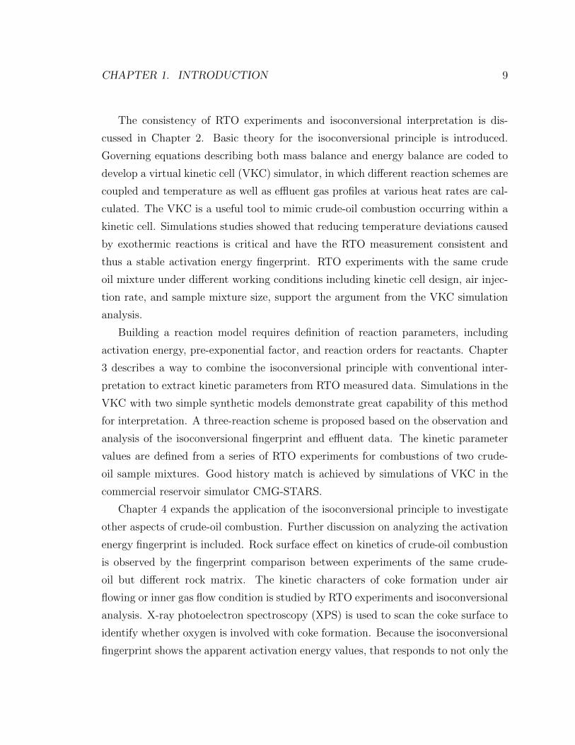
During an RTO experiment, the oxidation gas is preheated to the same tempera-
ture as that within the kinetic cell before injection. The gas reacts with the oil sample
for the period of residence time ∆t, and then the effluent gas flows out of the cell
chamber. This process is modeled as a CSTR process [43] [14]: 1. the fuel only exists
inside the reactor cavity because of the liquid phase or solid phase; 2. steady state is
considered for the gas reacting with fuel mixture so that the accumulation term for
gas species is zero.
Here are the governing equations describing the mass balances of liquid/solid phase
−dCf,idt
= rf,i, i = 1, 2, . . . , n (2.9)
and gas phase
0 =Fg,j,in − Fg,j,out
V+ rg,j, j = 1, 2, . . . ,m (2.10)
and the temperature variation
VdT
dt=Q̇−
∑mj=1 Fj,outCPj(T − Tj,in)∑n
i=1 CiCPi +∑m
j=1CjCPj+
∑ni=1 ∆HR,i(T )(riV )∑n
i=1CiCPi +∑m
j=1 CjCPj(2.11)
where rf,i and rg,j are net reaction rates for a liquid/solid phase and a gas phase
species respectively. Fg,j is molar flow rate of species j, V is the void volume of the
cell chamber, Q̇ is the heat flux from the furnace, CP is the heat capacity, and ∆HR
is the reaction enthalpy. The CSTR simulator is coded in MATLAB.
A synthetic scheme of four reactions is used in the simulator. The reactant fuel
is the original crude-oil and fuel∗ is the intermediate component. Reaction (a), (b)
and (d) are series reactions. Reaction (c) is the parallel reaction. For each reaction,
reaction orders for oxygen and fuel are unit. Arrhenius parameters are listed in Table
2.2.

CHAPTER 2. CONSISTENCY ISSUE 18
Table 2.2: Arrhenius parameters for the synthetic model
Reaction (a) (b) (c) (d)
Pre-exponential factor 1 2.93× 10⁵ 100 100L/(mole · s)Activation energy 63000 75000 125000 12000J/(mole · k)
fuel +O2k1−→ fuel∗ (a)
fuel∗k2−→ LTO +H2O (b)
fuel +O2k1−→ CO2 + CO +H2O (c)
LTO +O2k1−→ CO2 + CO +H2O (d)
Four-reaction synthetic reaction scheme.
Simulations of different heating rates are carried out. The O2 consumption and
the temperature histories are recorded. Both differential and integral isoconversional
methods are applied to process the data.
2.3 Consistency
2.3.1 RTO simulations
When applying the isoconversional principle to interpret apparent activation energy
from measurement data, the validation of this principle in a real kinetic experiment
needs to be investigated. This goes to the experimental consistency issue. Cinar
et al. [17] discussed some qualitative ideas to judge whether the measurements are
consistent or not . More analysis is needed to show how to work on kinetic experiments
correctly so that the measurements are consistent. This is significantly important to
make the measurement repeatable even with a different kinetic cell device [90]. In

CHAPTER 2. CONSISTENCY ISSUE 19
this subsection, simulations based on the synthetic model are discussed to show how
we should handle our experiments.
According to Eq. (2.6), the differential method has the basic principle for isocon-
versional method: at a certain extent of fraction conversion X,1/(RT ) and ln(dXdt
)
form a straight line and the slope of which is the apparent activation energy. Fried-
man performed experiments of the thermal degradation of plastic at different linear
heating rates. The isoconversional fingerprint interpreted from the TGA measure-
ment matched the documented result [35]. For crude-oil RTO experiments, because
of the intensive heat released from crude oil oxidation and the temperature control
strategy in which the furnace temperature is linearly prescribed, temperature within
the kinetic cell is very difficult to achieve a linear trend. Apparently, a rigorous test
of the consistency of experimental data for use in the isoconversional method has
never been discussed. The temperature deviation and its effect on the isoconversional
application are studied here as well. In the simulator where the temperature profiles
are calculated using the energy balance equation, the temperature deviation because
of the heat released is controlled by the values of reaction enthalpy. Linear temper-
ature histories are achieved by zero reaction enthalpies, and increasing the reaction
enthalpies increases the temperature deviations on the temperature histories.
Three cases are considered which are a linear temperature case (LT), a small
temperature deviation case (STD) and a large temperature deviation case (LTD).
The reaction enthalpies for each case are listed in Table 2.3. The LT case is an
ideal case without temperature deviation, and its activation energy fingerprint is well
interpreted by the isoconversional principle. The LTD case is an extreme case in
which a large amount of heat is released causing big temperature deviations of the
temperature profiles. In this study, the STD case is analyzed and the activation
energy result is compared with the LT and the LTD cases.
Figures 2.2 and 2.3 show the temperature and the oxygen consumption profiles at
different heat rates respectively. Two reaction stages, that are the low-temperature
oxidation and the high-temperature oxidation regions, are observed according to the
O2 consumption humps. Figure 2.4 shows temperature versus conversion X at each
heat rate. The curves of large heat rates are above those of low heat rates and there is

CHAPTER 2. CONSISTENCY ISSUE 20
Table 2.3: Heat of reaction values for different simulation cases
Reaction (a) Reaction (b) Reaction (c) Reaction (d)
LT 0 0 0 0STD -80000 40000 -100000 -100000LTD -100000 40000 -120000 -120000
no intersection between different curves. Figure 2.5 shows the consistency check plot,
in which the black solid lines represent the apparent activation energies according
to the isoconversional principle. The plot shows a linear trend of each line. Figure
2.6 shows the activation energy fingerprints obtained by the integral isoconversional
method. The STD fingerprint matches the LT fingerprint which is the ideal case, and
both of them represent the activation energy values listed in Table 2.2. For the LTD
case, the fingerprint represents the low temperature oxidation stage well, but there is
an oscillation at the high temperature oxidation stage. This oscillation is due to the
big temperature deviation caused by the large amount of heat released.
Based on the simulation results, a consistent measurement should follow: 1. when
plotting temperature versus conversion, larger heat rate curves should lie over lower
heat rate curves and there is no intersection between curves; 2. when plotting
ln(d[X]/dt) versus −1/(RT ), the connection for data points of different heat rates
at the same conversion should follow a linear trend and this trend is the activation
energy at that conversion X; 3. because of the much more complicated reaction ki-
netics for a real case of the crude oil combustion, big temperature deviations should
be avoided.
2.3.2 RTO experiments
Lab measurements of kinetic parameter are much more difficult because of the compli-
cated compositional character of crude-oil samples and the combustion mechanism.
Meanwhile, the noise introduced by temperature recording and from gas analyzer
data drift make it hard to obtain consistent measurement. Much effort is needed to
manage consistent measurements. According to the conclusion from simulations, a

CHAPTER 2. CONSISTENCY ISSUE 21
0 100 200 300 400 5000
200
400
600
800
1000
1200
1400
Time,min
Temperature, K
1.4 K/min
1.8 K/min
2.2 K/min
2.6 K/min
Figure 2.2: Temperature profiles for the small temperature deviation (STD) case. Foreach temperature profile, the first hump represents the low temperature oxidationstage and the second hump represents the high temperature oxidation stage.
0 100 200 300 400 5000
2
4
6
8
10
12
14
Time,min
O2 consumption, mole/m3
1.4 K/min1.8 K/min2.2 K/min2.6 K/min
Figure 2.3: O2 consumption profiles for the small temperature deviation (STD) case.For each O2 curve, the first hump represents the low temperature oxidation stageand the second hump represents the high temperature oxidation stage. The valleybetween the two stages is the transition zone.

CHAPTER 2. CONSISTENCY ISSUE 22
0 0.2 0.4 0.6 0.8 1400
500
600
700
800
900
1000
conversion
Temperature /K
1.4 K/min
1.8 K/min
2.2 K/min
2.6 K/min
Figure 2.4: Temperature versus conversion for the small temperature deviation (STD)case. The curve of large heat rate is over the one of low heat rate. There is nointersection between different curves.
−2.4 −2.2 −2 −1.8 −1.6 −1.4
x 10−4
−11.5
−11
−10.5
−10
−9.5
−9
−8.5
−1/(R*T)
ln(d
[x]/
dt)
1.4 K/min
1.8 K/min
2.2 K/min
2.6 K/min
Figure 2.5: A plot of ln(d[X]/dt) versus −1/(RT ) for consistency check. The blacksolid lines connect dots of the same conversionX of different heat rates. Trends of eachline are linear indication consistency. The slope represents the apparent activationenergy at that conversion X.

CHAPTER 2. CONSISTENCY ISSUE 23
0 0.2 0.4 0.6 0.8 15
6
7
8
9
10
11
12
13x 10
4
Conversion
Act
ivat
ion
Ene
rgy,
J/m
ole LT case
STD caseLTD case
Figure 2.6: Activation energy fingerprints interpreted from the linear temperature(LT) case, the small temperature deviation (STD) case and the large temperaturedeviation (LTD) case using the integral isoconversional method.
comparison study between two experiments are considered: a bad measurement with
large sample size and a good measurement with small sample size.
The crude oil sample used is an Alaskan crude oil with an API of 13.3. The sample
mixture composition is: 4 wt% of crude-oil; 80 wt% of 60 mesh fired sand; 8 wt% of
clay; 8 wt% of water. 100 psi back pressure is maintained within the kinetic cell.
The first measurement has 45 g of the sample mixture in KC1. The kinetic cell
back pressure is 100 psi. The air injection rate is 2 L/min. Five RTO experiments
are carried out. Temperatures within the cell chamber and the corresponding effluent
gas compositions are recorded. Figures 2.7 and 2.8 show the measurement results
for temperatures and O2 consumptions respectively. Two reaction stages, the low
temperature oxidation and the high temperature oxidation are observed. Figure 2.9
shows the temperature versus conversion curves. Some intersection parts are observed
between curves of different heat rate. In Figure 2.10 The relationship of 1/(RT ) and
ln(dXdt
) does not follow a linear trend in either the low temperature oxidation or
the high temperature oxidation region. Based on the analysis, the activation energy
fingerprint in Figure 2.11 is highly unstable and the values are not reliable. The plot

CHAPTER 2. CONSISTENCY ISSUE 24
0 50 100 150 200 250 300200
300
400
500
600
700
800
900
1000
Time,min
Tem
pera
ture
, K
3.00 K/min
2.78 K/min
2.53 K/min
2.30 K/min
2.26 K/min
Figure 2.7: Temperature histories for the RTO of Alaskan sample mixture: 13.3◦API, 45 grams of the sample mixture are used for each RTO experiment.
does not show characteristic LTO and HTO regions.
The second measurement is conducted using a smaller size of sample mixture of
25g in the KC1. The kinetic cell back pressure is 100 psi and the air injection rate
is 1.5 L/min. Temperatures within the cell chamber and the corresponding effluent
gas compositions are plotted in Figure 2.12 and Figure2.13, respectively. Figure
2.14 shows the temperature versus conversion curves. The curve of high heat rate is
over those of lower heat rates and there is no intersection of the curves. In Figure
2.15, the relationship of ln(dXdt
)and 1/(RT ) follow a linear trend in both the low
temperature oxidation and the high temperature oxidation stages. The consistency
analysis reveals good measurement for this case. The activation energy fingerprint in
Figure 2.16 exhibits two reaction stages and the activation energy values are reliable.
2.4 Repeatable RTO measurements
Three cases are conducted to test the repeatable character of RTO experiments for iso-
conversional interpretation. Based on the model-free character of the isoconversional
principle, the RTO measurements are conducted using the same sample mixture but
CHAPTER 2. CONSISTENCY ISSUE 25
0 50 100 150 200 250 3000
1
2
3
4
5
6
Time,min
O2 c
onsu
mpt
ion,
Mol
e fr
actio
n
3.00 K/min
2.78 K/min
2.53 K/min
2.30 K/min
2.26 K/min
Figure 2.8: O2 consumption histories for the RTO of Alaskan sample mixture: 13.3◦API, 45 grams of the sample mixture are used for each RTO experiment.
0 0.2 0.4 0.6 0.8 1400
450
500
550
600
650
700
750
800
850
900
conversion
Tem
pera
ture
/K
3.00 K/min
2.78 K/min
2.53 K/min
2.30 K/min
2.26 K/min
Figure 2.9: Temperature versus conversion for the RTO of Alaskan sample mixture:13.3 ◦API, 45 grams of the sample mixture are used for each RTO experiment.

CHAPTER 2. CONSISTENCY ISSUE 26
−2.3 −2.2 −2.1 −2 −1.9 −1.8 −1.7 −1.6
x 10−4
−10.5
−10
−9.5
−9
−8.5
−8
−7.5
−1/(R*T)
ln(d
[x]/d
t)
3.00 K/min
2.78 K/min
2.53 K/min
2.30 K/min
2.26 K/min
Figure 2.10: A plot of ln(d[X]/dt) versus −1/(RT ) for consistency check. The blacksolid lines connect dots of the same conversion X of different heat rates. Trends ofeach line are not linear for this measurement indicating inconsistent data. Alaskansample mixture: 13.3 ◦API, 45 grams of the sample mixture are used for each RTOexperiment.
0 0.2 0.4 0.6 0.8 10
1
2
3
4
5
6
7
8
9
10x 10
4
Conversion
Act
ivat
ion
Ene
rgy,
J/m
ole Friedman 1964
Vyazovkin 2001
Figure 2.11: Apparent activation energy fingerprint obtained from inconsistent datafor the RTO of Alaskan sample mixture: 13.3 ◦API, 45 grams of the sample mixtureare used for each RTO experiment.

CHAPTER 2. CONSISTENCY ISSUE 27
0 50 100 150 200 250 300 350 400200
300
400
500
600
700
800
900
Time,min
Tem
pera
ture
, K
2.64 K/min
1.93 K/min
1.74 K/min
1.54 K/min
Figure 2.12: Temperature histories for the RTO of Alaskan sample mixture: 13.3◦API, 25 grams of the sample mixture are used for each RTO experiment.
0 50 100 150 200 250 300 350 4000
0.1
0.2
0.3
0.4
0.5
0.6
0.7
0.8
0.9
Time,min
O2 c
onsu
mpt
ion,
Mol
e fr
actio
n
2.64 K/min1.93 K/min1.74 K/min1.54 K/min
Figure 2.13: O2 consumption histories for the RTO of Alaskan sample mixture: 13.3◦API, 25 grams of the sample mixture are used for each RTO experiment.

CHAPTER 2. CONSISTENCY ISSUE 28
0 0.2 0.4 0.6 0.8 1450
500
550
600
650
700
750
conversion
Tem
pera
ture
/K
2.64 K/min
1.93 K/min
1.74 K/min
1.54 K/min
Figure 2.14: Temperature versus conversion for the RTO of Alaskan sample mixture:13.3 ◦API, 25 grams of the sample mixture are used for each RTO experiment.
−2.5 −2.4 −2.3 −2.2 −2.1 −2 −1.9 −1.8 −1.7 −1.6
x 10−4
−10
−9.5
−9
−8.5
−8
−1/(R*T)
ln(d
[x]/d
t)
2.64 K/min
1.93 K/min
1.74 K/min
1.54 K/min
Figure 2.15: A plot of ln(d[X]/dt) versus −1/(RT ) for consistency check. The blacksolid lines connect dots of the same conversion X of different heat rates. Trends ofeach line are linear for this measurement. Alaskan sample mixture: 13.3 ◦API, 25grams of the sample mixture are used for each RTO experiment.

CHAPTER 2. CONSISTENCY ISSUE 29
0 0.2 0.4 0.6 0.8 10
0.2
0.4
0.6
0.8
1
1.2
1.4
1.6
1.8
2x 10
5
Conversion
Act
ivat
ion
Ene
rgy,
J/m
ole
Friedman 1964Vyazovkin 2001
Figure 2.16: Apparent activation energy fingerprint obtained from consistent data forthe RTO of Alaskan sample mixture: 13.3 ◦API, 25 grams of the sample mixtureare used for each RTO experiment.
under different working conditions, including different kinetic cell designs, different
sample mixture sizes and different air injection rates.
The sample mixture used is the Alaskan crude-oil - 2.2 wt%; 60 mesh fired sand
- 88.9 wt%; clay - 0 wt% and water - 8.9 wt%. A 100 psi back-pressure is applied for
all experiments. The first case uses KC1. 18 g of the sample mixture is put into the
kinetic cell and 1 L/min gas injection rate is used. The second case uses KC2. 25 g
of the sample mixture is used and 1.5 L/min gas injection rate is applied. The third
case uses KC3. 10 g of the sample mixture is used and 1 L/min gas injection rate is
applied. For each case, RTO experiments of different heat rates are conducted.
The activation energy fingerprints of the three cases are plotted in Figure 2.17.
The integral isoconversional method is applied. These curves demonstrate very close
values of activation energy as a function of conversion. They reveal the model-free
character of the isoconversional principle and the repeatability of RTO experiments
for crude-oil combustion kinetic studies.
It is well known that the clay within the matrix favors the ISC process by adding
interfacial area and a catalytic affect from the heavy metal derivatives [25][111]. The

CHAPTER 2. CONSISTENCY ISSUE 30
0 0.2 0.4 0.6 0.8 10
0.5
1
1.5
2
2.5
3x 10
5
Conversion
Act
ivat
ion
Ene
rgy,
J/m
ole Case 1
Case 2Case 3
Figure 2.17: Activation energy fingerprints for three cases with different sample massof identical composition. Case 1: KC1 is used, 18 grams of the mixture is used andair injection rate is 1 L/min; Case 2: KC2 is used, 25 grams of the mixture is usedand air injection rate is 1.5 L/min; Case 3: KC3 is used, 10 grams, of the mixtureis used and air injection rate is 1 L/min
clay within a sample mixture changes the reaction mechanism and reduces the appar-
ent activation energies. This result is easily observed when we compare the activation
energy fingerprints for the Alaskan crude-oil cases with and without clay in Figure
2.16 and Figure 2.17 respectively. More details on the rock surface effect and kinetic
information in the activation energy fingerprint are discussed in Chapter 4.
2.5 Conclusion
The isoconversional principle is successfully applied to interpret apparent activa-
tion energy for crude-oil combustion within a continuous flow stirred tank reactor.
Ramped temperature oxidation experiments are conducted in the kinetic cell platform
in which temperatures as well as production gas data are recorded. A simulator is de-
veloped for describing the combustion process within the kinetic cell. The simulation
with a synthetic reaction model and RTO experiments with Alaskan crude-oil mixture
show how to manage successful RTO experiments: because of the exothermic reaction

CHAPTER 2. CONSISTENCY ISSUE 31
mechanism of crude-oil, reducing the amount of heat generated by the reaction is nec-
essary to keep measurements reliable and consistent. Three sets of RTO experiments
of different reactor designs, different air injection rates and different sample mixture
sizes support that the model-free character of the isoconversional principle and its
promising feature to unlock the complicated kinetics of the ISC process.

Chapter 3
Isoconversional modeling and
simulation
When performing in-situ combustion simulations, a reaction kinetic model is needed
to couple with other physical models, such as fluid flow through porous media and
thermodynamic behavior including phase changes. Kinetic studies of crude-oil com-
bustion offer parameters for reaction rate modeling. According to Eq.2.4, these pa-
rameters include activation energy E, pre-exponential factor A, and reaction orders
a and b for oxygen partial pressure and fuel concentration, respectively. A reliable
kinetic model should capture as many critical characters of the ISC process as possi-
ble, whereas the reaction scheme should consist of as few components and reactions
as necessary to reduce the cost of numerical computations.
Kinetics research of crude oil combustion in porous media is complicated by sev-
eral factors. The first is the multi-component character of a crude-oil. Normally, the
crude oil sample consists of hundreds of identified light and heavy hydrocarbon com-
ponents that dissolve into each other. The simplest hydrocarbon component, CH4,
needs about 37 species and 351 irreversible reactions as its comprehensive chemi-
cal mechanism to account for its oxidation performance [51]. When analysis goes
to a heavy component, the detailed reaction kinetic model is impractically complex.
Meanwhile analyzing the crude oil by separating components or fractions dismisses
32

CHAPTER 3. ISOCONVERSIONAL MODELING AND SIMULATION 33
the interaction between components. This is considered to be an important factor al-
tering the reaction paths. Secondly, the crude oil is mixed with rock matrix. The rock
mineralogy, such as carbonates, surface area, and metallic catalyst has non-negligible
influence on the reaction paths, thus, the apparent behavior of the combustion. The
third factor is the multiphase behavior of the crude oil. The reaction kinetic per-
formance of a certain species may be different in different phases, such as gas phase
and liquid phase [79]. When accounting for phase behavior across a wide tempera-
ture range from ambient to the peak combustion temperature such as 600 ◦C, the
thermodynamic equilibrium changes intensively. Therefore the effect of phase be-
havior on the combustion is nontrivial. The last but not least is the wide range of
temperatures associated with heat conduction as well as heat released from exother-
mic reactions. Very limited experimental tools can describe the kinetic behavior in
such a complicated condition. Conventionally, isothermal experiments were carried
out. This technique needs to keep temperature constant at several values that artifi-
cially narrows the temperature range. The measured data do not represent the entire
combustion behavior of the crude oil in the ISC process [113]. As a result, ramped
temperature oxidation (RTO) within a kinetic cell was developed [31][32]. In RTO,
the experiments are conducted non-isothermally. Temperature within a kinetic cell is
increased by an external heat source, from ambient to a very high termination tem-
perature. Effluent gas data are recorded by a gas analyzer. Interpretation methods
include those applied to the isothermal experiments and the isoconversional principle.
It is believed that the isoconversional principle has more advantages than the con-
ventional methods with respect to its model-free nature and robustness in conducting
reliable measurement [16][17].
As discussed in Chapter 2, activation energy E of crude oil combustion within a
kinetic cell is dynamically changed and the apparent values are presented against the
conversion X in the isoconversional fingerprint. Other kinetic parameters, like the
pre-exponential factor and reaction orders for oxygen partial pressure and fuel concen-
tration, are still unknown. This chapter introduces an approach combining both the
isoconversional principle and the conventional interpretation method to define reac-
tion parameters for the combustion model. The approach is applied in two synthetic

CHAPTER 3. ISOCONVERSIONAL MODELING AND SIMULATION 34
cases with the same reaction scheme, but different reaction model. A three-reaction
scheme is proposed for the combustion of two different crude-oil sample mixtures and
the reaction parameters are interpreted by the proposed method.
3.1 Defining kinetic parameters
According to the literature review, the isoconversional principle is widely applied to
interpret activation energies for solid decomposition processes [114]. Mass variation
is measured as a function of time and the corresponding ramped temperatures are
recorded. The conversion is defined as the accumulated mass change divided by
the original mass. Theoretical analysis and experimental measurement show the
isoconversional principle works well on solid component reactions [114].
When this principle is applied to study ISC reaction kinetics by a continuous
flow reactor, the effluent gas rather than the mass of the fuel inside the reactor
chamber is measured. Application of the principle to interpret kinetic parameters
is an issue. Meanwhile, other kinetic parameters, such as pre-exponential factor
and reaction orders, are still unknown. Cinar et al. described governing equations
derived for the kinetic cell system and the definition of conversion in terms of oxygen
consumption [14][15][16], but the connection between the conventional method and
the isoconversional method is not clear. Understanding the connection between the
conventional method and the isoconversional method, as well as different time scales
in the process of the flow reactor system is necessary. Discussion on the connection
also provides some prerequisites to run successful RTO experiments for isoconversional
interpretation.
In order to find out the connection between the conventional method and the
isoconversional method, two different time scales in the flow reactor system need to
be introduced. One time scale is the entire reaction period. At this time scale, we
record temperatures and production gas compositions at a certain frequency (usually
per second). A typical RTO measurement is shown in Figure 3.1, including histories
for temperatures, oxygen consumption and carbon oxides fractions in the effluent
gas stream. We process these measurements by the isoconversional principle to get

CHAPTER 3. ISOCONVERSIONAL MODELING AND SIMULATION 35
Figure 3.1: Ramped temperature oxidation measurement data
kinetic parameters.
The conversion factor in terms of oxygen consumption up to a time t is defined as
X =
∫ t0
∆xO2(t)dt∫∞0
∆xO2(t)dt(3.1)
Where X is the oxygen conversion factor, and ∆xO2 is oxygen consumed as a function
of time:
∆xO2 = x◦O2− x′O2
(3.2)
where x′O2is the oxygen molar fraction in the outlet stream and x◦O2
is the oxygen
molar fraction in the inlet stream.
The isoconversional method is a model-free process to interpret activation en-
ergy. Little manipulation of measurement data is needed for processing. So it is very
convenient, and it has many advantages as compared to the conventional method of
obtaining activation energy values. It is not that straightforward to obtain the for-
mula of a reaction model in terms of oxygen conversion X. Some research describes

CHAPTER 3. ISOCONVERSIONAL MODELING AND SIMULATION 36
how to interpret the pre-exponential factor using the isoconversional principle. A
reaction model of a certain reaction order is presumed. One example is polymer
degradation modeling. The overall degradation rate is conventionally expressed by
nth order model of sample mass [37]. In an RTO measurement where effluent gas
compositions are recorded, however, the fuel mass within the kinetic cell is not mea-
sured. Furthermore, it is very difficult to describe the fuel concentration using the
oxygen conversion X because of the multi-step reaction scheme and the unknown
stoichiometry.
On the other hand, conventional expression of reaction rates describes a reaction
model in terms of reactant concentrations as
−dCfdt
= A∗exp(− E
RT)Ca
O2Cbf (3.3)
When a reactant is in the gas phase, such as oxygen, partial pressure of the gas is
used in place of the concentration:
−dCO2
dt= Aexp(− E
RT)P a
O2Cbf (3.4)
In the RTO experiment, oxygen concentration is approximated as
CO2 =
xO2PtotalV
T0
V=xO2Ptotal
T0
(3.5)
In terms of molar fraction of oxygen, xO2 , Eq. 3.4 is written as
−dxO2
dt= (AT0P
a−1total)exp(−
E
RT)xaO2
Cbf (3.6)
To apply Eq. 3.6 to interpret kinetic parameters from measured RTO data, the
other time scale related to the gas volumetric flow rate is introduced. The process
of the continuous flow reactor is simplified in Figure 3.2. The residence time ∆t is
defined in Eq. 3.7. If ∆t is small enough, T is considered to be the same at the inlet
and the outlet streams. This condition is achieved by a relatively high gas injection
rate and increasing temperature slowly in a RTO experiment. The injection gas is

CHAPTER 3. ISOCONVERSIONAL MODELING AND SIMULATION 37
Figure 3.2: Continuous flow reaction process during RTO
preheated to the kinetic cell temperature in the inlet portion of the furnace. So Eq.
3.6 is written as
∆t =Void volume inside the kinetic cell
Volumetric flow rate(3.7)
∆xO2
∆t= (AT0P
a−1total)exp(−
E
RT)(x◦O2
)aCbf (3.8)
For a normal RTO experiment, where the gas injection rate is 1.5 L/min or above
and the temperature heat rate is 3 K/min or lower, the condition is fulfilled. Together
with Eq. 2.5 and Eq. 3.8, we can estimate activation energy E, pre-exponential factor
A, and reaction order a and b.
3.1.1 Defining activation energy
By applying the isoconversional principle that considers the reaction model to be
only a function of conversion X and independent from temperature T , we obtain the
activation energy E by post processing RTO measured data. Taking the logarithm
on both sides of Eq. 2.5, we have

CHAPTER 3. ISOCONVERSIONAL MODELING AND SIMULATION 38
ln(dX
dt) = ln(Af(X))− E
RT(3.9)
By plotting ln(dXdt
) vs. − 1RT
of RTO experiments, activation energy values as a
function of the conversion factor X are interpreted. This is the differential form of the
isoconversional principle. Other adjusted forms including the integral formulations
are developed [112][115], but the differential form is fundamental and it provides us
direct clues on handling RTO experiments correctly as discussed in Chapter 2.
3.1.2 Defining reaction orders
When the activation energy values are interpreted, the fuel reaction order is solved.
Defining α as the oxygen conversion within a reaction stage, and according to the
isoconversional principle, fuel conversion is proportional to oxygen conversion,
Cbf,X = ((1−X)C◦f )b (3.10)
where C◦f is the initial fuel concentration. Considering Eq. 3.8 for one of the RTO
measurements at two different conversions, X1 and X2 in a certain reaction stage
∆xO2,X1
∆t= (AT0P
a−1total)exp(−
E
RTX1
)(x◦O2)aCb
f,X1(3.11)
∆xO2,X2
∆t= (AT0P
a−1total)exp(−
E
RTX2
)(x◦O2)aCb
f,X2(3.12)
substituting Cbf,α1 and Cb
f,α2 into Eq. 3.10 and combining Eq. 3.11 and Eq. 3.12
together, one can get
∆xO2,X1
∆xO2,X2
= exp(E
RTX2
− E
RTX1
)(1−X1
1−X2
)b (3.13)
Solving Eq. 3.13 provides the value for fuel reaction order, b.
According to Eq. 2.5 and Eq. 3.8, if the reaction mechanism is well defined, it
should be independent of partial pressure of oxygen. In the following section, RTO
experiments of different injected oxygen fractions support this argument. Considering
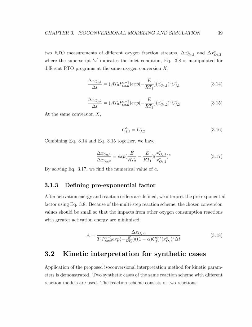
CHAPTER 3. ISOCONVERSIONAL MODELING AND SIMULATION 39
two RTO measurements of different oxygen fraction streams, ∆x◦O2,1and ∆x◦O2,2
,
where the superscript ′◦′ indicates the inlet condition, Eq. 3.8 is manipulated for
different RTO programs at the same oxygen conversion X:
∆xO2,1
∆t= (AT0P
a−1total)exp(−
E
RT1
)(x◦O2,1)aCb
f,1 (3.14)
∆xO2,2
∆t= (AT0P
a−1total)exp(−
E
RT2
)(x◦O2,2)aCb
f,2 (3.15)
At the same conversion X,
Cbf,1 = Cb
f,2 (3.16)
Combining Eq. 3.14 and Eq. 3.15 together, we have
∆xO2,1
∆xO2,2
= exp(E
RT2
− E
RT1
)(x◦O2,1
x◦O2,2
)a (3.17)
By solving Eq. 3.17, we find the numerical value of a.
3.1.3 Defining pre-exponential factor
After activation energy and reaction orders are defined, we interpret the pre-exponential
factor using Eq. 3.8. Because of the multi-step reaction scheme, the chosen conversion
values should be small so that the impacts from other oxygen consumption reactions
with greater activation energy are minimized.
A =∆xO2,α
T0Pa−1totalexp(− E
RTα)((1− α)C◦f )b(x◦O2
)a∆t(3.18)
3.2 Kinetic interpretation for synthetic cases
Application of the proposed isoconversional interpretation method for kinetic param-
eters is demonstrated. Two synthetic cases of the same reaction scheme with different
reaction models are used. The reaction scheme consists of two reactions:

CHAPTER 3. ISOCONVERSIONAL MODELING AND SIMULATION 40
fuel +O2k1−→ fuel∗ (syn.1)
fuel∗ +O2k2−→ CO + CO2 +H2O (syn.2)
In the reaction scheme, fuel and fuel∗ are in the liquid phase and other species
are in the gas phase. The virtual kinetic cell simulator uses reactant concentration
to calculate the oxygen uptake rates (partial pressure expression and concentration
expression for the rate equation are consistent). Eq. 3.18 is rewritten as
A =∆CO2,α
exp(− ERTα
)((1− α)Cf,initial)b(C◦O2)a∆t
(3.20)
Other input parameters used in VKC are listed below:
• Pressure: Ptotal = 100 psi;
• Void volume within the kinetic cell chamber: V = 40 cm3;
• Volumetric flow rate: V̇ = 2 L/min;
• Fuel initial concentration in the cell: C◦f = 20000 mole/m3;
• Oxygen initial concentration in the gas stream: C◦O2= 222.49 mole/m3;
• Oxygen molar fraction in the inlet stream: 80% or 100%.
3.2.1 Synthetic case of unit reaction orders
The first synthetic case considers unit reaction orders for both fuel and oxygen. The
kinetic parameters are listed in Table 3.1.
The simulation results of temperature and oxygen consumption as a function of
conversion are shown in Figure 3.3 for the 80% oxygen case and Figure 3.4 for 100%
oxygen case. Figure 3.5 shows the activation energy fingerprints for both cases. The
80% oxygen case and 100% oxygen case reveal similiar behavior on the isoconversional
fingerprint. Oxygen partial pressure does not alter the reaction paths.

CHAPTER 3. ISOCONVERSIONAL MODELING AND SIMULATION 41
Table 3.1: Arrhenius parameters used in the synthetic case of unit reaction orders
A, 1/(mole · s) E, J/mole Heat of reaction, J/mole a b
Reaction syn.1 1 63000 -40000 1 1Reaction syn.2 100 120000 -60000 1 1
Calculation is done based on one of the RTO experiments in Figure 3.3 and Eq.
3.13 to define the fuel’s reaction order b. From Figure 3.5(a), the activation energy
for the reaction syn.1 and syn.2 are 63000 J/mole and 120000 J/mole respectively.
From Figure 3.3(b) and 3.3(a), we pick up the conversion values of 0.1 and 0.2 for the
reaction syn.1 and 0.6 and 0.7 for the reaction syn.2. The reaction syn.1 consumes
about 50% of the total oxygen, and the reaction syn.2 consumes about the rest 50%
of the total oxygen. So for the reaction syn.1, we can get b = 1.0136. We do the same
calculation for the reaction syn.2, and we can get b = 0.9976.
In order to get the reaction order a for oxygen, oxygen fraction within the inlet
stream needs to be changed. The 100% oxygen case is considered and the calculation
is based on Eq. 3.17. We pick up the conversion values of 0.2 for the reaction syn.1
and 0.7 for the reaction syn.2. So ∆xO2,1 = 5.57 and ∆xO2,2 = 5.76. The parameter
a is calculated by Eq. 3.17 and is 0.9924 for the reaction syn.1. The same calcualtion
is done for reaction syn.2, and a = 0.9918.
Once the reaction orders are interpreted, according to Eq. 3.20, the pre-exponential
factor A is calculated. The 80% oxygen case is used to interpret A. For the reaction
syn.1, The residence time is ∆t = 1.2 sec based on Eq. 3.7. So A = 0.9890 1/(mole·s)for reaction syn.1 and A = 101.7582 1/(mole · s) for reaction syn.2.
The error analysis between the interpreted kinetic parameters and the values of
pre-assumed model are compared in Table 3.2. The comparison shows acceptable
matches.
3.2.2 Synthetic case of non-unit reaction orders
The second synthetic case uses non-unit reaction orders. The kinetic parameters are
listed in Table 3.3. When the reaction orders are greater than one, they favor the

CHAPTER 3. ISOCONVERSIONAL MODELING AND SIMULATION 42
(a) Temperature vs. conversion
(b) O2 consumption vs. conversion
Figure 3.3: Simulation results for the synthetic case of unit reaction orders: 80%oxygen in the injection gas stream.

CHAPTER 3. ISOCONVERSIONAL MODELING AND SIMULATION 43
(a) Temperature vs. conversion
(b) O2 consumption vs. conversion
Figure 3.4: Simulation results for the synthetic case of unit reaction orders: 100%oxygen in the injection gas stream.

CHAPTER 3. ISOCONVERSIONAL MODELING AND SIMULATION 44
(a) Activation energy fingerprint for the O2 = 80% case
(b) Activation energy fingerprint for the O2 = 100% case
Figure 3.5: Activation energy fingerprints for unit reaction order cases of differentoxygen compositions in the injection stream: both cases reveal similar fingerprintsbecause of the identical reaction scheme.

CHAPTER 3. ISOCONVERSIONAL MODELING AND SIMULATION 45
Table 3.2: Error analysis for the synthetic case of unit reaction orders
A, 1/mole*s E, J/mole a b
Reaction 4.2a 1 63000 1 1Estimation value 0.9890 63000 0.9924 1.0136Rel Error 0.011 0 0.0076 0.0136Reaction 4.2b 100 120000 1 1Estimation value 101.7582 120000 0.9918 0.9976Rel Error 0.0176 0 0.0082 0.0024
Table 3.3: Arrhenius parameters used in the synthetic case of non-unit reaction orders
A, 1/mole*s E, J/mole Heat of reaction, J/mole a b
Reaction 4.2a 1 63000 -20000 2 1Reaction 4.2b 100 120000 -40000 1.5 1
reaction rates and thus the heat released, so the heat of reaction is reduced. Other
parameters are the same as the synthetic case of unit reaction orders.
For the case of 80% oxygen, the simulation results are shown in Figure 3.6, and
for the case of 100% oxygen, the simulation results are shown in Figure 3.7. The
same calculation procedure as the synthetic case of unit reaction orders is used, and
the interpreted results and error analysis are listed in Table 3.4.
Table 3.4: Error analysis for the non-unit reaction order case
A, 1/(mole · s) E, J/mole a b
Reaction 4.2a 1 63000 2 1Estimation value 0.9839 63000 1.9864 0.9939Rel Error 0.0161 0 0.0068 0.0061Reaction 4.2b 100 120000 1.5 1Estimation value 100.6609 120000 1.5148 1.0073Rel Error 0.0066 0 0.0099 0.0073

CHAPTER 3. ISOCONVERSIONAL MODELING AND SIMULATION 46
(a) Temperature vs. conversion
(b) O2 consumption vs. conversion
Figure 3.6: Simulation results for the synthetic case of non-unit reaction orders: 80%oxygen in the injection gas stream.
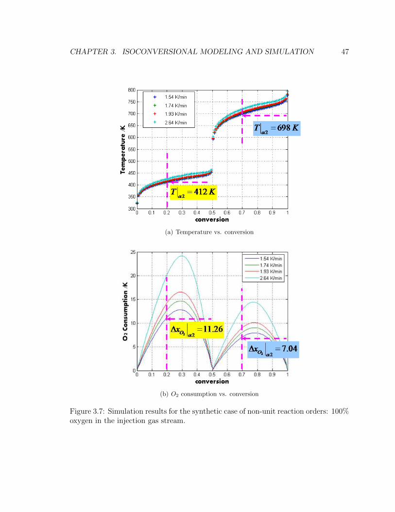
CHAPTER 3. ISOCONVERSIONAL MODELING AND SIMULATION 47
(a) Temperature vs. conversion
(b) O2 consumption vs. conversion
Figure 3.7: Simulation results for the synthetic case of non-unit reaction orders: 100%oxygen in the injection gas stream.

CHAPTER 3. ISOCONVERSIONAL MODELING AND SIMULATION 48
(a) Activation energy fingerprint for the O2 = 80% case
(b) Activation energy fingerprint for the O2 = 100% case
Figure 3.8: Activation energy fingerprints for non-unit reaction order cases of differentoxygen compositions in the injection stream: both cases reveal similar fingerprintsbecause of the identical reaction scheme.

CHAPTER 3. ISOCONVERSIONAL MODELING AND SIMULATION 49
3.2.3 Discussion
The interpretation procedure applied in the synthetic cases shows acceptable results
of the interpreted parameters. Reaction order for fuel is interpreted from a set of RTO
experiments under the same oxygen composition injection condition, while reaction
order for oxygen concentration or oxygen partial pressure is interpreted from a series
of RTO experiments under different oxygen composition in the gas stream. The
interpretation procedure is carried out for the real cases to build kinetic reaction
models for crude-oil combustion.
3.3 Kinetic interpretation and simulation
3.3.1 Gridding strategy
To verify the different reaction kinetic models proposed, simulations of the combustion
process within the kinetic cell are carried out using CMG-STARS [19]. A radial
gridding strategy of 4×1×7 is applied to divide the RTO system into five functional
zones: the crude-oil sample mixture is located in the center of the kinetic cell chamber;
two sand dispersion zones are at the bottom and on the top part of the cell cavity;
outside of the cell chamber is the stainless steel tube body of the kinetic cell, air
zones are in between the cell body and the furnace, and the outermost zone is the
electric furnace. The dimensions of each zone are the same as the real kinetic cell
system in the lab. Figure 3.9 demonstrates the gridding strategy as described. The
electric furnace is simulated by the outermost grid blocks with a large value of the
heat capacity. Heat flux is added to the grid block and a linear temperature profile
is imposed. The large value of the heat capacity reduces the influence of interior grid
blocks. The injection well is located at the bottom cap of the the kinetic cell, that is
heated up during a RTO process so that the injected gas is preheated. Then, the gas
stream travels through the sand at the inlet of the cell chamber. During this period,
the gas temperature is increased even more. The preheating process in simulation is
very close to the real preheating stage in an RTO experiment. While the gas keeps
going upward, it contacts with the sample mixture at the center of the cell chamber

CHAPTER 3. ISOCONVERSIONAL MODELING AND SIMULATION 50
and then reactions take place with temperature increasing. The production well is
located at the cap on top of the kinetic cell and the production gas is conducted
through the production well to the gas analyzer.
3.3.2 Kinetic reaction scheme
There are a number of proposed reaction schemes that capture the combustion behav-
ior during an ISC process under different conditions [6][30][17]. Based on the work
of Hayashitani et al. [48] and Adegbesan et al. [2], Belgrave et. al. [6] proposed
a pseudo-mechanistic reaction scheme for modeling the ISC of Athabasca bitumen.
The reaction scheme divides the crude oil composition into fractions of maltenes and
asphaltenes. Three reactions are used for thermal cracking, two reactions for the
low temperature oxidation stage and one reaction for the high temperature oxidation
stage:
Maltenek1−→ Asphaltenes (Thermal cracking)
Asphaltenesk2−→ Coke (Thermal cracking)
Asphaltenesk3−→ Gas (Thermal cracking)
Maltene+O2k4−→ Asphaltenes (LTO)
Asphaltenes+O2k5−→ Coke (LTO)
Coke+O2k6−→ CO2 + CO +H2O (HTO)
Reaction scheme proposed by Belgrave et al. [6].
By processing RTO experiments and observing identified reaction stages from
effluent data, Dechelette et. al. [23] proposed a three-reaction scheme to capture the
two distinct combustion stages. They use two kinds of coke components to mimic the
HTO performance:

CHAPTER 3. ISOCONVERSIONAL MODELING AND SIMULATION 51
Figure 3.9: Radial griding strategy (4 × 1 × 7 for r × θ × h) to mimic the kineticcell system in CMG-STARTS (the kinetic cell/furnace schematic diagram is adaptedfrom a figure in Cinar’s thesis [17].

CHAPTER 3. ISOCONVERSIONAL MODELING AND SIMULATION 52
Oil +O2k1−→ Coke1 (LTO)
Coke1 +O2k2−→ Coke2 + CO + CO2 +H2O (HTO)
Coke2k3−→ CO + CO2 +H2O (HTO)
Reaction scheme proposed by Dechelette et al. [23].
Cinar et al. [17] were the first to apply the isoconversional principle together
with RTO experiments to build a reaction model for ISC. The result is based on the
observation of the effluent gas data from RTO experiments and the isoconversional
fingerprint of activation energies. At least two different coke formation reactions are
necessary for conditions of under nitrogen and under air, and there should be two
distinct coke species for LTO and HTO respectively. Stoichiometry of the proposed
reaction scheme for a certain crude-oil/sand mixture is interpreted from effluent gas
data. The isoconversional activation energy fingerprint is used to identify reaction
stages and give initial activation energy values to each reaction. Reaction orders are
all assumed to be unity, and activation energies, pre-exponential factors are tuned
by an optimization strategy. After the optimization process, the kinetic cell simula-
tions showed good matches on both temperature and effluent gas histories with RTO
measurements, however, the activation energy values are different from those on the
isoconversional fingerprint.
Oilk1−→ Coke2 + volatiles (Ignition)
Oilk2−→ volatiles (Ignition)
Oil +O2k3−→ Coke1 +H2O (LTO)
Coke1 +O2k4−→ +CO + CO2 +H2O (LTO)
Coke1k5−→ Coke2 (MTO)
Coke2k6−→ CO + CO2 +H2O (HTO)
Reaction scheme proposed by Cinar et al.[17].

CHAPTER 3. ISOCONVERSIONAL MODELING AND SIMULATION 53
Based on the review of proposed reaction models in publication, a reaction model
for ISC combustion, whether it is complicated or simple, needs to capture at least
two identified reaction stages during the ISC process: low temperature oxidation and
high temperature oxidation. A complicated reaction model captures more details,
because there are more parameter variables which means more degrees of freedom.
The complicated model however is expensive to couple into a reservoir simulator
and has more parameters to define and most of which are difficult to interpret from
experimental measurement. Therefore, tuning the parameter by an optimization
routine or manually persists in ISC simulations. This tuning process at some level
overshadows the physical meaning of the reaction model by a mathematical solution.
On the other hand, reaction orders for reactants are normally presumed as unit. Thus,
the compensation of degree of freedom comes from adding more reactions.
Therefore, proposing a simple reaction scheme and defining its parameters to
the greatest extent possible from lab measurement is more preferred. Based on
observation of effluent gas data together with isoconversional fingerprint, a three-
reaction model is proposed for the combustion of two different crude-oil/sand mix-
tures, Alaskan crude oil mixed with fired sand of 60 mesh and clay and Karamay
crude oil mixed with reservoir sand. The proposed reaction Scheme 3.24 describes
the three major reaction stages: ignition, LTO and HTO. The ignition reaction does
not change the oil property, it plays like a threshold to retard reactions happening at
low temperature.
Oilk1−→ Oil∗ (Ignition)
Oil∗ +O2k2−→ Coke+ CO2 + CO +H2O + V olatiles (LTO)
Coke+O2k3−→ CO2 + CO +H2O (HTO)
Reaction scheme 3.24
RTO experiments are carried out to define the stoichiometry of the reaction scheme
and interpret kinetic parameters for the rate law model. As described previously,
at least two RTO experiments at different heat rates are needed to interpret the

CHAPTER 3. ISOCONVERSIONAL MODELING AND SIMULATION 54
reaction order of fuel, and two RTO experiments of different oxygen composition
in the injection stream are needed to interpret the reaction order of oxygen partial
pressure. For each crude oil mixture of Alaska crude oil or Karamay crude oil, four
sets of RTO experiments under four different oxygen composition injection are carried
out. This is also used to check that the reaction paths are consistent under different
oxygen composition.
3.3.3 Alaskan oil sample
The Alaskan crude-oil (13.3 ◦API) sample mixture of 25 grams is used in each of the
RTO experiments. The mixture composition is 2.04 wt% crude-oil, 8.16 wt% water,
81.63 wt% fired sand of 60 mesh and 8.16 wt% clay. Based on the crude-oil fraction
of the mixture, 0.51 grams of crude-oil are initially inside the kinetic cell. The air
injection rate is 1.5 L/min at the standard condition (25 ◦C and 1.01325× 10⁵ Pa).
The RTO experiment with the heat rate of 1.85 K/min is selected for stoichiometry
calculation (Figure 3.10).
The first step is defining the stoichiometry for the HTO reaction in Scheme 3.24.
From Figure 3.10, CO2/CO is 3.8, O2/CO2 is 1.18. Using mass balance, H2O/CO2
is 0.105 and H/C is 0.166. With this information, the chemical formula for coke is
CH0.166, and the stoichiometry for the HTO reaction is calculated by the balance of
elements.
The entire reaction period of the RTO experiment is 18600 seconds. Processing
the integral of the production gas of both CO and CO2 over the reaction period, an
amount of 1.66×10⁻² mole of carbon C is captured by the gas analyzer in the form of
carbon oxides. Considering that oxygen consumption contributes to the production
of carbon oxides and water, the apparent hydrogen content within the crude-oil is
calculated by subtracting oxygen in carbon oxides, and it is 2.99× 10⁻² mole. Thus,
a total mass of carbon and hydrogen from crude-oil that is involved in reactions
recorded by gas analyzer is 0.23 gram. The mass difference between the initial crude-
oil and total mass of carbon and hydrogen recorded by the gas analyzer is caused by
volatile components of the crude oil or other produced hydrocarbon gas that can’t

CHAPTER 3. ISOCONVERSIONAL MODELING AND SIMULATION 55
be recognized by the gas analyzer. Both of the volatile components are hydrocarbon
gases are grouped into V C in the reaction scheme. Based on mass balance, 44.86%
of the original crude oil reacts with oxygen and generates coke, carbon oxides and
water, and the other 55.14% is grouped into V C. From Figure 3.10, in the LTO stage,
the ratio of CO2 and CO is 2.42, and O2/CO2 is around 3. The crude oil molecular
weight is estimated by adjusting its value to match the peak oxygen consumption of
either LTO or HTO, and it is 615 g/mole. The molar ratio of O2 and the coke is
estimated by the peak oxygen consumption ratio of LTO and HTO. H2O can not be
estimated from the measurement, so it is used to balance the mass of products for
the LTO reaction. The proposed reaction scheme for Alaska crude-oil mixture is:
Oilk1−→ Oil∗ (Ignition)
Oil∗ + 15O2k2−→ 12.5CH0.166 + 5CO2 + 2.07CO + 18.11H2O + 12.11V C (LTO)
CH0.166 + 0.9O2k3−→ 0.79CO2 + 0.21CO + 0.08H2O (HTO)
Reaction scheme 3.25
After defining the stoichiometry, kinetic paramters for each of the reactions are
interpreted. Four sets of RTO experiments using different oxygen composition in the
injection gas are carried out. The four activation energy fingerprints are plotted in
Figure 3.11. The 35% oxygen case does not reveal a consistent fingerprint as those
with oxygen compositions of 16% to 21%. So this case is not taken into consideration
for parameter interpretation. The ignition reaction take places at the very begining.
From Figure 3.11, the activation energy value for the ignition reaction is about 1.0×10⁵ J/mole. The pre-exponential factor can be estimated from the starting point
of oxygen consumption and A is 1.0 × 10¹⁰ 1/(mole · min). For the LTO reaction,
the activation energy is about 8.5 × 10⁴ J/mole. Two conversion X values, 0.2 and
0.22, are chosen to process the calculation for the fuel reaciton order. The RTO
experiments used are the one with air injection. The LTO reaction begins at about
X = 0 and ends at around X = 0.6. Based on Eq. 3.13, the LTO reaction order
for fuel is b = 1.83. Calculating the oxygen partial pressure reaction order, the

CHAPTER 3. ISOCONVERSIONAL MODELING AND SIMULATION 56
conversion value of 0.2 is used for RTO experiments of different oxygen compositon
in the injection gas. Based on Eq. 3.17, the reaction order for oxygen is a = 0.9. The
residence time is calcuated under the 100 psi condition and it is 0.056 min. The intial
fuel concentration is about 6.87 × 10⁻⁵ mole/cm3. Based on Eq. 3.18, A is about
3.69 × 10¹⁵ 1/(mole · min). The same interpretation for HTO reaction parameters
is conducted. The HTO activation energy is interpreted from Figure 3.11 and it is
around 1.3 × 10⁵ J/mole. Two conversion X values, 0.7 and 0.75, are chosen to
process the calculation for the fuel reaction order and b = 1.45. the conversion value
of 0.7 is used to interpret the HTO oxygen reaction order and a = 1.0. According to
the molar ratio of coke and fuel, the begining of HTO has a fuel concentration about
12.5 times of original oil. With this information and using Eq. 3.18, A is interpreted
with a value of 9.95×10¹³ 1/(mole·min). STARS simulation uses the lab unit system,
so does the kinetic parameter interpretation.
The simulation result based on the kinetic interpretation is shown in Figure 3.12.
The LTO takes place earlier while the HTO happens a little later. Adjustment of
parameter values is carried out for pre-exponential factors of LTO and HTO only.
Figure 3.13 shows the simulation results after adjusting the pre-exponential factors
manually. The simulation represents matches with the effluent gas data. The adjusted
values as well as the initial values of A are listed in Table 3.5. By comparison, the
initial guess of A by Eq. 3.18 gives pretty good initial values for the reaction model.
The parameters of the reaction model for combustion of the Alaska crude-oil mixture
are listed in Table 3.6. The simulation also shows very good match of the temperature
history in Figure 3.14. When comparing the isoconversional fingerprints interpreted
from RTO experiments and simulation in Figure 3.15, the simulated fingerprint has
a similar behavior as that of the RTO experiments.
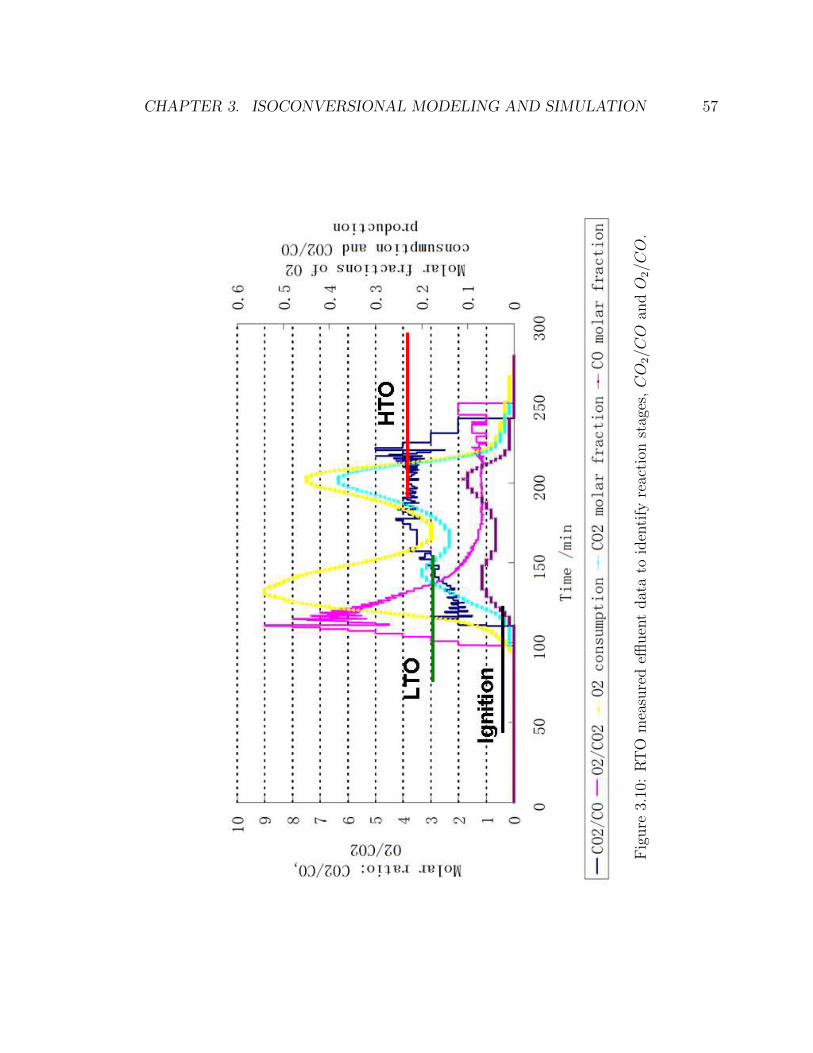
CHAPTER 3. ISOCONVERSIONAL MODELING AND SIMULATION 57
Fig
ure
3.10
:R
TO
mea
sure
deffl
uen
tdat
ato
iden
tify
reac
tion
stag
es,CO
2/CO
andO
2/CO
.

CHAPTER 3. ISOCONVERSIONAL MODELING AND SIMULATION 58
Fig
ure
3.11
:Is
oco
nve
rsio
nal
finge
rpri
nts
for
the
four
set
ofR
TO
exp
erim
ents
usi
ng
diff
eren
tox
yge
nco
mp
osit
ions
inin
ject
ion
gas
stre
am.
The
35%
oxyge
nca
sedoes
not
show
consi
sten
tb
ehav
ior
asth
eot
her
thre
eca
ses.
Itis
not
use
dfo
rth
eox
yge
nre
acti
onor
der
inte
rpre
tati
on.

CHAPTER 3. ISOCONVERSIONAL MODELING AND SIMULATION 59
050
100
150
200
250
300
−0.
10
0.1
0.2
0.3
0.4
0.5
0.6
0.7
0.8
Tim
e /m
in
Gas consumption, molar percentage
Mea
sure
d O
2M
easu
red
CO
Mea
sure
d C
O2
Sim
ulat
ed O
2S
imul
ated
CO
Sim
ulat
ed C
O2
Fig
ure
3.12
:V
KC
sim
ula
tion
resu
lts
bas
edon
the
init
ial
inte
rpre
tati
onfo
rva
lues
ofac
tiva
tion
ener
gy,
reac
tion
order
s,an
dpre
-exp
onen
tial
fact
orsA
.
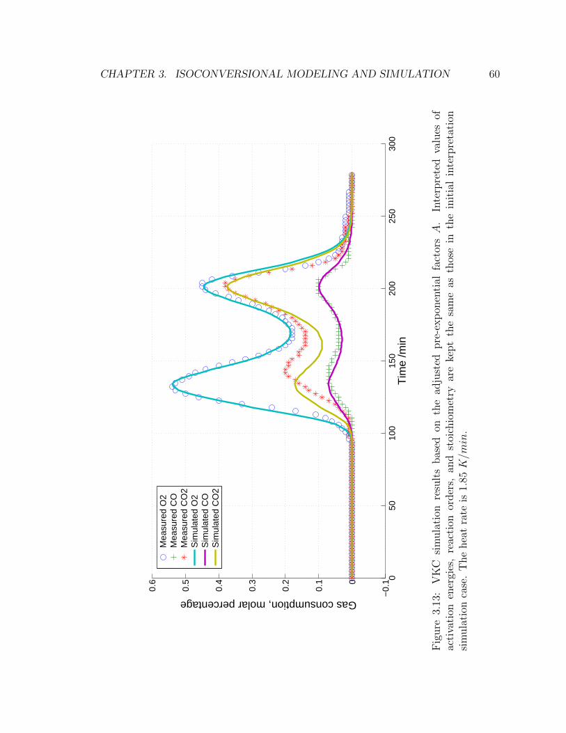
CHAPTER 3. ISOCONVERSIONAL MODELING AND SIMULATION 60
050
100
150
200
250
300
−0.
10
0.1
0.2
0.3
0.4
0.5
0.6
Tim
e /m
in
Gas consumption, molar percentage
Mea
sure
d O
2M
easu
red
CO
Mea
sure
d C
O2
Sim
ulat
ed O
2S
imul
ated
CO
Sim
ulat
ed C
O2
Fig
ure
3.13
:V
KC
sim
ula
tion
resu
lts
bas
edon
the
adju
sted
pre
-exp
onen
tial
fact
orsA
.In
terp
rete
dva
lues
ofac
tiva
tion
ener
gies
,re
acti
onor
der
s,an
dst
oich
iom
etry
are
kept
the
sam
eas
thos
ein
the
init
ial
inte
rpre
tati
onsi
mula
tion
case
.T
he
hea
tra
teis
1.85
K/m
in.

CHAPTER 3. ISOCONVERSIONAL MODELING AND SIMULATION 61
0 50 100 150 200 250 3000
100
200
300
400
500
600
Time /min
Tem
pera
ture
/C
RTO measurementVKC Simulation
Figure 3.14: Temperature history comparison between the VKC simulation resultRTO measurement. The heat rate is 1.85 K/min
0 0.2 0.4 0.6 0.8 10
0.5
1
1.5
2
x 105
Conversion
Act
ivat
ion
Ene
rgy,
J/m
ole RTO experiment
Simulation
Figure 3.15: Isoconversional fingerprint comparison between the VKC simulationresult and RTO measurement.

CHAPTER 3. ISOCONVERSIONAL MODELING AND SIMULATION 62
Table 3.5: Comparison between initial and adjusted values of pre-exponential factorfor the Alaska crude-oil combustion modeling.
Initially estimated, 1/(mole ·min) Adjusted, 1/(mole ·min)
LTO 3.69× 10¹⁵ 1.5× 10¹⁵
HTO 9.95× 10¹³ 1.6× 10¹⁴
Table 3.6: Kinetic parameters for the proposed model of the Alaska crude-oil com-bustion.
Reaction A, 1/(mole ·min) Ea, J/mole ∆H, J/mole a b
Ignition 1.0× 10¹⁰ 1.0× 10⁵ 3.6× 10⁶ – 1LTO 1.5× 10¹⁵ 8.5× 10⁴ 1.86× 10⁷ 0.9 1.83HTO 1.6× 10¹⁴ 1.3× 10⁵ 1.0× 10⁶ 1.0 1.45
3.3.4 Karamay oil sample
The same modeling procedure is conducted for the Karamay crude-oil (11.8 ◦API)
combustion. The crude-oil /reservoir-sand mixture of 15 gram is used for each of
the RTO experiments. The composition is of 2.04 wt% crude oil, 8.16 wt% water,
and 89.8 wt% sand matrix. 0.31 gram of crude oil is initially within the kinetic cell.
The gas injection rate is set to be 1.5 L/min at the standard condition (25 ◦C and
1.01325 × 10⁵ Pa). The RTO effluent data shown in Figure 3.16 with the heat rate
of 1.85 K/min is used for the stoichiometry calculation.
The first step is defining the stoichiometry for the HTO reaction in Scheme 3.24.
From Figure 3.16, CO2/CO is 8.1, O2/CO2 is 1.1. Using mass balance, H2O/CO2
is 0.067 and H/C is 0.119. With these information, the chemical formula for coke is
CH0.119, and the stoichiometry for the HTO reaction is calculated by the balance of
elements.
The entire reaction period of the RTO experiment is 18600 seconds. Processing
the integral of the production gas of both CO and CO2 over the reaction period, an
amount of 1.32× 10⁻² mole of carbon C is captured by the gas analyzer in the form
of carbon oxides. Considering the oxygen consumption contributes to the production

CHAPTER 3. ISOCONVERSIONAL MODELING AND SIMULATION 63
of carbon oxides and water, the apparent hydrogen content within the crude-oil is
calculated by subtracting oxygen in carbon oxides, and it is 2.81× 10⁻² mole. Thus,
a total mass of carbon and hydrogen from crude-oil that is involved in reactions
recorded by the gas analyzer is 0.19 gram. The mass difference between the initial
crude-oil and total mass of carbon and hydrogen recorded by the gas analyzer is
caused by volatile components of the crude oil or other produced hydrocarbon gas
that can not be recognized by the gas analyzer. Based on mass balance, 60.95% of
the original crude oil reacts with oxygen and generates coke, carbon oxides and water,
and the other 39.05% is grouped into V C. From Figure 3.10, in the LTO stage, the
ratio of CO2 and CO is 2.8, and O2/CO2 is around 3.4. The crude oil molecular
weight is estimated by adjusting its value to match the peak oxygen consumption of
either LTO or HTO, and it is 455 g/mole. The molar ratio of O2 and the coke is
estimated by the peak oxygen consumption ratio of LTO and HTO. H2O can not be
estimated from the measurement, so it is used to balance the mass of products for
the LTO reaction. The proposed reaction scheme for Karamay crude-oil mixture is:
Oilk1−→ Oil∗ (Ignition)
Oil∗ + 15.5O2k2−→ 13.5CH0.119 + 5.6CO2 + 2.03CO + 17.03H2O + 6.34V C (LTO)
CH0.119 + 0.98O2k3−→ 0.89CO2 + 0.11CO + 0.06H2O (HTO)
Reaction scheme 3.26
After defining the stoichiometry, kinetic parameters for each of the reactions are
interpreted. Three sets of RTO experiments using different oxygen composition in
the gas injection are carried out. The three activation energy fingerprints are plotted
in Figure 3.17. The 35% oxygen case does not reveal consistent fingerprint as those
with oxygen compositions of 16.6% and 20.7%. So the 35% oxygen case is not taken
into consideration for parameter interpretation. The ignition reaction take places at
the very begining. From Figure 3.11, the activation value for the ignition reaction
is about 1.13 × 10⁵ J/mole. The pre-exponential factor can be estimated from the
starting point of oxygen consumption and A is 3.7 × 10¹⁰ 1/(mole · min). For the

CHAPTER 3. ISOCONVERSIONAL MODELING AND SIMULATION 64
Table 3.7: Kinetic parameters for proposed model of the Karamay crude-oil combus-tion
Reaction A, 1/(mole ·min) Ea, J/mole ∆H, J/mole a b
Ignition 3.7× 10¹⁰ 1.13× 10⁵ 2.6× 10⁶ – 1LTO 1.0× 10¹⁵ 7.5× 10⁴ 1.96× 10⁷ 1.3 0.92HTO 4.2× 10¹² 1.0× 10⁵ 1.3× 10⁶ 0.9 1.41
LTO reaction, the activation energy is about 7.5 × 10⁴ J/mole. Two conversion X
values, 0.2 and 0.25, are chosen to process the calculation for the fuel reaction order.
The RTO experiments used are the ones with air injection. The LTO reaction begins
at about X = 0.1 and ends at around X = 0.6. Based on Eq. 3.13, the LTO reaction
order for fuel is b = 0.92. Calculating the oxygen partial pressure reaction order, the
conversion value of 0.2 is used for RTO experiments of different oxygen compositon
in the injection gas. Based on Eq. 3.17, the reaction order for oxygen is a = 1.3. The
same interpretation for HTO reaction parameters is conducted. The HTO activation
energy is interpreted from Figure 3.11 and it is around 1.0 × 10⁵ J/mole. Two
conversion X values, 0.7 and 0.75, are chosen to process the calculation for the fuel
reaction order and b = 1.41. the conversion value of 0.7 is used to interpret the HTO
oxygen reaction order and a = 0.9. After adjusting pre-exponential factors based
on the intial guess by Eq. 3.18, the kinetic parameters for the Karamay crude-oil
combustion are listed in Table 3.7.
The simulation result based on the kinetic model listed in Table 3.7 is shown in
Figure 3.18. The simulation represents very good matches with the effluent gas data.
The simulations also show very good match of the temperature history in Figure 3.19.
When comparing the isoconversional fingerprints interpreted from RTO experiments
and simulation in Figure 3.20, the simulated fingerprint has a very similar behavior
as the RTO experiments.

CHAPTER 3. ISOCONVERSIONAL MODELING AND SIMULATION 65
Fig
ure
3.16
:R
TO
mea
sure
deffl
uen
tdat
ato
iden
tify
reac
tion
stag
es,CO
2/CO
andO
2/CO
.

CHAPTER 3. ISOCONVERSIONAL MODELING AND SIMULATION 66
Fig
ure
3.17
:Is
oco
nve
rsio
nal
finge
rpri
nts
for
the
thre
ese
tof
RT
Oex
per
imen
tsusi
ng
diff
eren
tox
yge
nco
mp
osit
ions
inth
ein
ject
ion
gas
stre
am.
The
35%
oxyge
nca
sedoes
not
show
consi
sten
tb
ehav
ior
asth
eot
her
thre
eca
ses.
Itis
not
use
dfo
rth
eox
yge
nre
acti
onor
der
inte
rpre
tati
on.

CHAPTER 3. ISOCONVERSIONAL MODELING AND SIMULATION 67
050
100
150
200
250
300
350
−0.
10
0.1
0.2
0.3
0.4
0.5
0.6
0.7
0.8
Tim
e /m
in
Gas consumption, molar percentage
Mea
sure
d O
2M
easu
red
CO
Mea
sure
d C
O2
Sim
ulat
ed O
2S
imul
ated
CO
Sim
ulat
ed C
O2
Fig
ure
3.18
:V
KC
sim
ula
tion
resu
lts
bas
edon
the
adju
sted
pre
-exp
onen
tial
fact
orsA
.In
terp
rete
dva
lues
ofac
tiva
tion
ener
gies
,re
acti
onor
der
s,an
dst
oich
iom
etry
are
kept
the
sam
eas
thos
ein
the
init
ial
inte
rpre
tati
ons:
The
hea
tra
teis
1.85
K/m
in.

CHAPTER 3. ISOCONVERSIONAL MODELING AND SIMULATION 68
0 100 200 300 4000
100
200
300
400
500
600
700
Time /min
Tem
pera
ture
/C
RTO measurementVKC Simulation
Figure 3.19: Temperature history comparison between the VKC simulation resultRTO measurement: the heat rate is 1.85 K/min
0 0.2 0.4 0.6 0.8 10
0.5
1
1.5
2
x 105
Conversion
Act
ivat
ion
Ene
rgy,
J/m
ole RTO experiment
Simulation
Figure 3.20: Isoconversional fingerprint comparison between the VKC simulationresult RTO measurement.

CHAPTER 3. ISOCONVERSIONAL MODELING AND SIMULATION 69
3.4 Discussion
The proposed method combines the isoconversional and conventional principles to-
gether to interpret kinetic parameters, activation energy, pre-exponential factor and
reaction orders, for reaction model from RTO experiments. The synthetic cases of
unit and non-unit reaction orders exhibit very good matches between the model val-
ues and the interpreted values of kinetic parameters. The method is applied to build
reaction models for two different crude-oil/sand mixtures. A three-reaction scheme
is proposed based on reaction stages identified from isoconversional fingerprint as
well as RTO effluent data. Stoichiometry is defined from effluent data, activation
energy is read from the isoconversional fingerprint, reaction orders are interpreted by
processing several sets of RTO experiments using different oxygen compositions in
the injection gas stream, and pre-exponential factor is given as an initial guess and
then adjusted to match the measurement. The virtual kinetic cell simulation coupled
with the proposed model well represents the combustion performance of the crude
oil mixture within the kinetic cell, regarding the temperature histories, effluent gas
histories, and the isoconversional fingerprint.
The proposed three-reaction scheme captures major characteristics of crude-oil
combustion. Improvement of the proposed scheme is needed to make the simulations
match the ignition stage with respect to carbon oxides, and transition stage between
LTO and HTO in terms of oxygen profiles. Adding more reactions, such as four or five
reactions, to the reaction scheme would make simulations more accurate. Also, adding
an intermediate reactant, such as a coke component burned at the LTO stage [17]
would improve the transition stage on the isoconversional fingerprint. The additions
of reactions or reactants makes the interpretation more complicated, so more work is
needed to improve the interpretation method combining the isoconversional principle
and conventional methods.
For the 35% oxygen composition cases, eight experiments have been done, in total.
Four each for Alaskan and Karamay crude oil cases. The measurement data are shown
in Figure 3.21 and 3.22 for the Alaskan and the Karamay crude oil respectively. From
the temperature and the effluent gas profiles, they represent very good trends and

CHAPTER 3. ISOCONVERSIONAL MODELING AND SIMULATION 70
a certain degree of consistency. The consistency check (ln(dx/dt) vs. −1/RT ), as
discussed in Chapter 2, gives poor results showing in Figure 3.23 and 3.24, especially
for the Karamay crude oil case. The consistency check for the Alaskan case shows poor
consistency in the transition zone between LTO and HTO stages, and for the Karamay
case, the consistency check suggests that RTO measurements are not consistent at
all.

CHAPTER 3. ISOCONVERSIONAL MODELING AND SIMULATION 71
(a) Temperature histories
(b) Oxygen consumption histories
Figure 3.21: Alaskan crude oil RTO experiments: 35% oxygen composition.

CHAPTER 3. ISOCONVERSIONAL MODELING AND SIMULATION 72
(a) Temperature histories
(b) Oxygen consumption histories
Figure 3.22: Karamay crude oil RTO experiments: 35% oxygen composition.

CHAPTER 3. ISOCONVERSIONAL MODELING AND SIMULATION 73
Figure 3.23: Consistency check for the 35% oxygen composition RTO experiments ofAlaskan crude oil.
Figure 3.24: Consistency check for the 35% oxygen composition RTO experiments ofKaramay crude oil.

Chapter 4
Isoconversional application
The isoconversional principle has strong power to categorize the reaction kinetics
within crude-oil combustion in terms of the activation energy fingerprint. The iso-
conversional fingerprint inherently contains abundant kinetic information. Different
reaction stages such as LTO and HTO are clearly identified. Kinetic parameters (acti-
vation energy, pre-exponential factor and reaction orders) are interpreted for reaction
modeling. In this chapter, the isoconversional fingerprint is used as a qualitative
analysis tool to investigate detailed aspects in the ISC process. It is applied to ana-
lyze sand and clay surface area effects on ISC kinetics, coke formation under different
conditions, and to screen the crude-oil/rock-matrix pair for potential ISC candidates.
4.1 Reservoir matrix effect
Many researchers have shown that sand and clay surface area have a significant effect
on crude-oil combustion [111][25][18][47][49]. The addition of clay to the rock matrix
enhances the crude-oil combustion by reduction of activation energy. Large surface
area and metallic catalytic components of the clay contribute to the enhancement.
Vossoughi et al. [110] showed that a combustion tube run of sand/crude-oil mixture
failed to achieve combustion front propagation, while a strong self-sustained com-
bustion front was formed when mixing a certain amount of clay with the sand. In
another study, Cinar et al. [18] mixed a crude oil with sand of different grain sizes:
74

CHAPTER 4. ISOCONVERSIONAL APPLICATION 75
Table 4.1: Crude-oil/rock matrix pairs for RTO experiments
Alaskan crude oil Case 1 60 mesh fired sand + clayCase 2 60 mesh fired sandCase 3 12 mesh sand
Karamay crude oil Case 1 reservoir sandCase 2 60 mesh fired sand + clayCase 3 60 mesh fired sand
sand crushed from reservoir rock (about 10 to 16 mesh) and artificial sand of 60 mesh,
and did the combustion tube run. A sustained combustion propagation was observed
for the crude oil mixed with 60 mesh sand case. The other one with larger grain size,
crushed reservoir rock could not form a propagating temperature front.
Surface area alters the heat conductivity behavior of porous media. Both catalytic
effect and surface area influence the reaction paths of the crude-oil combustion, and
thus the apparent activation energy. Isoconversional fingerprint exhibits the activa-
tion energies as a function of oxygen conversion. Rock matrix effect on the reaction
kinetics can be investigated by analyzing the fingerprint interpreted from RTO exper-
iments. Two sets of experiments are conducted using Alaskan crude oil and Karamay
crude oil. The crude oil and rock matrix conditions for the RTO experiments are
listed in Table 4.1:
4.1.1 Alaskan crude-oil cases
The Alaskan crude-oil has an API of 13.3. Three cases of different sand matrix are
considered. They are case 1 with 60 mesh fired sand and clay, case 2 with 60 mesh
fired sand and case 3 with 12 mesh fired sand. 25 grams of the sand/crude-oil mixture
is used in the kinetic cell. The size of the sample for a RTO experiment is defined by a
series of RTO tests with different sample sizes so that temperature deviations during
LTO and HTO are small enough to make the measurement consistent. The sample
size still needs to be large enough to acquire precise effluent gas measurement. 1.5
L/min air injection rate is used for each case. The RTO measurements of temperature

CHAPTER 4. ISOCONVERSIONAL APPLICATION 76
Table 4.2: Oxygen consumption comparison of LTO and HTO for Alaskan crude oilcases
Peak oxygen Amount of oxygenconsumption ratio consumption ratio
Case 1 1.16 1.86Case 2 0.81 1.33Case 3 0.41 0.67
histories as well as oxygen consumption profiles for each experimental case are plotted
in Figure 4.1, 4.2, and 4.3 respectively.
Case 1 with clay in Figure 4.1 exhibits very different oxygen consumption behavior
from those in both case 2 and case 3, where only the sand of different grain size is
mixed with crude oil. The presence of clay significantly enhances the first oxygen
consumption hump, that is the low temperature oxidation regime. The enhancement
in the LTO reaction stage increases the amount of fuel laid down. Fuel laid down is
a critical parameter to evaluate the capability of a self-sustaining combustion front
propagation. When the crude oil was mixed with sand only, case 2 and case 3 both
show the oxygen consumption peak in LTO is much lower than that of HTO. This
means that in the entire combustion process, a large portion of reactions occur at the
high temperature regime. Comparing the peak oxygen consumption ratio of LTO and
HTO in case 2 and case 3, case 2 has more oxygen consumption in LTO than that of
case 3. Case 2 uses fired sand of 60 mesh, and it has larger surface area than the sand
of 12 mesh used in case 3. Both cases do not have clay involved. The comparison of
oxygen consumption of the three cases are listed in Table 4.2.
When using isoconversional fingerprints to compare the three cases in Figure 4.4,
the same conclusion is also made that the clay addition in case 1 much enhances the
LTO in terms of amount ratio of oxygen consumption in LTO and HTO, and surface
effect is more favorable when using sands of smaller grain size (Table 4.2). When
this goes to the kinetic analysis, comparison of the activation energy values in LTO
and HTO for the three cases is very close. The LTO activation energies are between
0.7×10⁵ and 0.8×10⁵ J/mole, and the HTO activation energies are roughly 1.2×10⁵

CHAPTER 4. ISOCONVERSIONAL APPLICATION 77
0 50 100 150 200 250 300 350 400200
300
400
500
600
700
800
900
Time,min
Tem
pera
ture
, K
2.64 K/min
1.93 K/min
1.74 K/min
1.54 K/min
(a) Temperature histories
0 50 100 150 200 250 300 350 4000
0.1
0.2
0.3
0.4
0.5
0.6
0.7
0.8
0.9
Time,min
O2 c
onsu
mpt
ion,
Mol
e fr
actio
n
2.64 K/min1.93 K/min1.74 K/min1.54 K/min
(b) Oxygen consumption histories
Figure 4.1: Alaskan crude oil case 1: 60 mesh fired sand and clay; 25g mixture of2.04 wt% crude oil, 8.16 wt% water, 81.63 wt% fired sand and 8.16 wt% clay; Airinjection rate is 1.5 L/min.

CHAPTER 4. ISOCONVERSIONAL APPLICATION 78
0 50 100 150 200 250 300 350 400200
300
400
500
600
700
800
900
Time,min
Tem
pera
ture
, K
2.64 K/min
2.10 K/min
1.76 K/min
1.51 K/min
(a) Temperature histories
0 50 100 150 200 250 300 350 4000
0.2
0.4
0.6
0.8
1
1.2
1.4
Time,min
O2 c
onsu
mpt
ion,
Mol
e fr
actio
n
2.64 K/min2.10 K/min1.76 K/min1.51 K/min
(b) Oxygen consumption histories
Figure 4.2: Alaskan crude oil case 2: 60 mesh fired sand; 25g mixture of 2.04 wt%crude oil, 8.16 wt% water, 89.90 wt% fired sand; Air injection rate is 1.5 L/min.

CHAPTER 4. ISOCONVERSIONAL APPLICATION 79
0 50 100 150 200 250 300 350 400200
300
400
500
600
700
800
900
Time,min
Tem
pera
ture
, K
2.20 K/min
1.84 K/min
1.60 K/min
(a) Temperature histories
0 50 100 150 200 250 300 350 4000
0.1
0.2
0.3
0.4
0.5
0.6
0.7
0.8
0.9
Time,min
O2 c
onsu
mpt
ion,
Mol
e fr
actio
n
2.20 K/min1.84 K/min1.60 K/min
(b) Oxygen consumption histories
Figure 4.3: Alaskan crude oil case 3: 12 mesh fired sand; 25g mixture of 2.04 wt%crude oil, 8.16 wt% water, 89.90 wt% fired sand; Air injection rate is 1.5 L/min.

CHAPTER 4. ISOCONVERSIONAL APPLICATION 80
and 1.3× 10⁵ J/mole. The LTO region shows a flat plateau for all of the three cases,
but the shapes of the HTO plateau are very different. Case 1 with clay addition
shows a flat plateau in the HTO regime, while case 2 and case 3 show a flat HTO
plateau at the beginning but the activation energy increases after the flat region.
The increased apparent activation energies are due to some kind of coke residual with
greater activation energies. Case 2 and 3 need more energy and higher temperature
to burn all of the HTO residues than case 1 with a flat HTO region all the way to
X = 1.
Besides the interesting LTO and HTO kinetic behaviors in different porous media
cases, the negative temperature gradient region (NTGR) is clearly detected in case
2 and case 3 where no clay is present in the matrix. The NTGR is also referred as
’Death Valley’ [22] where oxygen uptake decreases while temperature is still increased
[70]. The exist once of the NTGR challenges the sustainability of the ISC due to the
decrease in the reaction rate. Insufficient heat released from reactions to support high
temperature when the reaction rate goes down according to the rate law. Cinar et al.
[16][16][17] first investigated the NTGR character by using isoconversional fingerprint
and described it using the cool flame theory: an incomplete combustion associated
with the NTGR where oxygen uptake as well as heat released, decrease with increasing
temperature. On an isoconversional fingerprint, NTGR exists in between the LTO
and HTO regions where a local minimum activation energy is reached.
For case 2, the NTGR is located at the conversion region of 0.35 to 0.5, with a
minimum activation energy value of 0.5× 10⁵ J/mole, while in the case 3 with larger
sand grain size and smaller matrix surface area, the NTGR happens in the conversion
region of 0.25 to 0.35 and the smallest activation energy value is about 0.22 × 10⁵
J/mole. This means that case 2 more easily forms a good combustion front with
a shallow NTGR and later location of it, as compared to case 3 in which sand of
larger grain size is used. There is no apparent NTGR observed in case 3 where clay is
mixed with the crude-oil sample. The comparison of fingerprints of the three Alaskan
cases clearly demonstrates the differences in the reaction kinetic behavior of crude oil
coupled with different porous media. The existence of NTGR retards the combustion
propagation, while the clay addition removes the NTGR in the reaction path and

CHAPTER 4. ISOCONVERSIONAL APPLICATION 81
enhances crude oil combustion.
0 0.2 0.4 0.6 0.8 10
0.2
0.4
0.6
0.8
1
1.2
1.4
1.6
1.8
2
2.2x 10
5
Conversion
Act
ivat
ion
Ene
rgy,
J/m
ole 60 mesh fired sand + clay
60 mesh fired sand12 mesh sand
Figure 4.4: Activation energy fingerprints comparison for Alaskan crude oil cases.
4.1.2 Karamay crude-oil cases
Another three sets of RTO experiments were carried out using the Karamay crude
oil sample with 11.8 ◦API. The sand matrix compositions are listed in Table 4.1 for
each case. The sample mixture for each case has a composition of 2.04 wt% crude
oil, 8.16 wt% water, 89.90 wt% sand matrix and the air injection rate is 1.5 L/min.
Case 1 is conducted with a sample mixture of real reservoir sand. The reservoir sand
has finer grain size than the fired sand of 60 mesh and contains a certain amount the
clay with metalic species. Case 2 is carried with 60 mesh fired sand and clay, case 3
with 60 mesh fired sand only.

CHAPTER 4. ISOCONVERSIONAL APPLICATION 82
Table 4.3: Oxygen consumption comparison of LTO and HTO for Karamay crude oilcases
Peak oxygen Amount of oxygenconsumption ratio consumption ratio
Case 1 2.83 1.86Case 2 3.31 1.86Case 3 1.72 1.63
RTO measurements of temperature histories as well as oxygen consumption histo-
ries for the three cases are plotted in Figure 4.5, 4.6, and 4.7 respectively. The oxygen
consumption histories for all of the three case shows similar performance that LTO
region consumes more oxygen than the HTO region. Comparison of oxygen consump-
tions based on oxygen uptake histories for the three cases are listed in Table 4.3. The
LTO region is enhanced in both case 1 and case 2 where the porous media contains
clay. The same kinetic analysis is done to Karamay cases using the isoconversional
fingerprint. The three activation energy fingerprints are very different from each other
in both LTO and HTO regions. In the LTO region, case 1 and case 2 have smaller
activation energy values than case 3. In the HTO region, case 3 of no clay addition
shows the highest activation energy values and has an increasing trend of activation
energies when the combustion approaches to the end. Case 2 has a smaller activation
energy values in the HTO region than case 3, greater values than case 1, but there
is very little increasing trend in activation energies. The clay addition to the sample
mixture contributes to the decrease of activation energies in case 2. The same clay
effect is seen in the HTO region of case 1, where a flat activation energy plateau is
formed. Analyzing the reaction region in between the LTO and HTO stages, case 3
without clay addition formed an obvious NTGR, which holds a minimum activation
energy value around 0.5 × 10⁵ J/mole. Case 1 and Case 2 also have a NTGR-like
shape in between the LTO and HTO region, but the minimum activation energy val-
ues of it are very close to that of the early stage of the LTO region. Overall, case 1
with the reservoir sand has the smoothest fingerprint regarding the difference between
the maximum and minimum activation energies, case 2 with the fired sand and clay

CHAPTER 4. ISOCONVERSIONAL APPLICATION 83
0 50 100 150 200 250 300 350200
300
400
500
600
700
800
900
Time,min
Tem
pera
ture
, K
2.65 K/min
2.15 K/min
1.81 K/min
1.54 K/min
(a) Temperature histories
0 50 100 150 200 250 300 3500
0.2
0.4
0.6
0.8
1
1.2
1.4
Time,min
O2 c
onsu
mpt
ion,
Mol
e fr
actio
n
2.65 K/min2.15 K/min1.81 K/min1.54 K/min
(b) Oxygen consumption histories
Figure 4.5: Karamay crude oil case 1: reservoir sand; 15g mixture of 2.04 wt% crudeoil, 8.16 wt% water, 89.90 wt% fired sand; Air injection rate is 1.5 L/min.

CHAPTER 4. ISOCONVERSIONAL APPLICATION 84
0 50 100 150 200 250 300 350200
300
400
500
600
700
800
900
Time,min
Tem
pera
ture
, K
2.59 K/min
2.10 K/min
1.73 K/min
1.53 K/min
(a) Temperature histories
0 50 100 150 200 250 300 3500
0.2
0.4
0.6
0.8
1
1.2
1.4
1.6
1.8
2
Time,min
O2 c
onsu
mpt
ion,
Mol
e fr
actio
n
2.59 K/min2.10 K/min1.73 K/min1.53 K/min
(b) Oxygen consumption histories
Figure 4.6: Karamay crude oil case 2: 60 mesh fired sand and clay; 25g mixture of2.04 wt% crude oil, 8.16 wt% water, 81.63 wt% fired sand and 8.16 wt% clay; Airinjection rate is 1.5 L/min.

CHAPTER 4. ISOCONVERSIONAL APPLICATION 85
0 50 100 150 200 250 300 350300
400
500
600
700
800
900
Time,min
Tem
pera
ture
, K
2.57 K/min
2.09 K/min
1.77 K/min
1.52 K/min
(a) Temperature histories
0 50 100 150 200 250 300 3500
0.2
0.4
0.6
0.8
1
1.2
1.4
Time,min
O2 c
onsu
mpt
ion,
Mol
e fr
actio
n
2.57 K/min2.09 K/min1.77 K/min1.52 K/min
(b) Oxygen consumption histories
Figure 4.7: Karamay crude oil case 3: 60 mesh fired sand; 25g mixture of 2.04 wt%crude oil, 8.16 wt% water, 89.90 wt% fired sand; Air injection rate is 1.5 L/min.

CHAPTER 4. ISOCONVERSIONAL APPLICATION 86
0 0.2 0.4 0.6 0.8 10
0.2
0.4
0.6
0.8
1
1.2
1.4
1.6
1.8
2
2.2x 10
5
Conversion
Act
ivat
ion
Ene
rgy,
J/m
ole Reservoir sand
60 mesh fired sand + clay60 mesh fired sand
Figure 4.8: Activation energy fingerprints comparison for Karamay crude oil cases.
addition enhances the combustion in both LTO and HTO regions. Case 1 and case 2
have more favorable combustion behavior than case 3 because of larger surface and
clay addition.
Based on the two crude oil samples and six RTO experiments with different porous
media, the conclusion is drawn that surface area and clay effect of porous media has
significant impacts on the activation energy for the whole combustion process. The
isoconversional fingerprint is very useful to demonstrate the changes in the reaction
paths and to identify reaction regimes, such as LTO, HTO, and NTGR.

CHAPTER 4. ISOCONVERSIONAL APPLICATION 87
4.2 Coke formation investigation
In the low temperature oxidation (LTO) region, series and parallel reactions [17], in-
cluding dehydrogenation, cracking, and condensation, produce a carbonacesus residue
on the surface of porous media. The carbonaceous residue, also referred to as coke, is a
kind of solid hydrocarbon components insoluble in toluene. The heavy fraction of the
crude oil, asphaltenes, is the major source to produce coke composition during ISC.
The LTO reactions increase the content of asphaltene while decreasing the content of
resin [73]. When crude oil reacts under an inert gas condition like nitrogen, coke is
formed after an induction period under the isothermal condition of 673 K [117]. On
the other hand, when under air flow condition, coke is formed immediately when the
temperature goes up [17]. The amount of coke formation is a critical index for the
quantity of fuel available for a self-sustainable combustion: excessive fuel deposition
consumes too much crude oil and oxygen, making the advance of the combustion
front very slow and the production not economical, while insufficient fuel deposition
may not provide enough heat to maintain a self-sustained combustion process.
Wiehe et al. [117] used an isothermal batch reactor to study coke formation under
nitrogen and air conditions, reporting different induction time for coke formation.
Cinar et al. [17] followed Wiehe’s way to produce coke in a quartz tube reactor under
isothermal condition. They investigated two kinds of coke formed under nitrogen
flow and air flow. A conclusion similar to Wiehe’s is gained that coke is formed
immediately under the air flow condition at atmospheric pressure and at 673 ◦C,
while under the nitrogen flow condition, a 45 min induction period is needed to
produce a significant amount of coke. XPS for coke surface scanning indicates oxygen
functional groups exist on the surface of coke precipitated under air flow condition.
A stainless steel isothermal kinetic cell (KC) shown in Figure 4.9 is designed for
coke formation under different gas flow condition. The isothermal KC has a stainless
steel body that is 2.5 cm in diameter and 12 cm in length. Swagelock fittings are used
to seal both ends of the cell. Gas is preheated initially and then injected through
the bottom fitting. A thermal well is inserted to the center of the cell to record
temperatures. Production gases travel through the production well in the top fitting.

CHAPTER 4. ISOCONVERSIONAL APPLICATION 88
Comparing to the quartz tube reactor [17], the stainless steel isothermal KC can
operate at elevated temperature. Meanwhile, production gas is conducted to the gas
analyzer so that the progress of a isothermal experiment is monitored and precise
control is managed.
The coke formation investigation follows Cinar’s method [17] and improvements on
the workflow are introduced. A certain amount of crude-oil/sand mixture is padded
into the KC. Pressure is elevated with gas injection till it reaches the prescribed
pressure condition (normally 100 psi is applied). The isothermal KC is put in the
furnace with a pre-set constant temperature. The long tube conducts heat from the
furnace to preheat injection gas. Temperature and effluent gas data are recorded
and monitored to determine when to quench the experiment. When the set time is
reached, the isothermal KC is taken outside the furnace and cold water is sprayed
immediately until the KC temperature goes under 40 ◦C. The formation coke is taken
out for toluene extraction, and then it is dried out overnight in the vacuum oven. The
experiments are repeated until enough coke is made for further XPS analysis and RTO
experiments. XPS analysis is conducted to analyze chemical functional groups on the
coke surface. RTO experiments are carried out to get the isoconversional fingerprint
for the coke activation energies.
A mixture of Karamay crude-oil and the reservoir sand is used. The mixture
composition is of 2.04 wt% crude oil, 8.16 wt% water and 89.90 wt% reservoir sand.
Exactly 45 grams of the mixture is used for each experiment. The pressure within the
kinetic cell is 100 psi that is the same as that used in RTO experiments. Two kinds
of coke, one formed under the air flow condition and the other under the nitrogen
flow condition, are investigated.
4.2.1 Coke formed under air
The coke formed in the LTO stage is the major fuel for the HTO burning. Its reaction
kinetics controls the heat releasing which is essential to support the combustion front
propagation. Adegbesan et. al. [2] proposed a reaction scheme for LTO (Reaction
scheme 4.1), that includes the reaction paths to generate coke during the LTO period.

CHAPTER 4. ISOCONVERSIONAL APPLICATION 89
Figure 4.9: The kinetic cell for coke formation study in the isothermal condition.
Maltenes+O2k1−→ Asphaltenes (4.1a)
Asphaltenes+O2k2−→ Coke (4.1b)
The first attempt of the coke investigation is to determine the constant temper-
ature value used in the isothermal experiment through an RTO experiment. The
result of which is shown in Figure 4.10. The termination temperature value should
be below the temperature triggering the HTO reactions and high enough to make
LTO reaction progress quickly. According to the RTO experiment result in Figure
4.10, LTO starts at around 200 ◦C and terminates at around 330 ◦C. So 300 ◦C is
selected for isothermal experiments.
The air injection rate of 2 L/min is used for the isothermal experiments. In total,
four experiments are carried out with a sample mixture of 45 g for each. Temperatures
and effluent gas data are shown in Figure 4.11. A temperature of 300 ◦C is set as
the constant temperature for the furnace. The mixture within the kinetic cell is
heated up to 283 ◦C in about 45 minutes and then the temperature is kept constant.

CHAPTER 4. ISOCONVERSIONAL APPLICATION 90
Figure 4.10: Defining the termination temperature for the isothermal experiment ofair coke formation: 300 ◦C is selected.
The temperature gap is caused by the heat balance within the kinetic cell. Oxygen
consumption is increased with the elevated temperature. The constant temperature
of 283 ◦C is kept until LTO is nearly finished, that is oxygen consumption approaches
a plateau in about 105 minutes. The kinetic cell is taken out of the furnace quickly
and water is sprayed to cool it down immediately. Temperature drops from 283 ◦C
to about 40 ◦C in 5 minutes. Oxygen consumption goes to zero when the kinetic
cell is cooled down. Coke is collected from four experiments, crushed to make a
homogeneous mixture and then cleaned by toluene to extract heavy residues of crude-
oil. The coke is dried by placing it in the vacuum cell for 2 days and then it is ready
for further investigation.
The kinetic analysis of the coke combustion is studied by RTO experiments and
isoconversional interpretation. A coke mixture of 30 gram is put into the conventional
kinetic cell. An air injection rate of 1.5 L/min is used. Four RTO experiments are
conducted and temperature and effluent gas histories are shown in Figure 4.12. The
oxygen consumption presents only one hump during the ramped temperature process,
because LTO reactions are nearly finished in the isothermal experiments and residual

CHAPTER 4. ISOCONVERSIONAL APPLICATION 91
Figure 4.11: Coke is formed in the isothermal experiments.
heavy components are removed by toluene, only coke which is the major fuels for
HTO reacts with oxygen in RTO experiments. The isoconversional fingerprint in
Figure 4.13(a) presents a flat plateau of activation energy values, which supports
the argument that one lumped reaction is enough to described the reaction kinetics
for coke combustion. When the activation energy values in Figure 4.13(a) compared
with those in the HTO stage of the entire crude-oil combustion shown in Figure
4.13(b), they match each other fairly well. The interesting result strongly supports
the capability of isoconversional principle for deconvolving the multi-step reaction
mechanism for crude-oil combustion.

CHAPTER 4. ISOCONVERSIONAL APPLICATION 92
0 50 100 150 200 250 300 350 400200
300
400
500
600
700
800
900
Time,min
Tem
pera
ture
, K
2.66 K/min
2.17 K/min
1.83 K/min
1.56 K/min
(a) Temperature histories
0 50 100 150 200 250 300 350 4000
0.1
0.2
0.3
0.4
0.5
0.6
0.7
0.8
0.9
1
Time,min
O2 c
onsu
mpt
ion,
Mol
e fr
actio
n
2.66 K/min2.17 K/min1.83 K/min1.56 K/min
(b) Oxygen consumption histories
Figure 4.12: RTO experiments for the Karamay air coke.
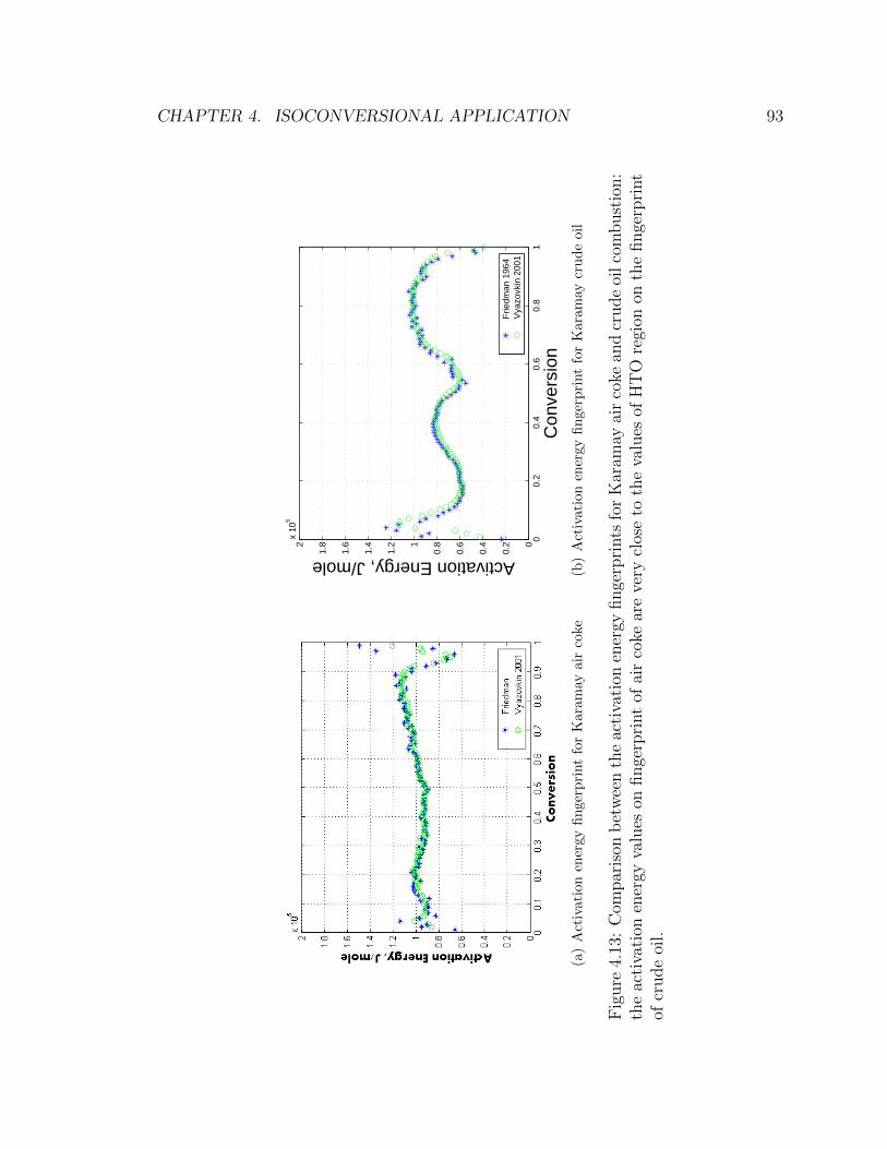
CHAPTER 4. ISOCONVERSIONAL APPLICATION 93
(a)
Act
ivat
ion
ener
gyfi
nge
rpri
nt
for
Kara
may
air
coke
00.
20.
40.
60.
81
0
0.2
0.4
0.6
0.81
1.2
1.4
1.6
1.82
x 10
5
Con
vers
ion
Activation Energy, J/mole
Frie
dman
196
4V
yazo
vkin
200
1
(b)
Act
ivati
on
ener
gy
fin
ger
pri
nt
for
Kara
may
cru
de
oil
Fig
ure
4.13
:C
ompar
ison
bet
wee
nth
eac
tiva
tion
ener
gyfinge
rpri
nts
for
Kar
amay
air
coke
and
crude
oilco
mbust
ion:
the
acti
vati
onen
ergy
valu
eson
finge
rpri
nt
ofai
rco
kear
eve
rycl
ose
toth
eva
lues
ofH
TO
regi
onon
the
finge
rpri
nt
ofcr
ude
oil.

CHAPTER 4. ISOCONVERSIONAL APPLICATION 94
4.2.2 Coke formed under nitrogen
Pyrolysis reactions happen where oxygen concentration is very low and temperature is
high enough to break molecular bonds of hydrocarbons, releasing light hydrocarbons
such as methane. During an ISC process, pyrolysis takes place in three stages: ignition
where nitrogen is injected and a heat is applied; coke zone in front of the combustion
zone where oxygen is not able to penetrate the combustion front, only nitrogen and
carbon oxides are present; the medium temperature reaction stage in between the
LTO and HTO [8][21]. One of the products of the pyrolysis reaction is coke. It
is regarded as the critical reactant during the ignition period and temperature front
propagation. Hayashitani et. al. [38] proposed a reaction scheme for thermal cracking
of crude oil, that is composed of three reactions and four components, asphaltenes,
maltenes, coke and distillates (Reaction scheme 4.2).
Asphaltenesk1−→ Coke (4.2a)
Maltenesk2−→ Asphaltenes (4.2b)
Maltenesk3−→ Distillates (4.2c)
Injection of N2 gas to obtain inert conditions is done to generate pyrolysis coke
(N2 coke) in the isothermal experiments. The same procedure is conducted as that
used for air coke investigation. The first is to define the termination temperature
through an RTO test shown in Figure 4.14. The temperature of 420 ◦C is selected as
methane is produced by pyrolysis reactions. The sample mixture of 45 gram is put
into the isothermal kinetic cell, pressure is fixed at 100 psi, and a N2 injection rate
of 2 L/min is applied. Four isothermal experiments are carried out and the heavy
residues within the porous media are removed by toluene.
RTO experiments are conducted to investigate the reaction kinetics of N2 coke.
Each experiment uses a coke mixture of 30 grams, and totally four RTO experiments
are conducted, of which the temperature and effluent gas histories are shown in Figure
4.15. N2 coke combustion represent a slight difference in oxygen consumption histories

CHAPTER 4. ISOCONVERSIONAL APPLICATION 95
Figure 4.14: Defining the termination temperature for the isothermal experiment ofN2 coke formation: 420 ◦C is selected.
when compared to that of the air coke. Two oxygen consumption humps are observed
and they are very close to each other. The isoconversional fingerprint on Figure 4.16
shows two reaction stages corresponding to the two oxygen humps. The two reaction
stages have activation energies around 0.8 × 10⁵ and 1.0 × 10⁵ J/mole. Comparing
with the activation energy of air coke, which is around 1.0 × 10⁵ J/mole, these two
kinds of different coke represents very similar kinetic character. This is also a good
news for ISC modeling that when building a reaction model for burning, we do not
really need to separate coke formed in different conditions, such as LTO and pyrolysis.
Similar conclusion can be seen in research of Belgrave et al. [6].
4.2.3 XPS analysis
The basic theory of the XPS technique is to estimate the binding energies of the
element. The solid sample is mounted on a stage within a vacuum. Monochromatic
X-Rays bombard the sample, causing electrons to be released from the sample sur-
face. The electron energy is counted and binding energies are estimated to produce

CHAPTER 4. ISOCONVERSIONAL APPLICATION 96
0 50 100 150 200 250 300 350 400200
300
400
500
600
700
800
900
1000
Time,min
Tem
pera
ture
, K
3.00 K/min
2.42 K/min
2.09 K/min
1.74 K/min
(a) Temperature histories
0 50 100 150 200 250 300 350 4000
0.05
0.1
0.15
0.2
0.25
0.3
0.35
0.4
Time,min
O2 c
onsu
mpt
ion,
Mol
e fr
actio
n
3.00 K/min2.42 K/min2.09 K/min1.74 K/min
(b) Oxygen consumption histories
Figure 4.15: RTO experiments for the Karamay N2 coke

CHAPTER 4. ISOCONVERSIONAL APPLICATION 97
0 0.2 0.4 0.6 0.8 10
0.2
0.4
0.6
0.8
1
1.2
1.4
1.6
1.8
2x 10
5
Conversion
Act
ivat
ion
Ene
rgy,
J/m
ole
Friedman 1964Vyazovkin 2001
Figure 4.16: Activation energy fingerprint for Karamay N2 coke
a spectrum of electron intensity as a function of electron energy [11][17]. Using XPS
analysis, chemical elements and functional groups on the sample surface are deter-
mined.
XPS analysis is used to investigate the difference between coke formed under air
and nitrogen conditions. Four spots are chosen for each coke sample. XPS survey
spectra for the air coke and the nitrogen coke is shown in Figures 4.17 and 4.18
respectively. Elements of oxygen and carbon on the coke surface are identified from
the survey. The ratios of oxygen and carbon are listed in Table 4.4. The oxygen
compositions are detected on the coke formed under nitrogen condition. The oxygen
may come from the crude-oil or from some residual air within the vacuum. Therefore,
it is not the existence of oxygen on the coke surface that is interesting to us, but the
oxygen carbon ratios. According to Table 4.4, the coke formed under the air flow
condition has greater oxygen-carbon ratios across the sample than the coke formed
under nitrogen condition. This suggests that the coke formed in the LTO reactions
has oxygen bonding on the surface.
High resolution XPS spectra of coke precipitated under the air and the nitrogen

CHAPTER 4. ISOCONVERSIONAL APPLICATION 98
flow conditions is shown in Figure 4.19. C-O functional group can be clearly seen on
the air coke sample, while only carbide is detected on the nitrogen coke sample.
Table 4.4: Oxygen carbon ratios on the surface of different coke under air and nitro-gen.
Coke under air (A) (B) (C) (D)Oxygen 40.84% 48.51% 39.64% 54.99%Carbon 47.36% 51.49% 60.36% 45.01%Ratio 0.86 0.94 0.66 1.22Coke under nitrogen (A) (B) (C) (D)Oxygen 40.65% 40.83% 39.28% 36.66%Carbon 59.35% 59.17% 60.72% 63.34%Ratio 0.68 0.69 0.65 0.58
4.3 ISC candidate screening
In-situ combustion has been successfully applied in many unconventional crude oil
fields since the first ISC pilot in the former Soviet Union in 1933-1934 and later a
field production in the USA in 1950-1951 [102][91]. Over the 80 years of research and
experiences on the field operation in ISC projects, a consensus has been reached that
screening of candidate fields is essential to reduce the failure risk of a commercial field
project. When evaluating the feasibility of this EOR technique in a certain crude-oil
reservoir candidate, reservoir geology, fluid properties and rock mineralogy need to
be analyzed due to their impact factors for the success of a field implementation.
Practically in the laboratory research, considerations of impact from rock and fluid
properties and the interaction between them are taken into account, while reservoir
geological impacts are neglected because of the limitation on generating heterogene-
ity or matrix fractures in the combustion tube scale. Monitoring ISC processes at
the field scale is very difficult, however, lab-scale combustion tube tests can mimic
the burning characteristics so that we can study ISC with effects of varying process
conditions. The combustion behavior primarily depends on its reaction kinetics. We

CHAPTER 4. ISOCONVERSIONAL APPLICATION 99
Figure 4.17: XPS survey spectra of coke formation under air flow condition. Fourspots are scanned.

CHAPTER 4. ISOCONVERSIONAL APPLICATION 100
Figure 4.18: XPS survey spectra of coke formation under nitrogen flow condition.Four spots are scanned.

CHAPTER 4. ISOCONVERSIONAL APPLICATION 101
Figure 4.19: High resolution XPS C 1s spectra of coke samples precipitated under airand nitrogen flow conditions

CHAPTER 4. ISOCONVERSIONAL APPLICATION 102
Figure 4.20: Unsuccessful combustion front propagation: (left) Combustion tubetemperature profile and (right) isoconversional fingerprint [17].
make the in-situ combustion kinetic characters as the criterion to screen the crude
oil candidate. As we know that the composition of the crude oil as well as the rock
property determines the fuel deposition during the ISC process, and this criterion is
well studied by analyzing the isoconversional fingerprint to make primary judgment
whether the candidate is good or not.
Previous research on basic screening for ISC candidates includes using TGA to
measure kinetic parameters of crude oil combustion. Verkoczy et al. [105] developed
screening criteria by processing the TGA results of eight primary and tertiary well-
head oil samples. Another attempt comes from study by Yannimaras et al. [119].
They built the screening criterion by applying a specially modified accelerating-rate
calorimeter (ARCTM) to gain reaction kinetic data for four crude oils of medium to
high gravity. By applying the isoconversional principle, Cinar et al. [18][17] studied
twelve crude-oil/sand-matrix pairs using RTO experiments with interpretation by the
isoconversional principle to get the activation energy fingerprint. Poor ISC candidates
represent very different isoconversional behavior from good candidates. On the fin-
gerprint, an activation energy barrier is detected at the early stage of the combustion
(Figure 4.20), while this energy barrier does not exist for the good candidate cases.
The isoconversional principle, as described in the previous chapter, processes tem-
perature and effluent gas data from RTO experiments. The non-isothermal condition

CHAPTER 4. ISOCONVERSIONAL APPLICATION 103
allows wider temperature measurement and thus the activation energy fingerprint
represents the performance of the whole progress of the combustion. Also, as dis-
cussed before, the kinetic cell study well separates fluid flow dynamics from reaction
dynamics. The fingerprint represent the apparent activation energy accounting for
reaction paths influenced not only by component reaction itself, but also combines
information from interaction between crude oil and rock matrix as well as interfere
from phase equilibrium. So this fingerprint can be treated as a diagnostic tool to infer
good candidates for an ISC process.
Isoconversional fingerprints are available for three cases: Alaska crude oil with
60 mesh sand and clay, Alaska crude oil with 60 mesh sand, and Karamay crude oil
with the reservoir sand. As discussed in the Section 4.1, the three cases show typical
reaction paths and no activation energy barrier is observed from the isoconversional
fingerprints. The combustion tube tests for the three cases are run in the dry forward
combustion mode. A heater is located near the top end of tube and thermocouples
along the combustion tube record the position of temperature front.
The combustion tube results are shown in Figure 4.21, 4.22 and 4.23 respectively.
When clay is mixed into the Alaskan crude oil sample (Figure 4.21), the combustion
is more intensive with an average combustion front peak temperature of 560 ◦C, and
CO2/CO of 3.25. Without the clay addition (Figure 4.22), the combustion has lower
front peak temperature which is 530 ◦C, and CO2/CO of 2.4. For the Karamay
crude oil with reservoir sand case in Figure 4.23, the peak front temperature is about
550 ◦C and CO2/CO is 6.3. The Karamay reservoir sand has clay in the mixture
which enhances the combustion regarding the high propogation temperatures and the
CO2/CO ratio.

CHAPTER 4. ISOCONVERSIONAL APPLICATION 104
10 20 30 40 50 60 70 80 90 100
100
200
300
400
500
600
700
Distance, cm
Tem
pera
ture
, C
44.3 min124.2 min132.9 min146.8 min156.1 min168.4 min202.2 min211.6 min228.0 min262.5 min269.5 min290.6 min314.4 min343.5 min361.8 min
(a) Temperature propagation
0 50 100 150 200 250 300 3500
2
4
6
8
10
12
14
16
18
Time, min
Gas
com
post
ion,
Mol
ar %
O2COCO2CH4
(b) Effluent gas histories
Figure 4.21: Alaska crude oil combustion tube test with 60 mesh sand and clay.

CHAPTER 4. ISOCONVERSIONAL APPLICATION 105
10 20 30 40 50 60 70 80 90 100
50
100
150
200
250
300
350
400
450
500
550
600
Distance, cm
Tem
pera
ture
, C
57 min104 min117 min130 min147 min160 min191 min208 min224 min258 min275 min296 min310 min346 min361 min
(a) Temperature propagation
0 50 100 150 200 250 300 3500
2
4
6
8
10
12
14
16
18
Time, min
Gas
com
post
ion,
Mol
ar %
O2COCO2CH4
(b) Effluent gas histories
Figure 4.22: Alaska crude oil combustion tube test with 60 mesh sand.

CHAPTER 4. ISOCONVERSIONAL APPLICATION 106
10 20 30 40 50 60 70 80 90 100
50
100
150
200
250
300
350
400
450
500
550
600
Distance, cm
Tem
pera
ture
, C
90 min142.3 min154.9 min175.7 min196.3 min228.2 min262.6 min284.4 min308.2 min348.1 min387.0 min436.5 min465.3 min477.6 min
(a) Temperature propagation
0 50 100 150 200 250 300 350 400 4500
2
4
6
8
10
12
14
16
18
Time, min
Gas
com
post
ion,
Mol
ar %
O2COCO2CH4
(b) Effluent gas histories
Figure 4.23: Karamay crude oil combustion tube test with reservoir sand.

Chapter 5
RTO kinetics using
electromagnetic radiation
In-situ combustion is an effective thermal enhanced oil recovery (EOR) process that
provides an important alternative to other EOR methods. Combustion reaction ki-
netics research is fundamental and essential to understand the high temperature com-
bustion front propagation process within the reservoir so that the project operation is
well controlled and the production is predictable. Conventional experimental tools to
estimate kinetic parameters of crude-oil oxidation include accelerated rate calorime-
try (ARC) [119] and thermogravimetric analysis (TGA) [60]. The interpretation of
the measured data relies on the assumption of a reaction model, however, it may
oversimplify the physics of crude-oil combustion. The isoconversional principle is an
alternative to the conventional methods with its model-free character to estimate
activation energy by interpreting effluent gas and temperature data from ramped
temperature oxidation (RTO) experiments. Cinar et al. applied the isoconversional
method to the analysis of RTO kinetic data of different crude-oil combustion experi-
ments and reported great potential for deconvolving the parallel and series reactions
characterizing ISC and screening potential candidates [14][15][16][17].
As discussed in the previous chapters, the isoconversional principle is applied to
post-process temperature and effluent gas data from a series of RTO experiments of
at least two heating rates. When considering the issue of data consistency, four or
107

CHAPTER 5. RTO KINETICS USING ELECTROMAGNETIC RADIATION 108
more RTO experiments are needed to characterize linearity as discussed in Chapter 2.
The RTO experiment within a kinetic cell system runs at a relatively low heat rate in
order to reduce the temperature deviations as well as to well separate reaction stages.
According to our former experiments, a heat rate less than 3 K/min is suggested.
Considering a termination temperature of 650 ◦C, it may take four to seven hours to
finish an experiment. Currently, the kinetic cell in the combustion lab is heated up by
an electric furnace [17], that consists of a coil heater and thermal insulation paddings.
Normally, the system takes overnight to allow the furnace to cool down to the ambient
temperature before we can conduct new experiments. The efficient use of time is
very low when we carry out four or more experiments to get the activation energy
fingerprint. This motivates us to find an unconventional heating method in place of
the electric furnace to heat up the kinetic cell. The electromagnetic heating has great
potential to improve the kinetic cell system with respect to high efficiency in heating
and cooling, parallel manipulation to process several experiments simultaneously, and
a more compact system design.
Since the 1980’s when the use of microwave radiation to heat chemical reactions
began, thousands of publications have described this electromagnetic heating method
applied in a broad range of science and engineering research, including drug discovery
[56], analytical chemistry [66], organic synthesis [66], inorganic synthesis [66], food
chemistry [76], materials science [44], enhanced oil recovery [13] and upgrading of oil
shale [45]. Compared to conventional heating methods that depend highly on external
heaters and in which energy is delivered by conduction, convection, or radiation, the
benefits of microwave heating come from the direct coupling of an electromagnetic
field with the sample to be heated. Accordingly, the heating efficiency is greater, the
heating rate is faster, and homogeneous temperature distribution is obtained because
of the deep penetration of microwave radiation.
There are two main microwave heating mechanisms [57] that are schematically
plotted in Figure 5.1, dipolar polarization and ionic conduction. Both microwave
heating mechanisms produce heating through molecular friction and dielectric loss.
The dipole or ion field attempts to realign itself with the alternating electric field
at microwave frequencies thereby attenuating electromagnetic energy. The ability of

CHAPTER 5. RTO KINETICS USING ELECTROMAGNETIC RADIATION 109
Figure 5.1: Schematic diagram of microwave heating mechanisms: dipolar polariza-tion and ionic conduction [26].
a specific material to absorb microwave energy is determined by the so-called loss
tangent, tanδ [56][57]. Generally, high tanδ materials are used for good absorption
of microwave with the standard operating frequency, such as 2.45 GHz. Reaction
vessels used in microwave assisted experiments are usually made out of microwave
transparent materials such as glass or Teflon (tanδ < 0.01), so that only the reaction
mixture rather than the reaction vessel is heated [57][83]. Because of direct coupling
of microwaves with the sample, microwave heating presents a reverse temperature
gradient to conventional heating, and it has the highest temperature in the center of
samples. Both heating methods are demonstrated in Figure 5.2.
By applying RTO principles, combustion kinetics is studied in lab using a RTO
kinetics cell. Currently, the kinetics cell is heated by an electric furnace that has a rel-
atively large cavity and long heating and cooling cycles. The furnace is air cooled and
usually more than a day is needed to let the system fall back to the ambient tempera-
ture before a new experiment can be started. Meanwhile, because of the large furnace
size and the complicated system operation, it is hard to achieve parallel manipulation
so that five or more simultaneous experiments with different heat rates are carried
out for isoconversional interpretation. Introducing the microwave heating method to
our oxidation kinetic experiments is attractive and has great potential in improving

CHAPTER 5. RTO KINETICS USING ELECTROMAGNETIC RADIATION 110
Figure 5.2: Temperature distribution difference between conventional and microwaveheating [57].
data quality and quantity. Table 5.1 lists some typical aspects of microwave heating
and furnace heating. As seen from the comparison in Table 5.1, microwave heating
has advantages with respect to setup size, heating circle, and parallel experimental
conditions. However, it does have some disadvantages in temperature measurement,
system control, and setup cost. With the well developed microwave heating technolo-
gies nowadays, these disadvantages do not limit applications.
Before implementing microwave heating in our reaction kinetics experiments, we
Table 5.1: Comparison between microwave heating and furnace heating
Microwave (quantity) Furnace (quantity)
Instrument size Small Less than 2 L Big More than 10 LHeating circle Short About 1 hour Long More than 1 dayPrecise control Difficult – Easy –T measurement Difficult – Easy –Parallel manipulation Easy – Difficult –System cost High More than $20,000 Low About $1,200
CHAPTER 5. RTO KINETICS USING ELECTROMAGNETIC RADIATION 111
have to consider various aspects: non-thermal effects of microwave radiation kinetics,
temperature measurement in an electromagnetic environment, reactor design, heat
loss from the reactor wall to the environment, oxidation gas supply to the reactor,
effluent output and analysis, power control, and so on. These issues have been well
studied through literature review and preliminary experiments.
5.1 Literature review
5.1.1 Microwave heating effect
In a microwave heating process, microwave interacts with a dielectric media and the
electromagnetic energy is converted into heat inside the sample. This is in contrast
to conventional heating where heat transfers from the sample surface towards the
center mainly by heat conduction. In general, the temperature inside the sample
within a conventional furnace is lower than that at the surface because heat has to
be transported from the surface to the interior. In the case of microwave heating, the
radiation energy is dissipated within the sample more or less uniformly and a much
greater heating rate is obtained. As a result, a significant temperature gradient can
also exist but with the inside hotter than the surface [123].
The average power, Pabs, dissipated in a dielectric of volume V is related to the
electric field E and the material dielectric properties by Eq. 5.1 [69]:
Pabs = 2πfε0ε′′
effE2rmsV (5.1)
where f is the frequency of the radiation, ε0 is the permittivity of free space, and ε′′
eff
is the complex component of the relative permittivity of the dielectric, also known as
the effective relative dielectric loss factor, and Erms is the root mean square of the
electric field E. Eq. 5.1 represents the relation between the volumetric absorption of
microwave power and the electromagnetic field for a given dielectric. In microwave
heating, microwaves only penetrate a limited distance below the sample surface and
this is represented by the penetration depth Dp [69]:

CHAPTER 5. RTO KINETICS USING ELECTROMAGNETIC RADIATION 112
Dp =λ0
2π
√ε′
ε′′(5.2)
where λ0 is the wavelength of the microwave radiation,√ε′ is the dielectric constant
that describes the ability of a molecule to be polarized by the electric field, and ε′′
is the dielectric loss which measures the efficiency to convert the electromagnetic
radiation into heat.
It can be seen from both Eq. 5.1 and 5.2 that the amount of microwave power
absorbed by the dielectric is dependent on the electromagnetic field applied and on
the dielectric property of the material heated. In a simple way, the ratio of the
dielectric loss and the dielectric constant is commonly used to measure the ability of
a material to convert microwave radiation into heat energy at a given frequency and
temperature, and this is referred to as the loss tangent:
tanδ =
√ε′′
ε′(5.3)
This suggests that under the same microwave heating conditions, some materi-
als are more capable than others of absorbing microwave radiation because of their
greater dielectric loss property. Passive heating elements, for example silicon carbide
or graphite-doped Teflon, have big loss tangent and are widely applied to material
processing that requires very high heat rates and high temperature conditions [57].
The Arrhenius expression for rate constant in Eq. 2.4 claims the increased reaction
rate constant as temperature increases. The rapid heating experienced in microwave-
assisted transformations may lead to altered product distributions, for instance fewer
by-products are generated comparing to a conventional oil bath reflux experiment.
These observed rate-accelerations and altered product distributions of microwave re-
actions compared to traditional heating experiments have led to debates on the exis-
tence of so-called ”specific” or ”non-thermal” microwave effects [57]. Pillai et al. [82]
conducted comparison experiments between conventional and microwave heating hy-
drodechlorination reaction. An expeditious hydrodechlorination of chlorobenzenes is
observed over 0.5% Pd/Al2O3 catalyst by conducting the reaction under microwave
irradiation conditions. Djenni et al. [24] investigated microwave selective heating

CHAPTER 5. RTO KINETICS USING ELECTROMAGNETIC RADIATION 113
phenomena and their impact on heterogeneous chemical reactions. They discussed
the non-thermal effect of microwaves and claimed that direct molecular activation
of microwaves should be excluded, because the energy used to ionize biological com-
pounds (13.6 eV ) is much higher than microwave energy (1.24×10⁻⁶ - 1.24×10⁻³ eV ).
They also developed a model to predict reaction kinetics and yields under microwave
heating based on the Arrhenius equation, and the model was in good agreement with
experimental data and procedures. In the majority of published cases, the reasons
for the observed rate enhancements and altered product distributions can probably
be attributed to the high reaction temperatures that can rapidly be attained when
processing heating in a microwave field. Silverwood et al. [95] compared experiments
of conventional and microwave heating for the oxidation of carbon monoxide over a
6.3% Pt/SiO2 catalyst (EUROPT-1). The microwave source used was a 2.45 GHz
generator up to 1 kW . The results showed both heating methods displayed similar
activities.
5.1.2 Temperature measurement
Temperature measurement inside a microwave cavity is very different as compared
to that in conventional heating systems, such as isomantles, oil baths, and hot
plates/wires [57]. In a microwave environment, temperature sensors are specially
designed to avoid influence or damage by electromagnetic waves. Temperature mea-
surement techniques can be classified into contact and non-contact modes. Ther-
mocouples, resistance temperature detectors (RTDs), and thermistors are the most
prevalent and low cost contact sensors. Fiber optic probes are accurate, but expensive
temperature measuring units. An infrared thermometer, which is a non-contact sen-
sor, measures infrared energy emitted by the materials. It is usually faster than the
contact sensors. Besides in place temperature determination, infrared thermal imag-
ing cameras are useful to capture temperature distribution on the sample surface
[80].
During the first years of microwave assisted heating research, temperature mea-
surement was often neglected for lack of suitable means [42]. The experimental results

CHAPTER 5. RTO KINETICS USING ELECTROMAGNETIC RADIATION 114
were compared with data in publications. Such comparison leads to incorrect esti-
mation of the capability of microwave radiation because of the significant difference
in temperature distribution between conventional heating and microwave heating as
found in later research.
A thermocouple is a thermoelectric temperature sensor consisting of two dissim-
ilar metallic wires coupled at the probe tip (measurement junction) and extended
to the reference (known temperature) junction. The temperature difference between
the probe tip and the reference junction is detected by measuring the change in volt-
age at the reference junction. Commercially available thermocouples have a metallic
body enclosing the sensor wires as insulation and protection. Using a thermocouple
to measure temperature within a microwave cavity when the magnetron is on causes
electrical arcing that damages the thermocouple. So early researchers turned off
the magnetron and then inserted a thermocouple to measure temperature. The mag-
netron was then restarted and the procedure repeated. Artificial error was introduced
by this approach that was corrected by some adjustments. For example, Perry et al.
[80] used a normal thermocouple to gain temperature values by inserting it through
a thin quartz tube into the heating sample patch bed after the microwave power was
turned off. Because of the error introduced by turning off the energy source, the tem-
perature decay curve was recorded on a strip chart recorder, and temperature versus
time curve was linearized by taking the natural log of the data and extrapolated to
zero time to determine operating bed temperature
A thermocouple encased in an electromagnetic sheath is currently the least expen-
sive method for temperature measurement in a microwave condition. The thermocou-
ple inside the sheath must be of the ungrounded tip variety, while grounding of the
metallic sheath to the cavity is required to avoid arcing. Shielding the thermocouple
circuit from the high voltage present in the microwave circuit required considerable
effort. It was possible to reduce interference to within the thermocouple resolution
(±1.5 ◦C). General guidelines in this regard are to use shielded extension cables
that should be grounded to the thermocouple amplifier circuitry and to remove such
circuitry as far as possible from the high voltage area. The amplifier circuitry also
needs to be designed to exclude electromagnetic interference from the high voltage

CHAPTER 5. RTO KINETICS USING ELECTROMAGNETIC RADIATION 115
circuit [9]. It is reported that a type S shielded thermocouple with platinum foil and
inert gas inlet can measure temperature up to 1700 ◦C in microwave sintering ceramic
process [29]. Furthermore, because shielded thermocouples have significant volume
due to the shielding, reaction volume should have a minimum size of approximately
30 ml [74]. Ripley [87] reported a patent on a very simple shielded thermocouple
and its embodiments. The thermocouple shield includes an electrically conductive
tube that protects the standard thermocouple from damage by microwave field and
a ceramic sheath in between the thermocouple and the conductive tube serves as
electrical insulation.
Fiber optic sensors are currently widespread but they are a relatively costly
method for temperature measurement. With this method, a fiber optic sensor with
gallium arsenide crystal on the tip is placed inside a protective tube directly into the
reaction mixture. One disadvantage compared to other measurement systems is the
more narrow operating range, usually of 0 to 300 ◦C Also they are very sensitive to
mechanical stress. Zhang et al. used a fiber optic sensor which had its tip at the
center of the catalyst sample to monitor the temperature in the microwave condition.
It is reported that sensor could in-situ measure temperature up to 1000 ◦C [121].
Infrared (IR) sensor is another widespread method which is noncontact and is
usually used to measure surface temperature. The sensors are integrated into the
wall of the microwave cavity and measurements are made from a certain distance.
The disadvantage of this method is that only the temperature of the outside wall of
the reactor is measured. In some experiments, sample surface temperature and center
temperature are gained simultaneously with IR sensor and a thermocouple or fiber
optic sensor, respectively, for comparison or feed back power controlling purposes [64].
5.1.3 Microwave heating system
Besides temperature measurement, a whole microwave heating system usually consists
of a reactor, which is a key component in microwave assisted research, microwave
generator, such as a magnetron, power tuning to adjust the heating rate, reaction
processing visualizing and wave guiding techniques to conduct an easily manipulated

CHAPTER 5. RTO KINETICS USING ELECTROMAGNETIC RADIATION 116
Figure 5.3: Temperature (T), pressure (p), and power (P) profile for a 3 mL sampleof methanol heated under sealed vessel single-mode microwave irradiation conditionsto 165◦C (external infrared temperature monitoring) [57].
experiment.
Early pioneering experiments based on microwave assistance have been carried out
in domestic microwave ovens. Since 2001, specifically designed dedicated microwave
reactors have been increasingly employed. These instruments feature built-in mag-
netic stirrers, direct temperature control of the reaction mixture with the aid of
internal fiber-optic probes or external infrared sensors, and software that enables on-
line temperature/pressure control by regulation of microwave power output. Since
the introduction of dedicated microwave reactors suitable for sealed vessel processing
in the year 2000, more than 2500 publications have described the used of such equip-
ment for carrying out a large variety of microwave assisted research [63] [3]. A variety
of microwave reactors and processing options are available today, and more than
90% of all currently published microwave protocols involving dedicated instruments
that rely on the use of so-called single-mode microwave reactors in combination with
sealed vessel processing. The temperature, power, and pressure profiles for a sample
of microwave-heated methanol shown in Figure 5.3 illustrate the operating principles
of a modern dedicated microwave reactor run in temperature control mode [57].

CHAPTER 5. RTO KINETICS USING ELECTROMAGNETIC RADIATION 117
5.2 Development of microwave heating systems
This section exhibits the development of three generations of microwave heating sys-
tem in the combustion lab. Preliminary tests on the systems as well as problems
are discussed. Meanwhile the proposal manipulations for parallel experiments are
included.
5.2.1 1st generation reactor and embodiments
The 1st generation microwave heating system is the first attempt to build up a pro-
totype. A household microwave oven of 700 W output power and 10 levels of power
control is used. The kinetic cell is made of a specially designed quartz tube that has
a large lip at the open end to aid the formation of a pressure-tight seal. The quartz
cell can stand temperatures of 1800 ◦C. A well machined metallic cap is used to seal
the open end of the tube and to hold the reactor in the center of the oven cavity. A
thermocouple is inserted through the metallic cap into the center of the quartz tube
to measure the in-situ reaction temperature. Another two holes on the top of the cap
serve as air injection and effluent conducting parts. This preliminary experimental
system is demonstrated in Figures 5.4 and 5.5.
Initially, we believed that microwaves from the magnetron would couple efficiently
with the crude-oil sample inside the quartz tube. In actual fact, there is no heat source
around the tube, as temperature increases, heat losses become larger and larger and
steady state may be achieved before our expected maximum temperature. Insulation
is used to reduce the heat loss from the tube to the cavity. Thermolastic insulation
is used and its properties are described by Marques et al. [67]. Figure 5.6 show the
insulation material and its embodiment around the quartz tube reactor.
Some basic tests showed that the dielectric properties of typical crude oils were
not sufficient to reach high temperature. In the best case, crude oils can only be
heated to 480 ◦C. Our experiments need to achieve a termination temperature up to
700 ◦C. The loss tangent of sintered SiC is 0.6 to 0.7 [61], and SiC is classified as a
high microwave energy absorber. Small cylinders of sintered SiC are added directly
to the sample to assist the absorption of microwave. The cylinders have a dimension

CHAPTER 5. RTO KINETICS USING ELECTROMAGNETIC RADIATION 118
Figure 5.4: Prototype of the 1st generation microwave heating system. The quartztube reactor is hung inside the microwave oven cavity.
Figure 5.5: Metallic cap on the top of the microwave oven. A thermocouple is in-serted through the cap. There are two connectors for injection and production gasrespectively. The cap needs to be well grounded.

CHAPTER 5. RTO KINETICS USING ELECTROMAGNETIC RADIATION 119
Figure 5.6: Insulation material and its embodiment around the quartz tube reactor:during an experiment, crude oil sample is put at the bottom of the quartz cell. Thebody of the tube is wrapped by insulation material that is transparent to microwave,reducing heat loss to the oven cavity.
Figure 5.7: Shielded thermocouple and sintered SiC cylinders: sintered SiC cylindersare mixed with crude oil sample, acting as energy absorber to assist fast heating.

CHAPTER 5. RTO KINETICS USING ELECTROMAGNETIC RADIATION 120
Figure 5.8: Schematic diagram of grounded circuit of a shield thermocouple.
of 5 mm in diameter and 10 mm in length. The number of SiC cylinders is varied
according to the desired heating rate of the experiments (Figure 5.7).
Temperature measurement is a critical issue as described in the literature review.
Fiber optic sensors have been widely used in microwave heating experiments. They
are costly, and especially for measurement up to 800 ◦C. A shielded metallic ther-
mocouple is used and it has worked very well for our experimental conditions. The
sheath consists of a stainless steel tube that blocks the direct coupling of microwave
with the metallic tip of the thermocouple. A ceramic tube is assembled in between
the thermocouple and the stainless steel tube and it plays the role as electric insu-
lation to avoid electrical arcing. Because of the metallic body of the thermocouple
as well as the sheath, a thermocouple and the stainless steel protection function as
a microwave antenna to conduct microwaves out of the cavity and cause hazards.
The bodies of the thermocouple and the protection tube are well grounded to the
interior wall of the microwave cavity. Microwaves are conducted back to the cavity
rather than transported outwards. The simple assembly of the thermocouple and its
embodiment in a microwave oven are displayed in Figure 5.7 and 5.8, respectively.
Two preliminary experiments were carried out to test the 1st generation system
and provide proof of concept. The test includes sealing the open end of the quartz
tube at elevated pressure up to 40 psi, measuring temperature with the shielded ther-
mocouple, injecting air, analyzing effluent gas with a gas analyzer, changing heating
rate with the various numbers of cylinders of sintered SiC, and presetting induced

CHAPTER 5. RTO KINETICS USING ELECTROMAGNETIC RADIATION 121
Table 5.2: Experimental conditions
Microwave (quantity) Furnace (quantity)
Experiment 1 40 6 40% 500 AirExperiment 2 14.5 3 1 30% 2500 N/A
power of the microwave oven. The experimental conditions are listed in Table 5.2.
Effluent gas results and temperature histories of the first experiment are shown in
Figure 5.9 and 5.10 respectively. From experiment 1, we find that when the temper-
ature reached about 400 ◦C, crude-oil cracking happened in which molecular bonds
are broken directly because of the heat. Methane was produced as a result [1]. With
temperature increasing, CO and CO2 fractions increase because of the termination
reactions (i.e. bond scission). When the temperature is above 600 ◦C, the reaction
stops because of the entire consumption of the crude oil within the quartz reactor.
This experiment used six pieces of SiC cylinders as the heating element mixed with
the crude-oil sample and set the power level as 40% of the full power. We achieved a
temperature as high as 600 ◦C in about 500 seconds.
The second experiment is conducted to test the variability of heating rate by
changing the number of SiC cylinders and the power level of the microwave oven.
Three SiC cylinders are added to the crude oil sample and 30% of the power level
is preset. We expect a lower heating rate in this experiment and the result shows a
maximum temperature of 600 ◦C achieved in about 2500 seconds.
Also, some comments are in order about the power control of the microwave oven.
When the oven is running at full power, the magnetron is working continuously. Once
the power is set to be a certain level below 100%, the magnetron runs in an on/off
mode in which the time portion is defined by the desired power level. So we can
expect a stair-step shape of the temperature profiles versus time.
5.2.2 2nd generation reactor and embodiments
The 2nd generation reactor is designed to overcome some limitations of the 1st gen-
eration reactor. The schematic design of the new reactor is shown in Figure 5.12.

CHAPTER 5. RTO KINETICS USING ELECTROMAGNETIC RADIATION 122
Figure 5.9: Experiment 1: effluent gas histories, 1st generation system.
Figure 5.10: Experiment 1: temperature profile, 1st generation system.

CHAPTER 5. RTO KINETICS USING ELECTROMAGNETIC RADIATION 123
Figure 5.11: Experiment 2: temperature profile, 1st generation system.
The thermocouple is a shielded thermocouple whose sheath is grounded to the
inside wall of the microwave cavity through the metal cap. Also, a channel on the
top of the cap conducts effluent gas to the gas analyzer. The quartz tube is divided
into two parts, and the lower part is filled with sand that disperses the injected air
and the middle part that holds the crude-oil sample. The thermocouple is inserted
through the metal cap into the center of the sample. An annular encasement holding
sintered SiC particles is wrapped around the bore of the quartz reactor. It plays the
role of energy absorber to heat up crude oil samples and to preheat the feed gas. Air
is fed through the bottom fitting of the reactor and is stirred by the sand inside the
tube. The gas is preheated to the same temperature as that of sample before it has
reaction with the sample.
The reactor is easily adjustable for different embodiments. Figure 5.13 shows the
embodiment based on a household microwave oven. We control the heating rate by
controlling the built-in power tuner or the mass of SiC absorber.
A prototype of the 2nd generation reactor is built according to the design in Figure
5.12. The reactor is embodied into a household microwave oven. The reactor and the
system are shown in Figure 5.14 to 5.17. The main body of the reactor is a quartz
tube of 1 inch in diameter and 7 inches in length. Both open ends of the tube are
sealed by Swagelok fittings with Teflon ferrules. One end the gas injection tubing is

CHAPTER 5. RTO KINETICS USING ELECTROMAGNETIC RADIATION 124
connected, and the other end has a channel to insert a shielded thermocouple and a
connecter to the products filter (Figure 5.14). The bottom part of the tube is filled
with fine sand to disperse the injection gas. The crude oil sample is mixed with small
cylinders of sintered SiC and fills the middle part of the quartz tube. The whole
reactor is hung inside the cavity of a household microwave oven (Figure 5.15). The
injection tubing connected with the bottom fitting is well grounded to the interior
wall of the cavity. An insulating ceramic tube is inserted into the channel first and
then a normal thermocouple with an ungrounded tip. The ceramic tube protects the
thermocouple from being destroyed by electrical arcing (Figure 5.16). The microwave
heating system is connected with the air mass flow meter and the product filter
(Figure 5.17).

CHAPTER 5. RTO KINETICS USING ELECTROMAGNETIC RADIATION 125
Fig
ure
5.12
:Sch
emat
icdes
ign
ofth
e2n
dge
ner
atio
nre
acto
r.

CHAPTER 5. RTO KINETICS USING ELECTROMAGNETIC RADIATION 126
Figure 5.13: The reactor embodiment based on a microwave oven.
5.2.3 3rd generation reactor and embodiments
Based on our preliminary tests on the 2nd generation system, several drawbacks
are observed. The first is that it is hard to carry out experiments at high pressure
condition because of the quartz tube fittings. The quartz tube is very fragile, but we
need to fasten the fitting tightly enough to stand high pressure condition. Excessive
tightening breaks the quartz tube. The second drawback is to preheat the inlet gas.
In-order to heat up the gas at the same temperature as that in the oil sample, extra
equipment such as electrical coil or furnace and temperature feedback and controlling
system are needed, which will make the system larger and more complicated. The
third drawback is that it is very difficult to remove the quartz tube from the microwave
cavity because of the fittings at both ends of the quartz tube. If we want to take the
sample out of the cavity while the temperature is still high, it is impossible to do that
because sands will leak through the bottom of the tube.
We designed the 3rd generation system which we believe overcomes the shortcom-
ings of the 2nd generation system. The schematic design of the system is shown in
Figure 5.18. There are two tubes in the design. The outer tube is the sintered SiC
tube that absorbs microwave energy to generate high temperature, and the interior
tube is the quartz tube that is filled by sands at the bottom and oil sample in the

CHAPTER 5. RTO KINETICS USING ELECTROMAGNETIC RADIATION 127
Figure 5.14: The prototype of the 2nd generation microwave reactor.
Figure 5.15: The embodiment in a household microwave oven.

CHAPTER 5. RTO KINETICS USING ELECTROMAGNETIC RADIATION 128
Figure 5.16: Shielded thermocouple and product filter connecter.
Figure 5.17: 2nd generation microwave heating system.

CHAPTER 5. RTO KINETICS USING ELECTROMAGNETIC RADIATION 129
middle. Between the SiC and the quartz tube, there is room to circulate the inlet
gas like air or nitrogen. The sealing metallic cap consists of three pieces, the bottom,
and middle and the top pieces. There is a gas inlet connector on the middle piece.
The inlet gas is conducted through the connection, travels through the room between
the quartz tube and the SiC tube, and then passes the hole at the bottom of the
quartz tube to mix with the oil sample. In this way, the inlet gas is preheated by
the SiC tube before it is mixed with the sample. Meanwhile, the heat is brought
to the sample by conduction, convection and radiation, that keeps the temperature
difference between the oil sample and inlet gas as small as possible. On the top piece,
a thermal well that protects the thermocouple is placed. There is a connection to
conduct the effluent gas to the gas analyzer on this piece as well.

CHAPTER 5. RTO KINETICS USING ELECTROMAGNETIC RADIATION 130
Fig
ure
5.18
:Sch
emat
icdes
ign
ofth
e3r
dge
ner
atio
nre
acto
r.

CHAPTER 5. RTO KINETICS USING ELECTROMAGNETIC RADIATION 131
Figure 5.19: The prototype of the 3rd generation microwave reactor.
A prototype of the 3rd generation reactor is built according to the design in Fig.
5.19. The reactor is embodied into a household microwave oven. The reactor and the
system are shown in Fig. 5.20 and 5.21. The main body of the reactor consists of
a sintered SiC tube of 1.6 inches in diameter and 7.2 inches in length and a quartz
tube of 1 inch in diameter and 6.5 inches in length. On one end of the quartz tube,
there is a large lip for sealing and the other end of the tube is there a small hole of
0.1 inches in diameter for gas crossing. The whole reactor is hung inside the cavity
of a household microwave oven. The microwave heating system is connected with the
oxidation gas tank and the product filter (Figure 5.22).
The first experiment ran on the full power model of 700 W for about 15 minutes.
The quartz tube was filled by fine sands and air was injection by the rate of 1 L/min.
The pressure inside the kinetic cell is ambient. An insulating material, fiberglass [67],
was wrapped around the body of the sintered SiC tube to reduce heat losses to the
cavity. We see fast heat rate at the early stage and lower heat rate after 600 seconds
because of the heat lost. The maximum temperature was around 300 ◦C in this case.
The second experiment ran on the same conditions as the first one except for
the insulating material. Black aerogel [67] that has much better insulation effect
was used in this case. A higher maximum temperature of about 530 ◦C was gained
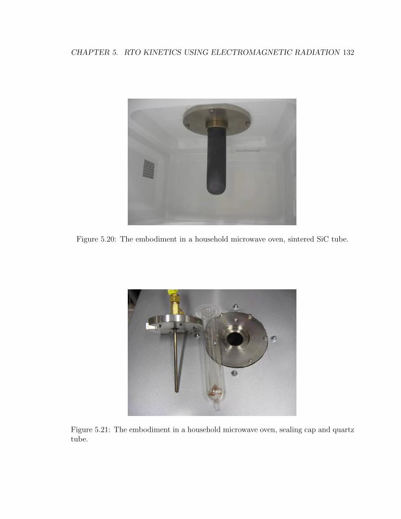
CHAPTER 5. RTO KINETICS USING ELECTROMAGNETIC RADIATION 132
Figure 5.20: The embodiment in a household microwave oven, sintered SiC tube.
Figure 5.21: The embodiment in a household microwave oven, sealing cap and quartztube.
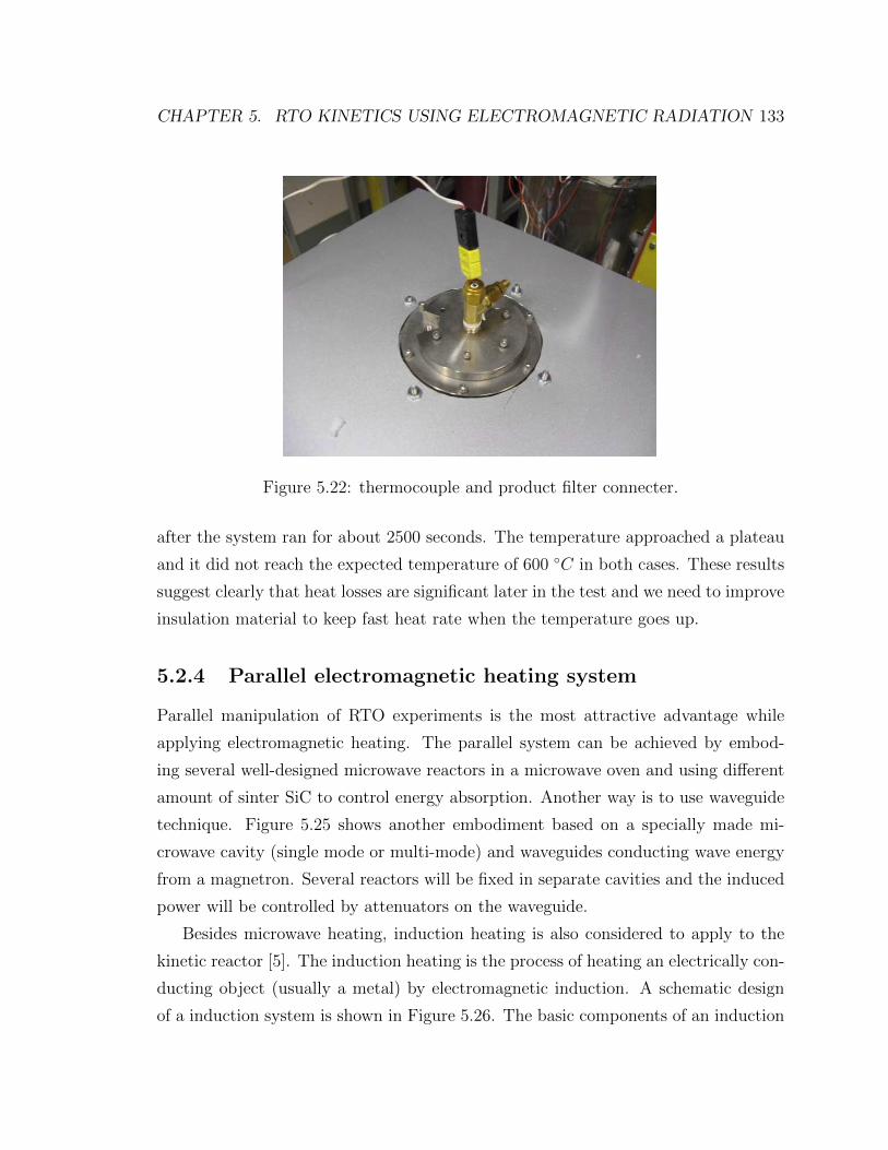
CHAPTER 5. RTO KINETICS USING ELECTROMAGNETIC RADIATION 133
Figure 5.22: thermocouple and product filter connecter.
after the system ran for about 2500 seconds. The temperature approached a plateau
and it did not reach the expected temperature of 600 ◦C in both cases. These results
suggest clearly that heat losses are significant later in the test and we need to improve
insulation material to keep fast heat rate when the temperature goes up.
5.2.4 Parallel electromagnetic heating system
Parallel manipulation of RTO experiments is the most attractive advantage while
applying electromagnetic heating. The parallel system can be achieved by embod-
ing several well-designed microwave reactors in a microwave oven and using different
amount of sinter SiC to control energy absorption. Another way is to use waveguide
technique. Figure 5.25 shows another embodiment based on a specially made mi-
crowave cavity (single mode or multi-mode) and waveguides conducting wave energy
from a magnetron. Several reactors will be fixed in separate cavities and the induced
power will be controlled by attenuators on the waveguide.
Besides microwave heating, induction heating is also considered to apply to the
kinetic reactor [5]. The induction heating is the process of heating an electrically con-
ducting object (usually a metal) by electromagnetic induction. A schematic design
of a induction system is shown in Figure 5.26. The basic components of an induction

CHAPTER 5. RTO KINETICS USING ELECTROMAGNETIC RADIATION 134
Figure 5.23: Temperature profile of microwave heating of test 1, 3rd generation sys-tem.
Figure 5.24: Temperature profile of microwave heating of test 2, 3rd generation sys-tem.

CHAPTER 5. RTO KINETICS USING ELECTROMAGNETIC RADIATION 135
Figure 5.25: Reactors based on microwave waveguides in a parallel manipulation.
heating system are an AC power supply, induction coil, and workpiece. The power
supply sends alternating current through the coil, generating a magnetic field. When
the workpiece is placed in the coil, the magnetic field induces eddy current in the
workpiece, generating precise amounts of clean, localized heat without any physi-
cal contact between the coil and the workpiece [88]. Parallel manipulation is easily
achieved in the induction heating method and the schematic designs are shown in
Figures 5.27 and 5.28. In Figure 5.27, eddy current strength is attenuated by voltage
transformer, while in Figure 5.28, different amounts of materials that attenuate elec-
tromagnetic radiation are mixed with samples in each reactor, and the reactors are
heated simultaneously in a semi-batch mode by the same electromagnetic radiation
source.
5.3 Discussion
Literature review has been done to show issues we have to figure out before building
a sophisticated electromagnetic heating system. Totally three generation microwave
heating systems have been built. Basic tests are conducted to show great poten-
tial of applying electromagnetic heating to carry out ramped temperature oxidation
experiments.

CHAPTER 5. RTO KINETICS USING ELECTROMAGNETIC RADIATION 136
Figure 5.26: Schematic of reactor heated by RF radiation.

CHAPTER 5. RTO KINETICS USING ELECTROMAGNETIC RADIATION 137
Figure 5.27: Induction heating with separate attenuator to achieve parallel heating.
Figure 5.28: Induction heating with different masses of RF absorber to achieve parallelheating.

CHAPTER 5. RTO KINETICS USING ELECTROMAGNETIC RADIATION 138
Future work is needed to reach reliably high temperatures. A better insulating
material may be needed to reduce the heat loss. Mixing small SiC cylinders with the
crude-oil sample is a good alternative to achieve high temperature as shown in the 1st
generation system, and improvement is needed to make the temperature distribution
more homogeneous during the heating period. Rather than using the built-in power
control system of the microwave oven, an well-designed power control system is needed
to control the temperature program more precisely.

Chapter 6
Summary and discussion
The combination of the ramped temperature oxidation (RTO) experiment and the
isoconversional principle interpretation unlocks the reaction kinetics of crude-oil com-
bustion in a practical fashion. The nonisothermal RTO experiments that undergo dif-
ferent heating rates widen the temperature range of data collection. This is believed
to be of great advantage over those experiments carried out under the isothermal con-
dition. The isoconversional principle is a model-free interpretation tool. The apparent
activation energy fingerprint represents the reaction paths. The two representative
reaction stages, LTO and HTO are easily identified. An ignition zone at the very
beginning and a transition zone in between LTO and HTO stages are also found.
The isoconversional fingerprint inherently contains impact factors on reaction paths
of the crude-oil combustion, such as reactions in different phases, interaction between
components, reservoir matrix surface area affect, and so on. Analyzing the fingerprint
provides significant information on the reaction kinetics of crude-oil combustion.
When applying the isoconversional principle to interpret effluent data from RTO
experiments, the very first and essentially important issue is the reliability of exper-
iments and data interpretations. This goes to the issue of consistency. Because of
the complicated reaction mechanism of the crude-oil combustion, minimizing heat
released from exothermic reactions is critical and necessary. This argument is sup-
ported by both simulations with a four-reaction synthetic model in a virtual kinetic
cell (VKC) simulator and experiments of different crude-oil sample mixtures. The
139

CHAPTER 6. SUMMARY AND DISCUSSION 140
heat released from reactions causes deviations on temperature profiles, that alter the
reaction paths and thus the isoconversional fingerprint. On the other hand, when the
heat released is controlled at a very low level, experiments of different injection gas
flow rates, different crude-oil sample sizes, and different kinetic cell designs exhibit
consistent isoconversional fingerprints. The results not only support the model-free
nature of the isoconversional principle, but also they convince us the combination
of RTO experiments and the isoconversional principle provide a reliable workflow to
investigate crude-oil combustion kinetics.
The activation energy values are the most critical parameter in building a reaction
model. The isoconversional principle is first developed to interpret activation energy,
however, its capability is far beyond the activation energy interpretation. Combin-
ing both the isoconversional principle and conventional interpretation methods de-
termines values for kinetic parameters, such as pre-exponential factor and reaction
orders. Rather than optimizing a multi-object function of the kinetic model (that
is always questioned by many researchers because of the mathematical solution lack
of physical meaning) interpreting parameter values from experimental measurements
using the combination method is more promising. A three-reaction scheme is pro-
posed based on the analysis of the isoconversional fingerprint and effluent data. Three
reaction stages are described in the scheme, including ignition, LTO and HTO stages.
Both simulations and experimental cases show the combination workflow to build a
reaction model for each reaction of the scheme. The simulation results for the com-
bustion of two crude-oil mixtures within a kinetic cell show good history matches
with respect to effluent gases and temperatures.
The isoconversional fingerprint represents the apparent reaction paths of the
crude-oil combustion. The reaction paths may have strong responses when the crude-
oil is mixed with rock matrix of different characters. The matrix surface area is a
critical factor for the heat conductivity during the combustion process, and thus the
reaction paths that are altered according to temperature variations. The surface area
effect, when analyzing the isoconversional fingerprint interpreted from RTO experi-
ments, is clearly observed. Smaller grain size implies greater surface area, and thus
more enhancement of crude-oil combustion. Coke formations under air and nitrogen

CHAPTER 6. SUMMARY AND DISCUSSION 141
conditions are investigated. The fuel for the HTO reaction is generated in a isother-
mal batch reactor at a certain temperature. The coke is extracted by toluene from
the fuel. Its characteristics are studied by RTO experiments and XPS analysis. The
isoconversional principle naturally deconvoles the multi-step reaction mechanism of
the crude-oil combustion. LTO and HTO reaction stages are easily identified from
the fingerprint. The isoconversional principle is applied to the RTO experiments to
interpret the activation energy fingerprint for coke. A good match of activation en-
ergy values between the coke and the HTO stage of the crude oil combustion is found.
XPS analysis of different kinds of coke formed under air and nitrogen conditions shows
more oxygen composition is found in the air coke than the nitrogen coke. Last but
not least is applying the isoconversional fingerprint as a diagnostic tool to screen the
crude-oil/matrix pairs as good candidates for the ISC process. The fingerprint of a
good candidate shows a smooth shape, while a bad candidate normally has an energy
barrier at the very beginning of the combustion process.
Applying the isoconversional interpretation to RTO experiments needs at least
four experiments at different heating rates. Because of the long heating-cooling cycle
of the electric furnace system, a faster and more compact kinetic cell system is more
preferred. Electromagnetic heating is a good candidate to replace the conventional
electric heating system. Not only the unconventional heating method makes the
system compact, achieving fast heating rates, shortening the heating-cooling circle,
but also the method can easily be expanded to parallel operation where several RTO
experiments are carried out simultaneously. Microwave are a kind of electromagnetic
energy. Three generations of the microwave heating system have been developed to
date. A maximum temperature of 500 ◦C is achieved.
The isoconversional principle is a useful interpretation tool to deconvolve the reac-
tion kinetics of crude-oil combustion. Future work is suggested to focus on applying
the principle to RTO experiments at large heating rates (> 20◦C/min). Because
of the complication of crude-oil reaction kinetics and the overlapped reaction zones,
faster heating rate experiments are expected to get lower apparent activation ener-
gies than that of experiments of low heating rates. Meanwhile more work is needed
to improve the proposed workflow of defining reaction parameters, such as reaction

CHAPTER 6. SUMMARY AND DISCUSSION 142
orders for fuel and oxygen partial pressure, and frequency factors. A more sophisti-
cated workflow is needed to post-process the RTO experiment data so that a robust
reaction model is built. The electromagnetic heating is believed to be great potential
to the RTO experiments. More work is needed to improve the system to achieve
high temperature, accurate temperature control and working under elevated pressure
conditions.

Appendix A
Updates for the kinetic cell and
combustion tube systems
1. Electric Furnace: Thermcraft No. XSL-3-0-18-1C is installed.
2. Solid state relay: No. SSR330DC25, 24 to 330 V AC, 25 Amp.
3. Temperature USB hub: 8 Channel Thermocouple Data Acquisition (DAQ)
Module.
4. Kinetic cell: the wall thickness is machined to be thinner than the previous
design. The adjustment is to make the temperature respond more quickly.
5. Isothermal kinetic cell: as described in Figure 4.9 in Chapter 4, the kinetic cell
is used to generate coke components at elevated pressure. It can be used as the
normal kinetic cell in RTO as well.
6. Gas analyzer: SERVOPRO 4200. The calibration gases for the gas analyzer is
O2 - 50%, CO2 - 25%, CO - 25%, N2 - 100%. The upper limit for measurement
of CO and CO2 is 25%.
7. Mass flow controller: it needs to be calibrated before experiments. Table A.1 is
for reference of air calibration.
143
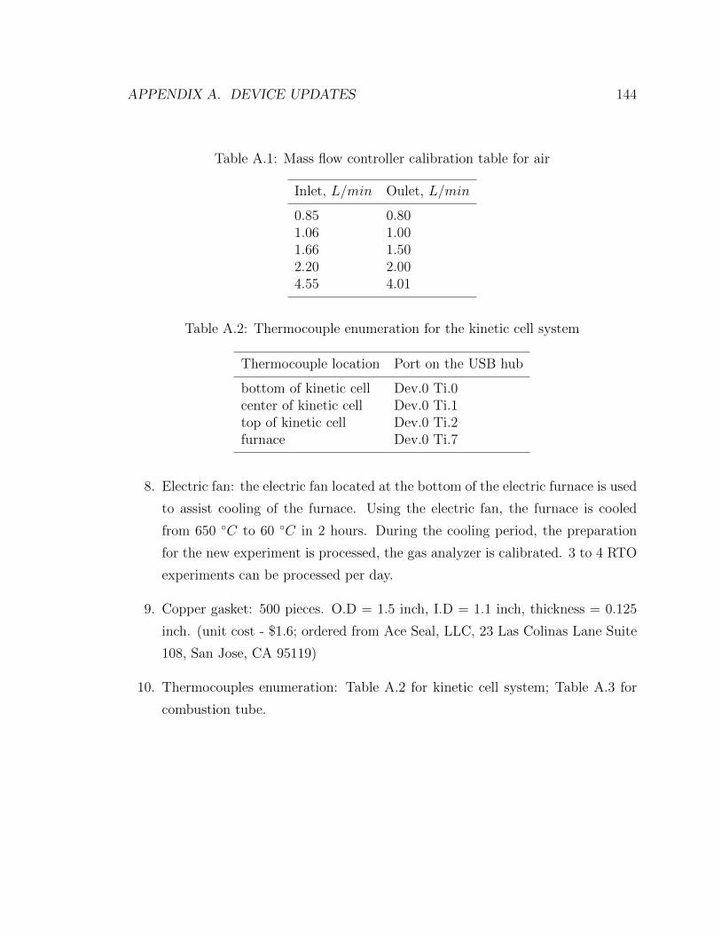
APPENDIX A. DEVICE UPDATES 144
Table A.1: Mass flow controller calibration table for air
Inlet, L/min Oulet, L/min
0.85 0.801.06 1.001.66 1.502.20 2.004.55 4.01
Table A.2: Thermocouple enumeration for the kinetic cell system
Thermocouple location Port on the USB hub
bottom of kinetic cell Dev.0 Ti.0center of kinetic cell Dev.0 Ti.1top of kinetic cell Dev.0 Ti.2furnace Dev.0 Ti.7
8. Electric fan: the electric fan located at the bottom of the electric furnace is used
to assist cooling of the furnace. Using the electric fan, the furnace is cooled
from 650 ◦C to 60 ◦C in 2 hours. During the cooling period, the preparation
for the new experiment is processed, the gas analyzer is calibrated. 3 to 4 RTO
experiments can be processed per day.
9. Copper gasket: 500 pieces. O.D = 1.5 inch, I.D = 1.1 inch, thickness = 0.125
inch. (unit cost - $1.6; ordered from Ace Seal, LLC, 23 Las Colinas Lane Suite
108, San Jose, CA 95119)
10. Thermocouples enumeration: Table A.2 for kinetic cell system; Table A.3 for
combustion tube.

APPENDIX A. DEVICE UPDATES 145
Table A.3: Thermocouple enumeration for the combustion tube
Thermocouple location Port on the USB hub
Heater Dev.1 Ti.0CH.1 Dev.1 Ti.1CH.2 Dev.1 Ti.2CH.3 Dev.1 Ti.3CH.4 Dev.1 Ti.5CH.5 Dev.1 Ti.6CH.6 Dev.1 Ti.7CH.7 Dev.2 Ti.0CH.8 Dev.2 Ti.2CH.9 Dev.2 Ti.3CH.10 Dev.2 Ti.4CH.11 Dev.2 Ti.5CH.12 Dev.2 Ti.7CH.13 Dev.3 Ti.0CH.14 Dev.3 Ti.2CH.15 Dev.3 Ti.3

Appendix B
Background correction of effluent
data
Effluent data drift causes the tail of the gas production history to be non-zero. It
makes the isoconversional interpretation inconsistent. The data drift is caused by
two factors: electric current of the gas module drifts in the gas analyzer, and some
components in the sand mixture are oxidized at high temperatures. The objective of
background correction of the effluent data is to force the non-zero values at the tail
of the gas production history to be zero.
The proposed method rotates the effluent data curve by a certain angle. The value
of the angle is determined by the first non-zero oxygen consumption point (i.e. where
the oxidation starts) and the expected completion point at the end of the oxidation.
Figure B.1 shows two similar temperature histories whose effluent data is expected
to be very similar as well. Because of the data drift, effluent data in Figure B.2(a) is
not consistent. After background correction by curve rotation, the result is shown in
Figure B.2(b), exhibiting very consistent behaviors.
% c u r v e s h i t .m
% r o t a t e e f f l u e n t curves to do back ground c o r r e c t i o n .
% Bo Chen , SUPRI−A, Stanford Un ive r s i ty
146

APPENDIX B. BACKGROUND CORRECTION OF EFFLUENT DATA 147
c l c ;
c l e a r a l l ;
end po int t ime = 18185 ; %second
load E:\matlabworks\Preproce s s ing \ input . txt ;
p l o t ( input ( : , 1 ) , input ( : , 2 ) ) ;
g r i d on ;
hold a l l ;
i ndex end po in t t ime = f i n d ( input ( : , 1 )==end po int t ime ) ;
p l o t ( input ( index end po int t ime , 1 ) , input ( index end po int t ime
, 2 ) , ’ r ∗ ’ ) ;
hold a l l ;
s h i t t a n a n g e l = input ( index end po int t ime , 2 ) / input (
index end po int t ime , 1 ) ;
f i r s t n o n z e r o = f i n d ( input ( : , 2 )>0) ;
f i r s t n o n z e r o = f i r s t n o n z e r o (1 ) ;
i n i t i a l p a r t = input ( 1 : f i r s t n o n z e r o −1 , : ) ;
end part = input ( index end po in t t ime +1:end , : ) ;
end part ( : , 2 ) = 0 ;
s h i t f p a r t = input ( f i r s t n o n z e r o : index end po int t ime , : ) ;
i f s h i t t a n a n g e l > 0
s h i t f p a r t ( : , 2 ) = s h i t f p a r t ( : , 2 ) − s h i t f p a r t ( : , 1 ) ∗s h i t t a n a n g e l ;
e l s e
s h i t f p a r t ( : , 2 ) = s h i t f p a r t ( : , 2 ) − s h i t f p a r t ( : , 1 ) ∗s h i t t a n a n g e l ;
end
s h i t f c u r v e = [ i n i t i a l p a r t ; s h i t f p a r t ; end part ] ;
p l o t ( s h i t f c u r v e ( : , 1 ) , s h i t f c u r v e ( : , 2 ) , ’ g ’ ) ;

APPENDIX B. BACKGROUND CORRECTION OF EFFLUENT DATA 148
hold o f f ;
l egend ( ’ o r i g i n a l ’ , ’ s h i f t e d ’ ) ;
Figure B.1: Temperature histories for RTO experiments.

APPENDIX B. BACKGROUND CORRECTION OF EFFLUENT DATA 149
(a) Before data background correction.
(b) After data background correction.
Figure B.2: Background correction example for two RTO experiments.

Appendix C
Kinetic cell experiment
preparation
Preparing the crude-oil sample mixture for consistent RTO experiments is critical.
Much care is needed. Some tips from my experience on preparing the sample mixture
are listed:
1. Sand is cooked for at least 4 hours at a temperature of 650 ◦C to oxidize reactive
components on the sand surface.
2. Use 25 g of the fired sand to fill up the dispersion cup at the bottom of the
kinetic cell.
3. A bigger sample mixture than the one used in the experiment is prepared. For
instance, while the Karamay crude-oil/sand mixture of 15 gram is used in the
RTO experiment, a bigger sample mixture of 25 gram is made. 15 gram is
taken from the bigger sample mixture and used in the experiment. This is just
to reduce errors caused by oil and water vaporization, oil residues on the mixing
spoons and cups, and imperfect mixing to make homogeneous sample mixture.
4. Two spoons are suggested when mixing the sample, so that the residual oil on
a spoon can be removed by the other one.
150

APPENDIX C. KINETIC CELL EXPERIMENT PREPARATION 151
5. After putting the crude-oil mixture in the center of the kinetic cell, the rest
room of the cell chamber is filled up with fired sand.
6. Fresh sample mixture is suggested for every RTO experiment, but it is not
necessary. The exposure of the mixture in the air causes water and light com-
ponents of the crude oil to be vaporized, but these components do not react
with oxygen during the RTO experiment.
7. Clean screws with lubricant everytime before assembling the kinetic cell. Wait
until the kinetic cell completely cooled down before unscrewing screws.

Appendix D
Codes for virtual kinetic cell
simulation and isoconversional
interpretation
The VKC and both differential and integral isoconversional methods are coded in
MATLAB. Funtions of the simulator are listed:
• ISCMainStart.m — input parameters and result plots;
• ActEnergy.m — differential and integral isoconversional methods;
• govenEqn.m — govening equations for the VKC;
• ISCsolver.m — equation solver;
• phiEnergy.m — sub-equation for the integral isoconversional method;
• prodRate.m — net reaction rate;
• prodRate2.m — net reaction rate;
• reactionRate.m — Arrhenius rate law;
152

APPENDIX D. VKC AND ISOCONVERSIONAL CODES 153
∗∗∗∗∗ ISCMainStart .m
% Vir tua l Kine t i c Ce l l S imulat ion
% ve r s i on 2 . 0 , updated on Apr i l 15 , 2011
% Developed by Bo Chen , SUPRI−A, Stanford Un ive r s i ty
% Tota l ly 7 s p e c i e s are in the r e a c t i o n scheme :
% A, C, and D are in l i q u i d / s o l i d phase ;
% Others are in gas phase ;
% Number o f r e a c t i o n s i s expandable through s t o i c h i o m e t r i
c o e f f i c i e n t matr i ce s
% r e a c t i o n mechanism
% A + B −> C, k1
% C −> D + F, k2
% A + B −> H + G + F, k3
% D + B −> H + G + F, k4
c l c ;
c l e a r a l l ;
MD. Arrhenius = [ 1 , 1 , 100 , 8 0 ; . . .
63000 , 80000 , 125000 , 1 0 0 0 0 0 ] ’ ; % constant
[ 1 / ( mole∗ s ) ] ; a c t i v a t i o n energy [ J/mole ]
MD. heatReact ion = [−10000 , 40000 , −60000 , −40000] ’ ; % heat o f
r e a c t i o n [ J/mole ]
MD.Cp = [ 2 0 0 . 0 , 35 , 100 , 100 , 50 , 60 , 3 5 ] ’ ; % heat capac i ty [
J/mole ]

APPENDIX D. VKC AND ISOCONVERSIONAL CODES 154
MD. n u j i p = [ 1 , 1 , 0 , 0 , 0 , 0 , 0 ; . . . // s t o i c h i o m e t r i
c o e f f i c i e n t matr i ce s
0 , 0 , 0 , 0 , 0 , 0 , 0 ; . . . // r eac tant
0 , 0 , 0 , 0 , 0 , 0 , 0 ; . . .
0 , 1 , 0 , 1 , 0 , 0 , 0 ] ;
MD. n u j i d p = [ 0 , 0 , 0 , 1 , 0 , 0 , 0 ; . . . // products
0 , 0 , 0 , 0 , 0 , 0 , 0 ; . . .
0 , 0 , 0 , 0 , 0 , 0 , 0 ; . . .
0 , 0 , 0 , 0 , 1 , 1 , 1 ] ; . . .
MD. r e a c t i o n o r d e r P = [ 1 , 1 , 0 , 0 , 0 , 0 , 0 ; . . . // r e a c t i o n
o rde r s
0 , 0 , 0 , 0 , 0 , 0 , 0 ; . . . // r eac tant
0 , 0 , 0 , 0 , 0 , 0 , 0 ; . . .
0 , 1 , 0 , 1 , 0 , 0 , 0 ] ;
MD. r eac t i on o rde r dP = [ 0 , 0 , 0 , 0 , 0 , 0 , 0 ; . . . // products
0 , 0 , 0 , 0 , 0 , 0 , 0 ; . . .
0 , 0 , 0 , 0 , 0 , 0 , 0 ; . . .
0 , 0 , 0 , 0 , 0 , 0 , 0 ] ; . . .
% I n i t i a l & Boundary cond i tons
IC . T0 = 2 9 8 . 1 5 ; % [K]
IC . Ua = 15000 ; % [ J /(mˆ3∗ s∗k ) ]
IC .V =0.00004; % [mˆ3 ]
IC . q = 2/(1000∗60) ; % volume frow ra t e
IC .P = 0.8∗100∗6 .894 e3 ; % p i s
R = 8 . 3 1 4 ;
IC . i n i t i a l C o n d = [20000 , IC .P/(R∗IC . T0) , 0 , 0 , 0 , 0 , 0 , IC . T0 ] ;
%rateHeat = [ 3 , 4 5 , 6 ] ’ / 6 0 ; % K/ sec
rateHeat = [ 1 . 5 4 , 1 . 7 4 , 1 . 9 3 , 3 . 3 ] ’ / 6 0 ; % K/ sec

APPENDIX D. VKC AND ISOCONVERSIONAL CODES 155
% Solve the govening equat ion
Tspan= [ 0 , 5 0 0∗ 6 0 ] ;
T int = 6000 ;
f o r i = 1 : l ength ( rateHeat )
IC . rateHeat = rateHeat ( i ) ; % K/ sec
[T, Y] = ISCso lver (MD, IC , Tspan ) ; % smal l numerica l
s o v l e r f o r k i n e t i c c e l l
t i m e l i n e ( : , i ) = l i n s p a c e (0 , Tspan (2 ) , T int ) ’ ;
comsuption B ( : , i ) = IC .P/(R∗IC . T0) − i n t e rp1 (T,Y( : , 2 ) ,
t i m e l i n e ( : , i ) ) ;
i ndex neg t i v e = f i n d ( comsuption B ( : , i )<0) ;
comsuption B ( index negt ive , i ) =0;
Temp line ( : , i ) = in t e rp1 (T,Y( : , end ) , t i m e l i n e ( : , i ) ) ;
end
f i g u r e
f o r i = 1 : l ength ( rateHeat )
p l o t ( t i m e l i n e ( : , i ) , comsuption B ( : , i ) , ’∗ ’ ) ;
hold a l l ;
end
x l a b e l ( ’ Temperature ’ ) ;
y l a b e l ( ’ Consumption ’ ) ;
e s t r a n g e = [−1e2 , 1 e6 ] ;
[ AEnergy1 , Conversion1 ] = ActEnergy ( comsuption B , Temp line ,
t i m e l i n e , ’ Friedman ’ , e s t r a n g e ) ;
%[AEnergy2 , Conversion2 ] = ActEnergy ( comsuption B , Temp line ,
t i m e l i n e , ’ Vyazovkin 1997 ’ , e s t r a n g e ) ;

APPENDIX D. VKC AND ISOCONVERSIONAL CODES 156
[ AEnergy3 , Conversion3 ] = ActEnergy ( comsuption B , Temp line ,
t i m e l i n e , ’ Vyazovkin 2001 ’ , e s t r a n g e ) ;
f i g u r e
%subplot ( 2 , 1 , 1 )
f o r i = 1 : l ength ( rateHeat )
p l o t ( t i m e l i n e ( : , i ) /60 , comsuption B ( : , i ) , ’∗− ’) ;
hold a l l ;
end
a x i s ( [ 0 , Tspan (2 ) /60 , 0 , 25 ] ) ;
g r i d on ;
x l a b e l ( ’ Time , min ’ , ’ FontSize ’ , 1 4 , ’ FontName ’ , ’ Aharoni ’ ) ;
y l a b e l ( ’O2 comsuption , mole/mˆ3 ’ , ’ FontSize ’ , 1 4 , ’ FontName ’ , ’
Aharoni ’ ) ;
l egend ( ’ 1 . 5 4 K/min ’ , ’ 1 . 7 4 K/min ’ , ’ 1 . 9 3 K/min ’ , ’ 2 . 6 4 K/min ’ ) ;
s e t ( legend , ’ FontSize ’ , 1 4 , ’ FontName ’ , ’ Aharoni ’ ) ;
hold o f f ;
f i g u r e
%subplot ( 2 , 1 , 2 )
f o r i = 1 : l ength ( rateHeat )
p l o t ( t i m e l i n e ( : , i ) /60 , Temp line ( : , i ) −273.15 , ’∗− ’) ;
hold a l l ;
end
g r id on ;
x l a b e l ( ’ Time , min ’ , ’ FontSize ’ , 1 4 , ’ FontName ’ , ’ Aharoni ’ ) ;
y l a b e l ( ’ Temperature , K’ , ’ FontSize ’ , 1 4 , ’ FontName ’ , ’ Aharoni ’ ) ;
l egend ( ’ 1 . 5 4 K/min ’ , ’ 1 . 7 4 K/min ’ , ’ 1 . 9 3 K/min ’ , ’ 2 . 6 4 K/min ’ ) ;
s e t ( legend , ’ FontSize ’ , 1 4 , ’ FontName ’ , ’ Aharoni ’ ) ;
hold o f f ;

APPENDIX D. VKC AND ISOCONVERSIONAL CODES 157
f i g u r e
%subplot ( 2 , 2 , 3 )
p l o t ( Conversion1 , AEnergy1 , ’ ∗ ’ , Conversion3 , AEnergy3 , ’ go ’ ) ;
a x i s ( [ 0 , 1 , 0 . 4 e5 , 1 . 4 e5 ] ) ;
g r i d on ;
x l a b e l ( ’ Conversion ’ , ’ FontSize ’ , 1 4 , ’ FontName ’ , ’ Aharoni ’ ) ;
y l a b e l ( ’ Act ivat ion Energy , J/mole ’ , ’ FontSize ’ , 1 4 , ’ FontName ’ , ’
Aharoni ’ ) ;
l egend ( ’ Friedman ’ , ’ Vyazovkin 2001 ’ , ’ Location ’ , ’ SouthEast ’ ) ;
s e t ( legend , ’ FontSize ’ , 1 4 , ’ FontName ’ , ’ Aharoni ’ ) ;
hold o f f ;
∗∗∗∗∗∗∗∗∗∗∗∗∗∗∗∗∗∗∗∗∗∗∗∗∗∗∗∗∗
∗∗∗∗∗∗ ActEnergy .m
func t i on [ AEnergy , Conversion ] = ActEnergy ( comsuption B ,
Temp line , t i m e l i n e , opt ions , e s t r a n g e )
% I s o c o n v e r t i o n a l method
% a c t i v a t i o n energy s o l v e r
R = 8 . 3 1 4 ;
num expij = s i z e ( comsuption B ) ;
num exp = num expij (2 ) ;
length B = num expij (1 ) ;
num interp = 100 ;
x= l i n s p a c e ( 0 . 0 0 1 , 0 . 9 9 9 , num interp ) ;
x = x ’ ;

APPENDIX D. VKC AND ISOCONVERSIONAL CODES 158
f o r i = 1 : num exp
index = f i n d ( comsuption B ( : , i ) >0.001) ;
i n d e x s t a r t = index (1 ) ;
index end = index ( end ) ;
Temp temp = Temp line ( i n d e x s t a r t : index end , i ) ;
Time temp = t i m e l i n e ( i n d e x s t a r t : index end , i ) ;
Time span temp = [ Time temp ( 2 : end ) ; 0 ] − Time temp ;
Time span = [ Time span temp ( 1 : end−1) ; Time span temp ( end
−1) ] ;
i s oconver t i onB = comsuption B ( i n d e x s t a r t : index end , i ) .∗Time span ;
B to ta l ( i ) = sum( i soconver t i onB ) ;
xx = ze ro s ( l ength ( i soconver t i onB ) ,1 ) ;
f o r j = 1 : l ength ( i soconver t i onB ) ;
xx ( j ) = sum( i soconver t i onB ( 1 : j ) ) / B to ta l ( i ) ;
end
Temp x ( : , i ) = in t e rp1 ( xx , Temp temp , x ) ;
x Time ( : , i ) = in t e rp1 ( xx , Time temp , x ) ;
end
i f strcmp ( opt ions , ’ Friedman ’ )
f o r i = 1 : num exp
dxdt ( : , i ) = in t e rp1 ( t i m e l i n e ( : , i ) , comsuption B ( : , i )
, x Time ( : , i ) , ’ s p l i n e ’ ) / B to ta l ( i ) ;
end
ln dxdt = log ( dxdt ) ;
f o r j = 1 : num interp
LineSlope = p o l y f i t (−1./(R∗Temp x( j , : ) ) , ln dxdt ( j , : ) , 1 ) ;
AEnergy ( j ) = LineSlope (1 ) ;
end

APPENDIX D. VKC AND ISOCONVERSIONAL CODES 159
AEnergy = AEnergy ’ ;
Conversion = x ;
end
% Vyazovkin
i f strcmp ( opt ions , ’ Vyazovkin 1997 ’)
d e l t a t = num interp ;
f o r index x = 2 : num interp
i f index x <= d e l t a t
Cal Ex ( index x −1) = fminbnd (@(Ex) phiEnergy ( Ex ,
Temp x ( 1 : index x , : ) , x Time ( 1 : index x , : ) ) ,
e s t r a n g e (1 ) , e s t r a n g e (2 ) ) ;
e l s e
Cal Ex ( index x −1) = fminbnd (@(Ex) phiEnergy ( Ex ,
Temp x( index x−d e l t a t +1: index x , : ) , x Time (
index x−d e l t a t +1: index x , : ) ) , e s t r a n g e (1 ) ,
e s t r a n g e (2 ) ) ;
end
end
AEnergy = Cal Ex ;
Conversion = x ( 2 : end ) ;
end
i f strcmp ( opt ions , ’ Vyazovkin 2001 ’)
d e l t a t = 2 ;
f o r index x = 2 : num interp
i f index x <= d e l t a t

APPENDIX D. VKC AND ISOCONVERSIONAL CODES 160
Cal Ex ( index x −1) = fminbnd (@(Ex) phiEnergy ( Ex ,
Temp x ( 1 : index x , : ) , x Time ( 1 : index x , : ) ) ,
e s t r a n g e (1 ) , e s t r a n g e (2 ) ) ;
e l s e
Cal Ex ( index x −1) = fminbnd (@(Ex) phiEnergy ( Ex ,
Temp x( index x−d e l t a t : index x , : ) , x Time ( index x−d e l t a t : index x , : ) ) , e s t r a n g e (1 ) , e s t r a n g e (2 ) ) ;
end
end
AEnergy = Cal Ex ;
Conversion = x ( 2 : end ) ;
end
∗∗∗∗∗∗∗∗∗∗∗∗∗∗∗∗∗∗∗∗∗∗∗∗∗∗∗∗∗∗∗∗
∗∗∗∗∗∗∗∗∗∗ govenEqn .m
func t i on dydt = govenEqn ( t , y ,MD, IC )
% y = [ x1 , x2 , x3 . . . xi ,T]
Arrhenius = MD. Arrhenius ;
heatReact ion = MD. heatReact ion ;
Cp = MD.Cp ;
n u j i p = MD. n u j i p ;
n u j i d p = MD. n u j i d p ;
r e a c t i o n o r d e r P = MD. r e a c t i o n o r d e r P ;
r ea c t i on o rde r dP = MD. r eac t i on o rde r dP ;
dim nu = s i z e (MD. n u j i p ) ;

APPENDIX D. VKC AND ISOCONVERSIONAL CODES 161
num spec = dim nu (2) ;
num reac = dim nu (1) ;
% I n i t i a l & Boundary cond i tons
T0 = IC . T0 ;
Ua = IC . Ua ;
V = IC .V;
q = IC . q ;
rateHeat = IC . rateHeat ;
R = 8 . 3 1 4 ; % J/mole . k
P = IC .P; % pa
index T = num spec + 1 ;
dydt = ze ro s ( index T , 1 ) ; % mole concent ra t i on and T
k f r = react ionRate ( num reac , Arrhenius , y ( index T ) ) ;
i f ( imag ( y (1 ) ) ˜= 0)
y (1 ) = 0 ;
end
i f y (1 ) < 0
y (1 ) = 0 ;
end
omega j = prodRate (MD, kfr , [ y (1 ) ; IC . i n i t i a l C o n d (2) ; y ( 3 :
end−1) ] ) ;
omega i = prodRate2 (MD, kfr , [ y (1 ) ; IC . i n i t i a l C o n d (2) ; y ( 3 :
end−1) ] ) ;
F B0 = P∗q /(R∗T0) ;
v r a t e = q ; % mˆ3/ s

APPENDIX D. VKC AND ISOCONVERSIONAL CODES 162
theta = ze ro s ( num spec , 1 ) ;
f o r j = 1 : num spec
theta ( j ) = ( y ( j )∗ v r a t e ) /F B0 ; %mole Fract ion
∗∗∗∗∗∗∗∗∗∗∗end
theta (1 ) = 0 ;
theta (3 ) = 0 ;
theta (4 ) = 0 ;
Ta = T0 + rateHeat ∗ t ;
Q = Ua∗V∗(Ta−y ( index T ) ) ;
% Govening eqaut ions
dydt (1 ) = omega j (1 ) ; % y i s mole concent ra t i on
dydt (2 ) = ( F B0 − F B0∗ theta (2 ) ) /V + omega j (2 ) ;
dydt (3 ) = omega j (3 ) ;
dydt (4 ) = omega j (4 ) ;
dydt (5 ) = (−F B0∗ theta (5 ) ) /V + omega j (5 ) ;
dydt (6 ) = (−F B0∗ theta (6 ) ) /V + omega j (6 ) ;
dydt (7 ) = (−F B0∗ theta (7 ) ) /V + omega j (7 ) ;
sum1 = 0 ;
sum3 = 0 ;
f o r j = 1 : num spec
sum1 = sum1 + theta ( j )∗Cp( j ) ∗(y ( index T ) − Ta) ;
sum3 = sum3 + y ( j )∗Cp( j ) ;
end

APPENDIX D. VKC AND ISOCONVERSIONAL CODES 163
d e l t a C p i = n u j i d p ∗Cp − n u j i p ∗Cp;
h e a t R e a c t i o n i = d e l t a C p i . ∗ ( y ( index T ) − T0)+heatReact ion ;
h e a t R e a c t i o n i j ( 1 ) = h e a t R e a c t i o n i (1 ) ∗omega i (1 ) ;
h e a t R e a c t i o n i j ( 2 ) = h e a t R e a c t i o n i (2 ) ∗omega i (2 ) ;
h e a t R e a c t i o n i j ( 3 ) = h e a t R e a c t i o n i (3 ) ∗omega i (3 ) ;
h e a t R e a c t i o n i j ( 4 ) = h e a t R e a c t i o n i (4 ) ∗omega i (4 ) ;
sum2 = sum( h e a t R e a c t i o n i j ) ;
dydt ( index T ) =(Q − F B0∗sum1 + V∗sum2) /( sum3∗V) ; % eqn .
5 .32
∗∗∗∗∗∗∗∗∗∗∗∗∗∗∗∗∗∗∗∗∗∗∗∗∗∗∗∗
∗∗∗∗∗∗∗∗∗ ISCso lver .m
func t i on [T, Y] = ISCso lver ( MD, IC , Tspan )
opt ions = odeset ( ’ RelTol ’ , 1 e−7) ;
[T Y] = ode15s (@( t , y ) govenEqn ( t , y ,MD, IC ) , Tspan , IC .
in i t i a lCond , opt ions ) ; % Solve ODE
end
∗∗∗∗∗∗∗∗∗∗∗∗∗∗∗∗∗∗∗∗∗∗∗∗∗∗∗∗∗

APPENDIX D. VKC AND ISOCONVERSIONAL CODES 164
∗∗∗∗∗∗∗∗∗ phiEnergy .m
func t i on phi Ex = phiEnergy ( Ex , Temp x , x Time )
num exp = s i z e (Temp x) ;
num exp = num exp (2) ;
R = 8 . 3 1 4 ;
f o r i = 1 : num exp
J E Tt ( i ) = trapz ( x Time ( : , i ) , exp(−Ex . / (R∗Temp x ( : , i )
) ) ) ;
end
sum = 0 ;
f o r i = 1 : num exp
f o r j = 1 : num exp
i f j ˜= i
sum = sum +J E Tt ( i ) /J E Tt ( j ) ;
end
end
end
phi Ex = sum ;
∗∗∗∗∗∗∗∗∗∗∗∗∗∗∗∗∗∗∗∗∗∗∗∗
∗∗∗∗∗∗∗∗∗∗ prodRate .m
func t i on [ omega j ] = prodRate (Nu, kfr , MoleFraction )
% Net product ion ra t e f o r each s p e i c e s j

APPENDIX D. VKC AND ISOCONVERSIONAL CODES 165
% Nu. nu j i p , Nu . n u j i d p
% omega j = sum( n u j i ∗ q i ) . . . eqn 4 .31 from An Int roduc t i on
to Combustion
% n u j i = n u j i d p − n u j i p . . . eqn 4 .32 from An
in t r odu c t i on to Combustion
% q i = k f i ∗ ( [ x j ] ˆ ( v
% j −− Spec i e s example 1 : A,B,C,D, F ,G,H
% i −− Reaction example 1 : R1 , R2 , R3 , R4
% k f i −−− Forward r e a c t i o n ra t e o f r e a c t i o n i
% k r i −−− backward r e a c t i o n ra t e o f r e a c t i o n i
% MoleFraction = [A,B,C,D, F ,G,H]
n u j i p = Nu. n u j i p ;
n u j i d p = Nu. n u j i d p ;
n u j i = n u j i d p − n u j i p ;
r e a c t i o n o r d e r P = Nu. r e a c t i o n o r d e r P ;
r ea c t i on o rde r dP = Nu. r ea c t i on o rde r dP ;
k f i = k f r ( : , 1 ) ;
k r i = k f r ( : , 2 ) ;
Num reac = length ( n u j i p ( : , 1 ) ) ;
Num spec = length ( n u j i p ( 1 , : ) ) ;
moleFracProd p = ones ( Num reac , 1 ) ’ ;
moleFracProd dp = ones ( Num reac , 1 ) ’ ;
f o r i = 1 : Num reac
f o r j = 1 : Num spec

APPENDIX D. VKC AND ISOCONVERSIONAL CODES 166
moleFracProd p ( i ) = moleFracProd p ( i )∗MoleFraction ( j )
ˆ r e a c t i o n o r d e r P ( i , j ) ;
moleFracProd dp ( i ) = moleFracProd dp ( i )∗MoleFraction (
j ) ˆ r ea c t i on o rde r dP ( i , j ) ;
end
end
q i = k f i .∗moleFracProd p ’ − k r i .∗moleFracProd dp ’ ;
f o r i = 1 : Num reac
omega ( i , : ) = n u j i ( i , : ) ∗ q i ( i ) ;
end
f o r j = 1 : Num spec
omega j ( j ) = sum( omega ( : , j ) ) ;
end
∗∗∗∗∗∗∗∗∗∗∗∗∗∗∗∗∗∗∗∗∗∗∗∗
∗∗∗∗∗∗∗∗∗ prodRate2 .m
func t i on [ omega i ] = prodRate2 ( Nu, kfr , MoleFraction )
n u j i p = Nu. n u j i p ;
n u j i d p = Nu. n u j i d p ;
n u j i = n u j i d p − n u j i p ;
r e a c t i o n o r d e r P = Nu. r e a c t i o n o r d e r P ;
r ea c t i on o rde r dP = Nu. r ea c t i on o rde r dP ;

APPENDIX D. VKC AND ISOCONVERSIONAL CODES 167
k f i = k f r ( : , 1 ) ;
k r i = k f r ( : , 2 ) ;
Num reac = length ( n u j i p ( : , 1 ) ) ;
Num spec = length ( n u j i p ( 1 , : ) ) ;
moleFracProd p = ones ( Num reac , 1 ) ’ ;
moleFracProd dp = ones ( Num reac , 1 ) ’ ;
f o r i = 1 : Num reac
f o r j = 1 : Num spec
moleFracProd p ( i ) = moleFracProd p ( i )∗MoleFraction ( j )
ˆ r e a c t i o n o r d e r P ( i , j ) ;
moleFracProd dp ( i ) = moleFracProd dp ( i )∗MoleFraction (
j ) ˆ r ea c t i on o rde r dP ( i , j ) ;
end
end
q i = k f i .∗moleFracProd p ’ − k r i .∗moleFracProd dp ’ ;
f o r i = 1 : Num reac
omega ( i , : ) = n u j i ( i , : ) ∗ q i ( i ) ;
end
omega i (1 ) = omega (1 , 1 ) ;
omega i (2 ) = omega (2 , 3 ) ;
omega i (3 ) = omega (3 , 1 ) ;
omega i (4 ) = omega (4 , 4 ) ;

APPENDIX D. VKC AND ISOCONVERSIONAL CODES 168
∗∗∗∗∗∗∗∗∗∗∗∗∗∗∗∗∗∗∗∗∗∗∗∗
∗∗∗∗∗∗∗∗∗ r eact ionRate .m
func t i on [ k f r ] = react ionRate ( Num Reaction , Arrhenius ,
T current )
k f r = ze ro s ( Num Reaction , 2 ) ; % reve r s ed r e a c t i o n not
cons ide r ed yet
R = 8 . 3 1 4 ; % J/mole . k
k f r ( : , 1 ) = Arrhenius ( : , 1 ) .∗ exp(−Arrhenius ( : , 2 ) . / (R∗T current )
) ;
end

Appendix E
Input file of kinetic cell simulation
for CMG-STARS
∗∗−−−−−−−−−−−−−−−−−−−−−−INPUT−OUTPUT CONTROL
−−−−−−−−−−−−−−−−−−−−−−−−−−−−−−−−−−−−−−−−−∗TITLE1 ’ S imulat ion o f ramped temperature ox ida t i on with in a
k i n e t i c c e l l system ’
∗TITLE2 ’Bo Chen , SURPI−A, Stanford Un ive r s i ty ’
∗TITLE3 ’ updated at July 12 , 2012 ’
∗INUNIT ∗LAB ∗∗ Input / output data un i t
∗OUTUNIT ∗LAB
∗WPRN ∗GRID ∗TIME ∗∗WPRN c o n t r o l s the f requency o f wr i t i ng
to the output p r i n t f i l e in fo rmat ion f l a g g ed by ∗OUTPRN
∗WPRN ∗ITER ∗TIME ∗∗ITER p e r t a i n s to the b r i e f we l l r a t e
r epo r t as we l l as s imu la to r performance , e . g . , mate r i a l
ba lance
∗OUTPRN ∗GRID ∗PRES ∗TEMP ∗Y ∗X ∗MASS ∗SOLCONC
169

APPENDIX E. INPUT FILE OF VKC FOR STARS 170
∗OUTPRN ∗WELL ∗WELLCOMP
∗OUTPRN ∗ITER ∗BRIEF ∗∗ i n t e r a t i o n r e s u l t
∗WSRF ∗GRID ∗TIME
∗WSRF ∗WELL ∗TIME
∗∗OUTSRF ∗WELL ∗MASS ∗COMPONENT ∗ALL
∗OUTSRF ∗WELL ∗MOLE ∗COMPONENT ∗ALL
∗OUTSRF ∗GRID ∗PRES ∗TEMP ∗Y ∗X ∗MASS ∗SOLCONC
∗OUTSRF ∗SPECIAL MATBAL CURRENT ’CO’
MATBAL CURRENT ’CO2’
MATBAL CURRENT ’N2 ’
MATBAL CURRENT ’O2’
MATBAL CURRENT ’H2O’
MATBAL CURRENT ’ Coke ’
MATBAL REACTION ’CO’
MATBAL REACTION ’CO2’
MATBAL REACTION ’O2’
MATBAL REACTION ’H2O’
MATBAL REACTION ’ Coke ’
MOLEFRAC ’PRODUCER’ ’CO’ GAS
MOLEFRAC ’PRODUCER’ ’CO2’ GAS
MOLEFRAC ’PRODUCER’ ’N2 ’ GAS
MOLEFRAC ’PRODUCER’ ’O2’ GAS
BLOCKVAR TEMP 1 ,1 ,3
BLOCKVAR TEMP 1 ,1 ,4
BLOCKVAR TEMP 1 ,1 ,5

APPENDIX E. INPUT FILE OF VKC FOR STARS 171
BLOCKVAR TEMP 4 ,1 ,4 ∗∗Heater
∗INTERRUPT ∗STOP
∗∗−−−−−−−−−−−−−−−−−−−−−−−−−RESERVOIR DESCRIPTION
−−−−−−−−−−−−−−−−−−−−−−−−−−−−−−−−−−−−−−
∗∗ Kinet i c c e l l I .D. = 3 .1 cm.
∗∗ Total l enght o f the k i n e t i c c e l l 12 .0 cm
∗GRID ∗RADIAL 4 1 7 ∗RW 0
∗KDIR ∗Up
∗DI ∗IVAR 1.55 0 .5 0 .5 8
∗DJ ∗CON 360
∗DK ∗KVAR 10 1 .5 4 4 4 1 .5 10
∗POR ∗CON 0.4
∗MOD 2:4 1 1 :7 = 0 .0 ∗∗ k i n e t i c c e l l
∗∗ 1 1 1 :2 = 0 .0
∗∗ 1 1 6 :7 = 0 .0
∗PERMI ∗CON 30000
∗MOD 2:4 1 1 :7 = 0
∗∗ 1 1 1 :2 = 0 .0
∗∗ 1 1 6 :7 = 0 .0
∗PERMJ ∗EQUALSI
∗PERMK ∗EQUALSI
∗end−g r id
∗∗ Rock 1 : o i l mixture

APPENDIX E. INPUT FILE OF VKC FOR STARS 172
∗∗ Rock 2 : s t a i n l e s s s t e e l 316
∗∗ Rock 3 : a i r
∗∗ Rock 4 : furnace
∗ROCKTYPE 1 ∗∗ o i l mixture
∗PRPOR 100 .
∗CPOR 7 .E−06
∗ROCKCP 4.39 ∗∗J/cmˆ3 .C
∗THCONR 9.236E−01
∗THCONS 9.236E−01
∗THCONW 2.708
∗THCONO 9.236E−01
∗THCONG 4.167E−02
∗THCONMIX SIMPLE
∗ROCKTYPE 2 ∗∗ S t a i n l e s s S t e e l 316
∗ROCKCP 4.016
∗THCONR 9.7
∗ROCKTYPE 3 ∗∗ Air
∗ROCKCP 0.00121
∗THCONR 4.16 e−2
∗ROCKTYPE 4 ∗∗ Furnace
∗ROCKCP 20
∗THCONR 2e6
∗THTYPE ∗IJK 1 1 3 :5 1
2 1 2 :6 2
1 1 2 1
1 1 6 1

APPENDIX E. INPUT FILE OF VKC FOR STARS 173
3 1 1 :7 3
2 1 1 2
2 1 7 2
1 1 1 1
1 1 7 1
4 1 1 :7 4
∗∗INCLUDE ’ r ea c t i on m od e l a l a sk a . txt ’
∗∗ ============== FLUID DEFINITIONS ======================
∗model 9 8 3
∗∗ Number o f noncondens ib le gase s i s numy−numx = 5
∗∗ Number o f s o l i d components i s ncomp−numy = 1
∗compname ’H2O’ ’OIL2 ’ ’OIL ’ ’N2 ’ ’O2 ’ ’
CO2’ ’CO’ ’Gas ’ ’ Coke ’
∗∗ −−−−− −−−−− −−−−− −−−−− −−−−−−−−− −−−−−−− −−CH 0.166−−−
∗cmm 0 6.15E−01 6 .15E−01 2 .8E−02 3 .20E−02 4 .40E−02
2 .80E−02 2 .8 e−2 1 .2166E−2
∗ p c r i t 0 890 890 3392 5033 7377
3496 3496
∗ t c r i t 0 171 171 −147 −118 31
−144 −144
∗KV1 0 0 .00E+00 0 .00E+00
∗KV2 0 0 .00E+00 0 .00E+00
∗KV3 0 0 .00E+00 0 .00E+00
∗KV4 0 0 .00E+00 0 .00E+00
∗KV5 0 0 .00E+00 0 .00E+00

APPENDIX E. INPUT FILE OF VKC FOR STARS 174
∗avg 0 .00E+00 0.0001610891804 0.0001610891804 0.0003500869287
0.000362791571 0.0001865724378 0.0003315014585
0.0003315014585
∗bvg 0 .00E+00 0.7453161006 0.7453161006 0.6927470725
0.7120986013 0.7754816784 0.7037315714 0.7037315714
∗∗ a v i s c 0 .00E+00 1.426417368E−11 1.426417368E−11
∗∗ bv i s c 0 .00E+00 10823.06574 10823.06574
∗cpg1 0 .00E+00 26.804420692906 26.804420692906
30.956477056957 28.600167325729 19.474325955388
30.990187019402 30.990187019402
∗cpg2 0 .00E+00 0.005649089963 0.005649089963 −0.012716023994
−0.003497011859 0.075654731286 −0.01392019971
−0.01392019971
∗cpg3 0 .00E+00 0.000095012314 0.000095012314 0.000025490143
0.000024399453 −0.000060750197 0.00003014996
0.00003014996
∗cpg4 0 .00E+00 −0.000000054709 −0.000000054709
−0.000000011065 −0.000000014928 0.000000020109
−0.00000001415 −0.00000001415
∗ cp l1 0 .00E+00 524.8821790 524.8821790 0 .00E+00 0 .00E+00 0 .00
E+00 0 .00E+00 0 .00E+00
∗ cp l2 0 .00E+00 1.148635444845 1.148635444845 0 .00E+00 0 .00E
+00 0 .00E+00 0 .00E+00 0 .00E+00
∗hvr 1 .00E+00 0 .00E+00 0 .00E+00
∗ev 0 .00E+00 0 .00E+00 0 .00E+00
∗∗molden 0 .00E+00 0.001686 0.001686
∗cp 0 .00E+00 7 .25E−07 7 .25E−07
∗ ct1 0 .00E+00 0.00069242 0.00069242
∗ ct2 0 .00E+00 0 .00E+00 0 .00E+00

APPENDIX E. INPUT FILE OF VKC FOR STARS 175
∗∗MOLVOL 0.00E+00 899 899
∗MASSDEN 0.00E+00 0 .987 e−3 0 .987 e−3
∗ s o l i d d e n ’ Coke ’ 0 .0014 0 0
∗ s o l i d c p ’ Coke ’ 6 .96015 0.03645
∗ v i s c t a b l e
10 0 994916.5474 994916.5474
20 0 303084.8762 303084.8762
25 0 289000 289000
50 0 11900 11900
80 0 903 903
120 0 107 107
160 0 26 .5 26 .5
200 0 10 .9 10 .9
250 0 4.916946375 4.916946375
300 0 2.760860766 2.760860766
350 0 1.910831503 1.910831503
400 0 1.511176928 1.511176928
500 0 1.182780529 1.182780529
600 0 1.070632992 1.070632992
1000 0 1.001866585 1.001866585
∗∗Reac t i on s
∗∗compname ’H2O’ ’OIL2 ’ ’OIL ’ ’N2 ’ ’O2 ’ ’CO2’
’CO’ ’Gas ’ ’ Coke ’
∗∗ −−−−−− −−−−− −−−−− −−−−− −−−−−− −−−−−−−−−−−−−− −−−−−−−− CH 0 .166
∗∗ Oil2 −−> OIL
∗ s t o r e a c 0 1 0 .00E+00 0 0 .00 0 .00 0 .00E+00 0 0 .00

APPENDIX E. INPUT FILE OF VKC FOR STARS 176
∗ stoprod 0 0 1 .00E+00 0 .00E+00 0 .00E+00 0 0 0 0
∗RORDER 0.00E+00 1 0 .00E+00 0 .00E+00 0 .00E+00 0 .00E+00
0 .00E+00 0 0 .00E+00
∗ f r e q f a c 1E+10
∗ eact 1 .0E+005
∗ renth 3 .6 e6
∗∗O2PP ’O2’
∗∗Reac t i on s
∗∗compname ’H2O’ ’OIL2 ’ ’OIL ’ ’N2 ’ ’O2 ’ ’CO2’
’CO’ ’Gas ’ ’ Coke ’
∗∗ −−−−−− −−−−− −−−−− −−−−− −−−−−− −−−−−−−−−−−−−− −−−−−−−− CH 0 .166
∗∗ Oil + 15 O2 −−> 15 coke + 18.4504 H2O + 2.0661
CO + 5 CO2 + 12.1089 gas
∗ s t o r e a c 0 .00E+00 0 1 .00E+00 0 .00E+00 15.000 0 .00E+00
0 .00E+00 0 0 .00E+00
∗ stoprod 18 .11 0 0 .00E+00 0 .00E+00 0 .00E+00 5.0000
2.066115 12.1089 12 .5
∗RORDER 0.00E+00 0 1 .83E+00 0 .00E+00 0 .90E+00 0 .00E+00
0 .00E+00 0 0 .00E+00
∗ f r e q f a c 3 .69E+15
∗ eact 8 . 5E+004
∗ renth 18 .6 e6
∗∗O2PP ’O2’
∗∗compname ’H2O’ ’OIL2 ’ ’OIL ’ ’N2 ’ ’O2 ’ ’CO2’
’CO’ ’Gas ’ ’ Coke ’

APPENDIX E. INPUT FILE OF VKC FOR STARS 177
∗∗ −−−−−− −−−−− −−−−− −−−−− −−−−−− −−−−−−−−−−−−−− −−−−−−−− CH 0 .166
∗∗ CH 0 .166 + 0.8958 O2 −−> 0 .2083 CO + 0.7917 CO2 +
0.0831 H2o
∗ s t o r e a c 0 .00E+00 0 0 .00E+00 0 .00E+00 0.8958 0 .00E+00
0 .00E+00 0 1 .00E+00
∗ stoprod 0.0831 0 0 .00E+00 0 .00E+00 0 .00E+00 0.7917
0 .2083 0 0 .00E+00
∗RORDER 0.00E+00 0 1 .45E+00 0 .00E+00 1 .0E+00 0 .00E+00 0 .00
E+00 0 1 .1E+00
∗ f r e q f a c 9 .95E+013
∗ eact 1 .30E+005
∗ renth 1 .0E+006
∗∗O2PP ’O2’
∗∗ Reference c o n d i t i o n s
∗ pr s r 101 .325
∗temr 25
∗ psur f 101 .325
∗ t s u r f 25
∗ROCKFLUID
∗RPT 1 LININTERP WATWET
∗swt ∗∗Water−o i l r e l a t i v e p e r m e a b i l i t i e s

APPENDIX E. INPUT FILE OF VKC FOR STARS 178
∗∗ Sw Krw Krow
∗∗ −−−− −−−−−−−− −−−−−−−−−0 .18 0 1
0 .2 0.000000217 0.862816
0 .22 0.00000347 0.740736
0 .235 0.0000124 0.658348
0 .25 3 .25E−05 0.58327
0 .265 7 .07E−05 0.515026
0 .28 0.000135 0.453161
0 .3 0 .000281 0.379842
0 .35 0 .00113 0.236425
0 .4 0 .003171 0.139158
0 .45 0.007193 0.076303
0 .5 0 .014193 0.038131
0 .55 0.025367 0.016787
0 .6 0 .042117 0.00615
0 .625 0.053007 0.003372
0 .65 0.066047 0.001685
0 .7 0 .098964 0.000272
0 .75 0.142877 0.000012
0 .775 0.169641 0.000000531
0 .8 0 .2 0
1 0 .6 0
∗ s l t ∗∗ Liquid−gas r e l a t i v e p e r m e a b i l i t i e s
∗∗ Sl Krg Krog
∗∗ −−− −−− −−−−0 .3 0 .718068 0
0.320968 0.672114 0.000174
0.362903 0.584799 0.000681
0.404839 0.503605 0.001952

APPENDIX E. INPUT FILE OF VKC FOR STARS 179
0.446774 0.428524 0.004596
0.530645 0.296665 0.017658
0.614516 0.189147 0.049986
0.698387 0.105876 0.116768
0.740323 0.073298 0.169396
0.782258 0.046733 0.23901
0.824194 0.026159 0.329258
0.866129 0.011546 0.444239
0.908065 0.002853 0.588519
0 .92 0 .001 0 .63
0 .93 0 .0003 0 .67
0 .94 0 .00005 0 .71
0 .95 0 0.76715
1 0 1
∗∗−−−−−−−−−−−−−−−−−−−−−−−−−−−−−−−−−−INITIAL CONDITION
−−−−−−−−−−−−−−−−−−−−−−−−−−−−−−−−−−−−−−−−
∗INITIAL
∗PRES ∗CON 689.4757 ∗∗ kPa , 100 p s i
∗TEMP ∗CON 25.0
∗MOD 4 1 1 :7 = 60
3 1 1 :7 = 60
∗∗ 2 1 1 = 60
∗∗ 2 1 7 = 60
∗∗ 1 1 1 = 60
∗∗ 1 1 7 = 60

APPENDIX E. INPUT FILE OF VKC FOR STARS 180
∗SW ∗IJK 1 1 1 :3 0 .0
1 1 4 0.168993763
1 1 5 :7 0 .0
∗SO ∗IJK 1 1 1 :3 0 .0
1 1 4 0.043376222
1 1 5 :7 0 .0
∗SG ∗IJK 1 1 1 :3 1
1 1 4 0.787630015
1 1 5 :7 1
∗∗ Gas in tube i s a i r (79.3% N2 & 20.7% O2)
∗mfrac gas ’N2 ’ ∗con 0 .793
∗mfrac gas ’O2 ’ ∗con 0 .207
∗∗−−−−−−−−−−−−−−−−−−−−−−−−−−−−−−−−−−−NUMERICAL CONTROL
−−−−−−−−−−−−−−−−−−−−−−−−−−−−−−−−−−−−−−−−−
∗NUMERICAL
∗DTMAX 5
∗MAXSTEPS 19999
∗∗−−−−−−−−−−−−−−−−−−−−−−−−−−−−−−−−−−−RECURRENT DATA
−−−−−−−−−−−−−−−−−−−−−−−−−−−−−−−−−−−−−−−−−−−−−
∗RUN
∗TIME 0
∗DTWELL 0.01
∗WELL ’PRODUCER’

APPENDIX E. INPUT FILE OF VKC FOR STARS 181
∗WELL ’INJECTOR’
∗∗−−−−−−−−−−−−−−−−HEATERS ON!−−−−−−−−−−−−−−−−
∗HEATR ∗IJK 4 1 1 :7 6 .8 e4
∗∗−−−−−−−−−−−−−−AIR INJECTION PERIOD−−−−−−−−−
∗INJECTOR ’INJECTOR’
∗TINJW 25
∗INCOMP ∗GAS 0 0 0 0.7930 0 .2070 0 0 0
∗OPERATE ∗STG 1500 ∗∗cm3/min
∗GEOMETRY ∗K 0.15 1 1 0
∗PERF ∗TUBE−END ’INJECTOR’
1 1 1 1
∗∗ ============== GAS PRODUCTION ======================
∗PRODUCER ’PRODUCER’
∗OPERATE ∗MIN ∗BHP 689.4757
∗GEOMETRY ∗K 0.15 1 1 0
∗PERF ∗TUBE−END ’PRODUCER’
1 1 7 1
∗TIME 2
∗TIME 4
∗TIME 6
∗TIME 8
∗TIME 10
∗TIME 12
∗TIME 14

APPENDIX E. INPUT FILE OF VKC FOR STARS 182
∗TIME 16
∗TIME 18
∗TIME 20
∗TIME 22
∗TIME 24
∗TIME 26
∗TIME 28
∗TIME 30
∗TIME 32
∗TIME 34
∗TIME 36
∗TIME 38
∗TIME 40
∗TIME 42
∗TIME 44
∗TIME 46
∗TIME 48
∗TIME 50
∗TIME 52
∗TIME 54
∗TIME 56
∗TIME 58
∗TIME 60
∗TIME 62
∗TIME 64
∗TIME 66
∗TIME 68
∗TIME 70
∗TIME 72
∗TIME 74
∗TIME 76

APPENDIX E. INPUT FILE OF VKC FOR STARS 183
∗TIME 78
∗TIME 80
∗TIME 82
∗TIME 84
∗TIME 86
∗TIME 88
∗TIME 90
∗TIME 92
∗TIME 94
∗TIME 96
∗TIME 98
∗TIME 100
∗TIME 102
∗TIME 104
∗TIME 106
∗TIME 108
∗TIME 110
∗TIME 112
∗TIME 114
∗TIME 116
∗TIME 118
∗TIME 120
∗TIME 122
∗TIME 124
∗TIME 126
∗TIME 128
∗TIME 130
∗TIME 132
∗TIME 134
∗TIME 136
∗TIME 138

APPENDIX E. INPUT FILE OF VKC FOR STARS 184
∗TIME 140
∗TIME 142
∗TIME 144
∗TIME 146
∗TIME 148
∗TIME 150
∗TIME 152
∗TIME 154
∗TIME 156
∗TIME 158
∗TIME 160
∗TIME 162
∗TIME 164
∗TIME 166
∗TIME 168
∗TIME 170
∗TIME 172
∗TIME 174
∗TIME 176
∗TIME 178
∗TIME 180
∗TIME 182
∗TIME 184
∗TIME 186
∗TIME 188
∗TIME 190
∗TIME 192
∗TIME 194
∗TIME 196
∗TIME 198
∗TIME 200

APPENDIX E. INPUT FILE OF VKC FOR STARS 185
∗TIME 202
∗TIME 204
∗TIME 206
∗TIME 208
∗TIME 210
∗TIME 212
∗TIME 214
∗TIME 216
∗TIME 218
∗TIME 220
∗TIME 222
∗TIME 224
∗TIME 226
∗TIME 228
∗TIME 230
∗TIME 232
∗TIME 234
∗TIME 236
∗TIME 238
∗TIME 240
∗TIME 242
∗TIME 244
∗TIME 246
∗TIME 248
∗TIME 250
∗TIME 252
∗TIME 254
∗TIME 256
∗TIME 258
∗TIME 260
∗TIME 262

APPENDIX E. INPUT FILE OF VKC FOR STARS 186
∗TIME 264
∗TIME 266
∗TIME 268
∗TIME 270
∗TIME 272
∗TIME 274
∗TIME 276
∗TIME 278
∗TIME 280
∗STOP

Bibliography
[1] S. A. Abu-Khamsin, The Reaction Kinetics of Fuel Formation For In-situ Com-
bustion, PhD Dissertation, The Department of Petroleum Engineering, Stanford
University, 1984.
[2] K. O. Adegbesan, J. K. Donnelly, R. G. Moore, and D. W. Bennion, Liquid phase
oxidation kinetics of oil sands bitumen: Models for in situ combustion numerical
simulators. AIChE Journal, 32(8), pp. 1242-1252, 1986.
[3] J. Asmussen, H. H. Lin, B. Manring, R. Fritz, Single-mode or controlled multi-
mode microwave cavity applicators for precision materials processing, Review of
Scientific Instruments, 58, pp.1477-1486, 1987.
[4] J. H. Bae, Characterization of crude oil for fireflooding using thermal analysis
methods. SPE Journal, 17(3), pp. 211-218, 1977. (SPE 6173-PA)
[5] M. Bazargan, A. Lapene, B. Chen, L. Castanier, and A. R. Kovscek, An Induc-
tion Reactor For Studying Crude-Oil Oxidation Relevant to In-Situ Combustion,
pending.
[6] J. D. M. Belgrave, R. G. Moore, M. G. Ursenbach and D. W. Bennion, A Com-
prehensive Approach to In-Situ Combustion Modeling, SPE Advanced Technology
Series, pp. 98-107, 1993. (SPE 20250-PA)
[7] I. Bousaid, Oxidation of Crude Oil in Porous Media, Ph.D Thesis, Texas A&M
University, 1967.
187

BIBLIOGRAPHY 188
[8] I. Bousaid and H.J. Ramey Jr. Oxidation of crude oil in porous media. SPE
Journal, 8(2), pp. 137-148, 1968. (SPE 1937-PA)
[9] S. M. Bradshaw, E. J. Wyk, J. B.Swardt, Microwave Heating Principles and the
Application to the Regeneration of Granular Activated Carbon, Journal of The
South African Institute of Mining and Metallurgy, 98, pp. 201-210, , 1998.
[10] W. E. Brigham, L. M. Castanier, In-Situ Combustion, Chapter 17, Petroleum
Engineers Handbook, Society of Petroleum Engineers, 2004.
[11] D. Briggs and J. T. Grant, Surface Analysis by Auger and X-Ray Photoelectron
Spectroscopy. IM Publications, Chichester, U.K, 2003.
[12] J. Cheng, R. Roy, D. Agrawal, Experimental proof of major role of magnetic field
losses in microwave heating of metal and metallic composites, 20, pp. 1561-1563,
2004.
[13] A. B. Chhetri and M. R. Islam, A Critical Review of Electromagnetic Heating
for Enhanced Oil Recovery, Petroleum Science and Technology, 26, pp. 1619-1631,
2008.
[14] M. Cinar, L. M. Castanier, A. R. Kovscek, Improved Analysis of the Kinetics of
Crude-Oil In-Situ Combustion, SPE Western Regional and Pacific Section AAPG
Joint Meeting, Bakersfield, California, USA, 29 March-2 April 2008. (SPE 113948-
MS)
[15] M. Cinar, L. M. Castanier, A. R. Kovscek, Isoconversional Kinetic Analysis of
the Combustion of Heavy Hydrocarbons, SPE Western Regional Meeting, San Jose,
California, 24-26 March 2009. (SPE 120995-MS)
[16] M. Cinar, L. M. Castanier, A. R. Kovscek, Isoconversional Kinetic Analysis of
the Combustion of Heavy Hydrocarbons, Energy and Fuels, 23, pp. 4003-4015,
2009.

BIBLIOGRAPHY 189
[17] M. Cinar, Kinetics of Crude Oil Combustion in Porous Media Interpreted Using
Isoconversional Methods, PhD Dissertation, The Department of Energy Resources
Engineering Stanford University, 2011.
[18] M. Cinar, B. Hascakir, L. M. Castanier, A. R. Kovscek, Predictability of Crude
Oil In-Situ Combustion by the Isoconversional Kinetic Approach, SPE Journal,
Volume 16, Number 3, pp. 537-547, 2011. (SPE 148088-PA)
[19] CMG-STARS. Advanced Process and Thermal Reservoir Simulator. Computer
Modelling Group Ltd, Alberta, Canada, 2008.
[20] R. B. Crookston, W. E. Culham, and W. H. Chen. A numerical simulation model
for thermal recovery processes. SPE Journal, 19(1), pp. 37-58, 1975. (SPE 6724-PA)
[21] M. K. Dabbous, P. Fulton, Low Temperature Oxidation Reaction Kinetics and
Effects on the In-Situ Combustion Process, SPE Journal, 14(3), pp. 253-262, 1974.
(SPE 4143-PA)
[22] J. C. Dechaux, J. L. Flament, and M. Lucquinm, Negative temperature coeffi-
cient in the oxidation of butane and other hydrocarbons. Combustion and Flame,
17(2), pp. 205-214, 1971.
[23] B. Dechelette, O. Heugas, G. Quenault, and Bothua, Air injection-improved
determination of the reaction scheme with ramped temperature experiment and
numerical simulation, Journal of Canadian Petroleum Technology, 45(1), pp. 41-
47, January 2006.
[24] Z. C. Djenni, B. Hamada, F. Chemat, Atmospheric Pressure Microwave Assisted
Heterogeneous Catalytic Reactions, Molecules, 12, pp. 1399-1409, 2007.
[25] O. Drici, S. Vossoughi, Study of the Surface Area Effect on Crude Oil Combustion
by Thermal Analysis Techniques, Journal of Petroleum Technology, pp. 731-735,
1985.

BIBLIOGRAPHY 190
[26] R. Dubey, New Era In The Field Of Synthetic Chemistry: Mi-
crowave Assisted Synthesis, 2008, http://www.pharmainfo.net/reviews/new-era-
field-synthetic-chemistry-microwave-assisted-synthesis.
[27] M. B. Dusseault, Comparing Venezuelan and Canadian Heavy Oil and Tar sands,
Canadian International Petroleum Conference, Calgary, Alberta, Canada, Jun. 12-
14, 2011.
[28] E. V. Eycken, P. Appukkuttan, W. D. Borggraeve, W. Dehaen, D. Dallinger, C.
O. Kappe, High-speed microwave-promoted Hetero-Diels-Alder reactions of 2(1H)-
pyrazinones in Ionic Liquid Doped Solvents, The Journal of Organic Chemistry,
Vol. 67, pp. 7904 -7907, 2002.
[29] M. L. Fall and W. J. Walker, Sintering Wear Parts with Microwave Heating,
paper presented at the 104th Annual Meeting and Exposition of the American
Ceramic Society St. Louis, MO, April 2002.
[30] M. R. Fassihi, Analysis of Fuel Oxidation in In-situ Combustion Oil Recovery,
PhD dissertation, Stanford University, Stanford, CA, 1981.
[31] M. R. Fassihi, W. E. Brigham, Jr. Ramey, J. Henry, Reaction Kinetics of In-Situ
Combustion: Part 1-Observations, SPE Journal, pp. 399-407, 1984. (SPE 8907-PA)
[32] M. R. Fassihi, W. E. Brigham, Jr. Ramey, J. Henry, Reaction Kinetics of In-Situ
Combustion: Part 2–Modeling, SPE Journal, pp. 408-416, 1984. (SPE 9454-PA)
[33] A. Fini, A. Breccia, Chemistry by microwaves, Pure and Applied Chemistry, 71,
573-579. 1999.
[34] N. P. Freitag and D. R. Exelby. A sara-based model for simulating the pyrol-
ysis reactions that occur in high-temperature eor processes. Journal of Canadian
Petroleum Technology, 45(3), pp. 38-44, 2006.
[35] H. L. Friedman, Kinetics of thermal Degradation of Char-Forming Plastics from
Thermogravimetry. Application to a Phenolic Plastic, Journal of Polymer Science:
Part C, 6, 183-195, 1964.

BIBLIOGRAPHY 191
[36] C. Gabriel, S. Gabriel, E. H. Grant, B. S. J. Halsteadb, D. M. P. Mingosb,
Dielectric Parameters Relevant to Microwave Dielectric Heating, Chemical Society
Reviews, 27, 213, 1998.
[37] Z. Gao, I. Amasaki, T. Kaneko, M. Nakada, Assessment of the error of the pre-
exponential factor obtained from the isoconversional plot and the single heating
rate plot for dynamic thermogravimetric measurement of polymer degradation,
Polymer Degradation and Stability, 83, pp. 67-70, 2004.
[38] S. D. Gardner, C. S. K. Singamsetty, G. L. Booth, G. He, and C. U. Pittman,
Surface characterization of carbon
bers using angle-resolved xps and iss. Carbon, 33(5), pp. 587-595, 1995.
[39] R. Gedye, F. Smith, K. Westaway, H. Ali, L. Baldisera, L. Laberge, J. Rousell,
The use of microwave ovens for rapid organic synthesisTetrahedron letters, 27,
279-282, 1986.
[40] M. Gerritsen, A. Kovscek, L. Castanier, J. Nilsson, R. Younis, B. He, Experimen-
tal Investigation and High Resolution Simulator of in-situ Combustion Processes;
1. Simulator Design and Improved Combustion with Metallic Additives, SPE In-
ternational Thermal Operations and Heavy Oil Symposium and Western Regional
Meeting, Bakersfield, California, 16-18 March 2004. (SPE 86962-MS)
[41] M. Gerritsen and A. Kovscek, Experimental Investigation and High Resolu-
tion Simulation of In-Situ Combustion Processes, DOE Award No.: DE-FC26-
03NT15405, 2008.
[42] R. J. Giguere, T. L. Bray, S. M. Ducan, G. Majetich, Application of commercial
microwave ovens to organic synthesis, Tetrahedron letters, vol. 27, no41, pp. 4945-
4948, 1986.
[43] P. Glarborg, R. J. Kee, J. F. Grcar, J. A. Miller, PSR: A Fortran Program for
Modeling Well-Stirred Reactors, Sandia Report, SAND86-8209, 1986.

BIBLIOGRAPHY 192
[44] P. Groombridge, A. Oloyede, E. Siores, A Control System for Microwave Process-
ing of Materials, Journal of Manufacturing Science and Engineering, FEBRUARY
2000, Vol. 122, 2002
[45] B. Hascakir, T. Babadagli, S. Akin, Experimental and Numerical Simulation of
Oil Recovery from Oil Shales by Electrical Heating, Energy and Fuels, 22, 3976-
3985, 2008.
[46] B. Hascakir, G. Glatz, L. M. Castanier and A. R. Kovscek, In-Situ Combustion
Dynamics Visualized With X-Ray Computed Tomography, SPE Journal, pp. 524-
536, 2011. (SPE 135186-PA)
[47] B. Hascakir, C. M. Ross, L. M. Castanier, A. R. Kovscek, Fuel Formation During
In-Situ Combustion of Heavy Oil, SPE Annual Technical Conference and Exhibi-
tion, 30 October-2 November 2011, Denver, Colorado, USA. (SPE 148754-MS)
[48] M. Hayashitani, D. W. Bennion, J. K. Donnelly, and R.G. Moore. Thermal
cracking models for athabasca oil sands. In SPE Annual Fall Technical Confer-ence
and Exhibition Proceedings, Houston, Texas, 1-3 October 1978. SPE. SPE Annual
Fall Technical Conference and Exhibition. (SPE 7549-MS)
[49] B. He, Q. Chen, L. M. Castanier, A. R. Kovscek, Improved In-Situ Combustion
Performance With Metallic Salt Additives, SPE Western Regional Meeting, Mar
30 - Apr 01, 2005 2005, Irvine, California. (SPE 93901-MS)
[50] J. Y. Hwang, S. Shi, Z. Xu, K. W. Peterson, Synthesis of Monodispersed Iron
Oxide Particles by a Large-Scale Microwave Reactor, Chemical Engineering Com-
munications, 193, 1586-1591, 2006.
[51] K. J. Hughes, T. Turanyi, A. R. Clague, M. J. Pilling, Development and testing
of a comprehensive chemical mechanism for the oxidation of methane, International
Journal of Chemical Kinetics, 33(9), pp. 513-538, 2001.
[52] R. J. J. Jachuck, D. K. Selvaraj, R. S. Varma, Process Intensification: Oxida-
tion of Benzyl Alcohol Using a Continuous Isothermal Reactor Under Microwave
Irradiation, Green Chemistry, 8, 29-33, 2006.

BIBLIOGRAPHY 193
[53] C. Jackson, Upgrading a heavy oil using variable frequency microwave energy,
paper SPE 78082 presented at the International Thermal Operations and Heavy
Oil Symposium and International Horizontal Well Technology Conference, Alberta,
Canada, November 4-7, 2002. (SPE 78982-MS)
[54] J. Jacob, L. H. L. Chia, F. Y. C. Boey, Review Thermal and non-thermal in-
teraction of microwave radiation with materials, Journal of Materials Science, 30,
5321-5327, 1995.
[55] L. A. Jermolovicius, B. Schneiderman, J. T. Senise, Alteration of Esterification
Kinetics Under Microwave Irradiation, presented at the 7th International Confer-
ence on Microwave and High Frequency Heating, Valencia, Spain, 1999.
[56] C. O. Kappe, D. Dallinger, The Impact of Microwave Synthesis on Drug Discov-
ery, Nature Reviews Drug Discovery, 5, 51-63, 2006.
[57] C. O. Kappe, Microwave dielectric heating in synthetic organic chemistry, Chem-
ical Society Revviews, 37, 1127-1139, 2008.
[58] R. S. Kasevich, S. L. Price, D. L. Faust, and M. F. Fontaine, Pilot Testing of a
Radio Frequency Heating System for Enhanced Oil Recovery from Diatomaceous
Earth, SPE 28619 presented at the 69th Annual Technical Conference and Exhibi-
tion held in New Orleans, LA, USA, 25-28, 1994. (SPE 28619-MS)
[59] S. A. Abu-Khamsin, The Reaction Kinetics of Fuel Formation For In-situ Com-
bustion, PHD Dissertation, The Department of Petroleum Engineering, Stanford
University, 1984.
[60] R. Kharrat, S. Vossoughi, Feasibility Study of the In-Situ Combustion Process
Using TGA/DSC Techniques, Journal of Petroleum Technology, Volume 37, Num-
ber 8, pp. 1441-1445, 1985.
[61] J. M. Kremsner, C. O. Kappe, Silicon Carbide Passive Heating Elements in
Microwave-Assisted Organic Synthesis, The Journal of Organic Chemistry, 71 (12),
pp 4651-4658, 2006.

BIBLIOGRAPHY 194
[62] N. E. Leadbeater, Fast, Easy, Clean Chemistry by Using Water as A Solvent and
Microwave Heating: the Suzuki Coupling as An Illustration, Chemical Communi-
cations, 23, 2881-2902, 2005.
[63] G. P. Lewis, S. R. Wylie, A. Shaw, A. I. Al-Shamma, D. Phipps, R. Alkhaddar,
G. Bond, Monitoring and control system for tuneable high frequency microwave
assisted chemistry, Journal of Physics: Conference Series 76 012058, 2007.
[64] M. E. Lucchesi, F. Chemat, J. Smadja, Solvent-free microwave extraction of
essential oil from aromatic herbs: comparison with conventional hydro-distillation,
Journal of Chromatography A, 1043 pp. 323-327, 2004.
[65] D. D. Mamora, Kinetics of In-Situ Combustion, PhD dissertation, The Depart-
ment of Petroleum Engineering, Stanford University, 1993.
[66] F. Marken, Chemical and electro-chemical applications of in situ microwave heat-
ing, Annual reports on the progress of chemistry. Section C, Physical chemistry,
104, pp. 124-141, 2008.
[67] C. Marques, L. M. Castanier, A. R. Kovscek, Thaw Front Dynamics and Super
Insulated Wells for Thermal Recovery in Cold Environments, paper SPE 121059
presented at the 2009 SPE Western Regional Meeting held in San Jose, 2009.
California, USA, March 24-26. (SPE 121059-MS)
[68] J. A. Menendez, E. M. Menendez, M. J. Iglesias, A. Garcia, J. J. Pis, Modifi-
cation of the surface chemistry of active carbons by means of microwave-induced
treatments, Carbon, 37 pp. 1115-1121, 1999.
[69] A. C. Metaxas, R. J. Meredith, 1983. Industrial Microwave Heating, Peter Pere-
grinus Ltd., London, 1983.
[70] R. G. Moore, J. D. M. Belgrave, R. Mehta, M. Ursenbach, C.J. Laureshen, and
K. Xi, Some insights into the low-temperature and high-temperature in-situ com-
bustion kinetics, In SPE/DOE Enhanced Oil Recovery Symposium Proceedings,

BIBLIOGRAPHY 195
Tulsa, Oklahoma, 22-24 April 1992. SPE/DOE. SPE/DOE Enhanced Oil Recovery
Symposium.
[71] R. G. Moore, J. D. M. Belgrave, M. G. Ursenbach, and S. A. Mehta. In-situ
combustion in heavy oil reservoirs: problems and perspecives. In Situ, 21, pp. 1-26,
1997.
[72] R. G. Moore, S. A. Mehta, D. Gutierrez, Potential for In Situ Combustion in
Depleted Conventional Oil Reservoirs, the Eighteenth SPE Improved Oil Recovery
Symposium, Tulsa, Oklahoma, 2012. (SPE 154299-MS)
[73] S. E. Moschopedis and J. G. Speight. Oxidation of a bitumen. Fuel, 54(3), pp.
210-212, 1975.
[74] M. Nuchter, B. Ondruschka, W. Bonrathb, A. Gum, Microwave Assisted Syn-
thesis - A Critical Technology Overview, Green Chemistry, 6, pp. 128-141, 2004.
[75] O. Ogunbanwo, M. Gerritsen, A. Kovscek, Uncertainty Analysis on In-Situ Com-
bustion Simulations Using Experimental Design, SPE Western Regional Meeting,
21-23 March 2012, Bakersfield, California, USA. (SPE 153887-MS)
[76] V. Orsat, G. S. V. Raghavan, Initial Studies on Super-High-Frequency Microwave
Heating of Foods, Drying’ 2002-Proceedings of the 13th International Drying Sym-
posium, Beijing, China, August 27-30, 2002
[77] C. Ovalles, A. Fonseca, A. Lara, V. Alvarado, K. Urrecheaga, A. Ranson, H.
Mendoza, Opportunities of Downhole Dielectric Heating in Venezuela: Three Case
Studies Involving Medium, Heavy and Extra-Heavy Crude Oil Reservoirs, paper
SPE 78980 presented at the 2002 SPE International Thermal Operations and Heavy
Oil Symposium and International Horizontal Well Technology Conference held in
Calgary, Alberta, Canada, November 4-7, 2002. (SPE 78980-MS)
[78] E. G. Pana, A. A. Ravaevb, Microwave synthesis of advanced dental ceramic-
alloy materials, Materials Letters 58 pp. 2679- 2683, 2004.

BIBLIOGRAPHY 196
[79] C. R. Patrick, Reactions in the Gas and Liquid Phases: Comparison of Kinetic
and Thermodynamic Data, Internation Journal of Chemical Kinetics, VOL. 5, pp.
769-776, 1973.
[80] W. L. Perry, J. D. Katz, D. Rees, M. T. Paffet, A. K. Datyey, Kinetics of the
Microwave-Heated CO Oxidation Reaction over Alumina-Supported Pd and Pt
Catalysts, Journal of Catalysis 171, 431-438, 1997.
[81] W. L. Perry, A. K. Datye, A. K. Prinja, L. F. Brown, J. D. Katz, Microwave Heat-
ing of Endothermic Catalytic Reactions: Reforming of Methanol, AIChE Journal,
48, 820-831, 2002.
[82] U. R. Pillai, E. S. Demessie, R. S. Varma, Hydrodechlorination of Chlorinated
Benzenes in a Continuous Microwave Reactor, Green Chemistry, 6, 295-298, 2004.
[83] D. M. Pozar, Microwave Engineering, 3rd Edition, 2004.
[84] M. Prats, Thermal Recovery, Vol. 7 of SPE Monograph Series, Society of
Petroleum Engineers, 1986.
[85] R. Roy, R. Peelamedu, L. Hurtt, J. Cheng, D. Agrawa, Definitive experimental
evidence for Microwave Effects: radically new effects of separated E and H fields,
such as decrystallization of oxides in seconds, Materials Research Innovations, 6,
pp.128-140, 2002.
[86] K. I. Rybakov, V. E. Semenov, S. V. Egorov, A. G. Eremeev, I. V. Plotnikov, Y.
V. Bykov, Microwave Heating of Conductive Powder Materials, Journal of Applied
Physics, 99, 023506, 2006.
[87] E. B. Ripley, Thermocouple shield, Patent, US 2008/0232428 A1, 2008.
[88] V. I. Rudnev, D. Loveless, R. Cook, M. Black, Handbook of Induction Heating:
Manufacturing Engineering and Materials Processing, New York : Marcel Dekker,
2003.

BIBLIOGRAPHY 197
[89] A. Sahni, M. Kumar, R. B. Knapp, Electromagnetic Heating Methods for Heavy
Oil Reservoirs, 2000 Society of Petroleum Engineers SPE/AAPG, 2000.
[90] K.A. Safinya, A. Kovcek, B. Chen, Apparatus and Method for Characterizing
Parameters for the Cracking, In-Situ Combustion, and Upgrading of Hydrocarbons,
Patent, 2010. doe/pc/91008-0375, United States Department of Energy, National
Petroleum Technology Office, January 1999.
[91] P. Sarathi, In-situ combustion handbook principles and practices. Final report:
November 1998,
[92] P. Sarathi, Environmental Aspects of Heavy-Oil Recovery by Thermal EOR Pro-
cesses, Journal of Petroleum Technology, 43(6), pp. 662-666, 718-721, 1991.
[93] P. Sarathi, In-Situ Combustion Handbook - Principles and Practices, Report:
DOE/PC/91008-0374, OSTI-ID: 3174, National Petroleum Technology Office, U.S.
D.O.E., Tulsa, OK, 1999.
[94] M. Shimada, Y. Azuma, K. Okuyama, Y. Hayashi, E. Tanabe, Plasma Syn-
thesis of Light Emitting Gallium Nitride Nanoparticles Using a Novel Microwave-
Resonant Cavity, Japanese Journal of Applied Physics, 45, pp. 328-332, 2006.
[95] I. Silverwood, G. McDougall, G. Whittaker, Comparison of Conventional Ver-
sus Microwave Heating of The Platinum Catalysed Oxidation of Carbon Monox-
ide Over EUROPT-1 in A Novel Infrared Microreactor Cell, Journal of Molecular
Catalysis A: Chemical, 269, pp.1-4, 2007.
[96] M. D. Smooke, V. Giovangigli, Reduced Kinetic Mechanisms and Asymptotic
Approximations for Methane-Air Flames, Lecture Notes in Physics, 384, 2, pp.
29-47, 1991.
[97] K. Srogi, A Review: Application of Microwave Techniques for Environmental
Analytical Chemistry, Analytical Letters, 39, pp.1261-1288, 2006.

BIBLIOGRAPHY 198
[98] D. Stuerga, P. Gaillard, Microwave heating as a new way to induce localized
enhancements of reaction rate Non-Isothermal and heterogeneous kinetics, Tetra-
hedron, 52, pp. 5505-5510, 1996.
[99] G. A. Tompsett, W. C. Conner, K. S. Yngvesson, Microwave Synthesis of
Nanoporous Materials, ChemPhysChem, 7, pp.296-319, 2006
[100] M. Y. Tse, M. C. Depew, K. S. Jeffrey, Applications of High Power Microwave
Catalysis in Chemistry, Research on Chemical Interdediates, 13, pp. 221-236, 1990.
[101] T. N. Tulasidas, G. S. V. Raghavan, A. S. Mujumdar, Microwave Drying of
Grapes in a Single Mode Cavity at 2450 Mhz - i: Drying Kinetics, Drying Tech-
nology, 13, pp. 1949-1971, 1995.
[102] A. T. Turta, S. K. Chattopadhyay, R. N. Bhattacharya, A. Condrachi, W.
Hanson, Current Status of Commercial In Situ Combustion Projects Worldwide,
Journal of Canadian Petroleum Technology, Volume 26, No. 11, 2007, pp. 8-14
[103] A. T. Turta, R. Coates, M. Greaves, In-Situ Combustion in the Oil Reservoirs
Underlain by Bottom Water. Review of the Field and Laboratory Tests, Canadian
International Petroleum Conference, Calgary, Alberta, Jun 16-18, 2009.
[104] S. F. Uy, A. J. Easteal, M. M. Farid, R. B. Keam, G. T. Conner, Seaweed
Processing Using Industrial Single-mode Cavity Microwave Heating: a Preliminary
Investigation, Carbohydrate Research, 340, 1357-1364, 2005.
[105] B. Verkoczy, K. N. Jha, Saskoil, Screening Of Heavy Oil Reservoirs For En-
hanced Oil Recovery By Thermal Methods, Annual Technical Meeting, Jun 2 - 5,
1985 , Edmonton, Alberta, Canada.
[106] B. Verkoczy, Factors Affecting Coking in Heavy Oil Cores, Oils and SARA
Fractions Under Thermal Stress, Journal of Canadian Petroleum Technology, pp.
25-33, 1993.

BIBLIOGRAPHY 199
[107] B. Verkoczy, N. P. Freitag, Oxidation Of Heavy Oils And Their Sara Frac-
tions - Its Role In Modelling In-Situ Combustion, Technical Meeting / Petroleum
Conference Of The South Saskatchewan Section, Oct 19 - 22, 1997, Regina.
[108] F. Vermeulen, B. C. W. McGee, In Situ Electromagnetic Heating for Hydro-
carbon Recovery and Environmental Remediation, Journal of Canadian Petroleum
Technology, 39, pp. 24-28, 2000.
[109] S. Vossoughi, G. W. Bartlett, G. P. Willhite, Development of a Kinetic Model
for In-Situ Combustion and Prediction of the Process Variables using TGA/DSC
Techniques, SPE Annual Technical Conference and Exhibition, 26-29 September
1982, New Orleans, Louisiana.
[110] S. Vossoughi, G. P. Willhite, W. P. Kritikos, I. M. Guvenir, Y. EL Shoubary,
Automation of an In-Situ Combustion Tube and Study of the Effect of Clay on
In-situ Combustion Process, SPE Journal, 22(4), pp. 493-502, 1982
[111] S. Vossoughi, G. W. Bartlett, G. P. Willhite, Prediction of In-Situ Combustion
Process Variables By Use of TGA/DSC Techniques and the Effect of Sand-Grain
Specific Surface Area on the Process, SPE Journal, Volume 25, Number 5, pp.
656-664, 1985.
[112] S. Vyazovkin, Evaluation of Activation Energy of Thermally Stimulated Solid-
State Reactions under Arbitrary Variation of Temperature, Journal of Computa-
tional Chemistry, 18, 393-402, 1997.
[113] S. Vyazovkin and C. A. Wight, Isothermal and Nonisothermal Reaction Kinetics
in Solids: In Search of Ways toward Consensus, J. Phys. Chem. A, 101, pp. 8279-
8284, 1997.
[114] S. Vyazovkin, N. Sbirrazzuoli, Isoconversional method to explore the mechanism
and kinetics of multi-step epoxy cures, Macromol. Rapid Commun. 20(8), pp. 387-
389, 1999.

BIBLIOGRAPHY 200
[115] S. Vyazovkin, Modification of the Integral Isoconversional Method to Account
for Variation in the Activation Energy, Journal of Computational Chemistry, 22,
178-183, 2001.
[116] Z. S. Wei, Z. Y. Du, Z. H. Lin, H. M. He, R. L. Qiu, Removal of NOx by
microwave reactor with ammonium bicarbonate and Ga-A zeolites at low temper-
ature, Energy, 32, pp. 1455-1459, 2007.
[117] I. A. Wiehe, A phase-separation kinetic model for coke formation, Industrial
and Engineering Chemistry Research, 32(11), pp. 2447-2454, 1993.
[118] H. Will, P. Scholz, B. Ondruschka, Microwave-Assisted Heterogeneous Gas-
Phase Catalysis, Chemical engineering and technology, 27, pp.113-122, 2004.
[119] D.V. Yannimaras and D.L. Tiffn, Screening of oils for in-situ combustion at
reservoir conditions by accelerating-rate calorimetry, SPE Reservoir Engineering,
10(1), pp. 36-39, February 1995.
[120] N. Yoshikawa, E. Ishizuka, K. Mashiko, S. Taniguchi, Difference in Carbo-
thermal Reduction Reaction Kinetics of NiO in Microwave E- and H-fields, Mate-
rials Letters, 61, pp.2096-2099, 2006.
[121] X. L. Zhang, D. O. Hayward, M. P. Mingos, Apparent equilibrium shifts and
hot-spot formation for catalytic reactions induced by microwave dielectric heating,
Chem. Commun., pp.975-976, 1999.
[122] X. L. Zhang, D. O. Hayward, M. P. Mingos, Microwave Dielectric Heating Be-
havior of Supported MoS2 and Pt Catalysts, Industrial and Engineering Chemistry
Research, 40, pp. 2810-2817, 2001.
[123] X. L. Zhang, D. O. Hayward, Applications of microwave dielectric heating in
environment-related heterogeneous gas-phase catalytic systems, Inorganica chimica
acta incorporating f-Block elements, 359, pp.3421-3433, 2006.

BIBLIOGRAPHY 201
[124] Z. Zhu, M. Bazargan, A. Lapene, M. Gerritsen, L. Castanier and A.
Kovscek,Upscaling for Field-scale In-situ Combustion Simulation, SPE Western
North American Region Meeting, Anchorage, Alaska, USA, 7-11 May 2011.
[125] http://www.netl.doe.gov/technologies/oil-gas/publications/eordrawings/BW
/bwinsitu comb.PDF.
[126] USGS World energy assessment team. Usgs world petroleum assessment 2000
- description and results, http://pubs.usgs.gov/dds/dds-060/index.html, (accessed
April 2011).