investigation of observational error sources in multi ... · since the pioneer ing work of...

1

Investigation of observational error sources in multi Doppler radar

vertical air motion retrievals: Impacts and possible solutions

Mariko Oue1, Pavlos Kollias1,2,3, Alan Shapiro4, Aleksandra Tatarevic3, Toshihisa Matsui5

1School of Marine and Atmospheric Sciences, Stony Brook University, Stony Brook, 11794, USA 2Environmental and Climate Sciences Department, Brookhaven National Laboratory, Upton, 11973, USA 5 3Department of Atmospheric and Oceanic Sciences, McGill University, Montreal, H3A 0G4, Canada 4School of Meteorology, University of Oklahoma, Norman, 73019, USA 5 Mesoscale Atmospheric Processes Laboratory NASA Goddard Space Flight Center, Greenbelt, 20771, USA

Correspondence to: Mariko Oue ([email protected]) 10

Abstract. Multi-Doppler radar network observations have been used in different configurations over the

last several decades to conduct three-dimensional wind retrievals in mesoscale convective systems. Here,

the impact of the selected radar volume coverage pattern (VCP), the sampling time for the VCP, the

number of radars used, and the added value of advection correction on the retrieval of the vertical air

motion in the upper part of convective clouds is examined using the Weather Research and Forecasting 15

(WRF) model simulation, the Cloud Resolving Model Radar SIMulator (CR-SIM) and a three-

dimensional variational multi-Doppler radar retrieval technique. Comparisons between the model truth

(i.e., WRF kinematic fields) and updraft properties (updraft fraction, updraft magnitude, and mass flux)

retrieved from the CR-SIM-generated multi-Doppler radar field are used to investigate these impacts. In

overall, the VCP elevation strategy and sampling time is found to have a significant effect on the retrieved 20

updraft properties above 6 km altitude. Retrievals conducted using a 2-min or shorter VCPs show small

impacts on the updraft retrievals, and the errors are comparable to retrievals using a snapshot cloud field.

Increasing the density of elevations angles and/or an addition of data from one more radar can reduce this

uncertainty. It is found that the VCP with dense elevation angles appears to be more effective than the

addition of data from the fourth radar, if the VCP is performed in 2 minutes. The use of dense elevation 25

angles combined with an advection correction applied to the 2-min VCPs can effectively improve the

updraft retrievals. For longer VCP sampling periods (5 min) the errors are considerably larger, and the

value of advection correction is challenging due to the rapid deformation of the dynamical structures in

the simulated mesoscale convective system. This study highlights several limiting factors in the retrieval

Atmos. Meas. Tech. Discuss., https://doi.org/10.5194/amt-2018-442Manuscript under review for journal Atmos. Meas. Tech.Discussion started: 19 December 2018c© Author(s) 2018. CC BY 4.0 License.

2

of upper-level vertical velocity from multi-Doppler radar networks and suggests that the use of rapid-scan

radars can substantially improve the quality of wind retrievals if conducted in a limited spatial domain.

1 Introduction

Measurements of vertical air motion in deep convective clouds are critical for our understanding of the

dynamics and microphysics of convective clouds (e.g., Jorgensen and LeMone, 1989). Convective mass 5

flux is responsible for the transport of energy, mass and aerosols in the troposphere, which significantly

impact large-scale atmospheric circulation and local environment and affect the probability of subsequent

formation of clouds (e.g., Hartmann et al., 1984; Su et al., 2014; Sherwood et al., 2014). Consequently,

the vertical air motion estimates are widely employed to improve convective parameterizations in global

model (e.g., Donner et al., 2001) and also to evaluate the cloud resolving model (CRM) simulations and 10

large eddy simulations (LES, e.g. Varble et al., 2014; Fan et al., 2017).

Aircraft penetration of convective clouds offer the most direct method to measure the vertical air

motions (e.g. Lenschow, 1976), however, practical hazards and operational costs have resulted in a

valuable but limited dataset (e.g., Byers and Braham, 1948; LeMone and Zipser, 1980). Current aviation

regulation does not permit such penetration anymore. Ground-based and airborne profiling Doppler radars 15

provide a high degree of detail of convective clouds in both time and height and can sample even the most

intense convective cores (e.g., Wakasugi et al., 1986; Heymsfield et al., 2010; Williams, 2012;

Giangrande et al., 2013; Kumar et al., 2015). One drawback of profiling radar techniques is their limited

sampling of individual storms and the lack of information on the temporal evolution of the convective

dynamics and structure, thus, making their use in model evaluation challenging. 20

Since the pioneering work of Lhermitte and Miller (1970), networks of two or more scanning Doppler

radars and the use of multi-Doppler radar wind retrieval techniques have been widely used to overcome

aforementioned limitations (Junyent et al., 2010; North et al., 2017). In addition to research radars,

operational Doppler radar networks can, in certain conditions, accomplish a large coverage of multi-

Doppler radar retrievals (e.g., Bousquet et al., 2007; Dolan and Rutledge, 2007, Park and Lee, 2009). 25

While various Doppler radar wind retrieval techniques have been proposed (Chong and Testud, 1996;

Chong and Campos, 1996; Bousquet and Chong, 1998; Gao et al., 1999; Protat and Zawadzki, 1999),


3

three-dimensional variational (3DVAR) techniques are commonly used because of its robust and reliable

solutions by minimizing errors (e.g., Potvin et al., 2012b).

Multi-Doppler radar analysis have been used to better understand mesoscale dynamics, low-level

divergence, and microphysical-dynamical interactions (e.g., Kingsmill and House, 1999; Friedrich and

Hagen, 2004; Stonitsch and Markowski, 2007; Collis et al., 2013; Oue et al., 2013, and many others). 5

There is also considerable literature discussing different sources of uncertainties in dual- or multi-Doppler

radar wind retrieval. The interpolation and smoothing techniques used (Cressman, 1959; Barnes, 1964,

Given and Ray, 1994) can have an impact on the quality of Doppler radar wind retrieval (e.g., Collis et

al., 2010). Another source of uncertainties is related to the hydrometeor fall speed estimates (e.g., Steiner,

1991; Caya, 2001) especially at shorter wavelengths (e.g., X and C bands) where the signal attenuation 10

can bias the estimates. Clark et al. (1980) focused on a difference in spatial scales of convective cloud

systems and an impact of radar sampling volume smaller than model spatial resolution. Bousquet et al.

(2008) estimated uncertainties in wind fields from their operational multi-Doppler radar retrieval by

simulating radar measurements using numerical model output. They pointed out that missing low-level

measurements and poor vertical sampling could produce significant uncertainties in retrieval of low-level 15

wind fields. These investigations are conducted by formulating suitable Observing System Simulation

Experiments (OSSEs). Potvin et al. (2012b) investigated potential sources of errors in multi-Doppler radar

wind retrievals for supercell observations using OSSEs. They suggested that the magnitudes of vorticity

and its tendency fields were sensitive to the smoothness constraint in the analysis, and assumptions of

spatially constant storm motion and no storm-evolution led to significant errors in middle and upper 20

levels.

A common result from the studies above is that the uncertainties increase with height because scanning

radar data density inevitably becomes lower at higher altitudes. Meanwhile, deep convective clouds

generally show maximum updrafts at middle and upper parts of the clouds (e.g., Giangrande et al., 2013).

Here, we are concerned with the retrieval uncertainties of vertical air motion especially in the middle and 25

upper levels of deep convective clouds. The motivation for this study is two folded. First, the US

Department of Energy (DOE) Atmospheric Radiation Measurement (ARM) program operates an

atmospheric observatory at Southern Great Plains (SGP), Oklahoma (Mather and Voyles, 2013), where


4

scanning Doppler radars and profiling instruments provide unique dynamical and microphysical

measurements. During the Midlatitude Continental Convective Clouds Experiment (MC3E, Jensen et al.,

2016), the ARM precipitation scanning Doppler radars accomplished dense network of Doppler radar

measurements of deep convective clouds explicitly designed to retrieve three-dimensional (3D) wind

(North et al., 2017). However, our experience with the data and a series of experiments performed in this 5

study suggest that despite the plethora of radar systems at the ARM SGP observatory, the 3D wind

retrievals are subject to large errors especially at the upper levels. It is possible that some of the errors are

associated with radar volume coverage pattern strategy that does not satisfy the requirement for high

spatiotemporal observations, which have been highlighted in recent studies with high-resolution CRM

simulations of convective cloud properties (e.g., Morrison et al., 2015; Hernández-Deckers and 10

Sherwood, 2016). Second, the paucity of available datasets of vertical air motion limits our ability to

quantitatively analyze structures and characteristics of the mesoscale convective systems (MCSs) and

evaluate model outputs of the MCSs (e.g., Varble et al., 2014; Liu et al., 2015; Donner et al., 2016; Fan

et al., 2017). Thus, we are interested in determining the sampling capabilities required for a multi-Doppler

radar network to address these errors and investigating if radar networks based on different technology 15

(e.g., phased-array radars, Otsuka et al., 2016; Kollias et al., 2018a) can address these errors. To do so

we focus on impact of the multi-Doppler radar network setup and not how we quality-control, interpolate

or use the Doppler radar observations in a minimization routine. The latter is the same in all the

experiments performed here and is described in North et al. (2017). We are investigating the impact of

the selected radar volume coverage pattern (VCP), the sampling time for the VCP, the number of radars 20

used and the added value of advection correction upon the uncertainties of multi-Doppler radar wind

retrieval.

2 Data and methodology

OSSE studies are generally used to assess impacts of operational observing systems on, for example,

observation-based value-added products and weather forecasts (Timmermans et al., 2009). The OSSE 25

conducted in this study is composed of the following steps:


5

1) Produce the set of simulation data by a high resolution numerical weather model of a convective

cloud system and generate the model hydrometeor and dynamical fields at a high temporal

resolution to capture the storm evolution at scales unresolved by typical VCP’s;

2) Use a sophisticated radar simulator to reproduce the VCP of a multi-Doppler radar system and

produce radar observables at radar coordinates with the realistic radar characteristics (beamwidth, 5

range resolution and sensitivity);

3) Grid the simulated radar observations to a Cartesian coordinate and conduct a variational 3D

multi-Doppler wind retrieval algorithm to estimate the dynamical field; and

4) Evaluate the retrieved wind field against the corresponding field from the numerical model direct

output. 10

The Weather Research Forecasting model is used to produce simulation of an MCS case on 20 May 2011

observed in Oklahoma during the MC3E (step 1). The WRF output is used as an input to the Cloud

Resolving Model Radar SIMulator (CR-SIM; Tatarevic et al., 2018) to simulate radar reflectivity and

Doppler velocity from scanning radars (step 2). The simulated radar reflectivity and Doppler velocity

fields are then resampled and converted into radar polar coordinate according to VCPs (step 2). The radar 15

reflectivity and Doppler velocity fields at radar polar coordinate are converted into the Cartesian grid, and

then they are used to estimate 3D wind field using the 3DVAR multi-Doppler radar wind retrieval

algorithm developed by North et al. (2017) (step 3). The retrieved vertical velocity fields are compared

against the WRF-simulated dynamical field to investigate impacts of the limitations attributed to the radar

observations and retrieval technique on the retrieved vertical wind field (step 4). 20

2.1 WRF Simulation for 20 May 2011 MCS

The WRF simulation horizontal domain is 960 km x 720 km with 0.5 km horizontal grid spacing. The

vertical resolution varies from approximately 30 m near the surface to 260 m at 2 km altitude and

maintains this resolution approximately constant above 2 km altitude. To include time evolution in

volume scan coverage pattern, the WRF simulation provides output at every 20 seconds. The Morrison 25

double moment microphysics scheme was used, which predicts mass and number mixing ratios for liquid

cloud, rain, ice cloud, snow, and a medium density lump graupel representing the rimed ice with a switch


6

to modify the settings for graupel to a high density hail (Morrison et al., 2005). Tao et al. (2016) pointed

out that simulations including the hail option better represented the observed MCSs during the MC3E

period than those not using hail. In their study for the May 20 MC3E case, Fridlind et al. (2017) in their

study used the Morrison double moment microphysics scheme with the hail option. The present study

also applies the hail category to the simulation instead of graupel. This case has been actively analyzed 5

for its dynamical and microphysical structures (e.g., Liu et al., 2015; Wu and McFarquhar, 2016; Fan et

al., 2017). In this study, we treat the WRF-simulated vertical velocity field as “truth” to evaluate the

performance of multi-Doppler radar wind retrieval.

2.2 CR-SIM Simulation of 20 May 2011 MCS case

The CR-SIM is a sophisticated radar forward operator developed to bridge the gap between high-10

resolution cloud model output and radar observations (Tatarevic et al., 2018). The CR-SIM can be applied

on the 3D model output produced by a variety of CRM and LES, such as WRF, Regional Atmospheric

Modelling System (RAMS), System for Atmospheric Modelling (SAM), and the ICOsahedral

Nonhydrostatic (ICON) model. It emulates the interaction between transmitted polarized radar waves and

rotationally symmetric hydrometeors and can simulate the power (radar reflectivity), phase (Doppler 15

velocity) and polarimetric (specific differential phase, differential reflectivity, depolarization) variables

with a fixed elevation angle or varying elevation angles with respect to a specified radar location.

Several experiments are performed to evaluate the limitations of the sensing techniques employed in

the network of three X-band Scanning ARM Precipitation Radars (X-SAPRs, named I4, I5, and I6,

respectively) at the SGP site (Fig. 1), which provided high-resolution radar observations of convective 20

systems during the MC3E (e.g., North et al 2017). The ARM SGP network is selected because it is

comprised by three identical radar systems that are employed together and can be operated in a

coordinated manner. Furthermore, since it is a long-term facility for the study of deep convective clouds,

it is important to assess the capability and uncertainties. Using CR-SIM, we simulated measurements of

the three X-SAPRs. In order to investigate the impact of an increased number of radars, observations from 25

the C-band Scanning ARM Precipitation Radar (C-SAPR) at the SGP site (Fig. 1) are also simulated.

Characteristics and settings of the simulated radar measurements are shown in Table 1. To investigate the


7

impact of increasing the number of elevation angles and the maximum elevation angle, a VCP including

additional elevation scans for the X-SAPR measurements is introduced. These simulations with X-SAPR

aim to examine effects of using faster scanning radars such as the Doppler on Wheels (DOW, Wurman,

2001), the Atmospheric Imaging Radar (AIR, Isom et al., 2013), the Rapid scanning X-band polarimetric

(RaXPol, Pazmany et al., 2013) and low-power X-band phased array radars (LPAR, Kollias et al., 2018a). 5

Locations of radars used in this study and the simulated retrieval domain are shown in Fig. 1. Details

about the elevation angle settings are described in Sect. 2.4.

The retrieval simulation domain size is 50 km × 50 km × 10 km above the ground level (AGL) centered

around the ARM SGP Central Facility (CF). In the simulations, CF and the domain were virtually located

within a vigorous convective region of the MCS to capture the intense vertical velocity (Fig 1b). We 10

assume that the lowest boundary of the simulation domain is idealized as flat at the ground level of 0.3

km above sea level.

For each radar, the CR-SIM forward simulated reflectivity and Doppler velocity are provided at the

WRF grid coordinate by CR-SIM. They are then converted into radar polar coordinates considering all

the radar characteristics that control the spatial resolution of radar observations (range weighting function, 15

antenna beamwidth, and VCP strategy). The settings shown in Table 1 are consistent with the settings

used during the MC3E period. For each radar the minimum detectable signal (Zmin) curve, which is

attributed to the number of samples integrated for each radar sampling volume, is estimated using an

equation Zmin(r) = C + 20log10(r). In this equation, Zmin is expressed in logarithmic units (dBZ) with

the range r (distance from the radar) in km, and the constant C that depends on the radar system 20

characteristics expressed in dBZ; C = -40 for X-band radars and C = -35 for C-band radar are used in this

study. These values are similar to those for X-SAPRs and C-SAPR at the SGP site.

2.3 Wind Retrieval

The 3DVAR wind retrieval technique described in North et al. (2017) is used to estimate the 3D wind

field. The wind retrieval algorithm inputs the Cartesian coordinate reflectivity and Doppler velocity fields 25

from each radar and uses 3DVAR technique continuity constraint proposed by Potvin et al. (2012a), which

capitalizes on the physical constraints of radar radial velocity observations, anelastic mass continuity,


8

surface impermeability, background wind field, and spatial smoothness. Details of the constraints are

described in North et al. (2017).

The simulated radar reflectivity and Doppler velocity with the radar polar coordinate are converted to

the Cartesian coordinates for each radar measurement at horizontal and vertical spacings of 0.25 km using

a single-pass isotropic Barnes distance-dependent weight (Barnes, 1964) with a constant smoothing 5

parameter κ.

𝑤𝑖,𝑞(𝑑) = exp (−𝑑2

𝜅) ∀ 𝑖 = 1, … , 𝑛 and 𝑞 = 1, … , 𝑄 (1)

Here wi,q is the weight for grid box i and radar gate q separated by distance d. At each grid box radar

moments are estimated using the nearest 200 radar data gates with weights (Eq. 1) using κ = 0.13 km2 for

interpolation. The cutoff distance is determined as the distance where the weight is less than 0.01 (d ≈ 0.8 10

km). These parameters are chosen so that the statistical error in retrieved vertical velocity is minimal for

the present case. Generally, data density at constant altitudes decreases with height and when increasing

a distance from radar. Figures 2c-f show distance to the nearest radar data point at each Cartesian grid

box at constant altitudes. These settings for gridding are fixed for all radar simulations, and this study

does not consider uncertainties attributed to the settings for gridding process. The gridding technique has 15

been well optimized in North et al. (2017), and the uncertainties in the gridding method and data

smoothing processes have been well investigated in previous studies (e.g. Majcen et al., 2008; Potvin et

al., 2012a).

There are several important sources of errors when considering the retrieval of vertical motion in

convective systems other than the radar VCP, the most important among them are: not unfolded correctly 20

observed Doppler velocity, estimation of hydrometeor fall velocities, attenuation correction, and

assumption of background environments. In all experiments in this study, Doppler velocity folding is

disabled as an option, thus, the radial Doppler velocities are unfolded correctly. This eliminates the

possibility of errors being introduced by incorrect Doppler velocity unfolding.

The difference between the “true” hydrometeor fall velocity Vf and the assumption based on an 25

empirical formula that relates Vf with the radar reflectivity (e.g., Caya, 2001) can be a possible source of

errors in wind retrievals (e.g., Potvin et al., 2012b; North et al., 2017). In the WRF simulations used here,

Vf is parameterized depending on the microphysics scheme as a function of particle diameter. The


9

hydrometeor’s fall speeds (Vf) are given as a function of the hydrometeor diameter (D) and altitude (h) in

a form:

𝑉𝑓(ℎ, 𝐷) = 𝑓𝑐(ℎ) ∙ 𝑎𝑣 ∙ 𝐷𝑏𝑣 (2)

where av and bv are coefficients, and 𝑓𝑐(ℎ) = (𝜌𝑠𝑢𝑟𝑓 𝜌⁄ (ℎ))𝑘is the correction factor for air density (ρ(h):

air density at height h, ρsurf: surface air density) with exponent k (Morrison et al., 2005; Tatarevic et al., 5

2018). In the CR-SIM, reflectivity-weighed mean velocity is computed at each grid box in the following

manner. The hydrometeor fall speeds as a function of the hydrometeor diameter are averaged over the

diameter range with weights that are proportional to the CR-SIM estimated reflectivity for each

hydrometeor particle size, and then the mean hydrometeor fall speeds are again averaged over all

hydrometeor types present in each grid box with weights of reflectivity. In all experiments in this study, 10

the simulated reflectivity-weighted mean Vf are used in the retrieval, thus, no error attributed to the fall

velocity estimates is introduced in the wind retrieval technique.

Another source of errors is the impact of signal attenuation by the hydrometeors along the propagation

path, especially at C-band and X-band radar measurements. Since the attenuation is unknown, any

attenuation-corrected radar reflectivity acts as a possible error source in the wind retrievals, particularly 15

for hydrometeor fall speed estimates. However, as previously specified, the hydrometeor particle size

distributions and Vf used in this study are the ones prescribed by the WRF model microphysics, thus, no

error is introduced.

Finally, background horizontal wind vector, temperature, and air density are obtained by averaging

WRF output values over the retrieval domain at each altitude and are used in place of sounding 20

measurements over the SGP CF site. Although this study does not consider uncertainties in the

background assumption, the change in the background data would have small impact on the retrieved

updraft velocities as discussed in North et al. (2017).

2.4 Settings for wind retrieval experiments

Three factors influencing the updraft velocity estimates are investigated. The first is radar volume 25

coverage pattern (VCP) which determines the set of elevation angles used by the radars to sample the


10

volume of the analysis domain. The second is time interval needed by the radars of the network to

complete the specified VCP to emulate both the advection and temporal evolution of the convective cloud

system. Third, the added value of the advection correction for the different sets of VCP settings is

evaluated. The experiments and their names are listed in Table 2.

2.4.1 Control wind retrieval simulation (3FullGrid) 5

The control wind retrieval simulation is an ideal, instantaneous VCP where all radars of the network

sample all the WRF grid points. As a result, three measurements of radar reflectivity and radial Doppler

velocity from the three X-SAPRs are available at each grid box of the WRF grid (named 3FullGrid). This

experiment does not undergo the conversion process from the WRF grid to radar coordinate or the

gridding process from radar coordinate to the Cartesian coordinates. Therefore, this does not include 10

uncertainties from VCP or radar characteristics (beamwidth and range-bin spacing). Thus, the retrieved

wind field should be a very good estimate of the true wind field and only the potential uncertainty in the

wind retrieval algorithm can affect its quality. In this OSSE, the 3FullGrid is used for an upper bound of

the performance of any of the conducted experiments and also serves as a sanity check for the wind

retrieval algorithm. 15

2.4.2 Radar VCP

In a typical radar VCP, the number of elevation angles depends on the antenna scan rate and the desired

time period for completing the VCP (typically 5-6 min). The antenna scan rate depends on the pedestal

technical specifications and the minimum number of radar samples needed to estimate the radar

observables with low uncertainty. The elevation angles are generally tightly selected at low elevations to 20

provide good coverage over long horizontal distances and relatively sparse at higher elevations as the X-

SAPR’s VCP shown in Table 1 and Figure 1c.

In the experiments performed here the impact of an increased number of elevations angles especially

at high elevations is investigated while the antenna beamwidth, range-gate spacing, and maximum

unambiguous range are kept unchanged and similar to the radar settings during MC3E. The following 25

VCP are used: i) three X-SAPRs with the general VCP which is the same as during MC3E (named 3XR,


11

Fig. 1c); ii) three X-SAPRs with denser elevation angles (named 3LR, Fig. 1d; the name “LR” stands for

low-power X-band phased array radar, LPAR, Kollias et al., 2018a); and iii) same as i) but the C-SAPR

measurements are added (named 4SR). Details of the VCPs are shown in Table 1. The settings i) and iii)

use general VCPs for X-SAPR and C-SAPR which are the same as those during MC3E. The X-SAPR

VCP is composed of 21 elevation angles ranging from 0.5 to 45, and the C-SAPR VCP is 17 elevation 5

angles ranging from 0.75 to 42. Elevation angles for the setting ii) are equally distributed from 0.5 to

59.5 with a 1 increment; in total there are 60 elevation angles. This elevation setting intends to simulate

rapid scanning radar observations.

The selection of the VCP (XR or LR) affects the density (spacing) and availability of observations at

each height for gridding. Figures 2a and 2b show the coverage from the three radars for the retrieval 10

domain for 3XR and 3LR VCPs, respectively. The cone of silence (absence of radar observations) from

each radar is represented as yellow circle, in the middle of which the X-SAPR is located. Within the cone

of silence of each radar, we only have two available radar measurements for the wind retrieval. In addition

to the availability of radar observations, the spacing of the radar observations affect the quality of the

gridding. Regions including few radar data points, particularly higher elevation angle regions for the XR 15

VCP, may need to interpolate radar data at longer distances from the grid points. Figures 2c-2f show

distance of the nearest radar data point at each grid box at heights of 1 km and 8 km for X-SAPR I6, and

Figs. 2g and 2h show normalized histograms of the nearest distance. At lower altitudes, the nearest

distances in the entire retrieval domain (thin lines in Fig. 2h) are mostly less than 0.3 km for both VCPs.

At higher altitudes (thin lines Fig. 2h), the distances of the nearest radar data points from the LR VCP are 20

same as at lower altitudes, indicating that the LR VCP has similar radar data density at higher and lower

altitudes. For the XR VCP, in contrast, many of grid boxes at 8 km AGL needed to use radar data at

distances farther than 0.4 km, resulting in stronger smoothing when the gridding process.

2.4.3 Time duration of the radar VCP

Three time periods are considered here for the completion of the radar network VCP: i) snapshot 25

(named Snap), where it is effectively assumed that the first WRF model output (at time 0 sec, top row,

Fig. 3) is frozen in time and the radars instantaneously collect data according as their VCP without any


12

cloud evolution; ii) a 2 minute (named 2min) radar network VCP to emulate the performance of rapid

scanning radar networks; and iii) a 5 minute (named 5min) radar network VCP to emulate the performance

of the ARM SGP network during MC3E and the performance of other mechanically-scanning radar

networks. The 3FullGrid simulation (Sect. 2.4.1) uses a Snap VCP. The Snap VCP eliminates any

concerns regarding advection and temporal evolution of the convective cloud and is used as benchmark 5

of performance.

A set of WRF simulations at different times is used to construct the Plan Position Indicator (PPI) scans

of the VCP; if a PPI scan takes more than 20 seconds, the WRF output in the following time step is used

for the next PPI scan. An example demonstrating how different WRF model outputs are used in this

experiment is shown in Fig. 3. Figure 3 shows horizontal cross sections of the radar reflectivity and 10

vertical velocity at 7 km and a vertical cross section of the at the area indicated with the solid line in the

horizontal cross sections. The snapshot simulations use the WRF model output data at 12:18:00 UTC (top

row). The 2-min VCP simulations use the WRF model output data from six consecutive model outputs

extracted from 12:18:00 UTC to 12:19:40 UTC every 20 seconds. Each model output is used to forward

simulate 3-4 PPI scans from the C-SAPR and the X-SAPR’s when nominal (MC3E) VCP elevation angles 15

are used (3XR and 4SR) and 10 PPI scans for X-SAPR simulations when the denser elevations angles

VCP is simulated (3LR). The corresponding plots for the latest model output (12:19:40 UTC) used to

forward simulate the highest elevations of the 2-min VCP are shown in Fig. 3 (middle row). In

accordance, the 5-min VCP simulations use the WRF data for 5 minutes composed of 15 snapshots

ranging from 12:18:00 UTC to 12:22:40 UTC every 20 seconds. Each snapshot data was used for 1-2 PPI 20

scans for C-SAPR and X-SAPR simulations with general VCP elevation angles (3XR and 4SR) and 4

PPI scans for denser VCP elevation angles (3LR). The corresponding plots for the latest model output

(12:22:40 UTC) used to forward simulate the highest elevations of the 5-min VCP simulations is shown

in Fig. 3 (bottom row).

2.4.4 Advection correction 25

The high temporal resolution WRF output allows us to evaluate the impact of advection and evolution

of the cloud field during the time period needed to complete the radar network VCP. If the cloud field


13

was frozen (no cloud evolution), horizontal advection is expected to tilt the cloud and dynamical

structures in vertical as the cloud system moved in a certain direction. Advection schemes have been

proposed to address this issue (e.g. Protat and Zawadzki, 1999; Shapiro et al., 2010b; Qiu et al., 2013).

The present study used a reflectivity-based spatially-variable advection correction scheme described in

Shapiro et al. (2010a) which allows trajectory of individual clouds and smooth grid-box-by-grid-box 5

corrections of cloud locations. This scheme takes into account changes in cloud shape with time by using

two different time PPI scans. The advection correction process is similarly implemented in this case.

The advection correction is applied between two similar elevation angle PPIs from consecutive VCPs.

Each simulated radar reflectivity field in PPI is converted and projected onto the two-dimensional (2D)

Cartesian coordinate plane at a spatial resolution of 250 m. We used a smoothness weighting coefficient 10

of 300 dBZ2 in a cost function in the technique. Using two 2D Cartesian coordinated PPI data at two

different times at the same elevation angle, the advection correction algorithm performs horizontal

trajectory analysis of reflectivity and estimates the reflectivity pattern translation components U and V

on the 2D surfaces for each VCP elevation angle. The pattern translation components U and V fields

along with the associated trajectories of virtual particles moving with the reflectivity field are then used 15

to effect the advection correction of the radial wind field according to a time difference between a PPI

scan and the base PPI scan, when creating the 3D Cartesian coordinated data. Such processed simulated

radar measurements in 3D Cartesian coordinates are then incorporated into to the 3DVAR algorithm for

the 3D wind retrieval as described in Sect. 2.3.

However, the cloud and dynamical field evolve while advected. This results in observing different 20

cloud life stages by different PPI scans. Figure 3 (right column) shows a vertical cross-section of the

vertical air motion within a convective cell that is tracked using the WRF model output. The location of

the convective cell and vertical distributions of updrafts and downdrafts significantly vary from 12:18:00

UTC to 12:22:40 UTC. Thus, we need to consider that gridded radar observations collected after the

completion of the VCP do not represent an actual snapshot of the 3D convective dynamics. Consequently, 25

the mass continuity constraint will be applied in the column of gridded radar observations that is a mosaic

of different stages of the lifetime of a convective element, and this, in turn, will limit the ability for this

3DVAR approach to satisfy the mass continuity equation (e.g., Clark et al., 1980; Gal-Chen, 1982),


14

resulting in large uncertainties of the wind retrievals. The experiments presented here are designed to

quantify the impact of cloud evolution on the retrieved wind field (Sect. 3.4).

3 Results

The evaluation of multi-Doppler radar-based velocity retrievals using independent observations is

challenging to perform (e.g., Collis et al., 2013; North et al., 2017). Profiles of percentiles of updraft 5

magnitudes are often used to evaluate numerical model results against vertical velocity retrievals from

scanning Doppler radar networks and/or profiling radars (e.g., Wu et al., 2009; Varble et al., 2014; Fan

et al., 2018). Here, we are interested in the estimation of the convective mass flux, thus, profiles of updraft

morphology (number and area) and intensity (magnitude) are used to represent the impact of the selected

sampling strategy. 10

3.1 Evaluation of multi-Doppler radar updraft property retrievals

Horizontal cross sections at 7 km AGL and vertical cross sections along y = 0 km of the retrieved

vertical velocity field from the XSAPR network using the original grid (3FullGrid) and using the standard

(XR) VCP for three different time periods (Snap, 2min and 5min) are shown in Fig. 4 (b, c, d, and e,

respectively). The WRF model out at t = 0 (12:18:00 UTC) is also shown in Fig. 4a. The selection of the 15

height of 7 km is based on the WRF model output analysis: the chosen height is the one with maximum

updraft values. The WRF model output vertical velocity field indicates the presence of several cell-like,

horizontally coherent updraft structures with updraft magnitude exceeding 5 m s-1. The 3FullGrid

simulation (Fig. 4b) provides results in good agreement with the original WRF vertical velocity field (Fig.

4a), suggesting that the 3DVAR wind retrieval algorithm is performed well. 20

The snapshot simulation (3XRSnap, Fig. 4c) provides results that are comparable to the original WRF

vertical velocity field and 3FullGrid retrieved vertical velocity field at 7 km AGL, but slightly

overestimates the updraft velocity above 8 km AGL (Figs. 4a and 4b). The 3XRSnap simulation

reproduces the location and size of the stronger updraft areas defined with updraft magnitudes above 5 m

s-1, which show the cell-like structures, but it tends to have higher uncertainty in the areas around the 25

location of strong convection (vertical velocity < 5 m s-1). The uncertainty is attributed to the selected


15

radar VCP, rather than the 3DVAR wind retrieval algorithm. As increasing VCP time periods (2 min and

5 min) shown in Figs. 4c and 4d, respectively, the retrieved velocity features became less sharp, broader

and shifted in space. The retrieved vertical velocity field shows the impact of gridding sparse observations

(ring structures representing the poor X-SAPR sampling at 7 km) and the vertical velocity features appear

elongated and connected. 5

At any vertical level in the WRF model output and in the retrieved 3D velocity field, a convective

updraft core is defined as an area larger than 0.5 km2 and with updraft velocities higher than 5 m s-1.

Figure 5a displays the profiles of the number of updraft cores from the 3FullGrid control wind retrieval

simulation and from the WRF snapshot data at 12:18:00 UTC, WRF 2-min average (12:18:00-12:19:40),

and WRF 5-min average (12:18:00-12:22:40). As expected, the 3FullGrid retrieved profile of number of 10

updraft cores captures very well the profile of the number of updraft cores in the WRF snapshot model

output. Differences appear small between WRF Snap and 3FullGrid and are attributed to the potential

uncertainty in the retrieval algorithm. The 2- and 5-min WRF output averaged profiles suggest that the

number of convective updraft cores does not change over a period of 2 to 5 min. Figures 5b-e demonstrate

performance of the 3DVAR wind retrieval for several different configurations as described in Table 2. 15

Noticeable departure between the WRF direct model output (number of updraft cores) and the estimated

number of updraft cores above 6 km AGL is observed for all the detecting configurations with the

exemption of the LR VCP. The use of a fourth radar or the implementation of the advection correction

has little to no impact on the findings. The retrieved profiles of the number of coherent updrafts structures

show little sensitivity to the VCP time. This can be attributed to the fact that the number of updraft 20

coherent structures does not change within the 5 min required to complete all sampling strategies. Another

possibility is that any stretching/distortion of the coherent structures due to cloud evolution and advection

does not results to changes in the number of coherent structures.

In a similar manner, the retrieved updraft fraction (UF, Fig. 6), the retrieved convective mass flux (MF,

Fig. 7) and the mean updraft velocity (�̅�, Fig. 8) for the different VCPs are investigated and compared to 25

the direct model output. In this study, convective mass flux (MF) is estimated at each height as:

𝑀𝐹 = 𝑈𝐹 �̅� 𝜌𝑑 ̅̅ ̅̅ [𝑘𝑔 𝑠−1 𝑚−2] (3)


16

where UF is updraft fraction over the domain, �̅� is mean vertical velocity over the updraft area, and 𝜌𝑑 ̅̅ ̅̅

is dry air density averaged over the domain. The updraft fraction and mean updraft velocity strongly

impact the domain averaged convective mass flux, which can be used to understand mass, energy and

aerosol transport by the convective system.

A comparison limited to a smaller domain where the higher density radar observations are available 5

(squared area in Fig. 2) is added (Figs. 6-8, panel f). Furthermore, the analysis is presented for the two

different updraft thresholds: 5 m s-1 (UF5) and 10 m s-1 (UF10). In contrast to the number of coherent

updraft cores, the profiles of UF, MF and �̅� exhibit larger sensitivity to the sampling parameters. Here,

the results are described and a more detail analysis of the impact of the different options in the

observational setup are discussed in subsequent sections. 10

Figure 6 displays updraft fraction (UF) profiles from the different simulations for the two above

mentioned updraft thresholds UF5 and UF10. Each panel shows UF from the WRF snapshot at 12:18:00

by a black solid line for the comparison. Figure 6a also compares the WRF snapshot at 12:18:00, the

WRF 2-min average, and the WRF 5-min average. The UF profiles from both WRF 2-min average and

the WRF 5-min average are in very good agreement with that from WRF snapshot; this consistency is 15

also shown in MF and �̅� profiles (Figs. 7a and 7b, respectively), indicating that the updraft properties are

statistically similar throughout the 5 minutes in this case. As expected, the profiles from 3FullGrid

simulation are in very good agreement with the WRF output for all thresholds (Fig. 6a) but show an

underestimation by ~0.01 at 5.3 km AGL. For reference, 1% difference in the updraft fraction corresponds

to 25 km2 for a 50 km × 50 km retrieval domain. All the retrieved profiles of coherent updraft fraction 20

exhibit considerable differences with the WRF output above 6 km AGL (Fig. 6b, d, e). In general, the

retrieved updraft fractions increase above 6 km AGL while the WRF output indicates that the updraft

fraction decreases.

Figures 7 and 8 show MF and �̅� profiles, respectively, from simulated wind retrievals together with

those from the WRF output. The MF and �̅� profiles in the Figures 7 and 8 are coupled with updraft areas 25

for velocities larger than 10 m s-1 (MF10, �̅�10) and for velocities lather than 5 m s-1 (MF5, �̅�5). For the

WRF output, the peaks of MF values are found at heights between 5 and 7 km AGL, and the MF10 values

are generally the half of MF5. The 3FullGrid simulation (Fig. 7a) well captures those features, but the


17

maximum values at 5.25 km AGL are slightly underestimated as MF5 decreases by up to 0.05 kg s-1 m-2.

Since the �̅� values are well estimated, the underestimation is driven by the small underestimation of UF

(by 0.01, Fig. 6a).

The mean updraft velocities for both UF10 (�̅�10) and UF5 (�̅�5) from 3LRSnap slightly increase above

6 km AGL (Fig. 8c). Consequently, the MF5 profile is improved as it increases at 4.5-7 km and decreases 5

above 7 km (Fig. 7c). Similarly, the MF10 profile is also improved as it increases above 4.5 km, but it still

underestimated by 0.05 at 5-9 km AGL. Compared to the same VCP periods, the 3LR retrievals also show

similar improvements at 2-min VCP and 5-min VCP. These results suggest that the VCP with dense

elevation angles can improve the retrieval of strong updrafts with velocities larger than 10 m s-1, and is

more effective at higher altitudes (> 8 km). 10

3.2 Effects of VCP elevation sampling and number of radars

The impact of the maximum elevation angle and density of elevation angles used in the VCP is easily

demonstrated when comparing the 3XRSnap and 3LRSnap retrievals for the entire domain or within the

smaller domain (square area in Fig. 2). For all updraft parameters investigated here (number of updraft

cores, UF, MF, and �̅� ), the 3LRSnap produces improved comparisons to the direct model output 15

especially when limiting the evaluation area to the center square domain. The comparison for the number

of cloud cores (Fig. 5) shows that 3XRSnap overestimated above 6.5 km. Figure 6b shows that UF5 values

from the 3XRSnap are overestimated above 6.5 km AGL, while UF10 values above 6.5 km are

underestimated. These profiles indicate that updraft areas of 5-10 m s-1 are overestimated for the 3XRSnap

retrievals. Thus, the overestimation of the number of updraft cores is caused by overestimation of updraft 20

areas of 5-10 m s-1. This feature is also shown in other snapshots and 2-min VCP retrievals. The impact

of a longer time VCP is more pronounced in the UF retrievals than the number of coherent updrafts cores.

As in the case for the profile of the number of coherent updraft cores, the use of the LR VCP improves

the updraft fraction profile retrievals.

The UF10 values from the 3XRSnap simulation are underestimated by 0.01 at 5-7 km AGL (~30 % of 25

the true fraction, Fig. 6b) at higher altitudes above 5 km. The errors generally increase with height above

6 km AGL. This result is similar to the dual-Doppler radar wind retrieval OSSE study for supercell storms


18

by Potvin et al. (2012b). The mean updraft velocities are also underestimated by 1 m s-1 for UF10 above

5.5 km. The underestimations in �̅�10 and UF10 profiles result in underestimation of MF10, and the

maximum underestimation of 0.1 kg s-1 m-2 is found at 6 km AGL. For the threshold of 5 m s-1, the

overestimation of UF5 above 7 km results in overestimation of MF5, while the underestimation of the

mean updraft velocity by 2 m s-1 above 4.5 km for UF5 leads to the underestimation of MF5 at 4.5-7 km 5

AGL.

Substantially improved retrievals can be obtained in a region near the CF where data density from each

radar is higher (square region shown in Fig. 2). Figures 6f, 7f, and 8f show UF, MF, and �̅�, respectively,

for the square region. The UF, �̅�, and hence MF are improved especially for 3LR simulations, where

distances of nearest data are mostly less than 0.2 km (Figs. 2g and 2h). Although the profiles from 10

3XRSnap and 4SRSnap are improved as they capture the peak at middle altitude, the improvements are

weaker than 3LR simulations at higher altitudes, where the distances of the nearest radar data points in

the square region are similar as those from the entire domain for XR (Figs. 2g and 2h). It is suggested that

the high data density, should be considered as an indicator of improved retrievals, as long as the scanning

the VCP is completed in 2 minutes. 15

Increasing the number of Doppler radars in retrievals would reduce the uncertainties as analyzed by

Bousquet et al. (2008) and North et al. (2017). Here we compare the 4SRSnap simulation with the

3LRSnap and 3XRSnap simulations. The 4SRSnap retrieval cannot significantly improve the UF5 and

UF10 profiles compared to those from the 3XRSnap, as well as the number of updraft cores and �̅� profiles,

and hence MF. Lower spatial resolutions of the C-SAPR VCP than the X-SAPR might induce more 20

artifacts in the weaker updraft retrievals. The lower frequency radar (C-SAPR) can provide radar

reflectivity measurements that may be easier to correct for hydrometeor and radome attenuation (e.g.,

Kurri and Huuskonen, 2008). In this case, it is perhaps advantageous to use the lower frequency radar to

cover the domain sampled by the XSAPR network. However, if additional radars of the same or better

spatial resolution and VCP are available, the network architecture should be considered in order to 25

maximize the triple-Doppler radar area by creating another sampling area with triple-Doppler radar

observations.


19

3.3 Effect of VCP time period

The 2-min and 5-min time period VCP retrievals are compared to the snapshot retrievals to see how

the VCP time periods affect the updraft retrievals. For the 3XR retrieval simulations, profiles of the

number of updraft cores do not show significant differences among 3XRSnap, 3XR2min, and 3XR5min

(Fig. 5b), consistent with little difference among those from WRFSnap, WRF2min, and WRF5min. This 5

feature is also found in the 3LR simulations. However, some differences can be found in Figs. 6-8

showing updraft fractions, convective mass flux, and mean updraft. For both updraft threshold of 10 and

5 m s-1, 3XR2min and 3XRSnap UF, �̅�, and hence MF are in close agreement at all altitudes and even

with WRF output (WRFSnap and WRF2min) below 4.5 km, as well as with 3LR and 4SR simulations.

The small impacts of 2-min time period are also found for the center square region (Figs. 6f, 7f, and 8f). 10

For 3XR5min and 3LR5min simulations, however, UF10, and �̅�10 are significantly underestimated at 4-

9 km AGL when compared to the snapshot retrievals (3XRSnap and 3LRSnap, respectively). The

differences from the 3XR5min simulation result in significant underestimation of MF10 at middle

altitudes. These differences in UF and MF are also found even when comparing with the WRF UF/MF

profiles averaged over 5 minutes (WRF5min). These features are common in 3XR, 3LR, and 4SR 15

simulations. The comparison of UF5, �̅�5, and MF5 for different time period from a given VCP show

different features compared to those for the larger updraft threshold. As discussed in Sect. 3.2, the UF5

profiles from the simulations are largely overestimated above 6 km and cannot resolve a peak at middle

altitudes. The difference becomes larger for the 5-min VCP retrieval simulations. It is suggested that a

longer VCP time period tends to underestimate areas of larger updrafts (> 10 m s-1) and overestimate 20

areas of weaker updraft (< 10 m s-1). On the other hand, �̅�5 from 3XR5min is underestimated above 5

km. These errors in UF5 and �̅�5 from 3XR5min produce large underestimation of MF5 at middle altitudes

and overestimation above 7 km. These features are also shown in 3LR5min and 4SR5min, but the

underestimations of MF5 at middle altitudes are small, since underestimation of �̅�5 is relatively small for

3LR5min or overestimation of UF5 is larger for 4SR5min. 25

Overall, the impacts from the 2-min VCP on the updraft retrieval can be small, whereas the 5-min VCP

can significantly intensify uncertainties especially for stronger updraft regions above 6 km AGL. This is

likely due to small convective evolution in 2 minutes while large evolution and advection in 5 minutes as


20

shown in Fig. 3. Potvin et al. (2012b) also showed a similar result that the data sampling in 3 minutes

produced significant errors compared to shorter time period (1.5 min) and snapshot for supercell storms.

Compared to the 3XR and 4SR retrievals for each VCP time period (2min and 5min), the 3LR2min and

3LR5min show better agreements.

3.4 Effect of Advection Correction 5

As presented in the previous section, the longer time VCPs more emphasize the uncertainties at upper

levels. Because profiles of the updraft properties from WRF output do not change among the snapshot,

2-min average, and 5-min average, the differences found when comparing the simulated retrievals for 2-

min and 5-min VCPs without advection correction and those for the snapshot VCPs are probably

associated with i) imposed advection and ii) cloud evolution, rather than time change of the updraft 10

properties. Advection will move clouds and cause mismatch of cloud locations between PPI scans from

different radars and even from the same radar. Meantime, cloud evolution cannot maintain the

instantaneous cloud structures, resulting in observations of different cloud life stages by different PPI

scans. Both issues result in deformation of cloud structures and may cause uncertainties in the wind

retrieval algorithm, especially the mass continuity assumption is not satisfied adequately. The cloud 15

locations can be corrected using an algorithm proposed by Shapiro et al. (2010a) as described in Sect.

2.4.4. Here, we compare 2-min and 5-min VCP experiments to which the advection correction has been

applied (2minadv, 5minadv) with those without the advection correction and snapshot experiments to see

how the advection correction can improve the retrievals using 2-min and 5-min VCPs.

Figures 6e, 7e and 8e show UF, MF, and �̅� profiles, respectively, from the 2-min and 5-min VCP 3XR 20

simulations corrected for advection (3XR2minadv and 3XR5minadv, respectively), together with those

from WRF snapshot and 3XRSnap. The advection-corrected retrievals for the 2-min VCP well improve

these profiles as they are closer to the WRF2min profiles and even to the snapshot retrieval, while

improvements are not significant for the 5-min VCP. Very similar improvements for the 2-min and 5-min

VCPs by advection corrections are found in 3LR simulations with advection correction (not shown). 25

Figure 9 shows comparisons of vertical cross sections between wind retrievals obtained before and

after applying the advection correction for the updraft core shown in Fig. 3 (right column). Chosen vertical


21

cross sections go through the maximum updraft area at 7 km AGL. For the 2-min VCP retrievals, regions

of updraft values > 5 m s-1 are significantly corrected by the advection correction technique and maintain

the top-left to bottom-right tilt of the WRF updraft structure. It is clear (Fig. 3 right column) that within

5 min the updraft structure has evolved not only in its tilt but also by the presence of a downdraft near its

lower levels. Thus, when using a 5-min VCP a completely different updraft structure is reconstructed with 5

different tilt and location of the maximum updraft velocity. The difficulty in improving the updraft

retrieval using the advection correction, particularly for 5-min VCP, is likely due to fast evolution of

convective clouds. The rapid evolution of the updraft structures simulated by the WRF are consistent with

those from other modelling studies (e.g., Morrison et al., 2015; Hernández-Deckers and Sherwood, 2016)

where the temporal evolution of the convective thermals can be significant over time periods larger than 10

2 min.

4 Summary and conclusions

Convective motions affect microphysical processes and control the transport of moisture, momentum,

heat, trace gases and aerosols from the boundary layer to the upper troposphere. Accurate characterization

of the convective transport requires vertical air velocity retrievals especially in the middle and upper part 15

of convective cloud systems, and multi-Doppler radar networks have been used to probe convection and

provide wind retrievals including vertical air motion estimates. While there is a plethora of studies

illustrating the ability of multi-Doppler radar observations to capture the low-level wind divergence and

circulation, there is little to show regarding the capability of this observing system to capture the upper

level convective dynamics. This study addressed potential observational sources of errors in X-band 20

triple-Doppler radar updraft retrieval using a sophisticated forward radar simulator (CR-SIM) with the

WRF simulation output for an MCS on 20 May 2011 during the Midlatitude Continental Convective

Clouds Experiment (MC3E) for a domain of 50 km × 50 km × 10 km and a three-dimensional variational

(3DVAR) multi-Doppler radar-based wind retrieval technique (North et al., 2017). An extensive

sensitivity analysis is conducted to investigate impacts of radar volume coverage pattern (VCP), the 25

number of radars used for the multi-Doppler radar analysis, time periods for VCP (2 and 5 minutes), and

advection correction. An advection correction technique proposed by Shapiro et al. (2010a) were applied


22

to the 2-min and 5-min VCP radar data. Updraft properties such as updraft fraction, mass flux, and updraft

magnitude profiles with two different thresholds (5 m s-1 and 10 m s-1), from simulated multi-Doppler

radar wind retrievals using three X-band Scanning ARM Precipitation Radars (X-SAPRs) are examined.

The number of updraft cores are also investigated with a threshold of 5 m s-1 at each height. The analysis

results presented the following findings: 5

As the previous literature pointed out, the updraft fraction profiles from the simulated wind

retrievals suggested that the selected VCP elevation strategy and radar sampling volume resolution

affect uncertainties in upper-level (~4.5 km) updraft retrievals using 3 X-SAPRs, and those

uncertainties increase with height above 6 km AGL. In overall experiments in this study except

the retrieval using the full grid radar data, stronger updrafts > 10 m s-1 tend to be underestimated 10

above 4.5 km, while areas of updrafts 5-10 m s-1 are overestimated above 6.5 km. Those impact

the retrieval of convective mass flux. These uncertainties are caused by low density and low

resolution of radar data attributed to gaps between Plan Position Indicator (PPI) elevation angles

and the radar sample volume increasing with distance from the radar.

Increasing the maximum elevation angle and the density of the elevation angles of the radar VCP 15

(i.e. 60° over elevation with 1° increment) can effectively improve the updraft retrieval, whereas

an addition of data from a Doppler radar cannot significantly improve the updraft retrievals if the

added radar VCP has inferior spatial resolutions.

Shorter duration (2-min or less) radar VCPs are critical to producing high-quality vertical air

motion retrievals using multi-Doppler based techniques. The 2-min VCP has small impacts on the 20

snapshot updraft retrievals, but the 5-min VCP induces an important overestimation of areas of

updrafts 5–10 m s-1 above 6.5 km and underestimation of stronger updrafts > 10 m s-1 at 4.5 – 8

km when comparing to the those obtained from the 5-min averaged WRF fields and even from the

snapshot retrievals. Moreover, the areas of stronger updrafts (> 10 m s-1) are overestimated above

8.5 km for the 5-min VCP. 25

The advection correction works to improve the updraft fraction and mean updraft profiles as the

profiles become closer to those from the snapshot retrievals and time averaged updraft fields, but

it is still hard to improve stronger updraft retrievals especially for 5-min VCP. The magnitude of


23

improvement by the increase of elevation angles is larger than that by advection correction, even

though the VCP needs 2 minutes. However, for the increasing elevations, which takes 5 minutes,

the improvement is less than that from the original VCP completed within 2 minutes.

Gridding technique is also an important factor to determine the uncertainties in the wind retrievals.

Sophisticated gridding techniques to cover the three-dimensional analysis domain at high spatial 5

resolution, even for higher altitudes, tend to suppress the uncertainty (e.g., Majcen et al., 2008; Collis et

al., 2010; North et al., 2017). Another error source that we did not consider in this study is hydrometeor

fall speed estimate, which is generally estimated from radar reflectivity. The sophisticated attenuation

correction techniques especially for shorter wavelength radars (e.g., Kim et al, 2008; Gu et al., 2011) and

best estimates of hydrometeor fall speeds (Giangrange et al., 2013) are required to reduce the wind 10

retrieval uncertainties.

In brief, the retrieval of the high-quality vertical velocities in the upper part of convective clouds is

very challenging, while the multi-Doppler radar vertical velocity retrievals have been conventionally used

to evaluate the CRM simulated dynamical fields. Some of the CRM simulations significantly

overestimated compared to multi-Doppler radar vertical velocity retrievals (e.g., Varble et al., 2014; Fan 15

et al., 2017). The present study would suggest that the multi-Doppler radar retrievals for MCSs tend to

underestimate the updraft values at middle and upper levels and need to be carefully used considering the

limitations of the radar observing system. Most of the improvements required in the sampling strategy of

the observing system (higher maximum elevation angle, higher density elevation angles and rapid VCP

time period) can be accomplished using rapid scan radar systems such as the DOW’s or even phased array 20

radar systems. However, even when such rapid scan radar networks are available, the multi-Doppler

retrieval spatial domain will be fairly small compared to the entire radar network coverage. Despite of the

limited domain, the observations do cover enough area to track isolated convective updrafts and contain

enough samples to derive reliable, low-uncertainty estimates of updraft and downdrafts properties in

convective clouds. Spaceborne radar systems with Doppler velocity capability such as the Earth Clouds 25

Aerosols and Radiation Explorer (EarthCARE, Illingworth et al., 2015; Kollias et al., 2018b) or future

spaceborne radar concepts (Tanelli et al., 2018) are expected to provide additional middle and upper level

convective velocity observations especially over the tropical oceans.


24

Acknowledgements

Portions of this work are funded by the U.S. DOE Office of Science’s Biological and Environmental

Research Program through the Atmospheric Radiation Measurement (ARM) and Atmospheric System

Research (ASR) programs. P. Kollias is also supported by U.S. DOE grant DE‑ SC0012704. The

contribution of A. Shapiro has been supported by NSF grant AGS-1623626. The source code and user 5

manual for the Cloud Resolving Model Radar Simulator (CR-SIM) are available at

https://www.bnl.gov/CMAS/cr-sim.php.

References

Barnes, S. L.: A technique for maximizing details in numerical weather map analysis, J. Appl. Meteor.,

3, 396–409, doi: 10.1175/1520-0450(1964)003<0396:ATFMDI>2.0.CO;2, 1964. 10

Bousquet, O. and Chong, M.: A Multiple-Doppler Synthesis and Continuity Adjustment Technique

(MUSCAT) to recover wind components from Doppler radar measurements, J. Atmos. Oceanic

Technol., 15, 343–359, doi: 10.1175/1520-0426(1998)015<0343%3AAMDSAC>2.0.CO%3B2,

1998.

Bousquet, O., Tabary, P., and Parent du Châtelet, J.: On the value of operationally synthesized multiple-15

Doppler wind fields, Geophys. Res. Lett., 34, L22813, doi:10.1029/2007GL030464, 2007.

Bousquet, O., Tabary, P., and Parent du Châtelet, J.: Operational multiple-Doppler wind retrieval inferred

from long-range radial velocity measurements, J. Appl. Meteor. Climatol., 47, 2929-2945, doi:

10.1175/2008JAMC1878.1, 2008.

Byers, H. R. and Braham, R. R.,: Thunderstorm structure and circulation, J. Meteor., 5, 71–86, 1948, doi: 20

10.1175/1520-0469(1948)005<0071:TSAC>2.0.CO;2, 1948.

Caya, A.: Assimilation of radar observations into a cloud-resolving model, Ph.d., McGill University,

Montreal, Quebec, 2001.

Chong, M. and Campos, C.: Extended overdetermined dual-Doppler formalism in synthesizing airborne

Doppler radar data, J. Atmos. Oceanic Technol. 13, 581-597, doi: 10.1175/1520-25

0426(1996)013<0581:EODDFI>2.0.CO;2, 1996.


25

Chong, M. and Testud, J.: Three-dimensional air circulation in a squall line from airborne dual-beam

Doppler radar data: A test of coplane methodology software, J. Atmos. Oceanic Technol. 13, 36-53,

doi: 10.1175/1520-0426(1996)013<0036%3ATDACIA>2.0.CO%3B2, 1996.

Clark, T. L., Harris, F. I., and Mohr, C. G.: Errors in wind fields derived from multiple-Doppler radars:

Random errors and temporal errors associated with advection and evolution, J. Appl. Meteor., 19, 5

1273–1284, 1980.

Collis, C., Protat, A., May, P. T., and Williams, C.: Statistics of storm updraft velocities from TWP-ICE

including verification with profiling measurements, J. Appl. Meteor. Climatol., 52, 1909-1922, doi:

10.1175/JAMC-D-12-0230.1, 2013.

Collis, S., Protat, A., and Chung, K.-S.: The effect of radial velocity gridding artifacts on variationally 10

retrieved vertical velocities. J. Atmos. Oceanic Technol., 27, 1239–1246, 2010.

Cressman, G. P.: An operational objective analysis system, Mon. Wea. Rev., 87, 367–374, doi:

10.1175/1520-0493(1959)087<0367:AOOAS>2.0.CO;2, 1959.

Dolan, B. A., and Rutledge, S. A.: An integrated display and analysis methodology for multivariable

radar data. J. Appl. Meteor. Climatol., 46, 1196–1213, doi: 10.1175/JAM2524.1, 2007. 15

Donner, L. J., Seman, C. J., Hemler, R. S., and Fan, S.: A cumulus parameterization including mass fluxes,

convective vertical velocities, and mesoscale effects: Thermodynamic and hydrological aspects in a

general circulation model, J. Climate, 14, 3444–3463, doi: 10.1175/1520-

0442(2001)014<3444:ACPIMF>2.0.CO;2, 2001.

Donner, L. J., O'Brien, T. A., Rieger, D., Vogel, B., and Cooke, W. F.: Are atmospheric updrafts a key to 20

unlocking climate forcing and sensitivity?, Atmos. Chem. Phys., 16, 12983-12992, doi:10.5194/acp-

16-12983-2016, 2016.

Fan, J., Han, B., Varble, A., Morrison, H., North, K., Kollias, P., Chen, B., Dong, X., Giangrande, S. E.,

Khain, A., Lin, Y., Mansell, E., Milbrandt, J. A., Stenz, R., Thompson, G., and Wang, Y.: Cloud-

resolving model intercomparison of an MC3E squall line case: Part I—Convective updrafts, J. 25

Geophys. Res. Atmos., 122, 9351–9378, doi:10.1002/2017JD026622, 2017.

Fridlind, A. M., Li, X., Wu, D., van Lier-Walqui, M., Ackerman, A. S., Tao, W.-K., McFarquhar, G. M.,

Wu, W., Dong, X., Wang, J., Ryzhkov, A., Zhang, P., Poellot, M. R., Neumann, A., and Tomlinson


26

J. M.: Derivation of aerosol profiles for MC3E convection studies and use in simulations of the 20

May squall line case, Atmos. Chem. Phys., 17, 5947-5972, doi: 10.5194/acp-17-5947-2017, 2017.

Friedrich, K. and Hagen, M.: Wind synthesis and quality control of multiple-Doppler-derived horizontal

wind fields, J. Appl. Meteor., 43, 38-57, doi:10.1175/1520-

0450(2004)043<0038:WSAQCO>2.0.CO;2, 2004. 5

Gal-Chen, T.: Errors in fixed and moving frame of references: Applications for conventional and Doppler

radar analysis, J. Atmos. Sci., 39, 2279–2300, 1982.

Gao, J., Xue, M., Shapiro, A., and Droegemeier, K. K.: A variational method for the analysis of three-

dimensional wind fields from two Doppler radars, Mon. Wea. Rev., 127, 2128–2142, doi:

10.1175/1520-0493(1999)127<2128:AVMFTA>2.0.CO;2, 1999. 10

Giangrande, S. E., Collis, S., Straka, J., Protat, A., Williams, C., and Krueger, S.: A summary of

convective-core vertical velocity properties using ARM UHF wind profilers in Oklahoma, J. Appl.

Meteor. Climatol, 52, 2278-2295, doi: 0.1175/JAMC-D-12-0185.1, 2013.

Given, T. and Ray, P. S.: Response of a two-dimensional dual-Doppler radar wind synthesis, J. Atmos.

Ocean. Tech., 11, 239-255, doi: 10.1175/1520-0426(1994)011<0239:ROATDD>2.0.CO;2, 1994. 15

Gu, J.-Y., Ryzhkov, A., Zhang, P., Neilley, P., Knight, M., Wolf, B., and Lee, D.-I.: Polarimetric

attenuation correction in heavy rain at C band. J. Appl. Meteor. Climatol, 50, 39-58, doi:

10.1175/2010JAMC2258.1, 2011.

Hartmann, D.L., Hendon, H.H., and Houze Jr., R.A.: Some implications of the mesoscale circulations in

cloud clusters for large-scale dynamics and climate, Journal of the Atmospheric Sciences, 41, 113-20

121, doi: 10.1175/1520-0469(1984)041<0113:SIOTMC>2.0.CO;2, 1984.

Helmus, J. and Collis, S.: The Python ARM Radar Toolkit (Py-ART), a library for working with weather

radar data in the Python programming language, Journal of Open Research Software, 4, p.e25, 2016.

Heymsfield, G. M., Tian, L., Heymsfield, A. J., Li, L., and Guimond, S.: Characteristics of deep tropical

and subtropical convection from nadir-viewing high-altitude airborne Doppler radar, J. Atmos. Sci., 25

67, 285–308, doi: https://doi.org/10.1175/2009JAS3132.1, 2010.


27

Illingworth, A. I., and Coauthors.: The EarthCARE satellite: The next step forward in global

measurements of clouds, aerosols, precipitation, and radiation, Bull. Amer. Meteor. Soc., 96 (8),

1311-1332, doi: 10.1175/BAMS-D-12-00227.1, 2015.

Jensen, M. P. and Coauthors: The Midlatitude Continental Convective Clouds Experiment (MC3E), Bull.

Amer. Meteor. Soc., 1667-1686, doi: 10.1175/BAMS-D-14-00228.1, 2016. 5

Jorgensen, D. P. and LeMone, M. A.: Vertically velocity characteristics of oceanic convection, J. Atmos.

Sci., 46, 621–640, doi: 10.1175/1520-0469(1989)046<0621:VVCOOC>2.0.CO;2, 1989.

Junyent, F., Chandrasekar, V., McLaughlin, D., Insanic, E., and Bharadwaj, N.: The CASA Integrated

Project 1 Networked Radar System. J. Atmos. Oceanic Technol.,27, 61–78, doi:

10.1175/2009JTECHA1296.1, 2010. 10

Isom, B., and Coauthors: The atmospheric imaging radar: Simultaneous volumetric observations using a

phased array weather radar. J. Atmos. Oceanic Technol., 30, 655–675, doi: 10.1175/JTECH-D-12-

00063.1, 2013.

Kim, D.-S., Maki, M., Lee, D.-I.: Correction of X-band radar reflectivity and differential reflectivity for

rain attenuation using differential phase, Atmospheric Research, 90, 1-9, doi: 15

10.1016/j.atmosres.2008.03.001, 2008.

Kingsmill, D. E. and Houze, Jr., R. A.: Kinematic characteristics of air flowing into and out of

precipitating convection over the west Pacific warm pool: An airborne Doppler radar survey, Q. J.

Roy. Meteorol. Soc., 125, 1165–1270, doi: https://doi.org/10.1002/qj.1999.49712555605, 1999.

Kumar, V. V., Jakob, C., Protat, A., Williams, C. R., and May, P. T.: Mass-flux characteristics of tropical 20

cumulus clouds from wind profiler observations at Darwin, Australia, J. Atmos. Sci., 72, 1837–1855,

doi: 10.1175/JAS-D-14-0259.1, 2015.

Kollias, P., McLaughlin, D. J., Frasier, S., Oue, M., Luke, E., and Sneddon, A.: Advances and applications

in low-power phased array X-band weather radars. Proc. 2018 IEEE Radar Conference, Oklahoma

City, OK, USA, doi: 10.1109/RADAR.2018.8378762, 2018a. 25

Kollias, P., A. Battaglia, A. Tatarevic, K. Lamer, F. Tridon and L. Pfitzenmaier: The EarthCARE cloud

profiling radar (CPR) Doppler measurements in deep convection: challenges, post-processing and


28

science applications. Proc. SPIE 10776, Remote Sensing of the Atmosphere, Clouds and

Precipitation doi:10.1117/12.2324321, 2018b.

Kurri, N. and Huuskonen, A.: Measurements of the transmission loss of a radome at different rain

intensities, J. Atmos. Oceanic Technol., 25, 1590–1599, doi: 10.1175/2008JTECHA1056.1, 2008.

LeMone, M. A. and Zipser, E. J.: Cumulonimbus vertical velocity events in GATE. Part I: Diameter, 5

intensity and mass flux, J. Atmos. Sci., 37, 2444–2457, doi: 10.1175/1520-

0469(1980)037<2444:CVVEIG>2.0.CO;2 1980.

Lenschow, D. H.: Estimating updraft velocity from an airplane response, Mon. Wea. Rev., 104, 618–627,

doi: 10.1175/1520-0493(1976)104<0618:EUVFAA>2.0.CO;2, 1976.

Lhermitte, R. and Miller, L.: Doppler Radar Methodology for the Observation of Convective Storms. 14th 10

Conf. on Radar Meteor., Tuscon, AZ, Amer. Meteor. Soc., 133-138, 1970.

Liu, Y.-C., Fan, J., Zhang, G. J., Xu, K.-M., and Ghan, S. J.: Improving representation of convective

transport for scale-aware parameterization: 2. Analysis of cloud-resolving model simulations, J.

Geophys. Res. Atmos.,120, 3510–3532, doi:10.1002/2014JD022145, 2015.

Majcen, M., P. Markowski, Y. Richardson, D. Dowell, J. Wurman: Multipass objective analyses of 15

Doppler radar data., J. Atmos. Ocean. Tech., 25, 1845 – 1858, doi: 10.1175/2008JTECHA1089.1,

2008.

Mather, J. H., and Voyles, J. W.: The Arm Climate Research Facility: A review of structure and

capabilities, Bull. Amer. Meteor. Soc., 94, 377–392, doi: 10.1175/BAMS-D-11-00218.1, 2013.

Morrison, H., Morales, A., and Villanueva-Birriel, C.: Concurrent Sensitivities of an Idealized Deep 20

Convective Storm to Parameterization of Microphysics, Horizontal Grid Resolution, and

Environmental Static Stability. Monthly Weather Review, 143(6), 2082–2104.

http://doi.org/10.1175/MWR-D-14-00271.1,2015.

Morrison, H., Curry, J., and Khvorostyanov, V.: A new double-moment micro-physics parameterization

for application in cloud and climate models. Part I: Description, J. Atmos. Sci., 62, 1665–1677, 25

doi:10.1175/JAS3446.1, 2005.


29

North, K. W., Oue., M., Kollias, P., Giangrande, S. E., Collis, S. M., and Potvin, C. K.: Vertical air motion

retrievals in deep convective clouds using the ARM scanning radar network in Oklahoma during

MC3E, Atmos. Meas. Tech. 10, 1 – 14, doi: 10.5194/amt-10-2785-2017, 2017.

Oue, M., Inagaki, K., Shinoda, T., Ohigashi, T., Kouketsu, T., Kato, M., Tsuboki, K., Uyeda H.:

Polarimetric Doppler radar analysis of organization of a stationary rainband with changing 5

orientations in July 2010, J. Meteorol. Soc. Jpn., 22, 457-481, doi: 10.2151/jmsj.2014-503, 2014.

Park, S-G. and Lee, D-K.: Retrieval of High-Resolution Wind Fields over the Southern Korean Peninsula

Using the Doppler Weather Radar Network. Wea. Forecasting, 24,87–

103, https://doi.org/10.1175/2008WAF2007084.1, 2009.

Pazmany, A. L., Mead, J. B., Bluestein, H. B., Snyder, J. C., and Houser, J. B.: A mobile rapid-10

scanning X-band polarimetric (RaXPol) Doppler radar system. J. Atmos. Oceanic

Technol., 30, 1398–1413, doi: 10.1175/JTECH-D-12-00166.1, 2013.

Potvin, C. K., Betten, D., Wicker, L. J., Elmore, K. L., and Biggerstaff, M. I.: 3DVAR versus traditional

dual-Doppler wind retrievals of a simulated supercell thunderstorm, Mon. Wea. Rev., 140, 3487–

3494, doi: 10.1175/MWR-D-12-00063.1, 2012a. 15

Potvin, C. K., Wicker, L. J., and Shapiro A.: Assessing errors in variational dual-Doppler wind syntheses

of supercell thunderstorms observed by storm-scale mobile radars, J. Atmos. Ocean. Tech., 29, 1009–

1025, doi: 10.1175/JTECH-D-11-00177.1, 2012b.

Protat, A., and Zawadzki, I.: A variational method for real-time retrieval of three-dimensional wind field

from multiple-Doppler bistatic radar network data. J. Atmos. Oceanic Technol, 16, 432–449, doi: 20

10.1175/1520-0426(1999)016<0432:AVMFRT>2.0.CO;2, 1999.

Qiu, X., Xu, Q., Qiu, C., Nai, K., and Zhang, P.: Retrieving 3D wind field from phased array radar rapid

scans. Advances in Meteorology, 2013, 792631, 1-16, doi: 10.1155/2013/792631, 2013.

Shapiro, A., Willingham, K. M., and Potvin, C. K.: Spatially variable advection correction of radar data.

Part I: Theoretical considerations, J. Atmos. Sci., 67, 3445-3456, doi: 10.1175/2010JAS3465.1, 25

2010a.

Shapiro, A., Willingham, K. M., and Potvin, C. K.: Spatially variable advection correction of radar data.

Part II: Test Results, J. Atmos. Sci., 67, 3457-3470, doi: 10.1175/2010JAS3466.1, 2010b.


30

Sherwood, S. C., Bony, S., and Dufresne, J.-L.: Spread in model climate sensitivity traced to atmospheric

convective mixing. Nature, 505, 37-42. Doi:10.1038/nature12829, 2014.

Steiner, M.: A new relationship between mean Doppler velocity and differential reflectivity, J. Atmos.

Oceanic Technol., 8,430–443, 1991.

Su, J., B. Xiang, B. Wang, ad T. Li: Abrupt termination of the 2012 Pacific warming and its implication 5

on ENSO prediction. Geophys. Res. Lett., 41, 9058-9064. doi:10.1002/2014GL062380, 2014.

Stonitsch, J.R. and Markowski, P.M.: Unusually Long Duration, Multiple-Doppler Radar Observations

of a Front in a Convective Boundary Layer. Mon. Wea. Rev., 135,93–

117, https://doi.org/10.1175/MWR3261.1, 2007.

Tanelli, S., Haddad, Z. S., Im, E., Durden, S. L., Sy, O. O., Peral, E., Sadowy, G. A., Sanchez-Barbetty, 10

M.: Radar concepts for the next generation of spaceborne observations of cloud and precipitation

processes. IEEE Proceedings of Radar Conference, Oklahoma City, OK, doi:

10.1109/RADAR.2018.8378741, 2018.

Tao, W.-K., Wu, D., Lang, S., Chern, J.-D., Peters-Lidard, C., Fridlind, A., and Matsui, T.: High-

resolution NU-WRF simulations of a deep convective-precipitation system during MC3E: Further 15

improvements and comparisons between Goddard microphysics schemes and observations, J.

Geophys. Res. Atmos., 121, 1278–1305, doi:10.1002/2015JD023986, 2016.

Tatarevic, A., Kollias, P., Oue, M., Wang, D., and Yu, K.: User’s Guide CR-SIM SOFTWARE v 3.1,

Brookhaven National Laboratory - Stony Brook University - McGill University Radar Science Group,

2018. [Available at https://www.bnl.gov/CMAS/cr-sim.php.] 20

Timmermans, R. M. A., Schaap, M., and Builtjes, P.: An Observing System Simulation Experiment

(OSSE) for Aerosol Optical Depth from Satellites, J. Atmos. Ocean. Tech., 2673 – 2682, doi:

10.1175/2009JTECHA1263.1, 2009.

Varble, A., Zipser, E. J., Fridlind, A. M., Zhu, P., Ackerman, A. S., Chaboureau, J.-P., Collis, S., Fan, J.,

Hill, A., and Shipway, B.: Evaluation of cloud-resolving and limited area model intercomparison 25

simulations using TWP-ICE observations: 1. Deep convective updraft properties, J. Geophys. Res.

Atmos., 119, 13,891–13,918, doi:10.1002/2013JD021371, 2014.


31

Wakasugi, K., Mizutani, A., Matsuo, M., Fukao, S., and Kato, S. : A direct method for deriving drop-

size distribution and vertical air velocities from VHF Doppler radar spectra. J. Atmos. Oceanic

Technol., 3, 623–629, doi: 10.1175/1520-0426(1986)003<0623:ADMFDD>2.0.CO;2, 1986.

Williams, C. R.: Vertical Air Motion Retrieved from Dual-Frequency Profiler Observations. J. Atmos.

Oceanic Technol., 29, 1471–1480, https://doi.org/10.1175/JTECH-D-11-00176.1, 2012. 5

Wu, J., Del Genio, A. D., Yao, M., and Wolf, A. B.: WRF and GISS SCM simulations of convective

updraft properties during TWP-ICE, J. Geophys. Res., 114 (D4), D04206, doi:

10.1029/2008JD010851, 2009.

Wu, W. and McFarquhar, G. M.: On the impacts of different definitions of maximum dimension for

nonspherical particles recorded by 2D imaging probes, J. Atmos. Ocean. Tech., 33, 1057-1072, doi: 10

10.1175/JTECH-D-15-0177.1, 2016.

Wurman, J., The DOW mobile multiple-Doppler network. Preprints, 30th Int. Conf. on Radar

Meteorology, Munich, Germany, Amer. Meteor. Soc., 95–97, 2001.


32

Tables and figures

Table 1: Simulated radar configurations and measurement strategy.

X-SAPR C-SAPR

Radar frequency (GHz) 9.5 5.5

Beamwidth (degrees) 1.1 1.0

Number of elevation angles 21 17

Elevation angles (degrees) 0.5, 1.5, 2.5, 3.5, 4.5, 5.5, 6.5, 7.5,

8.5, 9.5, 10.5, 11.5, 12.5, 14.0,

17.0, 20.0, 25.0, 30.0, 35.0, 40.0,

45.0

0.8, 1.2, 1.9, 2.6, 3.5, 4.4,

5.3, 6.4, 7.8, 9.6, 11.7,

14.3, 17.5, 21.4, 26.1,

33.0, 42.0

Azimuth spacing (degrees) 1.1 1.0

Maximum observation range (km) 40 120

Range gate spacing (m) 60 120

Radar location X-SAPRs (I4, I5, and I6) of Fig. 1 C-SAPR I7 of Fig.1

Antenna rotation rate* ( s-1) 28 18

* Antenna rotation rates used during the MC3E are presented and not used in this study. 5


33

Table 2: Overview and short description of the different sensitivity simulations.

Simulation Name Specification

Control

3FullGrid

i) All elevation angles from 3 X-SAPRs at each gridbox of the original

WRF snapshot grid at 12:18:00 UTC (no interpolation according to

the radar beamwidth is considered

Radar VCP

3XR

i) 3 X-SAPRs with 21 elevation angles ranging from 0.5 to 45 degrees

over elevation angle

3LRs ii) 3 X-SAPRs with 60 elevation angles of 60 ranging from 0.5 to 59.5

degrees with equal increment of 1 degree

4SR iii) 4 radars including 3 X-SAPRs and the C-SAPR

Time

period

Snap i) Snapshot at 12:18:00

2min ii) 2 minutes (6 snapshots)

5min iii) 5 minutes (15 snapshots)

Advection

correction

(No name) i) No advection correction

adv ii) Advection correction proposed by Shapiro et al. (2010a) for time

settings ii) and iii)


34

Figure 1: (a) Locations of radars and the Department of Energy Atmospheric Radiation

Measurements (ARM) Central Facility. Large gray circles represent maximum range of each X-

band Scanning ARM Precipitation Radar (X-SAPR). (b) Rain water mixing ratios at 1.3 km

altitude from the WRF simulation of a mesoscale convective system at 12:18:00 UTC on 20 May 5

2011. Black boxes represent the domain used for wind retrievals. (c and d) Elevation coverage for

X-SAPR general VCP (XR) and high-density elevation volume coverage pattern (VCP) (LR),

respectively.


35

Figure 2: (a and b) Number of radars used for retrievals at each grid box at 8 km above ground

level (AGL) for 3XR VCP (a) and 3LR VCP (b), (c-f) distance of nearest radar data point at each

grid box at 1 km (c and e) and 8 km (d and f) for the radar location of I6 with XR VCP (c and d)

and LR VCP (e and f), and (g and h) histograms of the distance of nearest radar data point at 1 km 5

(g) and 8 km (h) AGL normalized by the total number of data samples and the nearest distance bin

size (0.1 km). In g and h, black sold lines represent the radar location of I6 with XR VCP, gray

dashed lines represent the radar location of I6 with LR VCP, thin lines represent the entire

horizontal domain, and thick lines represent a box area shown in (a-f).

10


36

Figure 3: (Left column) Horizontal distributions of X-band radar reflectivity at 7 km AGL from

CR-SIM, (middle column) horizontal distributions of the WRF simulated vertical velocity at 7 km

AGL, and (right column) vertical distributions of WRF-simulated vertical velocity along a line in 5

the horizontal plots. Each row from top to bottom represents simulation time of 12:18:00, 12:19:00,

and 12:22:00 UTC, respectively.


37

Figure 4: (Top row) Horizontal distributions at 7 km AGL and (bottom row) vertical cross sections

at y = 0 km of vertical velocity. Each column represents (a) the original WRF vertical velocity field

and retrieved vertical velocity from (b) the 3FullGrid, (c) 3XRSnap, (d) 3XR2min, and (e) 3XR5min

retrieval simulations. 5


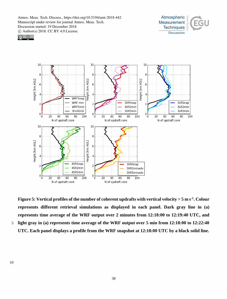
38

Figure 5: Vertical profiles of the number of coherent updrafts with vertical velocity > 5 m s-1. Colour

represents different retrieval simulations as displayed in each panel. Dark gray line in (a)

represents time average of the WRF output over 2 minutes from 12:18:00 to 12:19:40 UTC, and

light gray in (a) represents time average of the WRF output over 5 min from 12:18:00 to 12:22:40 5

UTC. Each panel displays a profile from the WRF snapshot at 12:18:00 UTC by a black solid line.

10


39

Figure 6: Vertical profiles of updraft fractions with different thresholds of 5 m s-1 (solid lines) and

10 m s-1 (dashed lines) for the entire retrieval domain (a – e) and a center region shown as a box in

Fig. 2 (f). Color represents different retrieval simulations as displayed in each panel.

5


40

Figure 7: Vertical profiles of convective mass flux with different updraft thresholds of 5 m s-1 (solid

lines) and 10 m s-1 (dashed lines) for the entire retrieval domain (a–e) and a center region shown as

a box in Fig. 2 (f). Color represents different retrieval simulations as displayed in each panel.

5


41

Figure 8: Same as Figure 7, but for mean updraft. Color representation is same as Figure 7.

5


42

Figure 9: Vertical cross sections of vertical velocity for an updraft core from 3XR (a-d) and 3LR

(e-h) wind retrieval simulations with 2-min and 5-min VCPs. Top raw and bottom raw display non-

advection correction and advection-corrected retrievals, respectively. A selected updraft core is the

same as shown in Fig. 3. 5


investigation of observational error sources in multi ... · since the pioneer ing work of...

Documents