Louisiana State UniversityLSU Digital Commons

LSU Doctoral Dissertations Graduate School

2013

Investigations of the initiation of motion in aeoliantransportBrandon L. EdwardsLouisiana State University and Agricultural and Mechanical College

Follow this and additional works at: https://digitalcommons.lsu.edu/gradschool_dissertations

Part of the Social and Behavioral Sciences Commons

This Dissertation is brought to you for free and open access by the Graduate School at LSU Digital Commons. It has been accepted for inclusion inLSU Doctoral Dissertations by an authorized graduate school editor of LSU Digital Commons. For more information, please contactgradetd@lsu.edu.

Recommended CitationEdwards, Brandon L., "Investigations of the initiation of motion in aeolian transport" (2013). LSU Doctoral Dissertations. 3312.https://digitalcommons.lsu.edu/gradschool_dissertations/3312

INVESTIGATIONS OF THE INITIATION OF MOTION IN AEOLIAN TRANSPORT

A Dissertation

Submitted to the Graduate Faculty of the Louisiana State University and

Agricultural and Mechanical College in partial fulfillment of the

requirements for the degree of Doctor of Philosophy

in

The Department of Geography and Anthropology

By Brandon L. Edwards

B.S., Louisiana State University, 2003 M.S., Louisiana State University, 2006

August 2013

ii

TABLE OF CONTENTS ABSTRACT ............................................................................................................................... iii 1. INTRODUCTION .................................................................................................................... 1 2. SMALL-SCALE VARIABILITY IN SURFACE MOISTURE ON A FINE-GRAINED BEACH: IMPLICATIONS FOR MODELING AEOLIAN TRANSPORT .............................................................. 8 3. COMPARISON OF SURFACE MOISTURE MEASUREMENTS TO DEPTH-INTEGRATED MOISTURE MEASUREMENTS ON A FINE-GRAINED BEACH ...................................................... 23 4. SIMPLE INFRARED TECHNIQUES FOR MEASURING BEACH SURFACE MOISTURE .................. 46 5. PREDICTING THRESHOLD SHEAR VELOCITY FOR INTIATION OF AEOLIAN TRANSPORT OF QUARTZ SANDS AS A FUNCTION OF MASS AND GRAIN SIZE-RANGE ....................................... 66 6. FIELD MEASURMENTS OF AEOLIAN TRANSPORT THRESHOLDS ........................................... 84 7. SUMMARY AND CONCLUSIONS ........................................................................................ 105 APPENDIX 1: PERMISSION TO REPRODUCE CHAPTER 3 IN THIS DISSERTATION ..................... 108 APPENDIX 2: PERMISSION TO REPRODUCE CHAPTER 2 IN THIS DISSERTATION ..................... 109 APPENDIX 3: PERMISSION TO REPRODUCE CHAPTER 4 IN THIS DISSERTATION .................... 115 VITA ..................................................................................................................................... 122

iii

ABSTRACT

This dissertation is an investigation of the initiation of motion in aeolian sediment transport. The

chapters within address transport thresholds for dry sands and spatiotemporal variability of

surface moisture on natural beaches, both critical concerns for the study of aeolian processes.

Results indicate a new model of transport threshold conditions provides substantial

improvement in predictive capability. Field measurements closely match model predictions. In

addition, results indicate that small scale variability and near surface gradients of surficial

moisture are important components to aeolian systems. New techniques for measuring beach

surface moisture provide improved accuracy over previous approaches.

1

1. INTRODUCTION

This dissertation presents investigations of the initiation of motion in aeolian transport.

At the initiation of motion in dry sands aerodynamic forces must overcome inertial forces, and

almost exclusively, the threshold condition is framed as a balance between these forces

following the work of Bagnold (1936). Since Bagnold’s seminal work (1936) many studies have

reported observations and analyses of the transport threshold for dry sands (e.g., Chepil, 1945;

Kawamura, 1951; Zingg, 1953; Chepil, 1959; Belly, 1964; Kadib, 1965; Lyles and Krauss, 1971;

Lyles and Woodruff, 1972; Greeley et al., 1973; Greeley et al., 1976; Iversen et al., 1976; Logie

1981; Iverson and White, 1982; Logie 1982, McKenna Neuman and Nickling, 1989; Cornelis and

Gabriels, 2004). However, the resulting models predict a wide range of threshold values and

observations often do not agree between studies. Thus, there is a clear lack of a confident basis

for predicting aeolian transport thresholds for even the simplest conditions, and this lack

fundamentally limits our understanding of aeolian processes and our ability to model mass flux

at any range of spatiotemporal scale (Sherman et al., 1998; Sherman et al., 2012).

In addition to the inertial force, any cohesive forces associated with intergranular

moisture will require a corresponding increase in the aerodynamic force required to initiate

transport (Belly, 1964; McKenna Neuman and Nickling, 1989; Cornelis and Gabriels, 2003). A

number of studies have addressed the effects of surface moisture content on thresholds of

motion (e.g. Akiba, 1933; Chepil, 1956; Belly, 1964; Bisal and Hsieh, 1966; Kawata and Tsuchiya,

1976; Azizov, 1977; Horikawa et al., 1982; Logie, 1982; Hotta et al.; 1984; Sarre, 1988; McKenna

Neuman and Nickling, 1989; Gregory and Darwish, 1990; Ismailov et al., 1991; Shao et al., 1996;

Cornelis et al., 2004; Davidson-Arnott et al., 2008), but experimental results and models

predictions of moist sand thresholds again vary widely for a given set of conditions (Horikawa et

al., 1982; Namikas and Sherman, 1995; Cornelis and Gabriels, 2003). Overall, despite almost 80

2

years of aeolian research, no consensus on threshold conditions for a given sand size or set of

environmental conditions has been developed (Horikawa et al., 1984; Sarre, 1987; Cornelis and

Gabriels, 2003), and the initiation of motion remains a key source of uncertainty for modeling

aeolian systems.

In response to this problem, this dissertation focuses on improving understanding of the

transport threshold for dry sands, and also advancing knowledge of spatiotemporal variability in

surficial moisture, a key limiting factor for rates of aeolian transport. An additional original

intent of this work was to extend the studies of dry sand thresholds to moist sands, but despite

a prolonged field presence the conditions encountered were not sufficient to induce transport

of moist sands. Thus, the studies presented here are somewhat discrete, but each study makes a

significant contribution to our understanding of critical controls on aeolian transport thresholds,

particularly in the coastal environment.

Chapters 2-4 of this dissertation focus on improving our understanding of

spatiotemporal variability of surficial moisture on natural beaches, and developing improved

techniques to quantify surficial moisture on beaches. Perhaps one of the most critical concerns

involved in understanding the role that moisture plays in transport processes is that application

of much available theoretical work to field situations is not currently possible. Spatiotemporal

variability in surficial moisture on beaches is not well understood, which has prompted a

number of recent studies seeking to more fully document and explain beach moisture dynamics

(e.g. Atherton et al., 2001; McKenna Neuman and Langston, 2003, 2006; Zhu, 2006; Darke and

McKenna Neuman, 2008; Darke et al., 2009; Delgado-Fernandez et al., 2009; Namikas et al.,

2010; Schmutz and Namikas, 2012). However, much of this work has been focused on meso-

scale monitoring and there is still a need to investigate variability over the small scale, as well as

3

near surface gradients in moisture with depth. For these purposes, improved technology is

needed that can accurately measure moisture at the sediment surface.

Chapter 2 discusses small-scale variability of near-surface moisture and its potential

effects on estimates of the total beach surface area available for transport. This work was

designed to assess whether or not we need to incorporate small-scale variability, which is

readily apparent in the field on many beaches, when scaling up to meso-scale modeling and

sediment budgeting efforts. Chapter 3 presents a comparison of depth-integrated and surface

measurements of moisture designed to assess potential errors associated with the use of depth-

integrated measurements and to provide a key incremental step in understanding variability in

near-surface moisture gradients.

Chapters 3 and 4 both present new techniques designed to collect measurements of

moisture at the sediment surface. Accurate measurements of moisture in the top few layers of

grains are needed to study surficial moisture in terms of aeolian transport under field

conditions, but current techniques are inadequate for this goal. One of the most significant

hindrances to accurate quantification of the relationship between near-surface moisture and

transport thresholds and mass flux is this lack of suitable measurement techniques. Both

Chapters 3 and 4 discuss current trends in moisture measurement technologies and assess the

use of a handheld spectroradiometer for measuring moisture at the surface. Chapter 4 presents

data from the field test of an inexpensive narrow band radiometer designed for this purpose as

part of this dissertation.

Chapters 5 and 6 address uncertainty regarding transport thresholds for dry sands.

Chapter 5 presents a new model of threshold conditions developed through a re-examination of

observations reported in previous research. The new model differs from previous approaches in

that it defines threshold conditions as a function of the grain-size range as well as grain mass.

4

The potential importance of grain-size range has been noted by several researchers (e.g., Grass,

1971; Logie, 1981; Gerety and Slingerland, 1983; Namikas and Sherman, 1995; Davidson-Arnott

et al., 2008), but this parameter has not previously been explicitly included in a model of the

threshold condition. Further, by using a grain size distribution that is based on grain mass rather

than diameter to represent grain size, and relating threshold directly to the mass of a

representative grain, the approach developed here represents a significant theoretical

departure from the traditional approaches. It also provides substantially improved predictive

accuracy of aeolian transport thresholds. Chapter 6 presents results from a series of field

experiments designed to validate the new threshold model. It shows that field results agree very

well with model predictions for sands from the field sites.

1.1 References

Akiba M. 1933. Relation between moisture content in sand and the critical wind velocity when sand begins to move. Journal of Agricultural Engineers Society Japan 5, 157-174.

Atherton RJ, Baird AJ, Wiggs GFS. 2001. Inter-tidal dynamics of surface moisture content on a meso-tidal beach. Journal of Coastal Research 17, 482-489.

Azizov A. 1977. Influence of soil moisture in the resistance of soil to wind erosion. Soviet Soil Science 1, 105-108.

Bagnold RA, 1936. The movement of desert sand. Proceedings of the Royal Society of London

A157: 594-620.

Belly P-Y. 1964. Sand Movement by Wind. Technical Memorandum 1, U.S. Army Corps of Eng CERC, 38p.

Chepil WS. 1956. Influence of Moisture on Erodibility of Soil by Wind. Soil Science Society of America Proceedings 20, 288-292. Chepil, WS. 1959. Equilibrium of soil grains at threshold of movement by wind. Soil Science Society Proceedings 23, 422-428.

5

Greeley R, Iversen JD, Pollack JB, Udovich N, White B. 1973 Wind tunnel studies of Martian aeolian processes. Proceedings of the Royal Society of London. Series A, Mathematical and Physical Sciences, 331-360. Greeley R, White B, Leach R, Iversen JD, Pollack J. 1976. Mars: Wind friction speeds for particle movement. Geophysical Research Letters 3, 417-420. Gregory JM, Darwish MM. 1990. Threshold friction velocity prediction considering water content. ASAE Paper No. 902562, American Society of Agricultural Engineering,St Joseph, 16 p. Cornelis WM, Gabriels D. 2003. The effect of surface moisture on the entrainment of dune sand

by wind, an evaluation of selected models. Sedimentology 50, 771-790.

Cornelis WM, Gabriels D, Hartmann R. 2004. A Conceptual Model to Predict the Deflation Threshold Shear Velocity as Affected by Near-Surface Soil Water, I. Theory. Soil Science Society of America Journal 68, 1154-1161. Cornelis WM, Gabriels D, Hartmann R. 2004. A parameterization for the threshold shear velocity

to initiate deflation of dry and wet sediment. Geomorphology 59, 43–51.

Darke I, Davidson-Arnott RGD, Ollerhead J. 2009. Measurement of Beach Surface Moisture Using Surface Brightness. Journal of Coastal Research 25, 248-256. Darke I, McKenna Neuman C. 2008. Field study of beach water content as a guide to wind erosion potential. Journal of Coastal Research 24, 1200-1208. Davidson-Arnott RGD, Yang Y, Ollerhead J, Hesp P.A, and Walker IJ. 2008. The effects of surface moisture on aeolian sediment transport threshold and mass flux on a beach. Earth Surface Processes and Landforms 33, 55-74. Davidson-Arnott RGD, MacQuarrie K,Aagaard T. 2005. The effect of wind gusts, moisture content and fetch length on sand transport on a beach. Geomorphology 68, 115-129. Davidson-Arnott RGD, Bauer BO. 2009. Aeolian sediment transport on a beach: Thresholds, intermittency, and high frequency variability. Geomorphology 105, 117-126. Delgado-Fernandez I, Davidson-Arnottt RGD, Ollerhead J. 2009. Application of a Remote Sensing Technique to the Study of Coastal Dunes. Journal of Coastal Research 25, 1160-1167. Hotta S, Kubota S, Katori S, Horikawa K. 1984. Sand transport by wind on a wet sand surface. In Proceedings of the 19th International Coastal Engineering Conference, Houston, Texas, American Society of Civil Engineers, New York, 1265–1281. Horikawa, K., S. Hotta, and S. Kubota, 1982. Experimental study of blown sand on a wetted sand surface. Coastal Engineering in Japan 25, 177-195.

6

Ismailov MI, Ismailov MM, Mirzazhanov KM. 1991. Proneness of soils to wind erosion as a

function of moisture content and wind speed. Soviet Soil Science 23, 66-68.

Iversen JD, Greeley R,Pollack JB. 1976. Windblown dust on earth, Mars and Venus. Journal of Atmospheric Sciences 33, 2425-2429.

Iversen JD, White B. 1982. Saltation threshold on earth, mars and venus. Sedimentology 29, 111-119. Kawata Y, Tsuchiya Y. 1976. Influence of water content on the threshold of sand movement and the rate of sand transport in blown sand. Proceedings of the Japanese Society of Civil Engineering 249, 195-100. Logie M, 1981. Wind tunnel experiments on dune sands. Earth Surface Processes and Landforms 6, 365-374. Logie,M, 1982. Influence of roughness elements and soil moisture on on the resistance of sand to wind erosion. Catena, Supplement 1, 161-174. McKenna Neuman CL, Langston G. 2003. Spatial analysis of surface moisture content on beaches subject to aeolian transport. Proceedings of the Canadian Coastal Conference (Kingston, Ontario, Canada), 1-10. McKenna Neuman CL, Langston G. 2006. Measurement of water content as a control of particle entrainment by wind. Earth Surface Processes and Landforms, 31, 303-317. McKenna Neuman CL, Nickling WG. 1989. A theoretical and wind tunnel investigation of the

effect of capillary water on the entrainment of sediment by wind. Canadian Journal of Soil

Science 69, 79-96.

Namikas SL, Sherman DJ. 1995. A review of the effects of surface moisture content on aeolian

sand transport. In, Desert Aeolian Processes, Tchakerian VP (ed). Chapman and Hall, New York;

269-293.

Namikas SL, Edwards BL, Bitton MCA, Booth JL, Zhu Y. 2010. Temporal and spatial variabilities in the surface moisture content of a fine-grained beach. Geomorphology 114, 303-310. Sarre RD. 1988. Evaluation of Aeolian sand transport equations using intertidal zone measurements, Saunton Sands, England. Sedimentology 35, 671-679.

Shao Y, Raupach MR, Leys JF. 1996. A model for predicting aeolian sand drift and dust entrainment on scales from paddock to region. Australian Journal of Soil Research 34, 309-342. Sherman DJ, Jackson DWT, Namikas SL, Wang J. 1998. Wind-blown sand on beaches, an evaluation of models. Geomorphology 22, 113-133.

7

Sherman DJ, Li B. 2012. Predicting aeolian sand transport rates: A reevaluation of models.

Aeolian Research 3, 371-378.

Zingg, A. W., 1953. Wind tunnel studies of the movement of sedimentary material. Proceedings of the 5th Hydraulics Conference, State University of Iowa Studies in Engineering Bulletin 34, 111-135.

8

2. SMALL-SCALE VARIABILITY IN SURFACE MOISTURE ON A FINE-GRAINED BEACH:

IMPLICATIONS FOR MODELING AEOLIAN TRANSPORT1

2.1 Introduction

It has long been recognized that water in intergranular pore spaces can produce

cohesive forces, and that these forces can in turn retard or prevent aeolian sediment transport

(Haines, 1925; Chepil, 1956; Belly, 1964; Svasek and Terwindt, 1974, McKenna Neuman and

Nickling, 1989; Namikas and Sherman, 1995; Davidson-Arnott et al., 2008). Physically based

models of this effect are available at the scale of individual grains (e.g., McKenna Neuman and

Nickling, 1989). However, the influence of intergranular moisture on aeolian transport at

intermediate spatial scales (hundreds of meters to a few kilometers) is poorly understood due to

a lack of knowledge regarding the spatial and temporal distribution of surface moisture on real

world beaches. New measurement technology, in the form of compact, minimally destructive,

and rapid moisture content sensors, has recently enabled workers to obtain rapid, repetitive

measurements covering relatively large areas (typically grids covering a few tens to hundreds of

square meters). Consequently, recent studies have begun to provide insight into the nature of

spatial and temporal variability in the surface moisture content of beaches (Atherton et al.,

2001; Wiggs et al., 2004; Yang and Davidson-Arnott, 2005; Zhu, 2007; Davidson-Arnott et al.,

2008).

To date, the sample spacing used to map beach surface moisture content has been

relatively coarse, typically involving sampling intervals on the order of 5 m (e.g. Zhu, 2007;

Davidson-Arnott et al., 2008). However, we have observed substantive variation in moisture

content at much smaller spatial scales on the fine-grained beaches of the northern Gulf of

Mexico. Informal observations during field work for Zhu (2007) frequently showed repeatable

moisture content differences exceeding 10% (by weight) over distances of centimeters to tens of

1 Reproduced with permission of Earth Surface Processes and Landforms. See APPENDIX I

9

centimeters. These observations led to concern regarding how well actual surface moisture

distributions are represented by a relatively coarse grid and motivated the present study.

This paper addresses two main issues. First, it seeks to quantify and characterize the

nature of small-scale (< 1 m) variations in surface moisture content on a beach. The second goal

is to assess the implications and potential influence of small-scale moisture variability for

aeolian transport at larger scales. We focus specifically on the relative portion of beach area that

would be available or unavailable for transport in order to examine the latter issue, as

determined by whether local moisture content is above or below a specified threshold level

above which transport is assumed to be prevented.

2.2 Study Site and Field Methods

Study Site

Field experiments were conducted at Padre Island National Seashore, on Padre Island,

Texas (latitude and longitude approximately 27.48º N 97.28º W). The beach consists of very-well

sorted, fine to very fine quartz sands, with a mean grain size of approximately 0.14 mm. The

beach at Padre Island is generally dissipative to intermediate, with low wave energy levels and a

micro-tidal range (typically < 1 m). The berm at the study site was about 40-60 m in width,

relatively flat (1-3o), and graded into a vegetated foredune ridge approximately 1 to 2 m in

height at its landward edge (Figure 2.1).

The water table is very shallow at this site (typically about 70-90 cm deep at the

foredune toe, and progressively shallower in the seaward direction), and the strong capillary

forces associated with the fine sediments are capable of drawing moisture to the surface over

large portions of the berm. Thus, high surface moisture levels are maintained even during

extended dry periods (Zhu, 2007). We have observed aeolian transport events on numerous

10

Figure 2.1 Study site at North Padre Island, TX. Viewed from the foredune.

occasions at this beach, and they are characteristically highly variable both in space (being

restricted mainly to higher, drier zones close to the foredune) and time (it is common for

transport to decrease or stop although wind speeds remain constant or increase, as the

uppermost layer of dry material is stripped away exposing the damper sediment beneath). We

therefore believe variability in surficial moisture content exerts a critically important control on

aeolian processes in this and similar environments.

Surface Moisture Measurements

Surface moisture measurements were made with a Type ML2x Theta probe (Delta-T

Devices, Cambridge, England). The length of the probe sensor rods, which is 60 mm as supplied

by the manufacturer, was an issue of concern for our application. The resulting measurements

are integrated over too great a depth to be considered a reasonable approximation of the

‘surface’ moisture content. Thus, the unit used here was modified following Yang and Davidson-

11

Arnott (2005) to reduce the active sensor length to 14 mm. The modification involves simply

encasing a portion of the sensor rods in dielectric foam. Yang and Davidson-Arnott reported no

significant loss of accuracy using 20 mm of exposed probe length, and Schmutz (2007), in a

comparative study testing different variations of this method (e.g. probe length, grain size),

found that when only 15 mm of exposed probe length, the standard error of measurement only

increased by 0.9 % moisture content and precision was not significantly affected.

A square aluminum guide was used to control sampling locations in order to standardize

the spatial pattern of measurements. Measurements were collected at 10 cm intervals over a 40

cm by 40 cm grid providing a data set comprised of 25 individual measurements. The specific

locations on the beach where these grid data sets were collected were determined by trial and

error, so as to represent the entire range of probe output (approximately 0-750 mV from

completely dry to fully saturated sediment). Basically, the probe was inserted into the beach

surface and the output read, repeatedly. When a reading fell into a part of the output range for

which no data had been collected, the frame was placed around that area and a full 25 point

data set collected. In total, 44 grid data sets were collected between 07/27/2006 and

07/30/2006. All measurements were collected between approximately 13:00 and 16:00 hrs.

Probe Calibration

The manufacturer supplies a 3rd order polynomial calibration for the Theta probe that

produces values of volumetric moisture content (Delta-T Devices, 1999). The more common

convention, however, when dealing with surface moisture on beaches, is to report gravimetric

moisture content. Accurate values of bulk density are required to convert between the two.

Thus, in order to avoid a potential source of error during conversion, a site-specific calibration

was designed to relate probe output to gravimetric moisture content (Figure 2.2).

12

Figure 2.2 Calibration curve for moisture probe. R2 value ≈ 0.97.

We targeted calibration points at small intervals that represented the full range of probe

output (approximately 0 to 750 mV). To accomplish this, surface moisture measurements were

taken at arbitrary locations on the beach. When a targeted output was observed, a circular core

of the sediment that produced the reading was collected (65 mm diameter x 14 mm depth,

equivalent to the sampling volume of the probe). The samples were then sealed in canisters and

transported back to the laboratory for standard gravimetric moisture content determination.

Calibration curves for the Theta probe presented in coastal literature have varied from

linear (Yang and Davidson-Arnott, 2005) to polynomial (Atherton et al., 2001 and Schmutz,

2007). According to Schmutz (2007) and Yang and Davidson-Arnott (2005), salinity and grain

13

size are two factors that contribute to this variability. In this study, we chose to use a 6th order

polynomial (R2 = 0.97) because it produced the lowest standard error (1.45%) while still

including all of the measurement points.

Considering the probe modification (≈ 75% reduction in length), we felt a 0.45% increase

in standard error over the manufacturer supplied calibration (1% error) was acceptable. One

issue was the relatively unresponsive range between about 200 and 350 mV. Because there was

no a priori knowledge of the calibration before the experiment, this caused there to be a large

number of measurement sets with mean moisture contents between 6 and 7% (Table 2.1).

However, the range of standard deviations within these sets was very low (0.4 – 0.8% moisture

content), so there was not a significant effect on subsequent analyses.

Table 2.1 Mean, standard deviation, and range in surface moisture contents for grid data set.

Data Set Mean SD Range Data Set Mean SD Range

27 0.0 0.0 0.2 38 8.0 2.0 6.9 25 0.0 0.1 0.2 44 9.7 2.6 8.3 22 0.0 0.1 0.2 35 10.0 2.6 10.2 43 0.3 0.1 0.4 33 10.1 1.9 8.1 37 0.8 0.2 1.0 20 10.2 1.9 8.2 21 0.8 0.6 2.6 32 11.1 1.8 6.3 4 4.1 1.3 5.0 6 14.1 3.5 12.0 39 5.4 1.0 3.7 40 15.1 4.1 14.2 1 5.4 1.2 3.9 7 15.7 1.9 7.5 36 5.4 0.8 2.5 30 15.9 2.0 8.0 5 5.9 0.9 2.6 10 16.2 3.5 11.5 3 6.4 0.7 3.5 9 16.9 2.9 12.7 42 6.4 0.4 1.6 28 17.0 1.9 7.3 2 6.5 0.4 1.7 8 21.9 2.2 8.9 41 6.6 0.2 1.2 12 23.8 0.5 1.9 26 6.6 0.4 1.9 13 24.0 0.3 1.2 18 6.7 0.2 1.0 31 24.1 0.3 1.1 24 6.7 0.3 1.1 11 24.2 0.3 1.2 23 6.7 0.3 1.0 34 24.3 0.2 1.0 19 6.8 0.5 1.9 15 24.4 0.1 0.5 17 6.8 0.8 3.5 14 24.5 0.1 0.3 16 6.9 0.5 1.6 29 25.2 0.5 1.7

14

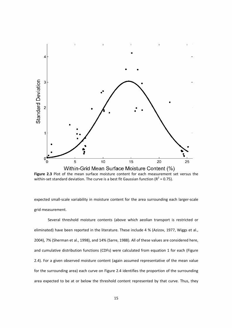
2.3 Results and Analysis

Measured Small-Scale Variability

Table 2.1 provides the mean (x), standard deviation (σ), and range (difference between

highest and lowest moisture content) for each grid data set, ordered by the mean within-grid

surface moisture content. Mean moisture contents ranged from 0 to approximately 25 %

gravimetric moisture content, representing conditions from completely dry (near the dune toe)

to fully saturated (swash zone). These data show that small-scale variability in moisture content

is smallest for very dry sediments and increases fairly consistently with higher moisture levels,

up to a content of about 15 %. Variability then begins to decrease, becoming minimal once again

for very wet sediments. The relationship between mean moisture content and the magnitude of

small-scale variability (Figure 2.3) was found to be reasonably well approximated (R2 = 0.75) by a

Gaussian distribution:

σ = 3.04*exp(-((x-14.56)/6.83)^2) (2.1)

where σ is the standard deviation, and x is the mean moisture content of a grid data set.

Estimating Beach Area Available for Aeolian Transport

The specific issue at hand is to model the proportion of beach area that will have

moisture contents above or below a given threshold level, taking into account the small-scale

variability described above. In order to accomplish this, the assumption is made that each

moisture measurement reported for larger-scale grids (e.g., Zhu, 2007, Davidson-Arnott et al.,

2008) approximates the mean content for the immediately surrounding area. Given this

assumption, these larger-scale grid measurements can then be considered comparable to the

grid data set mean values reported above, and equation 1 can be used to represent the

15

Figure 2.3 Plot of the mean surface moisture content for each measurement set versus the within-set standard deviation. The curve is a best fit Gaussian function (R2 = 0.75).

expected small-scale variability in moisture content for the area surrounding each larger-scale

grid measurement.

Several threshold moisture contents (above which aeolian transport is restricted or

eliminated) have been reported in the literature. These include 4 % (Azizov, 1977, Wiggs et al.,

2004), 7% (Sherman et al., 1998), and 14% (Sarre, 1988). All of these values are considered here,

and cumulative distribution functions (CDFs) were calculated from equation 1 for each (Figure

2.4). For a given observed moisture content (again assumed representative of the mean value

for the surrounding area) each curve on Figure 2.4 identifies the proportion of the surrounding

area expected to be at or below the threshold content represented by that curve. Thus, they

16

Figure 2.4 Cumulative distribution functions for each threshold value. Curves represent the proportion of surrounding area expected to be at or below the critical threshold moisture content for a given mean moisture content. Dotted lines refer to the example in the text.

indicate the proportion of the surrounding area expected to be available for aeolian transport.

Given a surface moisture measurement of 15%, for example, the curve for the 14% threshold

indicates that about 39% of the surrounding area would be expected to have moisture levels at

or below the threshold value (Figure 2.4). In this case, a substantial portion of the surrounding

area would be available for transport, despite an observed moisture content exceeding the

critical threshold. Similarly, measurements below threshold do not necessarily indicate that the

entire surrounding area is available for transport.

It is worth noting here that the magnitude of this effect is greater for higher threshold

values. Consider, for example, the case of a 4% threshold value and a measured content of 5%

17

(1% above the threshold value, as in the previous example). In this case only about 2% of the

surrounding area would be expected to have moisture contents at or below the threshold

(Figure 2.4).

Application of the Model to a Typical Beach

The final step needed to assess the potential significance of small-scale variations in

surface moisture for aeolian transport is to examine the model output in the context of real-

world moisture distributions. From Figure 2.4 it is apparent that only areas of beach surface that

exhibit surface moisture contents close to the threshold value will be significantly influenced by

small-scale variability (specifically how close depends on the selected threshold value, as shown

in the previous section). Hence, the question is how much of the actual beach surface has

moisture levels that are close enough to a given threshold for small scale variability to become a

significant issue.

To examine this issue, six larger-scale surface moisture maps (Figure 2.5) from the same

study site are used. The larger-scale maps were derived from a 20 m (alongshore) by 60 m

(cross-shore) grid with 5 m spacing between sample points (Zhu, 2007). The measured moisture

contents were interpolated (linear interpolation) onto a 0.5 by 0.5 meter grid so that each cell in

the interpolation would be of equal area to the grid data set used previously to characterize

small-scale variability.

To provide initial estimates of the proportion of beach area available for aeolian

transport, the number of cells with moisture levels equal to or smaller than each of the three

threshold values were counted and divided by the total number of cells in the interpolated

moisture maps. Next, the CDFs from Figure 2.4 were used to model small-scale variability within

each cell and the beach area available for transport was recalculated for comparison.

18

As shown in Table 2.2, when small-scale variability in surface moisture is taken into

account there are only minimal changes in the estimated area of beach surface available for

transport. The maximum change in available beach surface area exceeded 1% in only two cases.

This does not seem particularly worrisome, especially when considered in light of the many

potential sources of error generally involved in sediment transport modeling. Interestingly, the

largest influence of small scale variability (when averaged for all six maps) does not occur with a

threshold value of 14%, despite the fact that the CDFs in Figure 2.4 suggest a stronger influence

should be found with a higher threshold value. This indicates that the actual surface moisture

distributions found at this site are an important factor in determining the significance of small

scale variability to aeolian transport.

2.4 Summary and Conclusions

The two goals of this paper were to quantify small-scale variations in surface moisture

on a fine grained beach and to explore the significance of those results in terms of modeling

beach surface area available to aeolian transport. Variability tended to be smallest for very dry

or very wet sediments and largest at intermediate moisture levels, following an approximately

normal distribution. It was found that surface moisture content can be highly variable over small

areas, with differences of up to about 14% by weight occurring within the 0.5 m2 grid data set.

These results indicate that there is a potential for disparity between observed surface moisture

values in the field and actual surface moisture conditions, particularly in the mid ranges of

possible moisture contents. For example, if the actual mean surface moisture content for a

small area was 10 %, according to Equation 1, there is a 32 % chance that an observed value

would be at least ± 2 %. Potential for error is greater when taking into account the range of

observed values in a small area from Table 2.2.1. Measurement set 35, for example, had a mean

19

Figure 2.5 Moisture maps for assessment of input of impact of small-scale variability (data from Zhu 2007). The top of each map coincides with the dune toe and the bottom falls within the swash zone. Data were collected at 5 m intervals on a 20 m by 60 m grid.

20

Table 2.2 Influence of small-scale variability (SSV) on beach area available for aeolian transport.

Area Available for Transport (%)

4% Threshold

7% Threshold 14 % Threshold

Map # Date Without SSV With SSV Difference Without SSV With SSV Difference Without SSV With SSV Difference

MS 1 7/29/2005 35.2 35.4 0.2 51.9 52.7 0.8 69.8 68.6 -1.2

MS 2 7/30/2005 49.1 49.2 0.1 65.1 65.2 0.1 74.8 74.5 -0.3

MS 3 7/30/2005 31.1 31.1 0.0 40.5 41.0 0.6 48.6 48.2 -0.4

MS 4 8/2/2005 49.4 49.3 -0.1 54.0 55.1 1.1 71.5 71.7 0.2

MS 5 7/30/2005 43.5 43.2 -0.3 53.5 54.3 0.8 67.1 66.6 -0.6

MS 6 7/31/2005 46.1 46.1 -0.1 56.0 56.9 0.9 72.0 71.7 -0.3

Average: 0.0 0.7 -0.4

21

moisture level of 10.0 %, and the range was 10.2 %. Such disparities could potentially cause

difficulties in research involving surficial moisture conditions, e.g. endeavors to establish critical

moisture values for transport.

To address the second goal of this paper, cumulative distribution functions were used to

model small-scale variations in surficial moisture in the context of three ‘threshold’ values

suggested in the literature (4%, 7%, and 14%). It was found that the larger the specified

threshold level, the greater the significance of small-scale variability in terms of beach area

available for aeolian transport (i.e. at or below the threshold moisture content). These functions

were used to model small-scale variability in surface moisture distributions mapped at the same

site but on a much coarser grid. It was found that the change in the estimated area available for

aeolian transport resulting from consideration of small-scale variability was negligible, typically

less than 1%. Thus, at this site small-scale variability does not have significant implications for

aeolian transport modeling in terms of the surface area available to transport, and a relatively

coarse sampling grid (5m) provides an adequate characterization of beach moisture contents for

this purpose. It should be noted, however, that this analysis did not consider the effects of

small-scale variability to other potentially significant transport parameters, such as fetch length

or beach drying time. Further work should be conducted to investigate other potential impacts

of variability in surface moisture.

2.5 References

Atherton RJ, Baird AJ, Wiggs GFS. 2001. Inter-tidal dynamics of surface moisture content on a meso-tidal beach. Journal of Coastal Research 17, 482-489. Azizov MT. 1977. Influence of soil moisture on the resistance of soil to wind erosion. Pochvovedeniye 1, 102-108. Belly P-Y. 1964. Sand Movement by Wind. Technical Memorandum 1, U.S. Army Corps of Eng CERC, 38p.

22

Chepil WS. 1956. Influence of soil moisture on erodibility of soil by wind. Soil Science Society of

America Proceedings 20, 288-292. Davidson-Arnott RGD, Yang Y, Ollerhead J, Hesp PA, Walker IJ. 2008. The effects of surface moisture on aeolian sediment transport threshold and mass flux on a beach. Earth Surface

Processes and Landforms 33, 55-74. Delta-T Devices. 1999. Theta Probe Soil Moisture Sensor Type ML2x User Manual. Cambridge, United Kingdom, Delta-T Devices, Ltd. Haines WB. 1925. Studies in the physical properties of soils, II. A note on the cohesion developed by capillary forces in an ideal soil. Journal of Agricultural Science 15, 529-535. McKenna Neuman CL, Nickling WG. 1989. A theoretical and wind tunnel investigation of the effect of capillary water on the entrainment of sediment by wind. Canadian Journal of Soil

Science 69, 79-96. Namikas SL, Sherman DJ. 1995. A review of the effects of surface moisture content on aeolian sand transport. In, Desert Aeolian Processes, Tchakerian VP (ed). Chapman and Hall, New York; 269-293. Sarre RD. 1988. Evaluation of Aeolian sand transport equations using intertidal zone measurements, Saunton Sands, England. Sedimentology 35, 671-679. Schmutz PP. 2007. Investigation of utility for Delta-T Theta Probe for obtaining surficial moisture measurements on beaches. Master’s Thesis, Department of Geography & Anthropology, Louisiana State University. Baton Rouge, Louisiana, US. Sherman DJ, Jackson DWT, Namikas SL, Wang J. 1998. Wind-blown sand on beaches, an evaluation of models. Geomorphology 22, 113-133. Svasek JN, Terwindt JHJ. 1974. Measurements of sand transport by wind on a natural beach. Sedimentology 21, 311-322. Wiggs CFS, Baird AJ, Atherton RJ. 2004. The dynamic effects of moisture on the entrainment and transport of sand by wind. Geomorphology 59, 13-30. Yang Y, Davidson-Arnott RGD. 2005. Rapid measurement of surface moisture content on a beach. Journal of Coastal Research 21, 447-452. Zhu Y. 2007. Modeling spatial and temporal variations of surface moisture content and groundwater table fluctuations on a fine-grained beach, Padre Island, Texas. PhD Dissertation, Department of Geography & Anthropology, Louisiana State University.

23

3. COMPARISON OF SURFACE MOISTURE MEASUREMENTS TO DEPTH-INTEGRATED MOISTURE

MEASUREMENTS ON A FINE-GRAINED BEACH2

3.1 Introduction

The measurement of surface moisture on beaches is a fundamental component of field

studies that seek to define and model beach groundwater pathways and reservoirs (e.g., Turner,

1993; Atherton et al., 2001; Namikas et al., 2010), or investigate the role of surface moisture in

aeolian transport processes (e.g., Sherman et al., 1998; Wiggs et al., 2004; Davidson-Arnott et

al., 2008; Oblinger and Anthony, 2008; Bauer et al., 2009; Edwards and Namikas, 2009; Namikas

et al., 2010; Nield et al., 2011). However, measurement of moisture content at the surface of

the sediment bed is difficult and available techniques are subject to significant limitations.

Traditionally, surface scrapings have been collected to assess surficial moisture conditions, and a

number of more recent studies have employed depth-integrated soil moisture probe

approaches that avoid several key limitations associated with the former. Both of these

approaches quantify moisture integrated over depth to some degree, and consideration of

moisture measurements with regard to aeolian process studies raises the issue of how

accurately depth-integrated sampling represents moisture content at the surface. While the

available literature does not completely assume (through a general lack of warnings to the

contrary) that one can be used to represent the other, data characterizing the level of error

between depth integrated and surface moisture measurements are limited. This information is

certainly important, however, in interpreting results of many oft-cited studies on the effects of

surficial moisture on aeolian transport thresholds and transport rates. This study addresses this

issue through a comparison of depth integrated time domain reflectometry (TDR)

measurements with optical measurements of surface moisture contents obtained with a

portable spectroradiometer on a fine-grained beach.

2 Reproduced with permission of Journal of Coastal Researh. See APPENDIX II

24

Techniques that have been used to measure beach surface moisture can be grouped

into three basic approaches: manual sample extraction, in situ indirect measurement, and

remote sensing techniques. The manual sampling approach involves collecting scrapings or

shallow samples of surface sediment for laboratory analysis (e.g., Sarre, 1988, Kroon and

Hoekstra, 1990; Gares et al., 1996; Nordstrom et al., 1996; Jackson and Nordstrom, 1997,

Sherman et al., 1998; Wiggs et al., 2004; Davidson-Arnott et al., 2005). Subsequent

determination of gravimetric moisture content by weighing, drying, and reweighing the sample

provides a direct measure of moisture content, making this potentially the most accurate

approach, although the depth of sediment collected for analysis has varied significantly between

studies. However, this method is time consuming to an extent that significantly limits the ability

to sample moisture contents across large areas with detailed resolution. Perhaps more

importantly, sample extraction destroys the sediment surface so that the ability to repetitively

sample at a given location (e.g. to document temporal changes) is compromised. Together,

these limitations restrict the utility of this approach for many applications.

There are a number of commercially available in situ soil moisture sensors, including

capacitance probes, neutron probes, and tensiometers. Recently, several studies have reported

in situ measurements of beach surface moisture conducted with a TDR sensor, such as the

Delta-T Theta probe (Atherton et al., 2001; Wiggs et al., 2004; Yang and Davidson-Arnott, 2005;

Davidson-Arnott et al., 2008; Oblinger and Anthony, 2008; Bauer et al., 2009; Davidson-Arnott

and Bauer, 2009; Edwards and Namikas, 2009; Namikas et al., 2010; Schmutz and Namikas,

2011, Nield et al., 2011). This technique overcomes many of the limitations associated with

extraction sampling; measurements can be rapidly collected and the process causes minimal

surface deformation. This allows for collection of large numbers of measurements to

characterize spatial variability, and also allows repeated sampling at a given measurement

25

station to document temporal variability (e.g., Yang and Davidson-Arnott, 2005; Edwards and

Namikas, 2009; Namikas et al., 2010). A weakness, however, lies in the sensor length. As

supplied by the manufacturer, the active length of this type of probe is typically on the order of

a few cm (6 cm for the Theta probe). Thus, measurements are integrated over depth rather than

providing a true ‘surface’ measurement. While this issue can be circumvented somewhat by

modifying the probes to reduce sampling depth (e.g., Tsegaye et al., 2004; Yang and Davidson-

Arnott, 2005; Davidson-Arnott et al., 2008; Bauer et al., 2009; Edwards and Namikas, 2009;

Namikas et al., 2010; Schmutz and Namikas, 2011), the ability of measurements integrated over

even these shallow depths to accurately describe conditions at the surface has been described

sparingly in the literature. Certainly, there is a fundamental assumption that there is some

departure between moisture measured over some depth and the ‘true’ moisture content in the

top few layers of grains (which are of the most importance for beach-aeolian process studies)

because of near-surface vertical moisture gradients. However, field data or discussions

describing the nature of this departure (either directly or indirectly) are currently limited to a

handful of studies and restricted to the lower half of typical gravimetric moisture levels

(approximately 0 to 14%) found on most beaches (e.g. Wiggs et al., 2004; Darke et al., 2009;

Nield et al., 2011).

Partially in response to the concerns described above, several recent studies have

employed remote sensing techniques to attempt to measure and map surface moisture by

relating brightness values derived from digital photography to surface moisture contents

(McKenna Neuman and Langston, 2003, 2006; Darke and McKenna Neuman, 2008; Darke,

Davidson-Arnott, and Ollerhead, 2009; Delgado-Fernandez, Davidson-Arnott, and Ollerhead,

2009, Delgado-Fernandez and Davidson-Arnott, 2011, Delgado-Fernandez, 2011), or using a

terrestrial laser scanner (Nield and Wiggs, 2011, Nield et al., 2011). The remote sensing

26

approach has several distinct advantages. It is non-destructive, it allows for instantaneous

sampling of large areas, and measurements are restricted to the uppermost few layers of grains.

For these reasons, it clearly holds promise, and potentially represents a valuable tool for

characterizing meso-scale spatio-temporal variability in surface moisture. However, results to

date show comparatively large levels of error, with the scatter in calibrations often exceeding

±10% moisture content for a given surface brightness for the digital photography method

(McKenna Neuman and Langston, 2003, 2006; Darke and McKenna Neuman, 2008; Darke,

Davidson-Arnott, and Ollerhead, 2009; Delgado-Fernandez, Davidson-Arnott, and Ollerhead,

2009). Similarly, moisture measurement error for the terrestrial laser scanner (TSL) method used

by Nield and Wiggs (2011) and Nield et al. (2011) increases dramatically as moisture level

increases, and in fact appears to be essentially incapable of discriminating variability in moisture

above levels of 7 or 8%. These errors could be due to the reliance on visible wavelengths for

both methods; according to Lobell and Asner (2002), the primary influence of water in the

visible range of the electromagnetic spectrum is to change refractivity at the soil surface. Thus, it

may be that once moisture content is sufficient to cover soil particles the effect of increased

moisture levels on reflectance decreases significantly, thereby reducing measurement

resolution. This could limit the potential of the visible spectrum for moisture measurement, but

there is much stronger absorption of infrared wavelengths by water, and thus the incorporation

of infrared signals (e.g., Kano, McClure, and Skaggs, 1985; Slaughter, Pelletier, and Upadhyaya,

2001; Lobell and Asner, 2002; Weidong et al., 2002; Weidong et al., 2003; Mouazen et al., 2007)

could enhance the effectiveness of remote sensing approaches.

In this study, we compare two sets of depth-integrated beach surface moisture

measurements obtained from a Theta probe with surface measurements from a handheld

spectroradiometer capable of collecting relative reflectance measurements in the wavelength

27

range of 325 to 1075 nm. The goal of this study is to compare depth-integrated moisture

measurements to conditions at the surface of the bed. As an ancillary component, some

discussion of the spectroradiomter’s utility is provided as a simple introduction to a promising

technology for measuring beach surface moisture.

3.2 Study Site and Methods

Study Site

The study was conducted at Padre Island National Seashore, on Padre Island, Texas, at a

site about 3 km from the northern border of the park (approximately 27.48°N 97.28°W). The

beach sediments consist of very-well sorted, fine to very fine quartz sands, with a mean grain

size of approximately 0.14 mm. The beach is generally multi-barred dissipative to intermediate,

with low wave energy levels and a micro-tidal range (typically <1 m). During the study, the berm

was about 30 m in width and relatively flat (1–3°), and the beach was backed by a 1 to 2 m

foredune ridge.

Instrumentation

The TDR probe used in this study is a Delta-T Theta sensor produced by Delta-T Devices,

Cambridge, UK (Figure 3.3.1). The device is designed to measure the dielectric constant in a

volume of soil. A signal at some frequency is applied to a transmission line, which in turn is

connected to the probe. The transmission line is of fixed impedance, and the impedance of the

probe is determined by the dielectric properties of the surrounding soil (Gaskin and Miller,

1996). The difference in impedance causes a portion of the original signal to be reflected back

toward the source, thus setting up a standing wave of voltage amplitude between the incident

signal and the reflected signal on the transmission line (Gaskin and Miller, 1996). The amplitude

28

of the standing wave can be related to impedance and the soil dielectric constant through a

series of equations (Huang et al., 2004). Manufacturer supplied calibrations can be used to

convert the probe output to volumetric moisture content, or site-specific calibrations can be

conducted by the user to convert output to gravimetric moisture content.

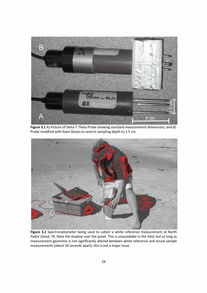
The sensing prongs are approximately 6 cm long and encapsulate a cylinder

approximately 2.5 cm in diameter (Figure 3.1). Some studies have utilized the full length of the

probe (e.g., Atherton, Baird, and Wiggs, 2001; Wiggs et al., 2004). More recently, researchers

have modified these probes to reduce sampling depth by encasing some portion of the probe in

a dielectric foam block, thus reducing the active probe length (Yang and Davidson-Arnott, 2005;

Zhu, 2007; Davidson-Arnott et al., 2008; Bauer et al., 2009; Davidson-Arnott and Bauer, 2009;

Edwards and Namikas, 2009; Namikas et al., 2010; Schmutz and Namikas, 2011) (Figure 3.1).

Although the measurement resolution of the probe decreases as the active probe length is

reduced (Yang and Davidson-Arnott, 2005; Schmutz and Namikas, (2011), there does not seem

to be a significant decrease in accuracy. Schmutz and Namikas (2011) report that reducing the

active probe length to 1.5 cm (from 6 cm at full length) increases the standard error of

measurement from ± 1.0 to ± 1.9 % moisture content.

The spectroradiometer used in this study is an ASD (Analytical Spectral Devices)

FieldSpec® HandHeld (HH) model UV/VNIR (325-1075 nm) spectroradiometer (Figure 3.2). This

device measures radiance or reflectance intensity over the wavelength range of 325 to 1075 nm

at sampling intervals of 1.6 nm. After passing through the fiber optic head, light energy is

directed through a diffraction grating that separates the wavelength components for

29

Figure 3.1 A) Picture of Delta-T Theta Probe showing standard measurement dimensions, and B) Probe modified with foam blocks to restrict sampling depth to 1.5 cm.

Figure 3.2 Spectroradiometer being used to collect a white reference measurement at North Padre Island, TX. Note the shadow over the panel. This is unavoidable in the field, but as long as measurement geometry is not significantly altered between white reference and actual sample measurements (about 10 seconds apart), this is not a major issue.

30

independent measurement by a 512 channel silicon photodiode array. Incident photons are

converted into electrons that are integrated over a user-set interval. Available integration times

range from a few ms (milliseconds) to several minutes (ASD, 2002). Output spectra result from

the average of a user-set number of recorded spectra. For example, if integration time is set to

272 ms, and averaging interval is set to 10, the instrument will output a spectrum every 2.7

seconds. The instrument is controlled by a computer program and output spectra are saved

directly to the computer’s hard drive (Figure 3.2).

For relative reflectance measurements, a reference measurement is collected using a

white reference panel made of a material that approaches 100% reflectivity across the

measurement spectrum. In this case, we used a 3.2 cm diameter, 5 mm thick spectralon diffuse

white reference panel (> 99% reflectance from 400-1500 nm). This allows comparison of

measurements obtained under different ambient lighting conditions (e.g., cloudy vs. sunny), as

long as measurement geometry is not altered, e.g. location with respect to objects (because of

shadows), instrument height, angle to the surface, etc. A ratio of the white reference spectra to

the target spectra produces the relative reflectance spectra. Thus, the spectral signal of the

illumination source is removed, given again that the measurement geometry is not significantly

altered (ASD, 2002). The relative reflectance value of the white panel itself is equal to 1 across

the entire measurement range, and decreases at any particular wavelength as the amount of

light reflected from the target decreases at that wavelength. In the case of these experiments,

higher moisture levels in the sample will absorb more incident energy, and therefore have lower

relative reflectance values.

Conversion of relative reflectance values (R) to absorbance (A) as A=log(1/R) has been

found to remove nonlinearity associated with the absorption process (e.g., Weidong et al.,

2002), and was found here to provide improved results versus the raw relative reflectance

31

Figure 3.3 Laboratory spectroradiometer measurements conducted prior to field study on two separate 3 mm thick samples of moist native Padre Island, Texas sand. Two sets of measurements (closed and open symbols) were conducted periodically as the sand dried and moisture content was established by weighing the sample. Standard error (SE) is reported in percent moisture content.

values. Figure 3.3 shows results from a set of preliminary laboratory tests undertaken to assess

the potential of this device for measuring beach surface moisture in the field. The plot shows

values from the 970 nm wavelength versus gravimetric moisture content from two

approximately 3 mm thick samples of sand initially saturated samples in sediment trays dried

over time, on separate occasions under different lighting and measurement conditions, but

show good agreement. The high R2 value (0.98) and low standard error (0.95% moisture

32

content) indicate that this instrument is potentially well suited to measure beach surface

moisture contents.

There does appear to be some systematic difference between results from the two

separate tests, but this is likely due to small differences in sample thickness, sediment mixture,

and instrument position/measurement angle. Given the relatively high accuracy of the overall

relationship, however, this was considered acceptable, and it was concluded that the

spectroradiometer should provide reasonably accurate moisture values. Further tests on

different sands produced similar results, with R2 values above 0.98 in all cases standard error

less than 1.0% in all cases.

Field Experiments

A total of 16 collocated sets of moisture measurements were obtained spanning the

range of beach sub-environments along a cross-shore transect from dune toe to swash zone as

follows. First, the modified Theta probe was inserted into the beach surface to a depth of 1.5 cm

and a depth-integrated measurement was collected. Immediately afterwards, 6

spectroradiometer readings of the sediment surface were collected, and average values from

these were used for subsequent analyses. The Theta probe has a diameter of 2.5 cm, and the

spectroradiometer collects reflected energy within the diameter of a cone subtending a full

angle of about 25°. Here, the instrument was held approximately 5 cm from the bed, which

provides a comparable sampling diameter of about 2.2 cm. Once the spectra were collected, a

coring tube of the same dimensions as the sampling volume of the Theta probe was used to

extract the sediment sample for determination of gravimetric moisture content. The tube was

inserted into the surface to a depth of 1.5 cm and a trowel was used to seal the bottom of the

tube and retrieve the sample. The extracted samples were immediately sealed in plastic bags

33

and gravimetric moisture contents were determined in the laboratory using standard methods

immediately upon return from the field. A second set of 14 observations was collected using the

same methods, except that the full 6 cm Theta probe length was used and the core depth was

adjusted to correspond.

An additional procedure was conducted to calibrate spectra recorded by the

spectroradiometer to the moisture content of the uppermost layers of grains. Spectra were

collected at 7 locations on the beach that looked visibly different in terms of moisture content,

starting with very dry sediments near the dune toe and moving to nearly saturated sediments

near the swash zone. Again, six spectra were recorded at each location. Following each

measurement, a sediment sample about 1.5 mm thick was removed from the surface using a

stiff plastic card and transported back to the laboratory for gravimetric moisture analysis (Figure

3.4). Unfortunately, two were compromised during transport and only 5 data points were

available for the spectroradiometer calibration. However, given the robust laboratory test

results (Figure 3.3), we deemed this to be acceptable for the scope of this exercise.

3.3 Results and Analysis

Instrument Calibrations

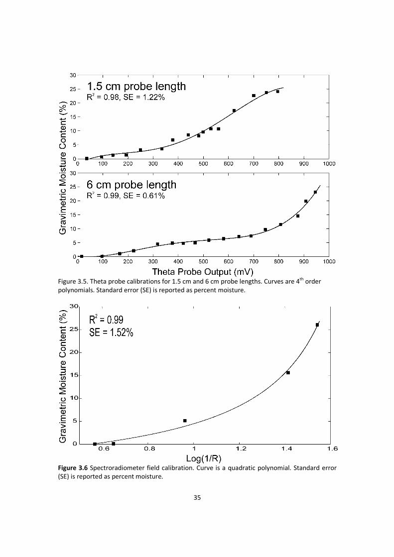
Figure 3.5 shows calibration curves obtained for the 1.5 and 6 cm Theta probe lengths

versus measured gravimetric moisture content. The R2 values for the 1.5 and 6 cm probe lengths

are approximately 0.98 and 0.99, respectively. Note that the standard error is approximately

doubled for the shortened probe length, from 0.61% for the 6 cm probe length to 1.22 % with

the 1.5 cm probe length. The latter is within the range of previously published error values with

the same probe length (e.g., Edwards and Namikas, 2009; Schmutz and Namikas, 2011).

34

Figure 3.4 Sample taken to field calibrate the spectroradiometer. Coin shown for scale is 24 mm in diameter and approximately 1.5 mm thick.

Figure 3.6 shows the field calibration for the spectroradiometer for log(1/R) at a

wavelength of 970 nm versus measured gravimetric moisture content of the 1.5 mm thick

surface samples. The R2 value is approximately 0.99, and the standard error is about ±1.5%

moisture content. This value is somewhat higher than that obtained in preliminary laboratory

experiments (Figure 3.3), but still similar to published levels of error determined for very low

moisture contents with the TSL method (Nield and Wiggs, 2011, Nield et al., 2011) and for the

full scale range for a modified Theta probe (Yang and Davidson-Arnott, 2005; Edwards and

Namikas, 2009; Schmutz and Namikas, 2011), and also comparable to that found for the 1.5 cm

Theta probe results in this study. It is possible that the error is somewhat larger than expected

because of the small number of data points available.

35

Figure 3.5. Theta probe calibrations for 1.5 cm and 6 cm probe lengths. Curves are 4th order polynomials. Standard error (SE) is reported as percent moisture.

Figure 3.6 Spectroradiometer field calibration. Curve is a quadratic polynomial. Standard error (SE) is reported as percent moisture.

36

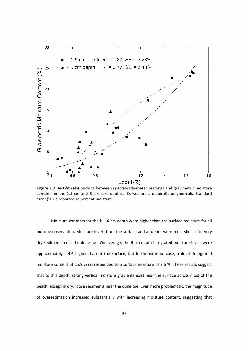
We also fit a spectroradiometer calibration for the 1.5 and 6 cm deep samples, which is

shown in Figure 3.7. While there is still a reasonable relationship between A and gravimetric

moisture content in both cases (R2 ≈ 0.87 for the 1.5 cm deep sample, 0.77 for the 6 cm deep

sample), the standard error is 3.28 and 3.10 % moisture content, respectively, compared to the

0.61 and 1.22 % standard error values from the Theta probe. As expected, these results indicate

that the spectoradiometer is well suited to measure moisture at the beach surface, while it does

not accurately predict moisture conditions integrated over the top few cm of sediment.

Conversely, the Theta probe is well suited to measure moisture content integrated at some

depth, but not well suited to predict moisture content at the surface, which agrees with findings

from Nield et al. (2011).

Despite the above discrepancy, it is apparent that the TDR probe and the

spectroradiometer are both capable of providing a consistent, reasonably accurate indication of

the moisture content of the sediment thickness they are intended to sample. The question

remains as to how well depth-integrated values are representative of the conditions at the

surface.

Comparison of Depth-Integrated Moisture to Surface Moisture

The depth-integrated moisture contents measured with the Theta probe are compared

with the surface moisture measurements from the spectroradiometer in Figure 3.8. It is clear

that there is substantial disagreement between the two. Because the respective instruments

used here produce accurate measures of surface and depth integrated moisture contents, the

scatter in Figure 3.8 can likely be attributed to natural gradients in moisture with depth. It is

readily apparent that depth-integrated moisture contents can differ quite a bit from the surface

contents at the same locations.

37

Figure 3.7 Best-fit relationships between spectroradiometer readings and gravimetric moisture content for the 1.5 cm and 6 cm core depths. Curves are a quadratic polynomials. Standard error (SE) is reported as percent moisture.

Moisture contents for the full 6 cm depth were higher than the surface moisture for all

but one observation. Moisture levels from the surface and at depth were most similar for very

dry sediments near the dune toe. On average, the 6 cm depth-integrated moisture levels were

approximately 4.4% higher than at the surface, but in the extreme case, a depth-integrated

moisture content of 15.9 % corresponded to a surface moisture of 3.6 %. These results suggest

that to this depth, strong vertical moisture gradients exist near the surface across most of the

beach, except in dry, loose sediments near the dune toe. Even more problematic, the magnitude

of overestimation increased substantially with increasing moisture content, suggesting that

38

moisture gradients steepen across the mid beach, possibly because the bottom of the

integrated volume is increasingly more connected via capillary action to the water table as

beach elevation decreases towards the swash zone. For two saturated swash zone samples,

surface moisture predictions from the spectroradiometer exceeded the maximum gravimetric

moisture level possible for beach sands because a thin layer of water was present above the

sediment surface. Thus, these data are not shown, but it can be assumed that surface and

depth-integrated moisture would match for very wet sediments due to vertically ubiquitous

saturation in the swash zone.

For the shallower 1.5 cm sampling depth, the disagreement between the depth-

integrated measurements and the surface measurements is not as large, but is much more

variable. Depth-integrated moisture levels are higher than at the surface by about 2.5% on

average, although moisture contents were higher at the surface in a few instances. The

increased variability in the relationship between surface moisture and depth-integrated

moisture suggests that over this shallower integration depth, near-surface gradients are less

predictable, particularly in the mid beach. At this depth, sediments are likely further detached

from the water table, and as such likely subject to more variability in the magnitude and

direction of gradients. Again, data from two saturated samples are not shown for the same

reasons as above, but the best agreement between the surface moisture and depth-integrated

moisture for this depth occurred with very dry or very wet sediments, which agrees with

intuitive expectations that in very dry or wet regions near the dune toe or swash zone, there will

be less vertical variability in moisture content. There were also several instances on the upper

mid beach, near the dune toe, where the surface was dry, but there was significant moisture at

depth.

39

Figure 3.8 Comparison of depth-integrated moisture measurements from the Theta probe versus surface moisture measurements from the spectroradiometer. Linear best-fit relationships are shown for each probe sampling depth. Depth-integrated measurements generally overestimated moisture at the surface. Depth-integrated moisture content and surface moisture content were similar for very dry or very wet conditions, i.e. at the dune toe and near the swash zone, and most of the departure occurred in the mid beach area.

In all, it is apparent that the use of measurements integrated over even relatively

shallow depths are likely to overestimate actual surface moisture content across much of the

beach surface, particularly in intermediate moisture zones across the mid beach and transport

intensive areas near the dune toe (e.g. where sediments on the surface may be dry, but there is

moisture at depth). Thus, depth-integrated moisture data may not be appropriate to represent

conditions at the air-sediment interface, and could potentially produce misleading experimental

results designed to assess the effects of moisture on aeolian processes. Interestingly, although

40

the magnitude of departure is larger, there appears to be a more predictable relationship

between surface moisture and the 6 cm sampling depth than for the 1.5 cm sampling depth.

According to these data, the larger sampling depth can be used to predict moisture at the

surface to within about 0.7%, while the standard error of prediction for surface moisture from

the 1.5 cm measurements is about 2.8% moisture content.

3.4 Discussion and Conclusions

The goal of this study was to compare depth-integrated moisture measurements to

conditions at the surface. Comparison of surface moisture measurements obtained with a

spectroradiometer with depth-integrated measurements obtained with a Theta probe revealed

that the depth-integrated measurements were higher at the surface of the bed by an average of

2.5% moisture for 1.5 cm deep samples and 4.4% moisture for 6 cm deep samples. There was

enough scatter and variability in the magnitude of overestimation to suggest that the depth-

integrated measurements may not suitably characterize surface moisture levels for studies

focused on aeolian transport, where only the top few layers of grains are usually considered

important. However, the difference between the surface moisture and moisture over depth was

often negligible for areas near and on the dune toe and swash zone, as one might expect. The

largest departures between surface and depth-integrated moisture occurred on the mid beach

area, where there is likely a complex interplay between capillary and atmospheric processes

that determine moisture at the surface. Perhaps most important for aeolian studies was the

overestimation of moisture on the the upper mid beach near the dune toe, where sediments at

the surface were dry but moist to some degree at depth. It was also found that measurements

integrated over increasingly large depths tend to depart from surface moisture content by an

increasingly large amount across the beach surface, as would be expected. There was, however,

41

a more predictable relationship between surface moisture and depth-integrated moisture at

larger depths.

Admittedly, this research is not definitive in terms of the magnitude or direction of near

-surface moisture gradients we could expect under different scenarios (e.g. drying/wetting

cycles), with different grain sizes, or with different inclement conditions, but adds to a very

sparse existing framework with regards to the behavior of moisture near the surface of the

sediment bed. In terms of aeolian transport research, these results imply that previous studies

that employed depth-integrated moisture measurement techniques may have underestimated

the transport-limiting influence of surface moisture. For example, the oft-cited Chepil (1956),

Hotta et al. (1984), Sherman et al. (1998), and Davidson-Arnott et al. (2008) used measurement

depths of 0.64, 0.5, 0.5, and 2.0 cm, respectively. Further, uncertainty regarding ‘true’ surface

moisture seems to be greatest on areas of the beach likely to experience transport, e.g. the

upper mid beach. As moisture is a key control on transport thresholds and rates, much more

work is needed still to investigate the nature of near-surface gradients, especially in terms of

spatial variability across the beach.

An ancillary goal was to briefly evaluate the utility of a hand-held spectroradiometer for

measuring beach surface moisture contents. From a practical standpoint, the spectroradiometer

is somewhat cumbersome to use in the field because of the need to control the device with a

computer and the need to record frequent white reference measurements. Sampling speed is

therefore relatively slow, and it would not be a very practical instrument for repeated moisture

content mapping of large areas, as in McKenna Neuman and Langston (2006), Darke and

McKenna Neuman (2008), Delgado-Fernandez et al. (2009), Darke et al. (2009), Namikas et al.

(2010), Delgado-Fernandez and Davidson-Arnott, 2011, Delgado-Fernandez (2011), or Nield et

al., (2011). However, the device is very well suited to sample smaller numbers of points at

42

regular intervals and it appears to potentially provide a significantly more accurate

characterization of moisture content at the surface than previous non-destructive remote

sensing attempts (McKenna Neuman and Langston, 2003, 2006; Darke and McKenna Neuman,

2008; Dark et al., 2009; Delgado-Fernandez, Davidson-Arnott, and Ollerhead, 2009, Nield and

Wiggs, 2011, Nield et al., 2011).

We admit this assertion is based on a small sampling of calibration points, but when

considered together with the laboratory calibration and the available body of work from the

agricultural and remote sensing fields (e.g., Kano et al., 1985; Slaughter et al., 2001; Lobell and

Asner, 2002; Weidong et al, 2002; Weidong et al., 2003; Mouazen et al., 2007) , the results from

this study suggest that infrared wavelengths can potentially provide improved information

regarding surface moisture content on beaches in comparison to visible wavelengths. An

approach that used infrared filters or sensors with digital photography might prove to be a

useful advance by combining the accuracy from infrared signals with the measurement ease and

spatio-temporal resolution of digital photography. More work is needed to develop accurate,

non-destructive, and rapid techniques to quantify moisture content at the beach sediment

surface.

3.5 References

Analytical Spectral Devices. 2002. FieldSpec® UV/VNIR HandHeld Spectroradiometer User’s Guide. Boulder, CO: ASD Inc. Atherton RJ, Baird AJ, Wiggs GFS. 2001. Inter-tidal dynamics of surface moisture content on a meso-tidal beach. Journal of Coastal Research 17, 482-489. Bauer BO, Davidson-Arnott RGD; Hesp PA; Namikas SL; Ollerhead J, Walker IJ. 2009. Aeolian sediment transport on a beach: Surface moisture, wind fetch, and mean transport. Geomorphology 105, 106-116. Chepil WS. 1956. Influence of Moisture on Erodibility of Soil by Wind. Soil Science Society of America Proceedings 20, 288-292.

43

Darke I, Davidson-Arnott RGD, Ollerhead J. 2009. Measurement of Beach Surface Moisture Using Surface Brightness. Journal of Coastal Research 25, 248-256. Darke I, McKenna Neuman C. 2008. Field study of beach water content as a guide to wind erosion potential. Journal of Coastal Research 24, 1200-1208. Davidson-Arnott RGD, Bauer BO. 2009. Aeolian sediment transport on a beach: Thresholds, intermittency, and high frequency variability. Geomorphology 105, 117-126. Davidson-Arnott RGD, MacQuarrie K,Aagaard T. 2005. The effect of wind gusts, moisture content and fetch length on sand transport on a beach. Geomorphology 68, 115-129. Davidson-Arnott RGD, Yang Y, Ollerhead J, Hesp P.A, and Walker IJ. 2008. The effects of surface moisture on aeolian sediment transport threshold and mass flux on a beach. Earth Surface Processes and Landforms 33, 55-74. Delgado-Fernandez I. 2011. Meso-scale modelling of aeolian sediment input to coastal dunes. Geomorphology 130, 230-243. Delgado-Fernandez I, Davidson-Arnott RGD. 2011. Meso-scale aeolian sediment input to coastal dunes: The nature of aeolian transport events. Geomorphology 126. 117-232. Delgado-Fernandez I, Davidson-Arnottt RGD, Ollerhead J. 2009. Application of a Remote Sensing Technique to the Study of Coastal Dunes. Journal of Coastal Research 25, 1160-1167. Edwards BL, Namikas SL. 2009. Small-scale variability in surface moisture on a fine-grained beach: implications for modeling aeolian transport. Earth Surface Processes and Landforms 34, 1333-1338. Gares PA, Davidson-Arnott RGD, Bauer BO, Sherman DJ, Carter RWG, Jackson DWT, and Nordstrom KF. 1996. Alongshore variations in aeolian sediment transport, Carrick Finn Strand, Ireland. Journal of Coastal Research 12, 673-682. Gaskin GJ, Miller JD. 1996. Measurement of soil water content using a simplified impedance measuring technique. Journal of Agricultural Engineering Research 63, 153-159. Hotta S, Kubota S, Katori S, Horikawa K. 1984. Sand Transport by Wind on a Wet Sand Surface. Proceedings of the 19th Coastal engineering Conference (New York, New York, ASCE), pp. 1263-1281. Huang Q, Akinremi OO, Rajan RS, Bullock R. 2004. Laboratory and field evaluation of five soil water sensors. Canadian Journal of Soil Science 84, 431-438. Jackson NL, Nordstrom KL. 1997. Effects of time-dependent moisture content of surface sediments on aeolian transport rates across a beach, Wildwood, New Jersey, U.S.A. Earth Surface Processes and Landforms 22, 611–621.

44

Kano Y, McClure WF, Skaggs RW. 1985. A Near-Infrared Reflectance Soil-Moisture Meter. Transactions of the ASAE 28, 1852-1855. Kroon A, Hoekstra P. 1990. Eolian Sediment Transport on a Natural Beach. Journal of Coastal Research 6, 367-379. Lobell, DB, Asner, GP. 2002. Moisture effects on soil reflectance. Soil Science Society of America Journal 66, 722-727. McKenna Neuman CL, Langston G. 2003. Spatial analysis of surface moisture content on beaches subject to aeolian transport. Proceedings of the Canadian Coastal Conference (Kingston, Ontario, Canada), pp. 1-10. McKenna Neuman CL, Langston G. 2006. Measurement of water content as a control of particle entrainment by wind. Earth Surface Processes and Landforms, 31, 303-317. Mouazen AM, Maleki MR, De Baerdemaeker J, Ramon H. 2007. On-line measurement of some selected soil properties using a VIS-NIR sensor. Soil & Tillage Research, 93, 13-27. Namikas SL, Edwards BL, Bitton MCA, Booth JL, Zhu Y. 2010. Temporal and spatial variabilities in the surface moisture content of a fine-grained beach. Geomorphology 114, 303-310. Nield JM, Wiggs GF. 2011. The application of terrestrial laser scanning to aeolian saltation cloud measurement and its response to changing surface moisture. Earth Surface Processes and Landforms 36, 273-278. Nield JM, Wiggs GF, Squirrell RS. 2011. Aeolian sand strip mobility and protodune development on a drying beach: examining surface moisture and surface roughness patterns measured by terrestrial laser scanning. Earth Surface Processes and Landforms 36, 513-522. Nordstrom KF, Bauer BO, Davidson-Arnott RGD, Gares PA, Carter RWG, Jackson DWT, Sherman DJ. 1996. Offshore aeolian transport across a beach, Carrick Finn Strand, Ireland. Journal of Coastal Research 12, 664-672. Oblinger A, Anthony EJ. 2008. Surface moisture variations on a multibarred macrotidal beach: Implications for aeolian sand transport. Journal of Coastal Research 24, 1194-1199. Sarre RD. 1988. Evaluation of Aeolian sand transport equations using intertidal zone measurements, Saunton Sands, England. Sedimentology 35, 671-679. Schmutz PP, Namikas SL. 2011. Utility of the Delta-T Theta Probe for obtaining surface moisture measurements from beaches. Journal of Coastal Research 27, 478-484. Sherman DJ, Jackson DWT, Namikas SL, Wang JK. 1998. Wind-blown sand on beaches: an evaluation of models. Geomorphology 22, 113-133. Slaughter DC, Pelletier MG, Upadhyaya SK. 2001. Sensing soil moisture using NIR spectroscopy. Applied Engineering in Agriculture 17, 241-247.

45

Tsegaye TD, Tadesse W, Coleman TL, Jackson TJ, Tewolde H. 2004. Calibration and modification of impedance probe for near surface soil moisture measurements. Canadian Journal of Soil Science 84, 237-243. Turner IL. 1993. The Total Water Content of Sandy Beaches. In: Short, A.D. (ed.) Beach and Surf Zone Morphodynamics. Journal of Coastal Research Special Issue 15, pp. 11-26. Weidong L, Baret F, Xingfa G, Qingxi T, Lanfen Z, Bing Z. 2002. Relating soil surface moisture to reflectance. Remote Sensing of Environment 81, 238-246. Weidong L, Baret F, Xingfa G, Bing Z, Qingxi T, Lanfen Z. 2003. Evaluation of methods for soil surface moisture estimation from reflectance data. International Journal of Remote Sensing 24, 2069-2083. Wiggs GFS, Baird AJ, Atherton RJ. 2004. The dynamic effects of moisture on the entrainment and transport of sand by wind. Geomorphology 59, 13-30. Yang YQ, Davidson-Arnott RGD. 2005. Rapid measurement of surface moisture content on a beach. Journal of Coastal Research 21, 447-452.

46

4. SIMPLE INFRARED TECHNIQUES FOR MEASURING BEACH SURFACE MOISTURE3

4.1 Introduction

It is well known that surficial moisture exerts significant control on aeolian transport

processes. Identification of spatiotemporal variations in surficial moisture is a critical need in

coastal aeolian research, and contemporary field studies of aeolian processes often incorporate

some form of surface moisture measurement (e.g. Davidson-Arnott et al., 2008; Bauer and

Davidson-Arnott, 2009; Davidson-Arnott, et al., 2009; Nield et al., 2011). Conceptually, the role

of moisture is simple: cohesion caused by inter-granular water adds additional resistance to

motion (beyond inertial forces), which manifests as an increase in entrainment threshold and a

decrease in the rate of mass transport (see Hotta et al. (1984), Namikas and Sherman (1995),

and Cornelis and Gabriels (2003) for detailed reviews). However, the degree to which moisture

influences transport processes under field conditions is still largely unknown.

Numerous models that describe the influence of surface moisture on aeolian transport

in either empirical or theoretical terms have been proposed (e.g. Akiba, 1933; Chepil, 1956;

Belly, 1964; Kawata and Tsuchiya, 1976; Azizov, 1977; Horiwaka et al., 1982; Hotta et al., 1984;

Sarre, 1988; McKenna Neuman and Nickling, 1989; Gregory and Darwish, 1990; Shao et al.,

1996; Cornelis et al. 2004a, 2004b, 2004c). However, a key limitation substantively restricts the

application of such models to field situations. Essentially, an inability to quantify surface

moisture content with appropriate precision and with sufficient spatial and temporal resolution

leading up to and during transport events has seriously limited progress in the understanding of

how surface moisture influences thresholds and mass transport rates and affects transport

dynamics in the complex conditions found on a natural beach. Consequently, the pursuit of

improved field measurement techniques has been an area of focus in the literature, and a

3 Reproduced with permission from Earth Surface Processes and Landforms. See APPENDIX III

47

number of technical advances have been made in recent years (e.g. Atherton et al., 2001; Yang

and Davidson-Arnott, 2005; McKenna Neuman and Langston, 2003, 2006; Darke and McKenna

Neuman, 2008; Darke, et al., 2009; Delgado-Fernandez et al., 2009, Nield and Wiggs, 2011).

There is still need for improvement, however, in our ability to precisely, rapidly and

nondestructively measure moisture where it is most significant for aeolian processes – the

uppermost few layers of grains. This paper examines the potential of a new approach to the

problem, the use of handheld infrared remote sensing, and presents results from field tests

designed to assess the suitability of an inexpensive narrow-band infrared radiometer as a tool to

measure beach surface moisture and a comparison with a standard commercial

spectroradiometer.

4.2 Background

A variety of methods have been used to measure surface moisture on beaches,

including collecting sediment scrapings from the surface (e.g., Sarre, 1988, Kroon and Hoekstra,

1990; Gares et al., 1996; Nordstrom et al., 1996; Jackson and Nordstrom, 1997, Sherman et al.,

1998; Wiggs et al., 2004; Davidson-Arnott et al., 2005), commercial soil moisture probes (Svasek

and Terwindt, 1974, Atherton et al., 2001; Wiggs et al., 2004; Yang and Davidson-Arnott, 2005;

Davidson-Arnott et al., 2008; Oblinger and Anthony, 2008; Bauer et al., 2009; Davidson-Arnott

and Bauer, 2009; Edwards and Namikas, 2009; Namikas et al., 2010), and remote sensing

techniques such as digital photography (McKenna Neuman and Langston, 2003, 2006; Darke and

McKenna Neuman, 2008; Darke et al., 2009; Delgado-Fernandez et al., 2009, Delgado-

Fernandez, 2011) and a terrestrial laser scanner (Nield and Wiggs., 2011, Nield et al., 2011). Each

approach has specific advantages and shortcomings with regard to accuracy and resolution

(spatial and temporal). For example, surface scraping is generally considered to provide the

48

most accurate measurement, but the collection process effectively destroys the surface and

thereby complicates repeated sampling of the same location (which is needed to document

temporal change in moisture content). Many commercial probes can be used to document

temporal change with high resolution, but they generally sample a volume that is large enough

to make their application to a very thin surface layer problematic.

In general, remote sensing approaches hold great promise for aeolian process studies

because they overcome two fundamental problems associated with surface scrapings and

probes: 1) the integrity of the surface is preserved undisturbed; and 2) only the top few layers of

grains are sampled. Recent studies have demonstrated the potential utility of remote sensing

approaches to characterize meso-scale spatio-temporal patterns in surficial moisture conditions

(McKenna Neuman and Langston, 2003, 2006; Darke and McKenna Neuman, 2008; Darke et al.,

2009; Delgado-Fernandez et al., 2009; Delgado-Fernandez, 2011; Nield and Wiggs, 2011; Nield

et al., 2011). However, the highest level of accuracy reported from brightness measurements to

date is a standard error of 3% to 4% (Darke et al., 2009), and in many cases, the scatter in

calibrations exceeds approximately 10% moisture content for a given surface brightness

(McKenna Neuman and Langston, 2003, 2006; Darke and McKenna Neuman, 2008; Darke,

Davidson-Arnott, and Ollerhead, 2009; Delgado-Fernandez, Davidson-Arnott, and Ollerhead,

2009), which would introduce considerable uncertainty in transport rate modeling. Terrestrial

laser scanning appears to hold great promise for the future, but it is currently a cutting edge

technology that is potentially expensive and produces large amounts of data that require a great

deal of post processing (Nield and Wiggs, 2011, Nield et al., 2011). Further, scatter in the

calibration of the laser scanner appears large above low moisture contents, and appears to

increase until moisture above levels of 7 or 8% cannot be predicted with certainty.

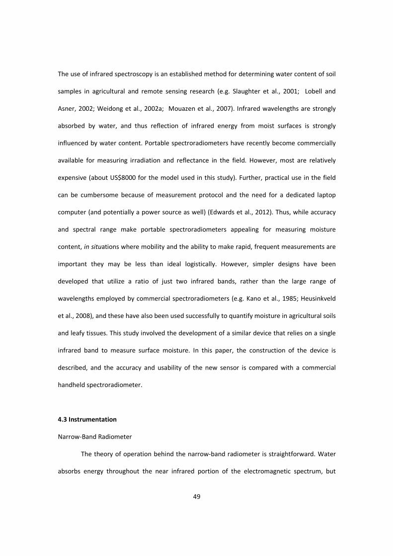
49

The use of infrared spectroscopy is an established method for determining water content of soil

samples in agricultural and remote sensing research (e.g. Slaughter et al., 2001; Lobell and

Asner, 2002; Weidong et al., 2002a; Mouazen et al., 2007). Infrared wavelengths are strongly

absorbed by water, and thus reflection of infrared energy from moist surfaces is strongly

influenced by water content. Portable spectroradiometers have recently become commercially

available for measuring irradiation and reflectance in the field. However, most are relatively

expensive (about US$8000 for the model used in this study). Further, practical use in the field

can be cumbersome because of measurement protocol and the need for a dedicated laptop

computer (and potentially a power source as well) (Edwards et al., 2012). Thus, while accuracy

and spectral range make portable spectroradiometers appealing for measuring moisture

content, in situations where mobility and the ability to make rapid, frequent measurements are

important they may be less than ideal logistically. However, simpler designs have been

developed that utilize a ratio of just two infrared bands, rather than the large range of

wavelengths employed by commercial spectroradiometers (e.g. Kano et al., 1985; Heusinkveld

et al., 2008), and these have also been used successfully to quantify moisture in agricultural soils

and leafy tissues. This study involved the development of a similar device that relies on a single

infrared band to measure surface moisture. In this paper, the construction of the device is

described, and the accuracy and usability of the new sensor is compared with a commercial

handheld spectroradiometer.

4.3 Instrumentation

Narrow-Band Radiometer

The theory of operation behind the narrow-band radiometer is straightforward. Water

absorbs energy throughout the near infrared portion of the electromagnetic spectrum, but

50

certain narrow bands of wavelengths are absorbed much more strongly. These absorption peaks

occur at approximately 970 nm, 1200 nm, 1450 nm, and 1940 nm. The absorption band at 1940

nm is by far the strongest, and at this wavelength wetter sands should absorb much higher

amounts of energy than dry sands. Thus, if a constant infrared energy level is applied to the

beach surface, energy in this band received at a sensor should be inversely related to the water

content at the surface.

The major components of the narrow-band radiometer (NBR) consist of a light source to

generate infrared energy and a photodetector that is mounted behind a narrow bandpass filter

that only allows a small band centered around 1940 nm to pass. The instrument housing was

constructed of PVC pipe, and consisted of a light chamber and the main detection chamber

(Figure 1). The photodetector and light were mounted on solid core aluminum disks (heatsinks)

which fit inside the PVC joints and basic circuitry was housed above. The sensing end of the

device was capped with a quartz glass disk to prevent moisture or other contaminants from

getting inside. A GU-5.3 socket MR-16 50 watt halogen bulb was used as the light source and

was mounted in a 12/24 Volt ceramic socket which was mounted to the heatsink in the light

chamber. The photodetector was a ThorLabs model FGA20 InGAas photodiode in a TO-18

package (3 leads: anode, cathode, case ground). This particular sensor has a range of about 1200

to 2600 nm, with peak response from about 1900 to 2300 nm. The bandpass filter was the same

diameter of the sensor package and had a 40 nm bandwidth centered on 1940 nm. A reverse

bias of approximately 1.6 Volts was applied to the photodiode via a voltage regulator powered

by a nine volt battery, and output photocurrent was converted to voltage with a 1 kOhm load

resistor. The light source was powered using a 12 Volt 7 amp-hour battery. Total cost of

components was about US$800.

51

Practical operation of the device is also straightforward. In this configuration, as the

amount of moisture in a sample increases, the amount of energy that strikes the detector and

thus the current generated and resulting voltage output decrease. Output voltage was

measured at 1 Hz using a portable external data logger that also recorded time and ambient

temperature. The photodetector continuously outputs a signal, but for a sample measurement,

the light can be switched on a few seconds before to record a base level voltage and to mark

each measurement in the logged data sequence. Next, the instrument is held just above the

sample area for a few seconds to record a measurement voltage. Finally, the instrument is

removed from the sample and the light is left on for a few seconds more and then switched off.

Each measurement takes about 10 seconds to make. For the tests conducted in this study, the

light was left on for the duration of each because they were conducted over a very short period

of time.

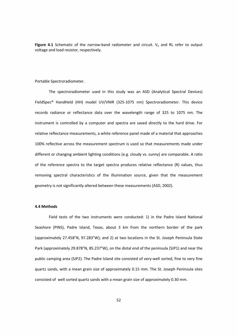
52

Figure 4.1 Schematic of the narrow-band radiometer and circuit. Vo and RL refer to output voltage and load resistor, respectively.

Portable Spectroradiometer.

The spectroradiometer used in this study was an ASD (Analytical Spectral Devices)

FieldSpec® HandHeld (HH) model UV/VNIR (325-1075 nm) Spectroradiometer. This device

records radiance or reflectance data over the wavelength range of 325 to 1075 nm. The

instrument is controlled by a computer and spectra are saved directly to the hard drive. For

relative reflectance measurements, a white reference panel made of a material that approaches

100% reflective across the measurement spectrum is used so that measurements made under

different or changing ambient lighting conditions (e.g. cloudy vs. sunny) are comparable. A ratio

of the reference spectra to the target spectra produces relative reflectance (R) values, thus

removing spectral characteristics of the illumination source, given that the measurement

geometry is not significantly altered between these measurements (ASD, 2002).

4.4 Methods

Field tests of the two instruments were conducted: 1) in the Padre Island National

Seashore (PINS), Padre Island, Texas, about 3 km from the northern border of the park

(approximately 27.458°N, 97.283°W); and 2) at two locations in the St. Joseph Peninsula State

Park (approximately 29.878°N, 85.237°W), on the distal end of the peninsula (SJP1) and near the

public camping area (SJP2). The Padre Island site consisted of very-well sorted, fine to very fine

quartz sands, with a mean grain size of approximately 0.15 mm. The St. Joseph Peninsula sites

consisted of well sorted quartz sands with a mean grain size of approximately 0.30 mm.

53

One test of the NBR was conducted at each of the three sites. After each measurement

was taken, a 1.5 mm thick layer of the measured sediment was collected (roughly 5 grains deep

at SJP and 10 grains deep at PINS). The samples were sealed in plastic bags and initial weights

were recorded the day of extraction. Moisture contents were subsequently determined in the

laboratory using standard gravimetric techniques. Ambient air temperature was also recorded

in conjunction with surface moisture sensor measurements.

Two field tests of the spectroradiometer were conducted for comparison, one at SJB1

and one at the PINS site (Edwards et al., 2012). For each measurement, a white reference

measurement was conducted, and 6 spectra were recorded immediately after. Relative

reflectance at 970 nm (a weak water absorption band) was averaged for each sample.

Gravimetric moisture contents of the sediments were determined in the same manner as above.

4.5 Results

Narrow-band radiometer

Figure 4.2 shows an example of instrument output from one of the field calibration tests

(SJP1). Each of the peaks in the series represents one of the target measurement points. Despite

moisture level, reflection of energy from the sand surface is higher than base level output for all

possible values. However, moister sands absorb more energy, and the measurement peak is

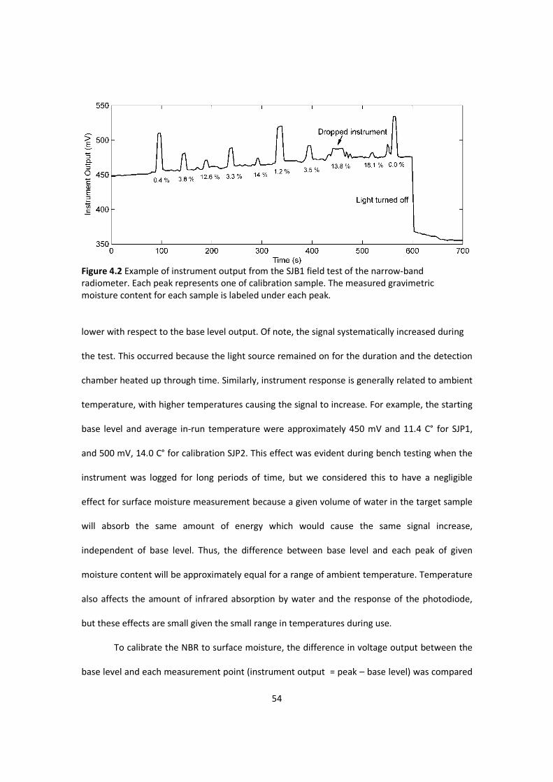
54

Figure 4.2 Example of instrument output from the SJB1 field test of the narrow-band radiometer. Each peak represents one of calibration sample. The measured gravimetric moisture content for each sample is labeled under each peak.

lower with respect to the base level output. Of note, the signal systematically increased during

the test. This occurred because the light source remained on for the duration and the detection

chamber heated up through time. Similarly, instrument response is generally related to ambient

temperature, with higher temperatures causing the signal to increase. For example, the starting

base level and average in-run temperature were approximately 450 mV and 11.4 C° for SJP1,

and 500 mV, 14.0 C° for calibration SJP2. This effect was evident during bench testing when the

instrument was logged for long periods of time, but we considered this to have a negligible

effect for surface moisture measurement because a given volume of water in the target sample

will absorb the same amount of energy which would cause the same signal increase,

independent of base level. Thus, the difference between base level and each peak of given

moisture content will be approximately equal for a range of ambient temperature. Temperature

also affects the amount of infrared absorption by water and the response of the photodiode,

but these effects are small given the small range in temperatures during use.

To calibrate the NBR to surface moisture, the difference in voltage output between the

base level and each measurement point (instrument output = peak – base level) was compared

55

to moisture content from the surface scraping. Figure 4.3 shows the calibration curves for both

SJP field tests. The dry sediment instrument output was about 60 mV. For each test, output

decreased exponentially as moisture content increased. Independently, the calibrations have R2

values of 0.99 and standard error values of 0.4 and 0.6 % moisture content, respectively. It is

encouraging that near-identical results are obtained from two different locations on two

different days. The agreement between the calibrations is evident in the combined calibration

curve (R2 = 0.98, standard error = 1.0 % moisture). There was a slight difference in grain size

between the two locations (approximately 12 km apart), and this likely contributed to the small

difference in calibrations.

Figure 4.4 shows the results from the field calibration at the PINS site. Instrument

response is just as strongly correlated to moisture content (R2 value of 0.99). Accuracy is lower

than for either of the SJB tests considered independently, but on par with the combined results

(standard error = 1.0 % moisture content). Instrument output on the whole was larger for these

sands, which indicates that more infrared energy is reflected as a whole, but had a smaller full-

scale range, varying by only about 25 mV as opposed to almost 60 mV for the SJB sites.

Spectroradiometer

Figure 4.5 shows an example of spectra measured for a range of moisture contents from

the SJB1 field test recorded by the spectroradiometer. Of note, the signal becomes saturated (R

= 1.0) to varying degrees in the visible wavelengths for this particular sediment. Also, trends in R

with respect to wavelength are generally persistent for different moisture levels. There is a large

amount of variability for each moisture level in the ultraviolet and visible portions of the

spectrum, but the spectra become much smoother in the infrared. In this range, the maximum

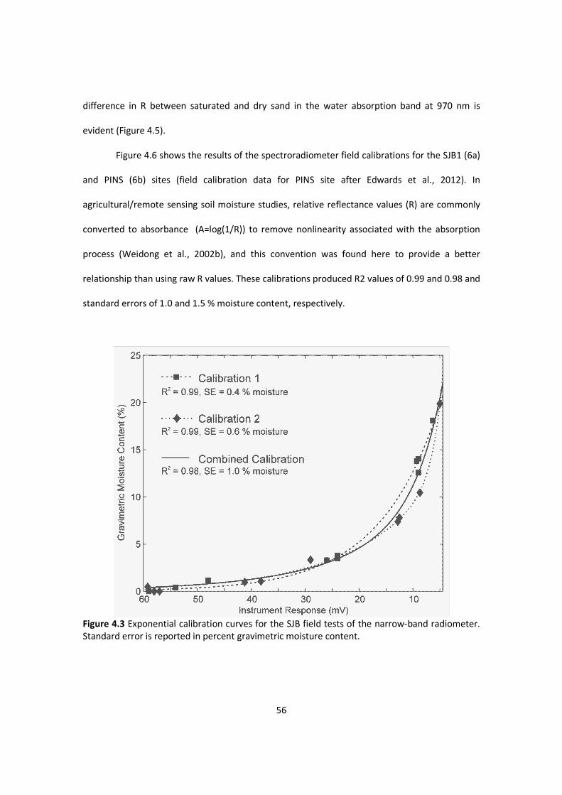
56

difference in R between saturated and dry sand in the water absorption band at 970 nm is

evident (Figure 4.5).

Figure 4.6 shows the results of the spectroradiometer field calibrations for the SJB1 (6a)

and PINS (6b) sites (field calibration data for PINS site after Edwards et al., 2012). In

agricultural/remote sensing soil moisture studies, relative reflectance values (R) are commonly

converted to absorbance (A=log(1/R)) to remove nonlinearity associated with the absorption

process (Weidong et al., 2002b), and this convention was found here to provide a better

relationship than using raw R values. These calibrations produced R2 values of 0.99 and 0.98 and

standard errors of 1.0 and 1.5 % moisture content, respectively.

Figure 4.3 Exponential calibration curves for the SJB field tests of the narrow-band radiometer. Standard error is reported in percent gravimetric moisture content.

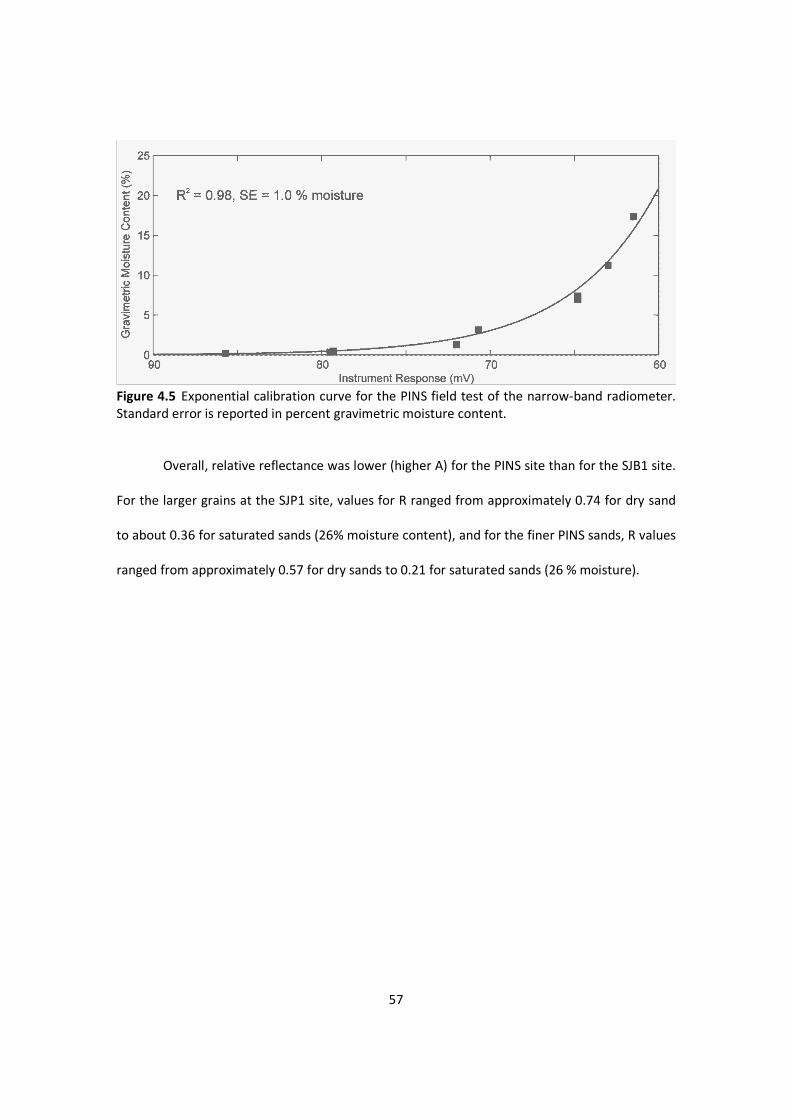
57

Figure 4.5 Exponential calibration curve for the PINS field test of the narrow-band radiometer. Standard error is reported in percent gravimetric moisture content.

Overall, relative reflectance was lower (higher A) for the PINS site than for the SJB1 site.

For the larger grains at the SJP1 site, values for R ranged from approximately 0.74 for dry sand

to about 0.36 for saturated sands (26% moisture content), and for the finer PINS sands, R values

ranged from approximately 0.57 for dry sands to 0.21 for saturated sands (26 % moisture).

Figure 4.5 Selected relative reflectance (value of 1 represents saturation of the signal with respect to the white reference measurement. The water absorption band at 970 nm is marked to highlight theNIR range of the spectra in R

4.6 Discussion and Conclusions

The full-scale range of instrument response varied by site for both instruments, in each

case being smaller for the PINS site. This s

58

Selected relative reflectance (R) spectra from the SJB1 spectroradiometer field test. A value of 1 represents saturation of the signal with respect to the white reference measurement. The water absorption band at 970 nm is marked to highlight the maximum difference over the

R for different moisture levels.

4.6 Discussion and Conclusions

scale range of instrument response varied by site for both instruments, in each

case being smaller for the PINS site. This suggests that the instruments do not ‘see’ water as well

) spectra from the SJB1 spectroradiometer field test. A value of 1 represents saturation of the signal with respect to the white reference measurement.

maximum difference over the

scale range of instrument response varied by site for both instruments, in each

uggests that the instruments do not ‘see’ water as well

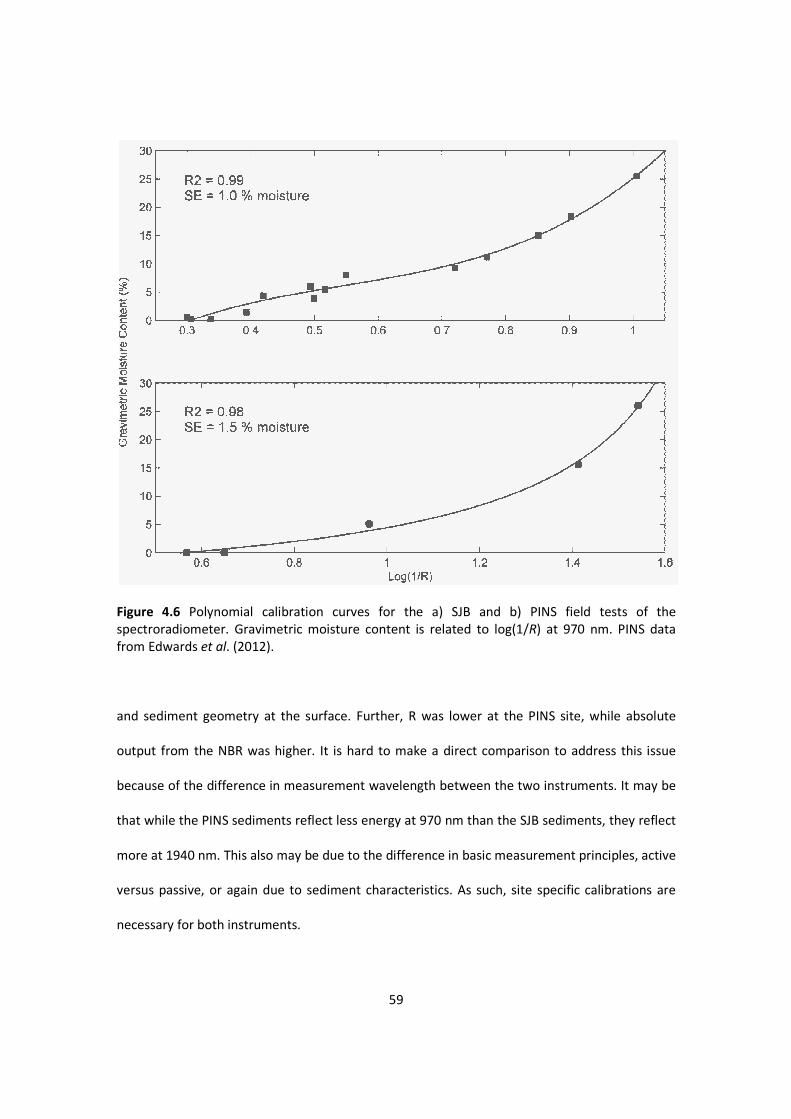
Figure 4.6 Polynomial calibration curves for the a) SJB and b) PINS field tests of the spectroradiometer. Gravimetric moisture content is related to log(1/from Edwards et al. (2012).

and sediment geometry at the surface. Further, R was lower at the PINS site, while absolute

output from the NBR was higher. It is hard to make a direct comparison to address this issue

because of the difference in measurement wavelength betwe

that while the PINS sediments reflect less energy at 970 nm than the SJB sediments, they reflect

more at 1940 nm. This also may be due to the difference in basic measurement principles, active

versus passive, or again due

necessary for both instruments.

59

Polynomial calibration curves for the a) SJB and b) PINS field tests of the spectroradiometer. Gravimetric moisture content is related to log(1/R) at 970 nm. PINS data

and sediment geometry at the surface. Further, R was lower at the PINS site, while absolute

output from the NBR was higher. It is hard to make a direct comparison to address this issue

because of the difference in measurement wavelength between the two instruments. It may be

that while the PINS sediments reflect less energy at 970 nm than the SJB sediments, they reflect

more at 1940 nm. This also may be due to the difference in basic measurement principles, active

versus passive, or again due to sediment characteristics. As such, site specific calibrations are

necessary for both instruments.

Polynomial calibration curves for the a) SJB and b) PINS field tests of the ) at 970 nm. PINS data

and sediment geometry at the surface. Further, R was lower at the PINS site, while absolute

output from the NBR was higher. It is hard to make a direct comparison to address this issue

en the two instruments. It may be

that while the PINS sediments reflect less energy at 970 nm than the SJB sediments, they reflect

more at 1940 nm. This also may be due to the difference in basic measurement principles, active

to sediment characteristics. As such, site specific calibrations are

60

Both of these techniques provide suitable means and high levels of accuracy (< 1.5%

moisture in all cases) for determination of surface moisture content on beaches. For the SJP

sites, the NBR outperformed the spectroradiometer in the individual tests, but when the results

were combined, accuracy was nearly identical. The NBR also outperformed the

spectroradiometer at the PINS site, but this is potentially due to the relatively small number of

calibration samples for the latter (two samples were compromised during transport).

The difference in spectral variability across the visible wavelengths and across infrared

wavelengths revealed in Figure 5 is intriguing. Recent studies using brightness values derived

from digital photography of visible wavelengths have shown promise for collecting spatially and

temporally extensive measurements of beach surface moisture, but calibration results have

generally shown fairly large standard errors (McKenna Neuman and Langston, 2003, 2006;

Darke and McKenna Neuman, 2008; Darke et al., 2009; Delgado-Fernandez et al., 2009). These

results suggest that this methodology could potentially be improved by restricting data

collection to infrared wavelengths.

In terms of practical usability, both instruments are reasonable for conducting point

measurements of moisture at the sediment surface. Measurement protocol and data processing

are simple for both, and both produce accurate results. However, measurement time for the

NBR is much shorter (≈ 10 s) than for the spectroradiometer (≈ 60 s). Also, because the NBR has

an on-board light source and shields ambient radiation, there is no need to conduct reference

measurements, which should be done for every measurement with the spectroradiometer.

Further, because of greater portability, the NBR is easier to use when measuring large numbers

of points.

For aeolian process studies, the measurement approach described in this paper may

best be suited to smaller-scale studies where measurements are conducted at limited locations.

61

Although both instruments are remote sensing instruments, they are handheld, and require the

researcher to be near the measurement point. This could potentially prove disadvantageous in

meso-scale studies where it might require the researcher to traverse a larger study area during

transport events, which could interfere with other measurements. However, for micro-scale

studies, these technologies are portable, and provide accurate measurements of the top few

layers of grains of the sediment bed. Further, accurate point measurements are useful for

studies of the behavior of beach hydrology and surface moisture, independent of transport

events.

Overall, optical infrared methods seem well suited to conduct measurements of beach

surface moisture. For aeolian process studies, accurate measurements of moisture restricted to

the top few layers of grains are desirable, and both of the instruments tested here meet those

criteria. Further, the NBR performed equally as well (or slightly better than) the

spectroradiometer, and is significantly less expensive. More work is needed to refine the

application of these methodologies, but the results of this study indicate this is a promising

avenue for improving the measurement of beach surface moisture.

4.7 References

Akiba M. 1933. Relation between moisture content in sand and the critical wind velocity when sand begins to move. Journal of Agricultural Engineers Society Japan 5, 157-174. Analytical Spectral Devices. 2002. FieldSpec® UV/VNIR HandHeld Spectroradiometer User’s Guide. ASD Inc, Boulder, CO. Atherton RJ, Baird AJ, Wiggs GFS. 2001. Inter-tidal dynamics of surface moisture content on a meso-tidal beach. Journal of Coastal Research 17, 482-489. Azizov A. 1977. Influence of soil moisture in the resistance of soil to wind erosion. Soviet Soil Science 1, 105-108.

62

Bauer BO, Davidson-Arnott RGD, Hesp PA, Namikas SL, Ollerhead J, Walker IJ. 2009. Aeolian sediment transport on a beach, Surface moisture, wind fetch, and mean transport. Geomorphology 105, 106-116. Belly P-Y. 1964. Sand Movement by Wind. Technical Memorandum 1, U.S. Army Corps of Eng CERC, 38p. Chepil WS. 1956. Influence of moisture on erodibility of soil by wind. Soil Science Society of America Proceedings 20, 288–292. Cornelis WM, Gabriels D. 2003. The effect of surface moisture on the entrainment of dune sand by wind, an evaluation of selected models. Sedimentology 50, 771-790. Cornelis WM, Gabriels D, Hartmann R. 2004. A Conceptual Model to Predict the Deflation Threshold Shear Velocity as Affected by Near-Surface Soil Water, I. Theory. Soil Science Society of America Journal 68, 1154-1161. Cornelis WM, Gabriels D, Hartmann R. 2004. A Conceptual Model to Predict the Deflation Threshold Shear Velocity as Affected by Near-Surface Soil Water, II. Calibration and Verification. Soil Science Society of America Journal 68, 1162-1168. Cornelis WM, Gabriels D, Hartmann R. 2004. A parameterization for the threshold shear velocity to initiate deflation of dry and wet sediment. Geomorphology 59, 43–51. Darke I, Davidson-Arnott RGD, Ollerhead J. 2009. Measurement of Beach Surface Moisture Using Surface Brightness. Journal of Coastal Research 25, 248-256. Darke I, Neuman CM. 2008. Field study of beach water content as a guide to wind erosion potential. Journal of Coastal Research 24, 1200-1208. Davidson-Arnott RGD, Bauer BO. 2009. Aeolian sediment transport on a beach, Thresholds, intermittency, and high frequency variability. Geomorphology 105, 117-126. Davidson-Arnott RGD, MacQuarrie K, Aagaard T. 2005. The effect of wind gusts, moisture content and fetch length on sand transport on a beach. Geomorphology 68, 115-129. Davidson-Arnott RGD, Yang Y, Ollerhead J, Hesp PA, Walker IJ. 2008. The effects of surface moisture on aeolian sediment transport threshold and mass flux on a beach. Earth Surface Processes and Landforms 33, 55-74. Delgado-Fernandez I, Davidson-Arnottt RGD, Ollerhead J. 2009. Application of a Remote Sensing Technique to the Study of Coastal Dunes. Journal of Coastal Research 25, 1160-1167. Delgado-Fernandez I. 2011. Meso-scale modelling of aeolian sediment input to coastal dunes. Geomorphology 130, 230-243.

63

Edwards BL, Namikas SL. 2009. Small-scale variability in surface moisture on a fine-grained beach, implications for modeling aeolian transport. Earth Surface Processes and Landforms 34, 1333-1338. Edwards BL, Schmutz PP, Namikas SL. 2012. Comparison of surface moisture measurements to depth-integrated moisture measurements on a fine-grained beach. Journal of Coastal Research. DOI, 10.2112/JCOASTRES-D-12-00008.1 Gares PA, Davidson-Arnott RGD, Bauer BO, Sherman DJ, Carter RWG, Jackson DWT, Nordstrom KF. 1996. Alongshore variations in aeolian transport, Carrick Finn Strand, Republic of Ireland. Journal of Coastal Research 12, 673-682. Gregory JM, Darwish MM. 1990. Threshold friction velocity prediction considering water content. ASAE Paper No. 902562. American Society of Agricultural Engineering, St Joseph; 16 pp. Heusinkveld BG, Berkowicz SM, Jacobs AFG, Hillen W, Holtslag AAM. 2008. A new remote optical wetness sensor and its applications. Agricultural and Forest Meteorology 148, 580-591. Hotta S, Kubota S, Katori S, Horikawa K. 1984. Sand transport by wind on a wet sand surface. In Proceedings of the 19th International Coastal Engineering Conference, Houston, Texas. American Society of Civil Engineers, New York; 1265–1281. Jackson NL, Nordstrom KL. 1997. Effects of time-dependent moisture content of surface sediments on aeolian transport rates across a beach, Wildwood, New Jersey, U.S.A. Earth Surface Processes and Landforms 22, 611–621. Kano Y, McClure WF, Skaggs RW. 1985. A Near-Infrared Reflectance Soil-Moisture Meter. Transactions of the ASAE 28,1852-1855. Kawata Y, Tsuchiya Y. 1976. Influence of water content on the threshold of sand movement and the rate of sand transport in blown sand. Proceedings of the Japanese Society of Civil Engineering 249, 195-100. Kroon A, Hoekstra P, 1990. Eolian Sediment Transport on a Natural Beach. Journal of Coastal Research 6, 367-379. Lobell DB, Asner GP. 2002 Moisture effects on soil reflectance. Soil Science Society of America Journal 66, 722-727. McKenna Neuman CL, Nickling WG. 1989. A theoretical and wind tunnel investigation of the effect of capillary water on the entrainment of sediment by wind. Canadian Journal of Soil Science 69, 79-96. McKenna Neuman CL, Langston G. 2003. Spatial analysis of surface moisture content on beaches subject to aeolian transport. In Proceedings of the Canadian Coastal Conference, Kingston. Ontario. 1-10.

64

McKenna Neuman CL, Langston G. 2006. Measurement of water content as a control of particle entrainment by wind. Earth Surface Processes and Landforms 31, 303-317. Mouazen AM, Maleki MR, De Baerdemaeker J, Ramon H. 2007. On-line measurement of some selected soil properties using a VIS-NIR sensor. Soil & Tillage Research 93, 13-27. Namikas SL, Edwards BL, Bitton MCA, Booth JL, Zhu Y. 2010. Temporal and spatial variabilities in the surface moisture content of a fine-grained beach. Geomorphology 114, 303-310. Nield, JM, Wiggs GF. 2011. The application of terrestrial laser scanning to aeolian saltation cloud measurement and its response to changing surface moisture. Earth Surface Processes and Landforms 36, 273-278. Nield J M, Wiggs GF, Squirrell RS. 2011. Aeolian sand strip mobility and protodune development on a drying beach, examining surface moisture and surface roughness patterns measured by terrestrial laser scanning. Earth Surface Processes and Landforms 36, 513-522. Nordstrom KF, Bauer BO, Davidson-Arnott RGD, Gares PA, Carter RWG, Jackson DWT, Sherman DJ. 1996. Offshore aeolian transport across a beach, Carrick Finn Strand, Ireland. Journal of Coastal Research 12, 664-672. Oblinger A, Anthony EJ. 2008. Surface moisture variations on a multibarred macrotidal beach, Implications for aeolian sand transport. Journal of Coastal Research 24, 1194-1199. Sarre RD. 1988. Evaluation of Aeolian sand transport equations using intertidal zone measurements, Saunton Sands, England. Sedimentology 35, 671-679. Schmutz PP, Namikas SL. 2011. Utility of the Delta-T Theta Probe for obtaining surface moisture measurements from beaches. Journal of Coastal Research 27, 478-484. Shao Y, Raupach MR, Leys JF. 1996. A model for predicting aeolian sand drift and dust entrainment on scales from paddock to region. Australian Journal of Soil Research 34, 309-342. Sherman DJ, Jackson DWT, Namikas SL, Wang J. 1997. Wind-blown sand on beaches, an evaluation of models. Geomorphology 22, 113-133. Slaughter DC, Pelletier MG, Upadhyaya SK. 2001. Sensing soil moisture using NIR spectroscopy. Applied Engineering in Agriculture 17, 241-247. Svasek JN, Terwindt JHJ. 1974. Measurements of sand transport by wind on a natural beach. Sedimentology 21, 311-322. Weidong L, Baret F, Xingfa G, Bing Z, Qingxi T, Lanfen Z. 2002. Evaluation of methods for soil surface moisture estimation from reflectance data. International Journal of Remote Sensing 24, 2069-2083 Weidong L, Baret F, Xingfa G, Qingxi T, Lanfen Z, Bing Z. 2002. Relating soil surface moisture to reflectance. Remote Sensing of Environment 81, 238-246.

65

Wiggs CFS, Baird AJ, Atherton RJ. 2004. The dynamic effects of moisture on the entrainment and transport of sand by wind. Geomorphology 59, 13-30. Yang Y, Davidson-Arnott RGD. 2005. Rapid measurement of surface moisture content on a beach. Journal of Coastal Research 21, 447-452.

66

5. PREDICTING THRESHOLD SHEAR VELOCITY FOR INITATION OF AEOLIAN TRANSPORT OF

QUARTZ SANDS AS A FUNCTION OF MASS AND GRAIN SIZE-RANGE

5. 1 Introduction

Collectively, models of threshold shear velocity for the initiation of aeolian transport

generate a wide range of predictions. In addition, many predictions differ significantly from

experimental observations of the threshold of motion for quartz sands under terrestrial

conditions (normal ranges of air pressure), particularly for larger sized grains. Thus, a basis for

confident prediction of transport thresholds is not currently available, and determining whether

a given wind event will generate transport – particularly in the frequent case of low energy wind

conditions, where shear velocity is near threshold – is uncertain at best. Further, many mass flux

models are at least in part a function of threshold shear velocity, and the lack of confidence

regarding threshold predictions is a possible source of significant error in transport modeling.

Thus, uncertainty regarding threshold conditions undermines efforts to model systems at meso-

to regional scales, both in terms of numbers of transport events and total mass flux (Sherman et

al., 2011).

This paper presents a re-analysis of previously published experimental observations of

transport thresholds. It demonstrates that threshold shear velocity is linearly proportional to the

square root of the mass of a representative grain, where the representative grain is defined as

having the diameter of the mean grain size determined from the distribution of grain mass,

rather than from the distribution of diameters. Based on available data, this linear relationship

provides a reliable prediction of threshold conditions for quartz sand grains, and given that the

data were drawn from studies that spanned a range of experimental conditions and techniques

across nearly 8 decades, is thought to provide a much more reliable approximation of threshold

conditions.

67

5.2 Models and Observations of Aeolian Transport Thresholds

For the case of dry grains where interparticle cohesion is ignored (Gregory and Darwish

1990), most models of aeolian transport thresholds relate threshold shear velocity (u*t (m/s)) to

the square root of mean grain diameter (d50 (mm)), following Bagnold’s (1936) approach:

�∗� = ������ �� � (5.1)

where ρs and ρa are the density of sediment and air (g/cm3 and kg/m3), respectively, g is

acceleration due to gravity (m/s2) and A is a dimensionless coefficient. Equation 5.1 is based on

the balance of particle moments for aerodynamic and inertial forces which can be described in

terms of threshold shear stress (τt) imparted on the grain by the wind. Stress is related to

threshold shear velocity as:

�∗� = � ��� (5.2)

This approach performs reasonably well at describing the nature of the relationship

between threshold shear velocity and grain size for smaller grains, but from a practical

standpoint, the utility of this approach is limited for two reasons. First, the accuracy of

predictions essentially depends on independent experimental determination of A, which

Bagnold (1936) suggested was constant (0.1) for grains larger than about 0.2 mm (Figure 5.1).

There is a general consensus that A should be near constant for sand sized grains (e.g. Bagnold,

1941; Greely and Iversen, 1985; Cornelis and Gabriels, 2004), but there has been no consensus

68

in the literature regarding the value. Researchers have suggested values ranging from 0.09

(Chepil, 1945) to 0.2 (Lyles and Krauss, 1971; Lyles and Woodruff, 1972) based on independent

experimental observations, and still others have defined A as a complex function of the products

of terms depending on particle Reynold’s number and particle size (e.g. Greeley et al., 1973;

Iversen et al., 1976; Greeley et al. 1976; Iverson and White, 1982; Shao and Lu, 2000; Cornelis

and Gabriels, 2004)). Regardless of the method, A must be determined independently

depending on experimental conditions, either by simply adjusting the value, parameterization,

or curve fitting (Merrsion, 2012). Further, because most models have been developed using only

independent experimental data, or data from limited studies, selection of appropriate values of

A is problematic. Essentially, there is a lack of analyses that combine observations of thresholds

from more than a few studies, and overall, the lack of a consensus regarding this value leads to

uncertainty in prediction of transport thresholds for practical applications.

Second, Equation 5.1 performs reasonably well at small grain sizes but tends to

significantly underestimate threshold shear velocities of larger grains observed by other

researchers (e.g. Belly, 1964; Kadib, 1965) (Table 5.1, Figure 5.1). The relationship described by

Equation 5.1 does not account for an apparent exponential increase in threshold shear velocity

with increasing grain size, and thus will underpredict thresholds for larger grains, regardless of

the value of A (Figure 5.1). This could be due to defining threshold conditions in terms of grain

diameter. Physically, grain mass (and thus weight force) increases exponentially while grain

diameter increases linearly with increasing grain size. Thus, a model that defines threshold shear

69

Table 5.1 Data used in model development

Study d50 (mm) Sorting dm (mm)

Observed

u*t (m/s) τ (N/m2)

Predicted u*t from Equation 1

(Bagnold 1936)

McKenna Neuman and Nickling 1989 0.19 0.28 0.21 0.25 0.08 0.15

0.27 0.32 0.32 0.27 0.09 0.18

0.51 0.19 0.53 0.38 0.18 0.24

McKenna Neuman 2003, 2004 0.27 0.43 0.34 0.32 0.13 0.17

Belly 1964 0.44 0.40 0.54 0.42 0.22 0.22

Logie 1982 0.24 0.65 0.51 0.34 0.14 0.16

Horiwaka et al. 1983 (Yoneza sand) 0.28 0.44 0.34 0.25 0.08 0.18

Kadib 1965 (sand B) 0.31 0.36 0.35 0.44 0.24 0.19

Kadib 1965 (sand D) 1.00 0.29 1.12 1.00 1.23 0.34

Kadib 1965 (sand E) 0.82 0.51 1.00 0.90 0.99 0.31

Kawamura 1951 0.21 0.65 0.27 0.23 0.07 0.15

Lyles and Krauss 1971 0.24 0.06 0.24 0.32 0.13 0.16

0.51 0.04 0.50 0.48 0.28 0.24

70

0.72 0.04 0.72 0.52 0.33 0.29

Bagnold 1936 0.24 0.06 0.24 0.22 0.06 0.16

Logie 1981 0.15 0.04 0.15 0.28 0.10 0.13

0.21 0.04 0.21 0.32 0.13 0.16

0.30 0.04 0.30 0.35 0.15 0.18

0.43 0.04 0.43 0.41 0.21 0.22

Chepil 1959 0.20 0.06 0.20 0.27 0.09 0.15

0.27 0.02 0.27 0.32 0.12 0.18

0.36 0.04 0.36 0.36 0.16 0.20

0.51 0.04 0.50 0.44 0.24 0.24

0.72 0.04 0.72 0.53 0.34 0.29

Cornelis and Gabriels 2004 0.16 0.09 0.16 0.25 0.08 0.13

0.36 0.11 0.36 0.32 0.13 0.20

0.28 0.28 0.31 0.30 0.11 0.18

Figure 5.1 Transport threshold models and observed thresholds from data in Tab

velocity directly in terms of grain mass could potentially perform better at predicting thresholds

for the range of sand size grains.

The following analysis was conducted to develop a model of aeolian transport

thresholds for quartz sand grains tha

observations from previous studies, given three criteria:

1) The model should have a different form than Equation 5.1 in order to avoid

uncertainty regarding the value of A,

2) For the case of dry sand

Equation 5.2,

71

Transport threshold models and observed thresholds from data in Tab

velocity directly in terms of grain mass could potentially perform better at predicting thresholds

for the range of sand size grains.

The following analysis was conducted to develop a model of aeolian transport

thresholds for quartz sand grains that accurately predicts threshold shear velocity for specific

observations from previous studies, given three criteria:

The model should have a different form than Equation 5.1 in order to avoid

uncertainty regarding the value of A,

For the case of dry sands, the model should be based on grain mass, following

Transport threshold models and observed thresholds from data in Table 1.

velocity directly in terms of grain mass could potentially perform better at predicting thresholds

The following analysis was conducted to develop a model of aeolian transport

t accurately predicts threshold shear velocity for specific

The model should have a different form than Equation 5.1 in order to avoid

s, the model should be based on grain mass, following

72

3) The model should account for natural variability of grain size-range, i.e. threshold

conditions should differ for sediments that may have the same mean diameter, but

different size distributions.

Data for the analysis (Table 5.1) were parsed from the literature based on the following criteria:

there is an experimental observation of transport threshold, there is a sufficient description of

grain size distribution to conduct the analysis, experimental conditions were clearly defined, and

results deemed reliable. For model development, values of ρs and ρa of 2650 and 1.2 kg/m3,

respectively, are used in all calculations.

5.3 Predicting threshold shear velocity as a function of grain mass and size-range

In Bagnold’s (1936, 1941) scheme, which was theoretically derived as a balance of

particle moments at the initiation of transport, sediment size is represented by mean grain

diameter, and this approach has largely remained throughout subsequent research. Given the

theoretical constraints of this approach, the form of Equation 5.1 is correct, but by using this

force balance, the A coefficient is introduced and there is uncertainty regarding its value. Upon

consideration of the basic physics at the onset of motion of dry sands (that aerodynamic forces

overcome weight force), it follows that the threshold of motion should be related to grain mass,

and that a model directly relating threshold shear stress to grain mass should describe threshold

conditions at the initiation of motion, with the condition that the relationship is restricted to

sand-sized, quartz grains under normal atmospheric conditions.

Essentially, this approach ignores force direction, grain resting angles, and grain

rotation, which simplifies the force balance and describes the threshold of motion as the

difference between observed threshold stress and grain weight. According to theoretical

considerations (Merrison, 2012), for grains above about 0.08 mm in diameter, weight force

becomes several orders of magnitude larger than interparticle bonding force as grain size

increases. Thus, the key assumption o

simply in terms of mass, should be valid over the range of experimental da

Figure 5.2). Further, by simplifying the model to consider only quartz grains in air, threshold

conditions should be dependent only on grain weight

to predicting the transport thresholds of most na

Figure 5.2 Forces that resist motion in transport systems for quartz grains. Above a grain diameter of about 0.08, weight force becomes several orders of magnitude larger than adhesive forces. Values of mass of dm

73

comes several orders of magnitude larger than interparticle bonding force as grain size

increases. Thus, the key assumption of this analysis, that thresholds for sand

should be valid over the range of experimental da

Figure 5.2). Further, by simplifying the model to consider only quartz grains in air, threshold

be dependent only on grain weight, and the model should provide a solution

to predicting the transport thresholds of most naturally occurring sands.

Forces that resist motion in transport systems for quartz grains. Above a grain diameter of about 0.08, weight force becomes several orders of magnitude larger than adhesive

grain for experimental observations are also plotted.

comes several orders of magnitude larger than interparticle bonding force as grain size

f this analysis, that thresholds for sand can be defined

should be valid over the range of experimental data used (Table 1,

Figure 5.2). Further, by simplifying the model to consider only quartz grains in air, threshold

, and the model should provide a solution

Forces that resist motion in transport systems for quartz grains. Above a grain diameter of about 0.08, weight force becomes several orders of magnitude larger than adhesive

erimental observations are also plotted.

74

Defining grain size distributions in terms of mass

To define transport thresholds in terms of grain mass, it is first necessary to consider

how mass is distributed within a sediment sample. Further, the dependence of transport

thresholds on the range of grain sizes in a sediment sample has been noted by several

researchers (e.g. Grass, 1971; Logie, 1981; Davidson-Arnott et al., 2008), and explicit inclusion of

grain size-range should improve model performance, and from a physical standpoint, it clearly

makes sense to account for the range in grain sizes. Consider, for example, the relative masses

of grains with diameters of 0.5 mm, 0.1 mm, and 0.3 mm (the average of the first two). The

largest grain would be nearly 5 times more massive than the average size, and the smallest

nearly 30 times less massive. Clearly, using the mean size alone as an indicator of the weight

force resisting motion could produce significant error.

Generally, grain size-range distributions are expressed in terms of weight fractions

(frequency) over small ranges of diameter. However, grain mass does not increase linearly with

diameter, but rather to the 3rd power of diameter. Thus, given a range of grain sizes normally

distributed in a sediment bed, the diameter of the grain that represents the mean of the

distribution of mass within the size-range will be larger than the most frequent grain in terms of

mean diameter.

For example, consider the grain size distributions, in phi units (φ), described by a mean

diameter of 2φ (0.25 mm) and sorting values of 0.2, 0.4, 0.6, and 0.8 (Figure 5.2). To

approximate the distribution of mass contained in these grain distributions, the diameter

defining each class can be converted to a volume (of a sphere), and then to mass using a density

of 2.65 g/cm3 for quarts grains. This yields the mass of a single grain corresponding to the

midpoint of each size-range class, which when multiplied by the frequency of each class,

transforms the distribution in terms of frequency of grain diameters to a distribution of the

75

concentration of mass over the grain size-range (Figure 5.3). The mean of this new distribution

represents the mean grain diameter that corresponds to the center of mass in the sediment bed

(mass mean). For a given grain size distribution, the mass mean, dm in φ is defined as:

�� = ∑(� ∗ �� ∗ �∗��� ) �� (5.3)

Where f is the frequency of each size class, m is the midpoint of each size class in φ, n is the

number of size classes, and ρs is the sediment density.

Because grain mass increases exponentially with grain diameter, the mass mean is

increasingly shifted to larger diameters as grain size-range increases, even though there are

actually larger numbers of grains of smaller diameter. In this example, the difference between

the mean diameter and the mass mean in φ for each distribution is: 1) 2 – 1.92 = 0.8, 2) 2 – 1.67

= 0.33, 3) 2 – 1.25 = 0.75, and 4) 2 – 0.67 = 1.33. These differences correspond to shifts of 0.014,

0.064, 0.17, and 0.38 mm from the original mean of 0.25 mm, respectively. Clearly, if grain size-

range is represented in terms of mass rather than diameter, increasing size-range in a sediment

bed can have a dramatic effect on the mass mean of a given distribution. In this example, the

mass mean is more than double the mean diameter for a sorting value of 0.8, and approximately

70% larger for a sorting value of 0.6. These sorting values would generally be considered on the

higher end for beach sands, but even for the 0.4 sorting value, there was an increase of

approximately 25%. Conversely, as mean grain diameter increases for a given sorting value, the

mass mean will also increasingly become larger (Figure 5.4).

Model development

For the data from Table 5.1

(N/m2) and the mass of a representative grain of size

mean grain size by dm rather than

This is expected given the exponential increase in m

Figure 5.3 Distributions of mass (dotted line) for grain size distributions with mean grain diameter of 0.25 mm.

degree of shift from mean diameter to the mass mean with increasing mean diameter.

the strength of the relationship indicates that

range in terms of transport mechanics.

76

For the data from Table 5.1, there is a strong linear relationship (R2 = 0.97) between

and the mass of a representative grain of size dm (kg) (Figure 5.5). Clearly, by defining

rather than d50, error is significantly reduced for larger grains (Figure 5.5).

This is expected given the exponential increase in mass with grain diameter and the relative

Distributions of mass (dotted line) for grain size distributions with mean grain

degree of shift from mean diameter to the mass mean with increasing mean diameter.

trength of the relationship indicates that dm is an appropriate description of grain size

range in terms of transport mechanics.

, there is a strong linear relationship (R2 = 0.97) between τt

(Figure 5.5). Clearly, by defining

, error is significantly reduced for larger grains (Figure 5.5).

ass with grain diameter and the relative

Distributions of mass (dotted line) for grain size distributions with mean grain

degree of shift from mean diameter to the mass mean with increasing mean diameter. Overall,

is an appropriate description of grain size-

77

Based on the model assumptions, for an individual grain of size dm, the amount of stress

acting over the surface area of the grain required to initiate transport should be proportional to

the square of grain weight.

��� ∝ (4 3⁄ % �� 2⁄ � ��)' (5.4)

where Ap is the surface area (4πdm/22) of the representative grain. To verify this physically, τ

from the observed data times surface area of a grain of size dm are plotted against mass in

Figure 5.6. Clearly, the strength of this relationship (even though both sides are dependent on

dm) indicates that for sand-sized, quartz grains, a simplified physical approximation describing

the relationship between shear stress and the weight of a single grain representing a given grain

size-range is adequate to approximate threshold shear stress (Figure 5.6). Based on specific

observations of thresholds and assuming an average value of ρa = 1.2 kg/m3 (Table 1), Equation

5.4 becomes approximately:

(�� ≈ 4 ∗ 10 ,' + 0.46, + 7.1 ∗ 101 (5.5)

where m is grain weight in kg.

Equations 5.4 and 5.5 essentially describe the ratio of forces responsible for motion to

weight force at the initiation of motion over the range of grain sizes for which saltation occurs.

Indeed the lower boundary of the relationship, 7.1*10-9, is approximately equivalent to the

lower limit of observed saltation thresholds, and theoretically represents an inversion point

below which transport thresholds increase as grain size decreases (Merrsion, 2012).

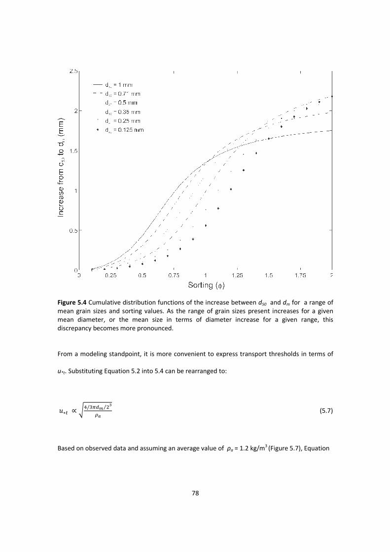
Figure 5.4 Cumulative distribution functions of the increase between mean grain sizes and sorting values. As themean diameter, or the mean size in terms of diameter increase for a given range, this discrepancy becomes more pronounced.

From a modeling standpoint, it is more convenient to express transport threshold

u*t. Substituting Equation 5.2 into 5.4

�∗� ∝ �2/��45 '⁄ 6�

Based on observed data and assuming an average value of

78

Cumulative distribution functions of the increase between d50 and mean grain sizes and sorting values. As the range of grain sizes present increases for a given mean diameter, or the mean size in terms of diameter increase for a given range, this discrepancy becomes more pronounced.

From a modeling standpoint, it is more convenient to express transport threshold

Substituting Equation 5.2 into 5.4 can be rearranged to:

Based on observed data and assuming an average value of ρa = 1.2 kg/m3 (Figure 5.7), Equation

and dm for a range of range of grain sizes present increases for a given

mean diameter, or the mean size in terms of diameter increase for a given range, this

From a modeling standpoint, it is more convenient to express transport thresholds in terms of

(5.7)

(Figure 5.7), Equation

Figure 5.5 Shear stress versus d

5.7 can be approximated by:

�∗� ) 0.97 ∗ �2 �⁄ �45 '⁄ 6� - 0

5.4 Conclusions

The goal of this study was to develop a model of aeolian transport thresholds for quartz

sand grains that predicts threshold shear velocity bas

influence of grain size-range. This was accomplished by defining grain size in terms of the

79

Shear stress versus d50 and dm, and errors associated with a linear fit.

be approximated by:

0.2

The goal of this study was to develop a model of aeolian transport thresholds for quartz

sand grains that predicts threshold shear velocity based on grain mass and encapsulates the

range. This was accomplished by defining grain size in terms of the

, and errors associated with a linear fit.

(5.8)

The goal of this study was to develop a model of aeolian transport thresholds for quartz

ed on grain mass and encapsulates the

range. This was accomplished by defining grain size in terms of the

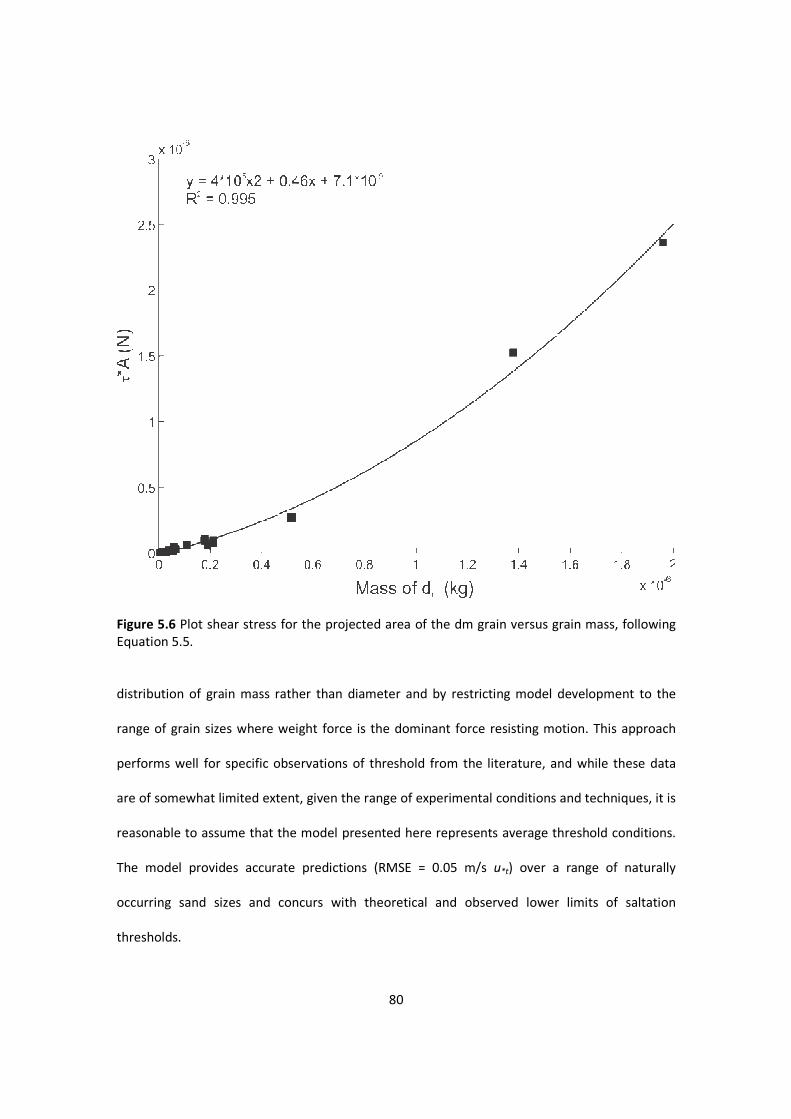
Figure 5.6 Plot shear stress for the projected area of the dm grain versus grain mass, following Equation 5.5. distribution of grain mass rather than diameter and by restricting model development to the

range of grain sizes where weight force is the dominant force resisting motion. This approach

performs well for specific observations of threshold from the literature, and whi

are of somewhat limited extent, given the range of experimental conditions and techniques, it is

reasonable to assume that the model presented here represents average threshold conditions.

The model provides accurate predictions (RMSE = 0.05

occurring sand sizes and concurs with theoretical and observed lower limits of saltation

thresholds.

80

Plot shear stress for the projected area of the dm grain versus grain mass, following

n of grain mass rather than diameter and by restricting model development to the

range of grain sizes where weight force is the dominant force resisting motion. This approach

performs well for specific observations of threshold from the literature, and whi

are of somewhat limited extent, given the range of experimental conditions and techniques, it is

reasonable to assume that the model presented here represents average threshold conditions.

The model provides accurate predictions (RMSE = 0.05 m/s u*t) over a range of naturally

occurring sand sizes and concurs with theoretical and observed lower limits of saltation

Plot shear stress for the projected area of the dm grain versus grain mass, following

n of grain mass rather than diameter and by restricting model development to the

range of grain sizes where weight force is the dominant force resisting motion. This approach

performs well for specific observations of threshold from the literature, and while these data

are of somewhat limited extent, given the range of experimental conditions and techniques, it is

reasonable to assume that the model presented here represents average threshold conditions.

) over a range of naturally

occurring sand sizes and concurs with theoretical and observed lower limits of saltation

Figure 5.7 Plot of Equation 5.7 and 5.8 for observed data for where dm is measured in mmtheoretical and observed saltation threshold (0.2 m/s) in terms of threshold shear velocity (Merrsion, 2011), and there is a near one to one relationship between the square root of the ratio of grain volume to density of air and threshold shear velocity.

5.5 References

Bagnold RA. 1936. The movement of desert sand. Proceedings of tA157, 594-620. Bagnold RA. 1941. The physics of blown Belly P-Y. 1964. Sand Movement by Wind. Technical Memorandum 1, U.S. Army Corps of Eng CERC, 38p. Chepil, WS. 1945. Dynamic of wind erosion: II, Initiation of soil movement. Soil Science 60, 397411.

81

Plot of Equation 5.7 and 5.8 for observed data for r in units of a) m and b) mmis measured in mm. Here, the coefficient 0.2 m/s is equivalent to the lower limit of

theoretical and observed saltation threshold (0.2 m/s) in terms of threshold shear velocity (Merrsion, 2011), and there is a near one to one relationship between the square root of the

io of grain volume to density of air and threshold shear velocity.

1936. The movement of desert sand. Proceedings of the Royal Society of London

he physics of blown sand and desert dunes. London, Methuen, 265 pp.

Y. 1964. Sand Movement by Wind. Technical Memorandum 1, U.S. Army Corps of Eng

Dynamic of wind erosion: II, Initiation of soil movement. Soil Science 60, 397

in units of a) m and b) mm . Here, the coefficient 0.2 m/s is equivalent to the lower limit of

theoretical and observed saltation threshold (0.2 m/s) in terms of threshold shear velocity (Merrsion, 2011), and there is a near one to one relationship between the square root of the

he Royal Society of London

Methuen, 265 pp.

Y. 1964. Sand Movement by Wind. Technical Memorandum 1, U.S. Army Corps of Eng

Dynamic of wind erosion: II, Initiation of soil movement. Soil Science 60, 397-

82

Chepil, WS. 1959. Equilibrium of soil grains at threshold of movement by wind. Soil Science Society Proceedings 23, 422-428. Cornelis WM, Gabriels D, Hartmann R. 2004. A Conceptual Model to Predict the Deflation Threshold Shear Velocity as Affected by Near-Surface Soil Water, II. Calibration and Verification. Soil Science Society of America Journal 68, 1162-1168. Davidson-Arnott RGD, Yang Y, Ollerhead J, Hesp PA, and Walker IJ. 2008. The effects of surface moisture on aeolian sediment transport threshold and mass flux on a beach. Earth Surface Processes and Landforms 33, 55-74. Greeley R, Iversen JD. 1985. Wind as a geological process: On Earth, Mars, Venus, and Titan. Cambridge University Press. Greeley R, Iversen JD, Pollack JB, Udovich N, White B. 1973 Wind tunnel studies of Martian aeolian processes. Proceedings of the Royal Society of London. Series A, Mathematical and Physical Sciences, 331-360. Greeley R, White B, Leach R, Iversen JD, Pollack J. 1976. Mars: Wind friction speeds for particle movement. Geophysical Research Letters 3, 417-420. Gregory JM, Darwish MM. 1990. Threshold friction velocity prediction considering water content. ASAE Paper No. 902562. American Society of Agricultural Engineering, St Joseph. Horikawa K, Hotta S, Kubota S. 1982. Experimental study of blown sand on a wetted sand surface. Coastal Engineering in Japan 25, 177-195. Iversen JD, White B. 1982. Saltation threshold on earth, mars and venus. Sedimentology 29, 111-119. Iversen JD, Greeley R,Pollack JB. 1976. Windblown dust on earth, Mars and Venus. Journal of Atmospheric Sciences 33, 2425-2429. Kadib A. 1965. A function for sand movement by wind. No. HEL-2-12. Hydraulics Enginnering Lab. University of California, Berkeley. Logie M. 1981. Wind tunnel experiments on dune sands. Earth Surface Processes and Landforms 6, 365-374. Logie M. 1982. Influence of roughness elements and soil moisture on on the resistance of sand to wind erosion. Catena, Supplement 1, 161-174. Lyles L, Krauss RK. 1971. Threshold velocities and initial particle motion as influenced by air turbulence Transactions of the ASAE, 14563-566. McKenna Neuman CL, Nickling WG. 1989. A theoretical and wind tunnel investigation of the effect of capillary water on the entrainment of sediment by wind. Canadian Journal of Soil Science 69, 79-96.

83

Merrison JP. 2012. Sand Transport, erosion, and granular electrification. Aeolian Research 4, 1-16. Grass AJ. 1970. Initial instability of fine bed sand. Journal of the hydraulics division 96, 619-632. Shao Y, Lu H. 2000 A simple expression for wind erosion threshold friction velocity. Journal of Geophysical Research: Atmospheres 105, 22437-22443. Sherman DJ, Li B, Farrell EJ, Ellis JT, Cox WD, Maia LP, Sousa PH. 2011. Measuring aeolian saltation: a comparison of sensors. Journal of Coastal Research 59, 280-290.

84

6. FIELD MEASURMENTS OF AEOLIAN TRANSPORT THRESHOLDS

6.1 Introduction

This chapter presents results from a series of experiments designed to field validate the

model developed in Chapter 5. Field measurements of aeolian transport were recorded at two

locations, Padre Island, TX, and St. Joseph Peninsula, FL. These locations were chosen because of

the difference in native sediment; the Padre Island sand typically has a mean grain diameter of

about 0.15 mm, and the St. Joseph Peninsula sediment is typically about twice as large in terms

of mean diameter, and thus approximately 8 times as massive. Given this discrepancy and the

basis of the model in grain mass, this was deemed a suitable range to test the validity of the

model under field conditions. The Padre Island sands are near the lower limit of natural

sediment size for which saltation is the main mode of transport, as discussed in Chapter 5, and

the St. Joseph Peninsula sand is just slightly larger than the 0.25 to 0.30 mm diameter often

cited as typical of dune sand. Further, differences in sorting (0.29 for Padre Island, 0.44 on

average for St. Joseph Peninsula) between the two sites were desirable to test the model as

well, given that determination of the mass mean (dm) is based on grain size-range.

For each location, 3-D wind measurements were recorded in conjunction with saltation

events, and data are analyzed to compare to model predictions of threshold shear velocity.

Model predictions are made based on grain size distributions of sand collected at each study site

following the method outlined in Chapter 5. In total, there are about 192 minutes of data from

St. Joseph Peninsula, and about 210 minutes of data from Padre Island, with periods of both

near-continuous and intermittent transport. Results indicate that the model performs well

under field conditions, particularly for the Padre Island data, when transport was predominantly

intermittent, and thus a large number of transport ‘on-off’ events were recorded.

85

6.2 Study Sites and Methods

The Padre Island experiment (PINS) was conducted at Padre Island National Seashore,

on Padre Island, Texas, at a site about 3 km south of the northern border of the park

(approximately 27.48°N 97.28°W, Figure 6.1). Sands at the study site consisted of very-well

sorted, fine to very fine quartz sands, with a mean grain size of approximately 0.15 mm (Figure

6.2a, Table 6.1). The berm was about 50 m wide and relatively flat (1–4°), and the beach was

backed by a 1 to 2 m foredune ridge (Figure 6.1a).

St. Joseph Peninsula (SJP) is a large spit that extends northward into the Gulf of Mexico

from the Apalachicola region of Florida (Figure 6.1). Experiments were conducted on a wide

sand flat at the distal end of the spit where there was minimal vegetation or topographic

variability (approximately 29.88°N, 85.39°W, Figure 6.1b). The distal flat was backed by an

approximately 1.5 m foredune. The sand at the field site was moderately well to well sorted

medium quartz sand, with a mean grain diameter of about 0.31 mm (Figure 6.2b, Table 6.1).

Instrumentation

Wind measurements were conducted with RM Young 8100 3D ultrasonic anemometers.

By measuring the three component (u,v,w) wind vectors, these instruments provide data

necessary to evaluate near surface turbulence. Each velocity component can be separated by

Reynolds decomposition into mean and turbulent components, so that:

� = � - �8

9 = 9 - 98

: = : - :8 (6.1)

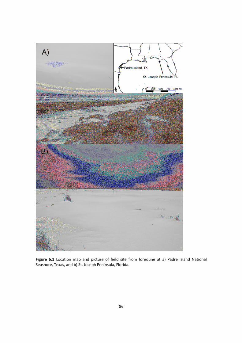
Figure 6.1 Location map and picture of field site from foredune at a) Padre Island National Seashore, Texas, and b) St. Joseph Peninsula, Florida.

86

Location map and picture of field site from foredune at a) Padre Island National Seashore, Texas, and b) St. Joseph Peninsula, Florida.

Location map and picture of field site from foredune at a) Padre Island National

87

Figure 6.2 Grain size curves of both d50 (continuous line) and dm (dashed line) shown for the a) PINS and b) SJP. dm was calculated as decribed in Chapter 5. The SJP grain size curves are average values from several sediment samples collected in the field. PINS grain characteristics were nearly identical during the field study.

where overbars denote time averaged values and primes indicate fluctuation about the mean.

Given that measurements are taken in the constant stress boundary layer, these instruments

can provide reliable measurements of Reynolds stress (RS) at the bed:

;< = =��′:′ (6.2)

and shear velocity can thus be calculated by:

�∗ = ?|�8:8| (6.3)

Before calculation of turbulent fluctuations, it is necessary to rotate the axes of the

measured wind vectors so that they are oriented with the mean flow streamline. This can be

done computationally, post-measurement (van Boxel et al. 2004) by systematically forcing the

different components to zero. The first rotation, yaw rotation, orients u into the wind direction

by requiring that 9̅, the mean transverse component, becomes zero, such that:

0

25

50

75

100

0.0 0.1 0.2 0.3 0.4

0

25

50

75

100

0 0.2 0.4 0.6 0.8

a) b)

88

�B = ��CDEF - 9�EG�F

9B = =��EG�F - 9�CDEF

:B = :�

with F = arctan MNOP (6.4)

where u0,v0, and w0 are the measured velocity data and overbars indicate time-averaged values.

The second rotation, pitch rotation, orients u along the slope of the streamline and w

perpendicular to the streamline by requiring :P to be zero, such that:

�' = �BCDE∅ - :BEG�∅

9' = 9B

:' = =�BEG�∅ - :BCDE∅

with ∅ = arctan RSNNNNOSNNNN (6.5)

The third rotation, roll rotation, is intended to orient v along the stream surfaces and w

perpendicular to the stream surfaces by requiring the covariance between them to equal zero,

such that:

�� = �'

9� = 9'CDET + :'EG�T

:� = −9'EG�T + :'CDET

with T = 0.5arctan 'M�R�NNNNNNNM��NNNNNR��NNNNNN (6.6)

89

This rotation essentially encapsulates cross-stream contributions to total stress, although they

are usually negligible in comparison with alongstream components.

Saltation events were measured with a Wenglor model YH08RCT8 fork sensor, which are

designed for counting small objects in production settings, but have been used successfully to

detect saltating grains (e.g. Davidson-Arnott et al., 2009; Sherman et al., 2011). The sensor emits

a visible (red) laser beam from one fork, and counts switch closures when detection of the beam

at the other fork is interrupted. For these experiments, the interest was simply the occurrence

of saltation, so no calibration was performed on the fork sensors in terms of total mass flux or

saltation intensity associated with switch closure counts.

Experimental Design

Data from PINS were recorded on June 10th, 2010, from approximately 1145 to 1515 hrs,

in two approximately 110 minute intervals (PINS 1 and PINS 2). Four anemometers were

mounted in sets of 2 at 2 stations on a cross-shore transect (Figure 6.3). The sampling volume of

the anemometers in each set was 35 and 140 cm from the bed, and the fork sensor sampling

path was approximately 1 cm above the bed. Data were recorded at 32 Hz using a computer

based USB data acquisition system.

Before each measurement interval, the sand surrounding Mast 1 was wetted for

approximately 5 meters in the windward direction to isolate the measurement area from the

potential influence of grains saltating from the upwind direction. A sediment sample was

collected between the two measurement intervals and standard sieving techniques were used

to produce grain statistics for input into the model of threshold shear velocity (Figure 6.2a, Table

1).

Figure 6.3 Photograph of experimental setup for PINS data. Mast 1 was approximately 5 metlandward of Mast 2 (pictured).

Two sets of data for SJP were collected on consecutive days, February 24

2010 (SJP 1 and SJP 2). Four

crossshore transect (Figure 6.5). The anemomete

bed, and a fork sensor was placed at the bed below each station. The sampling path of the fork

sensors was about 1 cm above the bed. Sediment samples were taken from each mast before

and after each measurement int

Table 6.1 Grain size statistics and transport threshold predictions and measurements for field sites

Dataset d50 (mm)

PINS 1 0.15

PINS 2 0.15

SJP 1 Mast 1 0.29

SJP 1 Mast 2 0.32

SJP 2 Mast 1 0.34

SJP 2 Mast 2 0.29

90

Photograph of experimental setup for PINS data. Mast 1 was approximately 5 met

landward of Mast 2 (pictured).

Two sets of data for SJP were collected on consecutive days, February 24

2010 (SJP 1 and SJP 2). Four anemometers were deployed in sets of 2 at 2 stations on a

crossshore transect (Figure 6.5). The anemometers were mounted at 35 and 140 cm above the

bed, and a fork sensor was placed at the bed below each station. The sampling path of the fork

sensors was about 1 cm above the bed. Sediment samples were taken from each mast before

and after each measurement interval (Figure 6.2b, Table 6.1).

Grain size statistics and transport threshold predictions and measurements for field

Measured u

Sorting (φ) dm (mm) Predicted u*t (m/s) 35 cm

0.29 0.17 0.24 0.24

0.29 0.17 0.24 0.24

0.43 0.37 0.34 0.31

0.49 0.43 0.38 0.32

0.41 0.40 0.36 0.30

0.41 0.37 0.34 0.31

Photograph of experimental setup for PINS data. Mast 1 was approximately 5 meters

Two sets of data for SJP were collected on consecutive days, February 24th and 25th,

anemometers were deployed in sets of 2 at 2 stations on a

rs were mounted at 35 and 140 cm above the

bed, and a fork sensor was placed at the bed below each station. The sampling path of the fork

sensors was about 1 cm above the bed. Sediment samples were taken from each mast before

Grain size statistics and transport threshold predictions and measurements for field

Measured u*t (m/s)

35 cm 140 cm

0.24 0.25

0.24 0.25

0.31 0.33

0.32 0.32

0.30 0.33

0.31 0.35

91

Data were logged on a stand-alone data logger at approximately 8.6 Hz, which was the

fastest scan rate allowable. This resulted in an uneven time step with respect to saltation

measurements, which were logged at 1 Hz. Subsequently, estimates of shear velocity were

resampled to 5 Hz, and then synchronized to the fork sensor measurements.

Figure 6.4 Experimental setup for SJP.

6.3 Results and Analysis

PINS Data and Analysis

During the PINS experiment, saltation occurred only at Mast 1, the landward station,

which was approximately 5 meters seaward of the foredune toe. Thus, only data from that

station are included here. For these data, the sampling volumes of Sonic 1 and Sonic 2 were

approximately 35 and 140 cm from the bed, respectively.

Figures 6.5 and 6.6 show the raw, uncorrected velocities measured by each

anemometer and the post-rotation, corrected velocities for the two PINS data collections, PINS

1 and PINS 2, respectively. The effect of the data rotations on the resultant mean flow vectors

are readily apparent. Angles of rotation from Equations 6.4-6.6 were determined from 1

Figure 6.5 Velocities of u, v, and (a-f) and after (g-l) data rotation for PINS 1 data.

minute block averages of successive velocity values. Because there were no large shifts in wind

direction during the measurement periods, this approach was satisfactory for forcing required

components to 0. Following dat

fluctuate about 0. Thus, fluctuations in

turbulent stress (RS) and shear velocity (

values of u* can be calculated by decomposing the series following Equation 6.1.

Instantaneous values of

increased slightly throughout PINS 1 and then declined slightly throughout PNS 2. In terms of

thresholds and mass flux estimates, values of

data series, would be expected to essentially maintain continuous transport at this location.

However, transport during both collection intervals was highly intermi

transport did not occur.

92

, and w (left to right) from Sonic 1 (a-c, g-i) and Sonic 2 (dl) data rotation for PINS 1 data.

minute block averages of successive velocity values. Because there were no large shifts in wind

direction during the measurement periods, this approach was satisfactory for forcing required

components to 0. Following data rotation, alongstream flow is described by

fluctuate about 0. Thus, fluctuations in u and w with respect to mean can be used to describe

) and shear velocity (u*) following Equations 6.2 and 6.3. Instantaneous

can be calculated by decomposing the series following Equation 6.1.

Instantaneous values of u* varied from near zero to about 1.5 m/s (Figure 6.7). Mean

increased slightly throughout PINS 1 and then declined slightly throughout PNS 2. In terms of

thresholds and mass flux estimates, values of u* near 1 m/s, which were common during both

data series, would be expected to essentially maintain continuous transport at this location.

However, transport during both collection intervals was highly intermittent, and fully sustained

i) and Sonic 2 (d-f, j-l) before

minute block averages of successive velocity values. Because there were no large shifts in wind

direction during the measurement periods, this approach was satisfactory for forcing required

a rotation, alongstream flow is described by u, while v and w

with respect to mean can be used to describe

) following Equations 6.2 and 6.3. Instantaneous

can be calculated by decomposing the series following Equation 6.1.

varied from near zero to about 1.5 m/s (Figure 6.7). Mean u*

increased slightly throughout PINS 1 and then declined slightly throughout PNS 2. In terms of

near 1 m/s, which were common during both

data series, would be expected to essentially maintain continuous transport at this location.

ttent, and fully sustained

Figure 6.6 Velocities of u, v, and (a-f) and after (g-l) data rotation for PINS 2 data.

On closer examination, most of the highe

high frequencies. The influence of high frequency (over 1 Hz) turbulence on aeolian transport

processes is questionable (Butterfield, 1999), so while transport thresholds may be very

frequently surpassed, if the causal oscillation is not of sufficient length in time, the influence

may be minimal. This is not surprising, given that while instantaneous stress resulting from

these high frequency fluctuations is relatively high (or low), their overall contributio

spectral power is low. Indeed, while transport events seem to be near normally distributed over

the range of u* for both PINS 1 and PINS 2 (Figures 6.8 and 6.9), there is no clear correlation

between the two, i.e. there are relatively few tra

93

, and w (left to right) from Sonic 1 (a-c, g-i) and Sonic 2 (dl) data rotation for PINS 2 data.

On closer examination, most of the highest (and lowest) values of u

high frequencies. The influence of high frequency (over 1 Hz) turbulence on aeolian transport

processes is questionable (Butterfield, 1999), so while transport thresholds may be very

the causal oscillation is not of sufficient length in time, the influence

may be minimal. This is not surprising, given that while instantaneous stress resulting from

these high frequency fluctuations is relatively high (or low), their overall contributio

spectral power is low. Indeed, while transport events seem to be near normally distributed over

for both PINS 1 and PINS 2 (Figures 6.8 and 6.9), there is no clear correlation

between the two, i.e. there are relatively few transport events associated with high levels of

i) and Sonic 2 (d-f, j-l) before

u* occur at relatively

high frequencies. The influence of high frequency (over 1 Hz) turbulence on aeolian transport

processes is questionable (Butterfield, 1999), so while transport thresholds may be very

the causal oscillation is not of sufficient length in time, the influence

may be minimal. This is not surprising, given that while instantaneous stress resulting from

these high frequency fluctuations is relatively high (or low), their overall contribution in terms of

spectral power is low. Indeed, while transport events seem to be near normally distributed over

for both PINS 1 and PINS 2 (Figures 6.8 and 6.9), there is no clear correlation

nsport events associated with high levels of u*.

Figure 6.7 Instantaneous threshold shear velocity for a) Sonic 1, b) Sonic 2, and c) transport measurements from PINS 1 data.

This strongly suggests that transport events result from relatively low frequ

velocity and u*.

Based on spectral analysis, it was determined that for PINS 1 and 2, transport occurred

predominantly at frequencies of approximately 0.19 and 0.023 Hz, or on time intervals of about

5 and 44 seconds. Similarly, power

spectra. Based on these observations, instantaneous values of

frequency components that did not appear to correlate to transport (FIR lowpass filter, Kaiser

window, 0.2 Hz cutoff) (Figure 6.10). R

of identifying transport thresholds, and in terms of validating the model developed in Chapter 5.

First, there is a clearly defined lower boundary of saltation thresho

94

Instantaneous threshold shear velocity for a) Sonic 1, b) Sonic 2, and c) transport measurements from PINS 1 data.

This strongly suggests that transport events result from relatively low frequency changes in wind

Based on spectral analysis, it was determined that for PINS 1 and 2, transport occurred

predominantly at frequencies of approximately 0.19 and 0.023 Hz, or on time intervals of about

5 and 44 seconds. Similarly, power was highly concentrated in the lowest frequencies of

spectra. Based on these observations, instantaneous values of u* were filtered to remove higher

frequency components that did not appear to correlate to transport (FIR lowpass filter, Kaiser

Hz cutoff) (Figure 6.10). Results of this transformation are very promising in terms

of identifying transport thresholds, and in terms of validating the model developed in Chapter 5.

First, there is a clearly defined lower boundary of saltation thresholds (Figures 6.11

Instantaneous threshold shear velocity for a) Sonic 1, b) Sonic 2, and c) transport

ency changes in wind

Based on spectral analysis, it was determined that for PINS 1 and 2, transport occurred

predominantly at frequencies of approximately 0.19 and 0.023 Hz, or on time intervals of about

was highly concentrated in the lowest frequencies of u*

were filtered to remove higher

frequency components that did not appear to correlate to transport (FIR lowpass filter, Kaiser

esults of this transformation are very promising in terms

of identifying transport thresholds, and in terms of validating the model developed in Chapter 5.

lds (Figures 6.11

Figure 6.8 Transport versus shear velocity for a) Sonic 1 and b) Sonic 2 from PINS 1 data.

Figure 6.9 Transport versus shear velocity for a) Sonic 1 and b) Sonic 2 from PINS 2 data.

and 6.12). Above this limit, transport events appea

The existence of these two separate axes of correlation indicates that physically, once threshold

is surpassed, transport occurs over the range of higher values of

cease causing transport. Basically, transport continues to occur after threshold conditions have

been reached if u* continues to increase. Second, the value of the threshold boundary, taken as

the average of the minimum value of

95

Transport versus shear velocity for a) Sonic 1 and b) Sonic 2 from PINS 1 data.

Transport versus shear velocity for a) Sonic 1 and b) Sonic 2 from PINS 2 data.

and 6.12). Above this limit, transport events appear near normal over the remaining range of

The existence of these two separate axes of correlation indicates that physically, once threshold

is surpassed, transport occurs over the range of higher values of u* until u

g transport. Basically, transport continues to occur after threshold conditions have

continues to increase. Second, the value of the threshold boundary, taken as

the average of the minimum value of u* for each discrete number of counts f

Transport versus shear velocity for a) Sonic 1 and b) Sonic 2 from PINS 1 data.

Transport versus shear velocity for a) Sonic 1 and b) Sonic 2 from PINS 2 data.

r near normal over the remaining range of u*.

The existence of these two separate axes of correlation indicates that physically, once threshold

u* falls sufficiently to

g transport. Basically, transport continues to occur after threshold conditions have

continues to increase. Second, the value of the threshold boundary, taken as

for each discrete number of counts from the fork

Figure 6.10 Filtered shear velocity for a) Sonic 1 and b) Sonic 2 for PINS 1 data.

sensor, agrees very well with predictions from the model based on the grain size

PINS sand. (Table 6.1).

SJP Data and Analysis

For the SJP experiment, transport was near continuous for much of SJP 1 and

intermittent for SJP 2 (Figure 6.13 and 6.14). Similarly to the PINS data, transport occurred at

relatively low frequencies of about 0.36 and 0.012 Hz, or about 3 and 80 seconds in time, and

transport events are widely distributed across the range of instantaneous

6.16). Shear velocity data were filtered according to transport and

0.05 Hz cutoff ) Figure 6.17).

The filtered u* are better correlat

there is not a sharp threshold boundary as was evident in the PINS data (Figure 6.18 and 6.19).

There do appear to be lower thresholds bounds at about 0.25 m/s for SJP 1 and 0.22 to 0.28 m/s

for SJP 2, but they are not distinct as was the case with the PINS data. Instead, transport events

96

Filtered shear velocity for a) Sonic 1 and b) Sonic 2 for PINS 1 data.

sensor, agrees very well with predictions from the model based on the grain size

periment, transport was near continuous for much of SJP 1 and

intermittent for SJP 2 (Figure 6.13 and 6.14). Similarly to the PINS data, transport occurred at

relatively low frequencies of about 0.36 and 0.012 Hz, or about 3 and 80 seconds in time, and

nsport events are widely distributed across the range of instantaneous

6.16). Shear velocity data were filtered according to transport and u* (FIR filter, Kaiser window,

0.05 Hz cutoff ) Figure 6.17).

are better correlated with transport than instantaneous values were, but

there is not a sharp threshold boundary as was evident in the PINS data (Figure 6.18 and 6.19).

There do appear to be lower thresholds bounds at about 0.25 m/s for SJP 1 and 0.22 to 0.28 m/s

but they are not distinct as was the case with the PINS data. Instead, transport events

Filtered shear velocity for a) Sonic 1 and b) Sonic 2 for PINS 1 data.

sensor, agrees very well with predictions from the model based on the grain size-range of the

periment, transport was near continuous for much of SJP 1 and

intermittent for SJP 2 (Figure 6.13 and 6.14). Similarly to the PINS data, transport occurred at

relatively low frequencies of about 0.36 and 0.012 Hz, or about 3 and 80 seconds in time, and

nsport events are widely distributed across the range of instantaneous u* (Figure 6.15 and

(FIR filter, Kaiser window,

ed with transport than instantaneous values were, but

there is not a sharp threshold boundary as was evident in the PINS data (Figure 6.18 and 6.19).

There do appear to be lower thresholds bounds at about 0.25 m/s for SJP 1 and 0.22 to 0.28 m/s

but they are not distinct as was the case with the PINS data. Instead, transport events

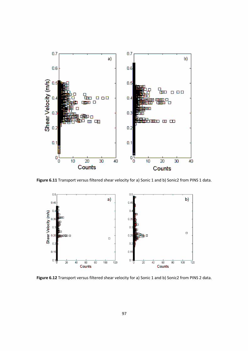
Figure 6.11 Transport versus filtered shear velocity for a) Sonic 1 and b) Sonic2 from PINS 1 data.

Figure 6.12 Transport versus filtered shear velocity for a) Son

97

Transport versus filtered shear velocity for a) Sonic 1 and b) Sonic2 from PINS 1 data.

Transport versus filtered shear velocity for a) Sonic 1 and b) Sonic2 from PINS 2 data.

Transport versus filtered shear velocity for a) Sonic 1 and b) Sonic2 from PINS 1 data.

ic 1 and b) Sonic2 from PINS 2 data.

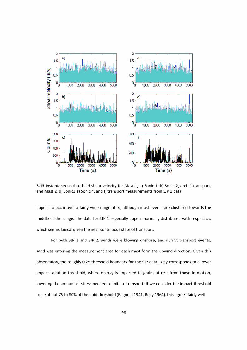
6.13 Instantaneous threshold shear velocity for Mast 1, a) Sonic 1, b) Sonic 2, and c) transport, and Mast 2, d) Sonic3 e) Sonic 4, and f) transport measurements from SJP 1 data.

appear to occur over a fairly wide

middle of the range. The data for SJP 1 especially appear normally distributed with respect

which seems logical given the near continuous state of transport.

For both SJP 1 and SJP 2, winds w

sand was entering the measurement area for each mast form the upwind direction. Given this

observation, the roughly 0.25 threshold boundary for the SJP data likely corresponds to a lower

impact saltation threshold, where energy is imparted to grains at res

lowering the amount of stress needed to initiate transport. If we consider the impact threshold

to be about 75 to 80% of the fluid threshold (Bagnold 1941, Belly 1964), this agrees

98

Instantaneous threshold shear velocity for Mast 1, a) Sonic 1, b) Sonic 2, and c) transport, and Mast 2, d) Sonic3 e) Sonic 4, and f) transport measurements from SJP 1 data.

appear to occur over a fairly wide range of u*, although most events are clustered towards the

middle of the range. The data for SJP 1 especially appear normally distributed with respect

which seems logical given the near continuous state of transport.

For both SJP 1 and SJP 2, winds were blowing onshore, and during transport events,

sand was entering the measurement area for each mast form the upwind direction. Given this

observation, the roughly 0.25 threshold boundary for the SJP data likely corresponds to a lower

hreshold, where energy is imparted to grains at rest from those in motion,

lowering the amount of stress needed to initiate transport. If we consider the impact threshold

to be about 75 to 80% of the fluid threshold (Bagnold 1941, Belly 1964), this agrees

Instantaneous threshold shear velocity for Mast 1, a) Sonic 1, b) Sonic 2, and c) transport, and Mast 2, d) Sonic3 e) Sonic 4, and f) transport measurements from SJP 1 data.

, although most events are clustered towards the

middle of the range. The data for SJP 1 especially appear normally distributed with respect u*,

ere blowing onshore, and during transport events,

sand was entering the measurement area for each mast form the upwind direction. Given this

observation, the roughly 0.25 threshold boundary for the SJP data likely corresponds to a lower

from those in motion,

lowering the amount of stress needed to initiate transport. If we consider the impact threshold

to be about 75 to 80% of the fluid threshold (Bagnold 1941, Belly 1964), this agrees fairly well

6.14 Instantaneous threshold shear velocity for Mast 1, a) Sonic 1, b) Sonic 2, and c) transport, and Mast 2, d) Sonic3 e) Sonic 4, and f) transport measurements from SJP 2 data.

with the predicted fluid threshold for each mast and data set

value of u* for all transport detections, this value also agrees well with, but in most cases

slightly lower than the predicted threshold for each mast and data set. Overall the evidence

indicates that the system was mixe

that the average value of shear velocity for each transport detection is a fair indicator of

threshold conditions for these data.

99

Instantaneous threshold shear velocity for Mast 1, a) Sonic 1, b) Sonic 2, and c) transport, and Mast 2, d) Sonic3 e) Sonic 4, and f) transport measurements from SJP 2 data.

with the predicted fluid threshold for each mast and data set (Table 6.1). If we take the mean

for all transport detections, this value also agrees well with, but in most cases

slightly lower than the predicted threshold for each mast and data set. Overall the evidence

indicates that the system was mixed through time in terms of fluid and impact thresholds, and

that the average value of shear velocity for each transport detection is a fair indicator of

threshold conditions for these data.

Instantaneous threshold shear velocity for Mast 1, a) Sonic 1, b) Sonic 2, and c) transport, and Mast 2, d) Sonic3 e) Sonic 4, and f) transport measurements from SJP 2 data.

1). If we take the mean

for all transport detections, this value also agrees well with, but in most cases

slightly lower than the predicted threshold for each mast and data set. Overall the evidence

d through time in terms of fluid and impact thresholds, and

that the average value of shear velocity for each transport detection is a fair indicator of

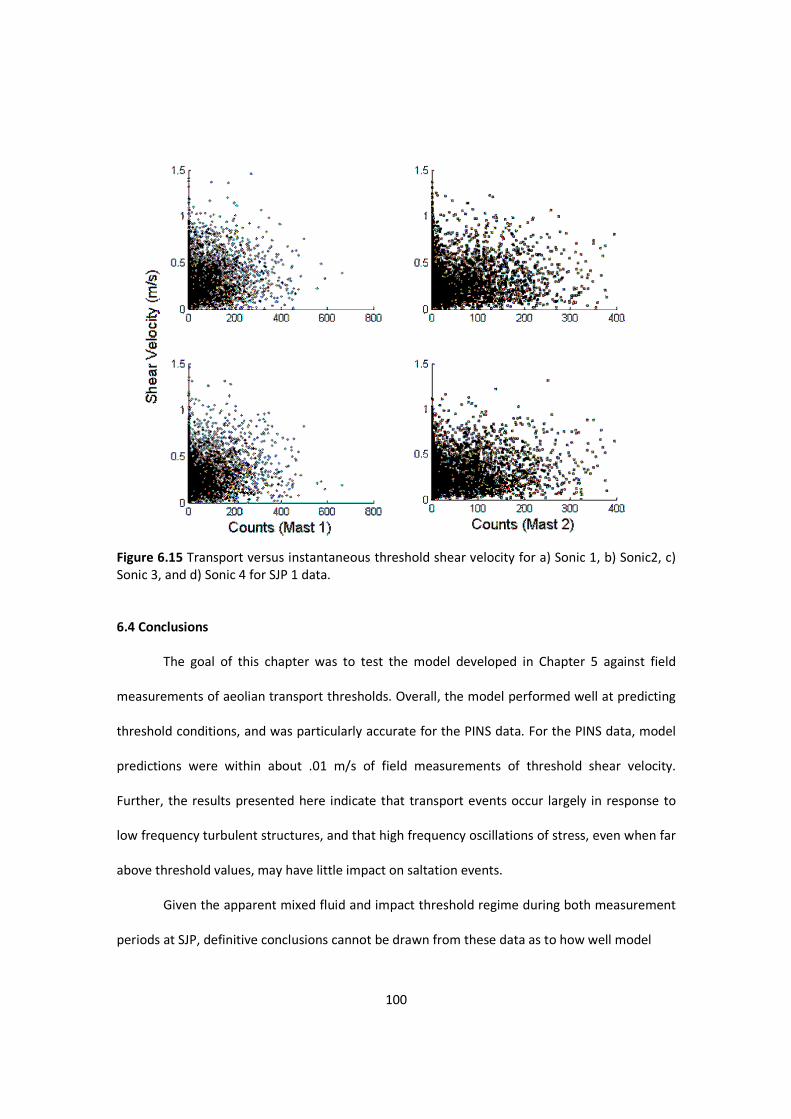
Figure 6.15 Transport versus instantaneous threshold shear vSonic 3, and d) Sonic 4 for SJP 1 data.

6.4 Conclusions

The goal of this chapter was to test the model developed in Chapter 5 against field

measurements of aeolian transport thresholds. Overall, the model performed we

threshold conditions, and was particularly accurate for the PINS data. For the PINS data, model

predictions were within about .01 m/s of field measurements of threshold shear velocity.

Further, the results presented here indicate that tran

low frequency turbulent structures, and that high frequency oscillations of stress, even when far

above threshold values, may have little impact on saltation events.

Given the apparent mixed fluid and impact thres

periods at SJP, definitive conclusions cannot be drawn from these data as to how well model

100

Transport versus instantaneous threshold shear velocity for a) Sonic 1, b) Sonic2, c) Sonic 3, and d) Sonic 4 for SJP 1 data.

The goal of this chapter was to test the model developed in Chapter 5 against field

measurements of aeolian transport thresholds. Overall, the model performed we

threshold conditions, and was particularly accurate for the PINS data. For the PINS data, model

predictions were within about .01 m/s of field measurements of threshold shear velocity.

Further, the results presented here indicate that transport events occur largely in response to

low frequency turbulent structures, and that high frequency oscillations of stress, even when far

above threshold values, may have little impact on saltation events.

Given the apparent mixed fluid and impact threshold regime during both measurement

periods at SJP, definitive conclusions cannot be drawn from these data as to how well model

elocity for a) Sonic 1, b) Sonic2, c)

The goal of this chapter was to test the model developed in Chapter 5 against field

measurements of aeolian transport thresholds. Overall, the model performed well at predicting

threshold conditions, and was particularly accurate for the PINS data. For the PINS data, model

predictions were within about .01 m/s of field measurements of threshold shear velocity.

sport events occur largely in response to

low frequency turbulent structures, and that high frequency oscillations of stress, even when far

hold regime during both measurement

periods at SJP, definitive conclusions cannot be drawn from these data as to how well model

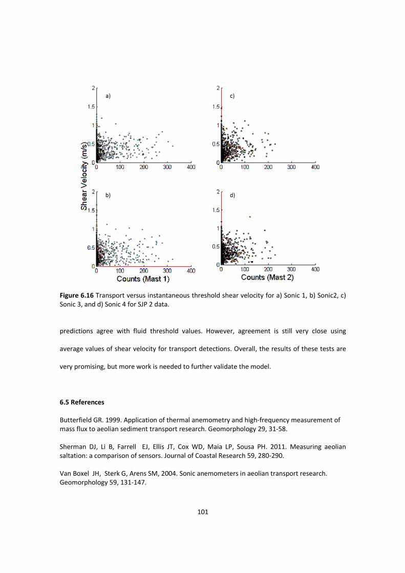
Figure 6.16 Transport versus instantaneous threshold shear velocity for a) Sonic 1, b) Sonic2, c) Sonic 3, and d) Sonic 4 for SJP 2 data.

predictions agree with fluid threshold values. However, agreement is still very close using

average values of shear velocity for transport detections. Overall, the results of these tests are

very promising, but more work is needed to further

6.5 References

Butterfield GR. 1999. Application of thermal anemometry and highmass flux to aeolian sediment transp Sherman DJ, Li B, Farrell EJ, Ellis JT, Cox WDsaltation: a comparison of sensors. Journal of Coastal Research Van Boxel JH, Sterk G, ArensGeomorphology 59, 131-147.

101

Transport versus instantaneous threshold shear velocity for a) Sonic 1, b) Sonic2, c) SJP 2 data.

predictions agree with fluid threshold values. However, agreement is still very close using

average values of shear velocity for transport detections. Overall, the results of these tests are

very promising, but more work is needed to further validate the model.

Butterfield GR. 1999. Application of thermal anemometry and high-frequency measurement of mass flux to aeolian sediment transport research. Geomorphology 29, 31-58.

, Farrell EJ, Ellis JT, Cox WD, Maia LP, Sousa PH. 2011. Measuring aeolian saltation: a comparison of sensors. Journal of Coastal Research 59, 280-290.

Arens SM, 2004. Sonic anemometers in aeolian trans147.

Transport versus instantaneous threshold shear velocity for a) Sonic 1, b) Sonic2, c)

predictions agree with fluid threshold values. However, agreement is still very close using

average values of shear velocity for transport detections. Overall, the results of these tests are

frequency measurement of 58.

LP, Sousa PH. 2011. Measuring aeolian

, 2004. Sonic anemometers in aeolian transport research.

102

Walker IJ. 2005. Physical and logistical considerations of using ultrasonic anemometers in aeolian sediment transport research. Geomorphology 68, 57-76.

Figure 6.17 Filtered shear velocity for a) Sonic 1, b) Sonic 2, c) Sonic 3, and d) Sonic 4 for SJP 1 data.

Figure 6.17 Filtered shear velocity for a) Sonic 1, b) Sonic 2, c) Sonic 3, and d) Sonic 4 for SJP 1 data.

103

Filtered shear velocity for a) Sonic 1, b) Sonic 2, c) Sonic 3, and d) Sonic 4 for SJP 1

Filtered shear velocity for a) Sonic 1, b) Sonic 2, c) Sonic 3, and d) Sonic 4 for SJP 1

Filtered shear velocity for a) Sonic 1, b) Sonic 2, c) Sonic 3, and d) Sonic 4 for SJP 1

Filtered shear velocity for a) Sonic 1, b) Sonic 2, c) Sonic 3, and d) Sonic 4 for SJP 1

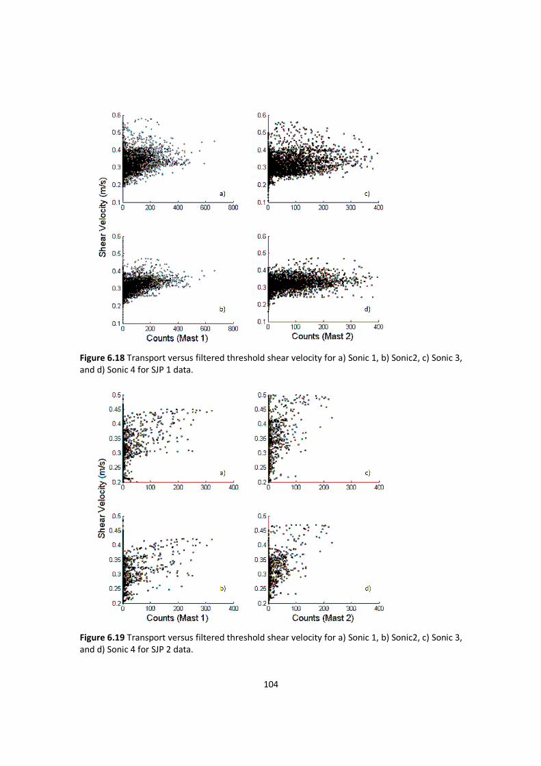
Figure 6.18 Transport versus filtered threshold shear velocity for a) Sonic 1, b) Sonic2, c) Sonic 3, and d) Sonic 4 for SJP 1 data.

Figure 6.19 Transport versus filtered threshold shear velocity for a) Sonic 1, b) Sonic2, c) Sonic 3, and d) Sonic 4 for SJP 2 data.

104

Transport versus filtered threshold shear velocity for a) Sonic 1, b) Sonic2, c) Sonic 3, and d) Sonic 4 for SJP 1 data.

Transport versus filtered threshold shear velocity for a) Sonic 1, b) Sonic2, c) Sonic 3, and d) Sonic 4 for SJP 2 data.

Transport versus filtered threshold shear velocity for a) Sonic 1, b) Sonic2, c) Sonic 3,

Transport versus filtered threshold shear velocity for a) Sonic 1, b) Sonic2, c) Sonic 3,

105

7. SUMMARY AND CONCLUSIONS

The goal of this dissertation was to advance understanding of the initiation of motion in

aeolian transport. Individual chapters focused on two key areas of concern: quantifying

spatiotemporal variability in surficial moisture, which is a limiting factor for transport processes,

and improving predictive capability for transport thresholds of dry sands. These two foci were

chosen because they represent critical components of aeolian processes where uncertainty

limits understanding of process level dynamics and ability to model aeolian systems.

The first three chapters focused on surficial moisture. There were two general

objectives for this set of studies. First, the studies were designed to examine small scale

variability in surface moisture in terms of both horizontal and vertical distributions of moisture

on a fine grained beach. Second, Chapters 3 and 4 were designed to develop improved moisture

measurement techniques for application to aeolian process studies. Most importantly, these

studies explored non-destructive methods to accurately estimate moisture in just the top few

layers of grains. Chapters 5 and 6 presented the development and field testing of a new model

for threshold conditions at the initiation of motion for quartz sands. The model was developed

based on the assumption that for sand sized grains, transport thresholds should be directly

proportional to grain weight. Further, the model also assumed that by redefining grain size

distributions in terms of mass rather than diameter, predictive accuracy would be improved.

The model was tested under field conditions at two different sites with characteristically

different grain size-ranges spanning a range representative of sand found on most

beachesbeaches, particularly in the Gulf Coast region.

Results indicate that surficial moisture in beach sands is highly variable over space and

with depth. In Chapter 2, it was found that surface moisture content can be highly variable over

small areas, with differences of up to about 14% by weight occurring within a 0.5 m2 area, which

106

indicate that there is a potential for error even over very small scales, particularly for mid ranges

of possible moisture contents. This has potentially significant ramification in terms of modeling

aeolian transport thresholds, especially considering that critical limiting values of moisture are

poorly understood. In this particular study, however, it was found that this variability would

have negligible effects on beach-wide estimates of area available to transport given theoretical

critical moisture values.

Results from Chapter 3 indicate that there is considerable variability in near surface

moisture gradients, again particularly for mid range levels of moisture typically found over most

of a natural beach. This finding reinforces the need in aeolian process studies to restrict

measurements of moisture to a very thin layer just at the surface. Further, results from Chapter

3 indicate that measurements of moisture integrated over even very shallow depths may

significantly overestimate the limiting effects of moisture on transport processes.

The handheld netradiometer developed for work presented in Chapter 5 proved to be

an accurate, simple, and reliable tool to estimate moisture at the surface of the bed. This

approach has several advantages, including simplicity, low cost, and portability. Perhaps the

most novel application would be the ability to use remote sensing technology to measure

surface moisture at night, which is not possible with other remote sensing based approaches.

The model developed in Chapter 5 appears to provide a simple, accurate method to

estimate levels of shear stress needed to initiate motion for quartz sands. The model is based on

experimental observations spanning nearly 80 years, and given the range of experimental

designs and sand sizes used to produce those data, it can be reasonably concluded that the

model provides a good estimate of average threshold conditions in terms of environmental

conditions (.e.g. humidity, air density, temperature) over the range of sand sized grains

commonly found in natural environments. Results from the field tests presented in Chapter 6

107

indicate that the model performs well for natural sands, but more work is needed to test this

model under a larger variety of sand sizes and environmental conditions.

Overall, the work presented in this dissertation provides significant advances in the

study aoelian transport systems. These studies have provided critical analysis of current trends

in beach surface moisture monitoring, improved our understanding of spatiotemporal variability

in surficial moisture on beaches, and discussed improved technologies for measuring moisture

at the surface of the sediment bed. Further, the model of transport thresholds presented

represents a potential shift in the way aeolian systems are modeled as a whole, and should

provide increased accuracy for threshold and mass flux models.

108

APPENDIX 1: PERMISSION TO REPRODUCE CHAPTER 3 FOR THIS DISSERTATION

Dear Brandon: Please accept this letter as permission to reproduce the JCR paper in reformatted form in your dissertation. There is no fee for this permission. All we ask is for a proper citation as to the original source of publication. Good luck with the your project. Sincerely, Charlie Finkl Charles W. Finkl, Ph.D. President & Executive Director The Coastal Education & Research Foundation, Inc. [CERF] Editor-in-Chief Journal of Coastal Research (JCR) Professor Emeritus Department of Geosciences Florida Atlantic University 1656 Cypress Row Drive West Palm Beach, FL 33411, USA http://www.cerf-jcr.org/ CFinkl@CERF-JCR.com (561) 313-0926 Dr. Finkl, Thank you for your recent acceptance of the below article. I do have one request regarding this manuscript. I have chosen to write a journal style dissertation, and this manuscript is one of the articles slated to be included. However, LSU requires that I receive written copyright permission from the appropriate journal to use any article that has already been published, or has been accepted for publication. This is because the whole dissertation will be publicly available on the LSU libraries electronic thesis and dissertation database, which technically means it will be republished. Of course, each article will be reformatted to the LSU Graduate School dissertation specifications, but the overwhelming majority of the text and figures will remain the same. Thank you again, and I am sorry for any inconvenience. Ms. No. JCOASTRES-D-12-00008R1 Comparison of surface moisture measurements to depth-integrated moisture measurements on a fine-grained beach Journal of Coastal Research

109

APPENDIX 2: PERMISSION TO REPRODUCE CHAPTER 2 FOR THIS DISSERTATION

JOHN WILEY AND SONS LICENSE

TERMS AND CONDITIONS

Mar 19, 2012

This is a License Agreement between Brandon L Edwards ("You") and John Wiley and Sons ("John Wiley and Sons") provided by Copyright Clearance Center ("CCC"). The license consists of your order details, the terms and conditions provided by John Wiley and Sons, and the payment terms and conditions.

All payments must be made in full to CCC. For payment instructions, please see information

listed at the bottom of this form.

License Number 2872560448132

License date Mar 19, 2012

Licensed content publisher John Wiley and Sons

Licensed content publication Earth Surface Processes and Landforms

Licensed content title Small-scale variability in surface moisture on a fine-grained beach: implications for modeling aeolian transport

Licensed content author Brandon L. Edwards,Steven L. Namikas

Licensed content date Aug 1, 2009

Start page 1333

End page 1338

Type of use Dissertation/Thesis

Requestor type Author of this Wiley article

Format Print and electronic

Portion Full article

Will you be translating? No

Order reference number

Total 0.00 USD

Terms and Conditions

110

TERMS AND CONDITIONS This copyrighted material is owned by or exclusively licensed to John Wiley & Sons, Inc. or one of its group companies (each a "Wiley Company") or a society for whom a Wiley Company has exclusive publishing rights in relation to a particular journal (collectively WILEY"). By clicking "accept" in connection with completing this licensing transaction, you agree that the following terms and conditions apply to this transaction (along with the billing and payment terms and conditions established by the Copyright Clearance Center Inc., ("CCC’s Billing and Payment terms and conditions"), at the time that you opened your Rightslink account (these are available at any time at http://myaccount.copyright.com) Terms and Conditions 1. The materials you have requested permission to reproduce (the "Materials") are protected by copyright. 2. You are hereby granted a personal, non-exclusive, non-sublicensable, non-transferable, worldwide, limited license to reproduce the Materials for the purpose specified in the licensing process. This license is for a one-time use only with a maximum distribution equal to the number that you identified in the licensing process. Any form of republication granted by this licence must be completed within two years of the date of the grant of this licence (although copies prepared before may be distributed thereafter). The Materials shall not be used in any other manner or for any other purpose. Permission is granted subject to an appropriate acknowledgement given to the author, title of the material/book/journal and the publisher. You shall also duplicate the copyright notice that appears in the Wiley publication in your use of the Material. Permission is also granted on the understanding that nowhere in the text is a previously published source acknowledged for all or part of this Material. Any third party material is expressly excluded from this permission. 3. With respect to the Materials, all rights are reserved. Except as expressly granted by the terms of the license, no part of the Materials may be copied, modified, adapted (except for minor reformatting required by the new Publication), translated, reproduced, transferred or distributed, in any form or by any means, and no derivative works may be made based on the Materials without the prior permission of the respective copyright owner. You may not alter, remove or suppress in any manner any copyright, trademark or other notices displayed by the Materials. You may not license, rent, sell, loan, lease, pledge, offer as security, transfer or assign the Materials, or any of the rights granted to you hereunder to any other person. 4. The Materials and all of the intellectual property rights therein shall at all times remain the exclusive property of John Wiley & Sons Inc or one of its related companies (WILEY) or their respective licensors, and your interest therein is only that of having possession of and the right to reproduce the Materials pursuant to Section 2 herein during the continuance of this Agreement. You agree that you own no right, title or interest in or to the Materials or any of the intellectual property rights therein. You shall have no rights hereunder other than the license as provided for above in Section 2. No right, license or interest to any trademark, trade name, service mark or other branding ("Marks") of WILEY or its licensors is granted hereunder, and you agree that you shall not assert any such right, license or interest with respect thereto.

111

5. NEITHER WILEY NOR ITS LICENSORS MAKES ANY WARRANTY OR REPRESENTATION OF ANY KIND TO YOU OR ANY THIRD PARTY, EXPRESS, IMPLIED OR STATUTORY, WITH RESPECT TO THE MATERIALS OR THE ACCURACY OF ANY INFORMATION CONTAINED IN THE MATERIALS, INCLUDING, WITHOUT LIMITATION, ANY IMPLIED WARRANTY OF MERCHANTABILITY, ACCURACY, SATISFACTORY QUALITY, FITNESS FOR A PARTICULAR PURPOSE, USABILITY, INTEGRATION OR NON-INFRINGEMENT AND ALL SUCH WARRANTIES ARE HEREBY EXCLUDED BY WILEY AND ITS LICENSORS AND WAIVED BY YOU. 6. WILEY shall have the right to terminate this Agreement immediately upon breach of this Agreement by you. 7. You shall indemnify, defend and hold harmless WILEY, its Licensors and their respective directors, officers, agents and employees, from and against any actual or threatened claims, demands, causes of action or proceedings arising from any breach of this Agreement by you. 8. IN NO EVENT SHALL WILEY OR ITS LICENSORS BE LIABLE TO YOU OR ANY OTHER PARTY OR ANY OTHER PERSON OR ENTITY FOR ANY SPECIAL, CONSEQUENTIAL, INCIDENTAL, INDIRECT, EXEMPLARY OR PUNITIVE DAMAGES, HOWEVER CAUSED, ARISING OUT OF OR IN CONNECTION WITH THE DOWNLOADING, PROVISIONING, VIEWING OR USE OF THE MATERIALS REGARDLESS OF THE FORM OF ACTION, WHETHER FOR BREACH OF CONTRACT, BREACH OF WARRANTY, TORT, NEGLIGENCE, INFRINGEMENT OR OTHERWISE (INCLUDING, WITHOUT LIMITATION, DAMAGES BASED ON LOSS OF PROFITS, DATA, FILES, USE, BUSINESS OPPORTUNITY OR CLAIMS OF THIRD PARTIES), AND WHETHER OR NOT THE PARTY HAS BEEN ADVISED OF THE POSSIBILITY OF SUCH DAMAGES. THIS LIMITATION SHALL APPLY NOTWITHSTANDING ANY FAILURE OF ESSENTIAL PURPOSE OF ANY LIMITED REMEDY PROVIDED HEREIN. 9. Should any provision of this Agreement be held by a court of competent jurisdiction to be illegal, invalid, or unenforceable, that provision shall be deemed amended to achieve as nearly as possible the same economic effect as the original provision, and the legality, validity and enforceability of the remaining provisions of this Agreement shall not be affected or impaired thereby. 10. The failure of either party to enforce any term or condition of this Agreement shall not constitute a waiver of either party's right to enforce each and every term and condition of this Agreement. No breach under this agreement shall be deemed waived or excused by either party unless such waiver or consent is in writing signed by the party granting such waiver or consent. The waiver by or consent of a party to a breach of any provision of this Agreement shall not operate or be construed as a waiver of or consent to any other or subsequent breach by such other party. 11. This Agreement may not be assigned (including by operation of law or otherwise) by you without WILEY's prior written consent. 12. Any fee required for this permission shall be non-refundable after thirty (30) days from receipt. 13. These terms and conditions together with CCC’s Billing and Payment terms and conditions (which are incorporated herein) form the entire agreement between you and WILEY concerning this licensing transaction and (in the absence of fraud) supersedes all prior agreements and representations of the parties, oral or written. This Agreement may not be amended except in

112

writing signed by both parties. This Agreement shall be binding upon and inure to the benefit of the parties' successors, legal representatives, and authorized assigns. 14. In the event of any conflict between your obligations established by these terms and conditions and those established by CCC’s Billing and Payment terms and conditions, these terms and conditions shall prevail. 15. WILEY expressly reserves all rights not specifically granted in the combination of (i) the license details provided by you and accepted in the course of this licensing transaction, (ii) these terms and conditions and (iii) CCC’s Billing and Payment terms and conditions. 16. This Agreement will be void if the Type of Use, Format, Circulation, or Requestor Type was misrepresented during the licensing process. 17. This Agreement shall be governed by and construed in accordance with the laws of the State of New York, USA, without regards to such state’s conflict of law rules. Any legal action, suit or proceeding arising out of or relating to these Terms and Conditions or the breach thereof shall be instituted in a court of competent jurisdiction in New York County in the State of New York in the United States of America and each party hereby consents and submits to the personal jurisdiction of such court, waives any objection to venue in such court and consents to service of process by registered or certified mail, return receipt requested, at the last known address of such party. Wiley Open Access Terms and Conditions All research articles published in Wiley Open Access journals are fully open access: immediately freely available to read, download and share. Articles are published under the terms of the Creative Commons Attribution Non Commercial License. which permits use, distribution and reproduction in any medium, provided the original work is properly cited and is not used for commercial purposes. The license is subject to the Wiley Open Access terms and conditions: Wiley Open Access articles are protected by copyright and are posted to repositories and websites in accordance with the terms of the Creative Commons Attribution Non Commercial License. At the time of deposit, Wiley Open Access articles include all changes made during peer review, copyediting, and publishing. Repositories and websites that host the article are responsible for incorporating any publisher-supplied amendments or retractions issued subsequently. Wiley Open Access articles are also available without charge on Wiley's publishing platform, Wiley

Online Library or any successor sites. Use by non-commercial users For non-commercial and non-promotional purposes individual users may access, download, copy, display and redistribute to colleagues Wiley Open Access articles, as well as adapt, translate, text- and data-mine the content subject to the following conditions:

The authors' moral rights are not compromised. These rights include the right of "paternity" (also known as "attribution" - the right for the author to be identified as such) and "integrity" (the right for the author not to have the work altered in such a way that the author's reputation or integrity may be impugned).

113

Where content in the article is identified as belonging to a third party, it is the obligation of the user to ensure that any reuse complies with the copyright policies of the owner of that content. If article content is copied, downloaded or otherwise reused for non-commercial research and education purposes, a link to the appropriate bibliographic citation (authors, journal, article title, volume, issue, page numbers, DOI and the link to the definitive published version on Wiley Online Library) should be maintained. Copyright notices and disclaimers must not be deleted. Any translations, for which a prior translation agreement with Wiley has not been agreed, must prominently display the statement: "This is an unofficial translation of an article that appeared in a Wiley publication. The publisher has not endorsed this translation." Use by commercial "for-profit" organisations Use of Wiley Open Access articles for commercial, promotional, or marketing purposes requires further explicit permission from Wiley and will be subject to a fee. Commercial purposes include:

Copying or downloading of articles, or linking to such articles for further redistribution, sale or licensing; Copying, downloading or posting by a site or service that incorporates advertising with such content; The inclusion or incorporation of article content in other works or services (other than normal quotations with an appropriate citation) that is then available for sale or licensing, for a fee (for example, a compilation produced for marketing purposes, inclusion in a sales pack) Use of article content (other than normal quotations with appropriate citation) by for-profit organisations for promotional purposes Linking to article content in e-mails redistributed for promotional, marketing or educational purposes; Use for the purposes of monetary reward by means of sale, resale, licence, loan, transfer or other form of commercial exploitation such as marketing products Print reprints of Wiley Open Access articles can be purchased from: corporatesales@wiley.com Other Terms and Conditions: BY CLICKING ON THE "I AGREE..." BOX, YOU ACKNOWLEDGE THAT YOU HAVE READ AND FULLY UNDERSTAND EACH OF THE SECTIONS OF AND PROVISIONS SET FORTH IN THIS AGREEMENT AND THAT YOU ARE IN AGREEMENT WITH AND ARE WILLING TO ACCEPT ALL OF YOUR OBLIGATIONS AS SET FORTH IN THIS AGREEMENT. v1.7

If you would like to pay for this license now, please remit this license along with your payment

made payable to "COPYRIGHT CLEARANCE CENTER" otherwise you will be invoiced within 48

hours of the license date. Payment should be in the form of a check or money order referencing

your account number and this invoice number RLNK500742303.

Once you receive your invoice for this order, you may pay your invoice by credit card. Please

follow instructions provided at that time.

Make Payment To:

Copyright Clearance Center

114

Dept 001

P.O. Box 843006

Boston, MA 02284-3006

For suggestions or comments regarding this order, contact RightsLink Customer Support:

customercare@copyright.com or +1-877-622-5543 (toll free in the US) or +1-978-646-2777.

Gratis licenses (referencing $0 in the Total field) are free. Please retain this printable license for

your reference. No payment is required.

115

APPENDIX 3: PERMISSION TO REPRODUCE CHAPTER 4 FOR THIS DISSERTATION

JOHN WILEY AND SONS LICENSE

TERMS AND CONDITIONS

Jun 13, 2013

This is a License Agreement between Brandon L Edwards ("You") and John Wiley and Sons ("John Wiley and Sons") provided by Copyright Clearance Center ("CCC"). The license consists of your order details, the terms and conditions provided by John Wiley and Sons, and the payment terms and conditions.

All payments must be made in full to CCC. For payment instructions, please see information

listed at the bottom of this form.

License Number 3167141044132

License date Jun 13, 2013

Licensed content publisher John Wiley and Sons

Licensed content publication Earth Surface Processes and Landforms

Licensed content title Simple infrared techniques for measuring beach surface moisture

Licensed copyright line Copyright © 2012 John Wiley & Sons, Ltd.

Licensed content author Brandon L. Edwards,Steven L. Namikas,Eurico J. D&apos;Sa

Licensed content date Oct 4, 2012

Start page 192

End page 197

Type of use Dissertation/Thesis

Requestor type Author of this Wiley article

Format Electronic

Portion Full article

Will you be translating? No

Total 0.00 USD

Terms and Conditions

TERMS AND CONDITIONS

This copyrighted material is owned by or exclusively licensed to John Wiley & Sons, Inc. or one of

116

its group companies (each a "Wiley Company") or a society for whom a Wiley Company has exclusive publishing rights in relation to a particular journal (collectively "WILEY"). By clicking "accept" in connection with completing this licensing transaction, you agree that the following terms and conditions apply to this transaction (along with the billing and payment terms and conditions established by the Copyright Clearance Center Inc., ("CCC's Billing and Payment terms and conditions"), at the time that you opened your RightsLink account (these are available at any time at http://myaccount.copyright.com).

Terms and Conditions

1. The materials you have requested permission to reproduce (the "Materials") are protected by copyright.

2.You are hereby granted a personal, non-exclusive, non-sublicensable, non-transferable, worldwide, limited license to reproduce the Materials for the purpose specified in the licensing process. This license is for a one-time use only with a maximum distribution equal to the number that you identified in the licensing process. Any form of republication granted by this license must be completed within two years of the date of the grant of this license (although copies prepared before may be distributed thereafter). The Materials shall not be used in any other manner or for any other purpose. Permission is granted subject to an appropriate acknowledgement given to the author, title of the material/book/journal and the publisher. You shall also duplicate the copyright notice that appears in the Wiley publication in your use of the Material. Permission is also granted on the understanding that nowhere in the text is a previously published source acknowledged for all or part of this Material. Any third party material is expressly excluded from this permission.

3. With respect to the Materials, all rights are reserved. Except as expressly granted by the terms of the license, no part of the Materials may be copied, modified, adapted (except for minor reformatting required by the new Publication), translated, reproduced, transferred or distributed, in any form or by any means, and no derivative works may be made based on the Materials without the prior permission of the respective copyright owner. You may not alter, remove or suppress in any manner any copyright, trademark or other notices displayed by the Materials. You may not license, rent, sell, loan, lease, pledge, offer as security, transfer or assign the Materials, or any of the rights granted to you hereunder to any other person.

4. The Materials and all of the intellectual property rights therein shall at all times remain the exclusive property of John Wiley & Sons Inc or one of its related companies (WILEY) or their respective licensors, and your interest therein is only that of having possession of and the right to reproduce the Materials pursuant to Section 2 herein during the continuance of this Agreement. You agree that you own no right, title or interest in or to the Materials or any of the intellectual property rights therein. You shall have no rights hereunder other than the license as provided for above in Section 2. No right, license or interest to any trademark, trade name, service mark or other branding ("Marks") of WILEY or its licensors is granted hereunder, and you agree that you shall not assert any such right, license or interest with respect thereto.

5. NEITHER WILEY NOR ITS LICENSORS MAKES ANY WARRANTY OR REPRESENTATION OF ANY KIND

117

TO YOU OR ANY THIRD PARTY, EXPRESS, IMPLIED OR STATUTORY, WITH RESPECT TO THE MATERIALS OR THE ACCURACY OF ANY INFORMATION CONTAINED IN THE MATERIALS, INCLUDING, WITHOUT LIMITATION, ANY IMPLIED WARRANTY OF MERCHANTABILITY, ACCURACY, SATISFACTORY QUALITY, FITNESS FOR A PARTICULAR PURPOSE, USABILITY, INTEGRATION OR NON-INFRINGEMENT AND ALL SUCH WARRANTIES ARE HEREBY EXCLUDED BY WILEY AND ITS LICENSORS AND WAIVED BY YOU.

6. WILEY shall have the right to terminate this Agreement immediately upon breach of this Agreement by you.

7. You shall indemnify, defend and hold harmless WILEY, its Licensors and their respective directors, officers, agents and employees, from and against any actual or threatened claims, demands, causes of action or proceedings arising from any breach of this Agreement by you.

8. IN NO EVENT SHALL WILEY OR ITS LICENSORS BE LIABLE TO YOU OR ANY OTHER PARTY OR ANY OTHER PERSON OR ENTITY FOR ANY SPECIAL, CONSEQUENTIAL, INCIDENTAL, INDIRECT, EXEMPLARY OR PUNITIVE DAMAGES, HOWEVER CAUSED, ARISING OUT OF OR IN CONNECTION WITH THE DOWNLOADING, PROVISIONING, VIEWING OR USE OF THE MATERIALS REGARDLESS OF THE FORM OF ACTION, WHETHER FOR BREACH OF CONTRACT, BREACH OF WARRANTY, TORT, NEGLIGENCE, INFRINGEMENT OR OTHERWISE (INCLUDING, WITHOUT LIMITATION, DAMAGES BASED ON LOSS OF PROFITS, DATA, FILES, USE, BUSINESS OPPORTUNITY OR CLAIMS OF THIRD PARTIES), AND WHETHER OR NOT THE PARTY HAS BEEN ADVISED OF THE POSSIBILITY OF SUCH DAMAGES. THIS LIMITATION SHALL APPLY NOTWITHSTANDING ANY FAILURE OF ESSENTIAL PURPOSE OF ANY LIMITED REMEDY PROVIDED HEREIN.

9. Should any provision of this Agreement be held by a court of competent jurisdiction to be illegal, invalid, or unenforceable, that provision shall be deemed amended to achieve as nearly as possible the same economic effect as the original provision, and the legality, validity and enforceability of the remaining provisions of this Agreement shall not be affected or impaired thereby.

10. The failure of either party to enforce any term or condition of this Agreement shall not constitute a waiver of either party's right to enforce each and every term and condition of this Agreement. No breach under this agreement shall be deemed waived or excused by either party unless such waiver or consent is in writing signed by the party granting such waiver or consent. The waiver by or consent of a party to a breach of any provision of this Agreement shall not operate or be construed as a waiver of or consent to any other or subsequent breach by such other party.

11. This Agreement may not be assigned (including by operation of law or otherwise) by you without WILEY's prior written consent.

12. Any fee required for this permission shall be non-refundable after thirty (30) days from receipt

13. These terms and conditions together with CCC's Billing and Payment terms and conditions (which are incorporated herein) form the entire agreement between you and WILEY concerning this licensing transaction and (in the absence of fraud) supersedes all prior agreements and representations of the parties, oral or written. This Agreement may not be amended except in writing signed by both parties. This Agreement shall be binding upon and inure to the benefit of

118

the parties' successors, legal representatives, and authorized assigns.

14. In the event of any conflict between your obligations established by these terms and conditions and those established by CCC's Billing and Payment terms and conditions, these terms and conditions shall prevail.

15. WILEY expressly reserves all rights not specifically granted in the combination of (i) the license details provided by you and accepted in the course of this licensing transaction, (ii) these terms and conditions and (iii) CCC's Billing and Payment terms and conditions.

16. This Agreement will be void if the Type of Use, Format, Circulation, or Requestor Type was misrepresented during the licensing process.

17. This Agreement shall be governed by and construed in accordance with the laws of the State of New York, USA, without regards to such state's conflict of law rules. Any legal action, suit or proceeding arising out of or relating to these Terms and Conditions or the breach thereof shall be instituted in a court of competent jurisdiction in New York County in the State of New York in the United States of America and each party hereby consents and submits to the personal jurisdiction of such court, waives any objection to venue in such court and consents to service of process by registered or certified mail, return receipt requested, at the last known address of such party.

Wiley Open Access Terms and Conditions

Wiley publishes Open Access articles in both its Wiley Open Access Journals program [http://www.wileyopenaccess.com/view/index.html] and as Online Open articles in its subscription journals. The majority of Wiley Open Access Journals have adopted the Creative Commons Attribution License (CC BY) which permits the unrestricted use, distribution, reproduction, adaptation and commercial exploitation of the article in any medium. No permission is required to use the article in this way provided that the article is properly cited and other license terms are observed. A small number of Wiley Open Access journals have retained the Creative Commons Attribution Non Commercial License (CC BY-NC), which permits use, distribution and reproduction in any medium, provided the original work is properly cited and is not used for commercial purposes.

Online Open articles - Authors selecting Online Open are, unless particular exceptions apply, offered a choice of Creative Commons licenses. They may therefore select from the CC BY, the CC BY-NC and the Attribution-NoDerivatives (CC BY-NC-ND). The CC BY-NC-ND is more restrictive than the CC BY-NC as it does not permit adaptations or modifications without rights holder consent.

Wiley Open Access articles are protected by copyright and are posted to repositories and websites in accordance with the terms of the applicable Creative Commons license referenced on the article. At the time of deposit, Wiley Open Access articles include all changes made during peer review, copyediting, and publishing. Repositories and websites that host the article are responsible for incorporating any publisher-supplied amendments or retractions issued subsequently. Wiley Open Access articles are also available without charge on Wiley's publishing platform, Wiley

Online Library or any successor sites.

119

Conditions applicable to all Wiley Open Access articles:

• The authors' moral rights must not be compromised. These rights include the right of "paternity" (also known as "attribution" - the right for the author to be identified as such) and "integrity" (the right for the author not to have the work altered in such a way that the author's reputation or integrity may be damaged).

• Where content in the article is identified as belonging to a third party, it is the obligation of the user to ensure that any reuse complies with the copyright policies of the owner of that content.

• If article content is copied, downloaded or otherwise reused for research and other purposes as permitted, a link to the appropriate bibliographic citation (authors, journal, article title, volume, issue, page numbers, DOI and the link to the definitive published version on Wiley Online Library) should be maintained. Copyright notices and disclaimers must not be deleted.

o Creative Commons licenses are copyright licenses and do not confer any other rights, including but not limited to trademark or patent rights.

• Any translations, for which a prior translation agreement with Wiley has not been agreed, must prominently display the statement: "This is an unofficial translation of an article that appeared in a Wiley publication. The publisher has not endorsed this translation."

Conditions applicable to non-commercial licenses (CC BY-NC and CC BY-NC-ND)

For non-commercial and non-promotional purposes individual non-commercial users may access, download, copy, display and redistribute to colleagues Wiley Open Access articles. In addition, articles adopting the CC BY-NC may be adapted, translated, and text- and data-mined subject to the conditions above.

Use by commercial "for-profit" organizations

Use of non-commercial Wiley Open Access articles for commercial, promotional, or marketing purposes requires further explicit permission from Wiley and will be subject to a fee. Commercial purposes include:

o Copying or downloading of articles, or linking to such articles for further redistribution, sale or licensing;

o Copying, downloading or posting by a site or service that incorporates advertising with such content;

o The inclusion or incorporation of article content in other works or services (other than normal quotations with an appropriate citation) that is then available for sale or licensing, for a fee (for example, a compilation produced for marketing

120

purposes, inclusion in a sales pack)

o Use of article content (other than normal quotations with appropriate citation) by for-profit organizations for promotional purposes

o Linking to article content in e-mails redistributed for promotional, marketing or educational purposes;

o Use for the purposes of monetary reward by means of sale, resale, license, loan, transfer or other form of commercial exploitation such as marketing products

o Print reprints of Wiley Open Access articles can be purchased from: corporatesales@wiley.com

The modification or adaptation for any purpose of an article referencing the CC BY-NC-ND License requires consent which can be requested from RightsLink@wiley.com .

Other Terms and Conditions:

BY CLICKING ON THE "I AGREE..." BOX, YOU ACKNOWLEDGE THAT YOU HAVE READ AND FULLY UNDERSTAND EACH OF THE SECTIONS OF AND PROVISIONS SET FORTH IN THIS AGREEMENT AND THAT YOU ARE IN AGREEMENT WITH AND ARE WILLING TO ACCEPT ALL OF YOUR OBLIGATIONS AS SET FORTH IN THIS AGREEMENT.

v1.8

If you would like to pay for this license now, please remit this license along with your payment

made payable to "COPYRIGHT CLEARANCE CENTER" otherwise you will be invoiced within 48

hours of the license date. Payment should be in the form of a check or money order referencing

your account number and this invoice number RLNK501042783.

Once you receive your invoice for this order, you may pay your invoice by credit card. Please

follow instructions provided at that time.

Make Payment To:

Copyright Clearance Center

Dept 001

P.O. Box 843006

Boston, MA 02284-3006

For suggestions or comments regarding this order, contact RightsLink Customer Support:

customercare@copyright.com or +1-877-622-5543 (toll free in the US) or +1-978-646-2777.

121

Gratis licenses (referencing $0 in the Total field) are free. Please retain this printable license for

your reference. No payment is required.

122

VITA

Brandon Edwards was is from Alexandria, LA. He is the son of G.D. Edwards III and Carolyn

Edwards. Brandon is married to Ashley Fountain Edwards and has two children, Annalise (8) and

William (7). Brandon received his Bachelor of Science and Master of Science degrees in Geography

from Louisiana State University in 2002 and 2006, respectively.