investigations of wind tunnel size and shock strength on shock boundary layer interactions john a....

Investigations of Wind Tunnel Size and Shock Strength on Shock Boundary

Layer Interactions

John A. Benek, Ph.D.

Casimir J. Suchyta III, Ph.D.

Rick Graves, Ph.D.April 2015

2

Overview

Hypothesis – Dominant Physics Modeling and Simulation Future Work

Cleared for public release88ABW-2015-1433

3

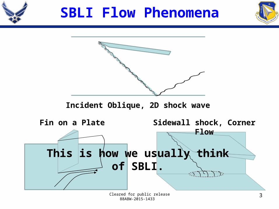
SBLI Flow Phenomena

This is how we usually think of SBLI.

Incident Oblique, 2D shock wave

Fin on a Plate Sidewall shock, Corner Flow


4

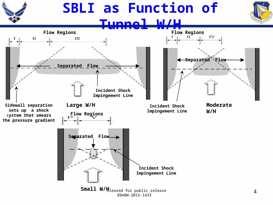
SBLI as Function of Tunnel W/H

Small W/H

Flow Regions

Separated Flow

Incident Shock Impingement Line


Moderate W/H

Separated Flow

Flow Regions

Large W/H

Flow Regions

Separated Flow


Sidewall separation sets up a shock system that

smears the pressure gradient


5

Dominant Physics

With decreasing tunnel width Corner interactions make up larger portion of flow Corner shocks change the adverse pressure gradient

Affect the character of the SBLI and separated regions Magnitude of effects depend on size of boundary layer

Hypothesis:Separation zone is function of BL thickness & tunnel

width


6

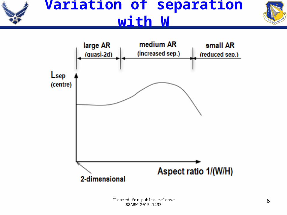
Variation of separation with W


7

Modeling and Simulation


Modeling and Simulation

8

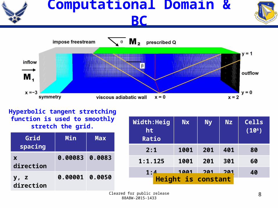
Computational Domain & BC

Hyperbolic tangent stretching function is used to smoothly stretch

the grid.Width:Height

RatioNx Ny Nz Cells

(106)

2:1 1001 201 401 80

1:1.125 1001 201 301 60

1:4 1001 201 201 40

Grid spacing Min Max

x direction 0.00083 0.0083

y, z direction 0.00001 0.0050

Height is constant


9

Code and Turbulence Models

OVERFLOW: VERSION 2.2g 16 August 2013 Non-equilibrium k-w (Hamlington and Dahm) model Quadratic Constitutive Relation (QCR) CNL1=0.3

Standard k-w

Non-equilibrium k-wCleared for public release

88ABW-2015-1433

QCR

10

Solver and Flow Parameters

2nd order Central difference flux scheme (IRHS=0 FSO=2) DDADI algorithm (ILHS=3) 2nd order HLLC flux scheme (IRHS=5 FSO=2) SSOR algorithm (ILHS=6) Local time stepping (ITIME=1) Koren limiter (ILIMIT=1)


11

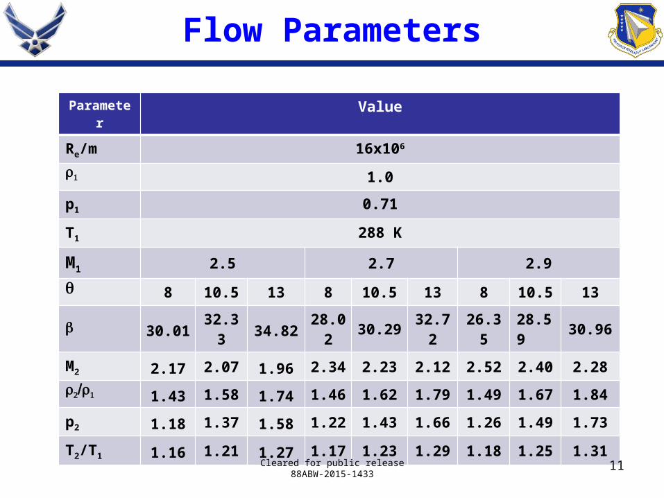
Flow Parameters

Parameter Value

Re/m 16x106

r1 1.0

p1 0.71

T1 288 K

M1 2.5 2.7 2.9

q 8 10.5 13 8 10.5 13 8 10.5 13

b 30.01 32.33 34.82 28.02 30.29 32.72 26.35 28.59 30.96

M2 2.17 2.07 1.96 2.34 2.23 2.12 2.52 2.40 2.28

r2/r1 1.43 1.58 1.74 1.46 1.62 1.79 1.49 1.67 1.84

p2 1.18 1.37 1.58 1.22 1.43 1.66 1.26 1.49 1.73

T2/T1 1.16 1.21 1.27 1.17 1.23 1.29 1.18 1.25 1.31


12

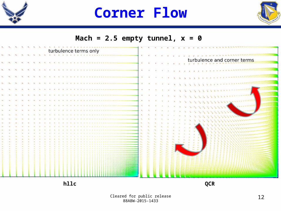
Corner Flow


hllc QCR

Mach = 2.5 empty tunnel, x = 0

13

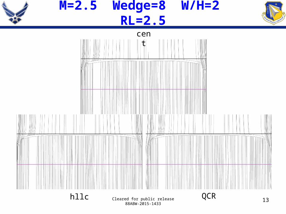
M=2.5 Wedge=8 W/H=2 RL=2.5

hllc QCRCleared for public release88ABW-2015-1433

cent

14

M=2.5 Wedge=8 W/H=2 RL=5.5

hllc With QCRCleared for public release88ABW-2015-1433

cent

15

M=2.9 Wedge=13 W/H=2 RL=2.5


cent

16

M=2.9 Wedge=13 W/H=2 RL=5.5


cent

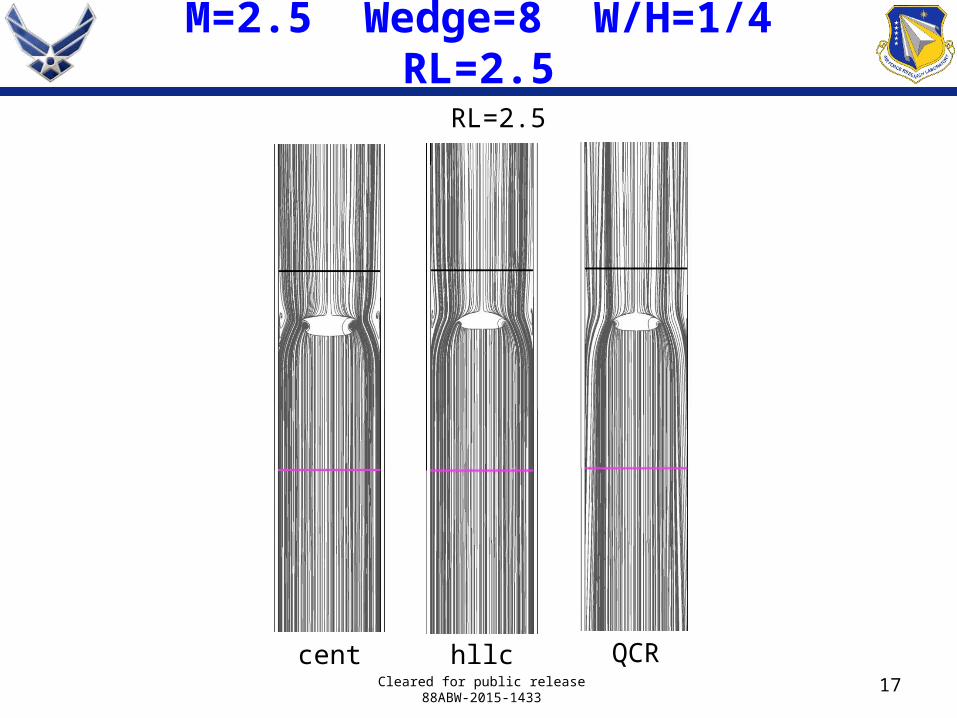
M=2.5 Wedge=8 W/H=1/4 RL=2.5

17

hllc

RL=2.5


QCRcent

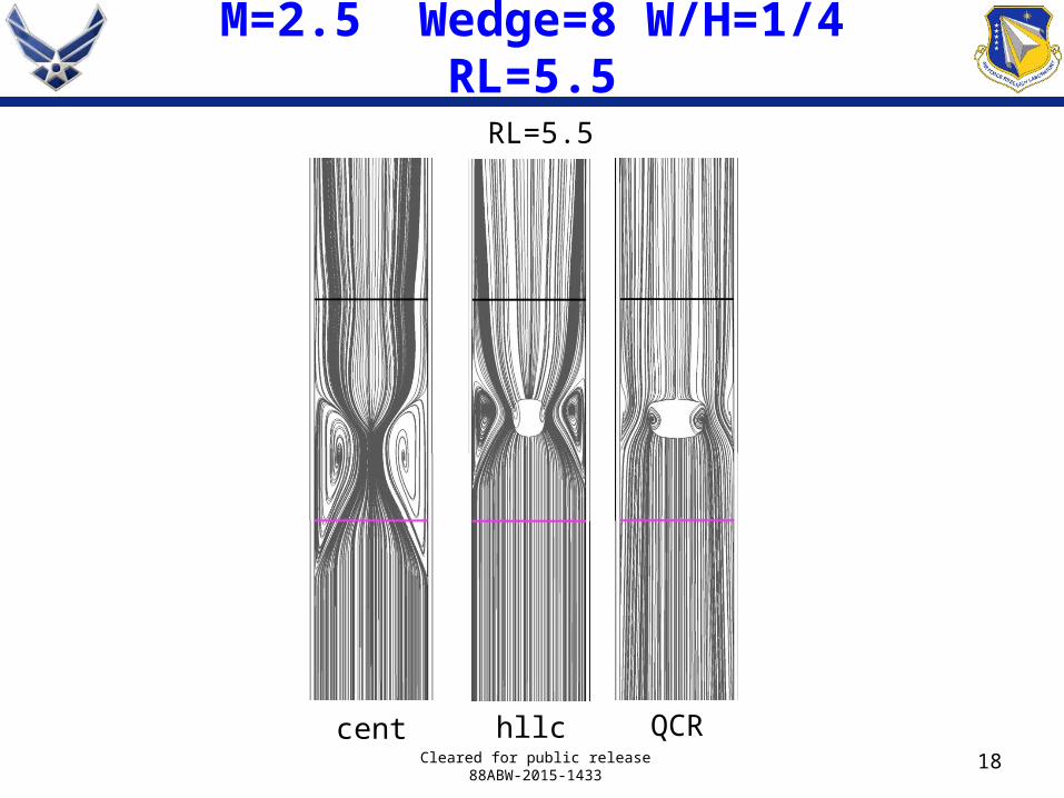
M=2.5 Wedge=8 W/H=1/4 RL=5.5

18

RL=5.5


hllc QCRcent

19

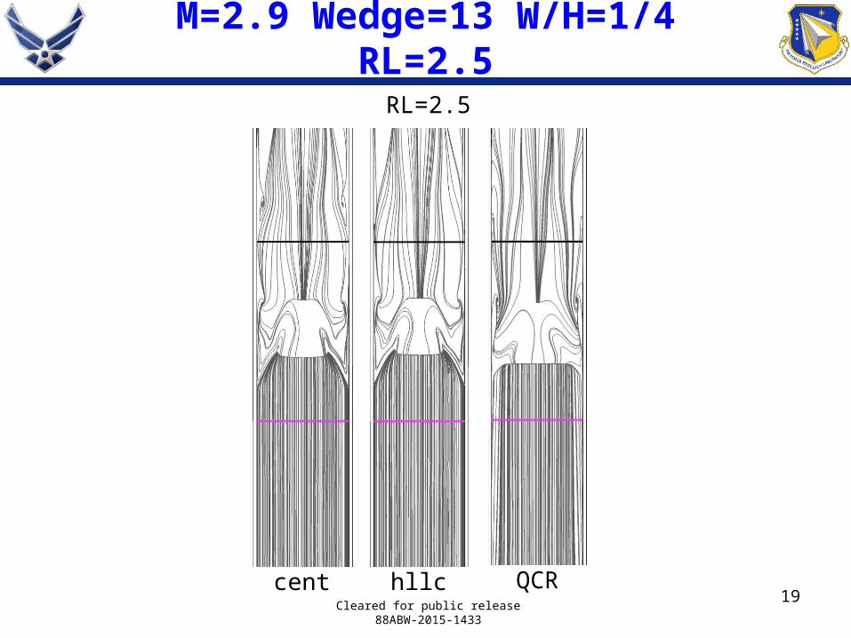
M=2.9 Wedge=13 W/H=1/4 RL=2.5


RL=2.5

hllc QCRcent

20

M=2.9 Wedge=13 W/H=1/4 RL=5.5


RL=5.5

cent hllc QCR

M=2.5 Wedge=8 W/H=2 RL=2.5

21

Inviscid flow incident shock impingement line


x=0

hllc

QCR

x=0

x=-1/2

x=-1/2

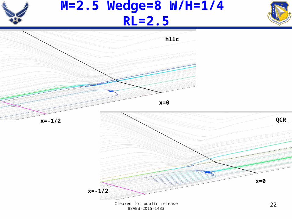
M=2.5 Wedge=8 W/H=1/4 RL=2.5

22Cleared for public release88ABW-2015-1433

x=0

hllc

QCR

x=0

x=-1/2

x=-1/2

M=2.9 Wedge=13 W/H=2 RL=2.5


x=0

hllc

QCR

x=0x=-1/2

x=-1/2

M=2.9 Wedge=13 W/H=1/4 RL=2.5


x=0

hllc

QCR

x=0

x=-1/2

x=-1/2

M=2.5 Wedge=8 W/H=2 RL=2.5

25

Isosurface ∂xr

planes ∂xrhllc

QCRCleared for public release

88ABW-2015-1433

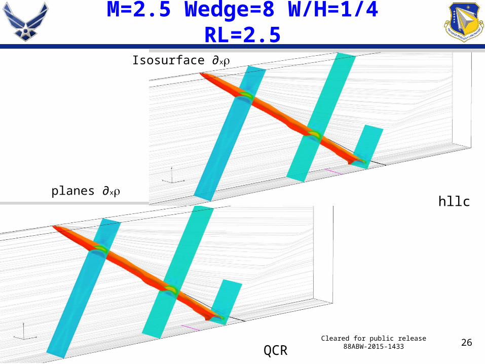
M=2.5 Wedge=8 W/H=1/4 RL=2.5

26

Isosurface ∂xr

planes ∂xrhllc


88ABW-2015-1433

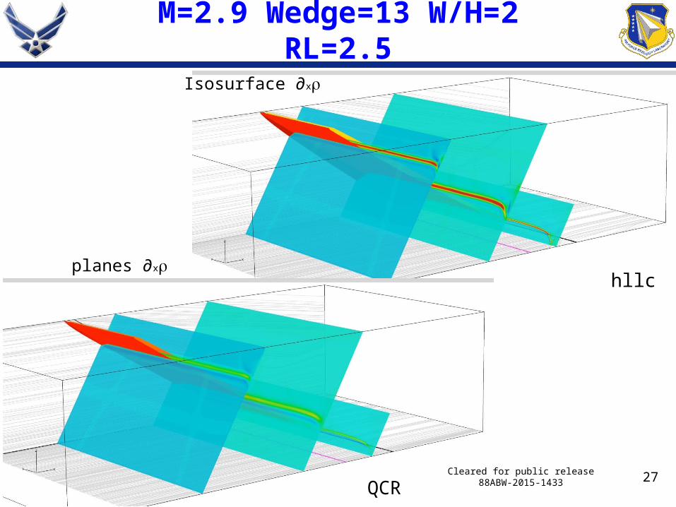
M=2.9 Wedge=13 W/H=2 RL=2.5

27

Isosurface ∂xr

planes ∂xrhllc


88ABW-2015-1433

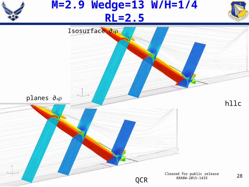
M=2.9 Wedge=13 W/H=1/4 RL=2.5

28

Isosurface ∂xr

planes ∂xrhllc


88ABW-2015-1433

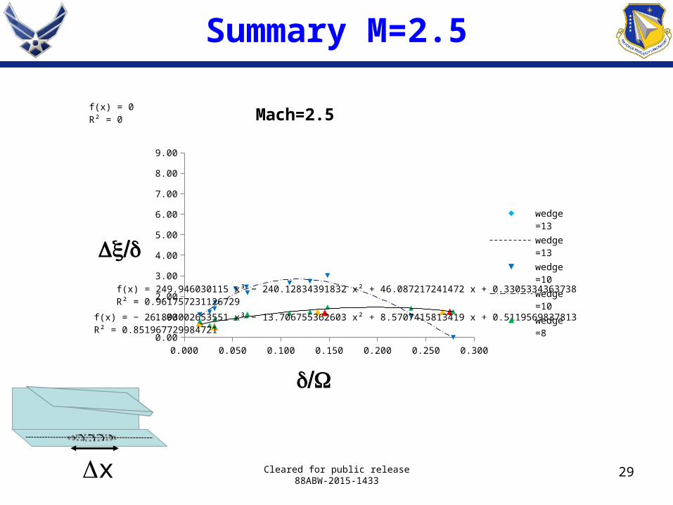
Summary M=2.5


0.000 0.050 0.100 0.150 0.200 0.250 0.3000.00

1.00

2.00

3.00

4.00

5.00

6.00

7.00

8.00

9.00

f(x) = − 26.893002653551 x³ − 13.7067553626034 x² + 8.57074158134192 x + 0.511956983781272R² = 0.851967729984721

f(x) = 249.946030114997 x³ − 240.128343918322 x² + 46.0872172414717 x + 0.330533436373778R² = 0.961757231126729

f(x) = 0R² = 0 Mach=2.5

wedge=13wedge=13wedge=10wedge=10wedge=8wedge=8

/d W

/Dx d

Dx

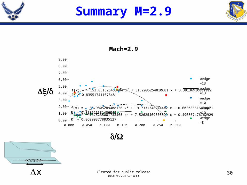
Summary M=2.9

30Dx Cleared for public release88ABW-2015-1433

0.000 0.050 0.100 0.150 0.200 0.250 0.3000.00

1.00

2.00

3.00

4.00

5.00

6.00

7.00

8.00

9.00

f(x) = − 16.8235001733465 x² + 7.52625469308899 x + 0.49686747676293R² = 0.860993778835127

f(x) = − 55.9305289408136 x² + 19.7331348944402 x + 0.603085516650071R² = 0.853625531406843

f(x) = − 153.851525453484 x² + 31.2095254810681 x + 3.38136910882912R² = 0.83551741107848

Mach=2.9

wedge=13wedge=13wedge=10wedge=10wedge=8wedge=8

/d W

/Dx d

31

Design of Experiments

Determine the range of input parameters and the outputs to be modeled.

Create a list (matrix) of simulations to run. Run the simulations (this is the long part). Fill in matrix with outputs. Run software to determine sensitivities. Create response surface.


32

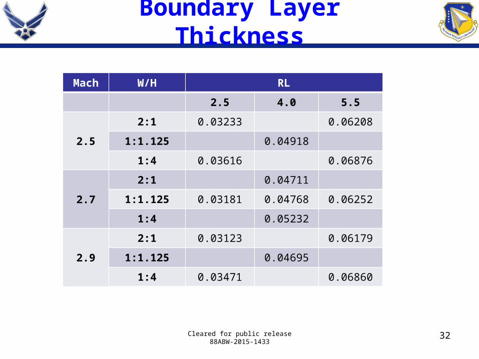
Boundary Layer Thickness


Mach W/H RL

2.5 4.0 5.5

2.5

2:1 0.03233 0.06208

1:1.125 0.04918

1:4 0.03616 0.06876

2.7

2:1 0.04711

1:1.125 0.03181 0.04768 0.06252

1:4 0.05232

2.9

2:1 0.03123 0.06179

1:1.125 0.04695

1:4 0.03471 0.06860

33

DoE Boundary Layer Thickness

Three input parametersMach numberTunnel WidthRun Length, RL

Most sensitive to RL Least sensitive to Mach number Response surface is a good fit to data


34

DoE Separation Length

Four input parameterMach numberWedge angle, qTunnel WidthRun Length, RL

Exploring polynomial response surfaces


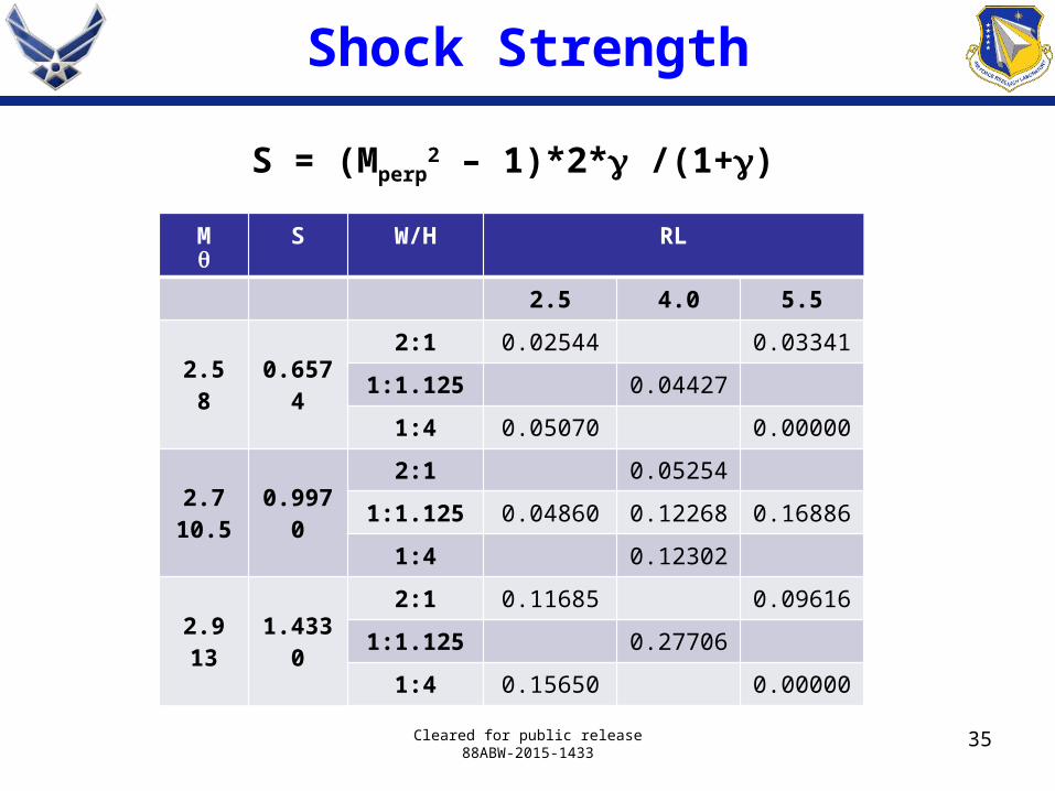
35

Shock Strength


Mq

S W/H RL

2.5 4.0 5.5

2.58 0.6574

2:1 0.02544 0.03341

1:1.125 0.04427

1:4 0.05070 0.00000

2.710.5 0.9970

2:1 0.05254

1:1.125 0.04860 0.12268 0.16886

1:4 0.12302

2.913 1.4330

2:1 0.11685 0.09616

1:1.125 0.27706

1:4 0.15650 0.00000

S = (Mperp2 – 1)*2*g /(1+g)

36

Future Work

Compare Dahm to k-w Further investigation with DoE Fill in our Summary curves Effect on interactions of Height Acquire x/ vs /W from literature and

compare with computations Experiments in Cambridge

corner flow suction/blowing


investigations of wind tunnel size and shock strength on shock boundary layer interactions john a....

Documents

public release

qcr slide

cent slide

simulation slide

corner flow

small wh flow regions

hllc qcr

hllc rl