TaxFACTs Schriftenreihe Nr. 2011-05

Investment and Firm-Specific Cost of Capital:Evidence from Firm-Level Panel Data

Thiess Buettner(FAU and CESifo)1 2

Anja Hoenig(FAU)

December 2011

Abstract: To study the effects of taxes on investment, this paper employs a novel firm-level

dataset of German manufacturing companies which combines survey data with financial accounts.

The information enables us to construct indicators of the cost of capital which capture the specific

conditions of each firm including its location as well as asset and capital structures. Our results

indicate that, in order to identify tax effects, it is important to take this firm-specific variation into

account. In particular, accounting for the firms’ capital structure is found to be crucial; ignoring

this variation would result in insignificant tax effects and specification problems.

Keywords: Cost of Capital; Investment; Capital Structure; Firm-Level Data; Survey Data; Local

Business Tax; Business Expectations; GMM

JEL Classification: H25, H32, H73

1Address: Friedrich-Alexander-University (FAU)Lange Gasse 20D-90403 NurembergGermany

Phone:Fax:E-mail:

+49 911 5302 200+49 911 5302 396thiess.buettner@wiso.uni-erlangen.de

2For comments on an earlier draft we are indebted to Martin Falk, Simon Loretz, Joachim Winter, and participants

at conferences and seminars in Uppsala, Munich, and Mannheim.

Kommunikation

TaxFACTs – Forschungsschwerpunkt SteuernFriedrich-Alexander-Universitat Erlangen-Nurnberg

Lange Gasse 2090403 Nurnberg, Germany

Tel.: +49 911 5302-376Fax: +49 911 5302-428E-Mail: info@steuerinstitut-nuernberg.de

1 Introduction

The adverse effects of corporate taxation on investment and the stock of capital are key issues

in academic and public debates about tax policy. While empirical research generally supports

significant effects, the available evidence differs with regard to the strength of the influence (surveys

are provided by Chirinko, 2002, and Hubbard and Hassett, 2002). A larger literature shows that

providing empirical evidence about how changes in taxes affect investment and the stock of capital

has proved to be rather difficult. With regard to investment, research could take advantage of

the immediate effects of tax changes on the value of firms, and studies relying on the q-theory

of investment have detected substantial tax effects (e.g., Cummins, Hassett, and Hubbard, 1994).

Regarding the effects on the capital stock, however, most research has found only small effects. The

dominant approach taken in the literature is concerned with the effects of the cost of capital on

investment. Macroeconomic research following the so-called neoclassical approach using time-series

data faces a host of problems such as simultaneity and aggregation biases. But also studies using

firm-level data often find only small effects (e.g., Chirinko, Fazzari, and Meyer, 1999). While the

approach relying on the cost of capital has the advantage that relevant parameters associated with

corporate taxation can be included such as the statutory tax rate, tax-depreciation allowances and

special tax incentives, empirical research indicates that it is difficult to find sufficient institutional

variation. This is a problem in particular in the context of domestic firms that are subject to the

same tax law – in contrast to multinational firms that operate in different countries.

Even if the same tax law applies to all firms, it is well known that the tax system treats firms

differently. For instance, different types of assets like buildings or machinery are taxed differently

due to differences in depreciation allowances. Moreover, corporate tax systems usually discriminate

between different sources of finance. As a consequence, the cost of capital differs across firms

and also reforms in the tax system, which introduce exogenous variation in key tax parameters,

are influencing firms differently. To explore the research opportunities that arise from the firms’

heterogeneity with regard to asset and capital structures, this paper employs a novel firm-level

dataset of German manufacturing companies which enables us to compute firm-specific indicators

of the cost of capital. The institutional setting in Germany provides us with further opportunities

1

to identify tax effects since the local business tax varies at the level of municipalities. Furthermore,

with data covering the period 1994-2007 we can exploit major institutional changes in the tax law.

The results support the importance of using firm-specific variation for identifying tax effects. Our

key finding is that GMM estimation of a partial adjustment model which takes account of firm-

specific differences yields a significant cost of capital elasticity of the stock of capital of about unity

of larger (in absolute terms). However, ignoring firm-specific variation results in weaker tax effects

and is associated with specification problems.

The paper is organized as follows. In Section 2 we derive the firm-specific measure of the cost

of capital and discuss how to implement it empirically. Dataset and investigation approach are

discussed in Section 3. Section 4 provides results using a distributed lag model, which has often

been used in the literature. Section 5 reports results obtained from a GMM approach that is

particularly suited to exploit the opportunities arising from panel data. In Section 6 we finally

explore the role of the firm-specific variation by abstracting from the local variation in the business

tax rate and fixing capital and asset structures. Finally, Section 7 provides a brief summary and

concludes.

2 Investment and Firm-Specific Cost of Capital

To capture the role of taxation for company investment, we follow the cost of capital approach dating

back to Jorgenson (1963), Hall and Jorgenson (1967), and King (1974), and further developed by

Devereux and Griffith (1998, 2003). This approach is based on the view that a capital stock is

optimal if the effect of a marginal addition to the capital stock on the firm value is zero. Before

deriving a firm-specific indicator of the cost of capital, the following subsection briefly discusses the

determination of the firm value.

Basic Model of Firm Value As usual, we derive the firm value Vt at the end of period t by

considering the arbitrage equilibrium condition between investment in the firm’s equity relative

2

to investment in some alternative asset with a fixed rate of interest. Following Devereux (2004),

abstracting from shareholder taxation, the arbitrage equilibrium condition can be specified as

(1 + r)Vt =1

1− cDt+1 + Vt+1, (1)

where r is the nominal rate of return on a risk-free asset and Dt+1 denotes dividend payments. c

captures a tax credit for profit distribution. More precisely, c is the corporation tax rebatement

expressed as a fraction of dividends.1 According to equation (1), at the end of period t + 1, the

return from lending in the amount of Vt (left hand side) is required to be equal to the payoff from

an investment in equity (right hand side), the latter consisting of dividend payments and a change

in firm value. We could also take account of new share issues in the definition of the firm value.

But, since we abstract from the taxation at the level of shareholder it is not meaningful to discuss

the discrimination of the tax system with regard to new equity.

Assuming that the firm value is bounded,2 repeated substitution enables us to solve for the firm

value as a present value of dividends

Vt =γ

1 + r

(Dt+1 +

1

1 + rDt+2 +

(1

1 + r

)2

Dt+3 + ...

), (2)

where the parameter γ ≡ 1(1−c) captures the tax advantage of distributing profits relative to retain-

ing profits which arises from the presence of the dividend tax credit. Dividend payments obey

Dt+1 = (1− τ) (1 + π)F (Kt)− qt+1It+1 +Bt+1 − (1 + (1− τ) r)Bt + τϕ(qt+1It+1 +KT

t

). (3)

Here, F (Kt) is output in period t + 1 depending on the existing capital stock Kt, τ reflects the

statutory tax rate, π is the (general) inflation rate relative to the current output price pt, which

is set to unity, for simplicity. It+1 is investment, Bt is the existing stock of debt served at the

common rate of interest r and Bt+1 is the stock of debt at the end of the period t+ 1. ϕ is the

1This captures a specialty of the German corporation tax (see McDonald, 2001, for a discussion), which has been

abolished in 2001, however.

2Formally, limT→∞.

(1

1+r

)T−tVT = 0

3

capital allowance rate capturing tax depreciation allowances and KTt is the tax accounting value of

the capital stock defined as

KTt = (1− ϕ)qt−1It−1 + (1− ϕ)KT

t−1 = (1− ϕ) qt−1It−1 + (1− ϕ)2 qt−2It−2 + ... (4)

qt is the price of the capital good increasing each period according to the inflation rate πI such

that qt+1 = (1 +πI)qt. Similar to the output price, qt is set to unity. The accumulation equation is

Kt+1 = (1− δ)Kt + It+1 (5)

where δ is the rate of economic depreciation.

Cost of Capital with Retained Earnings To derive the cost of capital we follow Devereux

(2004) and consider a hypothetical investment increasing the capital stock by one unit in period

t and assume that the company’s general purpose is the maximization of the firm value, i.e. the

market value Vt. The optimal capital stock can be found using equations (1) to (5) and setting

∂Vt/∂Kt+1 = 0. As a result, we get the first order condition

(1− τ) (1 + π)F ′ (Kt+1) = (1−A)(r + δ(1 + πI)− πI)

)reflecting that, in the optimum, the after-tax value of output (left hand side) in period t + 1 is

equal to the cost of increasing Kt. A is the net present value of allowances if declining-balance

depreciation is applied,3 with

A ≡ τϕ(1 + r)

ϕ+ r. (6)

Obviously, the first order condition does not allow for changes in debt or new equity finance.

Instead, it is implicitly assumed that the unit increase of the capital stock is financed by a reduction

in dividends, i.e. by retained earnings. The cost of capital, defined as the minimum acceptable

3The present value of depreciation allowances depends on the type of asset, the respective depreciation rate and

allowance scheme. In the case of straight-line depreciation, A ≡ τϕ(1+r)r

(1 − 1(1+r)n

) where n is the number of years

for which depreciation allowances can be claimed. For more information, see also the Appendix.

4

pre-tax rate of return, is

cocRE ≡ (1−A)

(1− τ) (1 + π)

(r + δ

(1 + πI

)− πI

)− δ. (7)

Cost of Capital and the Firm’s Capital Structure While we have assumed so far that the

marginal source of finance is retained earnings, let us augment the model to include debt as an

additional source of financing. If the firm uses debt finance, it benefits from the deductibility of

interest payments in determining corporate profits. As a consequence, the cost of capital tends to

be lower with debt finance. While this seems to suggest that the most tax efficient way to finance

investment is to rely exclusively on debt finance, the corporate finance literature emphasizes non-

tax determinants of capital structure choice. Due to information asymmetries, debt finance can

play an important role in reducing incentive problems associated with the management of the firm

(Aghion and Bolton, 1989). In a similar vein, Jensen (1986) argues that debt might be helpful

to reduce disincentives associated with free cash flow. Moreover, debt finance is associated with

agency cost due to potential conflicts between equity and debt claimants (e.g., Jensen and Meckling,

1976; Myers, 1977). To take these considerations into account, we might assume that each firm

has a specific target value for the share of debt based on incentive considerations alone. Let us

specify this target level with λ. If deviating from this target value is associated with costs, optimal

investment finance will trade off the tax-advantage from using more debt against the costs associated

with distorting the capital structure (Huizinga, Laeven, Nicodeme, 2006). For simplicity, one might

assume that the cost of deviating from the optimal mix of financing with debt and retained earnings

is very high. With this assumption, an investment project will be financed usually with a ratio of

debt to capital that is consistent with the target level λ. If the cost of deviating from the preferred

capital structure is less than prohibitive, the actual share of debt used to finance investment is

determined by a function Λ (λ,∆), which is increasing in the preferred debt-to-capital ratio λ as

well as in the tax-advantage of using debt, denoted with ∆, which is derived below.

With a share Λ of investment being financed with new debt and only a share 1−Λ being financed

with retained earnings, the cost of capital will differ from the base case analyzed above. The

derivation of the cost of capital with debt finance is the same, except that we have to consider an

5

increase in borrowing during the investment period (see (3)). Note that we follow Devereux (2004)

and assume that debt is increased only temporarily and repaid after one period. With a share of

debt finance Λ, the adverse effect of investment on dividends is reduced

∂Dt

∂Kt+1= −qt (1− τϕ) (1− Λ) .

In the second period, however, dividends decline since debt obligations are served and repaid.

∂Dt+1

∂Kt+1= − (1 + (1− τ) r) (1− τϕ) qtΛ.

Taking these additional effects into account in the derivation, we can specify the cost of capital

with a share Λ of debt finance as:

coc ≡ cocRE − Λ(1− τϕ) (rτ)

(1− τ) (1 + π)︸ ︷︷ ︸∆

, (8)

where ∆ is the difference between the cost of capital entirely using retained earnings and entirely

relying on debt finance. As already noted, if the cost of deviating from the preferred capital

structure is less than prohibitive, the actual share of debt used to finance investment is a function

Λ (λ,∆) of the preferred debt-to-capital ratio and the differential cost of capital ∆. This has some

implications for the empirical analysis, which are further discussed below.

Cost of Capital and the Firm’s Asset Structure To further take account of differences in

the investment projects undertaken and to be able to calculate tax-depreciation allowances for

each firm, we also consider a company’s asset structure. While we do not have information about

actual investment project’s characteristics, we aim at capturing differences related to the firm-

specific characteristics of the production process. Taking three types of assets into account, namely

industrial buildings (B), plant/ machinery (M) and inventories (STO), we construct weights Ω for

6

each firm with ΩB + ΩM + ΩSTO = 1:

ΩB =B

B +M + STO

ΩM =M

B +M + STO

ΩSTO =STO

B +M + STO

We use these weights to calculate firm-specific depreciation rates δ, firm-specific rates of capital

allowances ψ and net present values of allowances, A, depending on both asset-specific depreciation

rates and allowance schemes:

δ = δBΩB + δMΩM + δSTOΩSTO

ψ = ψBΩB + ψMΩM + ψSTOΩSTO

A = ABΩB +AMΩM +ASTOΩSTO.

Not only in the case of the capital structure, but also with regard to asset structures, differences in

the tax treatment might exert some distortions. This would suggest that the shares ΩB ΩM , and

ΩSTO, might be correlated with the differential tax effects AB, AB, and ASTO.

3 Data and Investigation Approach

The empirical analysis employs an unbalanced panel of matched survey and financial statement

data which focuses on German firms and covers the period 1994-2007. Institutional details and tax

parameters including the tax rate at each firm’s location are used to calculate the cost of capital

as outlined in the previous section. The survey data stems from the manufacturing sector of the

monthly ifo Business Survey and allows us to control for a firm’s business expectations (commercial

expectations) or current business situation (state of business). This information is captured by

ordinal variables, where a value of 1 indicates an ‘improved/improving’ situation or expectations,

0 means ‘unchanged/unchanging’ and −1 reflects a ‘deteriorated/deteriorating’ assessment. To

account for differences between firms’ current business situations, we include indicators of the state

7

of business or the business expectations at the time of investment planning, i.e. during the last 6

months preceding the investment period.

In total, there are about 8000 observations based on 1835 firms in the dataset but only for about

2300 observations information on all required covariates and instrumental variables is available for

our preferred specification. Table (1) provides some descriptive statistics for our sample containing

unweighted annual averages of the variables employed.4 Obviously, sales and asset figures indicate

a period of growth during the 1990s and a weaker performance in the subsequent period after the

introduction of the Euro and the so called ‘dot-com’ bubble. From 2004 onwards, there are more

companies and thus more balance sheets included in the underlying financial statement data.5

To compute the cost of capital we follow Devereux and Griffith (1999, 2003) and Yoo (2003), and

fix the rate of economic depreciation at δM = 12.25% for machinery, δB = 3.61% for buildings and

δSTO = 0% for inventories, as these are not depreciable.6 Depreciation rates for tax purposes, i.e.

capital allowances for industrial buildings, machinery and inventory are computed following the tax

law. As in the study by Yoo (2003) and Devereux et al. (2008) we take account of both allowance

rates and information on the taxation-relevant lifetime of an asset. With regard to the net present

value of depreciation allowances we follow German tax law and use straight-line depreciation for

buildings and the declining-balance method for machinery. Furthermore, the tax rate τ in equation

(8) is the year-specific statutory tax rate on retained earnings, including the corporation tax, the

solidarity surcharge as well as the local business tax. The latter is taken into account separately

for each firm and year and depends on a firm’s location in Germany. Some more details on the tax

system and recent reforms are given in the Appendix. To compute the user cost of capital given

in (8) we take annual data on nominal interest and inflation rates.7 Exploiting the micro-level

4We measure investment and the capital stock by tangible assets. For further information on the dataset used see

the Appendix and Hoenig (2010).

5When the dataset was established, most of the balance-sheets for the year 2007 were not yet available such that

the number of observations in our sample drops again in 2007.

6According to tax law, we apply the LIFO method to valuate inventory.

7Information on nominal interest rates is taken from the German Council of Economic Experts, inflation rates are

based on the yearly consumer price index of the Federal Statistical Office. In this respect, the inflation rate of output

is set equal to the inflation rate in the capital stock.

8

Tab

le1:

SummaryStatisticsofFirm

Variables

1995

1996

1997

1998

1999

2000

2001

Tan

gib

leas

sets

(Mil

l.E

UR

)96.5

6104.6

2103.1

5112.6

0113.3

5108.7

374.7

9(2

81.1

7)

(292.8

3)

(299.5

1)

(311.8

0)

(307.0

7)

(325.2

9)

(125.4

2)

Sal

es(M

ill.

EU

R)

762.8

9810.8

5873.7

4936.0

9849.0

9650.5

9473.9

4(2

713.5

9)

(2840.3

0)

(3164.3

6)

(3403.0

8)

(3173.8

1)

(1805.6

0)

(802.1

8)

Cos

tof

Cap

ital

.097

.092

.073

.077

.075

.076

.045

(.019)

(.015)

(.012)

(.011)

(.010)

(.011)

(.006)

Sta

teof

bu

sines

s-.

004

-.184

.051

.049

.015

.192

-.065

(.554)

(.517)

(.565)

(.546)

(.541)

(.548)

(.506)

Com

mer

cial

exp

ecta

tion

s-.

042

.021

.132

.042

.058

.096

-.130

(.395)

(.412)

(.396)

(.383)

(.395)

(.394)

(.415)

Nu

mb

erof

obse

rvat

ion

s173

176

163

157

164

152

140

2002

2003

2004

2005

2006

2007

Tan

gib

leas

sets

(Mil

l.E

UR

)65.3

793.3

874.0

565.7

158.5

890.9

0(9

2.8

8)

(304.6

7)

(274.2

5)

(244.4

2)

(221.0

9)

(312.6

1)

Sal

es(M

ill.

EU

R)

479.2

7635.1

3507.9

3466.0

3439.0

3710.0

7(8

34.2

4)

(1916.2

7)

(1827.8

1)

(1732.4

7)

(1826.5

5)

(2572.5

6)

Cos

tof

Cap

ital

.050

.047

.034

.031

.036

.035

(.006)

(.006)

(.006)

(.005)

(.006)

(.006)

Sta

teof

bu

sines

s-.

238

-.122

.059

.043

.307

.401

(.506)

(.545)

(.537)

(.555)

(.574)

(.557)

Com

mer

cial

exp

ecta

tion

s.0

26

.121

.076

.068

.090

.104

(.421)

(.426)

(.442)

(.387)

(.388)

(.371)

Nu

mb

erof

obse

rvat

ion

s138

172

197

260

310

187

All

valu

esre

pre

sent

unw

eighte

dav

erages

,st

andard

dev

iati

ons

inpare

nth

eses

.V

ari

able

sst

ate

of

busi

nes

sand

com

mer

cial

exp

ecta

tions

refe

ronly

toth

ese

cond

half

of

the

yea

r.

9

information in our dataset which reports each company’s capital structure in the financial account

statements we are able to compute a firm-specific, time-varying measure of Λ.8

With regard to the cost of capital, the figures emphasize the consequences of the 2001 tax reform

which was intended to improve the German position in international tax competition by lowering

the statutory tax rate at the company level. Since an important part of the tax burden originates in

the local business tax, the cost of capital displays substantial variation across space (see Figure 1).

Considering average sales, rather large companies seem to be included in the sample. Nevertheless,

the annual median value of sales makes up some 20 % of the annual mean. This points at a skewed

distribution which is also reflected by the large standard deviations.

While the cost of capital captures both the local business tax and federal taxes as well their

interaction, it does not take account of some specific features of the local business tax. Although this

tax is primarily levied on profits, there are important additions to the tax base, in particular, 50%

of long-term interest is added.9 This element of the tax might exert effects on the choice between

different sources of finance. A second important element is that for multiregional corporations with

branches and/or subsidiaries in different locations, there is formula apportionment based on the

payroll. As is well known from the theoretical literature on formula apportionment (Gordon and

Wilson, 1986), such institutions alter the nature of the tax and, at least partially, the tax becomes

a tax on the formula weights. With payroll as formula weight, we should expect that high tax

rates provide incentives to substitute labor with other inputs and factors such as capital. To take

account of this effect we test for a separate impact of an index that captures this incentive. The

details of the computation of this index are provided in the Appendix.

The starting point to derive a useful specification for our empirical investigation is a neoclassical

production function with capital and labor as inputs to production. Assuming perfect competition,

we can easily derive the first order condition for the optimal capital stock to get a static log-linear

8Λ is defined as the share of debt to total capital with debt being interest-bearing debt and total capital being

the sum of nominal capital, capital and profit reserves as well as total debt.

9In 2008, which is not included in our estimation sample, the additions have been changed by a major tax reform.

10

Figure 1: Cost of Capital in 2006

Map plots the cost of capital for an investment financed with retained earnings using average values for the debt-to-

capital ratio and the asset structure. White spots refer to missing data.

11

relationship between the capital stock, the output and the cost of capital of a company

K?t ≡ κσYtcoc−σt ,

where σ is the elasticity of substitution between labor and capital. If investment projects take

more than one period in order to be realized, however, investment will be spread over multiple

periods and a firm’s capital stock deviates from its optimal level. The literature in the tradition of

Jorgenson (1963), therefore, explains the current capital stock by a sequence of terms

lnKt =n∑i=0

wi [lnYt−i − σcoct−i] .

In order to remove time-invariant determinants and to facilitate the measurement of determinants

of output and the user cost, much of the literature uses a first differenced version of this equation.

Taking account of possible differences in the effects of output and cost of capital, the literature (see

Chirinko, 1993) employs a function

∆ lnKt =n∑i=0

αi∆ lnYt−i +n∑i=0

θi∆ ln coct−i + εt, (9)

where the change in the stock of capital (in logs) with regard to the previous period is the dependent

variable. If lag-length is chosen correctly, autocorrelation is no longer present and estimation is

carried out using OLS or, perhaps, using IV approaches to control for possible simultaneity biases

with regard to the contemporaneous variables.

With micro-level panel data and depending on the adjustment cost function, it seems a bold attempt

to include a number of lags of explanatory variables that is sufficient to remove all autocorrelation.

If the available time span is limited10, however, as is usually the case with firm level panel data,

an alternative and perhaps more appropriate approach is to employ a partial adjustment model

that explicitly takes account of first-order autocorrelation and avoids using higher order lags of

explanatory variables

∆ln(Kt) = ρln(Kt−1) + αln(Yt) + θln(coct). (10)

10See Dwenger (2010) for an approach that combines ADL and partial adjustment models.

12

Taking a firm’s sales as our output variable Yi,t and including the firm-specific cost of capital as

specified in section (2) along with further relevant variables, the regression equation becomes:

ln(Ki,t) = (1 + ρ)ln(Ki,t−1) + αln(Yi,t) + βcomexi,t + θln(coci,t) + φt + ui,t,

ui,t = ηi + εi,t

(11)

where ln(Ki,t) is the capital stock of firm i in year t. Here, the coefficient (1 + ρ) on the lagged

capital stock ln(Ki,t−1) reflects the adjustment process triggered by current investment. As already

mentioned, beyond a firm’s sales and capital cost we include a firm’s appraisal of its actual state

of business (stbi,t) at the beginning of year t. Similarly, in an alternative setting, we include the

firm’s commercial expectations (comexi,t) measured as the average expectation of firm i over the

second half of period t − 1. Furthermore, to control for time effects common to all firms and to

capture cyclical productivity or price-level shocks, equation (11) includes period-specific intercepts

φt. In addition, the error term ui,t contains ηi, denoting a firm-specific fixed effect controlling for

unobservable company characteristics, and εi,t, which is the remaining disturbance term.

From an econometric point of view, the specification in equation (11) faces problems of simultaneity

and endogeneity as the contemporaneous cost of capital and sales variables are possibly correlated

with the error term. Moreover, the inclusion of the lagged dependent variable results in the well-

known dynamic panel bias in the presence of time-invariant firm-specific fixed effects (see Nickell,

1981). Since a simple fixed effect estimation may yield biased and inconsistent estimates, we utilize

a Generalized Method of Moments (GMM) estimator. This estimator allows us to handle not only

the dynamic structure of the model and predetermined or endogenous explanatory variables, but

also firm-specific factors, heteroskedasticity, and autocorrelation of individual observations. More

specifically, we employ the system GMM estimator outlined by Arellano and Bover (1995) and

refined by Blundell and Bond (1998) since it alleviates some of the shortcomings of the Arrelano-

Bond (1991) first-difference GMM estimator, if applied to autoregressive models for moderately

persistent series in short panels.11

11Some difficulties in application of the difference GMM estimator are mentioned in Blundell and Bond (1998),

Beck, Levine and Loayza (2000) or Griliches and Hausman (1986). To implement the system GMM estimator we use

the xtabond2 command in STATA introduced by Roodman (2006).

13

4 Results of the Distributed Lag Model

Taking the existing literature as a point of departure, we follow Chirinko, Fazzari and Meyer

(1999) and start with the distributed lag model (9) to estimate the relationship between taxation

and company investment. Table 2 provides some basic results for different numbers of lags. In this

model, the response of the capital stock to changes in the firm-specific cost of capital is captured

by the sum of coefficients.

Though the coefficient of determination tends to increase with the inclusion of higher order lags, the

results of specifications with more than one or two lags are somewhat disappointing. While the sales

variable judged on basis of the sum of coefficients proves significant throughout all specifications,

the cost of capital variable shows only small and often insignificant effects.

Table 3 provides some further results of specifications including fixed time effects (see DL4b) and/or

utilizing instrumental variables (see DL5a and DL5b), which may take account of possible simul-

taneity biases. Following Chirinko et al. (1999) we use twice lagged levels of variables as instru-

ments in this first-differenced equation. However, the number of observations gets very small and

the standard errors become large.

5 Results of the Dynamic Panel Data Model

As already mentioned, and in contrast to the estimators used in the traditional literature, GMM

estimation seems preferable as this allows us to take account of autocorrelation explicitly and to

handle the endogeneity of the variables while allowing for firm-specific factors. To eliminate the

time-invariant firm effects and exclude any bias potentially arising from unobserved heterogeneity,

equation (11) is first transformed into differences:

∆ln(Ki,t) = (1 + ρ)∆ln(Ki,t−1) + α∆ln(Yi,t) + β∆comexi,t + θ∆ln(coci,t) + ∆φt + ∆ui,t. (12)

14

Table 2: Results of Distributed Lag Model using Firm-Specific Cost of Capital andFixed Effects

∆ ln(Ki,t) (DL0) (DL1) (DL2) (DL3) (DL4a)

∆ ln(Yi,t)α0 .285 (.031) ∗∗∗ .466 (.048) ∗∗∗ .442 (.062) ∗∗∗ .454 (.058) ∗∗∗ .455 (.069) ∗∗∗

α1 .193 (.043) ∗∗∗ .205 (.065) ∗∗∗ .157 (.062) ∗∗∗ .058 (.073)α2 .007 (.060) -.035 (.071) .050 (.087)α3 .038 (.070) .026 (.092)α4 -.089 (.084)SUM(α) .285 (.031) ∗∗∗ .658 (.072) ∗∗∗ .654 ( .120)∗∗∗ .537 (.158) ∗∗∗ .500 (.242) ∗∗

∆ ln(cocfsi,t)

θ0 -.047 (.032) -.064 (.039)∗ -.094 (.053)∗ -.060 (.053) -.095 (.057)∗

θ1 -.058 (.040) -.075 (.054) -.118(.067) ∗ -.095 (.077)θ2 -.024 (.058) -.086 (.072) .002 (.092)θ3 -.057 (.063) .008 (.088)θ4 .106 (.069) ∗

SUM(θ) -.047 (.032) -.122 (.063)∗ -.194 (.136) -.321 (.221) -.075 (.308)

∆stbi,tβ0 .019 (.011) ∗ .000 (.014) -.002 (.018) .021 (.018) .018 (.021)β1 -.007 (.014) -.025 (.020) -.014 (.020) -.021 (.024)β2 .001 (.018) .019 (.020) .014 (.025)β3 .002 (.017) .005 (.023)β4 .010 (.019)SUM(β) .019 (.011) ∗ -.006 (.024) -.026 (.044) .028 (.055) .027 (.083)

Observations 1731 1245 902 657 479R2 .065 .102 .086 .150 .154

Following Chirinko et al. (1999), the dependent variable is firm investment scaled by the capital stock in the previousperiod. Long-run sales and cost of capital effects are represented by the sum of coefficients outlined in the last row,respectively. The same is true for the appraisal of the state of business. OLS estimates. Time effects are ignored inthis specification. Standard errors are given in parentheses. * denotes significant at 10%; ** significant at 5%; ***at 1%.

15

Table 3: Results of Distributed Lag Model using Firm-Specific Cost of Capital andInstrumental Variables

∆ ln(Ki,t) (DL4a) (DL4b) (DL5a) (DL5b)

∆ ln(Yi,t)α0 .455 (.069) ∗∗∗ .445 (.070) ∗∗∗ .044 (.428) -1.176 (6.558)α1 .058 (.073) .099 (.073) .252 (.298) 2.070 (8.887)α2 .050 (.087) .077 (.088) .111 (.141) .838 (4.075)α3 .026 (.092) .065 (.093) -.221 (.212) .159 (1.456)α4 -.089 (.084) -.050 (.085) -.104 (.127) .813 (4.057)SUM(α) .500 (.242) ∗∗ .637 (.246) ∗∗∗ .082 (.716) 2.703 (12.792)

∆ ln(cocfsi,t)

θ0 -.095 (.057)∗ -.184 (.133) -.400(.220) ∗ -13.669 (65.512)θ1 -.095 (.077) -.213 (.156) .381 (.380) 6.582 (34.963)θ2 .002 (.092) -.016 (.148) .350 (.321) .635 (3.663)θ3 .008 (.088) -.023 (.149) .418 (.351) -2.310 (9.995)θ4 .106 (.069) ∗ .323 (.139) ∗∗ .451 (.271) ∗ -.069 (1.588)SUM(θ) -.075 (.308) -.112 (.475) 1.199 (1.189) -8.832 (38.481)

∆stbi,tβ0 .018 (.021) .026 (.021) -.036 (.046) .117 (.526)β1 -.021 (.024) -.012 (.025) -.056 (.044) -.008 (.206)β2 .014 (.025) .021 (.025) -.024 (.047) -.105 (.717)β3 .005 (.023) .022 (.024) -.062 (.048) .´014 (.187)β4 .010 (.019) .018 (.020) .016 (.026) .057 (.207)SUM(β) .027 (.083) .076 (.085) -.161 (.167) .075 (.721)

Observations 479 479 470 470R2 .154 .188 . .

Following Chirinko et al. (1999), the dependent variable is firm investment scaled by the capital stock in the previousperiod. Long-run sales and cost of capital effects are represented by the sum of coefficients outlined in the last row,respectively. The same is true for the appraisal of the state of business. Time effects are ignored in the specificationsa) but taken into account in the specifications with b) label. Columns 4a and 4b report OLS estimates. ColumnsDL5a) and DL5b) report IV estimates using second and further lags of the (undifferenced) endogenous regressors.Standard errors are given in parentheses. * denotes significant at 10%; ** significant at 5%; *** at 1%.

16

Regarding the explanatory variables we only treat the survey variable as weakly exogenous - all other

variables are considered to be contemporaneous. Provided that there is no serial correlation in the

error terms, second or higher order lags of the variables in levels constitute a set of valid instruments

for the differences of the endogenous variables. In a similar manner, one can conclude that suitable

instruments for the levels equation are the first differences of the corresponding variables if there

is no correlation with the firm-specific effects.12

To test the validity of these conditions we employ the specification tests suggested by Arellano and

Bond (1991) and Arellano and Bover (1995). The condition of no second or higher order serial

autocorrelation in the errors is tested by computing AR(1) and AR(2) autocorrelation statistics.

While the AR(1) statistic should show significance, a significant AR(2) statistic would indicate a

misspecification of the model. The assumption that there is no correlation between the fixed effects

and the differenced instruments is tested using a Sargan, or Hansen-J statistic on the overiden-

tifying restrictions which tests the overall validity of the instruments.13 Additionally, we apply

the Difference-in-Hansen test of exogeneity according to Bond, Hoeffler and Temple (2001) to test

whether the supplementary instruments of the levels equation have explanatory power. If the model

is correctly specified, both tests should fail to reject the null hypothesis.14 A general problem of

the dynamic GMM approach is, however, to find a parsimonious specification that employs only

a limited number of moment conditions as GMM estimators based on too many instruments have

been shown to suffer potentially from severe overfitting biases in small samples. For this reason we

carry out robustness checks suggested by Roodman (2006, 2008).

Regression results of the dynamic panel model according to (11) are reported in Tables 4 and 5.

12Arellano and Bover (1995) show that only the first lag of the difference is needed as instrument as further lagged

differences only result in redundant moment conditions.

13The Sargan statistic is a special case of the Hansen J test under the assumption of conditional homoskedasticity.

In our case heteroskedasticity and autocorrelation is present, so the Hansen J test is the diagnostic to evaluate the

suitability of the model.

14The Difference-in-Hansen statistic is computed as the difference between two Hansen J statistics with the null

hypothesis that the specified variables are proper instruments for the levels equation. If we cannot reject the null,

the instruments satisfy the orthogonality conditions meaning that we can include the levels equation in the GMM

estimation using lagged differences as instruments for the levels.

17

In general, we use the two-step system GMM estimator along with the finite-sample correction by

Windmeijer and standard errors of coefficients as well as test statistics robust to heteroskedasticity.

After robustness checks using different lags of the endogenous variables as instruments, we restrict

the number of instruments to second lags of the endogenous variables in order to avoid instrument

proliferation. However, as can be seen in Column (1) of Table 4 the number of instruments is still

large which is why, in the following columns (and, for direct comparison, Column (2)), we further

restrict the overall set by using the same vector of instruments across all time periods. According

to standard significance levels, both specifications pass the tests. The p-values for the Hansen-

statistics imply that, provided the model is specified correctly, we cannot reject the null hypothesis

that the respective instruments, as a group, are exogenous. Moreover, the Difference-in-Hansen

tests of exogeneity of instrument subsets suggest that system GMM is valid and that the additional

instruments for the levels equations are uncorrelated with the fixed effects. Finally, also the tests

on first and second order autocorrelation suggest that the models are correctly specified as the null

of no second order serial correlation in the differenced error term cannot be rejected.

We prefer the specification in Column (2) since, under system GMM, the bias in the coefficients

tends to be smaller if the same set of instruments is used for all equations (see Roodman, 2008).

In fact, the point estimate in Column (2) seems plausible, suggesting that the impact of the cost

of capital on investment is rather large and significant with an elasticity of -1.03, although it is

estimated rather imprecise, according to the large standard error.

Regarding the coefficient of the state of business variable, we find that a positive appraisal of

a firm’s current business situation has a significant positive effect. More specifically, in case of

improved economic conditions, the capital stock tends to increase by about 8%. If the company

considers its business situation to be unchanged, there is no effect on investment and in case of

a deteriorated state of business at the time of investment planning, the capital stock is reduced

by about 8%. Moreover, if we instead use the commercial expectations variable, (see Column

(3)), the results do not vary by much, indicating that expectations and current business appraisal

provide similar information. Including expectations as well as current business appraisal (results

not shown), we find, however, that the state of business variable dominates expectations, indicating

stronger predictive power. This corresponds with the higher standard deviation of state of business

18

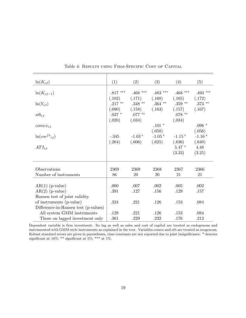
Table 4: Results using Firm-Specific Cost of Capital

ln(Ki,t) (1) (2) (3) (4) (5)

ln(Ki,t−1) .817 ∗∗∗ .468 ∗∗∗ .483 ∗∗∗ .468 ∗∗∗ .493 ∗∗∗

(.102) (.171) (.168) (.165) (.172)ln(Yi,t) .217 ∗∗ .348 ∗∗ .364 ∗∗ .359 ∗∗ .373 ∗∗

(.090) (.158) (.163) (.157) (.167)stbi,t .037 ∗ .077 ∗∗ .078 ∗∗

(.020) (.034) (.034)comexi,t .101 ∗ .098 ∗

(.058) (.056)ln(cocfsi,t) -.345 -1.03 ∗ -1.05 ∗ -1.15 ∗ -1.16 ∗

(.264) (.606) (.625) (.636) (.640)ATIi,t 5.47 ∗ 4.48

(3.33) (3.25)

Observations 2369 2369 2368 2367 2366Number of instruments 86 20 20 21 21

AR(1) (p-value) .000 .007 .002 .005 .002AR(2) (p-value) .391 .127 .156 .129 .157Hansen test of joint validityof instruments (p-value) .324 .221 .126 .153 .084Difference-in-Hansen test (p-values)

All system GMM instruments .129 .221 .126 .153 .084Those on lagged investment only .361 .229 .232 .176 .212

Dependent variable is firm investment. Its lag as well as sales and cost of capital are treated as endogenous andinstrumented with GMM-style instruments as explained in the text. Variables comex and stb are treated as exogenous.Robust standard errors are given in parentheses, time constants are not reported due to joint insignificance. * denotessignificant at 10%; ** significant at 5%; *** at 1%.

19

as compared to expectations.

Estimations (2) and (3) equally point at a cost of capital elasticity close to unity. If the significant

lagged coefficient of the dependent variable is interpreted as being indicative of a partial adjustment

mechanism, the elasticity estimate for the cost of capital only captures the short-term effect. The

long term effect would then be obtained by dividing the cost of capital coefficient by the parameter

estimate of ρ, which is equal to unity minus the coefficient of the lagged dependent variable. With

regard to specifications (2) and (3), the point estimate of the long-run effect is about twice as large

(-1.93 and -2.03) as the basic elasticity estimate. However, due to the large standard errors (1.14

and 1.21), these estimates are not significantly different from (minus) unity. Thus, we cannot reject

the hypothesis that an increase in the cost of capital by one percent implies a decline in the stock

of capital by about 1 percent in the short as well as in the long-run.15

Regarding the magnitude of the tax effect, existing studies report lower elasticities, such as -0.25

(Chirinko, Fazzari and Meyer, 1999) or -0.4 (Chirinko, Fazzari, and Meyer, 2011) or in the range

of -0.5 to -1.0 (Cummins, Hassett and Hubbard, 1994). However, the literature using German data

generally points at slightly larger effects than studies using US data. Harhoff and Ramb (2001)

employ the approach by Chirinko et al. (1999) and yield an elasticity of -0.42 compared to -0.25.

More recently, Dwenger (2010) using an error correction framework reports a point estimate of the

long-term elasticity of about -1.29. A possible explanation for the larger elasticities in the German

context may be the large importance of the local business tax. A high tax burden might exert

stronger empirical effects on investment since firms may respond to a higher tax burden not only

by substituting capital with labor but also in terms of the location of capital.16

Specification in Columns (4) and (5) include another tax variable, the apportionment tax index,

which controls for other effects on the capital stock exerted by the local business tax (for derivation,

see Appendix). As we argued above, due to formula apportionment, it seems likely that the

15To further test for robustness, we attempted to include higher-order lags. While higher-order lags have not been

found to be significant, the specifications suffered from various problems.

16Dwenger and Walsh (2011) use tax loss-carry forwards in order to identify tax incentives and obtain a lowerelasticity for Germany. It is interesting to note, however, that their analysis focuses on the corporation tax. Hence,a likely location incentive of the business tax is not taken into account.

20

statutory tax rate exerts a positive impact on the capital stock due to capital-labor substitution.

While we do find a positive effect, it is only weakly significant. Consistent with the positive

effect, the cost of capital elasticities tend to be slightly larger in columns (4) and (5) – however,

since estimates are not very precise, the differences in the elasticity estimates are not statistically

significant.

6 The Importance of Firm-Specific Differences

Having provided empirical evidence which exploits firm-specific variation in the cost of capital, we

aim at exploring the importance of using this variation for the empirical results. Recall that the

above analysis takes account of firm-specific capital and asset structures as well as of the location-

specific business tax rate. To see whether this is crucial for finding tax effects, in this section, we

abstract from the local variation in tax rates and base the analysis on the assumption that capital

or asset structures are fixed. In a sense, we are employing indicators of a representative rather than

a firm-specific tax burden, something that is often done in the empirical literature analyzing tax

effects.

While Column (2) of Table 5 simply repeats the basic results in the case of firm-specific cost of

capital from above, Columns (6) to (8) provide results where the cost of capital is computed by

making use only of some part of the firm-specific variation. All estimates are obtained from the

two-step system GMM estimator with finite-sample correction and robust standard errors as in

(2). The results displayed in Column (6) report results from a specification where the tax indicator

ignores the firm-specific differences in the capital structure and employs an average figure of the

capital structure. Accordingly, the estimate for the tax effect decreases drastically. Moreover, the

various specification tests indicate problems with this specification since both the Hansen as well as

Difference-in-Hansen tests indicate misspecification. Column (7) reports results of a specification

where the tax indicator takes account of the firm-specific capital structure but employs the average

asset structure. While the estimated coefficient points at a significant effect, the elasticity turns

out to be larger. The results presented in Column (8) have been obtained ignoring the variation

in the local business tax rate. Instead a uniform local business tax rate is used. The results are

21

Table 5: Results using Averages

ln(Ki,t) (2) (6) (7) (8)

ln (Ki,t−1) .468 ∗∗∗ .494 ∗∗∗ .413 ∗∗∗ .471 ∗∗∗

(.171) (.107) (.156) (.166)ln(Yi,t) .348 ∗∗ .328 ∗∗∗ .456 ∗∗∗ .342 ∗∗∗

(.158) (.130) (.155) (.155)stbi,t .077 ∗∗ .075 ∗∗ .053 .079

(.034) (.035) (.037) (.033)ln(cocfsi,t) -1.026∗

(.606)ln(cocavgdebti,t) -.467

(1.79)ln(cocavgassetsi,t) -1.390∗∗

(.708)ln(cocavlocali,t) -1.054

(.639)

Observations 2369 2369 2369 2369Number of instruments 20 20 20 20

AR(1) (p-value) .007 .003 .003 .001AR(2) (p-value) .127 .230 .159 .128Hansen test of joint validityof instruments (p-value) .221 .036 .372 .198Difference-in-Hansen test (p-values)

All system GMM instruments .221 .036 .372 .208Those on lagged investment only .229 .023 .243 .214

Dependent variable is firm investment. Its lag as well as sales and cost of capital are treated as endogenous andinstrumented with GMM-style instruments as explained in the text. Variable stb is treated as exogenous. Robuststandard errors are given in parentheses, time constants are not reported due to joint insignificance. Column (6)report estimation results if an average debt ratio is used for calculating the cost of capital measure, column (7) assumeaverage asset weights, and column (8) reports results where the local tax rate is assumed to be equal to the nationalaverage. * denotes significant at 10%; ** significant at 5%; *** at 1%.

22

not much different from (2), and the point estimate of the effect of the cost-of-capital is almost

not affected. However, probably due to the induced measurement error, the standard error of the

coefficient slightly increases while the Hansen statistic decreases.

7 Summary

While several papers analyzing the relationship between investment and taxation consider homo-

geneous companies, this paper computes firm-and location-specific indicators of the cost of capital

in order to analyze the tax effects on investment decisions. A novel dataset for German firms in

the period 1994 to 2007 is used, which contains balance-sheet as well as survey data and provides

us with information about companies’ financial and asset structures. Additionally, we supplement

information on the local business tax rate faced by each firm.

To analyze the impact of a change in the cost of capital on investment, we estimate a traditional

ADL model as well as a dynamic panel model using GMM techniques which explicitly takes account

of the lag of the capital stock. Along with firm’s sales as an indicator of a firm’s output, we use

the state of business enclosed in the survey data as control variables. The results obtained using

the GMM estimator turn out to be much more convincing than the estimation which relies on the

ADL model.

Our findings indicate a robust, significant negative impact of a firm’s cost of capital on investment,

the elasticity of the cost of capital being in the range of -1 or below. Accordingly, a one percent

increase in the capital cost is associated with a decrease of the capital stock by about 1 percent or

more. As is discussed in the literature, a unit value coefficient should be expected if the elasticity

of substitution between labor and capital is unity. However, our results point at a larger long-

run effect, which could reflect the importance of the local business tax rate for the cost-of-capital.

Arguably, the high local tax burden causes not only substitution effects regarding the capital-labor

ratio but exerts an additional adverse location effect.

To capture some further peculiarities of corporate taxation in Germany, we have also included

23

an indicator that captures incentives arising from formula apportionment for the local business

tax. The results provide some support for the view that, since the formula is based on payroll, –

conditional on the cost of capital – a higher tax burden exerts a separate positive impact on the

capital stock, since firms resort to a higher capital intensity.

We also find that a firm’s appraisal of its current business situation at the time of investment

planning plays an important role in our regressions. Depending on whether the current state of

business is good or bad, investment increases or decreases by almost 8 %. Similarly, optimistic or

pessimistic expectations about the future increase or decrease investment by approximately 10%.

To investigate the role of the local business tax and to analyze the importance of using firm-specific

instead of uniform tax indicators, we consider alternative specifications of the tax incentive by

making specific assumptions about the local business tax rate and about a company’s capital and

asset structures. While tax effects are also found if the firm-specific asset structure is ignored,

abstracting from the firm-specific local business tax rate results in less precise estimates of tax

effects which turn out to be insignificant. A specification ignoring firm-specific differences in the

capital structure does not detect any tax effects and is also plagued with misspecification. Thus,

our results underline the importance of considering firm-specific variation for identifying tax effects,

in particular, the firm-specific variation in the capital structure turns out to be crucial.

Appendix

A.1 Datasource

Firm-level data are taken from the Economics and Business Data Center in Munich which provides

the EBDC dataset combining survey data from the Ifo Business Surveys and financial statement

data from the firm databases Amadeus and Hoppenstedt (see Hoenig, 2010, for an overview).17 By

adding information on tax rates and firm location we can further calculate firm-specific statutory

17Specific information on the Ifo Business Surveys can be found in Becker and Wohlrabe (2008).

24

tax rates and, using balance-sheet information on a firm’s capital and asset structure,18 we can

compute the aforementioned cost of capital variable. This can then be analyzed together with a

firm’s investment, sales and business expectations.

Data from the Ifo Business Survey one has is collected monthly and refers to products instead

of companies. We collapsed the information by year and company after constructing semi-annual

indicators as mentioned in the text.

A.2 German Tax System

During the period 1994-2007 corporations were subject to various income taxes, including the

corporation tax, the business tax on income and capital, and the solidarity surcharge. There are

major changes in the tax law, most important, perhaps, the replacement of the full imputation

and split rate system by the so-called half-income system in 2001. The separate corporation tax

rates - one on retained earnings and one on distributed profits - have been replaced by a lower,

overall tax rate accompanied by a broadening of the tax base. Moreover, the tax credit associated

with dividend payments has been changed from c = 30% to c = 0. As a result, for the time span

1994-2000, γ in equation (2) is equivalent to γ ≡ (1−mD)(1−τdp)(1−c)(1−z)(1−τ) with τdp being the statutory tax

rate on distributed profits including solidarity surcharge and business taxes. Table (A.1) displays

the parameters used in the user cost of capital calculations. Besides the headline rates on retained

earnings (and distributed profits until 2000 in brackets) we present the solidarity surcharge and the

average business tax in our sample for each year. Furthermore, we show the discrimination variable

γ and the statutory tax rates on retained earnings (distributions) including surcharge and business

tax and taking the deductibility of the latter into account.

18We only use balance-sheet information from Hoppenstedt in our estimations.

25

Tab

leA

.1:TaxParametersfortheCost

ofCapital

year

Hea

dli

ne

rate

sre

tain

edea

rnin

gsS

oli

dari

tysu

rcharg

ein

%B

usi

nes

sta

xin

%S

tatu

tory

tax

rate

sre

tain

edea

rnin

gs

γ(d

istr

ibu

ted

pro

fits

)in

%(d

istr

ibu

ted

pro

fits

)in

%

1994

45.0

(30.

0)0

15.9

453.7

6(4

1.1

6)

1.8

219

9545

.0(3

0.0)

7.5

15.9

556.6

1(4

3.0

5)

1.8

719

9645

.0(3

0.0)

7.5

16.1

756.7

2(4

3.2

0)

1.8

719

9745

.0(3

0.0)

7.5

16.3

056.7

9(4

3.2

9)

1.8

719

9845

.0(3

0.0)

5.5

16.4

156.0

9(4

2.8

6)

1.8

619

9940

.0(3

0.0)

5.5

16.4

551.7

1(4

2.8

9)

1.6

920

0040

.0(3

0.0)

5.5

16.1

751.5

4(4

2.7

0)

1.6

920

0125

.05.5

16.4

038.4

51

2002

25.0

5.5

16.2

038.3

01

2003

26.5

5.5

16.0

039.4

91

2004

25.0

5.5

15.9

138.0

91

2005

25.0

5.5

15.9

938.1

51

2006

25.0

5.5

16.0

138.1

61

2007

25.0

5.5

16.1

338.2

51

The

solidari

tysu

rcharg

e’s

ass

essm

ent

base

isth

eov

erall

corp

ora

tein

com

eta

xth

at

has

tob

epaid

.T

her

ew

as

no

solidari

tysu

rcharg

ein

1994.

The

busi

nes

sta

xas

dis

pla

yed

her

eis

calc

ula

ted

as

the

yea

rly

aver

age

out

of

the

sam

ple

,but

we

do

not

acc

ount

for

spec

ific

adju

stm

ents

inth

eco

mputa

tion

of

the

busi

nes

sin

com

e.T

he

basi

cfe

der

al

rate

(Ste

uer

meß

zahl)

is5%

,th

eco

llec

tion

rate

(Heb

esatz

),w

hic

his

fixed

by

munic

ipaliti

es,

isth

eso

urc

eof

vari

ati

on

inth

ebusi

nes

sta

x.

The

statu

tory

tax

rate

sfo

rre

tain

edea

rnin

gs

(dis

trib

ute

dpro

fits

)in

clude

the

solidari

tysu

rcharg

eand

the

busi

nes

sta

xand

are

the

rate

suse

din

our

calc

ula

tions

for

the

firm

-sp

ecifi

cco

stof

capit

al.

26

A.3 Definition of Apportionment Tax Index (ATI)

Since the local business tax is subject to a scheme of formula apportionment, it might tend to further

exert effects on firm decisions. In particular, since payroll serves as formula weight, companies might

use more capital in high-tax jurisdictions. To capture this effect, we construct an apportionment

tax index (ATI) which captures the relative tax burden of a muncipality (in the following, for

simplicity, we suppress the time index t.)

For each firm the business tax TGSt is calculated as TGSt = tGSt(Π− TGSt), where Π is profit and

tGSt = 0.05∗cr100 . cr is the local collection rate in % set by the municipality. Therefore, TGSt can be

written as

TGSt =cr ∗ 0.05

100 + (cr ∗ 0.05)Π =

cr/100 ∗ 0.05

1 + (0.05 ∗ cr/100)Π

With a corporate income tax rate of tKSt (including solidarity surcharge), the corporate income

tax payment TKSt amounts to TKSt = tKSt(Π− TGSt).

Therefore, the total tax burden T is

T = TKSt + TGSt = tKSt(Π− TGSt) + TGSt.

If we consider two jurisdictions and an apportionment of business tax payments according to the

shares s1 and s2, with s1 + s2 = 1, the business tax burden in both jurisdictions results as

TGSti = tGSti (Πsi − TGSti ) =tGSti siΠ

1 + tGSti

, ∀ i = 1, 2,

with TGSt = TGSt1 + TGSt2 and∆TGSti

∆si≥ 0.

As a consequence, the total tax burden amounts to

T = tKSt[Π− tGSt1 s1Π

1 + tGSt1

− tGSt2 s2Π

1 + tGSt2

] +tGSt1 s1Π

1 + tGSt1

+tGSt2 s2Π

1 + tGSt2

.

27

Rearranging this expression we obtain

T = tKStΠ +(1− tKSt)tGSt1 (s1 + s2) Π

1 + tGSt1

+ Πs2

[(1− tKSt)tGSt2

1 + tGSt2

− (1− tKSt)tGSt1

1 + tGSt1

]. (A.13)

Accordingly, the overall tax burden can be described by the federal tax burden and the local tax

burden in municipality 1. In addition, we have some third term that captures the tax burden on the

formula weight. To interpret this term, assume that a company is located in municipality 1, where

the business tax is smaller than in municipality 2, i.e. tGSt2 > tGSt1 . As a consequence, this third

term is positive. Due to the apportionment, the firm obtains a reduction in the total tax burden

if employment in region 2 is reduced such that s2 declines. This last term, therefore, captures the

incentive to distort the formula weight.

To capture this incentive we determine some general reference point and define the apportionment

tax indicator (ATI) for a selected year as follows.

ATIi ≡(1− tKSt)tGSti

1 + tGSti

−(1− tKSt)tGStR

1 + tGStR

.

Obviously, we have ∆ATIi∆tGSti

≥ 0. As reference point we choose the municipality with the minimum

tax rate. Until 2003, we can assume that tGStR = 0, whereas we have tGStR = 0.05∗200100 due to the

minimum collection rate of 200% introduced by the federal legislator in 2004.

References

Arellano, M., and S. Bond (1991). Some Tests of Specification for Panel Data: Monte CarloEvidence and an Application to Employment Equations. The Review of Economic Studies58, 277-297.

Arellano, M., and O. Bover (1995). Another look at the Instrumental Variable Estimation ofError-Component Models. Journal of Econometrics 68, 29-51.

Auerbach, A. J. (1985). The Theory of Excess Burden and Optimal Taxation. In: Auerbach, A.J. and M. Feldstein (ed.), Handbook of Public Economics, chapter 2, 61-127.

Beck, T., Levine, R., and N. Loayza (2000). Finance and the Sources of Growth. Journal ofFinancial Economics 58, 261-300.

Becker, S. O., and K. Wohlrabe (2008). Micro Data at the Ifo Institute for Economic Re-search: The Ifo Business Survey, Usage and Access. Journal of Applied Social Science Studies

28

(Schmollers Jahrbuch), 128(2), 307-319.

Blundell, R., and S. Bond (1998). Initial Conditions and Moment Restrictions in Dynamic PanelData Models. Journal of Econometrics 87, 115-143.

Bond, S., Hoeffler, A., and J. R. Temple (2001). GMM Estimation of Empirical Growth Models.CEPR Discussion Paper No. 3048.

Chirinko, R. S. (1993). Business Fixed Investment Spending: A Critical Survey of ModelingStrategies, Empirical Results, and Policy Implications. Journal of Economic Literature 31,1875-1911.

Chirinko, R. S., Fazzari, S. M., and A. P. Meyer (1999). How responsive is Business CapitalFormation to its User Cost? An Exploration with Micro Data. Journal of Public Economics74, 53-80.

Chirinko, R. S., Fazzari, S. M., and A. P. Meyer (2011). A New Approach to Estimating Pro-duction Function Parameters: The Elusive Capital-Labor Substitution Elasticity. Journal ofBusiness and Economic Statistics forthcoming.

Cummins, J. G., Hassett, K. A., and R. G. Hubbard (1994). A Reconsideration of Investment Be-haviour Using Tax Reforms as Natural Experiments. Brookings Papers on Economic Activity2, 1-74.

DeMooij, R. A., and S. Ederveen (2003). Taxation and Foreign Direct Investment: A Synthesisof Empirical Research. International Tax and Public Finance, 10, 673-693.

Devereux, M. P. (2004). Measuring Taxes on Income From Capital. In: Sørensen, P. B. (ed.),Measuring the Tax Burden on Capital and Labor, MIT Press, Cambridge, chapter 2.

Devereux, M. P., Elschner, C., Endres, D., Heckemeyer, J. H., Overesch, M., Schreiber, U., andC. Spengel (2008). Project for the EU Commission TAXUD/2005/DE/3 10, Final Report.Mannheim, Oxford.

Devereux, M. P., and R. Griffith (1998). Taxes and the Location of Production: Evidence from aPanel of US Multinationals. Journal of Public Economics 68(3), 335-367.

Devereux, M. P., and R. Griffith (1999). The Taxation of Discrete Investment Choices. Institutefor Fiscal Studies, Working Paper 98/16.

Devereux, M. P., and R. Griffith (2003). Evaluating Tax Policy for Location Decisions. Interna-tional Tax and Public Finance 10, 107-126.

Dwenger, N. (2010). User cost elasticity of capital revisited. Mimeo.

Dwenger, N., and F. Walch (2010). Tax Losses and Firm Investment: Evidence from Tax Statistics.Mimeo.

Gordon, R. and J.D. Wilson (1986). An examination of multijurisdictional corporate in- cometaxation under formula apportionment. Econometrica 54, 1357-1373.

Griliches, Z., and J. A. Hausman (1986). Errors in Variables in Panel Data. Journal of Econo-metrics 31, 93-118.

Hall, R. E., and D. W. Jorgenson (1967). Tax Policy and Investment Behaviour. AmericanEconomic Review 57, 391-414.

Harhoff, D., and F. Ramb (2001). Investment and Taxation in Germany - Evidence from Firm-Level Panel Data. In: Deutsche Bundesbank (ed.), Investing Today for the World of Tomor-row - Studies on the Investment Process in Europe, Springer Verlag, Heidelberg, 47-73.

29

Hassett, K. A., and R. G. Hubbard (2002). Tax Policy and Business Investment. Handbook ofPublic Economics 3, 1293-1343.

Hoenig, A. (2010). Linkage of Ifo Survey and Balance-Sheet Data: The EBDC Business Expec-tations Panel & the EBDC Business Investment Panel. Schmollers Jahrbuch 130 (4) 2010,Duncker & Humblot, Berlin.

Jensen, M. C., and W. H. Meckling (1976). Theory of the Firm: Managerial Behavior, AgencyCosts and Ownership Structure. Journal of Financial Economics 3, 305-360.

Jorgenson, D. W. (1963). Capital Theory and Investment Behaviour. American Economic Review53, 247-259.

King, M. A. (1974). Taxation, Investment and the Cost of Capital. Review of Economic Studies41, 21-35.

McDonald, R. L. (2001), Cross-Border Investing with Tax Arbitrage: The Case of German Divi-dend Tax Credits, Review of Financial Studies 14(3), 617-657.

Myers, S. C. (1977). Determinants of Corporate Borrowing. Journal of Financial Economics 3,799-819.

Nickell, S. J. (1981). Biases in Dynamic Models with Fixed Effects. Econometrica 49(6), 1417-1426.

OECD (1991). Taxing Profits in a Global Economy. Paris: OECD.

Roodman, D. (2006). How to do xtabond2: an introduction to ‘Difference’ and ‘System’ GMM inStata. Center for Global Development, Working Paper No. 103.

Roodman, D. (2008). A Note on the Theme of Too Many Instruments. Oxford Bulletin ofEconomics and Statistics, Department of Economics, University of Oxford, 71(1), 135-158.

Sinn, H.-W. (1991). Taxation and the Cost of Capital: The ‘Old’ View, the ‘New’ View andAnother View. In: Bradford, D. (ed.), Tax Policy and the Economy, Vol. 5, Cambridge, MA:MIT Press, 25-54.

Sinn, H.-W. (1987). Capital Income Taxation and Resource Allocation. Amsterdam: North-Holland.

Yoo, K. (2003). Corporate Taxation of Foreign Direct Investment Income 1991-2001. OECDEconomics Department Working Papers No. 365, OECD Publishing.

30

TaxFACTs Schriftenreihe (seit 2006)

Download unter: http://www.steuerinstitut.wiso.uni-erlangen.de/publikationen

Nummer Autor(en) Titel

2006-01 Berthold U. Wigger Do Complex Tax Structues Imply Poorly CraftedPolicies

2006-02 Daniel Durrschmidt Tax Treaties and Most-Favoured-Nation Treat-ment, particularly within the European Union

2006-03 Wolfram SchefflerSusanne Kolbl

Besteuerung der betrieblichen Altersversorgungauf Ebene des Arbeitnehmers im internationalenKontext

2006-04 Michael Glaschke Unabhangigkeit von Bilanzpolitik im IFRS-Einzelabschluss und in der Steuerbilanz

2006-05 Simone Juttner Grenzuberschreitende Verschmelzung uber eineEuropaische Aktiengesellschaft am Beispiel vonDeutschland, Frankreich und Osterreich

2007-01 Berthold U. Wigger Subsidization versus Public Provision of Ter-tiaryEducation in the Presence of Redistributive IncomeTaxation

2007-02 Wolfram Scheffler Grenzuberschreitende Verlustverrechnung nach derRechtsprechung des EuGH in der Rechtssache“Marks&Spencer”

2007-03 Carolin Bock Der Wegzug im Alter aus steuerlicher Sicht: Einelohnende Alternative?

2008-01 Stefanie Alt Steuersystematische Abbildung anteilsbasierterVergutungssysteme im Einheitsunternehmen undim Konzern

2008-02 Wolfram SchefflerEva Okrslar

Die inlandische Auslandsholding als Steuerpla-nungsinstrument nach der Unternehmensteuer-reform 2008

2008-03 Alexander von KotzebueBerthold U. Wigger

Charitable Giving and Fundraising: When Benefi-ciaries Bother Benefactors

32

2008-04 Alexander von KotzebueBerthold U. Wigger

Private Contributions to Collective Concerns:Modeling Donor Behavior

2008-05 Eva Okrslar Besteuerung der identitatswahrenden Verlegungdes Orts der Geschaftsleitung von Kapitalge-sellschaften in einen anderen Mitgliedstaat der Eu-ropaischen Union

2009-01 Christoph Ries Konsolidierte Korperschaftsteuerbemessungsgrundlagein der EU unter Berucksichtigung von Drittstaat-seinkunften

2009-02 Simone Juttner Share Deal versus Asset Deal bei nationalenUbertragungen von Kapitalgesellschaften

2010-01 Wolfram SchefflerHarald Kandel

Sonderausgaben: Versuch einer Systematisierung

2011-01 Carolin Bock Die Vorteilhaftigkeit hybrider Finanzinstrumentegegenuber klassischen Finanzierungsformen –Eine Unternehmenssimulation unter steuerlichenRahmenbedingungen

2011-02 Wolfram Scheffler Innerstaatliche Erfolgszuordnung als Instrumentder Steuerplanung

2011-03 Johannes Riepolt Der Zwischenwert als optimaler Wertansatzbei Verschmelzung von Kapitalgesellschaften –Dargestellt an einem der Zinsschranke unterliegen-den ubertragenden Rechtstrager –

2011-04 Roland Ismer Besteuerung inhabergefuhrter Unternehmens-gruppen: Einschlagige neuere Entwicklungen beider ertragsteuerlichen Organschaft

2011-05 Thiess ButtnerAnja Honig

Investment and Firm-Specific Cost of Capital: Ev-idence from Firm-Level Panel Data

33