investment demand and estructural change
TRANSCRIPT

Economics Working Paper Series
Working Paper No. 1668
Investment demand and estructural change
Manuel García-Santana, Josep Pijoan-Mas, and Lucciano Villacorta
August 2019
Investment Demand and Structural Change∗
Manuel Garcıa-SantanaUPF, Barcelona GSE, CREi and CEPR
Josep Pijoan-MasCEMFI and CEPR
Lucciano VillacortaBanco Central de Chile
August 2019
Abstract
In this paper we study the joint evolution of the investment rate and the sec-toral composition of developing economies. Using panel data for several countriesin different stages of development we document three novel facts: (a) both the in-vestment rate and the industrial weight in the economy are strongly correlated andfollow a hump-shaped profile with development, (b) investment goods contain moredomestic value added from industry and less from services than consumption goodsdo, and (c) the evolution of the sectoral composition of investment and consumptiongoods differs from the one of GDP. We build and estimate a multi-sector growthmodel to fit these patterns. Our results highlight a novel mechanism of structuralchange: the evolution of the investment rate driven by the standard income andsubstitution effect of transitional dynamics explains half of the hump in industrywith development, while the standard income and relative price effects explain therest. We also find that the evolution of investment demand is quantitatively im-portant to understand the industrialization of several countries since 1950 and thedeindustrialization of many Western economies since 1970.
JEL classification: E23; E21; O41Keywords : Structural Change; Investment; Growth; Transitional Dynamics
∗The authors thank valuable comments by Dante Amengual, Rosario Crino, Doug Gollin, BertholdHerrendorf, Joe Kaboski, Tim Kehoe, Rachel Ngai, Marcel Timmer and attendants to seminars held atSTLAR Conference (St. Louis), World Bank, Dartmouth, Cornell, CUNY, Stony Brook, Bank of Spain,CEMFI, Goethe University Frankfurt, Institute for Advanced Studies (Vienna), Universitat Autonomade Barcelona, Universitat de Barcelona, University of Groningen, University of Mannheim, UniversidadeNova de Lisboa, University of Southampton, Universitat de Valencia, Universidade de Vigo, the XXXVIIISimposio of the Spanish Economic Association (Santander), the Fall-2013 Midwest Macro Meeting (Min-nesota), the 2015 meetings of the SED (Warsaw), the MadMac Conference in Growth and Develop-ment (Madrid), and the 2016 CEPR Macroeconomics and Growth Programme Meeting (London). JosepPijoan-Mas acknowledges financial support from Fundacion Ramon Areces and from the Ayuda FundacionBBVA a Investigadores y Creadores Culturales 2016. Postal address: CEMFI, Casado del Alisal 5, 28014Madrid, Spain. E-mail: [email protected], [email protected], [email protected]
1 Introduction
The economic development of nations begins with a rise in industrial production and
a relative decline of agriculture, followed by a decrease of the industrial sector and a
sustained increase of services.1 Because this structural transformation is relatively slow
and associated with long time periods, the recent growth literature has studied changes
in the sectoral composition of growing economies along the balanced growth path, that is
to say, in economies with constant investment rates.2
However, within the last 60 years a significant number of countries have experienced
long periods of growth that may be well characterized by transitional dynamics. For
instance, Song, Storesletten, and Zilibotti (2011) and Buera and Shin (2013) document
large changes in the investment rate of China and the so-called Asian Tigers over several
decades after their development process started. Interestingly, these same countries ex-
perienced a sharp pattern of sectoral reallocation during the period, which suggests that
deviating from the balanced growth path hypothesis might be relevant when thinking
about the causes and consequences of structural transformation.
In this paper we look into the joint determination of the investment rate and the
sectoral composition of developing economies. To do so, we start by documenting three
novel facts. First, using a large panel of countries from the Penn World Tables, we show
that the investment rate follows a long-lasting hump-shaped profile with development,
and that the peak of the hump of investment happens at a similar level of development as
the peak in the hump of industry. Furthermore, this hump-shaped profile of investment is
also present in the long time series data of early developers like Austria, France, Germany
or Netherlands. Second, using Input-Output (IO) tables from the World Input-Output
Database (WIOD), we show that the set of goods used for final investment is different
from the set of goods used for final consumption. Specifically, taking the average over
all countries and years, 55% of the domestic value added used for final investment comes
from the industrial sector, while 42% comes from services. In contrast, only 15% of
1The description of this process traces back to contributions by Kuznets (1966) and Maddison (1991).See Herrendorf, Rogerson, and Valentinyi (2014) and references therein for a detailed description of thefacts.
2Kongsamut, Rebelo, and Xie (2001) study the conditions for structural change due to non-unitaryincome elasticity of demand, while Ngai and Pissarides (2007) model the role of asymmetric productivitygrowth and non-unitary price elasticity. Boppart (2014) shows that both mechanisms can be combinedin balanced growth path with a general type of preferences. In contrast, a third mechanism of structuralchange emphasized in the recent literature —the heterogeneity of production functions across sectors— isincompatible with balanced growth paths although Acemoglu and Guerrieri (2008) and Alvarez-Cuadrado,VanLong, and Poschke (2018) show that quantitatively the aggregate dynamics of these models arequantitatively close to a balanced growth path.
1
domestic value added used for final consumption comes from industry, while 80% come
from services. Therefore, investment goods are 40 percentage points more intensive in
value added from the industrial sector than consumption goods. And third, we document
that there is structural change within both consumption and investment goods, but that
the process is more intense within consumption goods. Furthermore, the standard hump-
shaped profile of industry with development is absent when looking at investment and
consumption goods separately.
Given these facts, we propose a novel mechanism of structural transformation. Be-
cause investment goods incorporate more value added from industry and less from services,
increases in the investment rate increase the demand of industrial value added relative
to services. Conversely, a decrease in the investment rate shifts the composition of the
economy towards services and away from industry. This is an extensive margin of struc-
tural change, as opposed to the intensive margin given by the change of the sectoral
composition of consumption and investment goods due to non-unitary income and price
elasticities as emphasized by the previous literature.3
To understand the joint determination of the investment rate and the sectoral com-
position of the economy, we build a multi-sector neo-classical growth model with three
distinct characteristics. First, we allow for the sectoral composition of the two final goods,
consumption and investment, to be different and endogenously determined through the
standard mechanisms of non-unitary income and price elasiticities. Second, household
preferences over consumption feature a reference level modelled as an external habit.
And third, the sectoral production functions are identical CES with potentially different
Hicks-neutral technology progress. The first of these elements is needed to have an opera-
tive extensive margin of structural change and an endogenous relative price of investment
driving the dynamics of the investment rate. The consumption reference level and the
CES production functions are needed to produce rich transitional dynamics, something
that will be key to match the behaviour of the investment rate.
Our main empirical exercise consists of estimating this model with the big panel of
countries that we use to provide the three main stylized facts described above. We use
the demand system of the model to estimate the parameters characterizing the sectoral
composition of investment and consumption goods, and we estimate the rest of parameters
by asking the model to produce a hump of investment as in the data. Our results are as
follows. First, the model reproduces well the stylized evolution of the investment rate and
3The terms extensive and intensive margin represent a slight abuse of standard terminology: ourextensive margin is not related to a 0-1 decision —countries always invest a positive amount— but tothe change in the relative importance of consumption vs. investment.
2
the sectoral composition of consumption, investment, and GDP. Key elements of this fit
are: a very low elasticity of substitution of sectoral value added within both consumption
and investment; an income elasticity of manufacturing demand within consumption larger
than one in the first half of the development process; sectoral production functions that
feature an elasticity of substitution between capital and labor close to but less than one;
and a strong and persistence reference level in consumption. Second, we find that the
secular increase of productivity in the industrial sector relative to services accounts for
2/3 of the observed fall of the relative price of investment with development. Despite this,
asymmetric sectoral productivity growth has little impact on the path of the investment
rate because the evolution of the relative price of investment has only second order effects
in shaping the investment rate. Our model produces the investment hump mostly as a
result of the interplay of the income and substitution effect of the transitional dynamics
of the model. And third, the extensive margin of structural change explains 1/2 of the
increase and 1/2 of the fall of manufacturing with development. That is, the hump of
investment rate produced by the transitional dynamics of the model generates half of
the hump in manufacturing. The other half is explained by the well-known forces of
non-unitary income and price elasticities combined with income growth and assymmetric
sectoral productivity growth. In particular, during the first half of the development
process the increase in the investment rate and a larger than one income elasticity of
demand of manufactures within consumption raise the overall size of the industrial sector
despite the secular improvement in its technology and the low elasticity of substitution.
The decline of manufacturing in the second half of the development process is explained
by the investment decline and the continued relative improvement in technology within
the industrial sector.
In order to assess the relative importance of the extensive and intensive margins for
particular development episodes, we also perform the estimation of the demand system
separately for 48 different countries between 1950 and 2011 using data from the World
Development Indicators (WDI) and the Groningen 10 Sector Database (G10S). Our results
imply that the changes in investment demand are quantitatively important for structural
change in many countries, especially those in deep transition. Increases in the investment
rate account for a large part of the increase in the size of the industrial sector in South
Korea, Malaysia, and Thailand until the early 90’s, China and India since the early
50’s, Japan and Taiwan until the early 70’s, and Indonesia (1965-2011), Paraguay (1962-
1980) and Vietnam (1987-2007). For this group of countries and years, the share of
the manufacturing sector increased on average by 18.6 percentage points, of which 1/2 is
accounted for by the increase in the investment rate. The investment decline since the 70’s
3
in some rich countries also helps explain the contraction of their manufacturing sectors. In
particular, this was the case in Japan, Finland, Germany, Sweden, Denmark, and Austria
since the early 70’s or Singapore, Philippines and Argentina since the late 70’s or early
80’s. On average, these countries saw a decline in manufactures of 9.5 percentage points,
of which 2/3 came from the decline of the investment rate.
There is a number of papers describing economic mechanisms that could potentially
generate a hump in manufacturing for closed economies. The Ngai and Pissarides (2007)
model with different constant rates of growth in sectoral productivities may lead to humps
in value added shares of those sectors with intermediate rates of productivity growth.
Within the demand-side explanations for structural change, the well-known model with
Stone-Geary preferences of Kongsamut, Rebelo, and Xie (2001) may potentially generate a
hump in transitional dynamics if one moves away from the assumptions that guarantee ex-
istence of a balanced growth path. Other ways of modelling non-homotheticities that can
generate the hump are for instance the hierarchic preferences in Foellmi and Zweimuller
(2008), the scale technologies in Buera and Kaboski (2012b), the non-homothetic CES
preferences in Comin, Lashkari, and Mestieri (2015), or the intertemporally aggregable
preferences in Alder, Boppart, and Muller (2019). All these mechanisms require the hump
of manufacturing to be present within consumption goods. Our story instead allows for
the share of manufacturing value added within final consumption goods to be monotonic,
with the hump in the economy-wide share of manufacturing coming from the hump in
the investment rate. Our empirical evidence finds only weak hump-shaped profiles of the
share of manufacturing value added within consumption. We take this as evidence in favor
of the extensive margin channel. Our results for particular development episodes suggest
that open economy models may also contribute to produce a hump of manufacturing in
GDP that is absent in consumption through an extensive margin of structural change
based on exports instead of investment.4
Finally, a recent paper by Herrendorf, Rogerson, and Valentinyi (2018) measures the
evolution of the sectoral shares within consumption and investment by use of the long time
series of IO data for the US. Their results resemble our findings both in WIOD and WDI-
G10S data. Both their and our paper emphasize the importance of properly accounting for
4There are few models of structural change with open economies that look into the manufacturinghump. For instance, Uy, Yi, and Zhang (2014) argue that sectoral specialization due to productivitygrowth and international trade can generate a hump of manufacturing in GDP, although their quantitativeexercise with Korean data cannot reproduce the falling part of the hump. Matsuyama (2017) model oftrade and non-homothetic demands may also generate a hump of manufacturing in developing economiesthrough sectoral specialization and international trade if the price-elasticity of manufactured goods is inbetween the ones of agriculture and services, although no measurement is provided.
4
the sectoral composition of investment goods when analyzing structural transformation
and its macro consequences. Our paper differs from theirs in one fundamental aspect. We
focus on understanding structural change in contexts where the extensive margin matters,
while they concentrate on the the US, whose dynamics are reasonably close to a balanced
growth path for the 1947-2015 period. In that sense, we model and estimate the joint
determination of the sectoral composition of the economy and the investment rate, while
their paper focuses on estimating the mechanisms operating on the intensive margin only.
In contrast, their focus is on characterizing the balanced growth path properties of their
structural model. In particular, they show that balanced growth path definition imposes
a non-linear restriction on the evolution of sectoral TFP, and find that this restriction
holds for the analyzed period in the US. To our knowledge, they are also the first ones
to use the terms intensive and extensive margins of structural change, which we have
borrowed for this version of our paper.
The remaining of the paper is organized as follows. In Section 2 we show the key
empirical facts that motivate the paper. In Section 3 we outline the model and in Section
4 we discuss its estimation with a large panel of countries. Then, in Section 5 we present
our results for selected development episodes with a country by country estimation of the
demand system of our model. Finally, Section 6 concludes.
2 Some Facts
In this section we present empirical evidence of the three key facts that motivate the paper.
As it is standard in this literature, we divide the economy in three sectors: agriculture,
industry, and services, and use the term manufacturing and industry interchangeably to
denote the second of them, which includes: mining, manufacturing, electricity, gas, and
water supply, and construction.5
2.1 The investment rate and the sectoral composition of the economy
First, we want to characterize the evolution of investment rate with development and its
relationship with the sectoral composition of the economy. To do so, we use investment
data from the Penn World Tables (PWT) and sectoral data from the World Development
Indicators (WDI) and the Groningen 10-Sector Database (G10S) for a large panel of
countries.6 We pool together the data of all countries and years and filter out cross-
5See Appendices A and B for details.6See Section 4.1 for details on the data series and the sample construction. Feenstra, Inklaar, and
Timmer (2015) and Timmer, de Vries, and de Vries (2014) provide a full description of the PWT and
5
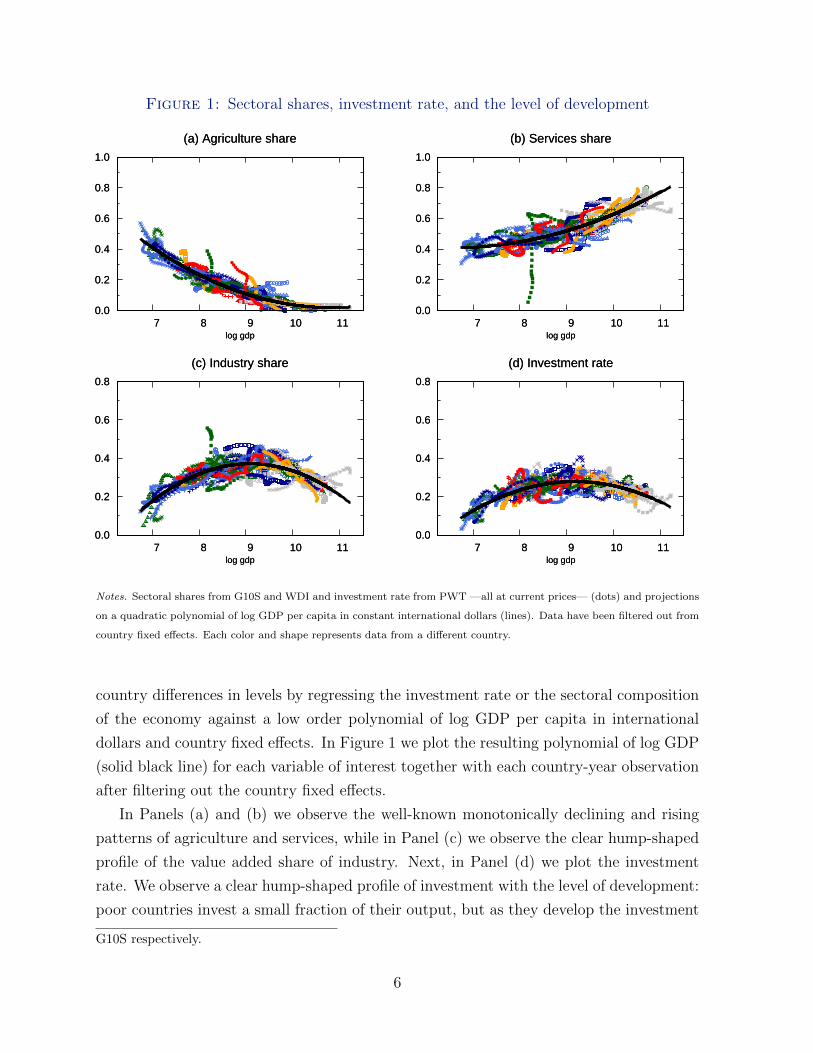
Figure 1: Sectoral shares, investment rate, and the level of development
0.0
0.2
0.4
0.6
0.8
1.0
7 8 9 10 11log gdp
(a) Agriculture share
0.0
0.2
0.4
0.6
0.8
1.0
7 8 9 10 11log gdp
(a) Agriculture share
0.0
0.2
0.4
0.6
0.8
1.0
7 8 9 10 11log gdp
(b) Services share
0.0
0.2
0.4
0.6
0.8
1.0
7 8 9 10 11log gdp
(b) Services share
0.0
0.2
0.4
0.6
0.8
7 8 9 10 11log gdp
(c) Industry share
0.0
0.2
0.4
0.6
0.8
7 8 9 10 11log gdp
(c) Industry share
0.0
0.2
0.4
0.6
0.8
7 8 9 10 11log gdp
(d) Investment rate
0.0
0.2
0.4
0.6
0.8
7 8 9 10 11log gdp
(d) Investment rate
Notes. Sectoral shares from G10S and WDI and investment rate from PWT —all at current prices— (dots) and projections
on a quadratic polynomial of log GDP per capita in constant international dollars (lines). Data have been filtered out from
country fixed effects. Each color and shape represents data from a different country.
country differences in levels by regressing the investment rate or the sectoral composition
of the economy against a low order polynomial of log GDP per capita in international
dollars and country fixed effects. In Figure 1 we plot the resulting polynomial of log GDP
(solid black line) for each variable of interest together with each country-year observation
after filtering out the country fixed effects.
In Panels (a) and (b) we observe the well-known monotonically declining and rising
patterns of agriculture and services, while in Panel (c) we observe the clear hump-shaped
profile of the value added share of industry. Next, in Panel (d) we plot the investment
rate. We observe a clear hump-shaped profile of investment with the level of development:
poor countries invest a small fraction of their output, but as they develop the investment
G10S respectively.
6

rate increases up to a peak and then it starts declining. Note that the hump is long-lived
(it happens while GDP multiplies by a factor of 100), it is large (the investment rate
increases by 20 percentage points), and it is present for a wide sample of countries (48
countries at very different stages of development). A hump of investment with the level
of development has already been documented with relatively short country time series for
the Asian Tigers, (see Buera and Shin (2013)), and Japan and OCDE countries after the
IIWW (see Christiano (1989), Chen, Imrohoroglu, and Imrohoroglu (2007) and Antras
(2001)). Here we show this pattern to be very systematic. Indeed, we show in Appendix C
that with the long time series assembled by Jorda, Schularick, and Taylor (2017), a hump
of investment with development is also prevalent among early starters. Furthermore,
we can see that the hump in industrial production in Panel (c) is very similar in size
to the hump in investment in Panel (d), with the peak happening at a similar level of
development. Indeed, the correlation between the value added share of industry and the
investment rate is 0.44 in the raw data pooling all countries and years, and 0.55 when
controlling for country fixed effects.
2.2 Sectoral composition of investment and consumption goods
The second piece of evidence that we put together is the different sectoral composition
of the goods used for final investment and final consumption. We use the World Input
Output Database (WIOD), which provides IO tables for 35 sectors, 40 countries (mostly
developed), and 17 years (between 1995 and 2011).7 To give an example of what we
do, consider how final investment goods may end up containing value added from the
agriculture sector. Agriculture goods are sold as final consumption to households and
as exports, but not used directly for gross capital formation. However, most of the
output from the agriculture sector is sold as intermediate goods to several industries (e.g.,
“Textiles”) that are themselves sold to other industries (e.g., “Transport Equipment”)
whose output goes to final investment. In short, agricultural value added is indirectly
an input into investment goods. In Appendix B we explain how to obtain the sectoral
composition of each final good following the procedure explained by Herrendorf, Rogerson,
and Valentinyi (2013).
We find that investment goods are more intensive in industrial value added than
consumption goods are, see Table 1. In particular, taking the average over all countries
and years, the value added share of industry is 55% for investment goods (column 2)
7A detailed explanation of the WIOD can be found in Timmer, Dietzenbacher, Los, Stehrer, and deVries (2015).
7
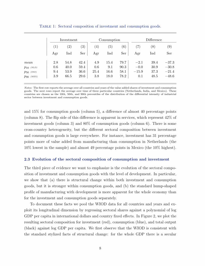
Table 1: Sectoral composition of investment and consumption goods.
Investment Consumption Difference
(1) (2) (3) (4) (5) (6) (7) (8) (9)
Agr Ind Ser Agr Ind Ser Agr Ind Ser
mean 2.8 54.8 42.4 4.9 15.4 79.7 −2.1 39.4 −37.3p10 (NLD) 0.6 40.0 59.4 0.6 9.1 90.3 −0.0 30.9 −30.8p50 (IND) 9.4 53.9 36.6 25.4 16.6 58.1 −15.9 37.3 −21.4p90 (MEX) 3.9 66.5 29.6 3.8 18.0 78.2 0.1 48.5 −48.6
Notes: The first row reports the average over all countries and years of the value added shares of investment and consumptiongoods. The next rows report the average over time of three particular countries (Netherlands, India, and Mexico). Thesecountries are chosen as the 10th, 50th, and 90th percentiles of the distribution of the differential intensity of industrialsector between investment and consumption goods.
and 15% for consumption goods (column 5), a difference of almost 40 percentage points
(column 8). The flip side of this difference is apparent in services, which represent 42% of
investment goods (column 3) and 80% of consumption goods (column 6). There is some
cross-country heterogeneity, but the different sectoral composition between investment
and consumption goods is large everywhere. For instance, investment has 31 percentage
points more of value added from manufacturing than consumption in Netherlands (the
10% lowest in the sample) and almost 49 percentage points in Mexico (the 10% highest).
2.3 Evolution of the sectoral composition of consumption and investment
The third piece of evidence we want to emphasize is the evolution of the sectoral compo-
sition of investment and consumption goods with the level of development. In particular,
we show that (a) there is structural change within both investment and consumption
goods, but it is stronger within consumption goods, and (b) the standard hump-shaped
profile of manufacturing with development is more apparent for the whole economy than
for the investment and consumption goods separately.
To document these facts we pool the WIOD data for all countries and years and ex-
ploit its longitudinal dimension by regressing sectoral shares against a polynomial of log
GDP per capita in international dollars and country fixed effects. In Figure 2, we plot the
resulting sectoral composition for investment (red), consumption (blue), and total output
(black) against log GDP per capita. We first observe that the WIOD is consistent with
the standard stylized facts of structural change: for the whole GDP there is a secular
8
decline of agriculture, a secular increase in services, and a (mild) hump of manufacturing.
When looking at the pattern of sectoral reallocation within each good, we observe that
the share of agriculture declines faster in consumption than in investment, that the share
of services increases faster in consumption than in investment, and that the share of man-
ufacturing declines somewhat faster in consumption than in investment. These patterns
imply that structural change is sharper within consumption than within investment and
that the asymmetry between consumption and investment goods in terms of their content
of manufacturing and services widens with development. Finally, it is important to note
that the hump of manufacturing within GDP is happening neither within investment (the
quadratic term is non-significant) nor within consumption (the increasing part is missing).
The comparison of the share of manufacturing within investment and consumption with
the share of manufacturing for the whole GDP is more clear in Panel (a) of Figure B.1,
which puts together the pics in Panel (e) and (f) of Figure 2.
2.4 A novel mechanism for structural change
The facts described above highlight the potential importance of the composition of final
expenditure for structural change, and suggest a possible explanation for the hump in man-
ufacturing. Standard forces of structural change like non-homotheticities and asymmetric
productivity growth may explain sectoral reallocation within investment and within con-
sumption goods. But because investment goods are more intensive in value added from
manufacturing than consumption goods, the hump-shaped profile of the investment rate
generates a further force of structural change. Consistent with this mechanism, the hump
of manufacturing is more apparent for the whole economy than for the consumption and
investment goods separately.
While the WIOD data may not be ideal to study structural change because of the
short time dimensions and the small number of developing countries, we can still use it to
have a first assessment of our mechanism. To do so we start by using National Accounts
identities to note that the value added share of sector i within GDP can be written as,
VAi
GDP=
(VAx
GDP
)(VAx
i
VAx
)+
(VAc
GDP
)(VAc
i
VAc
)+
(VAe
GDP
)(VAe
i
VAe
)(1)
which is a weighted sum of the sectoral share within investment VAxi /VAx, within con-
sumption VAci/VAc, and within exports VAe
i/VAe. The first two are the objects that we
have documented in Table 1 and in Panel (a), (c), and (e) of Figure 2. The weights
are the domestic investment rate VAx/GDP, domestic consumption rate VAc/GDP, and
9
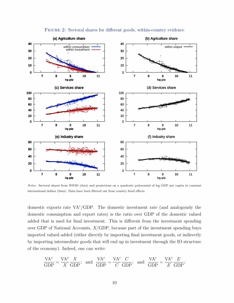
Figure 2: Sectoral shares for different goods, within-country evidence
0
10
20
30
40
7 8 9 10 11log gdp
(a) Agriculture share
within consumptionwithin investment
0
10
20
30
40
7 8 9 10 11log gdp
(a) Agriculture share
0
10
20
30
40
7 8 9 10 11log gdp
(a) Agriculture share
0
10
20
30
40
7 8 9 10 11log gdp
(a) Agriculture share
0
10
20
30
40
7 8 9 10 11log gdp
(a) Agriculture share
0
10
20
30
40
7 8 9 10 11log gdp
(b) Agriculture share
within output
0
10
20
30
40
7 8 9 10 11log gdp
(b) Agriculture share
0
10
20
30
40
7 8 9 10 11log gdp
(b) Agriculture share
0
20
40
60
80
100
7 8 9 10 11log gdp
(c) Services share
0
20
40
60
80
100
7 8 9 10 11log gdp
(c) Services share
0
20
40
60
80
100
7 8 9 10 11log gdp
(c) Services share
0
20
40
60
80
100
7 8 9 10 11log gdp
(c) Services share
0
20
40
60
80
100
7 8 9 10 11log gdp
(d) Services share
0
20
40
60
80
100
7 8 9 10 11log gdp
(d) Services share
0
20
40
60
80
7 8 9 10 11log gdp
(e) Industry share
0
20
40
60
80
7 8 9 10 11log gdp
(e) Industry share
0
20
40
60
80
7 8 9 10 11log gdp
(e) Industry share
0
20
40
60
80
7 8 9 10 11log gdp
(e) Industry share
0
20
40
60
80
7 8 9 10 11log gdp
(e) Industry share
0
20
40
60
80
7 8 9 10 11log gdp
(f) Industry share
0
20
40
60
80
7 8 9 10 11log gdp
(f) Industry share
Notes. Sectoral shares from WIOD (dots) and projections on a quadratic polynomial of log GDP per capita in constant
international dollars (lines). Data have been filtered out from country fixed effects.
domestic exports rate VAe/GDP. The domestic investment rate (and analogously the
domestic consumption and export rates) is the ratio over GDP of the domestic valued
added that is used for final investment. This is different from the investment spending
over GDP of National Accounts, X/GDP, because part of the investment spending buys
imported valued added (either directly by importing final investment goods, or indirectly
by importing intermediate goods that will end up in investment through the IO structure
of the economy). Indeed, one can write:
VAx
GDP=
VAx
X
X
GDP; and
VAc
GDP=
VAc
C
C
GDP; and
VAe
GDP=
VAe
E
E
GDP;
10
where X, C, and E are the expenditure in investment, consumption, and exports. While
by construction the domestic investment rate will be weakly smaller than the actual
investment rate, the evolution of both magnitudes presents a similar hump with the level
of development, see Panel (b) of Figure B.1. Hence, structural change can happen because
there is a change in the sectoral composition of investment, consumption or export goods
(the intensive margin) or because there is a change in the investment, consumption or
export demand of the economy (the extensive margin).
To decompose the evolution of sectoral shares into the intensive and extensive margins,
we do two complementary exercises. In both exercises we build two counterfactual series
for each sectoral share of the economy, in which only the intensive or extensive margin
are active. In the first exercise, which we call “open economy”, the intensive margin
counterfactual holds the VAj/GDP (j = {x, c, e}) terms of the right hand side of equa-
tion (1) equal to their country averages, while the extensive margin counterfactual holds
constant the VAji/VAj (j = {x, c, e}) terms. In the second exercise, which we call “closed
economy”, we first build counterfactual sectoral shares omitting exports and imports as
follows,
VAi
GDP=
X
X + C
(VAx
i
VAx
)+
C
X + C
(VAc
i
VAc
)(2)
Then, we build the intensive margin counterfactual by holding the XX+C
and CX+C
terms
in equation (2) equal to their average and the extensive margin counterfactual by holding
constant the VAji/VAj (j = {x, c}) terms.
We report in Table 2 the average importance of the intensive and extensive margin
of structural change across the 40 countries and 17 years. In the first column, we report
the average change in the share of Agriculture (decline of 26 percentage points), Industry
(decline of 6.1 percentage points, which comes from an initial increase of 4.9 followed by a
decline of 10.9 percentage points), and Services (increase of 32.3 percentage points) across
all countries and years as described in Figure 2. In the third and fourth columns, we report
the change accounted for by the intensive and extensive margins in the “open economy”
exercise.8 We find that the extensive margin is important for the evolution of the industrial
and service sectors. For instance, sectoral reallocation within consumption, investment,
and exports would have implied a decline of industry value added of 16 percentage points,
a fall almost 10 percentage points larger than what we observe. Instead, the variation in
investment, consumption, and export rates pulled the demand for industrial value added
8These changes comes from treating the counterfactual series as the actual data: we pool all yearsand countries together and keep the relationship between sectoral share and log GDP after filtering outcountry fixed effects.
11
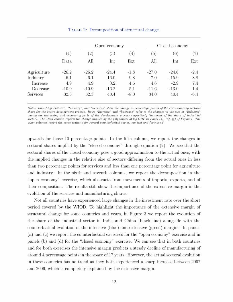
Table 2: Decomposition of structural change.
Open economy Closed economy
(1) (2) (3) (4) (5) (6) (7)
Data All Int Ext All Int Ext
Agriculture -26.2 -26.2 -24.4 -1.8 -27.0 -24.6 -2.4Industry -6.1 -6.1 -16.0 9.8 -7.0 -15.9 8.8
Increase 4.9 4.9 0.2 4.6 4.6 -2.9 7.4Decrease -10.9 -10.9 -16.2 5.1 -11.6 -13.0 1.4
Services 32.3 32.3 40.4 -8.0 34.0 40.4 -6.4
Notes: rows “Agriculture”, “Industry”, and “Services” show the change in percentage points of the corresponding sectoralshare for the entire development process. Rows “Increase” and “Decrease” refer to the changes in the size of “Industry”during the increasing and decreasing parts of the development process respectively (in terms of the share of industrialsector). The Data column reports the change implied by the polynomial of log GDP in Panel (b), (d), (f) of Figure 1. Theother columns report the same statistic for several counterfactual series, see text and footnote 8.
upwards for those 10 percentage points. In the fifth column, we report the changes in
sectoral shares implied by the “closed economy” through equation (2). We see that the
sectoral shares of the closed economy pose a good approximation to the actual ones, with
the implied changes in the relative size of sectors differing from the actual ones in less
than two percentage points for services and less than one percentage point for agriculture
and industry. In the sixth and seventh columns, we report the decomposition in the
“open economy” exercise, which abstracts from movements of imports, exports, and of
their composition. The results still show the importance of the extensive margin in the
evolution of the services and manufacturing shares.
Not all countries have experienced large changes in the investment rate over the short
period covered by the WIOD. To highlight the importance of the extensive margin of
structural change for some countries and years, in Figure 3 we report the evolution of
the share of the industrial sector in India and China (black line) alongside with the
counterfactual evolution of the intensive (blue) and extensive (green) margins. In panels
(a) and (c) we report the counterfactual exercises for the “open economy” exercise and in
panels (b) and (d) for the “closed economy” exercise. We can see that in both countries
and for both exercises the intensive margin predicts a steady decline of manufacturing of
around 4 percentage points in the space of 17 years. However, the actual sectoral evolution
in these countries has no trend as they both experienced a sharp increase between 2002
and 2006, which is completely explained by the extensive margin.
12
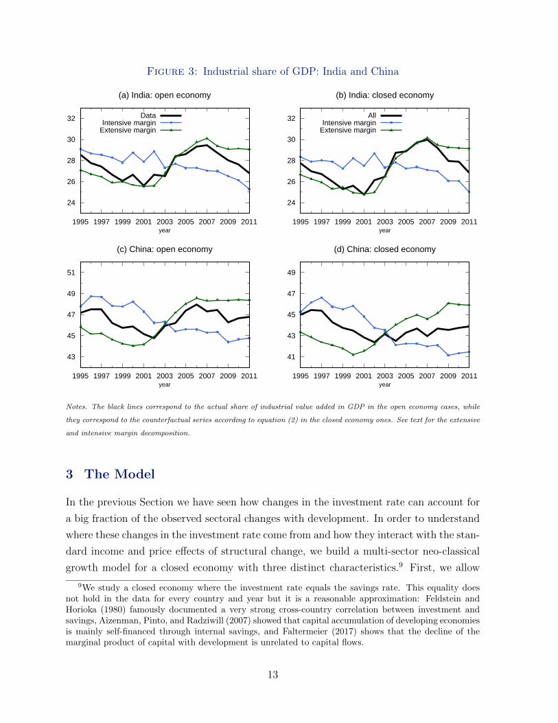
Figure 3: Industrial share of GDP: India and China
24
26
28
30
32
1995 1997 1999 2001 2003 2005 2007 2009 2011year
(a) India: open economy
DataIntensive margin
Extensive margin
24
26
28
30
32
1995 1997 1999 2001 2003 2005 2007 2009 2011year
(b) India: closed economy
AllIntensive margin
Extensive margin
43
45
47
49
51
1995 1997 1999 2001 2003 2005 2007 2009 2011year
(c) China: open economy
41
43
45
47
49
1995 1997 1999 2001 2003 2005 2007 2009 2011year
(d) China: closed economy
Notes. The black lines correspond to the actual share of industrial value added in GDP in the open economy cases, while
they correspond to the counterfactual series according to equation (2) in the closed economy ones. See text for the extensive
and intensive margin decomposition.
3 The Model
In the previous Section we have seen how changes in the investment rate can account for
a big fraction of the observed sectoral changes with development. In order to understand
where these changes in the investment rate come from and how they interact with the stan-
dard income and price effects of structural change, we build a multi-sector neo-classical
growth model for a closed economy with three distinct characteristics.9 First, we allow
9We study a closed economy where the investment rate equals the savings rate. This equality doesnot hold in the data for every country and year but it is a reasonable approximation: Feldstein andHorioka (1980) famously documented a very strong cross-country correlation between investment andsavings, Aizenman, Pinto, and Radziwill (2007) showed that capital accumulation of developing economiesis mainly self-financed through internal savings, and Faltermeier (2017) shows that the decline of themarginal product of capital with development is unrelated to capital flows.
13
for the sectoral composition of the two final goods, consumption and investment, to be
different and endogenously determined. Second, household preferences over consumption
feature a reference level modelled as an external habit. And third, the sectoral production
functions are identical CES with potentially different Hicks-neutral technology progress.
The first of these elements is needed to have an operative extensive margin of struc-
tural change and an endogenous relative price of investment driving the dynamics of the
investment rate. The external habit and the CES production functions are needed to pro-
duce rich transitional dynamics, something that will be key to match the behaviour of the
investment rate. The standard one sector neo-classical growth model with Cobb-Douglas
production and time-separable CRRA utility function features either a monotonically in-
creasing or a monotonically decreasing saving rate along the development path, see Barro
and Sala-i-Martin (1999). A consumption reference level helps produce hump-shaped pro-
files of the saving rate with development because it makes the income effect very strong
at the start of the development process and very weak at the end, see Christiano (1989),
King and Rebelo (1993), and Antras (2001). Modelling the consumption reference level
as an external habit gives both an economic interpretation of this mechanism and a flex-
ible framework for quantitative work.10 An elasticity of substitution between capital and
labor less than one also helps produce investment profiles that are hump-shaped with
development —because the substitution effects is much weaker than with Cobb-Douglas
at low levels of capital (see Antras (2001) and Smetters (2003))— and it helps slow down
the transitional dynamics of the model.
3.1 Set up
The economy consists of three different sectors that produce intermediate goods: agri-
culture, manufacturing, and services, indexed by i = {a,m, s}. Output yit of each sector
can be used both for final consumption cit and for final investment xit. An infinitely-lived
representative households rents capital kt and labor (normalized to one) to firms, and
chooses how much of each good to buy for consumption and investment purposes while
satisfying the standard budget constraint:
wt + rtkt =∑
i={a,m,s}
pit (cit + xit) (3)
10See Carroll, Overland, and Weil (2000) and Alvarez Cuadrado, Monteiro, and Turnovsky (2004) fordifferent versions of habit-based explanations of non-monotonic investment trajectories in the transitionaldynamics of the one-sector neo-classical growth model.
14
where pit is the price of output of sector i at time t, wt is the wage rate, and rt is the
rental rate of capital. Capital accumulates with the standard law of motion
kt+1 = (1− δk) kt + xt (4)
where 0 < δk < 1 is a constant depreciation rate, and xt ≡ Xt(xat, xmt, xst) is the amount
of efficiency units of the investment good produced with a bundle of goods from each sec-
tor. The period utility function is defined over a consumption basket ct ≡ C(cat, cmt, cst)
that aggregates goods from the three sectors. We specify a standard CES aggregator for
investment, whereas we also allow for non-homotheticities in consumption:
C(ca, cm, cs) =
∑i∈{a,m,s}
(θci )1−ρc (ci + ci)
ρc
1ρc
(5)
Xt(xa, xm, xs) = χt
∑i∈{a,m,s}
(θxi )1−ρx xρxi
1ρx
(6)
with ρj < 1, 0 < θji < 1 and∑
i∈{a,m,s} θji = 1 for j ∈ {c, x}, i ∈ {a,m, s}. These two
aggregators differ in several dimensions. First, we allow the sectoral share parameters in
consumption θci to differ from the sectoral share parameters in investment θxi . Second,
we allow the elasticity of substitution, given by 1/(1− ρj), to differ across goods. Third,
we introduce the terms ci in order to allow for non-homothetic demands for consump-
tion. Much of the literature has argued that these non-homotheticities are important to
fit the evolution of the sectoral shares of GDP, and non-unitary income elasticities have
been estimated in the micro data of household consumption. We omit similar terms in
the investment aggregator partly due to the difficulty to separately identify them from ci
in the data and partly due to the lack of micro-evidence.11 Finally, χt captures exoge-
nous investment-specific technical change, a feature that is shown to be quantitatively
important in the growth literature, see Greenwood, Hercowitz, and Krusell (1997) or
Karabarbounis and Neiman (2014). Note that the literature of structural change has typ-
11Agricultural goods are typically modelled as a necessity (ca < 0) because of the strong decline inthe share of agriculture with development. Emphasizing this non-homotheticitiy within consumptiongoods is also consistent with the micro data evidence showing that the budget share for food decreases ashousehold income increases. See for instance Deaton and Muellbauer (1980), Banks, Blundell, and Lewbel(1997), or Almas (2012). Services instead are typically modelled as luxury goods (cs > 0) because theirshare increases with development. A typical interpretation is that services have easy home substitutesand households only buy them in the market after some level of income. See for instance Rogerson (2008)and Buera and Kaboski (2012a).
15
ically assumed that either the aggregators for consumption and investment are the same,
that the investment goods are only produced with manufacturing value added, or that
the investment good is a fourth type of good produced in a fourth different sector.12
3.2 Household problem
Households have a CRRA utility function over the consumption basket ct above a minimal
standard of living φht,
u (ct − φht) =(ct − φht)1−σ
1− σ(7)
where we define ht as follows:
ht = (1− δh)ht−1 + δhct−1 (8)
We think of ht as an external habit. Households value consumption flow ct in relation to
the standard of living ht that they are used to, but they do not internalize the changes in
ht+1 when choosing their own consumption flow ct. The parameter 1 > φ ≥ 0 drives the
strength of the external habit and the parameter 1 ≥ δh ≥ 0 its persistence.
The optimal household plan is the sequence of consumption and investment choices
that maximizes the discounted infinite sum of utilities. We can write the Lagrangian as,
∞∑t=0
βt
u (ct − φht) + λt
[wt + rtkt −
∑i={a,m,s}
pit (cit + xit)]
+ ηt
[(1− δk) kt + xt − kt+1
]where λt and ηt are the shadow values at time t of the budget constraint and the law of
motion of capital respectively. Taking prices as given, the standard first order conditions
with respect to goods cit and xit are:
∂ut (ct)
∂ct
∂ct∂cit
= λt pit i ∈ {a,m, s} (9)
ηt∂xt∂xit
= λt pit i ∈ {a,m, s} (10)
12An example of the first case is Acemoglu and Guerrieri (2008), examples of the second case areEchevarrıa (1997), Kongsamut, Rebelo, and Xie (2001) or Ngai and Pissarides (2007), while examples ofthe third case are Boppart (2014) or Comin, Lashkari, and Mestieri (2015). Instead, Garcıa-Santana andPijoan-Mas (2014) already allow for a different composition of investment and consumption goods andmeasure them in a calibration exercise with Indian data.
16

while the FOC for capital kt+1 is given by,
ηt = β λt+1rt+1 + β ηt+1 (1− δk) (11)
3.3 Consumption composition
Using the utility function in equation (7) and the consumption aggregator in equation
(5), the FOC of each good i described by equation (9) can be rewritten as:
(ct − φht)−σ(θci
ctcit + ci
)1−ρc= λtpit (12)
We can aggregate them (raising to the power ρcρc−1
and summing them up) to obtain the
FOC for the consumption basket,
(ct − φht)−σ = λtpct (13)
where pct is the implicit price index of the consumption basket defined as:
pct ≡
[ ∑i=a,m,s
θci pρcρc−1
it
] ρc−1ρc
(14)
Adding up the FOC for each good i we obtain,∑i=a,m,s
pitcit = pctct −∑
i=a,m,s
pitci (15)
which states that total expenditure in consumption goods is equal to the value of the
consumption basket minus the value of the non-homotheticities. Finally, using equations
(12) and (15) we obtain the consumption expenditure share of each good i:
pitcit∑j=a,m,s pjtcjt
= θci
(pctpit
) ρc1−ρc
[1 +
∑j=a,m,s pjtcj∑j=a,m,s pjtcjt
]− pitci∑
j=a,m,s pjtcjt(16)
3.4 Investment composition
Using the aggregator in equation (6), the FOC of each good i described by equation (10)
can be rewritten as:
ηtχρt
(θxixtxit
)1−ρx= λtpit (17)
17
Following similar steps as for consumption we get the FOC for total investment,
ηt = λtpxt (18)
where
pxt ≡1
χt
[ ∑i=a,m,s
θxi pρxρx−1
it
] ρx−1ρx
(19)
and the total expenditure equation,
pxtxt =∑
i=a,m,s
pitxit (20)
Finally, the actual composition of investment expenditure is obtained combining equations
(17) and (20),
pitxitpxtxt
= θxi
(χt pxtpit
) ρx1−ρx
(21)
3.5 Euler equation
Plugging equations (13) and (18) into (11) we get the Euler equation,
(ct − φht)−σ = β (ct+1 − φht+1)−σpxt+1
pct+1
pctpxt
[rt+1
pxt+1
+ (1− δk)]
(22)
which states that the value of one unit of consumption today must equal the value of
transforming that unit into capital, renting the capital to firms, and consuming the pro-
ceeds next period. The term in square brackets in the right-hand-side is the investment
return in units of the investment good. When divided by the increase in the relative price
of consumption it becomes the investment return in units of the consumption good, which
is the relevant one for the Euler equation.
3.6 Production
There is a representative firm in each sector i = {a,m, s} that combines capital kit and
labor lit to produce the amount yit of the good i. The production functions are CES with
identical share 0 < α < 1 and elasticity ε < 1 parameters. There is a labour-augmenting
common technology level Bt and a sector-specific Hicks-neutral technology level Bit:
yit = Bit
[αkεit + (1− α) (Btlit)
ε ]1/ε18
Assuming CES production functions with Hicks-neutral sector-specific technical progress
extends the canonical Cobb-Douglas multi-sector growth model by allowing for non-
unitary elasticity of substitution between capital and labour while retaining the analytical
tractability of equal capital to labor ratio across sectors.13 The objective function of each
firm is given by,
maxkit,lit{pityit − rtkit − wtlit}
Leading to the standard FOC,
rt = pit α Bεit
(yitkit
)1−ε
(23)
wt = pit (1− α)Bεt B
εit
(yitlit
)1−ε
(24)
3.7 Equilibrium
An equilibrium for this economy is a sequence of exogenous productivity paths {Bt, χt, Bit}∞t=1
where i ∈ {a,m, s}; a sequence of aggregate allocations {ct, xt, yt, kt}∞t=1; a sequence of sec-
toral allocations {kit, lit, yit, xit, cit}∞t=1 ; and a sequence of equilibrium prices {rt, wt, pit, pct, pxt}∞t=1
such that
• Households optimize: equations (9), (10) and (11) hold
• Firms optimize: equations (23), (24) hold
• All markets clear:∑
i=a,m,s kit = kt,∑
i=a,m,s lit = 1, yit = cit + xit for all i = a,m, s
We define GDP yt from the production side as as yt ≡∑
i=a,m,s pityit. Note that the
market clearing conditions and equations (15) and (20) imply that the GDP from the
expenditure side is given by yt = pxtxt +∑
i=a,m,s pitcit = pxtxt + pctct −∑
i=a,m,s pitci
In order to determine the equilibrium prices, note that the FOC of the firms imply
that the capital to labor ratio is the same across all sectors and equal to the capital to
labor ratio in the economy kitlit
= kt, with
kt =
(α
1− αwtrtB−εt
) 11−ε
(25)
13With CES production functions and Hicks-neutral technical progress there is no Balanced GrowthPath, see Uzawa (1961). For this reason, we will later assume that the only source of growth in the longrun is the common labour-augmenting technical progress.
19
Hence, the relative sectoral prices are given by relative sectoral productivities:
pitpjt
=Bjt
Bit
(26)
Finally, we define average productivity in consumption Bct and in investment Bxt as
follows,
Bct ≡
[ ∑i=a,m,s
θciBρc
1−ρcit
] 1−ρcρc
(27)
Bxt ≡
[ ∑i=a,m,s
θxi Bρx
1−ρxit
] 1−ρxρx
(28)
These productivity levels are useful because they summarize all the information on sectoral
productivities that is needed to describe the aggregate dynamics of the homothetic version
of our economy (ci = 0), and also the aggregate dynamics around the asymptotic Balanced
Growth Path. In fact, Bct and χtBxt can be thought of as the Hicks-neutral productivity
levels in a two good economy that produces consumption and investment goods with
otherwise identical CES production functions in capital and labor.14 Using the definitions
of pct and pxt in equations (14) and (19) we can write,
pitpct
=Bct
Bit
andpitpxt
= χtBxt
Bit
(29)
and alsopxtpct
=1
χt
Bct
Bxt
(30)
Hence, the relative price of investment has two components: the exogenous investment-
specific technical change χt and the endogenous evolution of the relative productivity
of investment and consumption Bxt/Bct driven by the changes in the relative sectoral
productivities. Note also that equations (26), (29), and (30) determine relative prices but
that the overall price of the economy (and its revolution) is undetermined. We will use
the investment good as numeraire when we study the aggregate dynamics of the economy
with hat variables. For that purpose, it will be useful to write the expressions for output
14See Appendix D.4 for details.
20
and the interest rate in units of the investment good as follows:
yt/pxt = χtBxt
[αkεt + (1− α)Bε
t
]1/ε(31)
rt/pxt = α (χtBxt)ε
(yt/pxtkt
)1−ε
= αχtBxt
[α + (1− α)
(Bt
kt
)ε] 1−εε
(32)
3.8 Sectoral shares
Using the market clearing conditions for each good i ∈ {a,m, s}, we can express the
sectoral shares of GDP at current prices with the following identities:
pityityt
=pitxitpxtxt
pxtxtyt
+pitcit∑
j=a,m,s pjtcjt
(1− pxtxt
yt
)i ∈ {a,m, s} (33)
This states that the value added share of sector i in GDP is given by the share of sector i
within investment times the investment rate plus the share of sector i within consumption
times the consumption rate. The sectoral shares within consumption and investment are
obtained from the demand system of the static problem, see equations (16) and (21).
Using the expressions for pct and pxt in equations (14) and (19) we can obtain,
pitcit∑j=a,m,s pjtcjt
=
[ ∑j=a,m,s
θcjθci
(pitpjt
) ρc1−ρc
]−1 [1 +
∑j=a,m,s pjtcj∑j=a,m,s pjtcjt
]− pitci∑
j=a,m,s pjtcjt(34)
pitxitpxtxt
=
[ ∑j=a,m,s
θxjθxi
(pitpjt
) ρx1−ρx
]−1
(35)
Therefore, structural change will happen because of sectoral reallocation within consump-
tion due to both income and price effects, because of sectoral reallocation within invest-
ment due to price effects only, and because of reallocation in expenditure between con-
sumption and investment in transitional dynamics, i.e., changes in the investment rate.
The first two form the intensive margin of structural change, while the third one is the
extensive margin of structural change. The larger the difference in sectoral composition
between investment and consumption goods, the stronger this latter effect.
3.9 Aggregate dynamics
We have three difference equations to characterize the aggregate dynamics of this economy:
the Euler equation of consumption in equation (22), the law of motion of capital in
equation (4), and the law of motion for the habit stock given by equation (8). After
21
substituting prices away the first two become,
[ct+1 − φht+1
ct − φht
]σ= β
[Bct+1
Bct
Bxt
Bxt+1
χxtχxt+1
] [αχt+1Bxt+1
[α + (1− α)
(Bt+1
kt+1
)ε] 1−εε
+ (1− δk)
](36)
and
kt+1
kt= (1− δk) + χtBxt
[α + (1− α)
(Bt
kt
)ε]1/ε
− χtBxt
Bct
ctkt
(1−
∑i=a,m,s
BctciBitct
)(37)
The dynamic system is driven by the three primitive sources of technological change:
the economy-wide labor saving technology Bt, the sector-specific Hicks neutral technol-
ogy Bit (which enter directly, but also indirectly through the endogenous investment and
consumption specific Hicks neutral technology levels Bxt and Bct), and the investment-
specific technology χt. It is helpful to rewrite all the model variables in units of the
investment good scaled by the labor saving technology level Bt. Hence, let the hat vari-
ables be kt ≡ kt/Bt, xt ≡ xt/Bt, yt ≡ ytpxt
1Bt
= ytpct
χtBxtBtBct
, ct ≡ pctctpxt
1Bt
= ctχtBxtBtBct
, and
ht ≡ pcthtpxt
1Bt
= htχtBxtBtBct
. Then, the three difference equations in kt, ct, and ht are:1− φ ht+1
ct+1
1− φ htct
ct+1
ct
σ
(1 + γBt+1)σ = β
[αχt+1Bxt+1
[α + (1− α) k−εt+1
] 1−εε
+ (1− δk)] [
1 + γBct+1
1 + γBxt+1
1
1 + γχt+1
]1−σ
(38)
kt+1
kt(1 + γBt+1) = (1− δk) + χtBxt
[α + (1− α) k−εt
]1/ε
− ct
kt+χtBxt
Bt
∑i=a,m,s
ciBit
(39)
ht+1
ct+1
(1 + γBt+1) =ctct+1
[(1− δh)
htct
+ δh
][1 + γBct+1
1 + γBxt+1
1
1 + γχt+1
]−1
(40)
where γBt+1, γBct+1, γBxt+1, and γχt+1 are the rates of growth of the corresponding
techonolgy levels between t and t+ 1.
3.10 Balanced growth path
Assume that Bt grows at the constant rate γB. We define the Balanced Growth Path
(BGP) as an equilibrium in which the capital to output ratio pxtky/yt is constant. Note
that the capital to output ratio is given by(pxtktyt
)−1
= χtBxt
[α + (1− α) k−εt
]1/ε
(41)
22
If ε 6= 0, the capital to output ratio can only be constant if γBxt = −γχt and capital
grows at the rate γB, i.e., kt remains constant over time. That is, with general CES
production functions there cannot be Hicks-neutral technical progress in the investment
producing sector in BGP.15 Then, output in units of the investment good, yt/pxt, also
grows at the rate γB, see the production function (31). Finally, as the non-homothetic
terms vanish asymptotically in the law of motion for capital in equation (39), investment
xt and consumption in units of the investment good pctct/pxt grow all at the same rate
γB. The same variables in units of the consumption good grow at the rate 1 + γt =
(1 + γB) (1 + γBct). Inspection of the system (38)-(40) further requires γBct to be constant
in BGP. This is needed to keep the growth of the marginal utility of consumption constant
in the Euler equation, which requires two things to happen. First, we need the relative
productivity between investment and consumption goods to be constant in order to have
a constant return of investment in units of the consumption good. Second, we need the
stock of habit relative to the consumption flow to be constant, something that requires
constant γBct according to equation (40).16
To sum up, a BGP requires, (i) γBxt = −γχt, (ii) γBct = γBc, and (iii) ci vanish
asymptotically such that the non-homotheticities play no role. What does this require
for the model fundamentals? With ρx = ρc = 0 we need sectoral productivities to grow
at constant but possibly different rates to satisfy both (i) and (ii). With at least ρx or
ρc different from zero, we need these constant growth rates to be equal across sectors.
Note that in both cases γχt will need to be constant and also note that in neither case
there can be structural change due to price effects. Condition (iii) implies that there
cannot be structural change within consumption due to income effects either. Hence, no
structural change is possible under BGP. We describe the equations characterizing the
BGP in Appendix D.1.
4 Estimation
We want the model to reproduce the stylized patterns of investment and sectoral reallo-
cation of output in the PWT and WDI-G10S described in Figure 1, as well as the stylized
facts of sectoral reallocation within the investment and consumption goods in the WIOD
described in Figure 2. We explain the data construction in Section 4.1. Because the inter-
15See Appendix D.2 for a discussion of the BGP with Cobb-Douglas production (ε = 0) and AppendixD.3 for how our model nests other well-known models in the literature.
16Note that in a model without habits the condition that γBct be constant could be replaced by σ = 1 asin Ngai and Pissarides (2007) because with log utility uneven growth of the relative productivity betweeninvestment and consumption has no consequence for consumption growth.
23
temporal and intra-temporal choices of the model can be solved independently, we split
the parameterization in two parts. First, in Section 4.2 we estimate the demand system,
which provides values for the aggregator parameters θci , θxi , ρc, ρx, and ci. Next, given
these estimated parameters, in Section 4.3 we use the dynamic part of the model to esti-
mate the preferences parameters β, σ, φ, and δh, the production technology parameters
ε, α and δk, and the initial values for the stocks of capital and habit k0 and h0.
4.1 Data
We estimate our model with data from a large panel of countries that represents well
the process of development that we have documented. In particular, we use data for
the investment rate at current domestic prices (pxtxt/yt), the implicit price deflators of
consumption and investment (pct and pxt), and GDP in international dollars (yt) from the
PWT; the value added shares of GDP at current domestic prices and the implicit price
deflator for each sector i ∈ {a,m, s} (pityityt
and pit) from the WDI-G10S (the choice of
WDI or G10S is country-specific and based on the length of the time series available, if
at all, in each data set); and the value added shares at current domestic prices for each
sector i ∈ {a,m, s} within investment (pitxitpxtxt
) and within consumption ( pitcit∑j=a,m,s pjtcjt
) from
the WIOD. The base year for all prices is 2005, and hence note that the relative prices are
equal to one in all countries in 2005. All in all, we use data from 48 countries between 1950
and 2011 for the combined PWT-WDI-G10S data set and from all 40 countries between
1995 and 2011 for the WIOD data set.17
To implement our estimation, we first project of our panel data on the level of devel-
opment filtering out country fixed effects. That is, in the absence of a country with a
very long time series describing the entire process of development, we exploit the longitu-
dinal variation provided by different countries observed at different stages of development
by removing country-specific fixed unobserved heterogeneity. We do so because we want
to abstract from possible country-specific unobservables –like abundance of natural re-
sources in Australia or political institutions promoting capital accumulation in China–
that might affect the sectoral shares and the investment rate that we see in the data
and might be correlated with development but are outside the mechanisms of our model.
We then think of these projections as describing the development process of a synthetic
country whose log GDP per capita goes from an initial level of 6.73 (or 837 international
dollars of 2005, which corresponds to China in 1961) to a final level of 11.32 (or 82,454
17Our requirements for a country to make it into the sample from the PWT-WDI-G10S data set are:(a) have all data since at least 1985, (b) not too small (population in 2005 > 4M), (c) not too poor (GDPper capita in 2005 > 5% of US), (d) not oil-based (oil rents < 10% of GDP).
24
international dollars of 2005, which corresponds to Norway in 2010) and ask our model
to fit these projections. Note that these projections coincide with the thick black lines
in Figure 1 describing the evolution of the sectoral shares of GDP and the investment
rate, and the thick red and blue lines in Panels (a), (c), and (e) of Figure 2 describing
the sectoral evolution of consumption and investment. The stylized evolution of relative
sectoral prices is constructed likewise and reported in Panel (d) of Figure 5, while the
stylized evolution of the relative price of investment to consumption is reported in Panel
(b) of Figure 6. See Appendix E for details.
4.2 The demand system
With IO data one can build separate time series for the sectoral composition of invest-
ment and consumption, and estimate the parameters of each aggregator separately. In
particular, we have two estimation equations for each sector i ∈ {m, s}:
pitxitpxtxt
= gxi (Θx;Pt) + εxit (42)
pitcit∑j=a,m,s pjtcjt
= gci (Θc;Pt, yt − pxtxt) + εcit (43)
where the functions gxi and gci are given by the structural equations (35) and (34),
Θx = {θxi , ρx} and Θc = {θci , ρc, ci} are the vectors of parameters relevant for the in-
vestment and consumption aggregators, Pt is the vector of sectoral prices at time t and
yt − pxtxt =∑
i={a,m,s} pitcit is the consumption expenditure driving the income effect.
The terms εxit and εcit are the econometric errors that can be thought of as measurement
error in the sectoral shares reported in the WIOD database. Non-linear estimators that
exploit moment conditions like E[εxit|Pt] = 0 and E[εcit|Pt, yt−pxtxt] = 0 deliver consistent
estimates of the model parameters. This empirical strategy is analogous to Herrendorf,
Rogerson, and Valentinyi (2013), who apply it to consumption for US postwar data, and
to the contemporaneous work of Herrendorf, Rogerson, and Valentinyi (2018), who apply
it to investment as well as to consumption.
Without access to IO data, an alternative approach is to use time series for the sectoral
composition of the whole GDP and estimate the model parameters by use of equation
(33), which relates the sectoral shares for aggregate output with the investment rate and
the unobserved sectoral shares within goods. In particular, we get one estimation equation
25
for each sector i ∈ {m, s}:
pityityt
= αi + gxi (Θx;Pt)pxtxtyt
+ gci (Θc;Pt, yt − pxtxt)(
1− pxtxtyt
)+ εyit (44)
where αi are constants to be described below and εyit is measurement error in the aggregate
sectoral share reported in PWT-WDI. The covariance between the investment rate and the
sectoral composition is critical for identification. As an example, consider the simplest
case where ρc = ρx = 0 and ∀i ci = 0 and αi = 0. In this situation, the shares of
sector i into consumption goods and into investment goods are just given by θci and θxi .
Consequently, the value added share of sector i in GDP is given by,
pityityt
= θxipxtxtyt
+ θci
(1− pxtxt
yt
)+ εyit = θci + (θxi − θci )
pxtxtyt
+ εyit
This expression shows that with homothetic demands and unit elasticity of substitution
between goods, the standard model delivers no structural change under balanced growth
path —that is to say, whenever the investment rate is constant. However, the model allows
for sectoral reallocation whenever the investment rate changes over time and θxi 6= θci . A
simple OLS regression of the value added share of sector i against the investment rate of
the economy identifies the two parameters, with the covariance between investment rate
and the share of sector i identifying the differential sectoral intensity (θxi − θci ) between
investment and consumption. In the general setting described by equation (44), a non-
linear estimator that exploits moment conditions like E[εyit|Pt, yt − pxtxt] = 0 will deliver
consistent estimates of the parameters. This means that conditional on sectoral prices Pt
and consumption expenditure (yt − pxtxt) —which together determine the sectoral com-
position of consumption and investment goods— the covariance between the investment
rate and the sectoral composition of GDP allows to estimate our model without IO data.18
In practice, we combine both approaches and use a two-sample GMM estimator that
optimally exploits valid moment conditions of: (a) the sectoral share within consumption
and investment in equations (42) and (43) using IO data from WIOD and (b) the sectoral
shares of GDP in equation (44) using data from WDI-G10S. Note that for early levels of
development, for which we do not have IO data from WIOD (log y ∈ [6.73, 7.39]), only
sectoral shares of GDP from WDI-G10S and equation (44) can be used.19
18Note that conditioning on Pt and yt − pxtxt still leaves several sources of exogenous variation toidentify our parameters. In particular, different combinations of the exogenous processes χt and Bt andtransitional dynamic forces given by the predetermined value of kt imply different values of the investmentrate for a given set of sectoral prices and total consumption expenditure.
19Sectoral data from WIOD and WDI-G10S do not align perfectly well for the country and years
26
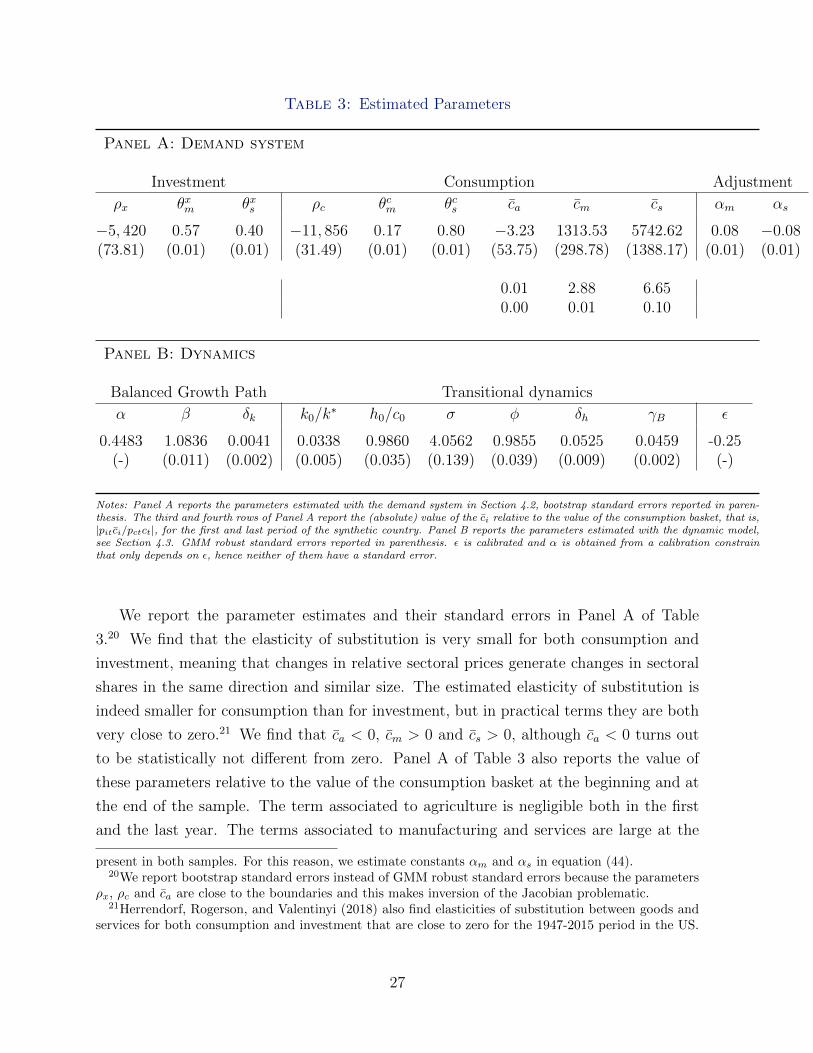
Table 3: Estimated Parameters
Panel A: Demand system
Investment Consumption Adjustment
ρx θxm θxs ρc θcm θcs ca cm cs αm αs
−5, 420 0.57 0.40 −11, 856 0.17 0.80 −3.23 1313.53 5742.62 0.08 −0.08(73.81) (0.01) (0.01) (31.49) (0.01) (0.01) (53.75) (298.78) (1388.17) (0.01) (0.01)
0.01 2.88 6.650.00 0.01 0.10
Panel B: Dynamics
Balanced Growth Path Transitional dynamics
α β δk k0/k∗ h0/c0 σ φ δh γB ε
0.4483 1.0836 0.0041 0.0338 0.9860 4.0562 0.9855 0.0525 0.0459 -0.25(-) (0.011) (0.002) (0.005) (0.035) (0.139) (0.039) (0.009) (0.002) (-)
Notes: Panel A reports the parameters estimated with the demand system in Section 4.2, bootstrap standard errors reported in paren-thesis. The third and fourth rows of Panel A report the (absolute) value of the ci relative to the value of the consumption basket, that is,|pitci/pctct|, for the first and last period of the synthetic country. Panel B reports the parameters estimated with the dynamic model,see Section 4.3. GMM robust standard errors reported in parenthesis. ε is calibrated and α is obtained from a calibration constrainthat only depends on ε, hence neither of them have a standard error.
We report the parameter estimates and their standard errors in Panel A of Table
3.20 We find that the elasticity of substitution is very small for both consumption and
investment, meaning that changes in relative sectoral prices generate changes in sectoral
shares in the same direction and similar size. The estimated elasticity of substitution is
indeed smaller for consumption than for investment, but in practical terms they are both
very close to zero.21 We find that ca < 0, cm > 0 and cs > 0, although ca < 0 turns out
to be statistically not different from zero. Panel A of Table 3 also reports the value of
these parameters relative to the value of the consumption basket at the beginning and at
the end of the sample. The term associated to agriculture is negligible both in the first
and the last year. The terms associated to manufacturing and services are large at the
present in both samples. For this reason, we estimate constants αm and αs in equation (44).20We report bootstrap standard errors instead of GMM robust standard errors because the parameters
ρx, ρc and ca are close to the boundaries and this makes inversion of the Jacobian problematic.21Herrendorf, Rogerson, and Valentinyi (2018) also find elasticities of substitution between goods and
services for both consumption and investment that are close to zero for the 1947-2015 period in the US.
27
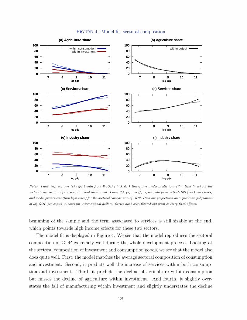
Figure 4: Model fit, sectoral composition
0
20
40
60
80
100
7 8 9 10 11log gdp
(a) Agriculture share
within consumptionwithin investment
0
20
40
60
80
100
7 8 9 10 11log gdp
(a) Agriculture share
0
20
40
60
80
100
7 8 9 10 11log gdp
(a) Agriculture share
0
20
40
60
80
100
7 8 9 10 11log gdp
(a) Agriculture share
0
20
40
60
80
100
7 8 9 10 11log gdp
(a) Agriculture share
0
20
40
60
80
100
7 8 9 10 11log gdp
(b) Agriculture share
within output
0
20
40
60
80
100
7 8 9 10 11log gdp
(b) Agriculture share
0
20
40
60
80
100
7 8 9 10 11log gdp
(b) Agriculture share
0
20
40
60
80
100
7 8 9 10 11log gdp
(c) Services share
0
20
40
60
80
100
7 8 9 10 11log gdp
(c) Services share
0
20
40
60
80
100
7 8 9 10 11log gdp
(c) Services share
0
20
40
60
80
100
7 8 9 10 11log gdp
(c) Services share
0
20
40
60
80
100
7 8 9 10 11log gdp
(d) Services share
0
20
40
60
80
100
7 8 9 10 11log gdp
(d) Services share
0
20
40
60
80
100
7 8 9 10 11log gdp
(e) Industry share
0
20
40
60
80
100
7 8 9 10 11log gdp
(e) Industry share
0
20
40
60
80
100
7 8 9 10 11log gdp
(e) Industry share
0
20
40
60
80
100
7 8 9 10 11log gdp
(e) Industry share
0
20
40
60
80
100
7 8 9 10 11log gdp
(e) Industry share
0
20
40
60
80
100
7 8 9 10 11log gdp
(f) Industry share
0
20
40
60
80
100
7 8 9 10 11log gdp
(f) Industry share
Notes. Panel (a), (c) and (e) report data from WIOD (thick dark lines) and model predictions (thin light lines) for the
sectoral composition of consumption and investment. Panel (b), (d) and (f) report data from WDI-G10S (thick dark lines)
and model predictions (thin light lines) for the sectoral composition of GDP. Data are projections on a quadratic polynomial
of log GDP per capita in constant international dollars. Series have been filtered out from country fixed effects.
beginning of the sample and the term associated to services is still sizable at the end,
which points towards high income effects for these two sectors.
The model fit is displayed in Figure 4. We see that the model reproduces the sectoral
composition of GDP extremely well during the whole development process. Looking at
the sectoral composition of investment and consumption goods, we see that the model also
does quite well. First, the model matches the average sectoral composition of consumption
and investment. Second, it predicts well the increase of services within both consump-
tion and investment. Third, it predicts the decline of agriculture within consumption
but misses the decline of agriculture within investment. And fourth, it slightly over-
states the fall of manufacturing within investment and slightly understates the decline
28
of manufacturing within consumption, creating a small hump of manufacturing within
consumption that is absent in the WIOD. The reason for this latter result is that the
increase of manufacturing within GDP in the early stages of development measured in
the WDI-G10S data set is very sharp and cannot be completely accounted by the ob-
served increase in the investment rate. Hence, the estimation requires a slight increase of
manufacturing within consumption and/or investment, which is achieved by an income
elasticity of manufacturing within consumption larger than one at the beginning of the
development process.
In order to assess the relative importance of each mechanism of structural change, we
re-evaluate equation (33) in a series of counterfactual exercises that we plot in Panels (a)
to (c) of Figure 5. First, we set ρx = ρc = 0 and ci = 0 such that the sectoral composition
within consumption and investment is constant and hence the only source of structural
change is the change in the investment rate, that is, the extensive margin (see the thick
yellow lines). Second, we activate the estimated ρx, ρc, and ci but set the investment
rate constant such that we isolate the structural change coming from the intensive margin
(thick dark blue lines). These two exercises show how the overall trends in agriculture and
services are roughly well captured by the standard mechanisms operating in the intensive
margin. However, when looking at the evolution of the share of manufacturing in GDP
we see that both the intensive and the extensive margins matter to generate the hump.
With the sectoral composition of investment and consumption goods held constant, the
change in the investment rate produces and increase in the share of manufactures of
15.1 percentage points (as compared to 24.0 in the data) and a decline afterwards of
6.9 (as compared to 11.2 in the data). With the investment rate held constant, the
change in the sectoral composition within consumption and investment produces a hump
in manufacturing similar in shape and size to the one produced by the changes in the
investment rate.
Finally, we perform two more exercises to separate the different channels operating in
the intensive margin. First, we set ρx = ρc = 0 and hold the investment rate constant
such that we produce structural change coming from income effects only (thin dark blue
lines), and second we set ci = 0 also holding the investment rate constant such that we
isolate changes in sectoral composition coming from relative price effects only (thin gray
lines).22 We note that the price of services relative to the price of manufactures increases
22When we set the investment rate constant we choose the average of the time series. When we changeρx, ρc, or ci = 0 we re-calibrate θxi and θci to match the average sectoral shares within investment andconsumption. Finally, for ease of exposition we add or subtract a constant to the counterfactual timesseries such that they all start at the same level as the baseline.
29
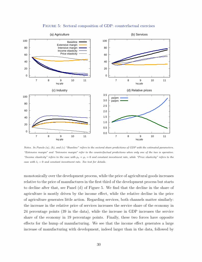
Figure 5: Sectoral composition of GDP: counterfactual exercises
0
20
40
60
80
100
7 8 9 10 11log gdp
(a) Agriculture
BaselineExtensive marginIntensive marginIncome elasticity
Price elasticity
0
20
40
60
80
100
7 8 9 10 11log gdp
(b) Services
0
20
40
60
80
100
7 8 9 10 11log gdp
(c) Industry
0.0
0.5
1.0
1.5
2.0
2.5
3.0
3.5
7 8 9 10 11log gdp
(d) Relative prices
ps/pmpa/pm
Notes. In Panels (a), (b), and (c) “Baseline” refers to the sectoral share predictions of GDP with the estimated parameters.
“Extensive margin” and “Intensive margin” refer to the counterfactual predictions when only one of the two is operative.
“Income elasitcity” refers to the case with ρx = ρc = 0 and constant investment rate, while “Price elasticity” refers to the
case with ci = 0 and constant investment rate. See test for details.
monotonically over the development process, while the price of agricultural goods increases
relative to the price of manufactures in the first third of the development process but starts
to decline after that, see Panel (d) of Figure 5. We find that the decline in the share of
agriculture is mostly driven by the income effect, while the relative decline in the price
of agriculture generates little action. Regarding services, both channels matter similarly:
the increase in the relative price of services increases the service share of the economy in
24 percentage points (39 in the data), while the increase in GDP increases the service
share of the economy in 19 percentage points. Finally, these two forces have opposite
effects for the hump of manufacturing. We see that the income effect generates a large
increase of manufacturing with development, indeed larger than in the data, followed by
30
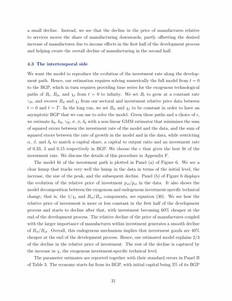
a small decline. Instead, we see that the decline in the price of manufactures relative
to services moves the share of manufacturing downwards, partly offsetting the desired
increase of manufactures due to income effects in the first half of the development process
and helping create the overall decline of manufacturing in the second half.
4.3 The intertemporal side
We want the model to reproduce the evolution of the investment rate along the develop-
ment path. Hence, our estimation requires solving numerically the full model from t = 0
to the BGP, which in turn requires providing time series for the exogenous technological
paths of Bt, Bit, and χt from t = 0 to infinity. We set Bt to grow at a constant rate
γB, and recover Bit and χt from our sectoral and investment relative price data between
t = 0 and t = T . In the long run, we set Bit and χt to be constant in order to have an
asymptotic BGP that we can use to solve the model. Given these paths and a choice of ε,
we estimate k0, h0, γB, σ, φ, δh with a non-linear GMM estimator that minimizes the sum
of squared errors between the investment rate of the model and the data, and the sum of
squared errors between the rate of growth in the model and in the data, while restricting
α, β, and δk to match a capital share, a capital to output ratio and an investment rate
of 0.33, 3 and 0.15 respectively in BGP. We choose the ε that gives the best fit of the
investment rate. We discuss the details of this procedure in Appendix F.
The model fit of the investment path is plotted in Panel (a) of Figure 6. We see a
clear hump that tracks very well the hump in the data in terms of the initial level, the
increase, the size of the peak, and the subsequent decline. Panel (b) of Figure 6 displays
the evolution of the relative price of investment pxt/pct in the data. It also shows the
model decomposition between the exogenous and endogenous investment-specific technical
change, that is, the 1/χt and Bct/Bxt components, see equation (30). We see how the
relative price of investment is more or less constant in the first half of the development
process and starts to decline after that, with investment becoming 60% cheaper at the
end of the development process. The relative decline of the price of manufactures coupled
with the larger importance of manufactures within investment generates a smooth decline
of Bct/Bxt. Overall, this endogenous mechanism implies that investment goods are 40%
cheaper at the end of the development process. Hence, our estimated model explains 2/3
of the decline in the relative price of investment. The rest of the decline is captured by
the increase in χ, the exogenous investment-specific technical level.
The parameter estimates are reported together with their standard errors in Panel B
of Table 3. The economy starts far from its BGP, with initial capital being 3% of its BGP
31
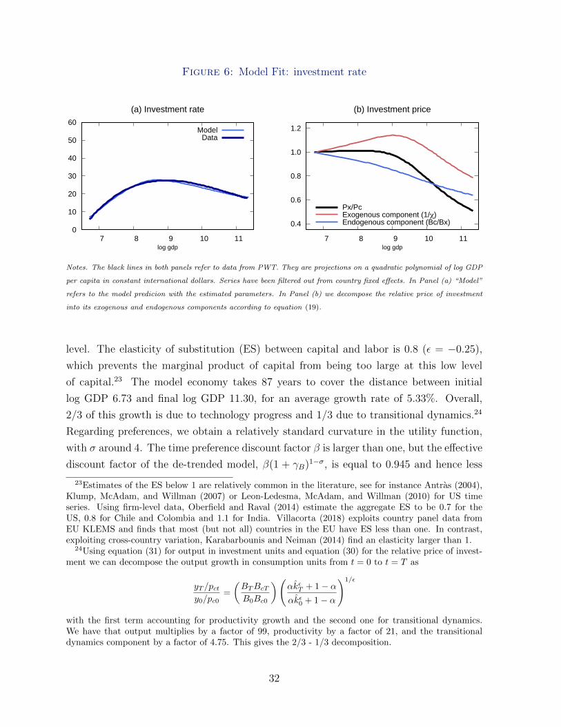
Figure 6: Model Fit: investment rate
0
10
20
30
40
50
60
7 8 9 10 11log gdp
(a) Investment rate
ModelData
0.4
0.6
0.8
1.0
1.2
7 8 9 10 11log gdp
(b) Investment price
Px/PcExogenous component (1/χ)Endogenous component (Bc/Bx)
Notes. The black lines in both panels refer to data from PWT. They are projections on a quadratic polynomial of log GDP
per capita in constant international dollars. Series have been filtered out from country fixed effects. In Panel (a) “Model”
refers to the model predicion with the estimated parameters. In Panel (b) we decompose the relative price of investment
into its exogenous and endogenous components according to equation (19).
level. The elasticity of substitution (ES) between capital and labor is 0.8 (ε = −0.25),
which prevents the marginal product of capital from being too large at this low level
of capital.23 The model economy takes 87 years to cover the distance between initial
log GDP 6.73 and final log GDP 11.30, for an average growth rate of 5.33%. Overall,
2/3 of this growth is due to technology progress and 1/3 due to transitional dynamics.24
Regarding preferences, we obtain a relatively standard curvature in the utility function,
with σ around 4. The time preference discount factor β is larger than one, but the effective
discount factor of the de-trended model, β(1 + γB)1−σ, is equal to 0.945 and hence less
23Estimates of the ES below 1 are relatively common in the literature, see for instance Antras (2004),Klump, McAdam, and Willman (2007) or Leon-Ledesma, McAdam, and Willman (2010) for US timeseries. Using firm-level data, Oberfield and Raval (2014) estimate the aggregate ES to be 0.7 for theUS, 0.8 for Chile and Colombia and 1.1 for India. Villacorta (2018) exploits country panel data fromEU KLEMS and finds that most (but not all) countries in the EU have ES less than one. In contrast,exploiting cross-country variation, Karabarbounis and Neiman (2014) find an elasticity larger than 1.
24Using equation (31) for output in investment units and equation (30) for the relative price of invest-ment we can decompose the output growth in consumption units from t = 0 to t = T as
yT /pcty0/pc0
=
(BTBcTB0Bc0
)(αkεT + 1− ααkε0 + 1− α
)1/ε
with the first term accounting for productivity growth and the second one for transitional dynamics.We have that output multiplies by a factor of 99, productivity by a factor of 21, and the transitionaldynamics component by a factor of 4.75. This gives the 2/3 - 1/3 decomposition.
32
than one. The estimated parameters of the habit process imply that the habit stock
at the beginning of the transition is large, 98% of consumption. This feature, together
with the large weight of habit in the utility function (φ = 0.9855), is required to match
the relatively low initial investment rate, when capital is low and hence the returns to
investment are high. Finally, we need the habit process to be persistent, with δh = 0.0525,
to match the timing of the investment peak. A low δh is consistent with the idea of a
slow-moving reference level of consumption.
4.4 Counterfactual exercises
We want to to understand the joint determination of the investment rate and the sectoral
composition of the economy along the development path. Our model has three exoge-
nous sources of technology change: aggregate productivity, asymmetric sector-specific
technology, and investment-specific technical level. In addition, it features endogenous
transitional dynamics arising from the low initial capital stock. All these elements can
potentially shape the paths of investment and sectoral composition. First, aggregate
productivity growth and transitional dynamics make the economy richer and drive struc-
tural change in the intensive margin through the non-unitary income elasticity. They
also affect the investment rate through the interplay of the income and substitution ef-
fect present in the standard one-sector neo-classical growth model, and hence drive the
extensive margin of structural change. Second, the asymmetric sector-specific produc-
tivity growth affects the intensive margin of structural change through the non-unitary
elasticity of substitution. It also affects the investment rate through the induced changes
in the endogenous component of the relative price of investment, and hence the extensive
margin of structural change. Finally, the investment-specific technical change affects the
investment rate, and because of this it affects the extensive margin of structural change.
It also has a negligible effect on the intensive margin, as changes in the investment rate
change total consumption expenditure for a given income level and hence interact with
the non-homotheticities within consumption.
In order to assess the relative importance of these mechanisms, we solve for the follow-
ing two simple counterfactual economies. First, we set γBat = γBst = γBmt = γBmt ∀t in
order to have an economy where the relative sectoral prices are constant, and choose γBmt
such that the counterfactual economy displays the same path of the Hicks-neutral tech-
nical change of GDP as in the benchmark economy.25 We call this economy E1. Second,
25We can define the Hicks-neutral technical level of GDP Byt as the weighted average of the Hicks-neutral technical level in investment and consumption, Byt ≡ Bxtχtpxtxt/yt+Bct (1− pxtxt/yt). Keepingthe same investment rate as in the benchmark economy we can recover the time path of γBmt that
33
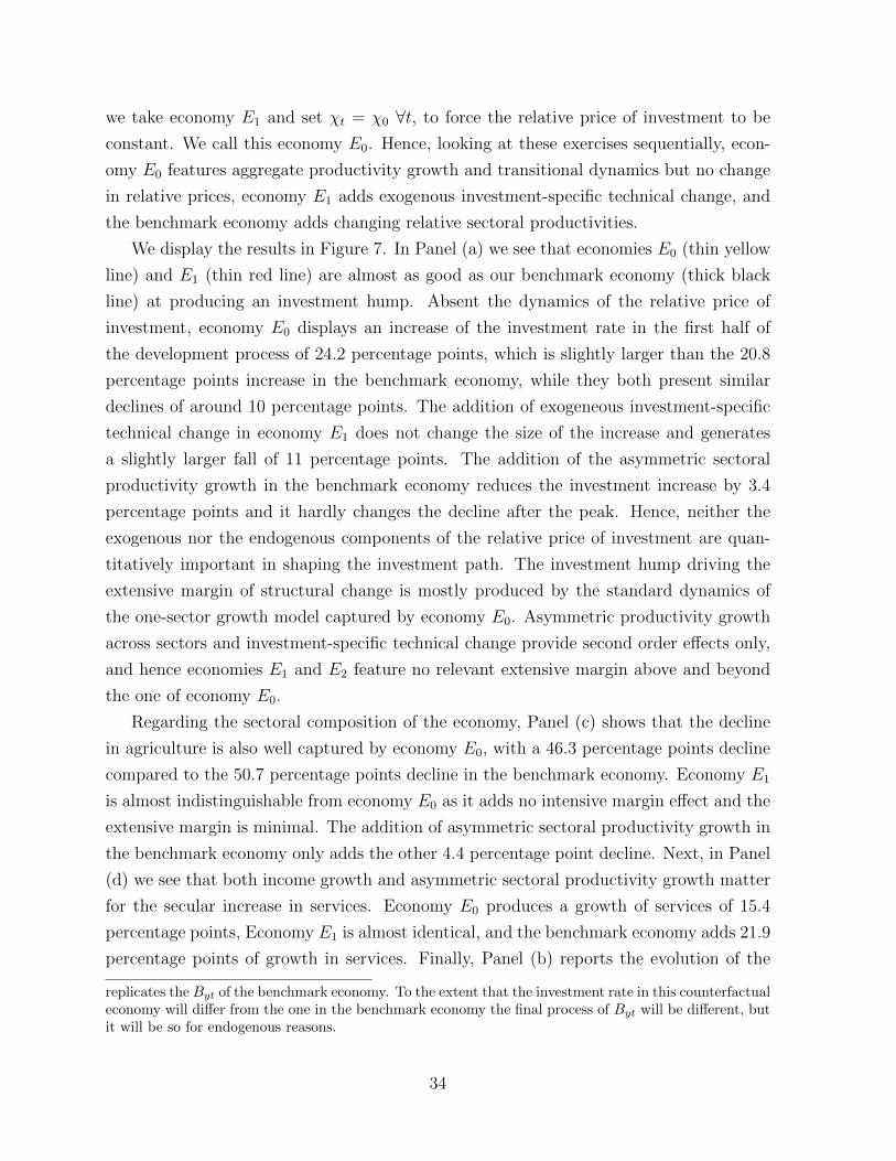
we take economy E1 and set χt = χ0 ∀t, to force the relative price of investment to be
constant. We call this economy E0. Hence, looking at these exercises sequentially, econ-
omy E0 features aggregate productivity growth and transitional dynamics but no change
in relative prices, economy E1 adds exogenous investment-specific technical change, and
the benchmark economy adds changing relative sectoral productivities.
We display the results in Figure 7. In Panel (a) we see that economies E0 (thin yellow
line) and E1 (thin red line) are almost as good as our benchmark economy (thick black
line) at producing an investment hump. Absent the dynamics of the relative price of
investment, economy E0 displays an increase of the investment rate in the first half of
the development process of 24.2 percentage points, which is slightly larger than the 20.8
percentage points increase in the benchmark economy, while they both present similar
declines of around 10 percentage points. The addition of exogeneous investment-specific
technical change in economy E1 does not change the size of the increase and generates
a slightly larger fall of 11 percentage points. The addition of the asymmetric sectoral
productivity growth in the benchmark economy reduces the investment increase by 3.4
percentage points and it hardly changes the decline after the peak. Hence, neither the
exogenous nor the endogenous components of the relative price of investment are quan-
titatively important in shaping the investment path. The investment hump driving the
extensive margin of structural change is mostly produced by the standard dynamics of
the one-sector growth model captured by economy E0. Asymmetric productivity growth
across sectors and investment-specific technical change provide second order effects only,
and hence economies E1 and E2 feature no relevant extensive margin above and beyond
the one of economy E0.
Regarding the sectoral composition of the economy, Panel (c) shows that the decline
in agriculture is also well captured by economy E0, with a 46.3 percentage points decline
compared to the 50.7 percentage points decline in the benchmark economy. Economy E1
is almost indistinguishable from economy E0 as it adds no intensive margin effect and the
extensive margin is minimal. The addition of asymmetric sectoral productivity growth in
the benchmark economy only adds the other 4.4 percentage point decline. Next, in Panel
(d) we see that both income growth and asymmetric sectoral productivity growth matter
for the secular increase in services. Economy E0 produces a growth of services of 15.4
percentage points, Economy E1 is almost identical, and the benchmark economy adds 21.9
percentage points of growth in services. Finally, Panel (b) reports the evolution of the
replicates the Byt of the benchmark economy. To the extent that the investment rate in this counterfactualeconomy will differ from the one in the benchmark economy the final process of Byt will be different, butit will be so for endogenous reasons.
34
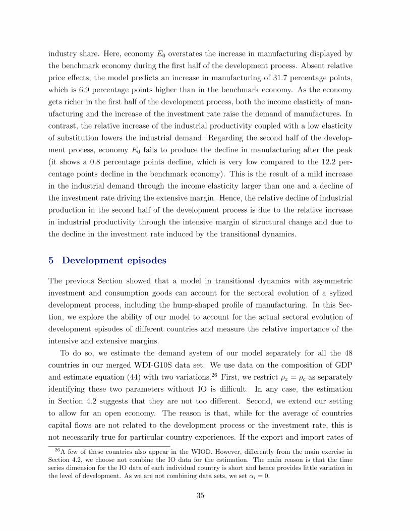
industry share. Here, economy E0 overstates the increase in manufacturing displayed by
the benchmark economy during the first half of the development process. Absent relative
price effects, the model predicts an increase in manufacturing of 31.7 percentage points,
which is 6.9 percentage points higher than in the benchmark economy. As the economy
gets richer in the first half of the development process, both the income elasticity of man-
ufacturing and the increase of the investment rate raise the demand of manufactures. In
contrast, the relative increase of the industrial productivity coupled with a low elasticity
of substitution lowers the industrial demand. Regarding the second half of the develop-
ment process, economy E0 fails to produce the decline in manufacturing after the peak
(it shows a 0.8 percentage points decline, which is very low compared to the 12.2 per-
centage points decline in the benchmark economy). This is the result of a mild increase
in the industrial demand through the income elasticity larger than one and a decline of
the investment rate driving the extensive margin. Hence, the relative decline of industrial
production in the second half of the development process is due to the relative increase
in industrial productivity through the intensive margin of structural change and due to
the decline in the investment rate induced by the transitional dynamics.
5 Development episodes
The previous Section showed that a model in transitional dynamics with asymmetric
investment and consumption goods can account for the sectoral evolution of a sylized
development process, including the hump-shaped profile of manufacturing. In this Sec-
tion, we explore the ability of our model to account for the actual sectoral evolution of
development episodes of different countries and measure the relative importance of the
intensive and extensive margins.
To do so, we estimate the demand system of our model separately for all the 48
countries in our merged WDI-G10S data set. We use data on the composition of GDP
and estimate equation (44) with two variations.26 First, we restrict ρx = ρc as separately
identifying these two parameters without IO is difficult. In any case, the estimation
in Section 4.2 suggests that they are not too different. Second, we extend our setting
to allow for an open economy. The reason is that, while for the average of countries
capital flows are not related to the development process or the investment rate, this is
not necessarily true for particular country experiences. If the export and import rates of
26A few of these countries also appear in the WIOD. However, differently from the main exercise inSection 4.2, we choose not combine the IO data for the estimation. The main reason is that the timeseries dimension for the IO data of each individual country is short and hence provides little variation inthe level of development. As we are not combining data sets, we set αi = 0.
35
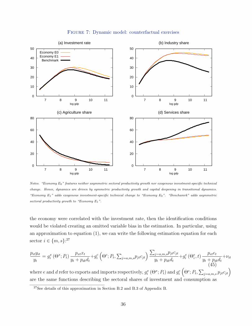
Figure 7: Dynamic model: counterfactual exercises
0
10
20
30
40
50
7 8 9 10 11log gdp
(a) Investment rate
Economy E0Economy E1
Benchmark
0
10
20
30
40
50
7 8 9 10 11log gdp
(b) Industry share
0
20
40
60
80
7 8 9 10 11log gdp
(c) Agriculture share
0
20
40
60
80
7 8 9 10 11log gdp
(d) Services share
Notes. “Economy E0” features neither asymmetric sectoral productivity growth nor exogenous investment-specific technical
change. Hence, dynamics are driven by symmetric productivity growth and capital deepening in transitional dynamics.
“Economy E1” adds exogenous investment-specific technical change to “Economy E0”. “Benchamrk” adds asymmetric
sectoral productivity growth to “Economy E1”.
the economy were correlated with the investment rate, then the identification conditions
would be violated creating an omitted variable bias in the estimation. In particular, using
an approximation to equation (1), we can write the following estimation equation for each
sector i ∈ {m, s}:27
pityityt
= gxi (Θx;Pt)pxtxt
yt + pdtdt+gci
(Θc;Pt,
∑j=a,m,spjtcjt
) ∑j=a,m,spjtcjt
yt + pdtdt+gei (Θe
i , t)petet
yt + pdtdt+νit
(45)
where e and d refer to exports and imports respectively, gxi (Θx;Pt) and gci
(Θc;Pt,
∑j=a,m,s pjtcjt
)are the same functions describing the sectoral shares of investment and consumption as
27See details of this approximation in Section B.2 and B.3 of Appendix B.
36

in equation (44), and the function gei (Θei , t) captures the value added share of exports.
In our estimation approach we model the sectoral value added shares of exports in each
country as a logistic function that depends on a country-specific low order polynomial on
calendar time.28 Finally, νit ≡ petetyt+pdtdt
εeit + εyit is the econometric error, with εeit reflect-
ing idiosyncratic variation in export shares that is not captured by the country-specific
time trends of our reduced-form modeling of the sectoral composition of exports and εyitis measurement error as in equation (44). A non-linear estimator that exploits moment
conditions like E[νit|Pt,
∑jpjtcjt,
pxtxtyt+pdtdt
, petetyt+pdtdt
]= 0 will deliver consistent estimates
of the parameters. Hence, the identifying assumption is that deviations from the trend
in sectoral export shares (εeit) are uncorrelated with sectoral prices, consumption expen-
diture, and the investment and export rates.29 We estimate the model in a Bayesian
fashion and use Markov Chain Monte Carlo methods (MCMC) for computation. We use
flat priors (non-informative priors) in order to obtain results which should be as in the
GMM framework. We give full details of the estimation in Appendix G.
5.1 Estimation results
The estimated parameters and their standard errors for each country are reported in
Table G.2 in Appendix G. In here, we will focus on the consequences for the sectoral
composition of GDP, consumption, and investment. The first result to highlight is that
the estimated model matches the evolution of the sectoral composition of GDP in each
country very well, see Appendix G.30
Second, we recover a substantial asymmetry between investment and consumption
goods. The first row in Table 4 reports the model-implied sectoral composition of each
good when taking the average over all countries and years. We see that the share of
manufactures in investment goods is 37.0 percentage points larger than in consumption
28We model these sectoral shares as logistic functions to ensure that the shares lie between 0 and 1. Amore parsimonious approach would have been to model the sectoral composition of exports as constant;however, the composition of exports typically changes with development, so to better fit the data weallow these sectoral compositions to vary over time.
29Also note that equation (45) presents conditional heteroskedasticity by construction since
var(νit|Pt,
∑jpjtcjt,
pxtxt
yt+pdtdt, petetyt+pdtdt
)= var (εeit)×
(petet
yt + pdtdt
)2
+ var (εyit)
We use White standard errors, which are robust to any kind of conditional heteroskedasticity.30In particular, regressing the sectoral shares in the data against their model predictions gives intercepts
close to zero, slopes close to one, and R2 around 97% for the three sectors, see Figure G.1. The modelfit country by country is also good: Table G.1 reports the fit country by country for each sector, whilePanel (a) in Figures G.2-G.49 plots the actual and model-implied time series of the value added share ofmanufacturing for each country.
37

goods (column 8). This figure is remarkably similar to the 39.4 percentage points measured
in the WIOD (see Table 1), which is a good validation of our estimation strategy as no
information from IO data has been used in the estimation. However, the countries and
years used in the estimation differ from the ones in WIOD. For this reason, we report
the sectoral composition of consumption and investment for the common countries and
years in our estimation sample and in the WIOD, this is 25 countries in the period
1995 to 2011 (see the second and third rows of Table 4). We find that the mean of our
estimates resemble the data in the WIOD reasonably well: the share of manufactures
is 37.5 percentage points higher in investment than in consumption in the WIOD data,
while this difference is 42.4 percentage points in our estimation. When comparing the
model predictions with the WIOD data country by country, we see that our estimation
does a good job in predicting the sectoral composition of investment and consumption
goods for a reasonably high number of countries. For instance, in terms of the different
share of manufacturing within investment and consumption goods, the difference between
the model and data is less than 5 percentage points for 9 countries (Austria, Hungary,
Indonesia, Netherlands, Portugal, South Korea, Taiwan, UK, and the US) and less 10
percentage points for other 4 countries (Brazil, China, India, and Turkey).31
Third, the predicted evolution of the sectoral shares of output, consumption, and
investment is consistent with the evidence we have in the data. In particular, Figure 8
plots the evolution of the estimated share of manufactures for the whole economy and for
the investment and consumption goods against the level of development, after filtering
out cross-country differences in levels. We observe a mild hump in consumption but not
in investment, see Panel (c) and (d) respectively. The estimated model also produces
a larger hump of manufacturing in GDP, see Panel (b), which resembles very much the
one in the data, see Panel (a). This is the same pattern we uncovered with the panel of
countries estimation including IO data (which we do not use here), and not too different
from what we find in the WIOD data in Figure 2. In addition, and not reported here, we
also find a larger fall of agriculture and a larger increase of services within consumption
than within investment as in the WIOD data.
Finally, we can evaluate the predictions of our model for the case of the US against
the available long time series of the IO tables. We find that our model does qualitatively
well in predicting the long run trends of the structural transformation happening in the
intensive margin, although quantitatively it misses part of the changes. For example,
31See Panel (d) in Figures G.2-G.49 of Appendix G for more details on the model-implied and WIODtime series of the value added share of manufacturing within investment and consumption country bycountry.
38
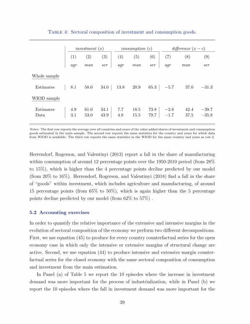
Table 4: Sectoral composition of investment and consumption goods.
investment (x) consumption (c) difference (x− c)
(1) (2) (3) (4) (5) (6) (7) (8) (9)
agr man ser agr man ser agr man ser
Whole sample
Estimates 8.1 58.0 34.0 13.8 20.9 65.3 −5.7 37.0 −31.3
WIOD sample
Estimates 4.9 61.0 34.1 7.7 18.5 73.8 −2.8 42.4 −39.7Data 3.1 53.0 43.9 4.8 15.5 79.7 −1.7 37.5 −35.8
Notes: The first row reports the average over all countries and years of the value added shares of investment and consumptiongoods estimated in the main sample. The second row reports the same statistics for the country and years for which datafrom WIOD is available. The third row reports the same statistics in the WIOD for the same country and years as row 2.
Herrendorf, Rogerson, and Valentinyi (2013) report a fall in the share of manufacturing
within consumption of around 12 percentage points over the 1950-2010 period (from 28%
to 15%), which is higher than the 4 percentage points decline predicted by our model
(from 20% to 16%). Herrendorf, Rogerson, and Valentinyi (2018) find a fall in the share
of “goods” within investment, which includes agriculture and manufacturing, of around
15 percentage points (from 65% to 50%), which is again higher than the 5 percentage
points decline predicted by our model (from 62% to 57%) .
5.2 Accounting exercises
In order to quantify the relative importance of the extensive and intensive margins in the
evolution of sectoral composition of the economy we perform two different decompositions.
First, we use equation (45) to produce for every country counterfactual series for the open
economy case in which only the intensive or extensive margins of structural change are
active. Second, we use equation (44) to produce intensive and extensive margin counter-
factual series for the closed economy with the same sectoral composition of consumption
and investment from the main estimation.
In Panel (a) of Table 5 we report the 10 episodes where the increase in investment
demand was more important for the process of industrialization, while in Panel (b) we
report the 10 episodes where the fall in investment demand was more important for the
39
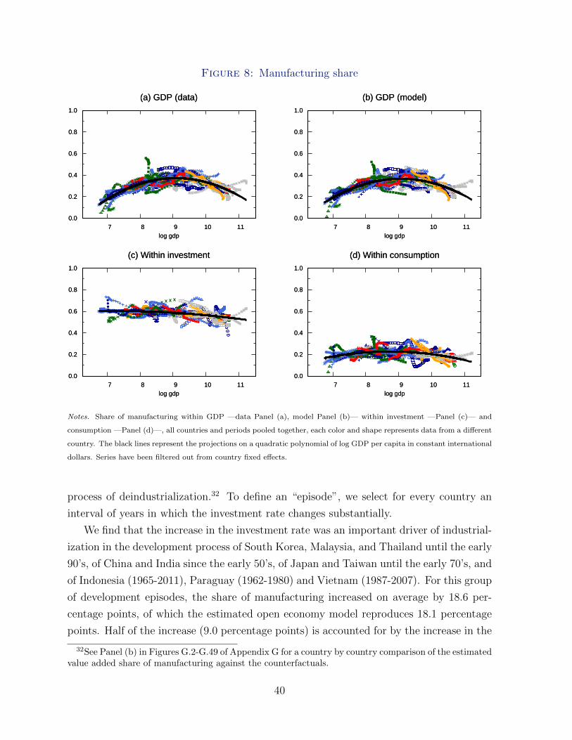
Figure 8: Manufacturing share
0.0
0.2
0.4
0.6
0.8
1.0
7 8 9 10 11log gdp
(a) GDP (data)
0.0
0.2
0.4
0.6
0.8
1.0
7 8 9 10 11log gdp
(a) GDP (data)
0.0
0.2
0.4
0.6
0.8
1.0
7 8 9 10 11log gdp
(b) GDP (model)
0.0
0.2
0.4
0.6
0.8
1.0
7 8 9 10 11log gdp
(b) GDP (model)
0.0
0.2
0.4
0.6
0.8
1.0
7 8 9 10 11log gdp
(c) Within investment
0.0
0.2
0.4
0.6
0.8
1.0
7 8 9 10 11log gdp
(c) Within investment
0.0
0.2
0.4
0.6
0.8
1.0
7 8 9 10 11log gdp
(d) Within consumption
0.0
0.2
0.4
0.6
0.8
1.0
7 8 9 10 11log gdp
(d) Within consumption
Notes. Share of manufacturing within GDP —data Panel (a), model Panel (b)— within investment —Panel (c)— and
consumption —Panel (d)—, all countries and periods pooled together, each color and shape represents data from a different
country. The black lines represent the projections on a quadratic polynomial of log GDP per capita in constant international
dollars. Series have been filtered out from country fixed effects.
process of deindustrialization.32 To define an “episode”, we select for every country an
interval of years in which the investment rate changes substantially.
We find that the increase in the investment rate was an important driver of industrial-
ization in the development process of South Korea, Malaysia, and Thailand until the early
90’s, of China and India since the early 50’s, of Japan and Taiwan until the early 70’s, and
of Indonesia (1965-2011), Paraguay (1962-1980) and Vietnam (1987-2007). For this group
of development episodes, the share of manufacturing increased on average by 18.6 per-
centage points, of which the estimated open economy model reproduces 18.1 percentage
points. Half of the increase (9.0 percentage points) is accounted for by the increase in the
32See Panel (b) in Figures G.2-G.49 of Appendix G for a country by country comparison of the estimatedvalue added share of manufacturing against the counterfactuals.
40
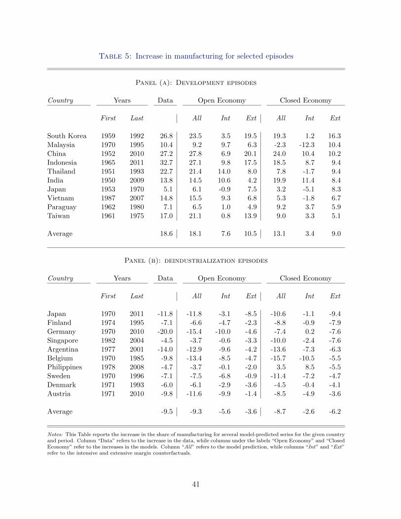
Table 5: Increase in manufacturing for selected episodes
Panel (a): Development episodes
Country Years Data Open Economy Closed Economy
First Last All Int Ext All Int Ext
South Korea 1959 1992 26.8 23.5 3.5 19.5 19.3 1.2 16.3Malaysia 1970 1995 10.4 9.2 9.7 6.3 -2.3 -12.3 10.4China 1952 2010 27.2 27.8 6.9 20.1 24.0 10.4 10.2Indonesia 1965 2011 32.7 27.1 9.8 17.5 18.5 8.7 9.4Thailand 1951 1993 22.7 21.4 14.0 8.0 7.8 -1.7 9.4India 1950 2009 13.8 14.5 10.6 4.2 19.9 11.4 8.4Japan 1953 1970 5.1 6.1 -0.9 7.5 3.2 -5.1 8.3Vietnam 1987 2007 14.8 15.5 9.3 6.8 5.3 -1.8 6.7Paraguay 1962 1980 7.1 6.5 1.0 4.9 9.2 3.7 5.9Taiwan 1961 1975 17.0 21.1 0.8 13.9 9.0 3.3 5.1
Average 18.6 18.1 7.6 10.5 13.1 3.4 9.0
Panel (b): deindustrialization episodes
Country Years Data Open Economy Closed Economy
First Last All Int Ext All Int Ext
Japan 1970 2011 -11.8 -11.8 -3.1 -8.5 -10.6 -1.1 -9.4Finland 1974 1995 -7.1 -6.6 -4.7 -2.3 -8.8 -0.9 -7.9Germany 1970 2010 -20.0 -15.4 -10.0 -4.6 -7.4 0.2 -7.6Singapore 1982 2004 -4.5 -3.7 -0.6 -3.3 -10.0 -2.4 -7.6Argentina 1977 2001 -14.0 -12.9 -9.6 -4.2 -13.6 -7.3 -6.3Belgium 1970 1985 -9.8 -13.4 -8.5 -4.7 -15.7 -10.5 -5.5Philippines 1978 2008 -4.7 -3.7 -0.1 -2.0 3.5 8.5 -5.5Sweden 1970 1996 -7.1 -7.5 -6.8 -0.9 -11.4 -7.2 -4.7Denmark 1971 1993 -6.0 -6.1 -2.9 -3.6 -4.5 -0.4 -4.1Austria 1971 2010 -9.8 -11.6 -9.9 -1.4 -8.5 -4.9 -3.6
Average -9.5 -9.3 -5.6 -3.6 -8.7 -2.6 -6.2
Notes: This Table reports the increase in the share of manufacturing for several model-predicted series for the given countryand period. Column “Data” refers to the increase in the data, while columns under the labels “Open Economy” and “ClosedEconomy” refer to the increases in the models. Column “All” refers to the model prediction, while columns “Int” and “Ext”refer to the intensive and extensive margin counterfactuals.
41
investment rate (the extensive margin of the closed economy), while only 1/5 (3.4 percent-
age points) by the increase in manufacturing within investment and within consumption
(the intensive margin of the closed economy). Overall, the closed economy explains an
increase of 13.1 percentage points, leaving less than 1/3 to be explained by the increase
in the level and composition of exports.
In the case of South Korea, for example, there was an increase in the share of manufac-
turing of 26.8 percentage points between 1959 and 1992. Our estimated model accounts
for 23.5 points increase, of which 3.5 percentage points come from the intensive margin
and 19.5 come from the extensive margin. When restricting the analysis to the closed
economy case our model produces an increase in industrial value added of 19.3 percentage
points, 1.2 from the intensive margin and 16.3 from the extensive margin. We note that
the closed economy exercise under-predicts the increase in manufacturing by 4 percentage
points, which is due to both the intensive and extensive margins. The larger increase of
the intensive margin in the open economy (3.5 percentage points vs. 1.2 in the closed
economy) reflects that there was a faster increase of manufactures within exports than
within domestic demand. The larger increase of the extensive margin in the open economy
economy (19.5 percentage points vs. 16.3 in the closed economy) reflects a large increase
in exports (from 2 to 25 percent of GDP) and the fact that in South Korea exports were
more intensive in value added from manufacturing than domestic demand. But all in
all, the sustained increase in the investment rate in South Korea over this period was a
fundamental driver of its industrialization process.33
Next, we also find investment to be an important driver of structural change in many
countries that went through a deindustrialization process in the 70’s or the 80’s. In
particular, this was the case in Japan, Finland, Germany, Sweden, Denmark, and Austria
since the early 70’s or Singapore, Philippines and Argentina since the late 70’s or early
80’s. On average, these countries saw a decline in manufactures of 9.5 percentage points,
of which 2/3 (6.2 percentage points) come from the decline of the investment rate, 1/4
(2.6 percentage points) from the decline of manufacturing within domestic demand, and
the rest from changes in the level and composition of exports.
For a particular example we can focus on Germany. The share of manufacturing
declined by 20 percentage points between 1970 and 2010. Our estimated model predicts a
somewhat smaller decline of 15.4 percentage points, of which 1/3 comes from the extensive
33Our results show that exports played a significant but not essential role in the industrialization processof South Korea, which differs from the findings by Uy, Yi, and Zhang (2014). The key of our novel resultis to take into account the different composition of investment and consumption goods together with thelarge increase in the investment rate over the period.
42
margin (4.6 percentage points) and 2/3 come from the intensive margin (10 percentage
points). When looking at the closed economy, there is no change coming from the intensive
margin and a large decline in the extensive margin (7.6 percentage points). The lack of
decline of the intensive margin in the closed economy (vs. the 10 point decline in the
open economy) reflects that the share of manufacturing within exports declined faster
than within domestic demand. The larger decline of the extensive margin in the closed
economy (7.6 percentage points vs. 4.6 in the open economy) reflects the large increase in
exports (from 14 to 42 percent of GDP) and the fact that exports in Germany are more
intense in manufacturing than domestic demand.34
6 Conclusions
The structural transformation process of developing economies described by Kuznets
(1966) has become one of the most investigated empirical regularities in modern macroe-
conomics. We emphasize that, empirically, the development process is often not consis-
tent with BGP, and hence accounting for the dynamics of the economy is crucial when
thinking about the causes and consequences of structural transformation. In this paper,
we provide a novel analysis of the development process of nations using a framework in
which the investment rate and the sectoral composition of the economy are endogenously
determined.
A new channel of structural change emerges within our framework: because investment
and consumption goods are different in terms of their value added composition, changes
in the investment rate shift the sectoral composition of the economy. We document three
novel facts that suggest this channel to be quantitatively relevant: (i) the investment
rate follows a long-lasting hump-shaped profile with development, and the peak of the
hump of investment happens at a similar level of development as the peak in the hump
of manufacturing; (ii) investment goods are 40 percentage points more intensive in value
added from the industrial sector than consumption goods; (iii) the standard hump-shaped
profile of manufacturing with development is absent when looking at investment and
consumption goods separately.
When estimating a multi-sector model embedding these features with a panel of coun-
tries at different stages of development, we find that this channel of structural change
34The fast decline of manufacturing within German exports may be surprising, but it is consistent withthe increasing fragmentation of production across borders. Using IO tables, Timmer, Los, Stehrer, and deVries (2013) show that the manufactured goods exported by Germany contain an increasing share of valueadded from the German service sector as the manufacturing value added of those goods is increasinglyproduced abroad.
43

explains 1/2 of the increase and 1/2 of the fall of manufacturing with development. We
also find that this channel is important for several development and deindustrialization
episodes.
Finally, we want to stress that our mechanism is more general. As shown by equation
(1), changes in the export rate and in the fraction of investment and consumption goods
that are imported can also have first order effects on the sectoral composition of the
economy. These are important questions for future research.
44
References
Acemoglu, D., and V. Guerrieri (2008): “Capital Deepening and Nonbalanced Eco-nomic Growth,” Journal of Political Economy, 116(3), 467–498.
Aizenman, J., B. Pinto, and A. Radziwill (2007): “Sources for Financing DomesticCapital: Is Foreign Saving a Viable Option for Developing Countries?,” Journal ofMonetary Economics, 26(5), 682–702.
Alder, S., T. Boppart, and A. Muller (2019): “A Theory of Structural Changethat Can Fit the Data,” CEPR DP13469.
Almas, I. (2012): “International Income Inequality: Measuring PPP Bias by EstimatingEngel Curves for Food,” American Economic Review, 102(1), 1093–1117.
Alvarez Cuadrado, F., G. Monteiro, and S. J. Turnovsky (2004): “Habit For-mation, Catching Up with the Joneses, and Economic Growth,” Journal of EconomicGrowth, 9, 47–80.
Alvarez-Cuadrado, F., N. VanLong, and M. Poschke (2018): “Capital-LaborSubstitution, Structural Change and the Labor Income Share,” Forthcoming in Journalof Economic Dynamics and Control.
Antras, P. (2001): “Transitional Dynamics of the Savings Rate in the NeoclassicalGrowth Model,” Manuscript.
(2004): “Is the US Aggregate Production Function Cobb-Douglas? New Esti-mates of the Elasticity of Substitution,” Contributions to Macroeconomics, 4(1).
Banks, J., R. Blundell, and A. Lewbel (1997): “Quadratic Engel Curves AndConsumer Demand,” Review of Economic Studies, 79(4), 527–539.
Barro, R., and X. Sala-i-Martin (1999): Economic Growth. The MIT Press, Cam-bridge, Massachusetts.
Boppart, T. (2014): “Structural Change and the Kaldor Facts in a Growth Model withRelative Price Effects and Non-Gorman Preferences,” Econometrica, 82(6), 2167–2196.
Buera, F., and J. Kaboski (2012a): “The Rise of the Service Economy,” AmericanEconomic Review, 102(6), 2540–2569.
(2012b): “Scale and the Origins of Structural Change,” Journal of EconomicTheory, 147, 684–712.
Buera, F., and Y. Shin (2013): “Financial Frictions and the Persistence of History: AQuantitative Exploration,” Journal of Political Economy, 121(2), 221–272.
Carroll, C., J. Overland, and D. Weil (2000): “Saving and Growth with HabitFormation,” American Economic Review, 90(3), 341–355.
45

Chen, K., A. Imrohoroglu, and S. Imrohoroglu (2007): “The Japanese SavingRate between 1960-2000: Productivity, Policy Changes, and Demographics,” EconomicTheory, 32(1), 87–104.
Christiano, L. (1989): “Understanding Japan’s Saving Rate: The Reconstruction Hy-pothesis,” Federal Reserve Bank of Minneapolis Quarterly Review, 13(2), 10–25.
Comin, D., D. Lashkari, and M. Mestieri (2015): “Structural Change with Long-run Income and Price Effects,” Working Paper.
Deaton, A., and J. Muellbauer (1980): “An Almost Ideal Demand System,” Amer-ican Economic Review, 70(3), 312–326.
Echevarrıa, C. (1997): “Changes in Sectoral Composition Associated with EconomicGrowth,” International Economic Review, 38(2), 431–452.
Faltermeier, J. (2017): “The Marginal Product of Capital: New Facts and Interpreta-tion,” Mimeo, Universitat Pompeu Fabra.
Feenstra, R. C., R. Inklaar, and M. Timmer (2015): “The Next Generation ofthe Penn World Table,” American Economic Review, 105(10), 3150–3182.
Feldstein, M., and C. Horioka (1980): “Domestic Saving and International CapitalFlows,” Economic Journal, 358(90), 314–329.
Foellmi, R., and J. Zweimuller (2008): “Structural Change, Engel’s ConsumptionCycles and Kaldor’s Facts of Economic Growth,” Journal of Monetary Economics, 55,1317–1328.
Garcıa-Santana, M., and J. Pijoan-Mas (2014): “The Reservation Laws in Indiaand the Misallocation of Production Factors,” Journal of Monetary Economics, 66,193–209.
Gelman, A., J. B. Carlin, H. S. Stern, D. B. Dunson, A. Vehtari, and D. B.Rubin (2014): Bayesian Data Analysis, vol. 2. CRC press Boca Raton, FL.
Geweke, J. (2005): Contemporary Bayesian econometrics and statistics, vol. 537. JohnWiley & Sons.
Greenwood, J., Z. Hercowitz, and P. Krusell (1997): “Long-Run Implications ofInvestment-Specific Technological Change,” American Economic Review, 87(3), 342–62.
Herrendorf, B., R. Rogerson, and A. Valentinyi (2013): “Two Perspectiveson Preferences and Structural Transformation,” American Economic Review, 103(7),2752–2789.
46
(2014): “Growth and Structural Transformation,” in Handbook of EconomicGrowth, ed. by P. Aghion, and S. Durlauf, vol. 2, chap. 6, pp. 855–941. Elsevier SciencePublishers.
(2018): “Structural Change in Investment and Consumption: a Unified Ap-proach,” unpublished manuscript.
Jorda, O., M. Schularick, and A. M. Taylor (2017): “Macrofinancial Historyand the New Business Cycle Facts,” in NBER Macroeconomics Annual 2016, ed. byM. Eichenbaum, and J. A. Parker, vol. 31, pp. 213–263. University of Chicago Press.,Chicago.
Karabarbounis, L., and B. Neiman (2014): “The Global Decline of the Labor Share,”Quarterly Journal of Economics, 1(129), 61–103.
King, R. G., and S. Rebelo (1993): “Transitional Dynamics and Economic Growthin the Neoclassical Model,” American Economic Review, 83(4), 908–931.
Klump, R., P. McAdam, and A. Willman (2007): “Factor Substitution and FactorAugmenting Technical Progress in the US,” Review of Economics and Statistics, 89(1),183–192.
Kongsamut, P., S. Rebelo, and D. Xie (2001): “Beyond Balanced Growth,” Reviewof Economic Studies, 68(4), 869–882.
Kuznets, S. (1966): Modern Economic Growth: Rate Structure and Spread. Yale Uni-versity Press, New Haven.
Leon-Ledesma, M., P. McAdam, and A. Willman (2010): “Identifying the Elastic-ity of Substitution with Biased Technical Change,” American Economic Review, 100(4),1330–1357.
Maddison, A. (1991): Dynamic Forces in Capitalist Development: A Long-Run Com-parative View. Oxford University Press, Oxford.
Matsuyama, K. (2017): “Engel’s Law in the Global Economy: Demand-Induced Pat-terns of Structural Change, Innovation, and Trade,” CEPR Discussion Paper, 12387.
Ngai, R., and C. Pissarides (2007): “Structural Change in a Multisector Model ofGrowth,” American Economic Review, 97, 429–443.
Oberfield, E., and D. Raval (2014): “Micro Data and Macro Technology,” Mimeo,Princeton University.
Rogerson, R. (2008): “Structural Transformation and the Deterioration of EuropeanLabor Market Outcome,” Journal of Political Economy, 116(2), 235–259.
Smetters, K. (2003): “The (interesting) dynamic properties of the neoclassical growthmodel with CES production,” Review of Economic Dynamics, 6(3), 697–707.
47
Song, Z., K. Storesletten, and F. Zilibotti (2011): “Growing Like China,” Amer-ican Economic Review, 101(1), 202–241.
Timmer, M., G. J. de Vries, and K. de Vries (2014): “Patterns of StructuralChange in Developing Countries,” GGDC Research memorandum 149.
Timmer, M., E. Dietzenbacher, B. Los, R. Stehrer, and G. J. de Vries (2015):“An Illustrated User Guide to the World Input-Output Database: the Case of GlobalAutomotive Production,” Review of International Economics, 23(2), 575–605.
Timmer, M., B. Los, R. Stehrer, and G. J. de Vries (2013): “Fragmentation,Incomes and Jobs: An Analysis of European Competitiveness,” Economic Policy, 28,613–661.
Uy, T., K.-M. Yi, and J. Zhang (2014): “Structural Change in an Open Economy,”Journal of Monetary Economics, 60(6), 667–682.
Uzawa, H. (1961): “Neutral Inventions and the Stability of Growth Equilibrium,” Reviewof Economic Studies, 28(2), 117–124.
Villacorta, L. (2018): “Estimating Country Heterogeneity in Capital-Labor Substitu-tion Using Panel Data,” Mimeo.
48

Appendix A: Data sources and sector definitions
We use four different data sources: the three described in this Section and the WIODdescribed in Appendix B.
A.1 World Development Indicators (WDI)
We use the WDI database to obtain value added shares at current and at constant pricesfor our three sectors. The WDI divides the economy in 3 sectors: Agriculture (ISIC Rev3.1 A and B), Industry (C to F), and Services (G to Q), which are the one that we use.35
In addition, we also use the variables for population and oil rents as a share of GDPin order to drop countries that are too small in terms of population and countries whoseGDP is largely affected by oil extraction.
A.2 Groningen 10-Sector Database (G10S)
We use the G10S database to obtain value added shares at current and at constant pricesfor our three sectors. The G10S divides the economy in 10 industries, which we aggregateinto our three main sectors as described in Table A.1.
Table A.1: G10S industry classification
Industry Assigned Sector ISIC 3.1 Code Description
Agriculture Agr A,B Agriculture, Hunting, Forestry and FishingMining Ind C Mining and QuarryingManufacturing Ind D ManufacturingUtilities Ind E Electricity, Gas and Water SupplyConstruction Ind F ConstructionTrade Services Ser G,H Wholesale and Retail Trade; Repair of
Motor Vehicles, Motorcycles and Personaland Household Goods; Hotels and Restaurants
Transport Services Ser I Transport, Storage and CommunicationsBusiness Services Ser J,K Financial Intermediation, Renting and
Business Activities (excluding owner occupied rents)Government Services Ser L,M,N Public Administration and Defense, Education,
Health and Social WorkPersonal Services Ser O,P Other Community, Social and Personal Service
Activities, Activities of Private Households
35For some countries and years it also provides a breakdown of the Industry category with the Manu-facturing sector (D) separately.
49

A.3 Penn World Tables (PWT)
We use the 9.0 version of the PWT to obtain the series for consumption, investment,export, and import shares of GDP in LCU at current prices. We also use the seriesfor GDP per capita in constant LCU and the per capita GDP in constant internationaldollars.
Appendix B: The World Input-Output tables
In this section we provide more details on how we use the 2013 Release of the World Input-Output Database (WIOD) to construct some of the variables that we use in the paper. Inparticular, we explain (a) how we construct sectoral value added shares for consumption,investment, and exports for all countries and years, (b) how we aggregate from thesesectoral value added shares by type of final good to sectoral value added shares of GDP,and (c) how we approximate the aggregation of sectoral value added shares without IOdata.
B.1 Sectoral value added shares in consumption, investment, and exports
The 2013 Release of the WIOD provides national IO tables disaggregated into 35 industriesfor 40 countries and 17 years (the period 1995-2011). We aggregate the 35 differentindustries into agriculture, industry, and services according to table B.1. Total productionin each industry is either purchased by domestic industries (intermediate expenditure) orby final users (final expenditure), which include domestic final uses and exports. Tomeasure how much domestic value added from each sector goes to each final use we haveto follow three steps. This procedure follows closely the material present in the Appendixof Herrendorf, Rogerson, and Valentinyi (2013).
First, we build (n × 1) vectors eC , eX , eE with the final expenditure in consump-tion (final consumption by households plus final consumption by non-profit organisationsserving households plus final consumption by government), investment (gross fixed cap-ital formation plus changes in inventories and valuables), and exports coming from eachof the n sectors. Note that, in our case, the number of sectors n = 3.
Second, we build the (n× n) Total Requirement (TR) matrix linking sectoral expen-diture to sectoral production. In particular, the IO tables provided by the WIOD assumethat each industry j produces only one commodity, and that each commodity i is used inonly one industry.36 Let A denote the (n× n) transaction matrix, with entry ij showingthe dollar amount of commodity i that industry j uses per dollar of output it produces.Let e denote the (n×1) final expenditure vector, where entry j contains the dollar amountof final expenditure coming from industry j. Note that e = eC + eX + eE. Let g denotethe (n×1) industry gross output vector, with entry j containing the total output in dollaramounts produced in industry j. Let q denote the (n×1) commodity gross output vector.
36Notice that this structure is similar to the IO provided by the BEA prior to 1972.
50
The following identities link these three matrices with the (TR) matrix:
q = Ag + e
q = g
We first get rid of q by using the second identity. We then solve for g:
g = (I−A)−1 e (B.1)
where TR = (I−A)−1 is the total requirement matrix. Entry ji shows the dollar valueof the production of industry j that is required, both directly and indirectly, to deliver onedollar of the domestically produced commodity i to final uses. Note that in this matrixrows are associated with industries and columns with commodities.
Finally, we combine the TR matrix with the final expenditure vectors eC , eX , eE toobtain:
VAX = < v > TR eI
VAC = < v > TR eC (B.2)
VAE = < v > TR eX
where the (n × n) matrix < v > is a diagonal matrix with the vector v in its diagonal.The vector v contains the ratio of value added to gross output for each sector n. VAX ,VAC , and VAE are our main objects of interest. They contain the sectoral compositionof value added used for investment, consumption, and exports. To compute the shares,we simply divide each element by the sum of all elements in each vector,
VAxi
VAx =VAX (i)∑ni=1 VAX (i)
VAci
VAc =VAC (i)∑ni=1 VAC (i)
(B.3)
VAei
VAe =VAE (i)∑ni=1 VAE (i)
B.2 Aggregation
We start with 4 national accounts identities. First, from the expenditure side GDP canbe obtained as the sum of expenditure in investment X, consumption C, exports E minusimports M :
GDP = X + C + E −M (B.4)
Second, from the production side GDP can be obtained as the sum of value added VAi
produced in different sectors i,
GDP =∑i
VAi (B.5)
51

Third, the value added of sector i can be expressed as:
VAi = VAxi + VAc
i + VAei (B.6)
where VAxi , VAc
i , and VAei are the valued added produced in sector i used for final invest-
ment, final consumption, and final exports respectively and are obtained from equation(B.2) above. Note that summing up equation (B.6) across sectors gives us:
GDP = VAx + VAc + VAe (B.7)
And fourth, the expenditure in investment X (or analogously consumption C and exportsE) equals the sum of value added domestically produced that is used for investment VAx
and the imported value added that is used for investment (either directly or indirectlythrough intermediate goods), Mx:
X = VAx +Mx (B.8)
C = VAc +M c (B.9)
E = VAe +M e (B.10)
Note that summing equations (B.8)-(B.10) gives us equation (B.4) as M = Mx+M c+M e.With these elements in place, note that the value added share of sector i in GDP can
be expressed as:
VAi
GDP=
(VAx
GDP
)(VAx
i
VAx
)+
(VAc
GDP
)(VAc
i
VAc
)+
(VAe
GDP
)(VAe
i
VAe
)(B.11)
That is, the value added share of sector i in GDP is a weighted average of the value addedshare of sector i within investment
VAxiVAx
, consumptionVAciVAc
, and exportsVAeiVAe
. These termsare the ones we have built in Appendix B.1 and that we describe in Table 1 and Panel (a),(c), and (e) of Figure 2. The weights are the share of domestic value added that is used forinvestment VAx
GDP, for consumption VAc
GDPand for exports VAe
GDP. Note that these weights are
not the investment XGDP
, consumption CGDP
and export EGDP
rates as commonly measured inNational Accounts because not all the expenditure in final investment, final consumption,and final exports comes from domesticaly produced value added. In particular,
VAx
GDP=
(X
GDP
)(VAx
X
)VAc
GDP=
(C
GDP
)(VAc
C
)VAe
GDP=
(E
GDP
)(VAe
E
)where the terms VAx
X, VAc
C, VAe
Edenote the fraction of total expenditure in investment,
consumption, and exports that is actually produced domestically, and which accordingto equations (B.8)-(B.10) must be weakly smaller than 1. Finally, note that in a closed
52
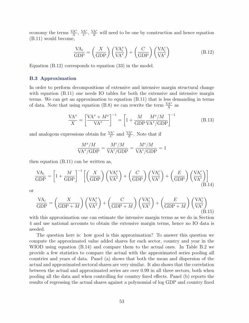
economy the terms VAx
X, VAc
C, VAe
Ewill need to be one by construction and hence equation
(B.11) would become,
VAi
GDP=
(X
GDP
)(VAx
i
VAx
)+
(C
GDP
)(VAc
i
VAc
)(B.12)
Equation (B.12) corresponds to equation (33) in the model.
B.3 Approximation
In order to perform decompositions of extensive and intensive margin structural changewith equation (B.11) one needs IO tables for both the extensive and intensive marginterms. We can get an approximation to equation (B.11) that is less demanding in termsof data. Note that using equation (B.8) we can rewrite the term VAx
Xas
VAx
X=
[VAx +Mx
VAx
]−1
=
[1 +
M
GDP
Mx/M
VAx/GDP
]−1
(B.13)
and analogous expressions obtain for VAc
Cand VAe
E. Note that if
Mx/M
VAx/GDP=
M c/M
VAc/GDP=
M e/M
VAe/GDP= 1
then equation (B.11) can be written as,
VAi
GDP=
[1 +
M
GDP
]−1 [(X
GDP
)(VAx
i
VAx
)+
(C
GDP
)(VAc
i
VAc
)+
(E
GDP
)(VAe
i
VAe
)](B.14)
or
VAi
GDP=
(X
GDP +M
)(VAx
i
VAx
)+
(C
GDP +M
)(VAc
i
VAc
)+
(E
GDP +M
)(VAe
i
VAe
)(B.15)
with this approximation one can estimate the intensive margin terms as we do in Section4 and use national accounts to obtain the extensive margin terms, hence no IO data isneeded.
The question here is: how good is this approximation? To answer this question wecompute the approximated value added shares for each sector, country and year in theWIOD using equation (B.14) and compare them to the actual ones. In Table B.2 weprovide a few statistics to compare the actual with the approximated series pooling allcountries and years of data. Panel (a) shows that both the mean and dispersion of theactual and approximated sectoral shares are very similar. It also shows that the correlationbetween the actual and approximated series are over 0.99 in all three sectors, both whenpooling all the data and when controlling for country fixed effects. Panel (b) reports theresults of regressing the actual shares against a polynomial of log GDP and country fixed
53
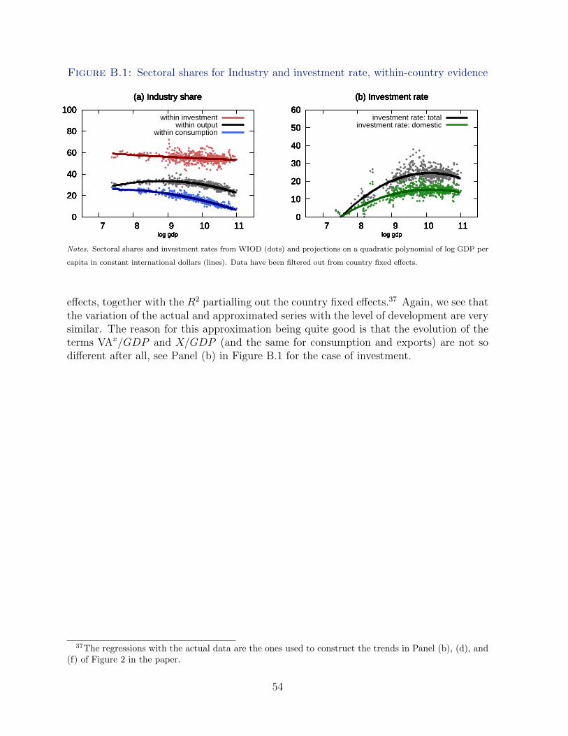
Figure B.1: Sectoral shares for Industry and investment rate, within-country evidence
0
20
40
60
80
100
7 8 9 10 11log gdp
(a) Industry share
within investmentwithin output
within consumption
0
20
40
60
80
100
7 8 9 10 11log gdp
(a) Industry share
0
20
40
60
80
100
7 8 9 10 11log gdp
(a) Industry share
0
20
40
60
80
100
7 8 9 10 11log gdp
(a) Industry share
0
20
40
60
80
100
7 8 9 10 11log gdp
(a) Industry share
0
20
40
60
80
100
7 8 9 10 11log gdp
(a) Industry share
0
20
40
60
80
100
7 8 9 10 11log gdp
(a) Industry share
0
10
20
30
40
50
60
7 8 9 10 11log gdp
(b) Investment rate
investment rate: totalinvestment rate: domestic
0
10
20
30
40
50
60
7 8 9 10 11log gdp
(b) Investment rate
0
10
20
30
40
50
60
7 8 9 10 11log gdp
(b) Investment rate
0
10
20
30
40
50
60
7 8 9 10 11log gdp
(b) Investment rate
0
10
20
30
40
50
60
7 8 9 10 11log gdp
(b) Investment rate
0
10
20
30
40
50
60
7 8 9 10 11log gdp
(b) Investment rate
Notes. Sectoral shares and investment rates from WIOD (dots) and projections on a quadratic polynomial of log GDP per
capita in constant international dollars (lines). Data have been filtered out from country fixed effects.
effects, together with the R2 partialling out the country fixed effects.37 Again, we see thatthe variation of the actual and approximated series with the level of development are verysimilar. The reason for this approximation being quite good is that the evolution of theterms VAx/GDP and X/GDP (and the same for consumption and exports) are not sodifferent after all, see Panel (b) in Figure B.1 for the case of investment.
37The regressions with the actual data are the ones used to construct the trends in Panel (b), (d), and(f) of Figure 2 in the paper.
54
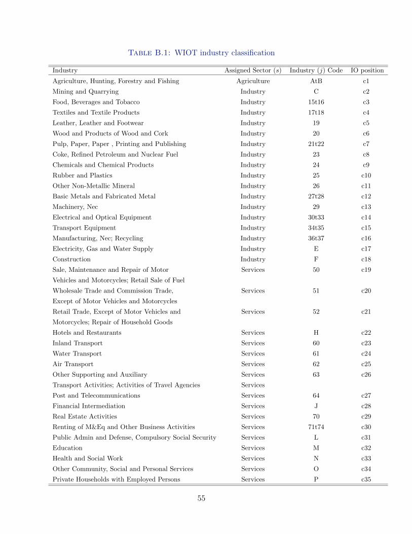
Table B.1: WIOT industry classification
Industry Assigned Sector (s) Industry (j) Code IO position
Agriculture, Hunting, Forestry and Fishing Agriculture AtB c1
Mining and Quarrying Industry C c2
Food, Beverages and Tobacco Industry 15t16 c3
Textiles and Textile Products Industry 17t18 c4
Leather, Leather and Footwear Industry 19 c5
Wood and Products of Wood and Cork Industry 20 c6
Pulp, Paper, Paper , Printing and Publishing Industry 21t22 c7
Coke, Refined Petroleum and Nuclear Fuel Industry 23 c8
Chemicals and Chemical Products Industry 24 c9
Rubber and Plastics Industry 25 c10
Other Non-Metallic Mineral Industry 26 c11
Basic Metals and Fabricated Metal Industry 27t28 c12
Machinery, Nec Industry 29 c13
Electrical and Optical Equipment Industry 30t33 c14
Transport Equipment Industry 34t35 c15
Manufacturing, Nec; Recycling Industry 36t37 c16
Electricity, Gas and Water Supply Industry E c17
Construction Industry F c18
Sale, Maintenance and Repair of Motor Services 50 c19
Vehicles and Motorcycles; Retail Sale of Fuel
Wholesale Trade and Commission Trade, Services 51 c20
Except of Motor Vehicles and Motorcycles
Retail Trade, Except of Motor Vehicles and Services 52 c21
Motorcycles; Repair of Household Goods
Hotels and Restaurants Services H c22
Inland Transport Services 60 c23
Water Transport Services 61 c24
Air Transport Services 62 c25
Other Supporting and Auxiliary Services 63 c26
Transport Activities; Activities of Travel Agencies Services
Post and Telecommunications Services 64 c27
Financial Intermediation Services J c28
Real Estate Activities Services 70 c29
Renting of M&Eq and Other Business Activities Services 71t74 c30
Public Admin and Defense, Compulsory Social Security Services L c31
Education Services M c32
Health and Social Work Services N c33
Other Community, Social and Personal Services Services O c34
Private Households with Employed Persons Services P c35
55
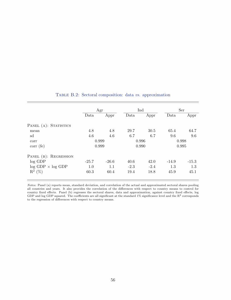
Table B.2: Sectoral composition: data vs. approximation
Agr Ind SerData Appr Data Appr Data Appr
Panel (a): Statisticsmean 4.8 4.8 29.7 30.5 65.4 64.7sd 4.6 4.6 6.7 6.7 9.6 9.6corr 0.999 0.996 0.998corr (fe) 0.999 0.990 0.995
Panel (b): Regressionlog GDP -25.7 -26.6 40.6 42.0 -14.9 -15.3log GDP × log GDP 1.0 1.1 -2.3 -2.4 1.3 1.3R2 (%) 60.3 60.4 19.4 18.8 45.9 45.1
Notes: Panel (a) reports mean, standard deviation, and correlation of the actual and approximated sectoral shares poolingall countries and years. It also provides the correlation of the differences with respect to country means to control forcountry fixed effects. Panel (b) regresses the sectoral shares, data and approximation, against country fixed effects, logGDP and log GDP squared. The coefficients are all significant at the standard 1% significance level and the R2 correspondsto the regression of differences with respect to country means.
56
Appendix C: Evolution of the investment rate for early starters
The evolution of the investment rate with economic development can also be exploredby use of the historical data put together by Jorda, Schularick, and Taylor (2017), whichoffers time series data from 17 countries between 1870 and 2013.
In Figure C.1 we plot the time series of investment for 6 different countries: GreatBritain, the US, Austria, France, Germany and the Netherlands against the log of percapita GDP in PPP. We can clearly see a hump in series of investment of the last fourcountries, see Panels (c)-(f). However, the hump is less clear for Great Britain (Panel a)and the US (Panel b), which represented the technology frontier in the first third and thelast two thirds of the sample period.
Next, in Figure C.2 we pool the data of all countries and years and plot the within-country variation in investment rates and saving rates as constructed in Section 2 of themain text, see Panel (a) and (b) respectively. We observe the same type of hump-shapedprofile as in the data of the PWT, although without a clear fall at the end of the process.However, given the long time series dimension of these data, we may also want to filterout year fixed effects capturing events like World wars or ups and downs in internationaltrade. Hence, Panel (c) and (d) plot the within-country variation in investment rates andsaving rate when we filter our country and year fixed effects. The results show a sharperhump in the sense that the decline of the investment and saving rate at the latest stagesof development is more pronounced.
57
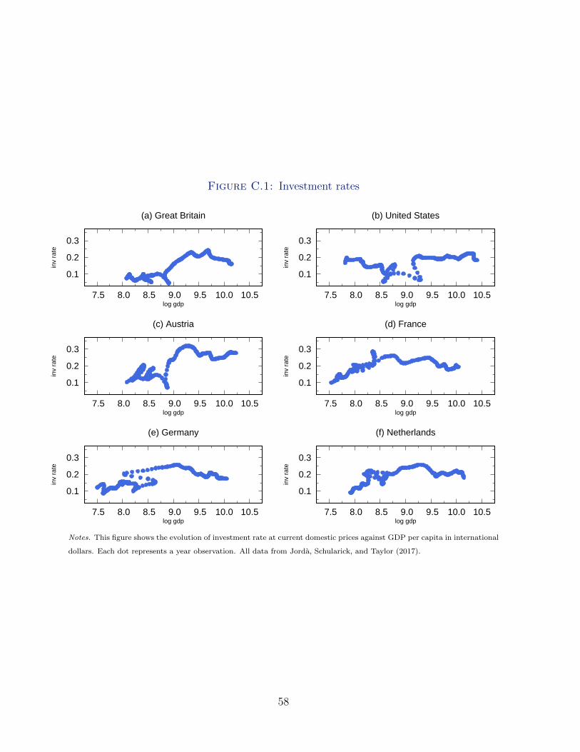
Figure C.1: Investment rates
0.1
0.2
0.3
7.5 8.0 8.5 9.0 9.5 10.0 10.5
inv
rate
log gdp
(a) Great Britain
0.1
0.2
0.3
7.5 8.0 8.5 9.0 9.5 10.0 10.5in
v ra
te
log gdp
(b) United States
0.1
0.2
0.3
7.5 8.0 8.5 9.0 9.5 10.0 10.5
inv
rate
log gdp
(c) Austria
0.1
0.2
0.3
7.5 8.0 8.5 9.0 9.5 10.0 10.5
inv
rate
log gdp
(d) France
0.1
0.2
0.3
7.5 8.0 8.5 9.0 9.5 10.0 10.5
inv
rate
log gdp
(e) Germany
0.1
0.2
0.3
7.5 8.0 8.5 9.0 9.5 10.0 10.5
inv
rate
log gdp
(f) Netherlands
Notes. This figure shows the evolution of investment rate at current domestic prices against GDP per capita in international
dollars. Each dot represents a year observation. All data from Jorda, Schularick, and Taylor (2017).
58
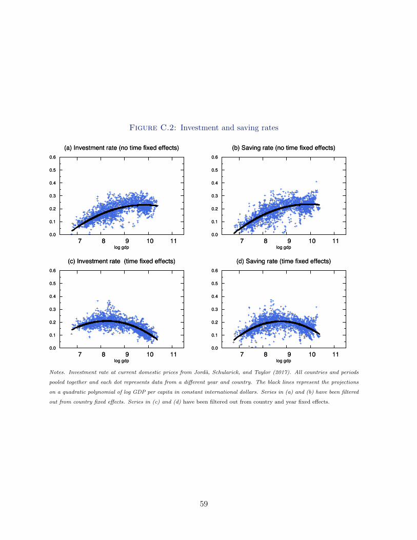
Figure C.2: Investment and saving rates
0.0
0.1
0.2
0.3
0.4
0.5
0.6
7 8 9 10 11log gdp
(a) Investment rate (no time fixed effects)
0.0
0.1
0.2
0.3
0.4
0.5
0.6
7 8 9 10 11log gdp
(a) Investment rate (no time fixed effects)
0.0
0.1
0.2
0.3
0.4
0.5
0.6
7 8 9 10 11log gdp
(b) Saving rate (no time fixed effects)
0.0
0.1
0.2
0.3
0.4
0.5
0.6
7 8 9 10 11log gdp
(b) Saving rate (no time fixed effects)
0.0
0.1
0.2
0.3
0.4
0.5
0.6
7 8 9 10 11log gdp
(c) Investment rate (time fixed effects)
0.0
0.1
0.2
0.3
0.4
0.5
0.6
7 8 9 10 11log gdp
(c) Investment rate (time fixed effects)
0.0
0.1
0.2
0.3
0.4
0.5
0.6
7 8 9 10 11log gdp
(d) Saving rate (time fixed effects)
0.0
0.1
0.2
0.3
0.4
0.5
0.6
7 8 9 10 11log gdp
(d) Saving rate (time fixed effects)
Notes. Investment rate at current domestic prices from Jorda, Schularick, and Taylor (2017). All countries and periods
pooled together and each dot represents data from a different year and country. The black lines represent the projections
on a quadratic polynomial of log GDP per capita in constant international dollars. Series in (a) and (b) have been filtered
out from country fixed effects. Series in (c) and (d) have been filtered out from country and year fixed effects.
59
Appendix D: Further model details
D.1 Characterization of the steady state
The BGP conditions imply that the habit stock is constant relative to the consumptionflow and given by,
h
c=
δhγ + δh
(where recall that (1 + γ) ≡ (1 + γB)(1 + γBc)). Then, the steady state capital k in themodel is characterized by the modified golden rule. That is, taking the Euler equation in(38) and imposing the BGP conditions we obtain,
(1 + γB) = β1/σ
[αχBx
[α + (1− α) k−ε
] 1−εε
+ (1− δk)]1/σ
(1 + γBc)1−σσ (D.1)
Then, output y in units of the investment good is given by the aggregate productionfunction in equation (31), which becomes
y = χBx
[αkε + (1− α)
]1/ε(D.2)
and the law of motion for capital
(1 + γB) = (1− δk) +y
k− c
k(D.3)
determines consumption c and investment x. Finally, from the interest rate equation (32)and the capital to labor ratio given by equation (41) we can get an expression for thecapital share,
rk
pxy= α
[α + (1− α) k−ε
]−1
(D.4)
Note that the whole path for the investment-specific technical change χtBxt matters inorder to determine the variables in BGP. This is because this path determines the BGPlevel χBx. For instance, what happens if the exogenous investment-specific technicalchange grows less than in our benchmark economy? The BGP value χ will be lower,meaning that the production of investment goods is more expensive in this counterfactualeconomy, which leads to a BGP with less capital, less investment, less output, and highercapital to output ratio, higher capital share and higher investment rate. To see this, notethat when χ is lower equation (D.1) implies that k is lower, equation (D.2) implies thatoutput y is lower, and equation (D.3) implies that investment x is lower. Also, equation
(41) shows that the capital to output ratio ky
is larger and equation (D.4) shows that the
60
capital share is larger. Finally, rewriting equation (D.3) as
(1 + γB) = (1− δk) +x
y
y
k
shows that the investment rate goes up. What is the logic of all this? The productionfunction is CES in capital and labor. A lower χ makes capital more expensive relative tolabor. This means that less capital is used in BGP (lower k), but with ES less than onemore is spent in capital, that is the capital share goes up. The lower capital level requiresa lower amount of investment to be sustained in the BGP and, because output falls morethan capital, both the capital to output and investment to output ratios increase. Whydoes output fall more than capital? Because it suffers the direct effect of the fall in χ andthe indirect effect of the fall in the capital stock.
D.2 BGP with Cobb-Douglas production functions
In the Cobb-Douglas case (ε = 0) the capital to output ratio is given by(pxtktyt
)−1
= χtBxt
(Bt
kt
)(1−α)
which is constant if capital kt grows at the rate γt given by
1 + γt = (1 + γBt) [(1 + γχt) (1 + γBxt)]1
1−α
Hence, it will be helpful to rewrite the model variables in units of the investment good
scaled by the productivity level Bt (χtBxt)1
1−α , which grows at the rate γt. Hence, let thehat variables be:
kt ≡ kt1
Bt (χtBxt)1
1−α
xt ≡ xt1
Bt (χtBxt)1
1−α
yt ≡ytpxt
1
Bt (χtBxt)1
1−α=
ytpct
1
BtBct (χtBxt)α
1−α
ct ≡pctctpxt
1
Bt (χtBxt)1
1−α= ct
1
BtBct (χtBxt)α
1−α
ht ≡pcthtpxt
1
Bt (χtBxt)1
1−α= ht
1
BtBct (χtBxt)α
1−α
61
Then, the production function in equation (31) becomes yt = kαt and the three differenceequations are:1− φ ht+1
ct+1
1− φ htct
ct+1
ct
σ
(1 + γt+1)σ = β[αkα−1
t+1 + (1− δk)] [1 + γBct+1
1 + γBxt+1
1
1 + γχt+1
]1−σ
(D.5)
kt+1
kt(1 + γt+1) = (1− δk) + kα−1
t − ct
kt+
1
Bt (χtBxt)α
1−α
∑i=a,m,s
ciBit
(D.6)
ht+1
ht(1 + γt+1) =
[(1− δh) + δh
ct
ht
] [1 + γBct+1
1 + γBxt+1
1
1 + γχt+1
]−1
(D.7)
In the Cobb-Douglas production case there is no role for Bt separately from the Bit,so without loss of generality we set γBt = 0 for all t. A BGP requires three things:
a) The rate of growth of the variables in units of the investment goods γt is constant(such that the left hand side of the three difference equations is constant)
b) The rate of growth of the relative productivity of investment and consumption(1 + γBct) / (1 + γBxt) (1 + γχt) is constant (in order to have the last term in equa-tions (D.5) and (D.7) constant)
c) The non-homotheticities play no role (in order to get the last term in equation (D.6)equal to zero)
Note that for condition (a) and (b) to be met simultaneously we need (1 + γBxt) (1 + γχt)and (1 + γBct) to be constant. Consider the case where γχt is constant. Then, conditions(a) and (b) require Bct and Bxt to grow at constant rates, which in general cannot happenbecause Bct and Bxt are time-changing weighted averages of the different Bit. Equations(28) and (27) clearly show that the two options for Bxt and Bct to grow at constant ratesare that either (i) ρx = 0 and ρc = 0 (unit elasticity of substitution within investment)and the sectoral productivities grow at constant but possibly different rates, or (ii) therate of growth of Bit are constant and equal in all sectors (symmetric productivity growthacross sectors). Of course, there is no structural change within investment goods in neithercase. Condition (c) will be met eventually because the last term in equation (D.6) vanishesasymptotically. When this happens, however, non-homothetic demands stop being a forceof sectoral reallocation. Hence, in the BGP output in units of the investment good, yt/pxt,investment xt, and consumption in units of the investment good pctct/pxt (see the law ofmotion for capital) grow all at the same rate γt, while the same variables in units of theconsumption good grow at the rate γt given by,
1 + γt = (1 + γBt) (1 + γBct) [(1 + γχt) (1 + γBxt)]α
1−α
D.3 A few particular cases
Our model specification nests a few well-known cases in the literature. In particular,setting ε = 0 and Bt = 1 ∀t to have a Cobb-Douglas production function and φ = 0 to
62
eliminate the habit stock:
Kongsamut, Rebelo, Xie. Assume that χt = 1, θxa = θxs = 0, cm = 0, ρc = 0, and thatBit grow all at the same rate γB. This is the Kongsamut, Rebelo, and Xie (2001) model,which assumes that there is no investment-specific technical change, that investment goodscome only from manufacturing, and that productivity growth is the same in all sectors.In this model structural change happens due to the non-homotheticities in demand. Byconstruction conditions (a) and (b) for BGP are met. Because the Bit all grow at thesame constant rate, condition (c) can only be met with structural change if
− cacs
=Ba0
Bs0
Then, the aggregate dynamics are given by the following system of two difference equa-tions,
ct+1
ct(1 + γB) = β
1σ
[α kα−1
t+1 + (1− δk)] 1σ
kt+1
kt(1 + γB) = (1− δk) + kα−1
t − ct
kt
which produce the same aggregate dynamics as the one-sector Ramsey model of growth.
Ngai, Pissarides. Assume that χt = 1, θxa = θxs = 0, and ci = 0 ∀i ∈ {a,m, s}.This is the Ngai and Pissarides (2007) model. As in Kongsamut, Rebelo, and Xie (2001)there is no investment specific technical change and investment goods are produced onlywith value added from manufacturing. Structural change is the result of asymmetricproductivity growth across sector and non-unit elasticity of substitution across goods.Condition (c) for BGP is met by construction. Condition (a) is met by assuming thatinvestment goods only come from manufacturing. To meet condition (b) the model needsto assume σ = 1. This gives again the same aggregate dynamics as in the one-sectorRamsey model of growth. The system of difference equations becomes:
ct+1
ct(1 + γBm) = β
[α kα−1
t+1 + (1− δk)]
kt+1
kt(1 + γBm) = (1− δk) + kα−1
t − ct
kt
Greenwood, Hercowitz, Krusell. Assume that θxi = θci and ci = 0 ∀i ∈ {a,m, s}.This implies that the investment and consumption goods are identical in terms of sectoralcomposition. If we further assume that Bit grow all at the same rate γBt there is no sectoralreallocation. This is the Greenwood, Hercowitz, and Krusell (1997) model (without capital
63
structures), whose aggregate dynamics are described by,
ct+1
ct[(1 + γχt) (1 + γBt)]
11−α = β
1σ
[α kα−1
t+1 + (1− δk)] 1σ
(1 + γχt)1−σσ
kt+1
kt[(1 + γχt) (1 + γBt)]
11−α = (1− δk) + kα−1
t − ct
kt
The model meets all required conditions for BGP whenever gammaχt and gammaBt areconstant.
Herrendorf, Rogerson, Valentinyi. Assume ci = 0, and σ = 1. This is the Her-rendorf, Rogerson, and Valentinyi (2018) model that allows for structural change withinconsumption and investment as ours but which differs in that there are no habits, thereare no income effects within consumption, and the utility is logarithmic. Then, condition(c) is met by construction, condition (b) is unneeded due to the log utility without habits,and for condition (a) to be satisfied they allow for time changing sectoral rates of growthsuch that (1 + γχt) (1 + γBxt) is constant. The aggregate dynamics are characterized bythe equations,
ct+1
ct[(1 + γχt) (1 + γBxt)]
11−α = β
[αkα−1
t+1 + (1− δk)]
kt+1
kt[(1 + γχt) (1 + γBxt)]
11−α = (1− δk) + kα−1
t − ct
kt
D.4 A two-good representation of the economy
This model economy can be rewritten as model with two final goods, investment andconsumption, whose production has hicks-neutral productivity χtBxt and Bct respectively.
Two-stage household problem. The household problem can be described as a twostage optimization process in which the household first solves the dynamic problem bychoosing the amount of spending in consumption pctct and investment pxtxt, and thensolves the static problem of choosing the composition of consumption and investment giventhe respective spendings. In this situation, the first stage is described by the followingLagrangian
∞∑t=0
βt
{u (ct − φht) + λt
[wt + rtkt −
(pctct −
∑i=a,m,s
pitci
)− pxtxt
]+ ηt
[(1− δk) kt + xt − kt+1
]}
that delivers the FOC for ct and xt described by equations (13) and (18) and the Eulerequation (11). Plugging equations (13) and (18) into (11) we get the Euler equation (22).In the second stage, at every period t the household maximizes the bundles of consumption
64
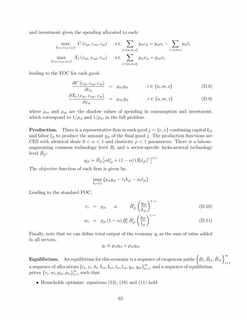
and investment given the spending allocated to each:
max{cat,cmt,cst}
C (cat, cmt, cst) s.t.∑
i={a,m,s}
pitcit = pctct −∑
i=a,m,s
pitci
max{xat,xmt,xst}
Xt (xat, xmt, xst) s.t.∑
i={a,m,s}
pitxit = pxtxt
leading to the FOC for each good:
∂C (cat, cmt, cst)
∂cit= µct pit i ∈ {a,m, s} (D.8)
∂Xt (xat, xmt, xst)
∂xit= µxt pit i ∈ {a,m, s} (D.9)
where µct and µxt are the shadow values of spending in consumption and investment,which correspond to 1/pct and 1/pxt in the full problem.
Production. There is a representative firm in each good j = {c, x} combining capital kjtand labor ljt to produce the amount yjt of the final good j. The production functions areCES with identical share 0 < α < 1 and elasticity ρ < 1 parameters. There is a labour-augmenting common technology level Bt and a sector-specific hicks-neutral technologylevel Bjt:
yjt = Bjt
[αkεjt + (1− α) (Btljt)
ε ]1/εThe objective function of each firm is given by,
maxkjt,ljt
{pjtyjt − rtkjt − wtljt}
Leading to the standard FOC,
rt = pjt α Bεjt
(yjtkjt
)1−ε
(D.10)
wt = pjt (1− α)Bεt B
εjt
(yjtljt
)1−ε
(D.11)
Finally, note that we can define total output of the economy yt as the sum of value addedin all sectors,
yt ≡ pctyct + pxtyxt
Equilibrium. An equilibrium for this economy is a sequence of exogenous paths{Bt, Bct, Bxt
}∞t=1
a sequence of allocations {ct, xt, kt, kct, kxt, lct, lxt, yct, yxt}∞t=1, and a sequence of equilibriumprices {rt, wt, pxt, pct}∞t=1 such that
• Households optimize: equations (13), (18) and (11) hold
65

• Firms optimize: equations (23), (24) hold
• All markets clear: kct + kxt = kt, lct + lxt = 1, yct = ct and yxt = xt
Note that in equilibrium the FOC of the firms imply that the capital to labor ratio is thesame for both goods and equal to the capital to labor ratio in the economy kct
lct= kxt
lxt= kt,
kt =
(α
1− αwtrtB−εt
) 11−ε
(D.12)
and that relative prices are given by
pxtpct
=Bct
Bxt
(D.13)
Hence, we can write total output and the interest rate in units of the investment good asa function of capital per capita in the economy,
yt/pxt = Bxt
[αkεt + (1− α)Bε
t
]1/ε(D.14)
rt/pxt = αBxt
(yt/pxtkt
)1−ε
(D.15)
Finally, we can characterize the equilibrium aggregate dynamics of this economy with thelaws of motion for ct and kt(ct+1 − φht+1
ct − φht
)σ= β
[Bct+1
Bct
Bxt
Bxt+1
][α Bxt+1
[α + (1− α)
(Bt+1
kt+1
)ε] 1−εε
+ (1− δk)
]kt+1
kt= (1− δk) + Bxt
[α + (1− α)
(Bt
kt
)ε]1/ε
− Bxt
Bct
ctkt
+
∑i=a,m,s
pitpxtci
kt
Analogy. Note that if we set Bct = Bct and Bxt = χtBxt the two economies are identical.
Appendix E: Creating the time series for the synthetic country
We have two panels of countries, WIOD and WDI-G10S-PWT, with data on several vari-ables of interest plus the GDP per capita in international dollars, yit. For the estimationof our model with these two panel data sets, we first want to create time series for asynthetic country that follows a stylized process of development extracted from these twopanel data sets. We proceed as follows.
1. Obtain the prediction functions for the variables of interest. Regress the desiredvariable zit on a low order polynomial of log yit and country fixed effects αzi:
zit = αzi + αz1 log yit + αz2 (log yit)2 + αz3 (log yit)
3 + εzit (E.1)
66
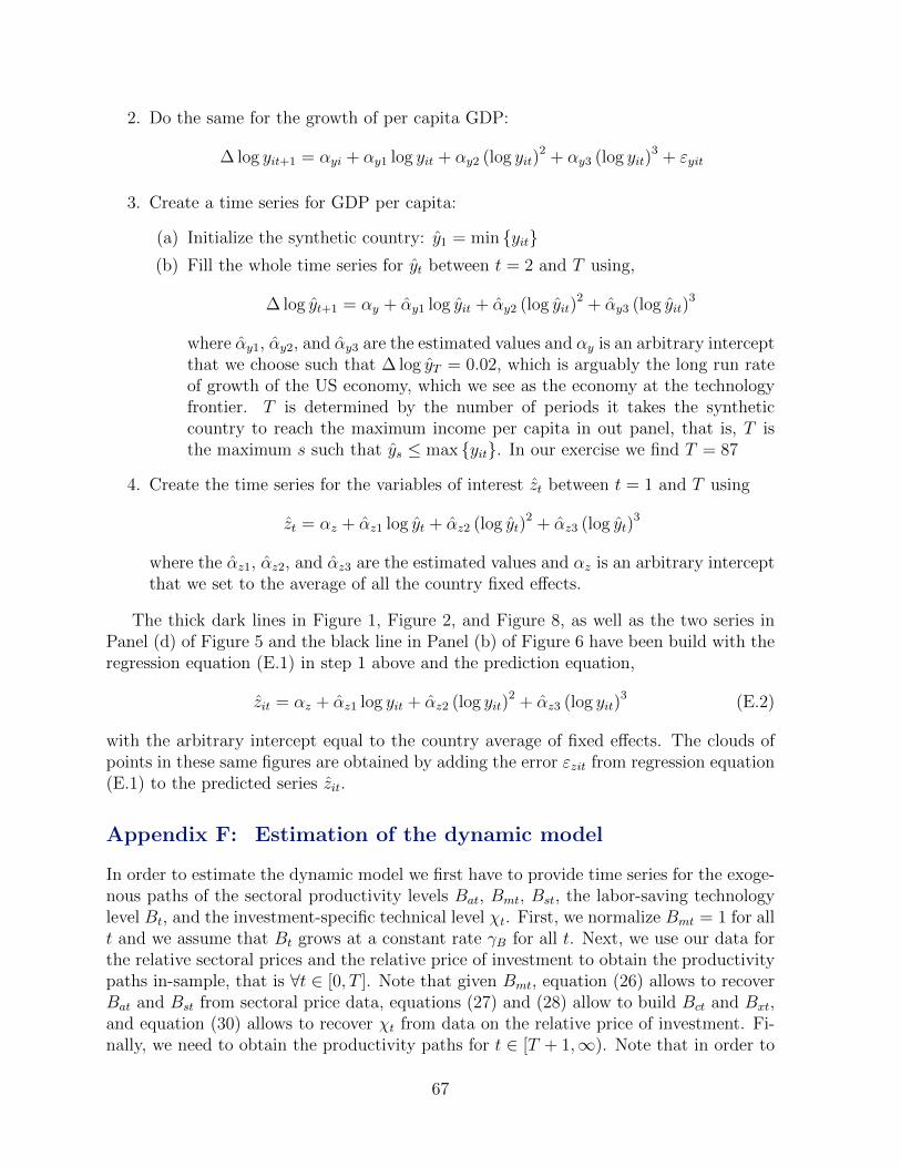
2. Do the same for the growth of per capita GDP:
∆ log yit+1 = αyi + αy1 log yit + αy2 (log yit)2 + αy3 (log yit)
3 + εyit
3. Create a time series for GDP per capita:
(a) Initialize the synthetic country: y1 = min {yit}(b) Fill the whole time series for yt between t = 2 and T using,
∆ log yt+1 = αy + αy1 log yit + αy2 (log yit)2 + αy3 (log yit)
3
where αy1, αy2, and αy3 are the estimated values and αy is an arbitrary interceptthat we choose such that ∆ log yT = 0.02, which is arguably the long run rateof growth of the US economy, which we see as the economy at the technologyfrontier. T is determined by the number of periods it takes the syntheticcountry to reach the maximum income per capita in out panel, that is, T isthe maximum s such that ys ≤ max {yit}. In our exercise we find T = 87
4. Create the time series for the variables of interest zt between t = 1 and T using
zt = αz + αz1 log yt + αz2 (log yt)2 + αz3 (log yt)
3
where the αz1, αz2, and αz3 are the estimated values and αz is an arbitrary interceptthat we set to the average of all the country fixed effects.
The thick dark lines in Figure 1, Figure 2, and Figure 8, as well as the two series inPanel (d) of Figure 5 and the black line in Panel (b) of Figure 6 have been build with theregression equation (E.1) in step 1 above and the prediction equation,
zit = αz + αz1 log yit + αz2 (log yit)2 + αz3 (log yit)
3 (E.2)
with the arbitrary intercept equal to the country average of fixed effects. The clouds ofpoints in these same figures are obtained by adding the error εzit from regression equation(E.1) to the predicted series zit.
Appendix F: Estimation of the dynamic model
In order to estimate the dynamic model we first have to provide time series for the exoge-nous paths of the sectoral productivity levels Bat, Bmt, Bst, the labor-saving technologylevel Bt, and the investment-specific technical level χt. First, we normalize Bmt = 1 for allt and we assume that Bt grows at a constant rate γB for all t. Next, we use our data forthe relative sectoral prices and the relative price of investment to obtain the productivitypaths in-sample, that is ∀t ∈ [0, T ]. Note that given Bmt, equation (26) allows to recoverBat and Bst from sectoral price data, equations (27) and (28) allow to build Bct and Bxt,and equation (30) allows to recover χt from data on the relative price of investment. Fi-nally, we need to obtain the productivity paths for t ∈ [T + 1,∞). Note that in order to
67

solve the model with a shooting algoritym we need a BGP at some point in the future.We set the exogenous paths of the different technology levels to be consistent with theBGP from T + 100 onwards, so we set set γχ = γBi = 0 ∀t ≥ T + 100 and we linearlyinterpolate the values of γBat, γBst, and γχt between T and T + 100.
For the estimation itself we implement the following procedure for a given ε:
1. Guess values for k0, h0, σ, φ, δh and γB
2. Obtain the level constant B0 to match output in the first period.
3. Steady state parameters. Choose α, β, and δk such that the BGP of the modeleconomy displays a capital share of 0.33, a capital to output ratio of 3, and aninvestment rate of 0.15, which in the model correspond to rk/y, pxk/y, and pxx/y.We proceed as follows. First, equation (D.3) in BGP can be written as,
(1 + γB) = (1− δk) +pxx
y
y
pxk
which pins down δk. Second, equation (D.1) can be rewritten as,
(1 + γB) = β1/σ
[(rk
y
)(pxk
y
)−1
+ (1− δk)
]1/σ
which pins down β. Finally, equation (D.4) for the capital share can written asfollows,
rk
y= α (χBx)
ε
(pxk
y
)εwhich determines α given the level constant χBx. The level constant χBx is itselfdetermined from the initial values of χt and Bxt at t = 0 and their subsequentgrowth until both χt and Bxt become constant at t = T +100. Note that the growthof χt and Bxt between t = 0 and t = T is determined by the growth of sectoralproductivities and the parameters of the demand system, two sets of objects thatare already determined.
4. Use a shooting algorithm to solve numerically for the whole transition between t = 0to the BGP and produce investment and output series between t = 0 and t = T .
5. Iterate on the vector of parameters k0, h0, σ, φ, δh and γB to minimize the sum ofsquared errors between the investment rate of the model and data and the averagerate of growth in the model and in the data
We iterate on this procedure trying different ε to obtain the best fit of the investmentrate between t = 0 and t = T .
68

Appendix G: Country by country estimation
G.1 Estimation details
We estimate equation (45) separately for each country, with all parameters being country-specific. We use the data from the combined WDI-G10S-PWT data set for each country asdescribed in Section 4.1 plus import and export rates from PWT. The function describingthe composition of exports piteit
petetis given by,
piteitpetet
= gei (Θei , t) + εeit
gei (Θei , t) ≡
exp (βei0 + βei1t)
1 + exp (βei0 + βei1t)
for sectors i ∈ {m, s}, while for sector i = a we can just write pateatpetet
= 1− pmtemtpetet
− pstestpetet
.To estimate the parameters of the demand system we turn to MCMC for compu-
tational reasons. First, by modelling the exports sectoral shares with an exponentialfunction we are increasing the nonlinearity of the model. The MCMC approach allows toreduce the dimensionality of the problem by splitting the estimation of the joint posteriordistribution of the parameters of the model in separate blocks with a Gibbs Samplingalgorithm. With non-linear estimations and large number of parameters this is a compu-tational advantage over the GMM or the quasi maximum likelihood, where one has to tosearch for all the parameters at the same time (Geweke 2005). Second, in a GMM esti-mator for the sectoral share of GDP there is nothing that restricts the estimated sectoralshares within consumption and within investment to lie between 0 and 1 for the entiretime series.38 Instead, the MCMC approach allows us to evaluate only combinations ofparameters that deliver predicted sectoral shares within goods that are bounded between0 and 1. And third, the MCMC is also particularly convenient for computing standarderrors in a set-up like the one we consider. For instance, if some of the sectoral shareswithin exports are close to zero, the inverse of the Jacobian of gei (Θe
i , t) will approachinfinity, which makes the calculation of standard errors in a GMM framework unfeasible.
We implement the MCMC as follows:
1. We start by estimating a model with ρ = 0 and with a linear version of the sectoralexport shares. Under these assumptions equation (45) becomes linear and we canestimate it with OLS.
2. Then, using the OLS estimates as initial values, we allow ρ to be different from 0and estimate the non-linear equation (45) but with still linear version of the sectoralexport shares within investment and within consumption using non-linear GMM.
38This is in contrast to the estimation of the synthetic country in Section 4.2 where we can exploita long time series input-output data from WIOD and estimate also equations (42) and (43) where thesectoral composition of consumption and investment are observed and bounded between 0 and 1.
69
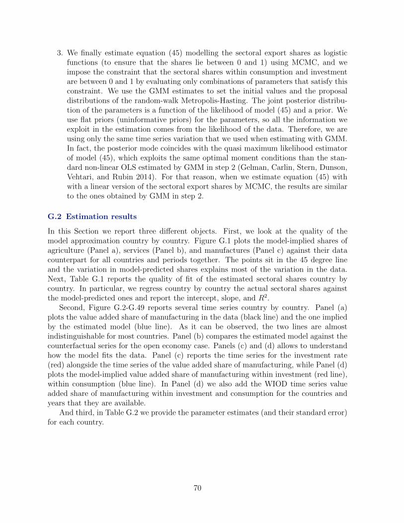
3. We finally estimate equation (45) modelling the sectoral export shares as logisticfunctions (to ensure that the shares lie between 0 and 1) using MCMC, and weimpose the constraint that the sectoral shares within consumption and investmentare between 0 and 1 by evaluating only combinations of parameters that satisfy thisconstraint. We use the GMM estimates to set the initial values and the proposaldistributions of the random-walk Metropolis-Hasting. The joint posterior distribu-tion of the parameters is a function of the likelihood of model (45) and a prior. Weuse flat priors (uninformative priors) for the parameters, so all the information weexploit in the estimation comes from the likelihood of the data. Therefore, we areusing only the same time series variation that we used when estimating with GMM.In fact, the posterior mode coincides with the quasi maximum likelihood estimatorof model (45), which exploits the same optimal moment conditions than the stan-dard non-linear OLS estimated by GMM in step 2 (Gelman, Carlin, Stern, Dunson,Vehtari, and Rubin 2014). For that reason, when we estimate equation (45) withwith a linear version of the sectoral export shares by MCMC, the results are similarto the ones obtained by GMM in step 2.
G.2 Estimation results
In this Section we report three different objects. First, we look at the quality of themodel approximation country by country. Figure G.1 plots the model-implied shares ofagriculture (Panel a), services (Panel b), and manufactures (Panel c) against their datacounterpart for all countries and periods together. The points sit in the 45 degree lineand the variation in model-predicted shares explains most of the variation in the data.Next, Table G.1 reports the quality of fit of the estimated sectoral shares country bycountry. In particular, we regress country by country the actual sectoral shares againstthe model-predicted ones and report the intercept, slope, and R2.
Second, Figure G.2-G.49 reports several time series country by country. Panel (a)plots the value added share of manufacturing in the data (black line) and the one impliedby the estimated model (blue line). As it can be observed, the two lines are almostindistinguishable for most countries. Panel (b) compares the estimated model against thecounterfactual series for the open economy case. Panels (c) and (d) allows to understandhow the model fits the data. Panel (c) reports the time series for the investment rate(red) alongside the time series of the value added share of manufacturing, while Panel (d)plots the model-implied value added share of manufacturing within investment (red line),within consumption (blue line). In Panel (d) we also add the WIOD time series valueadded share of manufacturing within investment and consumption for the countries andyears that they are available.
And third, in Table G.2 we provide the parameter estimates (and their standard error)for each country.
70
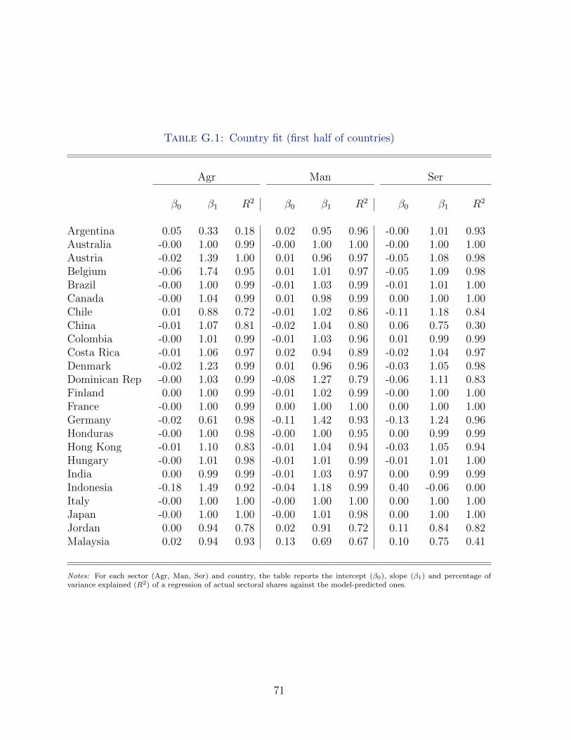
Table G.1: Country fit (first half of countries)
Agr Man Ser
β0 β1 R2 β0 β1 R2 β0 β1 R2
Argentina 0.05 0.33 0.18 0.02 0.95 0.96 -0.00 1.01 0.93Australia -0.00 1.00 0.99 -0.00 1.00 1.00 -0.00 1.00 1.00Austria -0.02 1.39 1.00 0.01 0.96 0.97 -0.05 1.08 0.98Belgium -0.06 1.74 0.95 0.01 1.01 0.97 -0.05 1.09 0.98Brazil -0.00 1.00 0.99 -0.01 1.03 0.99 -0.01 1.01 1.00Canada -0.00 1.04 0.99 0.01 0.98 0.99 0.00 1.00 1.00Chile 0.01 0.88 0.72 -0.01 1.02 0.86 -0.11 1.18 0.84China -0.01 1.07 0.81 -0.02 1.04 0.80 0.06 0.75 0.30Colombia -0.00 1.01 0.99 -0.01 1.03 0.96 0.01 0.99 0.99Costa Rica -0.01 1.06 0.97 0.02 0.94 0.89 -0.02 1.04 0.97Denmark -0.02 1.23 0.99 0.01 0.96 0.96 -0.03 1.05 0.98Dominican Rep -0.00 1.03 0.99 -0.08 1.27 0.79 -0.06 1.11 0.83Finland 0.00 1.00 0.99 -0.01 1.02 0.99 -0.00 1.00 1.00France -0.00 1.00 0.99 0.00 1.00 1.00 0.00 1.00 1.00Germany -0.02 0.61 0.98 -0.11 1.42 0.93 -0.13 1.24 0.96Honduras -0.00 1.00 0.98 -0.00 1.00 0.95 0.00 0.99 0.99Hong Kong -0.01 1.10 0.83 -0.01 1.04 0.94 -0.03 1.05 0.94Hungary -0.00 1.01 0.98 -0.01 1.01 0.99 -0.01 1.01 1.00India 0.00 0.99 0.99 -0.01 1.03 0.97 0.00 0.99 0.99Indonesia -0.18 1.49 0.92 -0.04 1.18 0.99 0.40 -0.06 0.00Italy -0.00 1.00 1.00 -0.00 1.00 1.00 0.00 1.00 1.00Japan -0.00 1.00 1.00 -0.00 1.01 0.98 0.00 1.00 1.00Jordan 0.00 0.94 0.78 0.02 0.91 0.72 0.11 0.84 0.82Malaysia 0.02 0.94 0.93 0.13 0.69 0.67 0.10 0.75 0.41
Notes: For each sector (Agr, Man, Ser) and country, the table reports the intercept (β0), slope (β1) and percentage ofvariance explained (R2) of a regression of actual sectoral shares against the model-predicted ones.
71
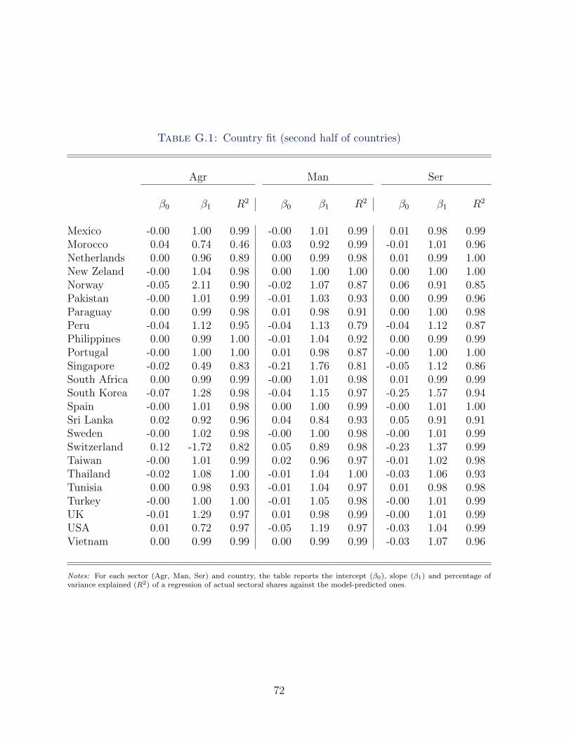
Table G.1: Country fit (second half of countries)
Agr Man Ser
β0 β1 R2 β0 β1 R2 β0 β1 R2
Mexico -0.00 1.00 0.99 -0.00 1.01 0.99 0.01 0.98 0.99Morocco 0.04 0.74 0.46 0.03 0.92 0.99 -0.01 1.01 0.96Netherlands 0.00 0.96 0.89 0.00 0.99 0.98 0.01 0.99 1.00New Zeland -0.00 1.04 0.98 0.00 1.00 1.00 0.00 1.00 1.00Norway -0.05 2.11 0.90 -0.02 1.07 0.87 0.06 0.91 0.85Pakistan -0.00 1.01 0.99 -0.01 1.03 0.93 0.00 0.99 0.96Paraguay 0.00 0.99 0.98 0.01 0.98 0.91 0.00 1.00 0.98Peru -0.04 1.12 0.95 -0.04 1.13 0.79 -0.04 1.12 0.87Philippines 0.00 0.99 1.00 -0.01 1.04 0.92 0.00 0.99 0.99Portugal -0.00 1.00 1.00 0.01 0.98 0.87 -0.00 1.00 1.00Singapore -0.02 0.49 0.83 -0.21 1.76 0.81 -0.05 1.12 0.86South Africa 0.00 0.99 0.99 -0.00 1.01 0.98 0.01 0.99 0.99South Korea -0.07 1.28 0.98 -0.04 1.15 0.97 -0.25 1.57 0.94Spain -0.00 1.01 0.98 0.00 1.00 0.99 -0.00 1.01 1.00Sri Lanka 0.02 0.92 0.96 0.04 0.84 0.93 0.05 0.91 0.91Sweden -0.00 1.02 0.98 -0.00 1.00 0.98 -0.00 1.01 0.99Switzerland 0.12 -1.72 0.82 0.05 0.89 0.98 -0.23 1.37 0.99Taiwan -0.00 1.01 0.99 0.02 0.96 0.97 -0.01 1.02 0.98Thailand -0.02 1.08 1.00 -0.01 1.04 1.00 -0.03 1.06 0.93Tunisia 0.00 0.98 0.93 -0.01 1.04 0.97 0.01 0.98 0.98Turkey -0.00 1.00 1.00 -0.01 1.05 0.98 -0.00 1.01 0.99UK -0.01 1.29 0.97 0.01 0.98 0.99 -0.00 1.01 0.99USA 0.01 0.72 0.97 -0.05 1.19 0.97 -0.03 1.04 0.99Vietnam 0.00 0.99 0.99 0.00 0.99 0.99 -0.03 1.07 0.96
Notes: For each sector (Agr, Man, Ser) and country, the table reports the intercept (β0), slope (β1) and percentage ofvariance explained (R2) of a regression of actual sectoral shares against the model-predicted ones.
72
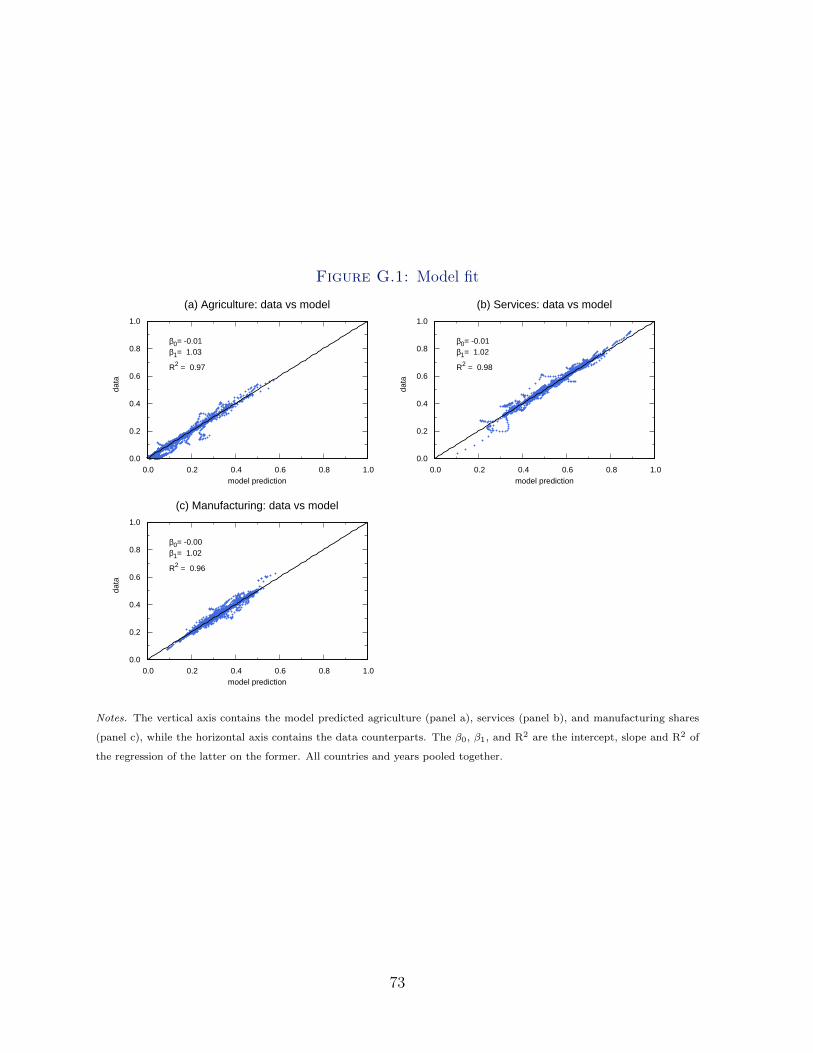
Figure G.1: Model fit
0.0
0.2
0.4
0.6
0.8
1.0
0.0 0.2 0.4 0.6 0.8 1.0
β0= -0.01β1= 1.03
R2 = 0.97
data
model prediction
(a) Agriculture: data vs model
0.0
0.2
0.4
0.6
0.8
1.0
0.0 0.2 0.4 0.6 0.8 1.0
β0= -0.01β1= 1.02
R2 = 0.98
data
model prediction
(b) Services: data vs model
0.0
0.2
0.4
0.6
0.8
1.0
0.0 0.2 0.4 0.6 0.8 1.0
β0= -0.00β1= 1.02
R2 = 0.96
data
model prediction
(c) Manufacturing: data vs model
Notes. The vertical axis contains the model predicted agriculture (panel a), services (panel b), and manufacturing shares
(panel c), while the horizontal axis contains the data counterparts. The β0, β1, and R2 are the intercept, slope and R2 of
the regression of the latter on the former. All countries and years pooled together.
73
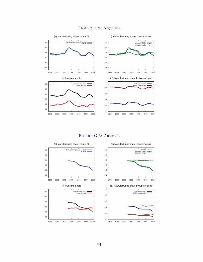
Figure G.2: Argentina
0.1
0.2
0.3
0.4
0.5
0.6
1950 1960 1970 1980 1990 2000 2010
(a) Manufacturing share: model fit
Manufacturing share: ArgentinaModel fit
0.1
0.2
0.3
0.4
0.5
0.6
1950 1960 1970 1980 1990 2000 2010
(b) Manufacturing share: counterfactual
Model fitIntensive margin
Extensive margin
0.1
0.2
0.3
0.4
0.5
0.6
1950 1960 1970 1980 1990 2000 2010
(c) Investment rate
Manufacturing shareInvestment rate
0.0
0.2
0.4
0.6
0.8
1.0
1950 1960 1970 1980 1990 2000 2010
(d) Manufacturing share by type of good
Within investmentWithin consumption
Figure G.3: Australia
0.1
0.2
0.3
0.4
0.5
0.6
1950 1960 1970 1980 1990 2000 2010
(a) Manufacturing share: model fit
Manufacturing share: AustraliaModel fit
0.1
0.2
0.3
0.4
0.5
0.6
1950 1960 1970 1980 1990 2000 2010
(b) Manufacturing share: counterfactual
Model fitIntensive margin
Extensive margin
0.1
0.2
0.3
0.4
0.5
0.6
1950 1960 1970 1980 1990 2000 2010
(c) Investment rate
Manufacturing shareInvestment rate
0.0
0.2
0.4
0.6
0.8
1.0
1950 1960 1970 1980 1990 2000 2010
(d) Manufacturing share by type of good
Within investmentWithin consumption
74

Figure G.4: Austria
0.1
0.2
0.3
0.4
0.5
0.6
1950 1960 1970 1980 1990 2000 2010
(a) Manufacturing share: model fit
Manufacturing share: AustriaModel fit
0.1
0.2
0.3
0.4
0.5
0.6
1950 1960 1970 1980 1990 2000 2010
(b) Manufacturing share: counterfactual
Model fitIntensive margin
Extensive margin
0.1
0.2
0.3
0.4
0.5
0.6
1950 1960 1970 1980 1990 2000 2010
(c) Investment rate
Manufacturing shareInvestment rate
0.0
0.2
0.4
0.6
0.8
1.0
1950 1960 1970 1980 1990 2000 2010
(d) Manufacturing share by type of good
Within investmentWithin consumption
Figure G.5: Belgium
0.1
0.2
0.3
0.4
0.5
0.6
1950 1960 1970 1980 1990 2000 2010
(a) Manufacturing share: model fit
Manufacturing share: BelgiumModel fit
0.1
0.2
0.3
0.4
0.5
0.6
1950 1960 1970 1980 1990 2000 2010
(b) Manufacturing share: counterfactual
Model fitIntensive margin
Extensive margin
0.1
0.2
0.3
0.4
0.5
0.6
1950 1960 1970 1980 1990 2000 2010
(c) Investment rate
Manufacturing shareInvestment rate
0.0
0.2
0.4
0.6
0.8
1.0
1950 1960 1970 1980 1990 2000 2010
(d) Manufacturing share by type of good
Within investmentWithin consumption
75
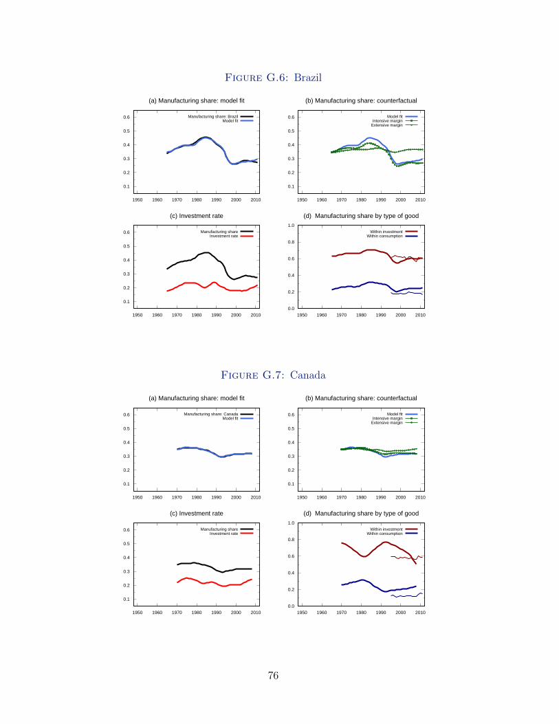
Figure G.6: Brazil
0.1
0.2
0.3
0.4
0.5
0.6
1950 1960 1970 1980 1990 2000 2010
(a) Manufacturing share: model fit
Manufacturing share: BrazilModel fit
0.1
0.2
0.3
0.4
0.5
0.6
1950 1960 1970 1980 1990 2000 2010
(b) Manufacturing share: counterfactual
Model fitIntensive margin
Extensive margin
0.1
0.2
0.3
0.4
0.5
0.6
1950 1960 1970 1980 1990 2000 2010
(c) Investment rate
Manufacturing shareInvestment rate
0.0
0.2
0.4
0.6
0.8
1.0
1950 1960 1970 1980 1990 2000 2010
(d) Manufacturing share by type of good
Within investmentWithin consumption
Figure G.7: Canada
0.1
0.2
0.3
0.4
0.5
0.6
1950 1960 1970 1980 1990 2000 2010
(a) Manufacturing share: model fit
Manufacturing share: CanadaModel fit
0.1
0.2
0.3
0.4
0.5
0.6
1950 1960 1970 1980 1990 2000 2010
(b) Manufacturing share: counterfactual
Model fitIntensive margin
Extensive margin
0.1
0.2
0.3
0.4
0.5
0.6
1950 1960 1970 1980 1990 2000 2010
(c) Investment rate
Manufacturing shareInvestment rate
0.0
0.2
0.4
0.6
0.8
1.0
1950 1960 1970 1980 1990 2000 2010
(d) Manufacturing share by type of good
Within investmentWithin consumption
76
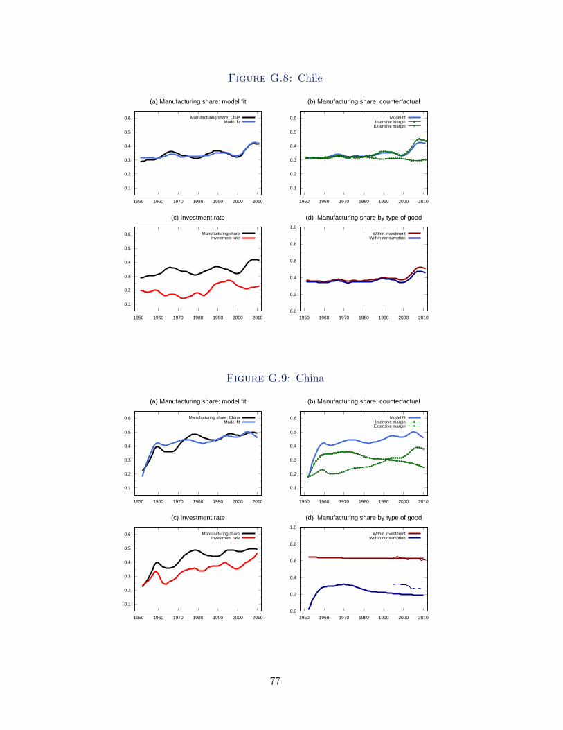
Figure G.8: Chile
0.1
0.2
0.3
0.4
0.5
0.6
1950 1960 1970 1980 1990 2000 2010
(a) Manufacturing share: model fit
Manufacturing share: ChileModel fit
0.1
0.2
0.3
0.4
0.5
0.6
1950 1960 1970 1980 1990 2000 2010
(b) Manufacturing share: counterfactual
Model fitIntensive margin
Extensive margin
0.1
0.2
0.3
0.4
0.5
0.6
1950 1960 1970 1980 1990 2000 2010
(c) Investment rate
Manufacturing shareInvestment rate
0.0
0.2
0.4
0.6
0.8
1.0
1950 1960 1970 1980 1990 2000 2010
(d) Manufacturing share by type of good
Within investmentWithin consumption
Figure G.9: China
0.1
0.2
0.3
0.4
0.5
0.6
1950 1960 1970 1980 1990 2000 2010
(a) Manufacturing share: model fit
Manufacturing share: ChinaModel fit
0.1
0.2
0.3
0.4
0.5
0.6
1950 1960 1970 1980 1990 2000 2010
(b) Manufacturing share: counterfactual
Model fitIntensive margin
Extensive margin
0.1
0.2
0.3
0.4
0.5
0.6
1950 1960 1970 1980 1990 2000 2010
(c) Investment rate
Manufacturing shareInvestment rate
0.0
0.2
0.4
0.6
0.8
1.0
1950 1960 1970 1980 1990 2000 2010
(d) Manufacturing share by type of good
Within investmentWithin consumption
77
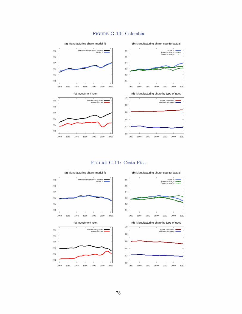
Figure G.10: Colombia
0.1
0.2
0.3
0.4
0.5
0.6
1950 1960 1970 1980 1990 2000 2010
(a) Manufacturing share: model fit
Manufacturing share: ColombiaModel fit
0.1
0.2
0.3
0.4
0.5
0.6
1950 1960 1970 1980 1990 2000 2010
(b) Manufacturing share: counterfactual
Model fitIntensive margin
Extensive margin
0.1
0.2
0.3
0.4
0.5
0.6
1950 1960 1970 1980 1990 2000 2010
(c) Investment rate
Manufacturing shareInvestment rate
0.0
0.2
0.4
0.6
0.8
1.0
1950 1960 1970 1980 1990 2000 2010
(d) Manufacturing share by type of good
Within investmentWithin consumption
Figure G.11: Costa Rica
0.1
0.2
0.3
0.4
0.5
0.6
1950 1960 1970 1980 1990 2000 2010
(a) Manufacturing share: model fit
Manufacturing share: CostaricaModel fit
0.1
0.2
0.3
0.4
0.5
0.6
1950 1960 1970 1980 1990 2000 2010
(b) Manufacturing share: counterfactual
Model fitIntensive margin
Extensive margin
0.1
0.2
0.3
0.4
0.5
0.6
1950 1960 1970 1980 1990 2000 2010
(c) Investment rate
Manufacturing shareInvestment rate
0.0
0.2
0.4
0.6
0.8
1.0
1950 1960 1970 1980 1990 2000 2010
(d) Manufacturing share by type of good
Within investmentWithin consumption
78

Figure G.12: Denmark
0.1
0.2
0.3
0.4
0.5
0.6
1950 1960 1970 1980 1990 2000 2010
(a) Manufacturing share: model fit
Manufacturing share: DenmarkModel fit
0.1
0.2
0.3
0.4
0.5
0.6
1950 1960 1970 1980 1990 2000 2010
(b) Manufacturing share: counterfactual
Model fitIntensive margin
Extensive margin
0.1
0.2
0.3
0.4
0.5
0.6
1950 1960 1970 1980 1990 2000 2010
(c) Investment rate
Manufacturing shareInvestment rate
0.0
0.2
0.4
0.6
0.8
1.0
1950 1960 1970 1980 1990 2000 2010
(d) Manufacturing share by type of good
Within investmentWithin consumption
Figure G.13: Dominican Republic
0.1
0.2
0.3
0.4
0.5
0.6
1950 1960 1970 1980 1990 2000 2010
(a) Manufacturing share: model fit
Manufacturing share: DominicanrepModel fit
0.1
0.2
0.3
0.4
0.5
0.6
1950 1960 1970 1980 1990 2000 2010
(b) Manufacturing share: counterfactual
Model fitIntensive margin
Extensive margin
0.1
0.2
0.3
0.4
0.5
0.6
1950 1960 1970 1980 1990 2000 2010
(c) Investment rate
Manufacturing shareInvestment rate
0.0
0.2
0.4
0.6
0.8
1.0
1950 1960 1970 1980 1990 2000 2010
(d) Manufacturing share by type of good
Within investmentWithin consumption
79

Figure G.14: Finland
0.1
0.2
0.3
0.4
0.5
0.6
1950 1960 1970 1980 1990 2000 2010
(a) Manufacturing share: model fit
Manufacturing share: FinlandModel fit
0.1
0.2
0.3
0.4
0.5
0.6
1950 1960 1970 1980 1990 2000 2010
(b) Manufacturing share: counterfactual
Model fitIntensive margin
Extensive margin
0.1
0.2
0.3
0.4
0.5
0.6
1950 1960 1970 1980 1990 2000 2010
(c) Investment rate
Manufacturing shareInvestment rate
0.0
0.2
0.4
0.6
0.8
1.0
1950 1960 1970 1980 1990 2000 2010
(d) Manufacturing share by type of good
Within investmentWithin consumption
Figure G.15: France
0.1
0.2
0.3
0.4
0.5
0.6
1950 1960 1970 1980 1990 2000 2010
(a) Manufacturing share: model fit
Manufacturing share: FranceModel fit
0.1
0.2
0.3
0.4
0.5
0.6
1950 1960 1970 1980 1990 2000 2010
(b) Manufacturing share: counterfactual
Model fitIntensive margin
Extensive margin
0.1
0.2
0.3
0.4
0.5
0.6
1950 1960 1970 1980 1990 2000 2010
(c) Investment rate
Manufacturing shareInvestment rate
0.0
0.2
0.4
0.6
0.8
1.0
1950 1960 1970 1980 1990 2000 2010
(d) Manufacturing share by type of good
Within investmentWithin consumption
80
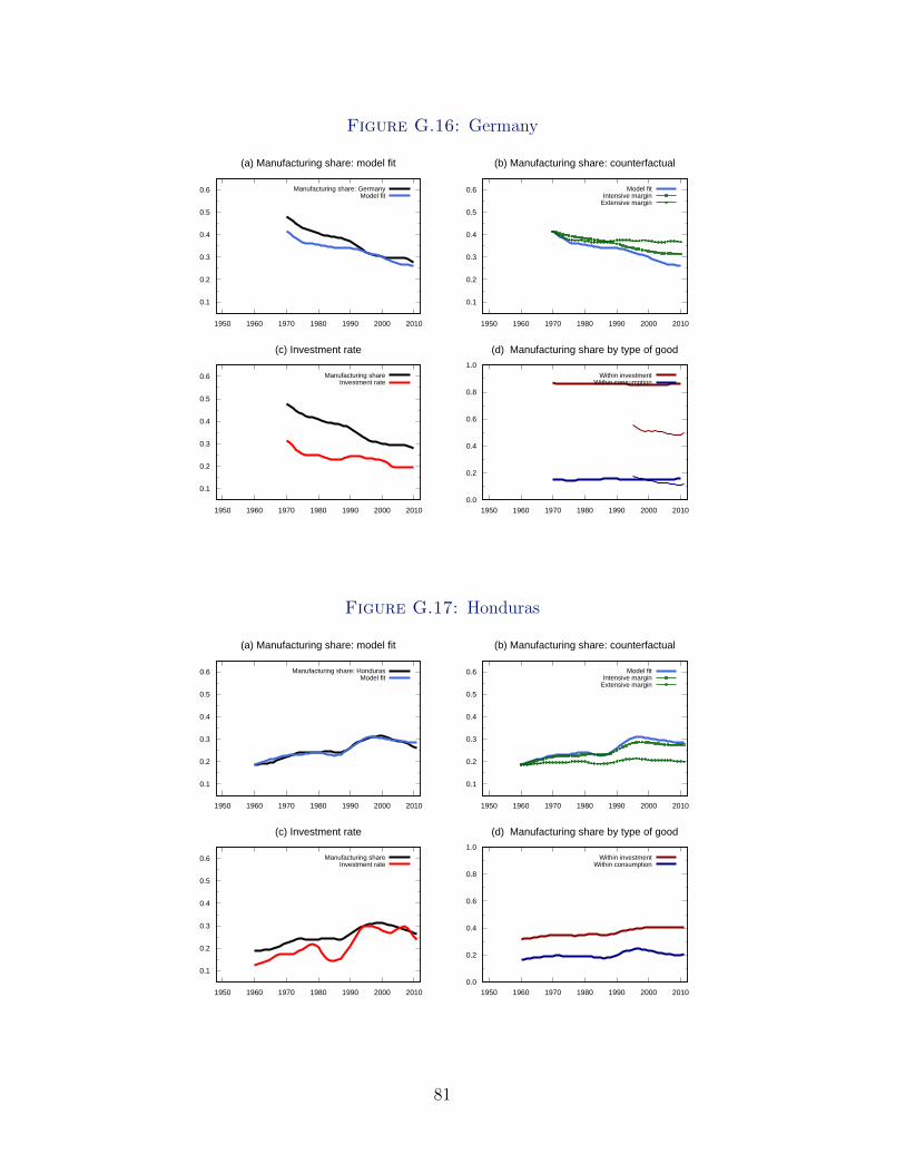
Figure G.16: Germany
0.1
0.2
0.3
0.4
0.5
0.6
1950 1960 1970 1980 1990 2000 2010
(a) Manufacturing share: model fit
Manufacturing share: GermanyModel fit
0.1
0.2
0.3
0.4
0.5
0.6
1950 1960 1970 1980 1990 2000 2010
(b) Manufacturing share: counterfactual
Model fitIntensive margin
Extensive margin
0.1
0.2
0.3
0.4
0.5
0.6
1950 1960 1970 1980 1990 2000 2010
(c) Investment rate
Manufacturing shareInvestment rate
0.0
0.2
0.4
0.6
0.8
1.0
1950 1960 1970 1980 1990 2000 2010
(d) Manufacturing share by type of good
Within investmentWithin consumption
Figure G.17: Honduras
0.1
0.2
0.3
0.4
0.5
0.6
1950 1960 1970 1980 1990 2000 2010
(a) Manufacturing share: model fit
Manufacturing share: HondurasModel fit
0.1
0.2
0.3
0.4
0.5
0.6
1950 1960 1970 1980 1990 2000 2010
(b) Manufacturing share: counterfactual
Model fitIntensive margin
Extensive margin
0.1
0.2
0.3
0.4
0.5
0.6
1950 1960 1970 1980 1990 2000 2010
(c) Investment rate
Manufacturing shareInvestment rate
0.0
0.2
0.4
0.6
0.8
1.0
1950 1960 1970 1980 1990 2000 2010
(d) Manufacturing share by type of good
Within investmentWithin consumption
81
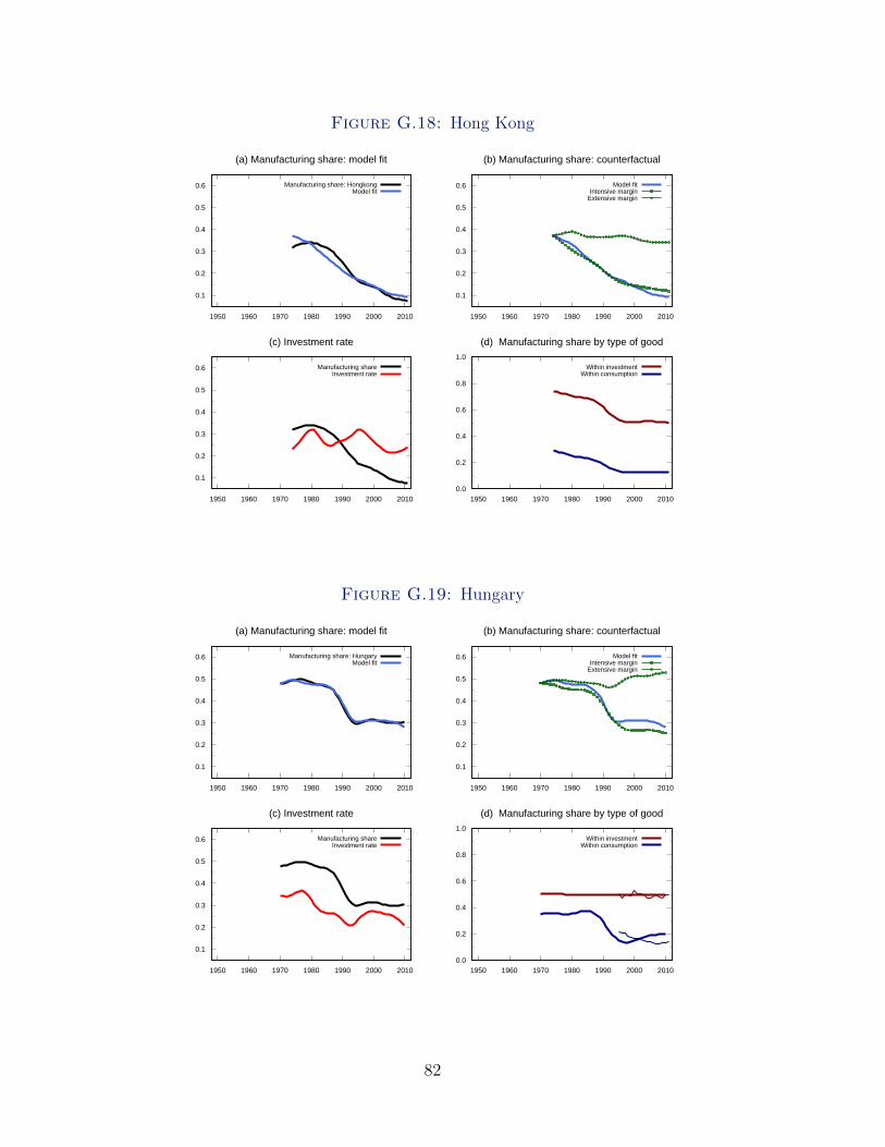
Figure G.18: Hong Kong
0.1
0.2
0.3
0.4
0.5
0.6
1950 1960 1970 1980 1990 2000 2010
(a) Manufacturing share: model fit
Manufacturing share: HongkongModel fit
0.1
0.2
0.3
0.4
0.5
0.6
1950 1960 1970 1980 1990 2000 2010
(b) Manufacturing share: counterfactual
Model fitIntensive margin
Extensive margin
0.1
0.2
0.3
0.4
0.5
0.6
1950 1960 1970 1980 1990 2000 2010
(c) Investment rate
Manufacturing shareInvestment rate
0.0
0.2
0.4
0.6
0.8
1.0
1950 1960 1970 1980 1990 2000 2010
(d) Manufacturing share by type of good
Within investmentWithin consumption
Figure G.19: Hungary
0.1
0.2
0.3
0.4
0.5
0.6
1950 1960 1970 1980 1990 2000 2010
(a) Manufacturing share: model fit
Manufacturing share: HungaryModel fit
0.1
0.2
0.3
0.4
0.5
0.6
1950 1960 1970 1980 1990 2000 2010
(b) Manufacturing share: counterfactual
Model fitIntensive margin
Extensive margin
0.1
0.2
0.3
0.4
0.5
0.6
1950 1960 1970 1980 1990 2000 2010
(c) Investment rate
Manufacturing shareInvestment rate
0.0
0.2
0.4
0.6
0.8
1.0
1950 1960 1970 1980 1990 2000 2010
(d) Manufacturing share by type of good
Within investmentWithin consumption
82
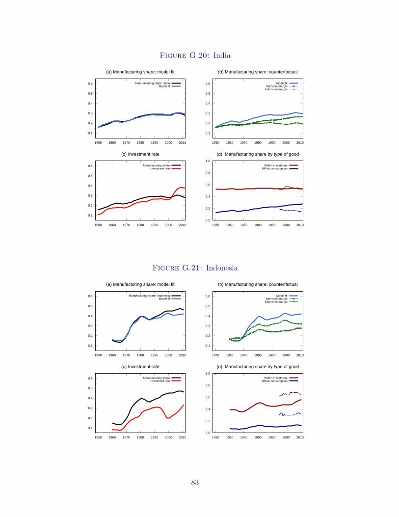
Figure G.20: India
0.1
0.2
0.3
0.4
0.5
0.6
1950 1960 1970 1980 1990 2000 2010
(a) Manufacturing share: model fit
Manufacturing share: IndiaModel fit
0.1
0.2
0.3
0.4
0.5
0.6
1950 1960 1970 1980 1990 2000 2010
(b) Manufacturing share: counterfactual
Model fitIntensive margin
Extensive margin
0.1
0.2
0.3
0.4
0.5
0.6
1950 1960 1970 1980 1990 2000 2010
(c) Investment rate
Manufacturing shareInvestment rate
0.0
0.2
0.4
0.6
0.8
1.0
1950 1960 1970 1980 1990 2000 2010
(d) Manufacturing share by type of good
Within investmentWithin consumption
Figure G.21: Indonesia
0.1
0.2
0.3
0.4
0.5
0.6
1950 1960 1970 1980 1990 2000 2010
(a) Manufacturing share: model fit
Manufacturing share: IndonesiaModel fit
0.1
0.2
0.3
0.4
0.5
0.6
1950 1960 1970 1980 1990 2000 2010
(b) Manufacturing share: counterfactual
Model fitIntensive margin
Extensive margin
0.1
0.2
0.3
0.4
0.5
0.6
1950 1960 1970 1980 1990 2000 2010
(c) Investment rate
Manufacturing shareInvestment rate
0.0
0.2
0.4
0.6
0.8
1.0
1950 1960 1970 1980 1990 2000 2010
(d) Manufacturing share by type of good
Within investmentWithin consumption
83

Figure G.22: Italy
0.1
0.2
0.3
0.4
0.5
0.6
1950 1960 1970 1980 1990 2000 2010
(a) Manufacturing share: model fit
Manufacturing share: ItalyModel fit
0.1
0.2
0.3
0.4
0.5
0.6
1950 1960 1970 1980 1990 2000 2010
(b) Manufacturing share: counterfactual
Model fitIntensive margin
Extensive margin
0.1
0.2
0.3
0.4
0.5
0.6
1950 1960 1970 1980 1990 2000 2010
(c) Investment rate
Manufacturing shareInvestment rate
0.0
0.2
0.4
0.6
0.8
1.0
1950 1960 1970 1980 1990 2000 2010
(d) Manufacturing share by type of good
Within investmentWithin consumption
Figure G.23: Japan
0.1
0.2
0.3
0.4
0.5
0.6
1950 1960 1970 1980 1990 2000 2010
(a) Manufacturing share: model fit
Manufacturing share: JapanModel fit
0.1
0.2
0.3
0.4
0.5
0.6
1950 1960 1970 1980 1990 2000 2010
(b) Manufacturing share: counterfactual
Model fitIntensive margin
Extensive margin
0.1
0.2
0.3
0.4
0.5
0.6
1950 1960 1970 1980 1990 2000 2010
(c) Investment rate
Manufacturing shareInvestment rate
0.0
0.2
0.4
0.6
0.8
1.0
1950 1960 1970 1980 1990 2000 2010
(d) Manufacturing share by type of good
Within investmentWithin consumption
84
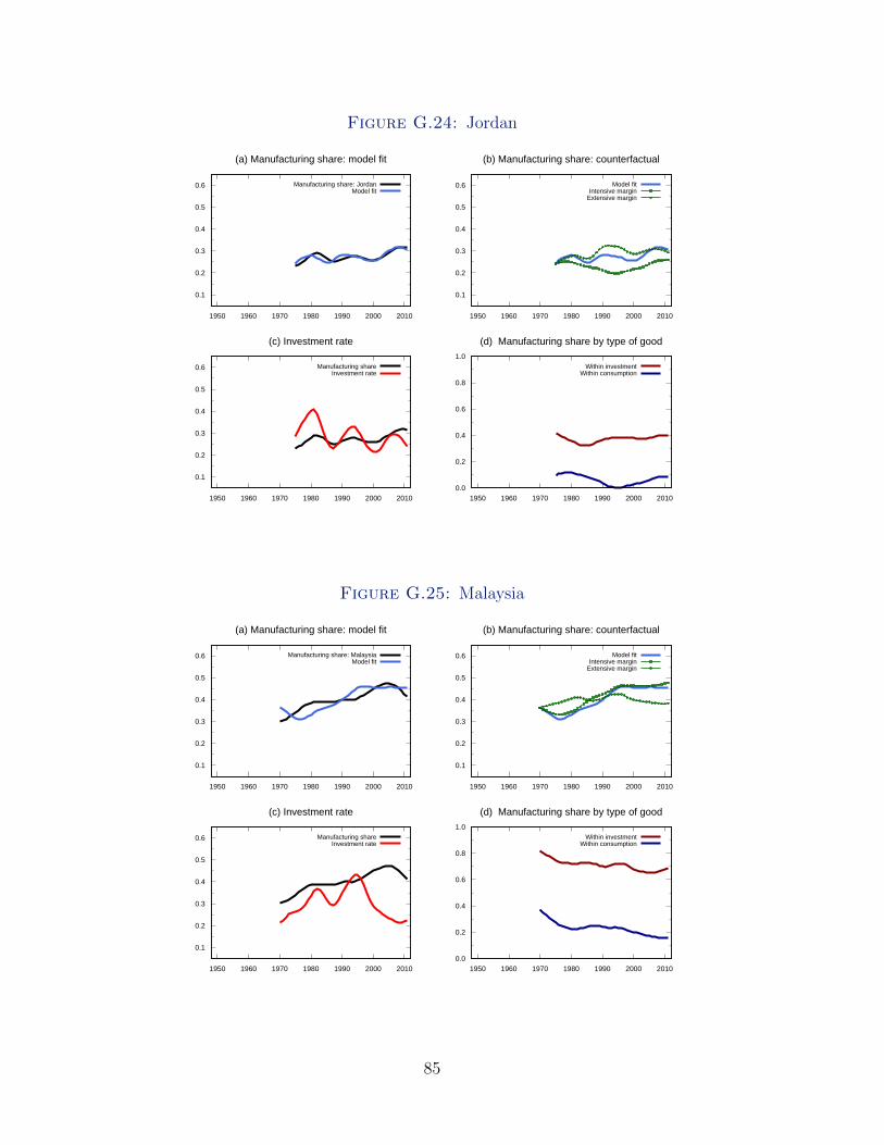
Figure G.24: Jordan
0.1
0.2
0.3
0.4
0.5
0.6
1950 1960 1970 1980 1990 2000 2010
(a) Manufacturing share: model fit
Manufacturing share: JordanModel fit
0.1
0.2
0.3
0.4
0.5
0.6
1950 1960 1970 1980 1990 2000 2010
(b) Manufacturing share: counterfactual
Model fitIntensive margin
Extensive margin
0.1
0.2
0.3
0.4
0.5
0.6
1950 1960 1970 1980 1990 2000 2010
(c) Investment rate
Manufacturing shareInvestment rate
0.0
0.2
0.4
0.6
0.8
1.0
1950 1960 1970 1980 1990 2000 2010
(d) Manufacturing share by type of good
Within investmentWithin consumption
Figure G.25: Malaysia
0.1
0.2
0.3
0.4
0.5
0.6
1950 1960 1970 1980 1990 2000 2010
(a) Manufacturing share: model fit
Manufacturing share: MalaysiaModel fit
0.1
0.2
0.3
0.4
0.5
0.6
1950 1960 1970 1980 1990 2000 2010
(b) Manufacturing share: counterfactual
Model fitIntensive margin
Extensive margin
0.1
0.2
0.3
0.4
0.5
0.6
1950 1960 1970 1980 1990 2000 2010
(c) Investment rate
Manufacturing shareInvestment rate
0.0
0.2
0.4
0.6
0.8
1.0
1950 1960 1970 1980 1990 2000 2010
(d) Manufacturing share by type of good
Within investmentWithin consumption
85
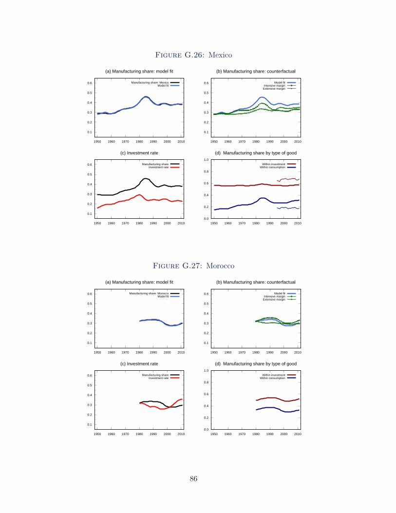
Figure G.26: Mexico
0.1
0.2
0.3
0.4
0.5
0.6
1950 1960 1970 1980 1990 2000 2010
(a) Manufacturing share: model fit
Manufacturing share: MexicoModel fit
0.1
0.2
0.3
0.4
0.5
0.6
1950 1960 1970 1980 1990 2000 2010
(b) Manufacturing share: counterfactual
Model fitIntensive margin
Extensive margin
0.1
0.2
0.3
0.4
0.5
0.6
1950 1960 1970 1980 1990 2000 2010
(c) Investment rate
Manufacturing shareInvestment rate
0.0
0.2
0.4
0.6
0.8
1.0
1950 1960 1970 1980 1990 2000 2010
(d) Manufacturing share by type of good
Within investmentWithin consumption
Figure G.27: Morocco
0.1
0.2
0.3
0.4
0.5
0.6
1950 1960 1970 1980 1990 2000 2010
(a) Manufacturing share: model fit
Manufacturing share: MoroccoModel fit
0.1
0.2
0.3
0.4
0.5
0.6
1950 1960 1970 1980 1990 2000 2010
(b) Manufacturing share: counterfactual
Model fitIntensive margin
Extensive margin
0.1
0.2
0.3
0.4
0.5
0.6
1950 1960 1970 1980 1990 2000 2010
(c) Investment rate
Manufacturing shareInvestment rate
0.0
0.2
0.4
0.6
0.8
1.0
1950 1960 1970 1980 1990 2000 2010
(d) Manufacturing share by type of good
Within investmentWithin consumption
86
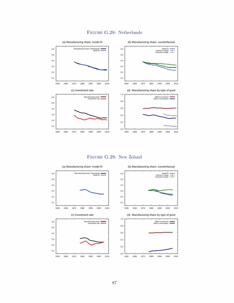
Figure G.28: Netherlands
0.1
0.2
0.3
0.4
0.5
0.6
1950 1960 1970 1980 1990 2000 2010
(a) Manufacturing share: model fit
Manufacturing share: NetherlandsModel fit
0.1
0.2
0.3
0.4
0.5
0.6
1950 1960 1970 1980 1990 2000 2010
(b) Manufacturing share: counterfactual
Model fitIntensive margin
Extensive margin
0.1
0.2
0.3
0.4
0.5
0.6
1950 1960 1970 1980 1990 2000 2010
(c) Investment rate
Manufacturing shareInvestment rate
0.0
0.2
0.4
0.6
0.8
1.0
1950 1960 1970 1980 1990 2000 2010
(d) Manufacturing share by type of good
Within investmentWithin consumption
Figure G.29: New Zeland
0.1
0.2
0.3
0.4
0.5
0.6
1950 1960 1970 1980 1990 2000 2010
(a) Manufacturing share: model fit
Manufacturing share: NewzelandModel fit
0.1
0.2
0.3
0.4
0.5
0.6
1950 1960 1970 1980 1990 2000 2010
(b) Manufacturing share: counterfactual
Model fitIntensive margin
Extensive margin
0.1
0.2
0.3
0.4
0.5
0.6
1950 1960 1970 1980 1990 2000 2010
(c) Investment rate
Manufacturing shareInvestment rate
0.0
0.2
0.4
0.6
0.8
1.0
1950 1960 1970 1980 1990 2000 2010
(d) Manufacturing share by type of good
Within investmentWithin consumption
87

Figure G.30: Norway
0.1
0.2
0.3
0.4
0.5
0.6
1950 1960 1970 1980 1990 2000 2010
(a) Manufacturing share: model fit
Manufacturing share: NorwayModel fit
0.1
0.2
0.3
0.4
0.5
0.6
1950 1960 1970 1980 1990 2000 2010
(b) Manufacturing share: counterfactual
Model fitIntensive margin
Extensive margin
0.1
0.2
0.3
0.4
0.5
0.6
1950 1960 1970 1980 1990 2000 2010
(c) Investment rate
Manufacturing shareInvestment rate
0.0
0.2
0.4
0.6
0.8
1.0
1950 1960 1970 1980 1990 2000 2010
(d) Manufacturing share by type of good
Within investmentWithin consumption
Figure G.31: Pakistan
0.1
0.2
0.3
0.4
0.5
0.6
1950 1960 1970 1980 1990 2000 2010
(a) Manufacturing share: model fit
Manufacturing share: PakistanModel fit
0.1
0.2
0.3
0.4
0.5
0.6
1950 1960 1970 1980 1990 2000 2010
(b) Manufacturing share: counterfactual
Model fitIntensive margin
Extensive margin
0.1
0.2
0.3
0.4
0.5
0.6
1950 1960 1970 1980 1990 2000 2010
(c) Investment rate
Manufacturing shareInvestment rate
0.0
0.2
0.4
0.6
0.8
1.0
1950 1960 1970 1980 1990 2000 2010
(d) Manufacturing share by type of good
Within investmentWithin consumption
88
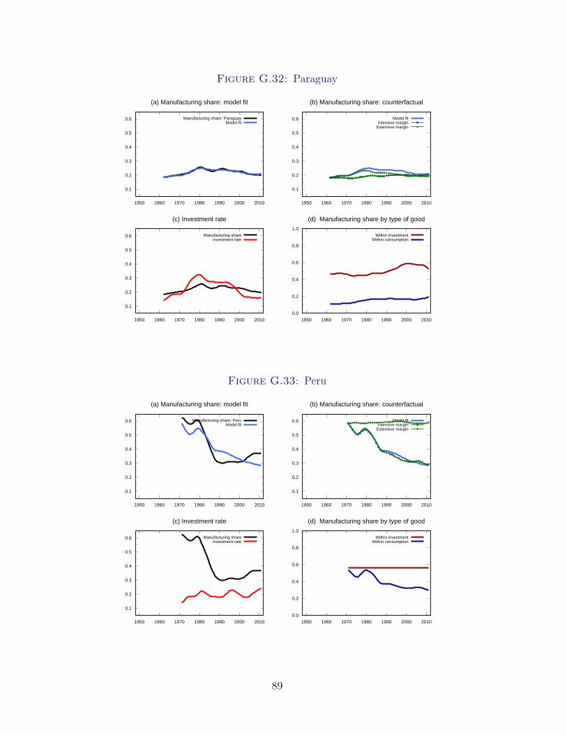
Figure G.32: Paraguay
0.1
0.2
0.3
0.4
0.5
0.6
1950 1960 1970 1980 1990 2000 2010
(a) Manufacturing share: model fit
Manufacturing share: ParaguayModel fit
0.1
0.2
0.3
0.4
0.5
0.6
1950 1960 1970 1980 1990 2000 2010
(b) Manufacturing share: counterfactual
Model fitIntensive margin
Extensive margin
0.1
0.2
0.3
0.4
0.5
0.6
1950 1960 1970 1980 1990 2000 2010
(c) Investment rate
Manufacturing shareInvestment rate
0.0
0.2
0.4
0.6
0.8
1.0
1950 1960 1970 1980 1990 2000 2010
(d) Manufacturing share by type of good
Within investmentWithin consumption
Figure G.33: Peru
0.1
0.2
0.3
0.4
0.5
0.6
1950 1960 1970 1980 1990 2000 2010
(a) Manufacturing share: model fit
Manufacturing share: PeruModel fit
0.1
0.2
0.3
0.4
0.5
0.6
1950 1960 1970 1980 1990 2000 2010
(b) Manufacturing share: counterfactual
Model fitIntensive margin
Extensive margin
0.1
0.2
0.3
0.4
0.5
0.6
1950 1960 1970 1980 1990 2000 2010
(c) Investment rate
Manufacturing shareInvestment rate
0.0
0.2
0.4
0.6
0.8
1.0
1950 1960 1970 1980 1990 2000 2010
(d) Manufacturing share by type of good
Within investmentWithin consumption
89
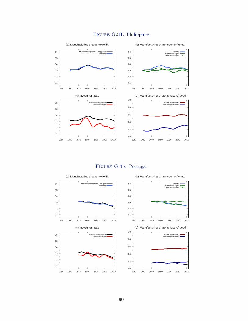
Figure G.34: Philippines
0.1
0.2
0.3
0.4
0.5
0.6
1950 1960 1970 1980 1990 2000 2010
(a) Manufacturing share: model fit
Manufacturing share: PhilippinesModel fit
0.1
0.2
0.3
0.4
0.5
0.6
1950 1960 1970 1980 1990 2000 2010
(b) Manufacturing share: counterfactual
Model fitIntensive margin
Extensive margin
0.1
0.2
0.3
0.4
0.5
0.6
1950 1960 1970 1980 1990 2000 2010
(c) Investment rate
Manufacturing shareInvestment rate
0.0
0.2
0.4
0.6
0.8
1.0
1950 1960 1970 1980 1990 2000 2010
(d) Manufacturing share by type of good
Within investmentWithin consumption
Figure G.35: Portugal
0.1
0.2
0.3
0.4
0.5
0.6
1950 1960 1970 1980 1990 2000 2010
(a) Manufacturing share: model fit
Manufacturing share: PortugalModel fit
0.1
0.2
0.3
0.4
0.5
0.6
1950 1960 1970 1980 1990 2000 2010
(b) Manufacturing share: counterfactual
Model fitIntensive margin
Extensive margin
0.1
0.2
0.3
0.4
0.5
0.6
1950 1960 1970 1980 1990 2000 2010
(c) Investment rate
Manufacturing shareInvestment rate
0.0
0.2
0.4
0.6
0.8
1.0
1950 1960 1970 1980 1990 2000 2010
(d) Manufacturing share by type of good
Within investmentWithin consumption
90
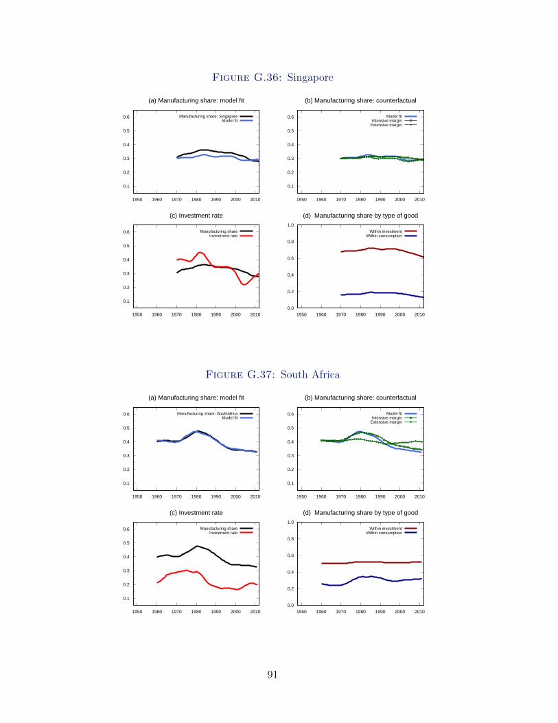
Figure G.36: Singapore
0.1
0.2
0.3
0.4
0.5
0.6
1950 1960 1970 1980 1990 2000 2010
(a) Manufacturing share: model fit
Manufacturing share: SingaporeModel fit
0.1
0.2
0.3
0.4
0.5
0.6
1950 1960 1970 1980 1990 2000 2010
(b) Manufacturing share: counterfactual
Model fitIntensive margin
Extensive margin
0.1
0.2
0.3
0.4
0.5
0.6
1950 1960 1970 1980 1990 2000 2010
(c) Investment rate
Manufacturing shareInvestment rate
0.0
0.2
0.4
0.6
0.8
1.0
1950 1960 1970 1980 1990 2000 2010
(d) Manufacturing share by type of good
Within investmentWithin consumption
Figure G.37: South Africa
0.1
0.2
0.3
0.4
0.5
0.6
1950 1960 1970 1980 1990 2000 2010
(a) Manufacturing share: model fit
Manufacturing share: SouthafricaModel fit
0.1
0.2
0.3
0.4
0.5
0.6
1950 1960 1970 1980 1990 2000 2010
(b) Manufacturing share: counterfactual
Model fitIntensive margin
Extensive margin
0.1
0.2
0.3
0.4
0.5
0.6
1950 1960 1970 1980 1990 2000 2010
(c) Investment rate
Manufacturing shareInvestment rate
0.0
0.2
0.4
0.6
0.8
1.0
1950 1960 1970 1980 1990 2000 2010
(d) Manufacturing share by type of good
Within investmentWithin consumption
91

Figure G.38: South Korea
0.1
0.2
0.3
0.4
0.5
0.6
1950 1960 1970 1980 1990 2000 2010
(a) Manufacturing share: model fit
Manufacturing share: SouthkoreaModel fit
0.1
0.2
0.3
0.4
0.5
0.6
1950 1960 1970 1980 1990 2000 2010
(b) Manufacturing share: counterfactual
Model fitIntensive margin
Extensive margin
0.1
0.2
0.3
0.4
0.5
0.6
1950 1960 1970 1980 1990 2000 2010
(c) Investment rate
Manufacturing shareInvestment rate
0.0
0.2
0.4
0.6
0.8
1.0
1950 1960 1970 1980 1990 2000 2010
(d) Manufacturing share by type of good
Within investmentWithin consumption
Figure G.39: Spain
0.1
0.2
0.3
0.4
0.5
0.6
1950 1960 1970 1980 1990 2000 2010
(a) Manufacturing share: model fit
Manufacturing share: SpainModel fit
0.1
0.2
0.3
0.4
0.5
0.6
1950 1960 1970 1980 1990 2000 2010
(b) Manufacturing share: counterfactual
Model fitIntensive margin
Extensive margin
0.1
0.2
0.3
0.4
0.5
0.6
1950 1960 1970 1980 1990 2000 2010
(c) Investment rate
Manufacturing shareInvestment rate
0.0
0.2
0.4
0.6
0.8
1.0
1950 1960 1970 1980 1990 2000 2010
(d) Manufacturing share by type of good
Within investmentWithin consumption
92
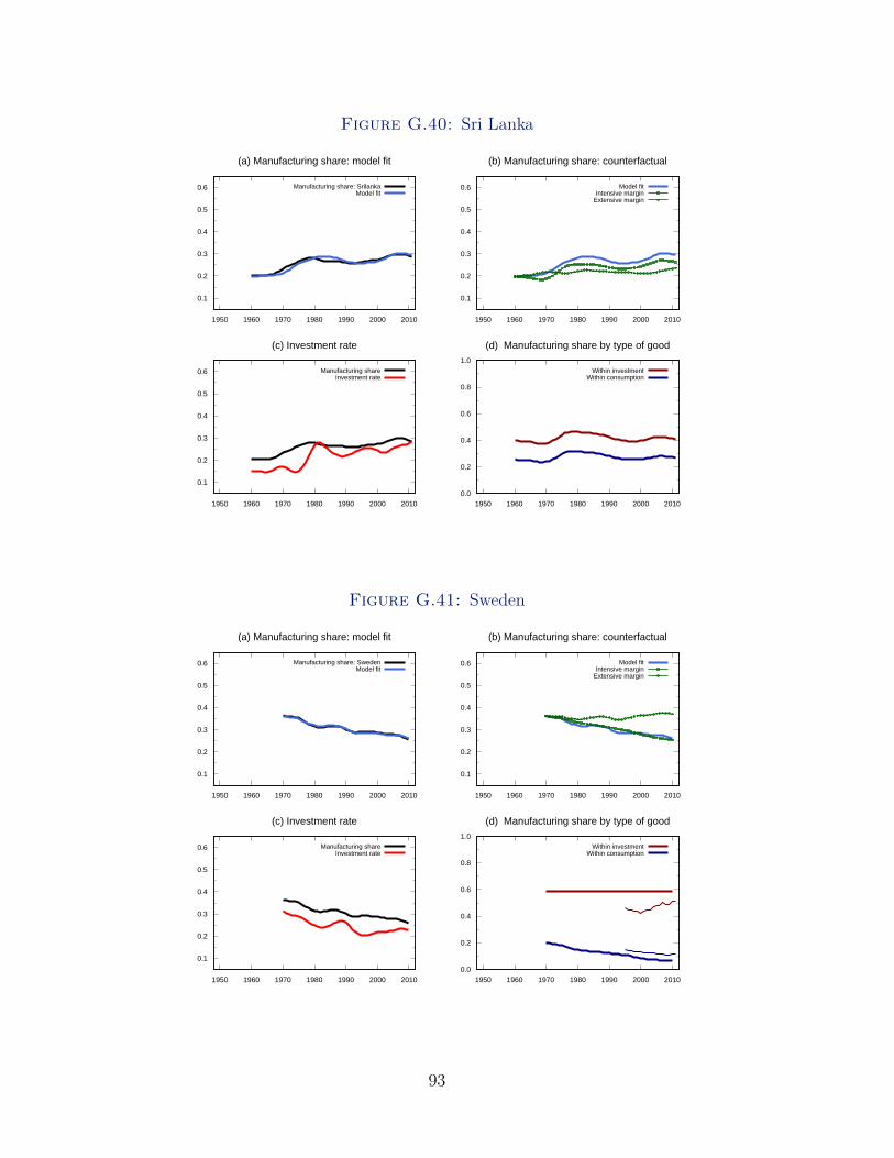
Figure G.40: Sri Lanka
0.1
0.2
0.3
0.4
0.5
0.6
1950 1960 1970 1980 1990 2000 2010
(a) Manufacturing share: model fit
Manufacturing share: SrilankaModel fit
0.1
0.2
0.3
0.4
0.5
0.6
1950 1960 1970 1980 1990 2000 2010
(b) Manufacturing share: counterfactual
Model fitIntensive margin
Extensive margin
0.1
0.2
0.3
0.4
0.5
0.6
1950 1960 1970 1980 1990 2000 2010
(c) Investment rate
Manufacturing shareInvestment rate
0.0
0.2
0.4
0.6
0.8
1.0
1950 1960 1970 1980 1990 2000 2010
(d) Manufacturing share by type of good
Within investmentWithin consumption
Figure G.41: Sweden
0.1
0.2
0.3
0.4
0.5
0.6
1950 1960 1970 1980 1990 2000 2010
(a) Manufacturing share: model fit
Manufacturing share: SwedenModel fit
0.1
0.2
0.3
0.4
0.5
0.6
1950 1960 1970 1980 1990 2000 2010
(b) Manufacturing share: counterfactual
Model fitIntensive margin
Extensive margin
0.1
0.2
0.3
0.4
0.5
0.6
1950 1960 1970 1980 1990 2000 2010
(c) Investment rate
Manufacturing shareInvestment rate
0.0
0.2
0.4
0.6
0.8
1.0
1950 1960 1970 1980 1990 2000 2010
(d) Manufacturing share by type of good
Within investmentWithin consumption
93
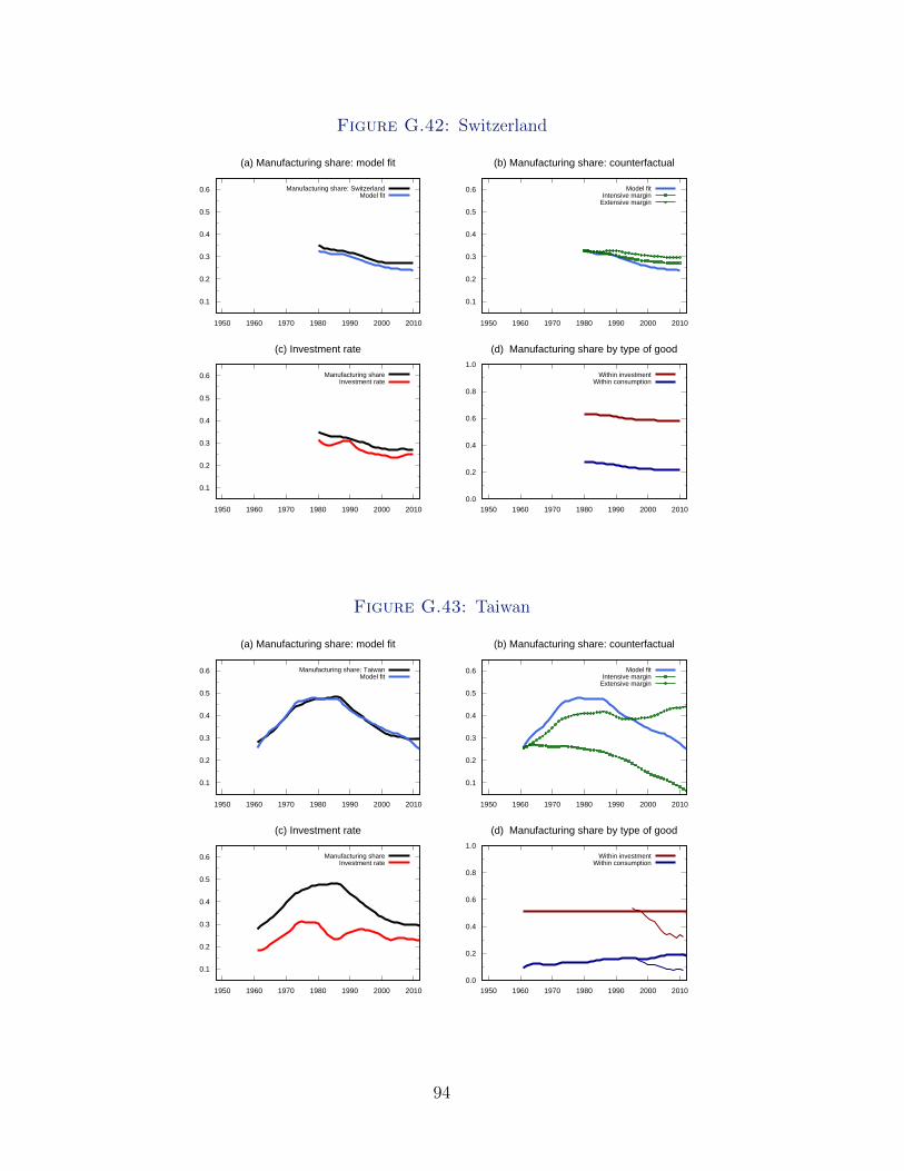
Figure G.42: Switzerland
0.1
0.2
0.3
0.4
0.5
0.6
1950 1960 1970 1980 1990 2000 2010
(a) Manufacturing share: model fit
Manufacturing share: SwitzerlandModel fit
0.1
0.2
0.3
0.4
0.5
0.6
1950 1960 1970 1980 1990 2000 2010
(b) Manufacturing share: counterfactual
Model fitIntensive margin
Extensive margin
0.1
0.2
0.3
0.4
0.5
0.6
1950 1960 1970 1980 1990 2000 2010
(c) Investment rate
Manufacturing shareInvestment rate
0.0
0.2
0.4
0.6
0.8
1.0
1950 1960 1970 1980 1990 2000 2010
(d) Manufacturing share by type of good
Within investmentWithin consumption
Figure G.43: Taiwan
0.1
0.2
0.3
0.4
0.5
0.6
1950 1960 1970 1980 1990 2000 2010
(a) Manufacturing share: model fit
Manufacturing share: TaiwanModel fit
0.1
0.2
0.3
0.4
0.5
0.6
1950 1960 1970 1980 1990 2000 2010
(b) Manufacturing share: counterfactual
Model fitIntensive margin
Extensive margin
0.1
0.2
0.3
0.4
0.5
0.6
1950 1960 1970 1980 1990 2000 2010
(c) Investment rate
Manufacturing shareInvestment rate
0.0
0.2
0.4
0.6
0.8
1.0
1950 1960 1970 1980 1990 2000 2010
(d) Manufacturing share by type of good
Within investmentWithin consumption
94

Figure G.44: Thailand
0.1
0.2
0.3
0.4
0.5
0.6
1950 1960 1970 1980 1990 2000 2010
(a) Manufacturing share: model fit
Manufacturing share: ThailandModel fit
0.1
0.2
0.3
0.4
0.5
0.6
1950 1960 1970 1980 1990 2000 2010
(b) Manufacturing share: counterfactual
Model fitIntensive margin
Extensive margin
0.1
0.2
0.3
0.4
0.5
0.6
1950 1960 1970 1980 1990 2000 2010
(c) Investment rate
Manufacturing shareInvestment rate
0.0
0.2
0.4
0.6
0.8
1.0
1950 1960 1970 1980 1990 2000 2010
(d) Manufacturing share by type of good
Within investmentWithin consumption
Figure G.45: Tunisia
0.1
0.2
0.3
0.4
0.5
0.6
1950 1960 1970 1980 1990 2000 2010
(a) Manufacturing share: model fit
Manufacturing share: TunisiaModel fit
0.1
0.2
0.3
0.4
0.5
0.6
1950 1960 1970 1980 1990 2000 2010
(b) Manufacturing share: counterfactual
Model fitIntensive margin
Extensive margin
0.1
0.2
0.3
0.4
0.5
0.6
1950 1960 1970 1980 1990 2000 2010
(c) Investment rate
Manufacturing shareInvestment rate
0.0
0.2
0.4
0.6
0.8
1.0
1950 1960 1970 1980 1990 2000 2010
(d) Manufacturing share by type of good
Within investmentWithin consumption
95

Figure G.46: Turkey
0.1
0.2
0.3
0.4
0.5
0.6
1950 1960 1970 1980 1990 2000 2010
(a) Manufacturing share: model fit
Manufacturing share: TurkeyModel fit
0.1
0.2
0.3
0.4
0.5
0.6
1950 1960 1970 1980 1990 2000 2010
(b) Manufacturing share: counterfactual
Model fitIntensive margin
Extensive margin
0.1
0.2
0.3
0.4
0.5
0.6
1950 1960 1970 1980 1990 2000 2010
(c) Investment rate
Manufacturing shareInvestment rate
0.0
0.2
0.4
0.6
0.8
1.0
1950 1960 1970 1980 1990 2000 2010
(d) Manufacturing share by type of good
Within investmentWithin consumption
Figure G.47: United Kingdom
0.1
0.2
0.3
0.4
0.5
0.6
1950 1960 1970 1980 1990 2000 2010
(a) Manufacturing share: model fit
Manufacturing share: UnitedkingdomModel fit
0.1
0.2
0.3
0.4
0.5
0.6
1950 1960 1970 1980 1990 2000 2010
(b) Manufacturing share: counterfactual
Model fitIntensive margin
Extensive margin
0.1
0.2
0.3
0.4
0.5
0.6
1950 1960 1970 1980 1990 2000 2010
(c) Investment rate
Manufacturing shareInvestment rate
0.0
0.2
0.4
0.6
0.8
1.0
1950 1960 1970 1980 1990 2000 2010
(d) Manufacturing share by type of good
Within investmentWithin consumption
96
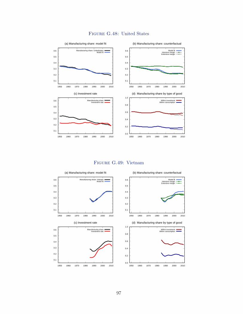
Figure G.48: United States
0.1
0.2
0.3
0.4
0.5
0.6
1950 1960 1970 1980 1990 2000 2010
(a) Manufacturing share: model fit
Manufacturing share: UnitedstatesModel fit
0.1
0.2
0.3
0.4
0.5
0.6
1950 1960 1970 1980 1990 2000 2010
(b) Manufacturing share: counterfactual
Model fitIntensive margin
Extensive margin
0.1
0.2
0.3
0.4
0.5
0.6
1950 1960 1970 1980 1990 2000 2010
(c) Investment rate
Manufacturing shareInvestment rate
0.0
0.2
0.4
0.6
0.8
1.0
1950 1960 1970 1980 1990 2000 2010
(d) Manufacturing share by type of good
Within investmentWithin consumption
Figure G.49: Vietnam
0.1
0.2
0.3
0.4
0.5
0.6
1950 1960 1970 1980 1990 2000 2010
(a) Manufacturing share: model fit
Manufacturing share: VietnamModel fit
0.1
0.2
0.3
0.4
0.5
0.6
1950 1960 1970 1980 1990 2000 2010
(b) Manufacturing share: counterfactual
Model fitIntensive margin
Extensive margin
0.1
0.2
0.3
0.4
0.5
0.6
1950 1960 1970 1980 1990 2000 2010
(c) Investment rate
Manufacturing shareInvestment rate
0.0
0.2
0.4
0.6
0.8
1.0
1950 1960 1970 1980 1990 2000 2010
(d) Manufacturing share by type of good
Within investmentWithin consumption
97
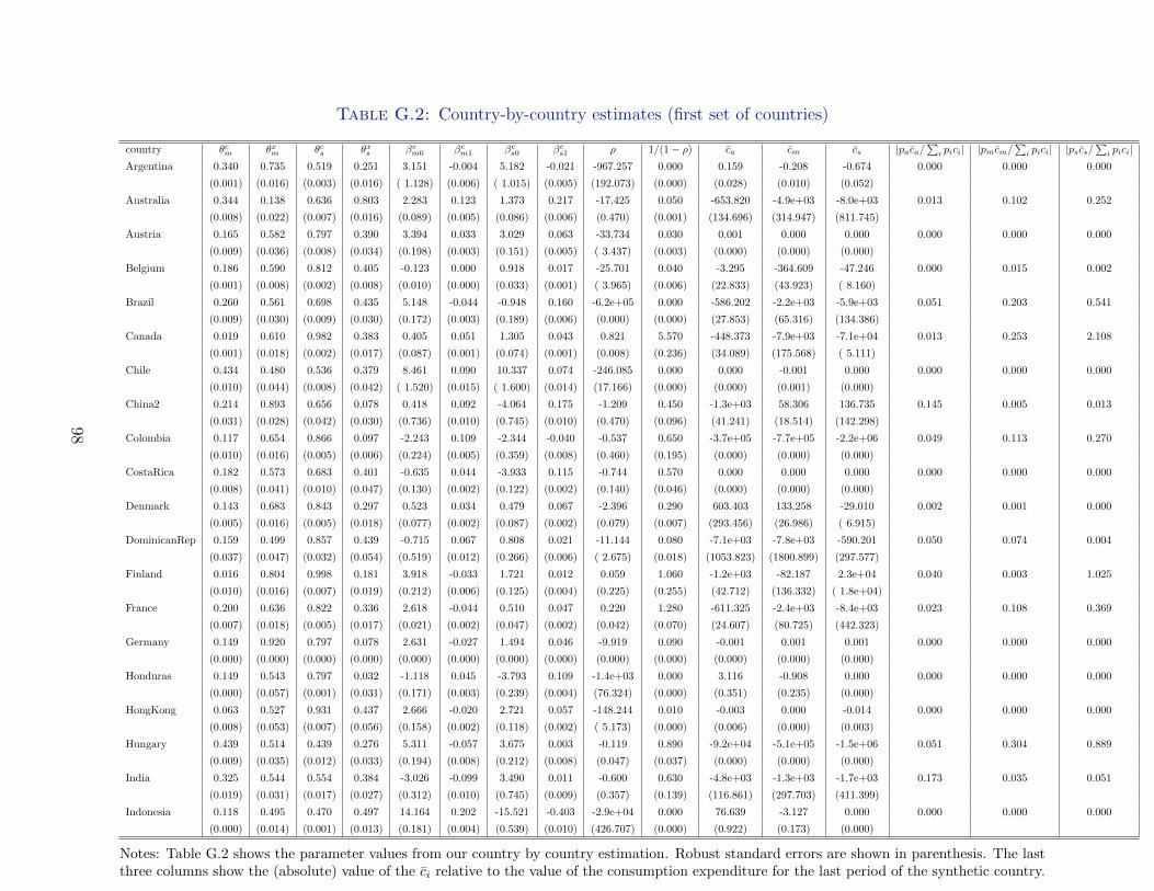
Table G.2: Country-by-country estimates (first set of countries)
country θcm θxm θcs θxs βem0 βem1 βes0 βes1 ρ 1/(1− ρ) ca cm cs |paca/∑i pici| |pmcm/
∑i pici| |pscs/
∑i pici|
Argentina 0.340 0.735 0.519 0.251 3.151 -0.004 5.182 -0.021 -967.257 0.000 0.159 -0.208 -0.674 0.000 0.000 0.000
(0.001) (0.016) (0.003) (0.016) ( 1.128) (0.006) ( 1.015) (0.005) (192.073) (0.000) (0.028) (0.010) (0.052)
Australia 0.344 0.138 0.636 0.803 2.283 0.123 1.373 0.217 -17.425 0.050 -653.820 -4.9e+03 -8.0e+03 0.013 0.102 0.252
(0.008) (0.022) (0.007) (0.016) (0.089) (0.005) (0.086) (0.006) (0.470) (0.001) (134.696) (314.947) (811.745)
Austria 0.165 0.582 0.797 0.390 3.394 0.033 3.029 0.063 -33.734 0.030 0.001 0.000 0.000 0.000 0.000 0.000
(0.009) (0.036) (0.008) (0.034) (0.198) (0.003) (0.151) (0.005) ( 3.437) (0.003) (0.000) (0.000) (0.000)
Belgium 0.186 0.590 0.812 0.405 -0.123 0.000 0.918 0.017 -25.701 0.040 -3.295 -364.609 -47.246 0.000 0.015 0.002
(0.001) (0.008) (0.002) (0.008) (0.010) (0.000) (0.033) (0.001) ( 3.965) (0.006) (22.833) (43.923) ( 8.160)
Brazil 0.260 0.561 0.698 0.435 5.148 -0.044 -0.948 0.160 -6.2e+05 0.000 -586.202 -2.2e+03 -5.9e+03 0.051 0.203 0.541
(0.009) (0.030) (0.009) (0.030) (0.172) (0.003) (0.189) (0.006) (0.000) (0.000) (27.853) (65.316) (134.386)
Canada 0.019 0.610 0.982 0.383 0.405 0.051 1.305 0.043 0.821 5.570 -448.373 -7.9e+03 -7.1e+04 0.013 0.253 2.108
(0.001) (0.018) (0.002) (0.017) (0.087) (0.001) (0.074) (0.001) (0.008) (0.236) (34.089) (175.568) ( 5.111)
Chile 0.434 0.480 0.536 0.379 8.461 0.090 10.337 0.074 -246.085 0.000 0.000 -0.001 0.000 0.000 0.000 0.000
(0.010) (0.044) (0.008) (0.042) ( 1.520) (0.015) ( 1.600) (0.014) (17.166) (0.000) (0.000) (0.001) (0.000)
China2 0.214 0.893 0.656 0.078 0.418 0.092 -4.064 0.175 -1.209 0.450 -1.3e+03 58.306 136.735 0.145 0.005 0.013
(0.031) (0.028) (0.042) (0.030) (0.736) (0.010) (0.745) (0.010) (0.470) (0.096) (41.241) (18.514) (142.298)
Colombia 0.117 0.654 0.866 0.097 -2.243 0.109 -2.344 -0.040 -0.537 0.650 -3.7e+05 -7.7e+05 -2.2e+06 0.049 0.113 0.270
(0.010) (0.016) (0.005) (0.006) (0.224) (0.005) (0.359) (0.008) (0.460) (0.195) (0.000) (0.000) (0.000)
CostaRica 0.182 0.573 0.683 0.401 -0.635 0.044 -3.933 0.115 -0.744 0.570 0.000 0.000 0.000 0.000 0.000 0.000
(0.008) (0.041) (0.010) (0.047) (0.130) (0.002) (0.122) (0.002) (0.140) (0.046) (0.000) (0.000) (0.000)
Denmark 0.143 0.683 0.843 0.297 0.523 0.034 0.479 0.067 -2.396 0.290 603.403 133.258 -29.010 0.002 0.001 0.000
(0.005) (0.016) (0.005) (0.018) (0.077) (0.002) (0.087) (0.002) (0.079) (0.007) (293.456) (26.986) ( 6.915)
DominicanRep 0.159 0.499 0.857 0.439 -0.715 0.067 0.808 0.021 -11.144 0.080 -7.1e+03 -7.8e+03 -590.201 0.050 0.074 0.004
(0.037) (0.047) (0.032) (0.054) (0.519) (0.012) (0.266) (0.006) ( 2.675) (0.018) (1053.823) (1800.899) (297.577)
Finland 0.016 0.804 0.998 0.181 3.918 -0.033 1.721 0.012 0.059 1.060 -1.2e+03 -82.187 2.3e+04 0.040 0.003 1.025
(0.010) (0.016) (0.007) (0.019) (0.212) (0.006) (0.125) (0.004) (0.225) (0.255) (42.712) (136.332) ( 1.8e+04)
France 0.200 0.636 0.822 0.336 2.618 -0.044 0.510 0.047 0.220 1.280 -611.325 -2.4e+03 -8.4e+03 0.023 0.108 0.369
(0.007) (0.018) (0.005) (0.017) (0.021) (0.002) (0.047) (0.002) (0.042) (0.070) (24.607) (80.725) (442.323)
Germany 0.149 0.920 0.797 0.078 2.631 -0.027 1.494 0.046 -9.919 0.090 -0.001 0.001 0.001 0.000 0.000 0.000
(0.000) (0.000) (0.000) (0.000) (0.000) (0.000) (0.000) (0.000) (0.000) (0.000) (0.000) (0.000) (0.000)
Honduras 0.149 0.543 0.797 0.032 -1.118 0.045 -3.793 0.109 -1.4e+03 0.000 3.116 -0.908 0.000 0.000 0.000 0.000
(0.000) (0.057) (0.001) (0.031) (0.171) (0.003) (0.239) (0.004) (76.324) (0.000) (0.351) (0.235) (0.000)
HongKong 0.063 0.527 0.931 0.437 2.666 -0.020 2.721 0.057 -148.244 0.010 -0.003 0.000 -0.014 0.000 0.000 0.000
(0.008) (0.053) (0.007) (0.056) (0.158) (0.002) (0.118) (0.002) ( 5.173) (0.000) (0.006) (0.000) (0.003)
Hungary 0.439 0.514 0.439 0.276 5.311 -0.057 3.675 0.003 -0.119 0.890 -9.2e+04 -5.1e+05 -1.5e+06 0.051 0.304 0.889
(0.009) (0.035) (0.012) (0.033) (0.194) (0.008) (0.212) (0.008) (0.047) (0.037) (0.000) (0.000) (0.000)
India 0.325 0.544 0.554 0.384 -3.026 -0.099 3.490 0.011 -0.600 0.630 -4.8e+03 -1.3e+03 -1.7e+03 0.173 0.035 0.051
(0.019) (0.031) (0.017) (0.027) (0.312) (0.010) (0.745) (0.009) (0.357) (0.139) (116.861) (297.703) (411.399)
Indonesia 0.118 0.495 0.470 0.497 14.164 0.202 -15.521 -0.403 -2.9e+04 0.000 76.639 -3.127 0.000 0.000 0.000 0.000
(0.000) (0.014) (0.001) (0.013) (0.181) (0.004) (0.539) (0.010) (426.707) (0.000) (0.922) (0.173) (0.000)
Notes: Table G.2 shows the parameter values from our country by country estimation. Robust standard errors are shown in parenthesis. The lastthree columns show the (absolute) value of the ci relative to the value of the consumption expenditure for the last period of the synthetic country.
98
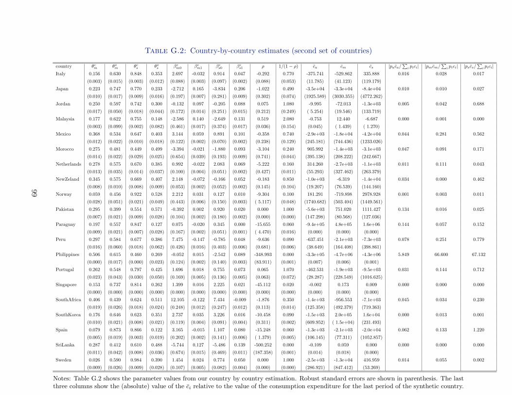
Table G.2: Country-by-country estimates (second set of countries)
country θcm θxm θcs θxs βem0 βem1 βes0 βes1 ρ 1/(1− ρ) ca cm cs |paca/∑i pici| |pmcm/
∑i pici| |pscs/
∑i pici|
Italy 0.156 0.630 0.848 0.353 2.697 -0.032 0.914 0.047 -0.292 0.770 -375.741 -529.862 335.888 0.016 0.028 0.017
(0.003) (0.015) (0.003) (0.012) (0.088) (0.003) (0.097) (0.002) (0.088) (0.053) (11.785) (41.123) (119.179)
Japan 0.223 0.747 0.770 0.233 -2.712 0.165 -3.834 0.206 -1.022 0.490 -3.5e+04 -3.3e+04 -8.4e+04 0.010 0.010 0.027
(0.010) (0.017) (0.009) (0.016) (0.197) (0.007) (0.281) (0.009) (0.302) (0.074) (1925.589) (3030.355) (4772.262)
Jordan 0.250 0.597 0.742 0.300 -0.132 0.097 -0.205 0.088 0.075 1.080 -9.995 -72.013 -1.3e+03 0.005 0.042 0.688
(0.017) (0.050) (0.018) (0.044) (0.172) (0.014) (0.251) (0.015) (0.212) (0.249) ( 5.254) (19.546) (133.719)
Malaysia 0.177 0.622 0.755 0.148 -2.586 0.140 -2.649 0.131 0.519 2.080 -0.753 12.440 -6.687 0.000 0.001 0.000
(0.003) (0.099) (0.002) (0.082) (0.461) (0.017) (0.374) (0.017) (0.036) (0.154) (0.045) ( 1.439) ( 1.270)
Mexico 0.368 0.534 0.647 0.403 3.144 0.059 0.891 0.101 -0.358 0.740 -2.9e+03 -1.8e+04 -4.2e+04 0.044 0.281 0.562
(0.012) (0.022) (0.010) (0.018) (0.122) (0.002) (0.070) (0.002) (0.238) (0.129) (245.181) (744.436) (1233.026)
Morocco 0.275 0.481 0.449 0.499 -3.394 -0.021 -1.880 0.093 -3.104 0.240 905.992 -1.4e+03 -3.1e+03 0.047 0.091 0.171
(0.014) (0.022) (0.029) (0.025) (0.654) (0.039) (0.193) (0.009) (0.741) (0.044) (395.138) (208.222) (242.667)
Netherlands 0.278 0.575 0.670 0.385 0.992 -0.022 2.083 0.069 -5.222 0.160 314.260 -2.7e+03 -1.1e+03 0.011 0.111 0.043
(0.013) (0.035) (0.014) (0.037) (0.100) (0.004) (0.051) (0.002) (0.427) (0.011) (55.293) (327.462) (263.379)
NewZeland 0.345 0.575 0.669 0.407 2.148 -0.072 -0.166 0.052 -0.183 0.850 -1.0e+03 -6.319 -1.4e+04 0.034 0.000 0.462
(0.008) (0.010) (0.008) (0.009) (0.053) (0.002) (0.052) (0.002) (0.145) (0.104) (19.207) (76.539) (144.160)
Norway 0.059 0.456 0.922 0.528 2.212 0.031 0.127 0.010 -9.304 0.100 181.291 -719.898 2978.928 0.001 0.003 0.011
(0.028) (0.051) (0.021) (0.049) (0.443) (0.006) (0.150) (0.003) ( 5.117) (0.048) (1740.682) (503.404) (1449.561)
Pakistan 0.295 0.399 0.554 0.571 -0.392 0.002 0.920 0.020 0.000 1.000 -5.6e+03 751.020 1111.427 0.134 0.016 0.025
(0.007) (0.021) (0.009) (0.028) (0.104) (0.002) (0.180) (0.002) (0.000) (0.000) (147.298) (80.568) (127.036)
Paraguay 0.197 0.557 0.847 0.127 0.075 -0.020 0.345 0.000 -15.655 0.060 -9.4e+05 4.8e+05 1.6e+06 0.144 0.057 0.152
(0.009) (0.021) (0.007) (0.028) (0.167) (0.002) (0.051) (0.001) ( 4.470) (0.016) (0.000) (0.000) (0.000)
Peru 0.297 0.584 0.677 0.386 7.475 -0.147 -0.785 0.048 -9.636 0.090 -637.451 -2.1e+03 -7.3e+03 0.078 0.251 0.779
(0.016) (0.060) (0.018) (0.062) (0.426) (0.016) (0.403) (0.006) (0.681) (0.006) (38.649) (164.408) (398.861)
Philippines 0.506 0.615 0.460 0.269 -0.052 0.015 -2.542 0.089 -348.993 0.000 -3.3e+05 -4.7e+06 -4.3e+06 5.849 66.600 67.132
(0.000) (0.017) (0.000) (0.023) (0.124) (0.002) (0.140) (0.003) (83.911) (0.001) (0.007) (0.006) (0.001)
Portugal 0.262 0.548 0.797 0.425 1.696 0.018 0.755 0.073 0.065 1.070 -462.531 -1.9e+03 -9.5e+03 0.031 0.144 0.712
(0.023) (0.043) (0.030) (0.050) (0.169) (0.005) (0.136) (0.005) (0.063) (0.072) (28.287) (228.549) (1016.625)
Singapore 0.153 0.737 0.814 0.262 1.399 0.016 2.225 0.021 -45.112 0.020 -0.002 0.173 0.009 0.000 0.000 0.000
(0.000) (0.000) (0.000) (0.000) (0.000) (0.000) (0.000) (0.000) (0.000) (0.000) (0.000) (0.000) (0.000)
SouthAfrica 0.406 0.439 0.624 0.511 12.105 -0.122 7.434 -0.009 -1.876 0.350 -1.4e+03 -956.553 -7.1e+03 0.045 0.034 0.230
(0.019) (0.026) (0.018) (0.024) (0.248) (0.012) (0.247) (0.012) (0.113) (0.014) (125.358) (492.379) (719.363)
SouthKorea 0.176 0.646 0.623 0.351 2.737 0.035 3.226 0.016 -10.458 0.090 -1.5e+03 2.0e+05 1.6e+04 0.000 0.013 0.001
(0.010) (0.021) (0.008) (0.021) (0.119) (0.004) (0.091) (0.004) (0.311) (0.002) (609.952) ( 1.5e+04) (231.493)
Spain 0.079 0.873 0.866 0.122 3.165 -0.015 1.107 0.080 -15.248 0.060 -1.3e+03 -2.1e+03 -2.0e+04 0.062 0.133 1.220
(0.005) (0.019) (0.003) (0.019) (0.202) (0.002) (0.141) (0.006) ( 1.379) (0.005) (106.145) (77.311) (1052.857)
SriLanka 0.287 0.412 0.610 0.488 -5.744 0.127 -5.486 0.139 -500.252 0.000 -0.109 0.059 0.000 0.000 0.000 0.000
(0.011) (0.042) (0.008) (0.036) (0.674) (0.015) (0.469) (0.011) (187.358) (0.001) (0.014) (0.018) (0.000)
Sweden 0.026 0.590 0.984 0.390 1.454 0.024 0.774 0.050 0.000 1.000 -2.5e+03 -1.3e+04 416.959 0.014 0.055 0.002
(0.009) (0.026) (0.009) (0.028) (0.107) (0.005) (0.082) (0.004) (0.000) (0.000) (286.921) (847.412) (53.269)
Notes: Table G.2 shows the parameter values from our country by country estimation. Robust standard errors are shown in parenthesis. The lastthree columns show the (absolute) value of the ci relative to the value of the consumption expenditure for the last period of the synthetic country.
99
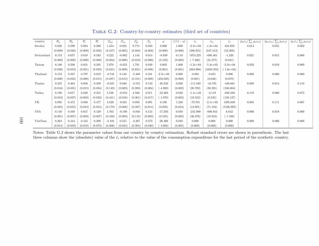
Table G.2: Country-by-country estimates (third set of countries)
country θcm θxm θcs θxs βem0 βem1 βes0 βes1 ρ 1/(1− ρ) ca cm cs |paca/∑i pitcit| |pmcm/
∑i pitcit| |pscs/
∑i pitcit|
Sweden 0.026 0.590 0.984 0.390 1.454 0.024 0.774 0.050 0.000 1.000 -2.5e+03 -1.3e+04 416.959 0.014 0.055 0.002
(0.009) (0.026) (0.009) (0.028) (0.107) (0.005) (0.082) (0.004) (0.000) (0.000) (286.921) (847.412) (53.269)
Switzerland 0.153 0.657 0.818 0.343 0.222 -0.002 1.144 0.014 -8.039 0.110 1074.325 -686.461 -1.320 0.021 0.015 0.000
(0.000) (0.000) (0.000) (0.000) (0.004) (0.000) (0.010) (0.000) (0.192) (0.002) ( 7.408) (31.875) (0.041)
Taiwan 0.186 0.509 0.831 0.385 5.970 -0.052 1.791 0.049 0.003 1.000 -1.2e+04 -5.4e+03 -3.2e+04 0.033 0.010 0.069
(0.030) (0.053) (0.031) (0.050) (0.621) (0.009) (0.621) (0.008) (0.001) (0.001) (664.968) (2483.352) ( 1.6e+04)
Thailand 0.152 0.507 0.797 0.019 -3.743 0.148 -5.480 0.161 -2.5e+03 0.000 -0.001 -0.051 0.696 0.000 0.000 0.000
(0.000) (0.032) (0.000) (0.015) (0.287) (0.012) (0.181) (0.009) (456.695) (0.000) (0.001) (0.046) (0.078)
Tunisia 0.225 0.464 0.656 0.509 -0.025 0.040 -3.555 0.133 -46.332 0.020 -111.840 -44.791 -446.661 0.028 0.014 0.110
(0.016) (0.031) (0.015) (0.034) (0.149) (0.003) (0.203) (0.004) ( 4.269) (0.002) (20.702) (38.201) (106.004)
Turkey 0.196 0.617 0.820 0.355 5.538 -0.010 4.586 0.011 -22.268 0.040 -1.1e+03 -3.119 -638.286 0.119 0.000 0.072
(0.010) (0.037) (0.003) (0.033) (0.441) (0.016) (0.361) (0.017) ( 1.670) (0.003) (19.552) (0.535) (128.127)
UK 0.095 0.472 0.898 0.477 4.829 -0.021 0.059 0.091 0.196 1.240 -70.701 -2.1e+03 1295.638 0.005 0.111 0.067
(0.025) (0.052) (0.024) (0.054) (0.179) (0.008) (0.387) (0.014) (0.028) (0.044) (13.991) (71.104) (1526.995)
USA 0.146 0.569 0.857 0.429 4.763 -0.100 -0.856 0.124 -17.293 0.050 -245.000 -690.943 6.042 0.006 0.019 0.000
(0.001) (0.007) (0.003) (0.007) (0.160) (0.003) (0.145) (0.003) (0.535) (0.002) (36.376) (16.943) ( 1.166)
VietNam 0.264 0.444 0.445 0.206 -3.102 0.315 -2.387 0.273 -26.466 0.040 0.000 0.000 0.000 0.000 0.000 0.000
(0.014) (0.059) (0.018) (0.073) (0.306) (0.034) (0.304) (0.030) ( 4.002) (0.005) (0.000) (0.000) (0.000)
Notes: Table G.2 shows the parameter values from our country by country estimation. Robust standard errors are shown in parenthesis. The lastthree columns show the (absolute) value of the ci relative to the value of the consumption expenditure for the last period of the synthetic country.
100