investment in the euro area: why has it been weak? · although investment in the euro area could...
TRANSCRIPT

WP/15/32
Investment in the Euro Area: Why Has It Been
Weak?
Bergljot Barkbu, S. Pelin Berkmen, Pavel Lukyantsau, Sergejs
Saksonovs, and Hanni Schoelermann

© 2015 International Monetary Fund WP/15/32
IMF Working Paper
European Department
Investment in the Euro Area: Why Has It Been Weak?
Prepared by Bergljot Barkbu, S. Pelin Berkmen, Pavel Lukyantsau, Sergejs Saksonovs,
and Hanni Schoelermann
Authorized for distribution by Petya Koeva Brooks
February 2015
Abstract
Investment across the euro area remains below its pre-crisis level. Its performance has
been weaker than in most previous recessions and financial crises. This paper shows that a
part of this weakness can be explained by output dynamics, particularly before the
European sovereign debt crisis. The rest is explained by a high cost of capital, financial
constraints, corporate leverage, and uncertainty. There is a considerable cross country
heterogeneity in terms of both investment dymanics and its determinants. Based on the
findings of this paper, investment is expected to pick up as the recovery strengthens and
uncertainty declines, but persistent financial fragmentation and high corporate leverage in
some countries will likely continue to weigh on investment.
JEL Classification Numbers: E22, E51
Keywords: Investment, cost of capital, credit rationing
Authors’ E-Mail Addresses: [email protected]; [email protected];
[email protected]; [email protected]; [email protected].
This Working Paper should not be reported as representing the views of the IMF.
The views expressed in this Working Paper are those of the author(s) and do not necessarily
represent those of the IMF or IMF policy. Working Papers describe research in progress by the
author(s) and are published to elicit comments and to further debate.

3
Contents Page
I. Introduction ............................................................................................................................4
II. Literature Survey ...................................................................................................................7
III. Drivers of Investment in the Euro Area ...............................................................................8 A. Output Changes and the Real Cost of Capital...........................................................9 B. Additional Determinants of Investment ..................................................................10
C. Accelerator + Model: Exploring Other Determinants of Investment ......................12
IV. The Magnitude of Missing Investment ..............................................................................15
V. Conclusion ..........................................................................................................................16
References ...............................................................................................................................17
Appendices
1. Data Definitions and Sources...............................................................................................19 2. Results ..................................................................................................................................22
Figures
A1.1. Cost of Capital Calculations ........................................................................................21
A2.1. Accelerator Model: Private Non-residential Investment/Capital Ratio .......................23
A2.2. Neoclassical Model Without Financial Constrains: Private Non-residential Investment
to Capital Ratio ......................................................................................................................26
A2.3. Neoclassical Model with Financial Constrains: Private Non-residential Investment to
Capital Ratio .........................................................................................................................27
A2.4. Bond Market Model (Controlling for Output Changes and Financial Constraints) ....29
A2.5. Contributions to Change in Investment-to-Capital Ratio (Accelerator + Model,
cumulative) ............................................................................................................................30
Tables
A2.1. Accelerator Model- Total Investments (Newey-West HAC Standard.........................22
A2.2 Neoclassical Model: Estimates with Newey West Standard Errors .............................24
A2.3. Neoclassical Model Augmented with Financial Constrains: Estimates with Newey
West Standard Errors .............................................................................................................25
A2.4. Bond Market Model (Controlling for Output Changes and Financial Constraints) ....28
A2.5. Significance of Accelerator + Model ...........................................................................30

4
I. INTRODUCTION1
Investment in euro area countries has been hit hard since the onset of the crisis and has not
yet recovered, including in many of the core economies. Total investment in real terms
remains below its pre-crisis level across the euro area. While a part of this decline reflects
lower public and housing investment in certain countries,2 private non-residential investment
also remains well below its pre-crisis level particularly in stressed countries (see text charts).3
Sources: Eurostat, Haver Analytics; and staff calculations.
Sources: Eurostat, and staff calculations.
Notes: 1/ Last available data point: DEU = 2012Q4; PRT = 2013Q3.
Overall, the behavior of investment has varied substantially across the euro area and across
firm sizes. The decline in investment is larger in stressed economies than in core economies.
At the same time, the conditions for SMEs have worsened more than the conditions for larger
corporations. This heterogeneity could reflect various interacting factors, such as structural
differences between economies and a varying degree of vulnerabilities across countries (such
as bank-sovereign links, financial fragmentation, corporate indebtedness, and policy
uncertainities).
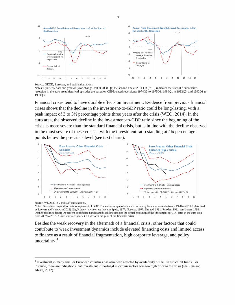
Weak investment performance in Europe has coincided with large output losses. Real GDP in
the euro area remains below its pre-crisis level, the output gap is negative and large, and the
recovery is more sluggish than in typical recessions. Given subdued output performance and
a weak growth outlook, it is not surprising that investment has also lagged behind the trend
observed in most previous recessions (see text charts).
1 This paper draws on the work that has been done in 2014 Euro Area Policies: Selected Issues (IMF, 2014). 2 For example, housing investment declined from about 12–13 percent of GDP before the crisis to about 6 percent of GDP in
Spain and to about 2–3 percent of GDP in Greece and Ireland after the crisis. 3 Stressed countries refer to debtor countries who have experienced high funding costs (public and private) and suffered
from financial fragmentation during the period covered. For the charts and regressions in this paper, data on private non-
residential investment are obtained from Eurostat to ensure consistency and comparability across countries. Looking into
other data sources also shows weak investment dynamics. For example, real fixed investment in equipment in Germany and
real investment by non-financial corporations in France, equipment and transportation machinery in the euro area are also
weaker than their pre-crisis levels.
0
20
40
60
80
100
120
GRC IRL ESP PRT ITA EA GBR FRA DEU USA
Investment Recovery to Date: 2013Q4(Percent; 2007 quarterly average=100)
0
20
40
60
80
100
120
PRT 1/ ITA GBR ESP EA DEU 1/ FRA
Private Non-Residential Investment Recovery to
Date: 2013Q4(Percent; 2007 quarterly average=100)
5
Source: OECD, Eurostat; and staff calculations.
Notes: Quarterly data and year-on-year change. t=0 at 2008 Q1; the second line at 2011 Q3 (t=15) indicates the start of a successive
recession in the euro area; historical episodes are based on CEPR-dated recessions: 1974Q3 to 1975Q1, 1980Q1 to 1982Q3, and 1992Q1 to
1993Q3.
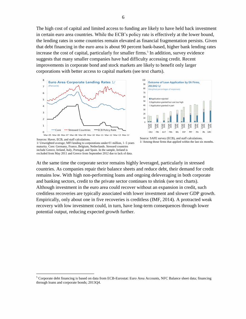
Financial crises tend to have durable effects on investment. Evidence from previous financial
crises shows that the decline in the investment-to-GDP ratio could be long-lasting, with a
peak impact of 3 to 3½ percentage points three years after the crisis (WEO, 2014). In the
euro area, the observed decline in the investment-to-GDP ratio since the beginning of the
crisis is more severe than the standard financial crisis, but is in line with the decline observed
in the most severe of these crises—with the investment ratio standing at 4¼ percentage
points below the pre-crisis level (see text charts).
Source: WEO (2014), and staff calculations.
Notes: Gross fixed capital formation in percent of GDP. The entire sample of advanced economy financial crises between 1970 and 2007 identified
by Laeven and Valencia (2012). Big 5 financial crises are those in Spain, 1977; Norway, 1987; Finland, 1991; Sweden, 1991; and Japan, 1992.
Dashed red lines denote 90 percent confidence bands; and black line denotes the actual evolution of the investment-to-GDP ratio in the euro area
from 2007 to 2013. X-axis units are years; t = 0 denotes the year of the financial crisis.
Besides the weak recovery in the aftermath of a financial crisis, other factors that could
contribute to weak investment dynamics include elevated financing costs and limited access
to finance as a result of financial fragmentation, high corporate leverage, and policy
uncertainty.4
4 Investment in many smaller European countries has also been affected by availability of the EU structural funds. For
instance, there are indications that investment in Portugal in certain sectors was too high prior to the crisis (see Pina and
Abreu, 2012).
-10
-5
0
5
10
-12 -9 -6 -3 0 3 6 9 12 15 18 21
Euro area historical
average (based on
3 episodes)
Current (t=0 at
2008Q1)
2008Q1
2011Q3
Annual GDP Growth Around Recessions, t=0 at the Start of
the Recession
-20
-15
-10
-5
0
5
10
15
-12 -9 -6 -3 0 3 6 9 12 15 18 21
Euro area historical
average (based on
3 episodes)
Current (t=0 at
2008Q1)
Annual Fixed Investment Growth Around Recessions, t=0 at
the Start of the Recession
2008Q1
2011Q3
-7
-6
-5
-4
-3
-2
-1
0
–1 0 1 2 3 4 5 6 7 8 9 10
Investment-to-GDP ratio - crisis episodes
90 percent confidence interval
EA: Investment to GDP, 2007–13 ( index, 2007 = 0)
Euro Area vs. Other Financial Crisis
Episodes(Percent of GDP)
-7
-6
-5
-4
-3
-2
-1
0
–1 0 1 2 3 4 5 6 7 8 9 10
Investment-to-GDP ratio - crisis episodes
90 percent convidence interval
EA: Investment to GDP, 2007–13 ( index, 2007 = 0)
Euro Area vs. Other Financial Crisis
Episodes (Big 5 crises)(Percent of GDP)
6
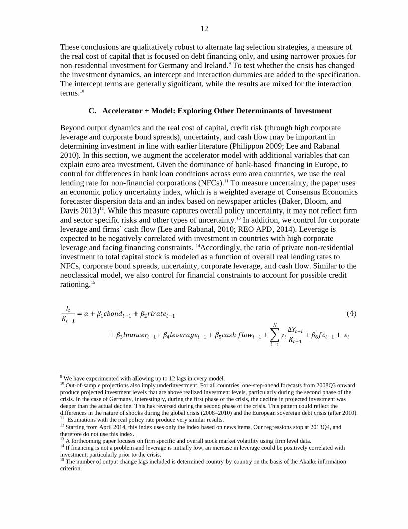
The high cost of capital and limited access to funding are likely to have held back investment
in certain euro area countries. While the ECB’s policy rate is effectively at the lower bound,
the lending rates in some countries remain elevated as financial fragmentation persists. Given
that debt financing in the euro area is about 90 percent bank-based, higher bank lending rates
increase the cost of capital, particularly for smaller firms.5 In addition, survey evidence
suggests that many smaller companies have had difficulty accessing credit. Recent
improvements in corporate bond and stock markets are likely to benefit only larger
corporations with better access to capital markets (see text charts).
Sources: Haver, ECB, and staff calculations.
1/ Unweighted average; MFI lending to corporations under €1 million, 1–5 years
maturity. Core: Germany, France, Belgium, Netherlands. Stressed countries
include Greece, Ireland, Italy, Portugal, and Spain. In the sample, Ireland is
excluded from May 2011 and Greece from September 2012 due to lack of data.
Source: SAFE survey (ECB), and staff calculations.
1/ Among those firms that applied within the last six months.
At the same time the corporate sector remains highly leveraged, particularly in stressed
countries. As companies repair their balance sheets and reduce debt, their demand for credit
remains low. With high non-performing loans and ongoing deleveraging in both corporate
and banking sectors, credit to the private sector continues to shrink (see text charts).
Although investment in the euro area could recover without an expansion in credit, such
creditless recoveries are typically associated with lower investment and slower GDP growth.
Empirically, only about one in five recoveries is creditless (IMF, 2014). A protracted weak
recovery with low investment could, in turn, have long-term consequences through lower
potential output, reducing expected growth further.
5 Corporate debt financing is based on data from ECB-Eurostat: Euro Area Accounts, NFC Balance sheet data; financing
through loans and corporate bonds; 2013Q4.
0
1
2
3
4
5
6
7
8
Mar-05 Mar-06 Mar-07 Mar-08 Mar-09 Mar-10 Mar-11 Mar-12 Mar-13 Mar-14
Core Stressed Countries ECB Policy Rate
Euro Area Corporate Lending Rates 1/ (Percent)
0
10
20
30
40
50
60
70
80
90
100
Larg
eSM
E
Larg
eSM
E
Larg
eSM
E
Larg
eSM
E
Larg
eSM
E
Larg
eSM
E
Larg
eSM
E
Larg
eSM
E
Larg
eSM
E
Larg
eSM
E
DEU FIN AUT FRA BEL ESP PRT ITA IRL GRC
Application rejected
Application granted but cost too high
Application granted in part
Outcome of Loan Application by EA Firms,
2013H2 1/(Weighted percentages of responses)

7
Source: ECB.
1/ Debt at euro area level is non-consolidated.
Source: Haver. The decline in the stock of credit for Slovenia at end-
2013 is in part due to the transfer of non-performing loans to BAMC.
Against this background, this paper explores the factors explaining non-residential
investment across the euro area. Weak recovery, financial fragmentation, high corporate
leverage, and policy uncertainty could all hold investment back. To identify the impact of
each factor, the paper uses three sets of models: i) an accelerator model (output changes);
ii) a neoclassical model (real cost of capital); and iii) an “accelerator +” model (output
changes, uncertainty, borrowing costs, leverage, and cash flow).
The paper finds that all of the above-mentioned factors have been important in explaining
weak investment, but with considerable differences among countries. The accelerator model
which relies only on output changes tracks investment closely, particularly for Spain, but
actual post-crisis investment has remained below its model-implied value for most countries.
The neoclassical model shows that, as expected, real cost of capital is a significant factor and
that financial constraints held back investment in some countries. Nevertheless, the actual
post-crisis investment is still below its estimated level for most countries. Finally, the
“accelerator +” model helps reduce this difference between actual and estimated investment.
Among other factors uncertainty is associated with low investment in most countries. In
addition, corporate leverage is negatively associated with investment in Italy, Portugal, and
France.
The remainder of the paper is structured as follows. Section II provides a brief overview of
the literature on the determinants of investment. Section III then explains the models and
discusses the estimation results. Section IV summarizes to what extent the different models
help explain the current weakness of investment, and Section V concludes.
II. LITERATURE SURVEY
There is a vast literature on the determinants of investment. The empirical literature on
investment— using aggregate data—has considered a variety of models: the Tobin’s Q, the
accelerator, neoclassical, and various formulations of Euler equations. Oliner et.al. (1995)
provide a good summary of the different models and a comparison of their empirical
performance. Simple Euler equations are often found to be poor predictors of investment,
while the accelerator model performs relatively well in explaining investment dynamics.
0
20
40
60
80
100
120
140
160
180
200
BEL FRA NDL EA ESP IRL DEU ITA PRT GRC
2007
2013
Euro Area: NFC Debt/Equity Ratio 1/
(Percent)
-60
-40
-20
0
20
40
60
Jan
-08
May-0
8
Sep
-08
Jan
-09
May-0
9
Sep
-09
Jan
-10
May-1
0
Sep
-10
Jan
-11
May-1
1
Sep
-11
Jan
-12
May-1
2
Sep
-12
Jan
-13
May-1
3
Sep
-13
Jan
-14
Euro Area: Growth of Nominal Credit to Corporates(Year-on-year percent change)
Belgium(max)
Slovenia(min)

8
Traditional models focus on output changes, Tobin’s Q, and the user cost of capital to
explain investment. The Tobin’s Q approach models investment using a proxy for the value
of a unit of capital in place relative to its current purchase price (Tobin, 1969; and Hayashi,
1982). Both accelerator and neoclassical models essentially model current investment as a
function of lagged desired changes in capital stock and depreciation. In the accelerator
model, desired changes in capital stock are a function of output growth (Clark, 1917; and
Jorgenson, 1971). In the neoclassical model, they are also a function of the user cost of
capital (Jorgenson, 1971; and Caballero, 1994).
More recently, other determinants of investment such as uncertainty, leverage, and cash flow
have been considered. To capture credit risk, Philippon (2009) uses bond prices instead of
equity prices to estimate the value of Tobin’s Q. The proposed measure, called “Bond
Market’s Q”, is a function of the real risk-free rate, the spread between bond yields and
government bonds, leverage, and uncertainty. He finds that the model fit for the U.S.
investment data is better than the Tobin’s Q approach. Another strand of literature explores
the role of uncertainty, leverage, and cash flow on investment (Baum et. al. 2010; Bloom,
2009; Bloom et al. 2007, 2009; Dixit and Pindyck, 1994). Bloom, Bond, and Van Reenen
(2007) focus on the impact of firm-level uncertainty and cash flow on investment.
Uncertainty is generally found to be an important determinant of investment, especially for
US and UK firms.
Various papers have focused on investment in Europe. Bond et.al (2003) use firm-level data
for Belgium, France, Germany, and the UK, covering the period 1978–1989. They find that
cash flow and profits are statistically and quantitatively less significant for continental
European countries. Mizen and Vermeulen (2005), on the other hand, find that investment in
Germany and the UK is sensitive to cash flows, which are driven by creditworthiness
(proxied by sales growth and operating profits). More recently, a study by the European
Investment Bank (EIB, 2013) shows that uncertainty has been the principal driver of the
decline in investment since 2010, while low demand expectations have also played a role. On
the other hand, financing constraints were only a serious concern for some countries.
III. DRIVERS OF INVESTMENT IN THE EURO AREA
Building on this extensive literature, this paper explores to what extent output dynamics, user
cost of capital, uncertainty, financial constraints, and corporate leverage explain private non-
residential investment across the euro area. This paper follows an approach similar to Lee
and Rabanal (2010). While they focused on forecasting non-residential investment in the US,
this paper focuses on explaining past investment dynamics.
Three types of investment models are used to explain the dynamics of private non-residential
investment at the aggregate level: i) an accelerator model (changes in output); ii) a
neoclassical model (cost of capital); and iii) an “accelerator +” model including uncertainty,
leverage, and cash flow variables.

9
The preferred empirical approach is country-by-country estimation of an aggregate
investment equation, given the heterogeneity in the impact of the various determinants on
investment. While panel regressions would help exploit cross-country variation in the data,
the homogeneity assumption on certain coefficients would be too restrictive, given
considerable cross-country differences. Accordingly, time series regressions are run for the
euro area, Germany, France, Italy, Spain, Portugal, Ireland and Greece, using quarterly data.
Depending on data availability, the regression period runs from the 1990s up to 2012 or
2013, covering post-crisis investment patterns.
Both the accelerator and neoclassical models are nested within the specification that treats
investment as a distributed lag function of changes in the desired capital stock (Oliner et.al.,
1995). In particular, the investment equation is:
where It refers to investment and Kt refers to capital stock.
In the case of the accelerator model, changes in the desired capital stock are assumed to be
proportional to the changes in output: . The neoclassical model makes an
additional assumption that the desired capital stock is set at the level where the real cost of
capital (rt) is equal to its marginal productivity. If the production technology is of Cobb-
Douglas form, with output elasticity of capital equal to θ, then the desired capital stock
is
.
A. Accelerator Model
The first step is to explore whether changes in output are sufficient to explain investment
dynamics in the euro area. The accelerator model is obtained by dividing equation (1) by the
lagged capital stock, adding an error term et that is assumed to be normally distributed and
letting :
11 1 1
Nt t i
i t
it t t
I Ye
K K K
, (2)
where I is real private non-residential investment, K is the total capital stock, and ΔY is the
change in real GDP. 6
The current value of GDP growth is not included in the estimated
equation in order to reduce endogeneity concerns. The coefficients of the lags of desired
capital stock are expected to be positive, and the constant δ can be interpreted as an indirect
estimate of the depreciation rate.
Using the above specification of the accelerator model, the lags of changes in real GDP (up
to 12) are correctly signed and significant (Table A2.1). A longer lag selection (at around 30)
6 Appendix 1 presents data sources and definitions. For Ireland and Greece, total real investment is used.

10
for the autoregressive distributed lag model would be required to fully eliminate the serial
correlation. To control for autocorrelation of the residuals (a common result in the literature),
we report Newey-West standard errors with truncation parameter 3.7
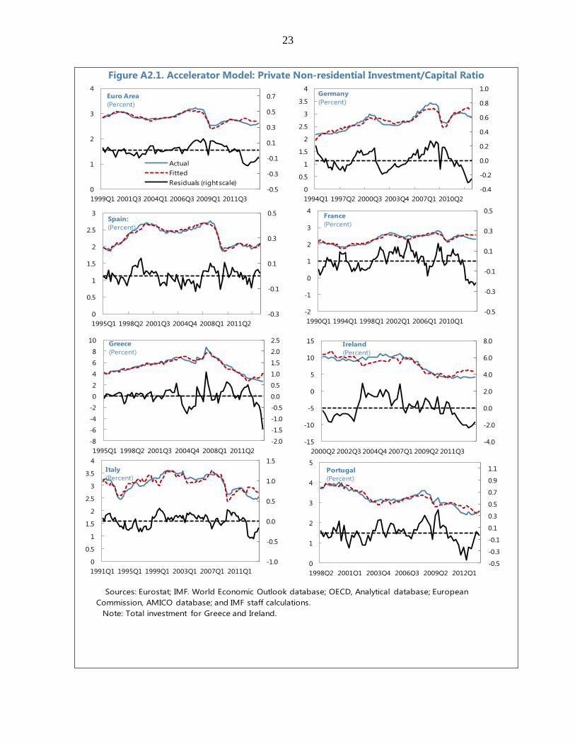
The accelerator model captures broad trends in investment, but also suggests sizeable
underinvestment (a level lower than the predicted value) for the countries considered for the
duration of the euro area debt crisis (2010Q2– 2013Q4), with the exception of Spain. The
model explains the variation in investment in Spain relatively well (text charts, and Figure
A2.1). For most countries, underinvestment becomes smaller towards the end of the sample.
However, the model does not seem to adequately explain the behavior of total investment in
Greece and Ireland.
Source: IMF staff estimates.
As robustness checks, we use different investment measures and methods to control for serial
correlation. We also consider different measures of machinery and equipment investment in
Ireland and Germany (with data up to 2013Q4). For both cases, the results are broadly the
same. Similarly, the main conclusions remain intact with Prais-Winsten estimates—an
alternative approach to address the residual auto-correlation—but the statistical significance
of the lagged terms declines for Ireland and Portugal.
B. Neoclassical Model
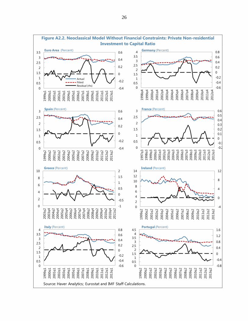
Because output developments cannot fully explain the decline in investment after the crisis,
we explore whether changes in the desired capital stock are better proxied by a measure
adjusted for the real cost of capital. The neoclassical model can be derived from equation (1),
similarly to the accelerator model, letting In theory, is expected to be positive.
As credit rationing cannot be fully captured by the real cost of capital estimates, the baseline
specification is augmented by a proxy for credit rationing (based on a question on financial
constraints from the European Commission’s consumer and business survey).
7 Given data availability, we also use lags up to 12 and report Newey-West standard errors. Oliner at. al., 1995 and Lee and
Rabanal, 2010 use similar lag lengths.
-0.3
-0.2
-0.1
0.0
0.1
0.2
0.3
0.4
0.5
0
1
2
3
4
1999Q1 2001Q3 2004Q1 2006Q3 2009Q1 2011Q3
Actual
Fitted
Residuals
Euro Area
(Percent)
-0.2
0.0
0.2
0.4
0
0.5
1
1.5
2
2.5
3
1995Q1 1998Q2 2001Q3 2004Q4 2008Q1 2011Q2
Spain:
(Percent)

11
where It refers to investment, Kt refers to capital stock, and fct refers to financial constraints.
Both nominal and real costs of capital are elevated for the stressed countries (See Appendix 1
for the definition of the cost of capital, and text charts). While reduced policy rates have
translated into lower borrowing costs and therefore a lower real cost of capital in the core
countries, borrowing costs have remained elevated in the stressed countries—a sign of
continued financial fragmentation. Keeping everything else constant, a higher real cost of
capital implies a lower level of desired capital stock and therefore a lower level of desired
investment.
Source: Eurostat; Haver Analytics; and IMF staff calculations.
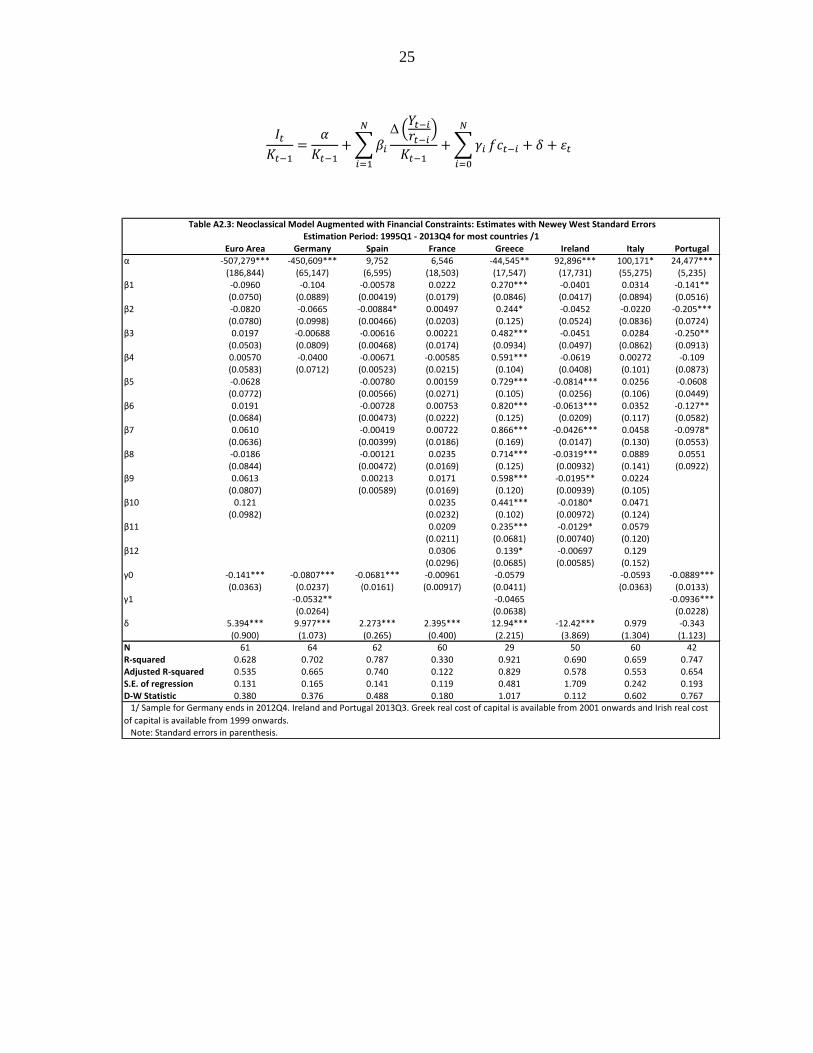
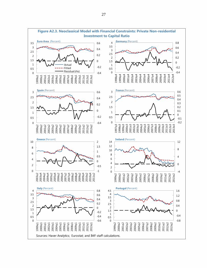
Similar to the accelerator model, the baseline neoclassical investment model suggests
significant underinvestment over the duration of the European debt crisis with the exception
of Spain (Table A2.3 and Figure A2.3).8 However, the coefficients on lagged desired changes
in capital stock (proxied by a function of output and real cost of capital) are generally not
statistically significant or positive, with the exception of Greece. A similar result has been
found by Oliner et.al (1995). In the augmented model, contemporary and lagged financial
constraints have significant negative effects on investment in the euro area as a whole, as
well as in Germany, Spain and Portugal. The gap between the actual and fitted investment in
the euro area and Italy closes towards the end of the estimation period (see text charts).
8 Similar to the accelerator model, the baseline residuals are serially correlated.
Source: IMF staff estimates
-0.4
-0.2
0
0.2
0.4
0.6
0
0.5
1
1.5
2
2.5
3
3.5
1999q
1
2000q
1
2001q
1
2002q
1
2003q
1
2004q
1
2005q
1
2006q
1
2007q
1
2008q
1
2009q
1
2010q
1
2011q
1
2012q
1
2013q
1
Actual
Fitted
Residual (rhs)
Euro Area (Percent)
-0.6
-0.4
-0.2
0
0.2
0.4
0.6
0.8
0
1
2
3
4
1999q
1
2000q
1
2001q
1
2002q
1
2003q
1
2004q
1
2005q
1
2006q
1
2007q
1
2008q
1
2009q
1
2010q
1
2011q
1
2012q
1
2013q
1
Actual
Fitted
Residual (rhs)
Italy (Percent)
1
3
5
7
9
11
1
3
5
7
9
11
Dec-
06
Jun-0
7
Dec-
07
Jun-0
8
Dec-
08
Jun-0
9
Dec-
09
Jun-1
0
Dec-
10
Jun-1
1
Dec-
11
Jun-1
2
Dec-
12
Jun-1
3
Dec-
13
Nominal Cost of Capital, percentage points
Euro Area SpainFrance GreeceIreland ItalyGermany Portugal
0
2
4
6
8
10
12
14
0
2
4
6
8
10
12
14
Dec-0
6
Jun
-07
Dec-0
7
Jun
-08
Dec-0
8
Jun
-09
Dec-0
9
Jun
-10
Dec-1
0
Jun
-11
Dec-1
1
Jun
-12
Dec-1
2
Jun
-13
Dec-1
3
Real Cost of Capital, percentage points
Euro Area Spain France
Italy Germany Portugal
12
These conclusions are qualitatively robust to alternate lag selection strategies, a measure of
the real cost of capital that is focused on debt financing only, and using narrower proxies for
non-residential investment for Germany and Ireland.9 To test whether the crisis has changed
the investment dynamics, an intercept and interaction dummies are added to the specification.
The intercept terms are generally significant, while the results are mixed for the interaction
terms.10
C. Accelerator + Model: Exploring Other Determinants of Investment
Beyond output dynamics and the real cost of capital, credit risk (through high corporate
leverage and corporate bond spreads), uncertainty, and cash flow may be important in
determining investment in line with earlier literature (Philippon 2009; Lee and Rabanal
2010). In this section, we augment the accelerator model with additional variables that can
explain euro area investment. Given the dominance of bank-based financing in Europe, to
control for differences in bank loan conditions across euro area countries, we use the real
lending rate for non-financial corporations (NFCs).11 To measure uncertainty, the paper uses
an economic policy uncertainty index, which is a weighted average of Consensus Economics
forecaster dispersion data and an index based on newspaper articles (Baker, Bloom, and
Davis 2013)12. While this measure captures overall policy uncertainty, it may not reflect firm
and sector specific risks and other types of uncertainty.13 In addition, we control for corporate
leverage and firms’ cash flow (Lee and Rabanal, 2010; REO APD, 2014). Leverage is
expected to be negatively correlated with investment in countries with high corporate
leverage and facing financing constraints. 14Accordingly, the ratio of private non-residential
investment to total capital stock is modeled as a function of overall real lending rates to
NFCs, corporate bond spreads, uncertainty, corporate leverage, and cash flow. Similar to the
neoclassical model, we also control for financial constraints to account for possible credit
rationing.15
9 We have experimented with allowing up to 12 lags in every model. 10 Out-of-sample projections also imply underinvestment. For all countries, one-step-ahead forecasts from 2008Q3 onward
produce projected investment levels that are above realized investment levels, particularly during the second phase of the
crisis. In the case of Germany, interestingly, during the first phase of the crisis, the decline in projected investment was
deeper than the actual decline. This has reversed during the second phase of the crisis. This pattern could reflect the
differences in the nature of shocks during the global crisis (2008–2010) and the European sovereign debt crisis (after 2010). 11 Estimations with the real policy rate produce very similar results. 12 Starting from April 2014, this index uses only the index based on news items. Our regressions stop at 2013Q4, and
therefore do not use this index. 13 A forthcoming paper focuses on firm specific and overall stock market volatility using firm level data. 14 If financing is not a problem and leverage is initially low, an increase in leverage could be positively correlated with
investment, particularly prior to the crisis. 15 The number of output change lags included is determined country-by-country on the basis of the Akaike information
criterion.

13
The additional variables (real lending rates, corporate bond spreads, uncertainty, corporate
leverage and cash flow) have significant effects on investment. Omitted variable tests show
that these factors are jointly significant in modeling investment both at the country and at the
euro area level (Table A2.5).16
High uncertainty is associated with weak investment, particularly in stressed
countries. Uncertainty reduces investment in the majority of the countries in the
sample (Spain, Italy, Greece, and Ireland) and in the euro area as a whole. A one
standard deviation increase in the uncertainty index reduces investment to capital
ratio by 0.03-0.1.
Corporate leverage is negatively correlated with investment in Portugal, Italy, and
France. These results are robust to using alternative definitions of firm leverage. In
these countries, one percentage point increase in the leverage ratio would reduce
investment to capital ratio by about 0.01–0.04 percentage points.
Financial constraints are negatively associated with investment for Italy and
Portugal.
Cash flow is found to be statistically significant and with the correct sign for Spain
and Germany. For Portugal the coefficient has the reverse sign (with weaker
statistical significance). Using a different cash flow-to-sales measure that gives a
larger weight to bigger corporations (market-capital weighted average) yields
similarly mixed results.
Corporate bond spreads are statistically significant for Ireland, Spain and, to a lesser
degree, Germany.
Real lending rates are either insignificant or their coefficients are wrongly signed for
most of the sample. The real lending rates significant and have the expected negative
correlation only for Italy. While the coefficients for the euro area, Germany and Spain
are statistically significant, they have the reverse sign—a common finding in the
literature (Caballero, 1999; Sharpe and Suarez, 2014).17 As this could reflect
difficulties in identifying credit demand and supply, we run a separate regression
including corporate bond spreads, the real rate and cash flow (representing supply
factors) as well as an instrumental variable based on GDP growth, uncertainty,
16 The omitted variable tests – for the euro area as well as the individual countries – take the restricted model with the
investment-to-total capital stock ratio as a function of only output changes and financial constraints as the starting point.
They then consider whether augmenting the model by uncertainty and leverage or by all additional factors increases the
explanatory power of the model, using F- and likelihood ratio tests of the null hypothesis that the coefficients of the added
variables are equal to zero. 17 The results remain basically unchanged when substituting with other lending rate variables such as the change in the real
lending rate, adding the real rate to the model as a separate variable, or interacting the real lending rate variable with a crisis
dummy to distinguish between boom and bust episodes.

14
-0.3
-0.2
-0.1
0.0
0.1
0.2
0.3
0.0
0.5
1.0
1.5
2.0
2.5
3.0
3.5
4.0
1999Q
1
2000Q
1
2001Q
1
2002Q
1
2003Q
1
2004Q
1
2005Q
1
2006Q
1
2007Q
1
2008Q
1
2009Q
1
2010Q
1
2011Q
1
2012Q
1
2013Q
1
Italy
Actual
Fitted
Residual (RHS)-0.3
-0.2
-0.1
0.0
0.1
0.2
0.3
0.0
0.5
1.0
1.5
2.0
2.5
3.0
3.5
1999Q
1
2000Q
1
2001Q
1
2002Q
1
2003Q
1
2004Q
1
2005Q
1
2006Q
1
2007Q
1
2008Q
1
2009Q
1
2010Q
1
2011Q
1
2012Q
1
2013Q
1
Euro Area
Actual
Fitted
Residual (RHS)
leverage and real lending rates to proxy demand factors. However, real rates are still
positively correlated with investment, suggesting that the regression is still picking up
the response of the policy rate to economic cycle.
Overall, the model seems to work better for stressed countries, in particular for Italy and
Spain, and to a lesser extent for Portugal and the euro area as a whole (Table A2.4 and Figure
A2.4).18 It performs comparatively poorly for Germany and France.19
Particularly for
countries with good fit, this model reduces the underinvestment observed in earlier models
for the post-crisis period substantially (see text charts).
Using the estimated coefficients from the Accelerator + model, we can separate the
contributions of output changes and all remaining factors to the evolution of investment
(Figure A2.5). For the euro area, output explains a large share of the weak investment from
2008 onwards, but the combined effect of uncertainty, corporate leverage and other
remaining factors also explain a share. For Spain, weak output explains almost all the decline
in investment during the crisis, but for Italy and Ireland, the additional factors were the main
drag on investment.
Additional robustness checks do not alter our findings. For example, using alternative
investment series for machinery and equipment investment in Ireland and Germany (with
data up to 2013Q4) produces broadly similar results. The results are also robust to using
alternative estimation techniques to correct for residual autocorrelation. Employing a
Cochrane-Orcutt estimation method instead of the Newey-West estimator, the signs of the
coefficients remain the same, though their size and significance level differ slightly from the
results reported above.
The paper also explored the Tobin’s Q model, but the model did not perform well in
explaining investment, possibly reflecting data measurement issues at the aggregate level.
18 For Portugal, after controlling for other factors some output coefficients turn negative. This could potentially reflect
omitted variable bias, stemming from the EU structural funds, which have played an important role in investment in
Portugal. 19 Pérez Ruiz (2014) uses a broader set of determinants to explain the level of business investment in France. The model
provides a good fit for France.
Source: IMF staff estimates
15
-12.0
-10.0
-8.0
-6.0
-4.0
-2.0
0.0
2.0
Germany Spain France Italy Portugal Euro Area
Unexplained Investment Shortfall
(Since 2010Q2, in percent of GDP)
Accelerator Model
Neoclassical Model
Accelerator + Model
Several definitions of Tobin’s Q (for NFCs) were considered: i) quarterly series that are
interpolated from annual Tobin’s Q (Woldscope, Corporate Vulnerability Unit); ii) price-to-
book ratio; iii) stock prices deflated by GDP deflator. In addition, the model controls for firm
leverage (debt-to-asset ratio) and cash-flow. Among the Tobin’s Q proxies used, only price-
to-book ratio appears to be significant in a few specifications for Germany, France, and
Portugal. Controlling for endogeneity (by two-stage least squares) and running the
regressions for the pre-crisis period, the significance of the results increases somewhat: price-
to-book ratio and leverage are significant and correctly signed for Germany, Greece,
Portugal, and the euro area. Overall, however, model performance remains weak. This could
reflect measurement issues with aggregate data, lack of quarterly series, and the dominance
of unlisted companies (mainly SMEs) in some countries. These results are available upon
request.
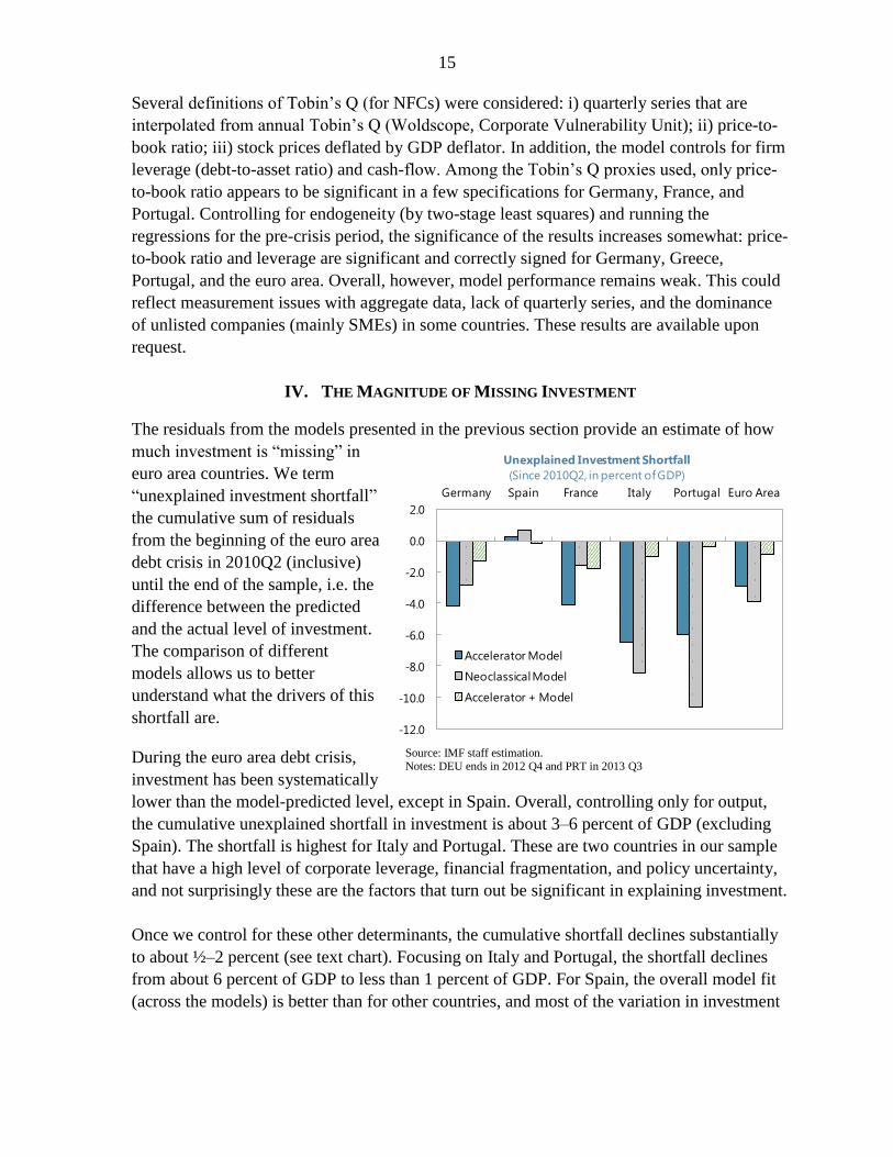
IV. THE MAGNITUDE OF MISSING INVESTMENT
The residuals from the models presented in the previous section provide an estimate of how
much investment is “missing” in
euro area countries. We term
“unexplained investment shortfall”
the cumulative sum of residuals
from the beginning of the euro area
debt crisis in 2010Q2 (inclusive)
until the end of the sample, i.e. the
difference between the predicted
and the actual level of investment.
The comparison of different
models allows us to better
understand what the drivers of this
shortfall are.
During the euro area debt crisis,
investment has been systematically
lower than the model-predicted level, except in Spain. Overall, controlling only for output,
the cumulative unexplained shortfall in investment is about 3–6 percent of GDP (excluding
Spain). The shortfall is highest for Italy and Portugal. These are two countries in our sample
that have a high level of corporate leverage, financial fragmentation, and policy uncertainty,
and not surprisingly these are the factors that turn out be significant in explaining investment.
Once we control for these other determinants, the cumulative shortfall declines substantially
to about ½–2 percent (see text chart). Focusing on Italy and Portugal, the shortfall declines
from about 6 percent of GDP to less than 1 percent of GDP. For Spain, the overall model fit
(across the models) is better than for other countries, and most of the variation in investment
Source: IMF staff estimation. Notes: DEU ends in 2012 Q4 and PRT in 2013 Q3

16
is explained with all the models. As a result, the missing investment for Spain is around zero
across the models.
V. CONCLUSION
Weak investment across the euro area has been driven by a combination of factors. Empirical
evidence suggests that output dynamics can explain the broad trends in investment, including
a part of its collapse after the financial crisis. In particular, output can explain almost all of
the movement in investment in Spain. In other countries, however, private non-residential
investment has been lower than implied by output developments since the onset of the
European debt crisis.
In addition to output dynamics, financial constraints affect investment, particularly for Italy,
Portugal, and Spain. The neoclassical model that seeks to proxy desired capital stock with a
measure based on the real cost of capital generally does not produce significant results,
except for Greece. Nevertheless, investment continues to remain below its model implied
value for most of the countries.
High uncertainty and corporate sector leverage are additional impediments to investment,
particularly for some of the stressed countries. These factors explain a big portion of the
decline in investment that was not explained by output changes and real cost of capital.
Based on these results, investment is expected to pick up as the recovery strengthens and
uncertainty declines. The recovery in the euro area is ultimately grounded in complementary
policy actions at both at the national and euro area levels. Demand support, balance sheet
repair, completion of the banking union, and structural reforms are needed to further
strengthen the euro area economy and reduce uncertainty (Euro Area Policies: 2014 Article
Consultation Staff Report, IMF, 2014b). Corporate debt-to-equity remains elevated in some
stressed countries, and the deleveraging process is still at an early stage. At the same time,
firms’ access to capital needs to improve in stressed countries to support investment. A
sustained recovery in investment will require dealing with both the corporate debt overhang
and financial fragmentation.
Building on the evidence from aggregate data, future work will focus on firm-level
investment, particularly for SMEs. Firm-level analysis will supplement macro-level
regressions and differentiate better investment patterns of large and small corporations. It
will also better capture the impact of other firm-specific variables, such as cash flow,
leverage, and Tobin’s Q.

17
References
Baker, Scott; Bloom, Nicholas; Davis, Steven, 2013, “Measuring Economic Policy
Uncertainty”, Chicago Booth Research Paper No. 13-02.
Baum, Christopher; Caglayan, Mustafa; and Talavera, Oleksandr, 2010, “On the investment
sensitivity of debt under uncertainty”, Economics Letters, Vol. 106, pp. 25–27.
Bloom, Nick, 2009, “The Impact of Uncertainty Shocks,” Econometrica, Vol. 77, No. 3, pp.
623–85.
Bloom, Nick; Bond, Stephen; and Van Reenen, John, 2007, “Uncertainty and Investment
Dynamics”, Review of Economic Studies, Vol. 74, pp. 391-415.
———, Max Floetotto, and Nir Jamovich, 2009, “Really Uncertain Business Cycles”
(unpublished; Palo Alto, California: Stanford University).
Bond, Stephen; Elston, Julie Ann; Mairesse, Jacques; and Mulkay, Benoit, 2003, “Financial
Factors and Investment in Belgium, France, Germany, and the United Kingdom: A
Comparison Using Company Panel Data” The Review of Economics and Statistics,
Vol. 85(1), pp. 153–165.
Caballero, Ricardo, 1994, “Small Sample Bias and Adjustment Costs,” Review of Economics
and Statistics, Vol. 76, No. 1, pp. 52–58.
Caballero, Ricardo J., 1999, Aggregate Investment, in John B. Taylor and Michael
Woodford, eds., Handbook of macroeconomics, Vol 1B, Amsterdam: Elsevier.
Clark, J.M., 1917, “Business Acceleration and the Law of Demand: A Technical Factor in
Economic Cycles,” Journal of Political Economy, Vol. 25, pp. 217–35.
Dixit, Avinash and Robert Pindyck, 1994, “Investment Under Uncertainty” (Princeton, NJ:
Princeton University Press).
European Investment Bank (EIB), 2013, Investment and Investment Finance in Europe,
http://www.eib.org/infocentre/publications/all/investment-and-investment-finance-in-
europe.htm
Hayashi, Fumio, 1982, “Tobin’s Marginal q and Average q: A Neoclassical Interpretation,”
Econometrica, Vol. 50, pp. 213–24.
IMF, Baltic Cluster Report, 2014 Cluster Consultation, Selected Issues, IMF Country Report
No. 14/117.

18
IMF, Euro Area Policies: 2014 Article IV Consultation-Staff Report, IMF Country Report
No. 14/198.
IMF, Euro Area Policies: Selected Issues; IMF, Country Report No. 14/199; June 26, 2014
Jorgenson, D.W., 1971, “Econometric Studies of Investment Behavior: A Survey”, Journal of
Economic Literature, Vol. 9, pp. 1111–47.
Laeven, Luc and Fabián Valencia, 2012, “Systemic Banking Crises Database: An Update”,
IMF Working Paper 12/163 (Washington: International Monetary Fund).
Lee, Jaewoo, and Pau Rabanal, 2010, “Forecasting U.S. Investment”, IMF Working Paper
10/246 (Washington: International Monetary Fund).
Mizen, Paul and Vermeulen, Philip, 2005,”Corporate Investment and Cash-Flow Sensitivity:
What Drives the Relationship”, ECB Working Paper Series, No. 485 / May 2005.
Oliner, Stephen, Glenn Rudebusch, and Daniel Sichel, 1995 “New and Old Models of
Business Investment: A Comparison of Forecasting Performance,” Journal of Money,
Credit, and Banking, Vol. 27, No. 3, pp. 806–26.
Pérez Ruiz, Esther, 2014, “The Drivers of Business Investment in France: Reasons for
Recent Weakness”, France Selected Issues, Country Report No. 14/183.
Phillippon, Thomas, 2009, “The Bond Market’s Q,” Quarterly Journal of Economics, Vol.
124, No. 3, pp. 1011–56.
Pina, Alvaro and Abreu, Ildeberta, 2012, “Portugal: Rebalancing the Economy and Returning
to Growth Through Job Creation and Better Capital Allocation”, OECD WP 994.
Regional Economic Outlook (REO): Asia and Pacific, April 2014, “Sustaining the
Momentum: Vigilance and Reforms”, Chapter 2: “Corporate Leverage in Asia: A
Fault Line?”, (Washington: International Monetary Fund).
Sharpe, Steven A. and Gustavo A. Suarez, 2014, “The Insensitivity of Investment to Interest
Rates: Evidence from a Survey of CFOs”, Finance and Economics Discussion Series,
Federal Reserve Board, Washington D.C.
Tobin, James, 1969, “A General Equilibrium Approach to Monetary Theory,” Journal of
Money, Credit and Banking, Vol. 1, pp. 15–29.
World Economic Outlook (WEO), April 2014, “Recovery Strengthens, Remains Uneven”:
Chapter 3: “Perspectives on Global Real Interest Rates”, (Washington: International
Monetary Fund).

19
APPENDIX 1. DATA DEFINITIONS AND SOURCES
Real investment. Investment data are taken from the Eurostat with the exception of Greece and
Ireland, where World Economic Outlook (WEO) data for total investment is used. Private non-
residential investment is the sum of investment in transport and other machinery and equipment,
cultivated assets, and intangible fixed assets. Left panel of the first text figure uses the following
sources:
Greece: Gross capital formation, (NSA, millions of chained 2005 euro); source – ELSTAT;
Haver code - N174NCC@G10. Ireland: Gross fixed capital formation (SA, millions of chained
2011 euro); source – CSOI; Haver code - S178NFC@G10. Spain: Gross capital formation
(SA/WDA, millions of chained 2008 euro); source – INE; Haver code - S184NFBC@G10.
Portugal: Gross capital formation (SA, millions of chained 2006 euro); source – INE; Haver code
- S182NFBC@G10. Italy: Gross fixed investment (SA/WDA, millions of chained 2005 euro);
source – ISTAT; Haver code - S136NFC@G10. Euro Area: Gross capital formation (SA/WDA,
millions of chained 2005 euro); source – Eurostat; Haver code - S025NFBC@G10. United
Kingdom: Gross fixed capital formation (SA, millions of chained 2010 pounds); source – ONS;
Haver code - S112NFC@G10. France: Gross fixed capital formation (SWDA, millions of
Chained 2010 euro); source – INSEE; Haver code - FRSNFIC@FRANCE. United States: gross
capital formation (SA, billions of chained 2009 dollars); source – BEA; Haver code -
S111NFBC@G10. Germany: Gross capital formation (SA/WDA, billions of chained 2005 euro);
source – Bundesbank; Haver code - S134NFBC@G10.
Capital stock series are from AMECO database—the annual series were linearly interpolated so
that the stock of capital in the last quarter would match the corresponding annual figure.
Alternative measures of capital stock were also calculated using perpetual inventory method. The
initial capital stock values from the AMECO capital stock were scaled by applying appropriate
investment subcomponent ratios. Depreciation rates are assumed constant and equal to average
rates implied by the AMECO series.
Real GDP on quarterly basis was obtained from the WEO database.
Real cost of capital. The correct measure of the cost of capital depends on the structure of
financing of the firm. The flow of funds data suggests that liabilities of non-financial
corporations consist primarily of loans and equity with the share of bond financing being less
than 10 percent in most periods and countries. The following formula is used for the real cost of
capital:
where , and , are the amounts of bank loans, bonds (securities other than shares), and
equity in the liabilities of non-financial corporations. For the nominal costs of different kind of
capital we use MFI lending rates in a given country for new business at all maturities, , for
bank loan liabilities; yield on the euro area wide corporate bond index, , for bond liabilities; and
the yield on 10 year government bond to price equity liabilities.20
20 We have experimented with alternative approaches to price equity capital – such as variations on the dividend growth
model; however, they tend to produce counterintuitive implications for the ranking of the cost of capital across different
countries. Using a 10-year government bond establishes a sensible lower bound for the cost of equity and, assuming that the
(continued…)
20
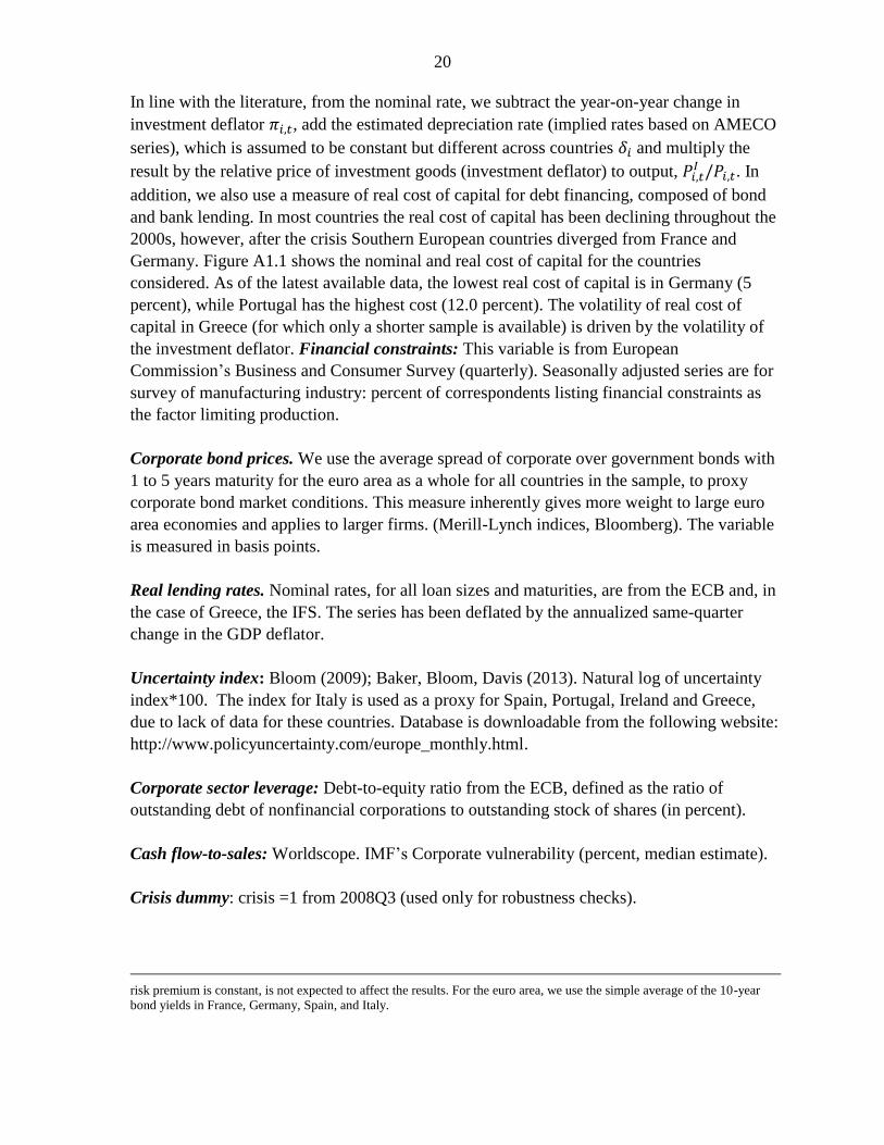
In line with the literature, from the nominal rate, we subtract the year-on-year change in
investment deflator , add the estimated depreciation rate (implied rates based on AMECO
series), which is assumed to be constant but different across countries and multiply the
result by the relative price of investment goods (investment deflator) to output, . In
addition, we also use a measure of real cost of capital for debt financing, composed of bond
and bank lending. In most countries the real cost of capital has been declining throughout the
2000s, however, after the crisis Southern European countries diverged from France and
Germany. Figure A1.1 shows the nominal and real cost of capital for the countries
considered. As of the latest available data, the lowest real cost of capital is in Germany (5
percent), while Portugal has the highest cost (12.0 percent). The volatility of real cost of
capital in Greece (for which only a shorter sample is available) is driven by the volatility of
the investment deflator. Financial constraints: This variable is from European
Commission’s Business and Consumer Survey (quarterly). Seasonally adjusted series are for
survey of manufacturing industry: percent of correspondents listing financial constraints as
the factor limiting production.
Corporate bond prices. We use the average spread of corporate over government bonds with
1 to 5 years maturity for the euro area as a whole for all countries in the sample, to proxy
corporate bond market conditions. This measure inherently gives more weight to large euro
area economies and applies to larger firms. (Merill-Lynch indices, Bloomberg). The variable
is measured in basis points.
Real lending rates. Nominal rates, for all loan sizes and maturities, are from the ECB and, in
the case of Greece, the IFS. The series has been deflated by the annualized same-quarter
change in the GDP deflator.
Uncertainty index: Bloom (2009); Baker, Bloom, Davis (2013). Natural log of uncertainty
index*100. The index for Italy is used as a proxy for Spain, Portugal, Ireland and Greece,
due to lack of data for these countries. Database is downloadable from the following website:
http://www.policyuncertainty.com/europe_monthly.html.
Corporate sector leverage: Debt-to-equity ratio from the ECB, defined as the ratio of
outstanding debt of nonfinancial corporations to outstanding stock of shares (in percent).
Cash flow-to-sales: Worldscope. IMF’s Corporate vulnerability (percent, median estimate).
Crisis dummy: crisis =1 from 2008Q3 (used only for robustness checks).
risk premium is constant, is not expected to affect the results. For the euro area, we use the simple average of the 10-year
bond yields in France, Germany, Spain, and Italy.

21
Figure A1.1. Cost of Capital Calculations
Figure 1. Cost of Capital Calculations
Source: Haver Analytics; and IMF staff estimates.
0
2
4
6
8
10
12
14
19954
19971
19982
19993
20004
20021
20032
20043
20054
20071
20082
20093
20104
20121
20132
Germany: Cost of Capital, percentage points
Real
Nominal
0
2
4
6
8
10
12
14
19954
19971
19982
19993
20004
20021
20032
20043
20054
20071
20082
20093
20104
20121
20132
Spain: Cost of Capital, percentage points
Real
Nominal
0
2
4
6
8
10
12
19954
19971
19982
19993
20004
20021
20032
20043
20054
20071
20082
20093
20104
20121
20132
France: Cost of Capital, percentage points
Real
Nominal
0
2
4
6
8
10
12
14
19954
19971
19982
19993
20004
20021
20032
20043
20054
20071
20082
20093
20104
20121
20132
Greece: Cost of Capital, percentage points
Real
Nominal
-5
0
5
10
15
20
19
95
4
19
97
1
19982
19993
20004
20021
20032
20
04
3
20
05
4
20
07
1
20
08
2
20
09
3
20104
20121
20132
Ireland: Cost of Capital, percentage points
Real
Nominal
0
2
4
6
8
10
12
14
19954
19971
19982
19993
20004
20021
20032
20043
20054
20071
20082
20093
20104
20121
20132
Italy: Cost of Capital, percentage points
Real
Nominal
0
2
4
6
8
10
12
14
16
19954
19971
19982
19993
20004
20021
20032
20043
20054
20071
20082
20093
20104
20121
20132
Portugal: Cost of Capital, percentage points
Real Nominal
0
2
4
6
8
10
12
14
19954
19971
19982
19993
20004
20021
20032
20043
20054
20071
20082
20093
20104
20121
20132
Euro Area: Cost of Capital, percentage points
Real
Nominal

22
APPENDIX 2. RESULTS
RESULTS OF THE ACCELERATOR MODEL21
11 1 1
Nt t i
i t
it t t
I Ye
K K K
21 Results are in percent terms.
Table A2.1 Accelerator Model - Total Investments (Newey-West HAC standard error estimates)
Euro Area Germany Spain France Greece Ireland Italy Portugal
α -200700 ** -222248 *** -22311 *** -90732 *** -37403 *** -15327 -57655 *** -3756(97242.82) (23056.6) (1592.14) (7255.75) (2735.32) (13273.16) (11991.01) (2851.86)
β1 0.32 *** 0.21 *** 0.41 *** 0.26 *** 0.38 ** 0.75 ** 0.47 *** 0.29 ***(0.06) (0.06) (0.09) (0.06) (0.17) (0.28) (0.08) (0.08)
β2 0.21 ** 0.23 *** 0.49 *** 0.23 *** 0.70 *** 0.99 ** 0.39 *** 0.26 **(0.1) (0.07) (0.06) (0.05) (0.15) (0.42) (0.09) (0.1)
β3 0.25 *** 0.25 *** 0.23 *** 0.23 *** 1.10 *** 0.92 ** 0.37 *** 0.26 ***(0.06) (0.06) (0.07) (0.05) (0.1) (0.38) (0.07) (0.06)
β4 0.22 *** 0.18 *** -0.05 0.20 *** 0.71 *** 0.76 ** 0.19 ** 0.24 ***(0.07) (0.04) (0.08) (0.05) (0.12) (0.29) (0.08) (0.07)
β5 0.13 * 0.13 *** 0.12 * 0.20 *** 1.04 *** 0.37 0.27 *** 0.21 **(0.07) (0.04) (0.07) (0.05) (0.12) (0.35) (0.09) (0.08)
β6 0.16 *** 0.10 ** 0.39 *** 0.17 *** 1.12 *** 0.30 0.18 *** 0.19 **(0.05) (0.04) (0.06) (0.06) (0.16) (0.39) (0.07) (0.08)
β7 0.17 ** 0.07 0.09 0.09 * 0.82 *** 0.28 0.28 *** 0.22 ***(0.07) (0.05) (0.06) (0.06) (0.18) (0.33) (0.07) (0.07)
β8 0.06 0.09 * 0.00 0.12 ** 0.57 ** 0.24 *** 0.10(0.04) (0.05) (0.05) (0.05) (0.25) (0.07) (0.07)
β9 0.10 ** 0.12 ** 0.05 0.11 ** 0.55 0.09 0.16 **(0.05) (0.06) (0.04) (0.05) (0.34) (0.07) (0.08)
β10 0.09 * 0.07 0.15 *** 0.10 ** 0.71 * 0.18 *** 0.16 *(0.05) (0.05) (0.03) (0.05) (0.39) (0.06) (0.09)
β11 0.05 0.10 * 0.06 * 0.08 1.04 *** 0.26 *** 0.17 *(0.04) (0.05) (0.03) (0.05) (0.35) (0.07) (0.09)
β12 0.18 *** 0.20 *** 0.75 ** 0.38 *** 0.16 *(0.05) (0.06) (0.3) (0.08) (0.08)
δ 3.43 *** 5.99 *** 2.76 *** 3.98 *** 10.65 *** 8.92 *** 4.29 *** 3.81 ***(0.38) (0.35) (0.05) (0.16) (0.48) (2.75) (0.3) (0.66)
N 60 76 76 96 76 54 92 62Adjusted R-squared 0.79 0.82 0.95 0.86 0.92 0.66 0.75 0.82D-W Statistic 0.50 0.38 0.99 0.33 0.69 0.50 0.35 0.80S.E. of regression 0.09 0.14 0.06 0.10 0.39 1.52 0.18 0.180.09 0.14 0.06 0.10 0.39 1.52 0.18 0.18
Notes: * - significant at 10 percent; ** - significant at 5 percent; *** - significant at 1 percent. EA sample includes 1991Q1 - 2013Q4; Germany: 1994Q1-2012Q4;Spain and Greece: 1995Q1 - 2013Q4; France: 1990Q1 - 2013Q4; Ireland: 2000Q2 - 2013Q3; Italy: 1991Q1 - 2013Q4; Portugal: 1998Q2 - 2013Q3. Standard errors in parenthesis.
23
Figure A2.1. Accelerator Model: Private Non-residential Investment/Capital Ratio
Figure 1. Accelerator Model: Private Non-residential Investment/Capital Ratio
Sources: Eurostat; IMF. World Economic Outlook database; OECD, Analytical database; European
Commission, AMICO database; and IMF staff calculations.
Note: Total investment for Greece and Ireland.
-0.4
-0.2
0.0
0.2
0.4
0.6
0.8
1.0
0
0.5
1
1.5
2
2.5
3
3.5
4
1994Q1 1997Q2 2000Q3 2003Q4 2007Q1 2010Q2
Germany
(Percent)
-0.3
-0.1
0.1
0.3
0.5
0
0.5
1
1.5
2
2.5
3
1995Q1 1998Q2 2001Q3 2004Q4 2008Q1 2011Q2
Spain:
(Percent)
-0.5
-0.3
-0.1
0.1
0.3
0.5
-2
-1
0
1
2
3
4
1990Q1 1994Q1 1998Q1 2002Q1 2006Q1 2010Q1
France
(Percent)
-2.0
-1.5
-1.0
-0.5
0.0
0.5
1.0
1.5
2.0
2.5
-8
-6
-4
-2
0
2
4
6
8
10
1995Q1 1998Q2 2001Q3 2004Q4 2008Q1 2011Q2
Greece
(Percent)
-4.0
-2.0
0.0
2.0
4.0
6.0
8.0
-15
-10
-5
0
5
10
15
2000Q2 2002Q3 2004Q4 2007Q1 2009Q2 2011Q3
Ireland
(Percent)
-1.0
-0.5
0.0
0.5
1.0
1.5
0
0.5
1
1.5
2
2.5
3
3.5
4
1991Q1 1995Q1 1999Q1 2003Q1 2007Q1 2011Q1
Italy
(Percent)
-0.5
-0.3
-0.1
0.1
0.3
0.5
0.7
0.9
1.1
0
1
2
3
4
5
1998Q2 2001Q1 2003Q4 2006Q3 2009Q2 2012Q1
Portugal
(Percent)
-0.5
-0.3
-0.1
0.1
0.3
0.5
0.7
0
1
2
3
4
1999Q1 2001Q3 2004Q1 2006Q3 2009Q1 2011Q3
Actual
Fitted
Residuals (right scale)
Euro Area
(Percent)

24
RESULTS OF THE NEOCLASSICAL MODEL
Euro Area Germany Spain France Greece Ireland Italy Portugalα 241,396** -205,726*** 34,672*** 22,430 -51,155*** 92,896*** 166,796*** 12,617***
(95,654) (49,825) (7,454) (13,375) (10,192) (17,731) (45,868) (1,816)β1 -0.142 -0.0623 -0.00878 0.0226 0.244*** -0.0401 -0.000238 0.00587
(0.101) (0.135) (0.0109) (0.0203) (0.0637) (0.0417) (0.0825) (0.0386)β2 -0.0927 -0.0766 -0.00998 0.00837 0.202** -0.0452 -0.0122 0.0201
(0.0942) (0.132) (0.0118) (0.0215) (0.0807) (0.0524) (0.0694) (0.0412)β3 -0.00225 -0.0339 -0.00900 0.00535 0.467*** -0.0451 0.0176 -0.0156
(0.0772) (0.122) (0.0120) (0.0193) (0.0610) (0.0497) (0.0788) (0.0492)β4 -0.0560 0.00871 -0.00996 -0.00782 0.600*** -0.0619 -0.0197 -0.0154
(0.0916) (0.0836) (0.0132) (0.0208) (0.0692) (0.0408) (0.0888) (0.0472)β5 -0.0952 -0.0102 0.00393 0.757*** -0.0814*** 0.00507 0.00611
(0.0937) (0.0133) (0.0267) (0.0788) (0.0256) (0.110) (0.0470)β6 0.0392 -0.00869 0.00895 0.909*** -0.0613*** 0.0202 -0.0262
(0.0837) (0.0121) (0.0222) (0.104) (0.0209) (0.113) (0.0567)β7 0.0710 -0.00514 0.00957 0.976*** -0.0426*** 0.0167 0.00711
(0.0707) (0.0108) (0.0195) (0.124) (0.0147) (0.132) (0.0620)β8 0.0184 -0.00168 0.0236 0.829*** -0.0319*** 0.0575 0.00266
(0.0921) (0.0112) (0.0180) (0.114) (0.00932) (0.140) (0.0599)β9 0.0756 0.00284 0.0169 0.704*** -0.0195** 0.0151
(0.0973) (0.0123) (0.0173) (0.0946) (0.00939) (0.119)β10 0.157 0.0277 0.511*** -0.0180* 0.00667
(0.124) (0.0224) (0.0876) (0.00972) (0.127)β11 0.0240 0.270*** -0.0129* 0.0365
(0.0230) (0.0613) (0.00740) (0.128)β12 0.0309 0.154** -0.00697 0.107
(0.0309) (0.0611) (0.00585) (0.159)δ 1.855*** 5.937*** 1.224*** 2.040*** 13.24*** -12.42*** -0.696 0.135
(0.394) (0.792) (0.268) (0.267) (1.505) (3.869) (1.044) (0.480)N 61 64 62 60 29 50 60 62R-squared 0.310 0.397 0.511 0.312 0.907 0.690 0.624 0.633Adjusted R-squared 0.155 0.345 0.415 0.118 0.827 0.578 0.517 0.570S.E. of regression 0.177 0.231 0.211 0.119 0.485 1.709 0.251 0.283D-W Statistic 0.234 0.184 0.182 0.231 0.862 0.281 0.156 0.150
Table A2.2: Neoclassical Model: Estimates with Newey West Standard ErrorsEstimation Period: 1995Q1 - 2013Q4 for most countries /1
1/ Sample for Germany ends in 2012Q4. Ireland and Portugal 2013Q3. Greek real cost of capital is available from 2001 onwards and Irish
real cost of capital is available from 1999 onwards. Note: Standard errors in parenthesis.
25
Euro Area Germany Spain France Greece Ireland Italy Portugalα -507,279*** -450,609*** 9,752 6,546 -44,545** 92,896*** 100,171* 24,477***
(186,844) (65,147) (6,595) (18,503) (17,547) (17,731) (55,275) (5,235)β1 -0.0960 -0.104 -0.00578 0.0222 0.270*** -0.0401 0.0314 -0.141**
(0.0750) (0.0889) (0.00419) (0.0179) (0.0846) (0.0417) (0.0894) (0.0516)β2 -0.0820 -0.0665 -0.00884* 0.00497 0.244* -0.0452 -0.0220 -0.205***
(0.0780) (0.0998) (0.00466) (0.0203) (0.125) (0.0524) (0.0836) (0.0724)β3 0.0197 -0.00688 -0.00616 0.00221 0.482*** -0.0451 0.0284 -0.250**
(0.0503) (0.0809) (0.00468) (0.0174) (0.0934) (0.0497) (0.0862) (0.0913)β4 0.00570 -0.0400 -0.00671 -0.00585 0.591*** -0.0619 0.00272 -0.109
(0.0583) (0.0712) (0.00523) (0.0215) (0.104) (0.0408) (0.101) (0.0873)β5 -0.0628 -0.00780 0.00159 0.729*** -0.0814*** 0.0256 -0.0608
(0.0772) (0.00566) (0.0271) (0.105) (0.0256) (0.106) (0.0449)β6 0.0191 -0.00728 0.00753 0.820*** -0.0613*** 0.0352 -0.127**
(0.0684) (0.00473) (0.0222) (0.125) (0.0209) (0.117) (0.0582)β7 0.0610 -0.00419 0.00722 0.866*** -0.0426*** 0.0458 -0.0978*
(0.0636) (0.00399) (0.0186) (0.169) (0.0147) (0.130) (0.0553)β8 -0.0186 -0.00121 0.0235 0.714*** -0.0319*** 0.0889 0.0551
(0.0844) (0.00472) (0.0169) (0.125) (0.00932) (0.141) (0.0922)β9 0.0613 0.00213 0.0171 0.598*** -0.0195** 0.0224
(0.0807) (0.00589) (0.0169) (0.120) (0.00939) (0.105)β10 0.121 0.0235 0.441*** -0.0180* 0.0471
(0.0982) (0.0232) (0.102) (0.00972) (0.124)β11 0.0209 0.235*** -0.0129* 0.0579
(0.0211) (0.0681) (0.00740) (0.120)β12 0.0306 0.139* -0.00697 0.129
(0.0296) (0.0685) (0.00585) (0.152)γ0 -0.141*** -0.0807*** -0.0681*** -0.00961 -0.0579 -0.0593 -0.0889***
(0.0363) (0.0237) (0.0161) (0.00917) (0.0411) (0.0363) (0.0133)γ1 -0.0532** -0.0465 -0.0936***
(0.0264) (0.0638) (0.0228)δ 5.394*** 9.977*** 2.273*** 2.395*** 12.94*** -12.42*** 0.979 -0.343
(0.900) (1.073) (0.265) (0.400) (2.215) (3.869) (1.304) (1.123)N 61 64 62 60 29 50 60 42R-squared 0.628 0.702 0.787 0.330 0.921 0.690 0.659 0.747Adjusted R-squared 0.535 0.665 0.740 0.122 0.829 0.578 0.553 0.654S.E. of regression 0.131 0.165 0.141 0.119 0.481 1.709 0.242 0.193D-W Statistic 0.380 0.376 0.488 0.180 1.017 0.112 0.602 0.767
Table A2.3: Neoclassical Model Augmented with Financial Constraints: Estimates with Newey West Standard ErrorsEstimation Period: 1995Q1 - 2013Q4 for most countries /1
1/ Sample for Germany ends in 2012Q4. Ireland and Portugal 2013Q3. Greek real cost of capital is available from 2001 onwards and Irish real cost
of capital is available from 1999 onwards. Note: Standard errors in parenthesis.
26
Source: Haver Analytics; Eurostat and IMF Staff Calculations.
-0.4
-0.2
0
0.2
0.4
0.6
0
0.5
1
1.5
2
2.5
3
3.5
1999q
1
2000q
1
2001q
1
2002q
1
2003q
1
2004q
1
2005q
1
2006q
1
2007q
1
2008q
1
2009q
1
2010q
1
2011q
1
2012q
1
2013q
1
Actual
Fitted
Residual (rhs)
Euro Area (Percent)
-0.6
-0.4
-0.2
0
0.2
0.4
0.6
0.8
0
0.5
1
1.5
2
2.5
3
3.5
4
1998q
4
1999q
4
2000q
4
2001q
4
2002q
4
2003q
4
2004q
4
2005q
4
2006q
4
2007q
4
2008q
4
2009q
4
2010q
4
2011q
4
2012q
4
Germany (Percent)
-0.4
-0.2
0
0.2
0.4
0.6
0
0.5
1
1.5
2
2.5
3
1999q
2
2000q
2
2001q
2
2002q
2
2003q
2
2004q
2
2005q
2
2006q
2
2007q
2
2008q
2
2009q
2
2010q
2
2011q
2
2012q
2
2013q
2Spain (Percent)
-0.2
-0.1
0
0.1
0.2
0.3
0.4
0.5
0.6
0
0.5
1
1.5
2
2.5
3
1997q
3
1998q
3
1999q
3
2000q
3
2001q
3
2002q
3
2003q
3
2004q
3
2005q
3
2006q
3
2007q
3
2008q
3
2009q
3
2010q
3
2011q
3
2012q
3
2013q
3
France (Percent)
-1
-0.5
0
0.5
1
1.5
2
0
2
4
6
8
10
2003q
2
2003q
4
2004q
2
2004q
4
2005q
2
2005q
4
2006q
2
2006q
4
2007q
2
2007q
4
2008q
2
2008q
4
2009q
2
2009q
4
2010q
2
2010q
4
2011q
2
Greece (Percent)
-4
0
4
8
12
0
2
4
6
8
10
12
14
1999q
2
2000q
2
2001q
2
2002q
2
2003q
2
2004q
2
2005q
2
2006q
2
2007q
2
2008q
2
2009q
2
2010q
2
2011q
2
2012q
2
2013q
2
Ireland (Percent)
-0.6
-0.4
-0.2
0
0.2
0.4
0.6
0.8
0
0.5
1
1.5
2
2.5
3
3.5
4
1999q
1
2000q
1
2001q
1
2002q
1
2003q
1
2004q
1
2005q
1
2006q
1
2007q
1
2008q
1
2009q
1
2010q
1
2011q
1
2012q
1
2013q
1
Italy (Percent)
-0.8
-0.4
0
0.4
0.8
1.2
1.6
0
0.5
1
1.5
2
2.5
3
3.5
4
4.5
1999q
2
2000q
2
2001q
2
2002q
2
2003q
2
2004q
2
2005q
2
2006q
2
2007q
2
2008q
2
2009q
2
2010q
2
2011q
2
2012q
2
2013q
2
Portugal (Percent)
Figure A2.2. Neoclassical Model Without Financial Constraints: Private Non-residential
Investment to Capital Ratio
27
Sources: Haver Analytics; Eurostat; and IMF staff calculations.
-0.4
-0.2
0
0.2
0.4
0.6
0
0.5
1
1.5
2
2.5
3
3.5
1999q
1
2000q
1
2001q
1
2002q
1
2003q
1
2004q
1
2005q
1
2006q
1
2007q
1
2008q
1
2009q
1
2010q
1
2011q
1
2012q
1
2013q
1
Actual
Fitted
Residual (rhs)
Euro Area (Percent)
-0.4
-0.2
0
0.2
0.4
0.6
0.8
0
0.5
1
1.5
2
2.5
3
3.5
4
1998q
4
1999q
4
2000q
4
2001q
4
2002q
4
2003q
4
2004q
4
2005q
4
2006q
4
2007q
4
2008q
4
2009q
4
2010q
4
2011q
4
2012q
4
Germany (Percent)
-0.4
-0.2
0
0.2
0.4
0.6
0
0.5
1
1.5
2
2.5
3
1999q
2
2000q
2
2001q
2
2002q
2
2003q
2
2004q
2
2005q
2
2006q
2
2007q
2
2008q
2
2009q
2
2010q
2
2011q
2
2012q
2
2013q
2Spain (Percent)
-0.2
-0.1
0
0.1
0.2
0.3
0.4
0.5
0.6
0
0.5
1
1.5
2
2.5
3
1997q
3
1998q
3
1999q
3
2000q
3
2001q
3
2002q
3
2003q
3
2004q
3
2005q
3
2006q
3
2007q
3
2008q
3
2009q
3
2010q
3
2011q
3
2012q
3
2013q
3
France (Percent)
-1
-0.5
0
0.5
1
1.5
2
0
2
4
6
8
10
2003q
2
2003q
4
2004q
2
2004q
4
2005q
2
2005q
4
2006q
2
2006q
4
2007q
2
2007q
4
2008q
2
2008q
4
2009q
2
2009q
4
2010q
2
2010q
4
2011q
2
Greece (Percent)
-4
0
4
8
12
0
2
4
6
8
10
12
14
1999q
2
2000q
2
2001q
2
2002q
2
2003q
2
2004q
2
2005q
2
2006q
2
2007q
2
2008q
2
2009q
2
2010q
2
2011q
2
2012q
2
2013q
2
Ireland (Percent)
-0.6
-0.4
-0.2
0
0.2
0.4
0.6
0.8
0
0.5
1
1.5
2
2.5
3
3.5
4
1999q
1
2000q
1
2001q
1
2002q
1
2003q
1
2004q
1
2005q
1
2006q
1
2007q
1
2008q
1
2009q
1
2010q
1
2011q
1
2012q
1
2013q
1
Italy (Percent)
-0.8
-0.4
0
0.4
0.8
1.2
1.6
0
0.5
1
1.5
2
2.5
3
3.5
4
4.5
1999q
2
2000q
2
2001q
2
2002q
2
2003q
2
2004q
2
2005q
2
2006q
2
2007q
2
2008q
2
2009q
2
2010q
2
2011q
2
2012q
2
2013q
2
Portugal (Percent)
Figure A2.3. Neoclassical Model with Financial Constraints: Private Non-residential
Investment to Capital Ratio

28
RESULTS OF THE ACCELERATOR + MODEL
Euro Area Germany Spain France Greece Ireland Italy Portugal
α 3.554*** 2.014*** 1.956*** 2.674*** 10.102*** 15.715*** 4.692*** 7.379***
(0.577) (0.578) (0.226) (0.443) (1.205) (3.069) (0.382) (0.732)
β 1 -0.0004 -0.001* -0.002*** -0.0004 0.0002 -0.008*** 0.0003 -0.001
(0.0005) (0.0004) (0.0003) (0.0005) (0.001) (0.003) (0.0004) (0.001)
β 2 0.089** 0.067** 0.038*** 0.013 -0.012 0.094 -0.07*** 0.06
(0.036) (0.025) (0.013) (0.032) (0.031) (0.056) (0.015) (0.036)
β 3 -0.003*** -0.0003 -0.001* 0.0004 -0.012*** -0.027*** -0.003*** 0.0001
(0.001) (0.001) (0.0004) (0.0004) (0.002) (0.005) (0.0005) (0.001)
β 4 0.005 -0.003 0.006*** -0.007** 0.01*** 0.033*** -0.005* -0.043***
(0.004) (0.002) (0.002) (0.003) (0.003) (0.006) (0.003) (0.013)
β 5 -0.019 0.077** 0.01*** -0.01 -0.065 -0.15 0.018 -0.047*
(0.03) (0.036) (0.003) (0.06) (0.053) (0.189) (0.018) (0.025)
γ 1 0.203*** 0.109** 0.293*** -0.115 0.72*** 0.008 0.333*** -0.215*
(0.065) (0.045) (0.094) (0.092) (0.216) (0.198) (0.065) (0.117)
γ 2 0.091** 0.165** 0.308** -0.008 0.814*** 0.362 0.194*** -0.277*
(0.043) (0.073) (0.115) (0.071) (0.209) (0.225) (0.065) (0.159)
γ 3 0.182*** 0.385*** 0.209*** 0.205*** 1.012*** 0.502** 0.26*** -0.237
(0.064) (0.076) (0.076) (0.063) (0.206) (0.231) (0.073) (0.139)
γ 4 0.203*** 0.302*** -0.044 0.205** 0.751*** 0.871*** 0.137** -0.145
(0.058) (0.063) (0.076) (0.082) (0.152) (0.228) (0.058) (0.092)
γ 5 0.118* 0.184*** 0.327*** 1.171*** 0.608* 0.138** -0.09
(0.061) (0.054) (0.096) (0.142) (0.327) (0.054) (0.074)
γ 6 0.047 0.148 0.345*** 0.965*** 0.445 0.116* -0.147
(0.071) (0.091) (0.102) (0.225) (0.32) (0.059) (0.104)
γ 7 0.041 0.115 0.093 0.549*** 0.446 0.132** -0.206*
(0.051) (0.09) (0.065) (0.168) (0.315) (0.063) (0.116)
γ 8 0.047 0.199** -0.048 0.493* 0.105 -0.186*
(0.073) (0.077) (0.064) (0.263) (0.075) (0.102)
γ 9 0.165*** 0.215** 0.153* 0.185 0.107* 0.099
(0.056) (0.1) (0.087) (0.182) (0.058) (0.088)
γ 10 0.218*** 0.176*** 0.34 0.092 0.184**
(0.07) (0.057) (0.389) (0.06) (0.065)
γ 11 0.112 0.408 0.107 0.214***
(0.08) (0.339) (0.067) (0.065)
γ 12 0.1* 0.131**
(0.058) (0.06)
β 6 0.029 0.137*** -0.011 -0.005 -0.005 -0.034*** -0.07***
(0.017) (0.024) (0.012) (0.005) (0.022) (0.007) (0.015)
N 59 55 59 59 54 46 59 40
R-squared 0.88 0.84 0.98 0.68 0.94 0.93 0.97 0.94
Adjusted R-sq 0.84 0.76 0.97 0.62 0.92 0.9 0.96 0.89
S.E. of regression 0.08 0.13 0.05 0.08 0.35 0.86 0.07 0.10
DW statistic 0.71 1.26 1.55 0.5 1.57 1.09 1.71 1.19
Table A2.4. Accelerator + Model (Controlling for Output Changes and Financial Constraints)
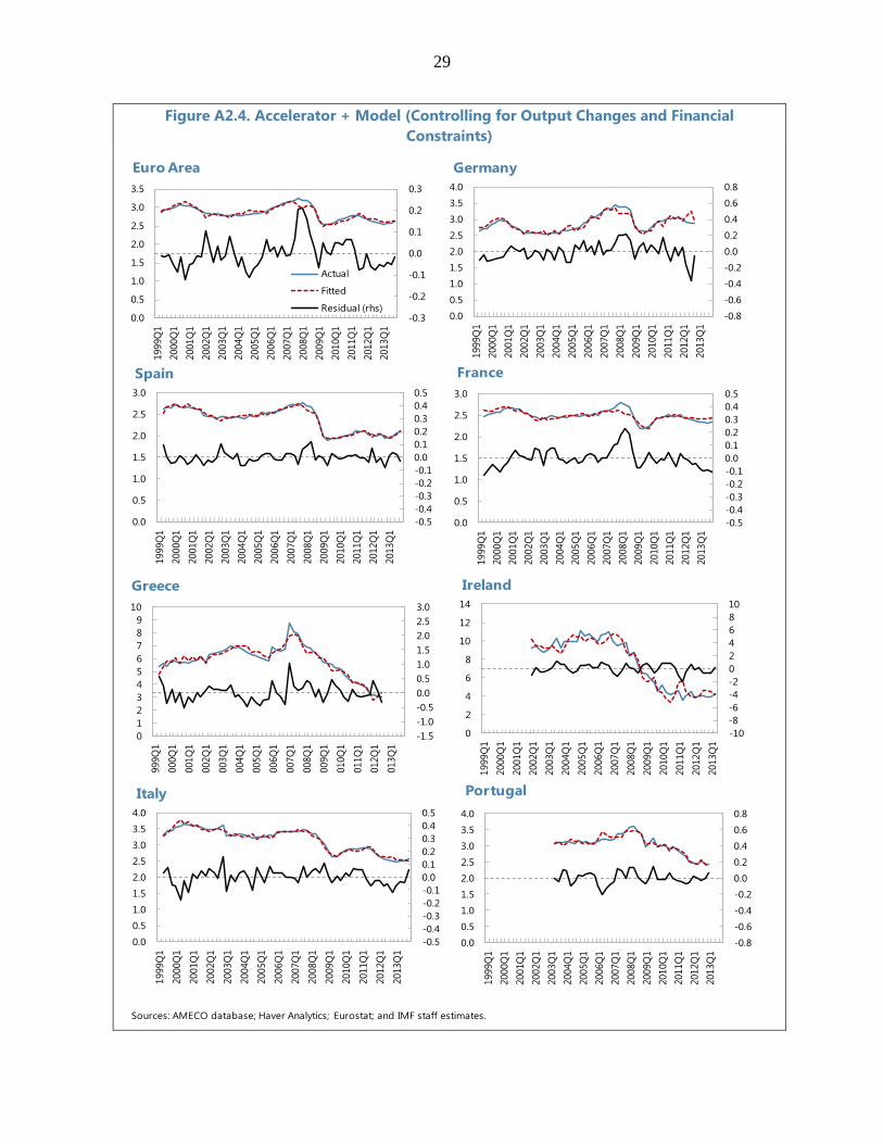
29
Figure A2.4. Accelerator + Model (Controlling for Output Changes and Financial
Constraints)
Figure 4. Bond Market Model
(Controlling For Output Changes And Financial Constraints)
Sources: AMECO database; Haver Analytics; Eurostat; and IMF staff estimates.
-0.5
-0.4
-0.3
-0.2
-0.1
0.0
0.1
0.2
0.3
0.4
0.5
0.0
0.5
1.0
1.5
2.0
2.5
3.0
1999Q
1
2000Q
1
2001Q
1
2002Q
1
2003Q
1
2004Q
1
2005Q
1
2006Q
1
2007Q
1
2008Q
1
2009Q
1
2010Q
1
2011Q
1
2012Q
1
2013Q
1
France
-0.5
-0.4
-0.3
-0.2
-0.1
0.0
0.1
0.2
0.3
0.4
0.5
0.0
0.5
1.0
1.5
2.0
2.5
3.0
1999Q
1
2000Q
1
2001Q
1
2002Q
1
2003Q
1
2004Q
1
2005Q
1
2006Q
1
2007Q
1
2008Q
1
2009Q
1
2010Q
1
2011Q
1
2012Q
1
2013Q
1
Spain
-1.5
-1.0
-0.5
0.0
0.5
1.0
1.5
2.0
2.5
3.0
0
1
2
3
4
5
6
7
8
9
10
1999Q
1
2000Q
1
2001Q
1
2002Q
1
2003Q
1
2004Q
1
2005Q
1
2006Q
1
2007Q
1
2008Q
1
2009Q
1
2010Q
1
2011Q
1
2012Q
1
2013Q
1
Greece
-0.8
-0.6
-0.4
-0.2
0.0
0.2
0.4
0.6
0.8
0.0
0.5
1.0
1.5
2.0
2.5
3.0
3.5
4.0
1999Q
1
2000Q
1
2001Q
1
2002Q
1
2003Q
1
2004Q
1
2005Q
1
2006Q
1
2007Q
1
2008Q
1
2009Q
1
2010Q
1
2011Q
1
2012Q
1
2013Q
1
Germany
-0.5
-0.4
-0.3
-0.2
-0.1
0.0
0.1
0.2
0.3
0.4
0.5
0.0
0.5
1.0
1.5
2.0
2.5
3.0
3.5
4.0
1999Q
1
2000Q
1
2001Q
1
2002Q
1
2003Q
1
2004Q
1
2005Q
1
2006Q
1
2007Q
1
2008Q
1
2009Q
1
2010Q
1
2011Q
1
2012Q
1
2013Q
1
Italy
-0.8
-0.6
-0.4
-0.2
0.0
0.2
0.4
0.6
0.8
0.0
0.5
1.0
1.5
2.0
2.5
3.0
3.5
4.0
1999Q
1
2000Q
1
2001Q
1
2002Q
1
2003Q
1
2004Q
1
2005Q
1
2006Q
1
2007Q
1
2008Q
1
2009Q
1
2010Q
1
2011Q
1
2012Q
1
2013Q
1
Portugal
-10
-8
-6
-4
-2
0
2
4
6
8
10
0
2
4
6
8
10
12
14
1999Q
1
2000Q
1
2001Q
1
2002Q
1
2003Q
1
2004Q
1
2005Q
1
2006Q
1
2007Q
1
2008Q
1
2009Q
1
2010Q
1
2011Q
1
2012Q
1
2013Q
1
Ireland
-0.3
-0.2
-0.1
0.0
0.1
0.2
0.3
0.0
0.5
1.0
1.5
2.0
2.5
3.0
3.5
1999Q
1
2000Q
1
2001Q
1
2002Q
1
2003Q
1
2004Q
1
2005Q
1
2006Q
1
2007Q
1
2008Q
1
2009Q
1
2010Q
1
2011Q
1
2012Q
1
2013Q
1
Euro Area
Actual
Fitted
Residual (rhs)
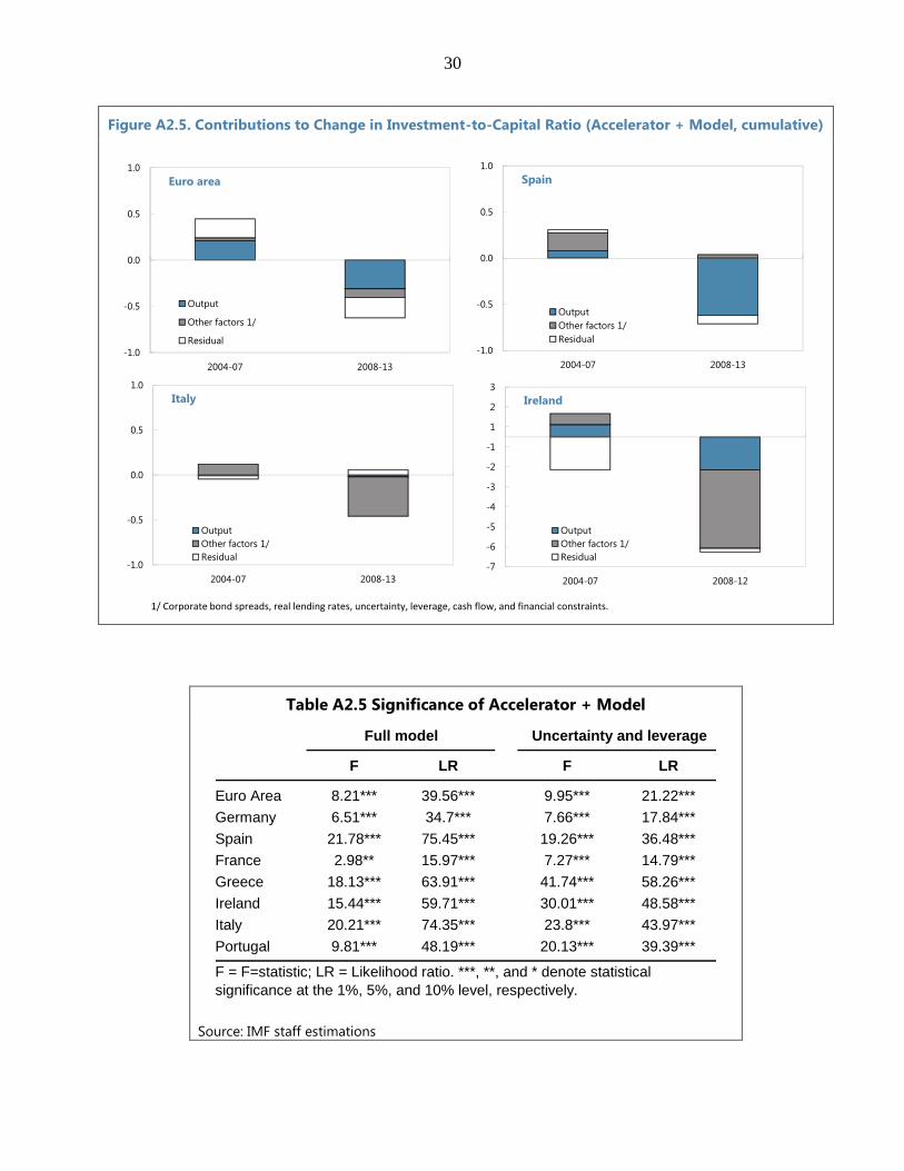
30
Figure A2.5. Contributions to Change in Investment-to-Capital Ratio (Accelerator + Model, cumulative)
Table A2.5 Significance of Accelerator + Model
Source: IMF staff estimations
-1.0
-0.5
0.0
0.5
1.0
2004-07 2008-13
Spain
Output
Other factors 1/
Residual
-7
-6
-5
-4
-3
-2
-1
1
2
3
2004-07 2008-12
Ireland
Output
Other factors 1/
Residual-1.0
-0.5
0.0
0.5
1.0
2004-07 2008-13
Italy
Output
Other factors 1/
Residual
1/ Corporate bond spreads, real lending rates, uncertainty, leverage, cash flow, and financial constraints.
-1.0
-0.5
0.0
0.5
1.0
2004-07 2008-13
Euro area
Output
Other factors 1/
Residual
Table 5.
F LR F LR
Euro Area 8.21*** 39.56*** 9.95*** 21.22***
Germany 6.51*** 34.7*** 7.66*** 17.84***
Spain 21.78*** 75.45*** 19.26*** 36.48***
France 2.98** 15.97*** 7.27*** 14.79***
Greece 18.13*** 63.91*** 41.74*** 58.26***
Ireland 15.44*** 59.71*** 30.01*** 48.58***
Italy 20.21*** 74.35*** 23.8*** 43.97***
Portugal 9.81*** 48.19*** 20.13*** 39.39***
Full model Uncertainty and leverage
F = F=statistic; LR = Likelihood ratio. ***, **, and * denote statistical
significance at the 1%, 5%, and 10% level, respectively.