1

For the sake of simplicity, investors often rely heavily on portfolio characteristics to understand their investment portfolios. For instance, a 2,000 security multi-asset portfolio can be quickly analyzed by simply knowing its market beta, leverage, total risk, yield, and duration – the last two measures are fixed income analytics. Armed with just a few characteristics, many investors feel confident in their ability to make predictive assessments regarding the future behavior of their portfolio. While these portfolio characteristics are elegant in their simplicity, it is important to understand their limitations. In this note we focus on the often ignored limitations of using duration as a risk measure, especially in a multi-asset portfolio. We highlight the implications of ignoring the non-stationarity of yield volatility, the lack of a global yield curve, the uncertainty of inflation linked bond cashflows, and the impact of diversifying assets in a multi-asset portfolio. Given these limitations we encourage our readers to exercise great caution in making predictive assessments based on a portfolio’s reported duration.

Don’t Forget About Yield Volatility

The price of an option-free bond moves in the opposite direction of its yield change. While this directional relationship is universal, there are two characteristics that impact the magnitude of the price change. The first is the coupon of the bond. All else equal, the price of bonds with smaller or zero coupons are more sensitive to changes in yields relative to bonds with larger coupons. The second is the bond’s maturity. All else equal, the prices of bonds with longer maturities are more sensitive to changes in yield than bonds with shorter maturities. The fundamental intuition behind this is the difference in reinvestment risk. The sooner interest and principal cashflows are received, the faster they can be reinvested at the prevailing market yields, making them less sensitive to changes in prevailing market yields. In an effort to quantify a bond’s price sensitivity to changes in yield, Frederick Macaulay1 formulated the now ubiquitous duration measure. Duration is designed to measure the time-weighted cashflows of a bond and is measured in years.

= × ×

Where: k=number of annual coupon payments n=number of years until maturity t=period of cashflow PVCF_t =discounted present value of time t’s cashflow PVTCF =dirty price of the bond

1 Frederick Macaulay, “Some Theoretical Problems Suggested by the Movement of Interest Rates, Bond Yields, and Stock Prices in the U.S. Since 1856”, National Bureau of Economic Research, 1938

March 2017

Investment Insight: Don’t Judge a Portfolio by its Duration

Edward Qian, Ph.D., CFA and Bryan Belton, CFA

2

A minor modification of Macaulay duration offers a first order approximation for the expected price change of a bond given a parallel instantaneous change in yields.

= Macaulayduration1 Yield

As a result, the expected return of a bond given a change in yields can be approximated by: Modifiedduration × Yieldchange × 100

The ability to simply estimate changes in bond prices given changes in yields makes duration a powerful tool. However, it is important to be mindful of duration’s limitations, while also ensuring it is not applied beyond its designed use. For example, it is inappropriate to use duration as a predictor of either absolute or relative return volatility as one would need to assume that yield volatility is uniform, both on a cross-sectional basis (i.e. across the term structure and across countries) as well as on a time series basis (i.e. across time). Based on the equation above, the price volatility of a bond is its modified duration times the volatility of its yield change. Duration is only half of the equation -literally. Ignoring yield volatility invalidates any conclusion about price returns or return volatility that is drawn from duration alone. This can clearly be seen by looking at the relationship between return volatility and duration of the Barclays Global Treasury Index over the past 25 years.

Exhibit 1 charts the yield to maturity, weighted average maturity, and the duration of the Barclays Global Treasury Index from 1990-2017. Since 1990, the index’s yield to maturity has plummeted from 8.8% to its current level of 1%. The mathematics of duration suggests that lower yields should force duration

higher. Exhibit 1 shows that duration has indeed increased. In 1990 the duration of the Barclays Global Treasury Index was 4.9 years. Today the index’s duration is 7.9 years which is 62% higher than it was 25 years ago. While the weighted average maturity of the index has increased from 8 years in 1990 to 9.4 years today, the duration extension has been primarily driven by declining yields rather than longer dated issuance. Assuming yield volatility has been stationary over time, one would expect that the return volatility of the Global Treasury index has increased in response to the increase in its duration. To test this

For illustrative purposes only. Source: PanAgora.

Exhibit 1: Barclays Global Treasury Index 1990-2017

3

assumption, we estimate return volatility using monthly, hedged returns for the Barclays Global Treasury Index starting in 1987. We apply declining weights to past monthly returns with an adaptive exponential decay with a two-year half-life. The results of this estimation are summarized in Exhibit 2 which plots the index’s rolling return volatility with its duration from 1990 to 2017.

Despite a 62% increase in the index’s duration since 1990, the index’s return volatility has actually declined by 28% over the same period. This suggests that duration has been a failed measure of risk. Of course the explanation behind this seemingly paradoxical paradigm is

yield volatility. As the yield of the index has declined over time, so has the volatility of yield changes. Smaller changes in yields have resulted in smaller changes in bond prices despite the fact that a longer duration has made bond prices more sensitive to changes in yields. The declining return volatility yet extending duration of sovereign bond indices has important implications for investors. In 1990, the Barclays Global Treasury Index had return volatility of 4.24% and a duration of 4.9 years. Today, the same index has return volatility of 3.05% and a duration of 7.9 years. To match the return volatility that sovereign bond index investors experienced 25 years ago, investors would need to hypothetically lever today’s index 1.4X and extend its duration to 10.9 years! For investors who manage their asset allocation to a fixed weight capital budget (e.g. 60/40), their portfolio’s duration has been on the rise, but the risk contribution from fixed income has been on the decline. For risk based asset allocators like Risk Parity, portfolio duration would have had to increase by 225% to maintain the fixed income risk contribution at a similar level to what it was in 1990. While we are unaware of any Risk Parity strategies that were live in 1990, we use this example to illustrate that a change in a portfolio’s duration does not necessarily reflect a change in fixed income’s influence on a portfolio. Consequently, it is also not a valid justification to reduce fixed income exposure.

Duration in a Global Context

Duration can approximate a bond portfolio’s expected change in return for an instantaneous, parallel shock of a singular yield curve. Unfortunately, a single yield curve does not exist in a world with independent central banks, divergent monetary policy, fiscal policy, inflation, and growth. Differences in the macroeconomic condition can cause yield curves to look very different across countries in both level and shape. Our brief analysis of the Barclays Global Treasury Index shows that yield volatility has not been

For illustrative purposes only. Source: PanAgora.

Exhibit 2: Barclays Global Treasury Index 1990-2017

4

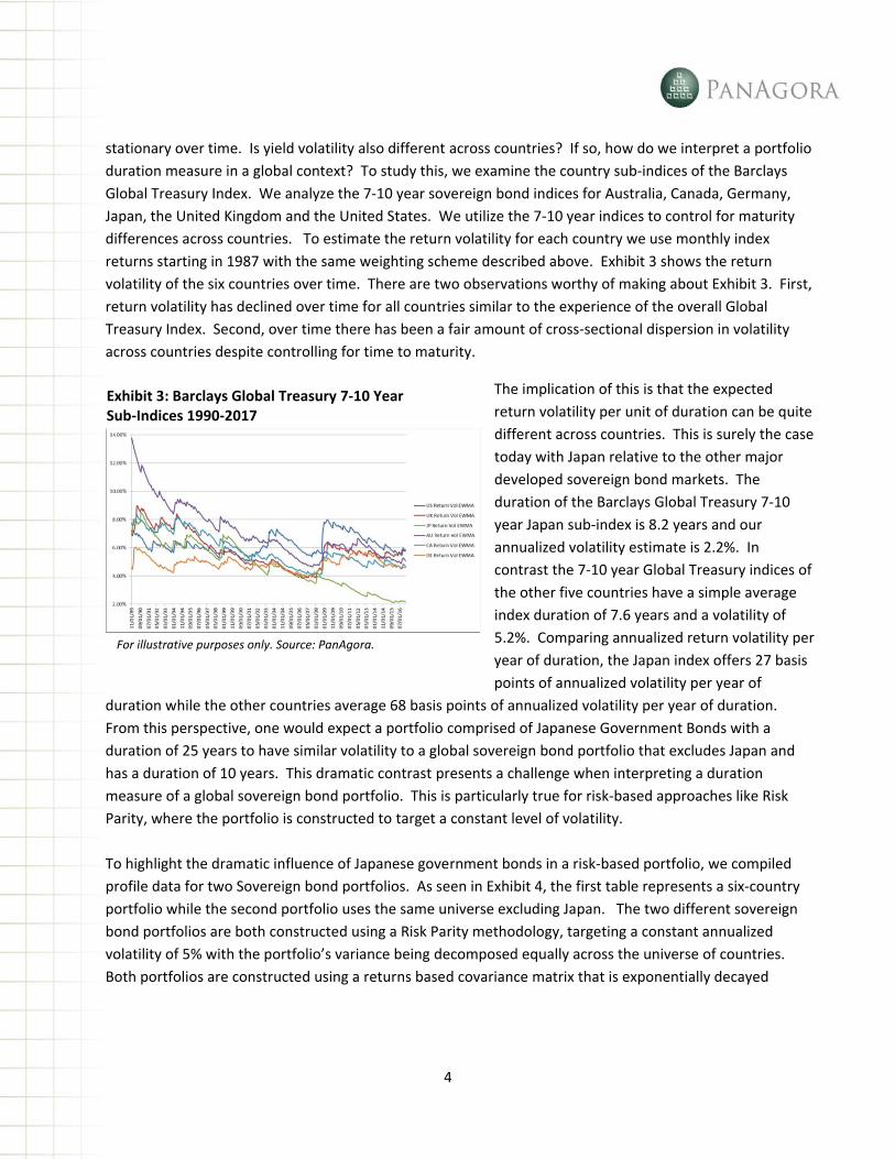
stationary over time. Is yield volatility also different across countries? If so, how do we interpret a portfolio duration measure in a global context? To study this, we examine the country sub-indices of the Barclays Global Treasury Index. We analyze the 7-10 year sovereign bond indices for Australia, Canada, Germany, Japan, the United Kingdom and the United States. We utilize the 7-10 year indices to control for maturity differences across countries. To estimate the return volatility for each country we use monthly index returns starting in 1987 with the same weighting scheme described above. Exhibit 3 shows the return volatility of the six countries over time. There are two observations worthy of making about Exhibit 3. First, return volatility has declined over time for all countries similar to the experience of the overall Global Treasury Index. Second, over time there has been a fair amount of cross-sectional dispersion in volatility across countries despite controlling for time to maturity.

The implication of this is that the expected return volatility per unit of duration can be quite different across countries. This is surely the case today with Japan relative to the other major developed sovereign bond markets. The duration of the Barclays Global Treasury 7-10 year Japan sub-index is 8.2 years and our annualized volatility estimate is 2.2%. In contrast the 7-10 year Global Treasury indices of the other five countries have a simple average index duration of 7.6 years and a volatility of 5.2%. Comparing annualized return volatility per year of duration, the Japan index offers 27 basis points of annualized volatility per year of

duration while the other countries average 68 basis points of annualized volatility per year of duration. From this perspective, one would expect a portfolio comprised of Japanese Government Bonds with a duration of 25 years to have similar volatility to a global sovereign bond portfolio that excludes Japan and has a duration of 10 years. This dramatic contrast presents a challenge when interpreting a duration measure of a global sovereign bond portfolio. This is particularly true for risk-based approaches like Risk Parity, where the portfolio is constructed to target a constant level of volatility. To highlight the dramatic influence of Japanese government bonds in a risk-based portfolio, we compiled profile data for two Sovereign bond portfolios. As seen in Exhibit 4, the first table represents a six-country portfolio while the second portfolio uses the same universe excluding Japan. The two different sovereign bond portfolios are both constructed using a Risk Parity methodology, targeting a constant annualized volatility of 5% with the portfolio’s variance being decomposed equally across the universe of countries. Both portfolios are constructed using a returns based covariance matrix that is exponentially decayed

For illustrative purposes only. Source: PanAgora.

Exhibit 3: Barclays Global Treasury 7-10 Year Sub-Indices 1990-2017

5

with a two-year half-life. We use monthly returns from the Barclays Global Treasury 7-10 country sub-indices beginning in 1987. While both of these portfolios represent a global sovereign bond portfolio targeting 5% annualized risk, the leverage and the duration characteristics are noticeably different. The portfolio including Japan has more leverage and a higher duration compared to the portfolio excluding Japan. The reality is that these portfolios are more similar than they are different, but that would not be the conclusion drawn based on the 3.5 year duration gap between the two portfolios. While deciding whether to include or exclude Japanese Government Bonds in a sovereign bond portfolio is outside the scope of this paper, we

do note that low volatility and low yielding bonds have been attractive sources of risk-adjusted returns. In fact, in a recent Investment Insight2 we show that German and Japanese government bonds were two of the highest returning sovereign bond markets in 2016. While the low volatility craze in equities continues to grow, it appears it has not garnered much support in fixed income investing. It makes one wonder if the duration of low volatility fixed income assets played a role in curbing investors’ enthusiasm.

The Problem with Duration and Inflation Linked Bonds

Duration measures the time-weighted, discounted cashflows over the remaining life of a bond. Assuming no credit risk, duration is an easy measure to accurately calculate for bonds with fixed coupon payments, delivered over a fixed schedule. For bonds with uncertain cashflows over time, the reliability of the duration calculation can break down. This is the case with inflation linked bonds as the sizes of both the coupon payments, as well as the principal payment at maturity, adjust over time based on realized inflation. The uncertainty in future cashflows leaves us with uncertainty regarding an inflation linked bond’s actual duration. While all imperfect, there are three commonly used methods to calculate duration for an inflation linked bond. The first, and most commonly used methodology by index providers, uses uninflated or real cashflows to estimate duration. For an inflation linked bond priced at par, the bond’s stated coupon is assumed to be the fixed cashflow over time and the original par amount is assumed to be the last cashflow received at the bond’s maturity.

Since an inflation linked bond’s real yield will be lower than the nominal yield of an equivalent treasury bond, its duration will also be longer. Exhibit 5 compares the index duration of the Barclays US Treasury 7-

2 Investment Insight, “2016 Year in Review- A Royal Flush for Risk Parity,” Edward Qian, Bryan Belton, January 2017.

Risk Weight Risk Contribution Duration US 5.7% 17.4% 16.6% 7.6 UK 5.9% 18.0% 16.6% 7.5 JP 2.2% 59.4% 16.7% 8.2 AU 5.1% 21.5% 16.7% 7.2 CA 4.7% 22.2% 16.7% 7.6 DE 4.6% 22.6% 16.7% 8.0 Total 5.0% 161.2% 100.0% 12.6

Risk Weight Risk Contribution Duration

US 5.7% 20.9% 20.0% 7.6 UK 5.9% 20.9% 20.0% 7.5 AU 5.1% 25.0% 20.0% 7.2 CA 4.7% 26.2% 20.0% 7.6 DE 4.6% 26.9% 20.0% 8.0 Total 5.0% 119.9% 100.0% 9.1

For illustrative purposes only. Source: PanAgora.

Exhibit 4: Risk Parity Sovereign Bond Portfolios

6

10 year index relative to the Barclays US Inflation Linked 7-10 year index. Despite controlling for maturity, the inflation linked index exhibits persistently higher duration over time. The duration difference between

these two indices is largely explained by the difference between using real and nominal cashflows to calculate duration. This creates an apples-to-oranges comparison and muddies the interpretation of a duration measure for a portfolio holding both nominal and inflation linked bonds. The second approach calculates duration based on inflated cashflows. This approach requires a forecast or, at a minimum, an assumption about future inflation in order to inflate cashflows over the life of the bond. Bloomberg uses this approach as

their default Macaulay duration measure which can be retrieved with the mnemonic “Dur_Mid.” To adjust cashflows over time the default assumption is that future inflation will change at a rate equal to the previous 12 month change in the Reference Consumer Price Index. While using inflated cashflows allows for a more meaningful comparison between nominal and inflation linked bonds, estimated duration is very sensitive to the inflation forecast that is used. The third methodology used to estimate duration is an empirical approach. The empirical measure considers the historical relationship between movements of nominal yields and real yields via regression. The regression derives a beta of real yield movements with respect to the nominal curve. This beta can then be applied as a scalar to the duration measure based on unadjusted cashflows to create an empirical duration measure for inflation linked bonds.

Exhibit 6 compares the two different duration measures estimated by Barclays for their US Inflation Linked 7-10 year sub-index from 2004 to 2017. The OAD measure represents the modified duration based on the real or unadjusted cashflows of the index. The empirical duration scales OAD by a yield beta that represents the sensitivity between real and nominal yields. While this approach is intuitively appealing, it requires

For illustrative purposes only. Source: PanAgora.

Exhibit 5: Duration Comparison Inflation Linked vs. Nominal

For illustrative purposes only. Source: PanAgora.

Exhibit 6: Barclays US Inflation Linked 7-10 Year Index

For illustrative purposes only. Source: PanAgora.

7

some subjectivity in estimating the yield beta and it can produce wild swings in estimated duration. For example the empirical duration of the index was 6.3 years at the end

of April 2013, but four months later it jumped over 40% to 9.1 years. In contrast, the unadjusted duration only increased 1-month. Exhibit 7 compares the three different measures for the current on-the-run US 10-year inflation linked bond. Real OAD represents Bloomberg’s estimate of modified duration based on unadjusted or real cashflows. Nominal OAD represents Bloomberg’s estimate of modified duration based on inflation adjusted cashflows. The inflation adjustment applies the trailing 12-month change in CPI forward as an annual adjustment for the remaining life of the bond. Empirical OAD represents Barclays POINT’s estimate of duration. This approach scales the unadjusted duration measure by a regressed yield beta which measures the sensitivity of real yields to nominal yields. The Real OAD measure is twice as long as the Nominal OAD measure, while the Empirical OAD measure is right in the middle of the other two. The fact that the same on-the-run bond can have three very different duration measures highlights the limitations of duration in a portfolio with both nominal and inflation linked bonds.

The Duration Impact of Diversifying Assets

Up until this point, we have focused our discussion on the limitation of duration as a risk measure in fixed income portfolios. It turns out that duration becomes an even more limited measure in the context of diversified multi-asset portfolios. This is particularly true in a Risk Parity portfolio where the risk contribution across fixed income, equities, and inflation protected assets are typically balanced. When calculating the duration of a portfolio, the fixed income positions contribute to portfolio duration while the equity and commodity positions are assumed to have zero duration. It can be argued that this is an inappropriate way to calculate portfolio duration because it fails to take into consideration any interest rate sensitivity of equities and commodities investments. For instance, if interest rates rise sharply due to stronger than expected growth or higher than expected inflation, the portfolio’s equity or commodity positions should create a return offset respectively to buffer some of the loss contribution expected from the fixed income positions. If so, the portfolio’s sensitivity to yield changes should be lower than what would be otherwise implied by portfolio duration from fixed income investments alone. It turns out we see this in practice.

Exhibit 8 shows the duration3 of PanAgora’s Risk Parity Multi Asset portfolio as of February 2017 as well as the expected portfolio return if we experienced a 100 basis point parallel shock in the

3 Duration of the portfolio includes a position in Japanese Government bonds. In addition, we use a real measure duration for inflation linked bonds is calculated with unadjusted cashflows.

Real OAD Nominal OAD Empirical OAD

10 YR OTR TIP 9.6 4.8 7.3

Hypothetical Impact PAM RPMA Feb 2017

Duration 13.7 years

100 bps shock in US Yield Curve -7.5%

Exhibit 7: Duration Measures for TII 0 3/8 01/15/27

Exhibit 8: PanAgora Risk Parity Portfolio Feb 2017

Projected returns are hypothetical and for illustrative purposes only. Past performance is not a guarantee of future results. See additional disclosure.

For illustrative purposes only. Source: PanAgora.

8

US yield curve. Both measures are calculated using the Barclays POINT risk model. If the US yield curve jumped higher by 100 basis points, the return approximation for this portfolio would be -13.7%, based on duration alone. Instead, the POINT multi-asset factor based risk model estimates a drawdown of only -7.5% in this scenario. This implies that the risk model expects either equities, inflation protected assets or possibly both to provide diversifying offsets to the long duration assets in the portfolio. Exhibit 9 measures the rolling 3-year beta to the US Treasury 7-10 year index of both our live Risk Parity composite performance as well as our current portfolio simulated back in time. We measure the beta as the ratio of the covariance between Risk Parity and US Treasury Index 36 month rolling returns, relative to the variance of the 36 month rolling returns of the US Treasury Index. Over the whole sample starting in 1999, the Risk Parity portfolio’s beta to the US Treasury index has been 1.33. A beta greater than 1 reflects the difference in volatility between the Risk Parity portfolio’s annualized volatility target of 10% and the US

Treasury 7-10 year index’s annualized realized volatility of 2.9%. What’s most interesting about the rolling beta is that it exhibits great variability. While the risk contribution target of fixed income in today’s portfolio is held constant back in time, the portfolio’s ex-post beta to US Treasuries has been anything but constant. In fact, its 3-year rolling beta to US Treasuries turns slightly negative at the end of 2012. Exhibit 10 analyzes the sub-period from 2010 to 2012 where Risk Parity’s beta to the US Treasury index turned negative. This three-year stretch proved to be a strong period for Risk Parity, as the three major asset classes all beat cash and they proved to be diversifying to one another. Despite the portfolio maintaining a long duration position throughout this period, its empirical beta to the US Treasury index was effectively zero as the portfolio’s diversifying exposure to commodities and global equities were very negatively correlated with US Treasuries during this period. In this case, the impact of strongly diversifying assets eliminated the portfolio’s sensitivity to changes in interest rates. This result proved to be at odds with any conclusion that could have been drawn by the portfolio’s duration measure.

2010-2012 Return Correlation with UST

Current Portfolio 15.15% -0.03

RP Composite 14.89% -0.02

UST 7-10Y IDX 4.53% 1.00

GSCI 2.54% -0.50

MSCI 6.93% -0.55

-50%

0%

50%

100%

150%

200%

250%

300%

12

/1/2

00

24

/1/2

00

38

/1/2

00

31

2/1

/20

03

4/1

/20

04

8/1

/20

04

12

/1/2

00

44

/1/2

00

58

/1/2

00

51

2/1

/20

05

4/1

/20

06

8/1

/20

06

12

/1/2

00

64

/1/2

00

78

/1/2

00

71

2/1

/20

07

4/1

/20

08

8/1

/20

08

12

/1/2

00

84

/1/2

00

98

/1/2

00

91

2/1

/20

09

4/1

/20

10

8/1

/20

10

12

/1/2

01

04

/1/2

01

18

/1/2

01

11

2/1

/20

11

4/1

/20

12

8/1

/20

12

12

/1/2

01

24

/1/2

01

38

/1/2

01

31

2/1

/20

13

4/1

/20

14

8/1

/20

14

12

/1/2

01

44

/1/2

01

58

/1/2

01

51

2/1

/20

15

4/1

/20

16

8/1

/20

16

12

/1/2

01

6

Current Port Beta

Composite Beta

Exhibit 9: Simulated Rolling Beta to US 7-10 Treasury

Simulated returns are hypothetical and for illustrative purposes only. Past performance is not a guarantee of future results. See additional disclosure.

Exhibit 10: Risk Parity Simulation 2010-2012

Simulated returns are hypothetical and for illustrative purposes only. Past performance is not a guarantee of future results. See additional disclosure.

9

Summary

In this note we raise several concerns regarding the appropriateness of using duration as a risk measure for a multi-asset portfolio. First, we point out that duration is only half of the equation and that yield volatility deserves equal consideration. Yield volatility has not been stationary either across time or countries. The implication of time varying yield volatility is that duration measures are not comparable across time or countries. A global treasury portfolio with a duration of 5 years in 1990 is equivalent to a global treasury portfolio with a duration of 11 years or a Japanese Government Bond portfolio with a duration of 16 years today. Inflation linked bonds introduce another complication to measuring duration as their cashflows are variable with inflation over time. The calculation methodology used to estimate the duration of inflation linked bonds can result in dramatically different measurements. Finally, the stated measure of portfolio duration in a diversified multi-asset portfolio tends to overestimate the portfolio’s actual sensitivity to yield changes, as uncorrelated and conditionally negatively correlated assets can provide meaningful return offsets to the long duration assets in a portfolio. Given these collective limitations, we caution our readers against judging any portfolio, whether it is a nominal or inflation-linked fixed income portfolio, or a multi-asset portfolio, by its duration.

10

Legal Disclosures

This material is solely for informational purposes and shall not constitute an offer to sell or the solicitation to buy securities. The opinions expressed herein represent the current, good faith views of the author(s) at the time of publication and are provided for limited purposes, are not definitive investment advice, and should not be relied on as such. The information presented in this article has been developed internally and/or obtained from sources believed to be reliable; however, PanAgora Asset Management, Inc. ("PanAgora") does not guarantee the accuracy, adequacy or completeness of such information. Predictions, opinions, and other information contained in this article are subject to change continually and without notice of any kind and may no longer be true after the date indicated. Any forward-looking statements speak only as of the date they are made, and PanAgora assumes no duty to and does not undertake to update forward-looking statements. Forward-looking statements are subject to numerous assumptions, risks and uncertainties, which change over time. Actual results could differ materially from those anticipated in forward-looking statements. This material is directed exclusively at investment professionals. Any investments to which this material relates are available only to or will be engaged in only with investment professionals. There is no guarantee that any investment strategy will achieve its investment objective or avoid incurring substantial losses.

Limitations of Hypothetical Performance. The discussion in this material poses a number of projected, simulated, and otherwise hypothetical scenarios that rely on a number of assumptions. Certain of the assumptions have been made for modeling purposes and are unlikely to be realized. No representation or warranty is made as to the reasonableness of the assumptions made or that all assumptions made in the discussion herein have been stated or fully considered. The discussion of hypothetical scenarios have many inherent limitations and may not reflect the impact that material economic and market factors may have had on the decision-making process if client funds are actually managed in the manner shown. Actual operating results, asset values, timing and manner of dispositions or other realization events and resolution of other factors taken into consideration may differ materially from the assumptions upon which hypothetical information is based. Changes in the assumptions may have a material impact on the hypothetical returns presented. Hypothetical returns do not reflect the actual returns of any portfolio strategy and do not guarantee future results. Actual results experienced by clients may vary significantly from the hypothetical illustrations shown.

Projected returns are hypothetical in nature and are shown for illustrative, informational purposes only. This material is not intended to forecast or predict future events, but rather to demonstrate the investment process of PanAgora. Specifically, the projected returns are based upon a variety of estimates and assumptions described in this material. Projected Returns May Not Materialize.

Simulated returns are hypothetical in nature and are shown for illustrative, informational purposes only. This material is not intended to exhibit how any PanAgora strategy would have performed over time, but rather to demonstrate the investment process of PanAgora. Since simulated returns do not represent actual trading, results may have under- or over-compensated for the impact, if any, of certain market factors, such as lack of liquidity, and may not reflect the impact that certain economic or market factors may have had on

11

the decision-making process. Simulated performance also is developed with the benefit of hindsight. Other periods selected may have different results.

PanAgora is exempt from the requirement to hold an Australian financial services license under the Corporations Act 2001 in respect of the financial services. PanAgora is regulated by the SEC under U.S. laws, which differ from Australian laws.

Past performance is not a guarantee of future results. Performance shown is supplemental to the GIPS composite disclosures provided herewith. Please review the composite performance prior to drawing any inferences regarding PanAgora’s past performance from this material.

For institutional use only.

318031 / AA35 2/1/2017

PERFORMANCE DISCLOSURE

Risk Parity Multi-Asset Master Composite Composite: Risk Parity Multi-Asset Master (As of 12/31/2016) Benchmark: 60% MSCI World / 40% Citigroup World Government Bond Index

Year

Composite

Gross of Fees

Return (%)

Composite

Net of Fees

Return (%)

Index

Return (%) High (%)* Low (%)*

3 Yr. Composite

Return (%)***

3 Yr. Composite

Standard

Deviation***

3 Yr. Index

Return (%)***

3 Yr. Index

Standard

Deviation***

2016 13.74 13.39 5.33 13.84 12.44 8.05 8.81 2.10 7.14

2015 -3.45 -3.80 -1.72 -2.64 -4.12 4.73 8.89 4.68 7.07

2014 14.86 14.51 2.80 16.31 13.78 10.91 7.83 8.74 6.92

2013 3.58 3.23 13.54 4.09 3.30 9.75 8.19 7.51 8.74

2012 14.68 14.33 10.15 14.11 13.99 14.89 7.09 6.22 10.96

2011 11.30 10.92 -0.63 11.72 10.17 12.32 8.68 8.91 13.85

2010 18.80 18.40 9.50 19.15 17.79 3.31 12.62 0.05 15.87

2009 7.16 6.79 18.72 7.27 7.23 2.03 12.33 0.19 14.22

2008 -13.39 -13.69 -22.97 -13.13 -14.38 -0.71 11.33 -1.04 10.80

2007 14.43 14.03 9.98 N.A. N.A. N.A. N.A. N.A. N.A.

Year

Composite Assets

($Millions)

Percentage of

Firm Assets (%)

Number of

Accounts

Firm Assets

($Millions)

Non-fee paying

and/or Proprietary

Assets (%)

2016 $5,788.71 13.53 5 $42,798 0.00

2015 $4,015.91 10.47 5 $38,361 0.00

2014 $3,013.93 7.94 4 $37,953 0.00

2013 $1,520.33 3.85 3 $39,533 0.00

2012 $777.78 2.55 4 $30,524 0.00

2011 $249.36 1.11 2 $22,401 0.00

2010 $195.59 0.98 2 $19,914 0.00

2009 $134.30 0.83 2 $16,084 0.00

2008 $55.32 0.43 3 $12,778 4.46

2007 $56.02 0.24 2 $25,480 10.55

*High/Low Returns have not been provided for composites with less than two accounts in the composite for the entire year.

***Three year returns and standard deviations have not been provided for composites with fewer than 36 months of monthly returns

One Year Performance Internal Dispersion External Dispersion

Assets Under Management

Firm Overview PanAgora Asset Management, Inc. (the “Firm”) claims compliance with the Global Investment Performance Standards (“GIPS®”) and has prepared and presented this report in compliance with the GIPS Standards. PanAgora Asset Management, Inc. has been independently verified for the periods 1993-2015. The verification reports are available upon request. Verification assesses whether (1) the firm has complied with all the composite construction requirements of the GIPS standards on a firm-wide basis and (2) the firm’s policies and procedures are designed to calculate and present performance in compliance with the GIPS standards. Verification does not ensure the accuracy of any specific composite presentation. For the purposes of compliance with GIPS, the Firm is defined as a broad based investment management organization that provides investment services to institutions through separately managed accounts, pooled funds and mutual funds. The Firm is an independent investment advisor registered under the Investment Advisers Act of 1940 specializing in quantitative investment strategies and includes all assets under management. Composition of Composite The accounts within the Risk Parity Multi-Asset Master Composite seek to generate attractive, absolute risk-adjusted returns utilizing a multi-asset investing approach through a combination of strategic asset allocation and tactical portfolio management. The strategy seeks to deliver true diversification through balanced risk budgeting between equities, bonds and commodities. The Composite consists of portfolios deploying a Risk Parity Multi-Asset approach to asset allocation that target an expected annualized volatility of 10%. The Composite is comprised of all discretionary institutional accounts managed by the Firm in this investment style. The inception date for the Composite is January 1, 2006. The creation date for the Composite was February 15, 2012. There is a minimum of $2 million in assets for inclusion in this composite. The Risk Parity Multi-Asset strategy employs leverage in its risk efficient asset allocation portfolios in order to achieve the expected risk levels, predominantly through the use of exchange traded futures, forward contracts and swaps. In normal market conditions, the gross notional exposure of long and short positions has typically represented up to four times the market value of a client's account. The extent of leverage will vary by client.

318031 / AA35 2/1/2017

PERFORMANCE DISCLOSURE

New portfolios are included in a GIPS composite beginning with the first complete month of performance in the strategy. Terminated portfolios are included through the final full month of management. Composites may include portfolios with certain existing investment restrictions that the Company believes do not materially impact the investment strategy. A list of composite descriptions is available upon request. Calculation of Composite A composite's monthly return is computed by asset weighting the portfolio returns within the composite, using the beginning of period market values. The quarterly return of a composite is computed by geometrically linking the returns of each month within the calendar quarter. The annual return of a composite is computed by geometrically linking the returns of each quarter within the calendar year. Investments held by all portfolios are valued on a trade-date basis using accrual accounting. Individual portfolio returns are calculated using the daily time-weighted rate of return (TWRR) methodology. Performance is expressed in U.S. dollars. Policies for valuing portfolios, calculating performance, and preparing compliant presentations are available upon request. Returns are net of foreign withholding taxes on dividends, interest, and capital gains. Equity benchmark returns assume dividends are reinvested monthly. MSCI benchmarks are

presented net after withholding taxes by applying the maximum rate applicable to non-resident institutional investors who do not benefit from double taxation treaties. Returns

from other benchmark providers are presented gross of any tax withholding.

Index Disclosure The benchmark for this Composite is a fixed blend benchmark, comprised of 60% of the MSCI World Index and 40% of the Citigroup World Government Bond Index each month. The MSCI World Index is a free float-adjusted market capitalization weighted index that captures large and mid-cap representation across 23 Developed Markets (DM) countries. The index covers approximately 85% of the free float-adjusted market capitalization in each country. The Citigroup World Government Bond Index measures the performance of fixed-rate, local currency, investment-grade sovereign bonds. The WGBI is a widely used benchmark that currently comprises sovereign debt from over 20 countries, denominated in a variety of currencies, and has more than 30 years of history available. The WGBI is a broad benchmark providing exposure to the global sovereign fixed income market. Benchmarks are generally taken from published sources and may have different calculation methodologies, pricing times, and foreign exchange sources from the Composite. The effect of those differences is deemed to be immaterial. The securities holdings of the composite may differ materially from those of the index used for comparative purposes. Indexes are unmanaged and do not incur expenses. You cannot invest directly in an index. Gross and Net of Fees Disclosure Gross of Fee returns are net of transaction costs but do not include the deduction of management fees and other expenses that may be incurred in managing an investment account. A portfolio’s return will be reduced by management and other fees. The impact of management fees can be material. Investment returns are reduced by advisory fees as in the following example: Over a five year period, if a $100 portfolio had an annual return of 10% it would grow to $161.05. The net compounded effect of a 35 basis point annual investment management fee (without custody charges) would total $2.55 and result in a portfolio value of $158.51. Net of Fee Return results are calculated as the Gross of Fee Returns minus a model fee equal to the highest standard Management Fee and includes a performance fee incentive, if applicable, that a client invested in this strategy would have paid during the performance period. Fee Schedule The below is the standard fee schedule based on the market value of assets under management and stated on an annual basis. Fees are for investment management services only. Custodial fees are not included in the Net of Fee Returns. 0.35 of 1% of assets under management. This fee schedule has been prepared for informational purposes for the purpose of the Firm’s global compliance with GIPS and should not be construed as an offer or solicitation. Actual fees may vary by client. Past Performance is not a guarantee of future performance. No assurance can be given as to future performance.