ip - perso.lcpc.fr
TRANSCRIPT

1
1 23

2
The Guided Bilateral Filter: When the Joint/Cross
Bilateral Filter Becomes RobustLaurent Caraffa, Jean-Philippe Tarel∗, Member, IEEE, Pierre Charbonnier
Abstract—The bilateral filter and its variants such as theJoint/Cross bilateral filter are well known edge-preserving imagesmoothing tools used in many applications. The reason of thissuccess is its simple definition and the possibility of manyadaptations. The bilateral filter is known to be related to robustestimation. This link is lost by the ad hoc introduction of theguide image in the Joint/Cross bilateral filter. We here propose anew way to derive the Joint/Cross bilateral filter as a particularcase of a more generic filter which we name the Guided bilateralfilter. This new filter is iterative, generic, inherits the robustnessproperties of the Robust bilateral filter and uses a guide image.The link with robust estimation allows us to relate the filterparameters with the statistics of input images. A scheme based onGraduated Non Convexity is proposed, which allows convergingto an interesting local minimum even when the cost functionis non-convex. With this scheme, the Guided bilateral filtercan handle non-Gaussian noise on the image to be filtered. Acomplementary scheme is proposed to handle also non-Gaussiannoise on the guide image even if both are strongly correlated.This allows the Guided bilateral filter to handle situations withmore noise than the Joint/Cross bilateral filter can work withand leads to high Peak Signal to Noise Ratio PSNR values asshown experimentally.
Index Terms—image filtering, image smoothing, Bilateral filter,Joint bilateral filter, Cross bilateral filter, Dual bilateral filter.
I. INTRODUCTION
The bilateral filter [1] is a well known edge-preserving
image smoothing tool. The key idea of the bilateral filter
consists in introducing a photometric weight into the stan-
dard Gaussian filter. The effect of this weight is to cancel
spatial interactions between pixels with an important intensity
difference. Thanks to its properties, the bilateral filter is now
used in many different applications, for instance: sharpness
enhancement [2], upsampling [3], depth map refinement [4],
image editing [5] and fog removal [6].
A good summary on bilateral filter, interpretations, improve-
ments and extensions is given in [7]. In our opinion, there
are five important points to recall. First, the bilateral filter is
connected to the robust estimation of the intensity average in
a neighborhood [8]. Second, the staircase effect which may
be observed in the results can be canceled by using linear
fitting rather constant fitting [9]. Third, the bilateral filter can
Copyright (c) 2015 IEEE. Personal use of this material is permitted.However, permission to use this material for any other purposes must beobtained from the IEEE by sending a request to [email protected].
L. Caraffa and J.-P. Tarel are with the Paris-Est University, IFSTTAR(COSYS/LEPSIS), 14-20 Boulevard Newton, F-77420 Champs-sur-Marne,France, e-mail: [email protected] and [email protected]
P. Charbonnier is with the Cerema (ERA 27 IFSTTAR), 11Rue Jean Mentelin, BP 9, F-67200 Strasbourg, France, e-mail:[email protected]
be extended as the adaptive bilateral filter where the scale
parameter in the photometric weight is selected using the
intensities of the neighbor pixels [2]. Fourth, there are several
ways to improve the computation time of the bilateral filter, for
instance using a grid [10] or using distributive histograms [11].
Fifth, in some situations, information about the structure of the
target image is available under the form of a similar image,
called the guide image. The latter may be used to define a
guide weight which may be introduced, either in place of
the photometric weight (leading to the Joint/Cross bilateral
filter [12], [13]) or in conjunction with it (Dual bilateral
filter [14]). Note that the guide image has also been used alone
in [6], but in a framework different from bilateral filtering.
While the improvements proposed in the second to fourth
points only slightly impact the interpretation of the bilateral
filter in terms of robust estimation, the ad hoc introduction
of the guide in the joint/cross bilateral filter calls for a new
statistical interpretation.
In this paper, we first recall in Section II the link between
the bilateral filter and robust estimation, but we also show,
experimentally, that neither the bilateral filter nor its iterative
version are really robust. In contrast, applying a full Iterative
Reweighted Least Squares (IRLS) iteration leads to the so-
called Robust bilateral filter [15]. In the same spirit, we
propose in Section III to connect the Joint/Cross bilateral and
Dual bilateral filters to robust estimation. This leads us to
extend these filters into a novel one, iterative and robust, the
Guided bilateral filter. All the filters we use or introduce here
are listed in Table I with their main features recalled.
TABLE ICHARACTERISTICS OF THE FILTERS USED OR INTRODUCED IN THE PAPER.
Filter name Spatial Photo. Guide Ref.weight weight weight Iterative Robust or eq.
Gaussian Yes No No one step NoBilateral Yes Yes No one step No [1], (1)
Iterated bilateral Yes Yes No several steps No (1)Robust bilateral Yes Yes No IRLS steps Yes [15], (3)
Joint/Cross bilateral Yes No Yes one step No [13], [12]Dual bilateral No Yes Yes one step No [14]
Guided No No Yes one step No [6]Guided bilateral Yes Yes Yes IRLS steps Yes (8)
In Section IV, a convergence scheme based on Graduated
Non Convexity is proposed for the Guided bilateral filter.
Then, in Section V, we show how the input images statistics
can be used to set the filter parameters and we experiment
with the proposed filter under different kinds of added noise.
These results compare advantageously with results obtained

3
with bilateral, Joint/Cross bilateral, Dual bilateral, and Guided
filters. Finally, in Section VI, the interest of the proposed
filter is illustrated on three applications: flash/no-flash filtering,
depth map refinement and fog removal.
II. BILATERAL FILTER
The bilateral filter proposed in [1] is an extension of the
linear smoothing of images where a photometric weight wp
is introduced as a factor of the spatial weight ws. From the
original image E, the result of the bilateral filter is the image
F given by:
F (x) =
∑
t∈Smws(‖t‖)wp(E(x)− E(x+ t))E(x+ t)
∑
t∈Smws(‖t‖)wp(E(x)− E(x+ t))
(1)
where Sm is, typically, a square window [−m,m]× [−m,m].ws is a symmetrical, decreasing function of the distance ‖t‖from the center of Sm. Usually, wp is also an even and
decreasing function of the intensity.
A. Robust bilateral filter
According to [8], the image F resulting from the bilateral
filter can be interpreted as the first step of the minimization,
with respect to F (x), of the local cost:∑
t∈Sm
ws(‖t‖)φ((F (x)− E(x+ t))2) (2)
When ws(‖t‖) = 1, the minimizer F (x) of the cost is the
robust average of the values E(x+ t), t ∈ Sm. In such a case,
φ characterizes the average noise model on the intensities in
the neighborhood Sm. By canceling the derivative of the sum
in (2) with respect to F (x), we have:∑
t∈Sm
ws(‖t‖)φ′((F (x)− E(x+ t))2)(F (x)− E(x+ t)) = 0
After rearranging the terms and fixing non-linear terms to their
previously computed value, the well-known IRLS algorithm is
obtained, which iteratively minimizes (2):
Fk+1(x) =
∑
t∈Sm
ws(‖t‖)φ′((Fk(x)− E(x+ t))2)E(x+ t)
∑
t∈Sm
ws(‖t‖)φ′((Fk(x)− E(x+ t))2)
(3)
Derivation and proofs of convergence of the IRLS iterations
may be found for instance in [16], [17]. By comparing (1)
with (3), we see that the bilateral filter is the first step of
the IRLS algorithm when wp(u) = φ′(u2) and when it
is initialized with the original image (i.e. F0(x) = E(x)).We name Robust bilateral filter, the IRLS iterations until
convergence.
B. Robustness assessment
On Fig. 1, an original image, chosen for its difficulty
(presence of thin image structures) is shown, along with the
image to be processed, where a Gaussian noise (std s = 5) and
a Salt and Pepper (10%) noise were added. The result with the
Fig. 1. Comparison between bilateral filter, iterated bilateral filter and Robustbilateral filter. First row: left, the original image and right, the noisy image(PSNR = 14.5dB). Second row: result with the bilateral filter after 1 and100 iterations (αp = −1, sp = 70, PSNR = 15.5dB and αp = −1, sp =5, PSNR = 14.6dB, respectively). Third row: result of the Robust bilateralfilter with 10 and 100 iterations (αp = 0.5, sp = 5, PSNR = 28.9dB and28.8dB, respectively).
bilateral filter and after 100 iterations of the bilateral filter is
shown on the second row. Despite the fact that it is related to
robust estimation as previously explained, the bilateral filter
is not robust to non-Gaussian noise in the original image.
The iterative application of the bilateral filter is not robust
to outliers either.
On the contrary, the Robust bilateral filter introduced in the
previous section is robust as illustrated by the results with
10 and 100 iterations, shown on the third row of Fig. 1. It
is important to distinguish between the iterated bilateral filter
and the Robust bilateral filter. Indeed, in the Robust bilateral
filter (3), Fk is compared to the fixed values of E, while, in
the iterative application of the bilateral filter, Fk is compared
to the value obtained from the previous filter application.
Due to its derivation, the Robust bilateral filter is robust to
outliers in the original image, provided that the noise model
is suited to the input and that the correct convergence scheme
is used.
4
−10 −8 −6 −4 −2 0 2 4 6 8 100
0.1
0.2
0.3
0.4
0.5
0.6
0.7
0.8
0.9
1
b
exp(−
φα(b
2))
α=1
α=0.5
α=−0.1
α=−0.5
α=−1
−10 −8 −6 −4 −2 0 2 4 6 8 100
1
2
3
4
5
6
7
8
9
10
b
φα(b
2)
α=1
α=0.5
α=−0.1
α=−0.5
α=−1
−10 −8 −6 −4 −2 0 2 4 6 8 100
0.1
0.2
0.3
0.4
0.5
0.6
0.7
0.8
0.9
1
b
2 φ
’ α(b
2)
α=1
α=0.5
α=−0.1
α=−0.5
α=−1
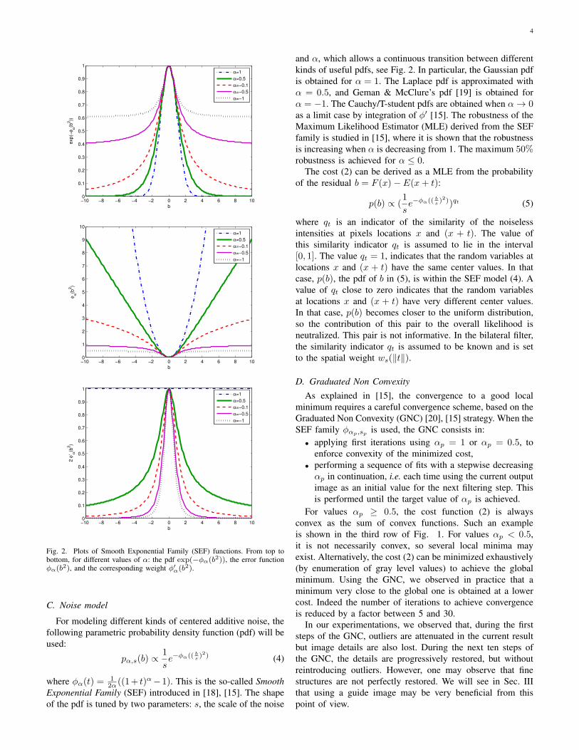
Fig. 2. Plots of Smooth Exponential Family (SEF) functions. From top tobottom, for different values of α: the pdf exp(−φα(b2)), the error functionφα(b2), and the corresponding weight φ′
α(b2).
C. Noise model
For modeling different kinds of centered additive noise, the
following parametric probability density function (pdf) will be
used:
pα,s(b) ∝1
se−φα(( b
s)2) (4)
where φα(t) =12α ((1+ t)α−1). This is the so-called Smooth
Exponential Family (SEF) introduced in [18], [15]. The shape
of the pdf is tuned by two parameters: s, the scale of the noise
and α, which allows a continuous transition between different
kinds of useful pdfs, see Fig. 2. In particular, the Gaussian pdf
is obtained for α = 1. The Laplace pdf is approximated with
α = 0.5, and Geman & McClure’s pdf [19] is obtained for
α = −1. The Cauchy/T-student pdfs are obtained when α → 0as a limit case by integration of φ′ [15]. The robustness of the
Maximum Likelihood Estimator (MLE) derived from the SEF
family is studied in [15], where it is shown that the robustness
is increasing when α is decreasing from 1. The maximum 50%robustness is achieved for α ≤ 0.
The cost (2) can be derived as a MLE from the probability
of the residual b = F (x)− E(x+ t):
p(b) ∝ (1
se−φα(( b
s)2))qt (5)
where qt is an indicator of the similarity of the noiseless
intensities at pixels locations x and (x + t). The value of
this similarity indicator qt is assumed to lie in the interval
[0, 1]. The value qt = 1, indicates that the random variables at
locations x and (x + t) have the same center values. In that
case, p(b), the pdf of b in (5), is within the SEF model (4). A
value of qt close to zero indicates that the random variables
at locations x and (x + t) have very different center values.
In that case, p(b) becomes closer to the uniform distribution,
so the contribution of this pair to the overall likelihood is
neutralized. This pair is not informative. In the bilateral filter,
the similarity indicator qt is assumed to be known and is set
to the spatial weight ws(‖t‖).
D. Graduated Non Convexity
As explained in [15], the convergence to a good local
minimum requires a careful convergence scheme, based on the
Graduated Non Convexity (GNC) [20], [15] strategy. When the
SEF family φαp,sp is used, the GNC consists in:
• applying first iterations using αp = 1 or αp = 0.5, to
enforce convexity of the minimized cost,
• performing a sequence of fits with a stepwise decreasing
αp in continuation, i.e. each time using the current output
image as an initial value for the next filtering step. This
is performed until the target value of αp is achieved.
For values αp ≥ 0.5, the cost function (2) is always
convex as the sum of convex functions. Such an example
is shown in the third row of Fig. 1. For values αp < 0.5,
it is not necessarily convex, so several local minima may
exist. Alternatively, the cost (2) can be minimized exhaustively
(by enumeration of gray level values) to achieve the global
minimum. Using the GNC, we observed in practice that a
minimum very close to the global one is obtained at a lower
cost. Indeed the number of iterations to achieve convergence
is reduced by a factor between 5 and 30.
In our experimentations, we observed that, during the first
steps of the GNC, outliers are attenuated in the current result
but image details are also lost. During the next ten steps of
the GNC, the details are progressively restored, but without
reintroducing outliers. However, one may observe that fine
structures are not perfectly restored. We will see in Sec. III
that using a guide image may be very beneficial from this
point of view.

5
E. Linear fitting
Due to the modeling by a constant in (2), the iterated
bilateral and Robust bilateral filters are subject to staircase
effects in regions with smooth gradient of gray level or colors.
Following [9], the staircase effect can be removed by using
a local linear fitting in the neighborhood of each pixel. The
iteration consists now in an IRLS on the parameters of the
local 2D plane:
(Hk+1(x)Fk+1(x)
)
=
(
R+∑
t∈Sm
ws(‖t‖)wp,k
(t
1
)(t
1
)T)−1
∑
t∈Sm
ws(‖t‖)wp,kE(x+ t)
(t
1
)
(6)
with wp,k = φ′((HTk (x)t + Fk(x) − E(x + t))2), where R
is a diagonal matrix chosen to enforce the positivity of the
inverse matrix in (6), and with T for transpose. Hk(x) is the
slope of the 2D plane at iteration k, and the filter result is the
intercept Fk(x) of the 2D plane. As in the previous section,
the convergence towards an interesting local minimum requires
using the GNC approach.
III. GUIDED BILATERAL FILTER
In several applications, another image of the scene, taken
in different conditions or with a different spectral band, is
available in addition to the input image. This image is named
guide image. Note that its photometry is usually distorted or
different, see for instance Fig. 9. The Joint/Cross bilateral filter
was introduced in an ad hoc way simultaneously in [13],
[12], from the bilateral filter, by substituting the original
image E with the guide image G in the expression of the
photometric weight wp, in (1). The guide image G indicates
where similar pixels are located in each neighborhood. Due
to this substitution, the link with robust estimation is lost. To
restore this link, we here propose to keep wp and to introduce
the guide image G into a third weight wg , in cost (2). This
extra weight, we name guide weight, was introduced inside the
bilateral filter equation to obtain the Dual bilateral filter [14]
but not in the cost function as we do. In our opinion, and
contrary to [13], [12], this weight wg is a similarity indicator,
like the spatial weight, and not a photometric weight. Indeed,
the guide image can be seen as a label image which describes
the structure of similar pixels in each neighborhood. This leads
us to introduce a new filter which we name the Guided bilateral
filter, whose output is the value F (x) achieved at the minimum
of the following cost:
∑
t∈Sm
ws(‖t‖)wg(G(x)−G(x+ t))︸ ︷︷ ︸
qt
φ((F (x)− E(x+ t))2)
(7)
where ws is still the spatial weight, wg is the guide weight
from the guide image, qt = wswg is the new similarity
indicator and φ characterizes the photometric noise model.
Like the Robust bilateral filter, the Guided bilateral filter is
iterative and derives as a MLE from (5) but with a different
form for qt. It thus can be written as:
Fk+1(x) =
∑
t∈Sm
qtφ′((Fk(x)− E(x+ t))2)E(x+ t)
∑
t∈Sm
qt φ′((Fk(x)− E(x+ t))2)︸ ︷︷ ︸
wp(Fk(x)−E(x+t))
(8)
with: qt = ws(‖t‖)wg(G(x)−G(x+ t)).The Robust bilateral filter is the particular case of the
Guided bilateral filter when wg = 1. The Joint/Cross bilateral
filter is the first iteration of (8) when wp = 1. The Dual
bilateral filter is the first iteration of the Guided bilateral filter,
when ws = 1. Contrary to the Cross/Joint bilateral and Dual
bilateral filters, the Guided bilateral filter is robust to non-
Gaussian noise on the original image if the weight wp or
equivalently if φ′ are adequately chosen w.r.t. the image noise.
A summary of the main features of these different filters is
shown in Tab. I.
The Guided bilateral filter is very flexible thanks to its
three weights. In practice, the spatial weight ws can be set
to 1 when a good quality guide G is provided. Indeed,
the guide weight wg is usually more informative about the
similarity between pixels than the spatial weight ws. When
the guide is not of good quality, a Gaussian function can be
used for the spatial weight, as we do in the experiments:
ws(‖t‖) = e−1
2(‖t‖ss
)2 where ss is the scale of the spatial
weight. In the experiments, we also found convenient to set
the function wg(c) to pαg,sg (c): wg(c) = e−φαg ((
csg
)2)where
αg and sg are the two parameters of the guide weight.
The photometric weight wp is related to the nature of the
noise on the image E, as for the Robust bilateral filter. We
now suppose that the function wp(b) is chosen as SEF weight
wp(b) = φ′
αp(( b
sp)2), and thus parameterized by two values αp
and sp. This assumption is important to derive the convergence
scheme using GNC. Notice that when the noise is Gaussian,
this implies αp = 1 and thus wp(b) equals one. In case of color
or multi-components images, the squared difference which is
in the photometric and guide weights is substituted by a sum
over the components of squared differences. As in Sec. II-E, a
local fitting by a linear model can be used rather than a fitting
by a constant model in wp to cancel the staircase effect.
As in Sec. II-B, when the function φ is not convex, the
convergence towards an interesting local minimum requires
the GNC approach, as detailed in the next section.
The Guided bilateral filter is applied to the same original
image as in Fig. 1 where Gaussian (std s = 5) plus SP (10%)
noise is added. The guide image is, in this example, a gamma
transform of the original image without added noise. On the
second row of Fig. 3 are shown the results of the Joint/Cross
bilateral filter and after 100 iterations (with ss = 1, αg =1, sg = 5). In the first case, the outliers are not completely
removed: the Joint/Cross bilateral filter is not really a robust
filter. With 100 iterations, the outliers are better removed, but
small details are also removed due to the iterations, which
involve spatial convolutions of increasing scale. On the third
row are shown the results of the Guided bilateral filter (with
ws = 1, αg = 0, αp = −1, sg = sp = 5) when a local fitting

6
Fig. 3. Comparison between the Joint/Cross bilateral filter and the Guidedbilateral filter, in case of a noiseless guide. First row: left, the noisy image Eto be processed (PSNR = 14.5dB) and right, the guide image G, which inthis example is a noiseless gamma-transformed version of the original image(PSNR = 13.1dB). Second row: result of the Joint/Cross bilateral filter after1 and 100 iterations (PSNR = 27.4dB and PSNR = 20.7dB). Third row:result of the Guided bilateral filter with constant (PSNR = 39.6dB) andwith linear local fitting (PSNR = 38.5dB).
is used with constant and linear models. The results obtained
with the Guided bilateral filter are drastically superior in terms
of PSNR compared to the results of the Joint/Cross bilateral
filter, iterated or not. This can be explained by the fact that
no spatial convolution of increasing scale is involved.
IV. CONVERGENCE SCHEME
We now provide a scheme for a convergence towards an
interesting local minimum when the guide image is free of
noise. Then, we consider the case where a noise is also
added to the guide image, and even more difficult, when both
observed noises are the same.
A. Small noise on the guide
Without noise on the guide, the scheme we found to
converge quickly towards an interesting local minimum in 8
iterations consists in the following heuristic:
• set the power αg and the scale sg as a function of the
intensities of the details to be kept, select the power αp
and the scale sp as a function of the noise in the image
E, and assume the spatial weight to be one;
• apply one step of the Guided bilateral filter with wp = 1to the noisy image;
• on the result, apply one iteration of the Guided bilateral
filter using the previous set of parameters but with a
temporary αp = 0.5;
• if the chosen value of αp is lower than zero, then apply
one extra iteration of the Guided bilateral filter using a
temporary αp = 0;
• finally, apply extra iterations of the Guided bilateral filter
using the value αp chosen in the first step until the
maximum number of 8 iterations is achieved.
We ran experiments with added synthetic noise. For constant
model and parameters (αg = 0.5, αp = −1, and sg = sp = 5),
the energy obtained using the GNC scheme is, on 10 images
with Gaussian plus SP noise, on average 1.0022 times the
energy of the global solution. The achieved energy using GNC
and exhaustive enumeration are thus very close. On these
images, the PSNR obtained by exhaustive enumeration is
37.2±0.5dB. Surprisingly with the GNC, the obtained PSNR
is higher: 39.2±0.2dB, with a smaller variance. Indeed, when
the number of iterations increases, the PSNR first increases
rapidly then decreases slowly, after 10 iterations. The smaller
variance can be explained by the use of the same initialization
during the GNC, which biases the result towards the local
minimum closest to the initialization. Similar conclusions are
obtained when a Cauchy noise is added.
B. Strong noise on the guide
On the original image of Fig. 1, we studied the cases
where Gaussian (std s = 5, PSNR = 13.1dB) or SP (10%,
PSNR = 11.1dB) noise is added both to the guide and to
the image. In both cases, we observed that difficulties arise at
pixels where the observed noise on the image E and on the
guide G are similar in value. This leads us to experiment with
the most difficult situation where the same observed SP noise
is added onto the original image and onto the guide, as shown
in the first row of Fig. 4. In the last row of Fig. 4, we see
that the SP noise is not removed by the Guided bilateral filter
(with αg = 0, αp = −1, sg = sp = 5). The Guided bilateral
filter is not robust to noise when it is correlated between the
input image and the guide. The solution is to pre-process the
guide by filtering it using for instance the Robust bilateral filter
(with ss = 1, αp = −1, sp = 5). After this pre-processing of
the guide, the previous GNC scheme is applied on the input
image, with one difference: ws is no longer one, but it is set
to a Gaussian function, with a small scale such as ss = 1.0 or
ss = 1.5. The spatial weight is used to account for the lower
reliability of the guide compared to the noiseless case.
On the image of Fig. 4, a rather good PSNR = 29.0dBvalue is obtained using the proposed pre-processing. In com-
parison, with the Robust bilateral filtering with the same
parameters, the PSNR is equal to 27.4dB. Compared to
PSNR = 29.0dB, the results obtained using the Joint/Cross
bilateral filter are of lower PSNR in both cases, without
(ws = 1, αg = 0, sg = 70) and with pre-processing (ss = 1.5,
αg = 0, sg = 70).

7
Fig. 4. Comparison between the Joint/Cross bilateral filter and the Guidedbilateral filter, in the presence of a noisy guide. First row: left, the image Eto be processed and right, guide image G with the same noise. Second row:result of the Joint/Cross bilateral filter without (left, PSNR = 23.3dB) andwith (right, PSNR = 21.5dB) filtering of the guide. Third row: result ofthe Guided bilateral filter without (PSNR = 14.5dB) and with (PSNR =29.0dB) filtering of the guide.
V. TESTS
A. Influence of parameters
The parameters of the Guided filter are: the power αg and
the scale sg of the guide weight wg , the power αp and the
scale sp of the photometric weight wp, and possibly the scale
ss of the spatial weight ws, if the latter is assumed Gaussian.
On the original image, named Hudson Diatom, from which
the image of Fig. 1 was extracted, we studied the perfor-
mance changes as a function of the two parameters αp ∈[−0.5, · · · , 1.0] and sp ∈ [1, · · · , 20], depending on the kind of
added noise. We use three different noises: Gaussian (α = 1),
Laplace (α = 0.5) and Cauchy (α = 0), with the same scale
parameter, s = 10. As shown on Fig. 5, the variations of the
PSNR with respect to αp and sp are relatively smooth. The
best PSNR value is achieved for αp = 1 in the Gaussian
noise case, as expected. When a Laplace noise is added, the
best PSNRs are achieved for αp = 0.5, for two values of the
scale: sp = 1 and sp around 8. When a Cauchy noise is added,
the best PSNRs are achieved when sp = 6 for αp = 0 and
also when sp = 1 for αp = 0.5. These two maxima can be
0 2 4 6 8 10 12 14 16 18 2039.2
39.4
39.6
39.8
40
40.2
40.4
40.6
40.8
41
sp
PS
NR
α
p = −0.5
αp = 0
αp = 0.5
αp = 1
0 2 4 6 8 10 12 14 16 18 2040.5
40.6
40.7
40.8
40.9
41
41.1
41.2
41.3
sp
PS
NR
α
p = −0.5
αp = 0
αp = 0.5
αp = 1
0 2 4 6 8 10 12 14 16 18 2030
31
32
33
34
35
36
37
38
sp
PS
NR
α
p = −0.5
αp = 0
αp = 0.5
αp = 1
Fig. 5. Variations of the PSNR for different parameter values of thephotometric weight. From top to bottom, three different kinds of noise areadded to the image Hudson Diatom: Gaussian (α = 1), Laplace (α = 0.5)and Cauchy (α = 0) with same scale parameter (s = 10). PSNR variationsare relatively smooth.
explained by the fact that the intensity is thresholded between
0 and 255.
In Fig. 6, the PSNR variations are displayed for three
different images when the added noise is a Cauchy noise. In
the first column, PSNR variations are displayed w.r.t. αp and
8
0 5 10 15 2026
27
28
29
30
31
32
sp
PS
NR
αp = −0.5
αp = 0
αp = 0.5
αp = 1
0 5 10 15 2018
20
22
24
26
28
30
32
sg
PS
NR
αg = −1
αg = 0.5
αg = 0
αg = 0.5
0 5 10 15 2027
28
29
30
31
32
33
sp
PS
NR
αp = −0.5
αp = 0
αp = 0.5
αp = 1
0 5 10 15 2020
22
24
26
28
30
32
34
sg
PS
NR
αg = −1
αg = 0.5
αg = 0
αg = 0.5
0 2 4 6 8 10 12 14 16 18 2027
28
29
30
31
32
33
34
35
sp
PS
NR
α
p = −0.5
αp = 0
αp = 0.5
αp = 1
0 5 10 15 2022
24
26
28
30
32
34
36
sg
PS
NR
αg = −1
αg = 0.5
αg = 0
αg = 0.5
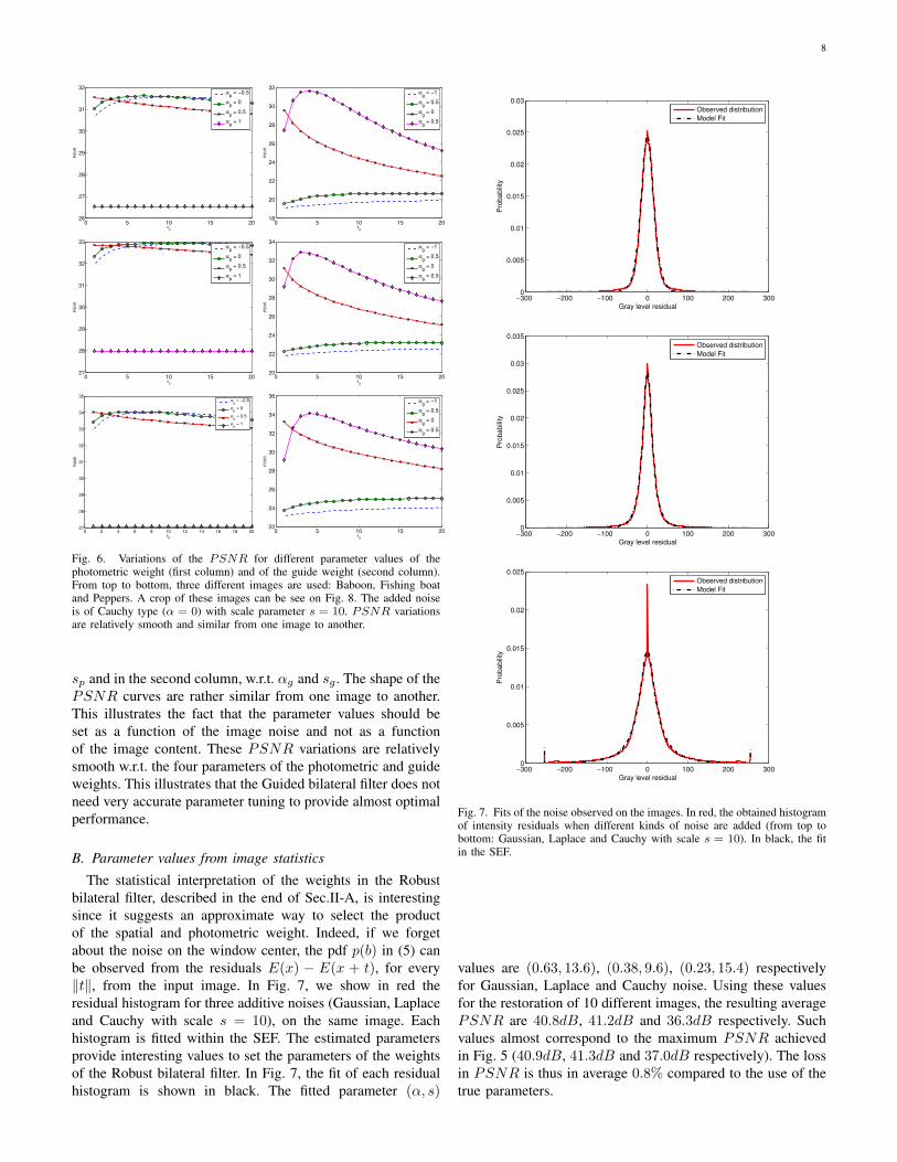
Fig. 6. Variations of the PSNR for different parameter values of thephotometric weight (first column) and of the guide weight (second column).From top to bottom, three different images are used: Baboon, Fishing boatand Peppers. A crop of these images can be see on Fig. 8. The added noiseis of Cauchy type (α = 0) with scale parameter s = 10. PSNR variationsare relatively smooth and similar from one image to another.
sp and in the second column, w.r.t. αg and sg . The shape of the
PSNR curves are rather similar from one image to another.
This illustrates the fact that the parameter values should be
set as a function of the image noise and not as a function
of the image content. These PSNR variations are relatively
smooth w.r.t. the four parameters of the photometric and guide
weights. This illustrates that the Guided bilateral filter does not
need very accurate parameter tuning to provide almost optimal
performance.
B. Parameter values from image statistics
The statistical interpretation of the weights in the Robust
bilateral filter, described in the end of Sec.II-A, is interesting
since it suggests an approximate way to select the product
of the spatial and photometric weight. Indeed, if we forget
about the noise on the window center, the pdf p(b) in (5) can
be observed from the residuals E(x) − E(x + t), for every
‖t‖, from the input image. In Fig. 7, we show in red the
residual histogram for three additive noises (Gaussian, Laplace
and Cauchy with scale s = 10), on the same image. Each
histogram is fitted within the SEF. The estimated parameters
provide interesting values to set the parameters of the weights
of the Robust bilateral filter. In Fig. 7, the fit of each residual
histogram is shown in black. The fitted parameter (α, s)
−300 −200 −100 0 100 200 3000
0.005
0.01
0.015
0.02
0.025
0.03
Gray level residual
Pro
ba
bili
ty
Observed distribution
Model Fit
−300 −200 −100 0 100 200 3000
0.005
0.01
0.015
0.02
0.025
0.03
0.035
Gray level residual
Pro
ba
bili
ty
Observed distribution
Model Fit
−300 −200 −100 0 100 200 3000
0.005
0.01
0.015
0.02
0.025
Gray level residual
Pro
ba
bili
ty
Observed distribution
Model Fit
Fig. 7. Fits of the noise observed on the images. In red, the obtained histogramof intensity residuals when different kinds of noise are added (from top tobottom: Gaussian, Laplace and Cauchy with scale s = 10). In black, the fitin the SEF.
values are (0.63, 13.6), (0.38, 9.6), (0.23, 15.4) respectively
for Gaussian, Laplace and Cauchy noise. Using these values
for the restoration of 10 different images, the resulting average
PSNR are 40.8dB, 41.2dB and 36.3dB respectively. Such
values almost correspond to the maximum PSNR achieved
in Fig. 5 (40.9dB, 41.3dB and 37.0dB respectively). The loss
in PSNR is thus in average 0.8% compared to the use of the
true parameters.
9
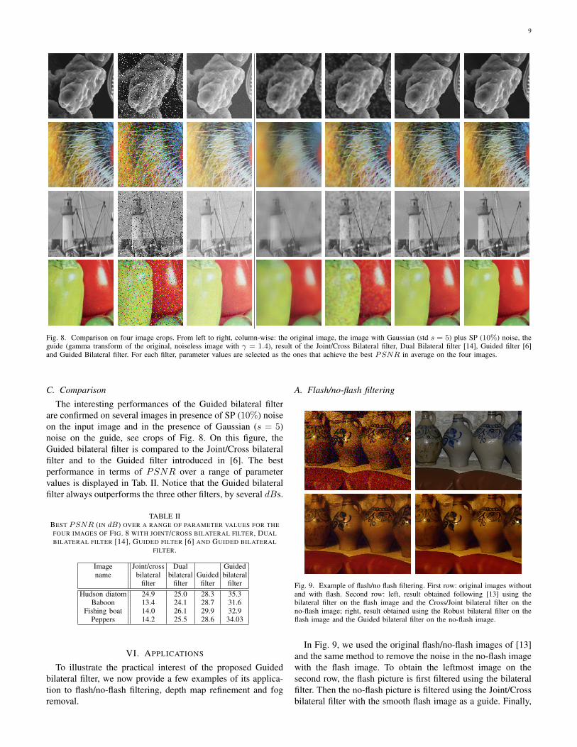
Fig. 8. Comparison on four image crops. From left to right, column-wise: the original image, the image with Gaussian (std s = 5) plus SP (10%) noise, theguide (gamma transform of the original, noiseless image with γ = 1.4), result of the Joint/Cross Bilateral filter, Dual Bilateral filter [14], Guided filter [6]and Guided Bilateral filter. For each filter, parameter values are selected as the ones that achieve the best PSNR in average on the four images.
C. Comparison
The interesting performances of the Guided bilateral filter
are confirmed on several images in presence of SP (10%) noise
on the input image and in the presence of Gaussian (s = 5)
noise on the guide, see crops of Fig. 8. On this figure, the
Guided bilateral filter is compared to the Joint/Cross bilateral
filter and to the Guided filter introduced in [6]. The best
performance in terms of PSNR over a range of parameter
values is displayed in Tab. II. Notice that the Guided bilateral
filter always outperforms the three other filters, by several dBs.
TABLE IIBEST PSNR (IN dB) OVER A RANGE OF PARAMETER VALUES FOR THE
FOUR IMAGES OF FIG. 8 WITH JOINT/CROSS BILATERAL FILTER, DUAL
BILATERAL FILTER [14], GUIDED FILTER [6] AND GUIDED BILATERAL
FILTER.
Image Joint/cross Dual Guidedname bilateral bilateral Guided bilateral
filter filter filter filter
Hudson diatom 24.9 25.0 28.3 35.3Baboon 13.4 24.1 28.7 31.6
Fishing boat 14.0 26.1 29.9 32.9Peppers 14.2 25.5 28.6 34.03
VI. APPLICATIONS
To illustrate the practical interest of the proposed Guided
bilateral filter, we now provide a few examples of its applica-
tion to flash/no-flash filtering, depth map refinement and fog
removal.
A. Flash/no-flash filtering
Fig. 9. Example of flash/no flash filtering. First row: original images withoutand with flash. Second row: left, result obtained following [13] using thebilateral filter on the flash image and the Cross/Joint bilateral filter on theno-flash image; right, result obtained using the Robust bilateral filter on theflash image and the Guided bilateral filter on the no-flash image.
In Fig. 9, we used the original flash/no-flash images of [13]
and the same method to remove the noise in the no-flash image
with the flash image. To obtain the leftmost image on the
second row, the flash picture is first filtered using the bilateral
filter. Then the no-flash picture is filtered using the Joint/Cross
bilateral filter with the smooth flash image as a guide. Finally,

10
the details of the flash image are introduced by multiplying
the previous result with the ratio of the flash image over the
smooth flash image. The rightmost image on the second row
of Fig. 9 is obtained by using the Robust bilateral filter with
parameters ws = 1, αg = 1, sg = 1, αp = −1, sp = 3instead of a bilateral filter, and using the Guided bilateral
filter with parameters ws = 1, αg = 0, sg = 10, αp = −1,
sp = 40 rather than a Joint/Cross bilateral filter. Due to the
robustness of both filters, the result is smoother, and noise
is entirely removed. Moreover, the specularities of the flash
image are less transferred onto the no-flash image compared
to the previous result.
B. Depth map refinement
Fig. 10. Example of depth map refinement. First row: left, original image ofthe stereo pair; right, disparity map obtained using a dense stereo reconstruc-tion algorithm. Second row: the refined disparity maps after filtering by theJoint/Cross bilateral filter (left) and after the Guided bilateral filter (right).
The Joint/Cross bilateral filter was used in [4] for depth map
refinement and interpolation using one of the original images
of the stereo pair as a guide. In Fig. 10, a disparity map is
obtained using a belief propagation algorithm on a Markov
random field model of the problem which was voluntarily
stopped before total convergence to save processing time.
Even if numerous outliers are present in the original image,
the refinement based on the Guided bilateral filter achieves
interesting results. To obtain these results, the GNC approach
was performed with parameters ws = 1, αg = 0, sg = 10,
αp = −1, sp = 40. The result obtained using the Joint/Cross
bilateral filter is less convincing, as shown on Fig. 10.
C. Single image fog removal
In this example, following [21], fog removal is performed in
two steps on a single image: first, atmospheric veil is estimated
from the color saturation (maximum over color channels for
each pixel) after median filtering; second, the veil is used
to remove the fog by reversing Koschmieder’s law, which
models fog effects. Between these two steps, the atmospheric
veil can be refined by applying the Guided bilateral filter on
the veil using the original color image as a guide. This extra
step allows better removing the fog between objects with thin
shapes such as leaves, as shown on Fig. 11. The parameters
of the Guided bilateral filter are ws = 1, αg = 0.5, sg = 30,
αp = 1, sp = 10 in this example.
VII. CONCLUSION
In this paper, we have reviewed the derivation of the
bilateral filter and several of its most efficient variants from
the point of view of robust statistics. In particular, we exper-
imentally shown that an IRLS implementation (called Robust
bilateral filter) is the only one that fully guarantees robust-
ness in the presence of noise and outliers. We proposed a
probabilistic interpretation of the weights that may be used
to unify the derivation of the filters and naturally leads to
the definition of a more generic filter, which we name the
Guided bilateral filter. The inputs of this filter are two images:
the image to be processed and the guide image. The Guided
bilateral filter requires four parameters if the guide is of
good quality or else five parameters. We provided insight
and recommendations for setting these parameters depending
on the input data. The proposed filter is iterative, hence we
provide a heuristic scheme, based on the Graduated Non
Convexity approach which helps converging towards a good
local minimum of the cost function, in a reduced number
of iterations. Experimentally, in terms of psnr, the Guided
bilateral filter outperforms the three other filters which take
into account a guide image. The proposed filter is robust to
outliers in the image to be processed but not to outliers in the
guide image. To overcome this limitation, simply we suggest
to pre-process the guide, using the Robust bilateral filter,
for instance. We show the interest of the proposed filter for
flash/no-flash filtering, depth map refinement and fog removal,
but many other applications could profit from its use, such as
visible/infrared filtering, sharpness enhancement, upsampling,
image editing, gray level image coloring, image recoloring, or
depth of field effect [22].
REFERENCES
[1] C. Tomasi and R. Manduchi, “Bilateral filtering for gray and colorimages,” in ICCV, 1998, pp. 839–846.
[2] B. Y. Zhang and J. P. Allebach, “Adaptive bilateral filter for sharp-ness enhancement and noise removal,” IEEE Trans. Image Processing,vol. 17, no. 5, pp. 664–678, May 2008.
[3] J. Kopf, M. F. Cohen, D. Lischinski, and M. Uyttendaele, “Joint bilateralupsampling,” ACM Trans. on Graphics, vol. 26, no. 3, July 2007.
[4] Q. X. Yang, R. G. Yang, J. Davis, and D. Nister, “Spatial-depth superresolution for range images,” in CVPR, 2007, pp. 1–8.
[5] E. A. Khan, E. Reinhard, R. Fleming, and H. Buelthoff, “Image-basedmaterial editing,” ACM Trans. on Graphics, vol. 25, no. 3, pp. 654–663,July 2006.
[6] K. He, J. Sun, and X. Tang, “Guided image filtering,” in European
Conference on Computer Vision (ECCV’10), Hersonissos, Crete, Greece,2010, pp. 1–14.
[7] S. Paris, P. Kornprobst, J. Tumblin, and F. Durand, “Bilateral filtering:Theory and applications,” Foundations and Trends R© in Computer
Graphics and Vision, vol. 4, no. 1, pp. 1–75, 2009.[8] M. Elad, “On the origin of the bilateral filter and ways to improve it,”
IEEE Trans. Image Processing, vol. 11, no. 10, pp. 1141–1151, Oct.2002.
[9] A. Buades, B. Coll, and J. M. Morel, “The staircasing effect inneighborhood filters and its solution,” IEEE Trans. Image Processing,vol. 15, no. 6, pp. 1499–1505, Jun. 2006.
[10] F. Durand and S. Paris, “A fast approximation of the bilateral filter usinga signal processing approach,” in ECCV, 2006, pp. IV: 568–580.

11
Fig. 11. Example of single image defogging. First column: original foggy images. Second column: fog removal using the fast median filter [21]. Thirdcolumn: fog removal using the Guided bilateral filter. Notice how halos produced by the median filter are removed with the Guided bilateral filter.
[11] B. Weiss, “Fast median and bilateral filtering,” ACM Trans. on Graphics,vol. 25, no. 3, pp. 519–526, July 2006.
[12] E. Eisemann and F. Durand, “Flash photography enhancement viaintrinsic relighting,” ACM Trans. on Graphics, vol. 23, no. 3, pp. 673–678, Aug. 2004.
[13] G. Petschnigg, R. Szeliski, M. Agrawala, M. Cohen, H. Hoppe, andK. Toyama, “Digital photography with flash and no-flash image pairs,”ACM Trans. on Graphics, vol. 23, no. 3, pp. 664–672, Aug. 2004.
[14] E. P. Bennett, J. L. Mason, and L. McMillan, “Multispectral bilateralvideo fusion,” IEEE Trans. Image Processing, vol. 16, no. 5, pp. 1185–1194, May 2007.
[15] S.-S. Ieng, J.-P. Tarel, and P. Charbonnier, “Modeling non-gaussian noisefor robust image analysis,” in Proceedings of International Conference
on Computer Vision Theory and Applications (VISAPP’07), Barcelona,Spain, 2007, pp. 183–190.
[16] J.-P. Tarel, S.-S. Ieng, and P. Charbonnier, “A constrained-optimizationbased half-quadratic algorithm for robustly fitting sets of linearlyparametrized curves,” Advances in Data Analysis and Classification,vol. 2, no. 3, pp. 227–239, 2008.
[17] P. Charbonnier, L. Blanc-Feraud, G. Aubert, and M. Barlaud, “Determin-istic edge-preserving regularization in computed imaging,” IEEE Trans.
Image Processing, vol. 6, no. 2, pp. 298–311, 1997.[18] J.-P. Tarel, S.-S. Ieng, and P. Charbonnier, “Using robust estimation
algorithms for tracking explicit curves,” in ECCV, vol. I, Copenhagen,Denmark, 2002, pp. 492–507.
[19] S. Geman and D. McClure, “Bayesian image analysis: an applicationto single photon emission tomography,” Proc. Statistical Computational
Section, Amer. Statistical Assoc., pp. 12–18, 1985.[20] A. Blake and A. Zisserman, Visual Reconstruction. Cambridge, MA:
MIT Press, 1987.[21] J.-P. Tarel and N. Hautiere, “Fast visibility restoration from a single color
or gray level image,” in ICCV, Kyoto, Japan, 2009, pp. 2201–2208.[22] E. S. L. Gastal and M. M. Oliveira, “Domain transform for edge-aware
image and video processing,” ACM Trans. Graph., vol. 30, no. 4, pp.69:1–69:12, Jul. 2011.
Laurent Caraffa received a M.S. degree in Com-puter Vision and Image Processing from the Univer-sity of Nice Sophia-Antipolis in 2010. He receivedhis PhD degree in Computer Science Paris VI-P.and M. Curie University in 2013 on stereo 3Dreconstruction taking into account bad weather con-ditions. From 2011, he is with the French instituteof science and technology for transport, developmentand networks (IFSTTAR).
Jean-Philippe Tarel graduated from the EcoleNationale des Ponts et Chaussees (ENPC), Paris,France (1991). He received his PhD degree in Ap-plied Mathematics from Paris IX-Dauphine Univer-sity in 1996. He was with the Institut National deRecherche en Informatique et Automatique (INRIA)from 1991 to 1996 and from 2001 to 2003. From1997 to 1998, he worked as a research associateat Brown University, USA. From 1999, he is aresearcher in the French institute of science andtechnology for transport, development and networks
(IFSTTAR and formerly LCPC), Paris, France. His research interests include3D reconstruction, pattern recognition and detection.
Pierre Charbonnier received the Ph.D. degree inelectrical engineering from the University of Nice-Sophia Antipolis, in 1994. He did a post-doc atthe Telecommunications and Remote Sensing Lab-oratory in Louvain-La-Neuve, Belgium in 1995-96.He is currently a Senior Researcher at the Cerema(center for expertise and engineering on risks, urbanand country planning, environment and mobility), inStrasbourg, France. He leads the ERA 27 (Cerema-IFSTTAR) research group. Since 2000, he is anexternal collaborator of the laboratory iCube (UMR
7357 CNRS-UDS). His research interests include inverse problems andregularization, classification and shape recognition (deformable models, robustestimation techniques) and computer vision.