ipe ii: monetary macroeconomics · 4.institutional analysis of monetary, fiscal and exchange rate...
TRANSCRIPT

IPE II: Monetary Macroeconomics
(Module MW25.3)
Prof. Dr. A. Freytag, PD Dr. M. Pasche
Friedrich Schiller University Jena
Work in progress! Bug report to: [email protected]
1

Outline:
1. Introduction
2. Exchange Rates and Current Account
2.1 Preliminaries2.2 Determinants of Exchange Rates2.3 Exchange Rates and Current Account Response
3. Monetary Macroeconomic Models
3.1 Overshooting Model (Dornbusch)3.2 New Keynesian Model
4. Institutional Analysis of Monetary, Fiscal and Exchange RatePolicy
4.1 Historical Exchange Rate Regimes4.2 Rule Binding and Discretionary Monetry Policy in an Open
Economy4.3 Rules, Independence, Credibility – the Problem of
Interdependence of Monetary and Fiscal Policy4.4 Governmental Debt, Inflation and Currency Crisis
2

5. Currency Crisis
5.1 Models of Currency Crisis5.2 Currency Crisis in a Monetary Union
Basic Literature:
I Cukierman, A.S. (1992), Central Bank Strategy, Creditibility andIndependence. Theory and Evidence. Cambridge/Mass. and London.The MIT Press.
I de Haan, J., Oosterloo, S., Schoenmaker, D. (2009), EuropeanFinancial Markets and Institutions. Cambridge: CambridgeUniversity Press:
3
I Fischer, S., Vegh, S., Vegh, C. (2002), Modern Hyper- and HighInflations. Journal of Economic Literature, Vol. XL, pp. 837-880.
I Hayek, F.A. von (1990), Denationalisation of Money – TheArgument Refined. Institute of Economic Affairs, Hobart PaperSpecial 70, London.
I Krugman, P.R., Obstfeld, M., Melitz, M. (2014), InternationalEconomics: Theory and Policy, 10th edition, Prentice Hall.
I MacDonald, R. (2007), Exchange Rate Economics: Theory andEvidence. London and New York: Routledge.
I Obstfeld, M., Rogoff, K. (1996), Foundations of InternationalMacroeconomics. Cambridge: MIT Press.
I White, L. (1999), The Theory of Monetary Institutions. Malden andOxford: Blackwell Publishers.
4

Time schedule (summer term 2018):
Week Tuesday Thursday
15 ch.1 (Freytag) –16 ch.2 (Pasche) –17 ch.2 (Pasche) –
18 –∗) –
19 ch.3 (Pasche) –∗)
20 ch.3 (Pasche) exercise (Pasche)21 ch.3 (Pasche) exercise (Pasche)22 ch.4 (Freytag) exercise (Pasche)23 ch.4 (Freytag) exercise (Pasche)24 ch.4 (Freytag)25 ch.4 (Freytag)26 ch.5 (Pasche)27 ch.5 (Pasche)28 ch.5 (Freytag) exercise (Pasche)
∗) public holiday
5

Type of course:
I Elective course in specialization areas “World Economy” and“Public Economics”
I 2 hours per week lecture, exercises up to 2 hours per week(see schedule); 6 ECTS
Examination:
I 60 min. endterm exam (100%)
6

1. Introduction – Goals of the lecture
Understanding exchange rates
I Exchange rates as price, adjustment parameter and policyvariable
I RER, effective ER, future ER
I What can policy obtain with a depreciation?
I What explains exchange rate fluctuations?
I Can central banks be effective on forex markets?
I How do fixed ER regimes work?
I History of ER regimes
7

1. Introduction – Goals of the lecture
US-Dollar per Euro since 2000 (Source: ECB)
8

1. Introduction – Goals of the lecture
What happened to the Rand? (Source: Bloomberg)
9

1. Introduction – Goals of the lecture
Source: ECB Monthly Bulletin 02/2018
10

1. Introduction – Goals of the lecture
Understanding the balance of payments
I The accounting mechanism
I Is a trade surplus a good thing?
I What about a bilateral deficit?
I Is China doing well with its enormous trade surplus?
I What is a sustainable deficit in the current account?
I Debt cycle
I What is a global imbalance?
11

1. Introduction – Goals of the lecture
Source: Freytag, A. (2008), That Chinese “juggernaut” –should Europe really
worry about its trade deficit with China?, ECIPE Policy Brief 2/2008, Brussels, p.5.
12

1. Introduction – Goals of the lecture
Source: IMF
13

1. Introduction – Goals of the lecture
Understanding the macroeconomics of open economies
I Interaction of forex markets with capital and goods markets
I Interaction of forex rates, interest rates and inflation
I Analysis of fiscal and monetary policy (depending on theexchange rate regime)
I Can interest rate policy of central banks be an effectivemeasure in an open economy?
14

1. Introduction – Goals of the lecture
Understanding the political economy of monetary policy
I Costs of inflation
I Basic monetary rules
I Rules vs. discretion: time consistency and economic policy
I Central bank independence
I Interdependence of monetary and fiscal policy: nohyperinflation without public debt crisis!
15

1. Introduction – Goals of the lecture
Source: ECB Economic Bulletin 02/2018
16

1. Introduction – Goals of the lecture
Source: ECB Economic Bulletin 02/2018
17

1. Introduction – Goals of the lecture
Reserves Composition
Source: IMF; http://data.imf.org/?sk=E6A5F467-C14B-4AA8-9F6D-5A09EC4E62A4
18

1. Introduction – Goals of the lecture
Understanding currency crisis
I Causes for currency crises
I Currency crisis by generation
I Role of speculation
I Early warning systems
19

1. Introduction – Goals of the lecture
Euroland
I Is Euroland an optimum currency area?
I What are the advantages of a common currency?
I Necessary conditions for stability
I Is the Euro crisis a currency crisis?
I Incentives in the SGP
20

1. Introduction – Goals of the lecture
Source: ECB Economic Bulletin 02/2017
21

1. Introduction – Goals of the lecture
Source: ECB Economic Bulletin 02/2017
22

1. Introduction – Goals of the lecture
Source: ECB Monthly Bulletin 02/2017
23

1. Introduction – Goals of the lecture
Target2 balances in the Euro area January 2018
Source: Statistia
24

2. Exchange Rates and Current Account
Literature:
* Krugman, P.R., Obstfeld, M., Melitz, M. (2014), InternationalEconomics: Theory and Policy, 10th ed., Prentice Hall.
I Obstfeld, M., Rogoff, K. (1996), Foundations of InternationalMacroeconomics. Cambridge: MIT Press.
I Krueger, A.O. (1983), Exchange-rate determination.Cambridge University Press.
I Gartner, M. (1993), Macroeconomics Under FlexibleExchange Rates. LSE Handbooks in Economics.
25

2. Exchange Rates and Current Account2.1 Preliminaries
I Exchange rate: Nominal price of a currency, expressed inunits of another currency
I Price notation:
ep =domestic currency
foreign currencye.g. ep = 0.8
[e
$
]I Quantity notation:
eq =foreign currency
domestic currencye.g. eq = 1.25
[$
e
]I Depreciation/devaluation of the domestic currency:
ep increases, eq decreases
I Appreciation/upvaluation of the domestic currency:ep decreases, eq increases
I Notation: If we use e without an index, then price notation
26

2.1 Preliminaries2.1 Preliminaries
I The exchange rate in price or quantity notation is a bilateralexchange rate (ER).
I In order to display the value of a currency compared to thecurrencies of n relevant trade partners, one can construct anindex called effective exchange rate:
eeff =n∑
i=1
giei with 0 < gi < 1,n∑
i=1
gi = 1
or
eeff =n∏
i=1
egii with 0 < gi < 1,
n∑i=1
gi = 1
with ei as the ER to the currency of country i .
I Weights gi adjusted according to what?
27

2. Exchange Rates and Current Account2.1 Preliminaries
I ER as defined above is a nominal variable (money price).
I Real exchange rate = exchange rate of goods, not currencies
er =p
p∗=
peep · p∗$
=
[e
domestic good
e$ ·
$foreign good
]=
[foreign good
domestic good
]I Real exchange rate tells how many foreign (imported) goods a
country receives for one unit of a domestic (exported) good.
I In the literature, sometimes the terms of trade (t.o.t.) aredefined as a synonym for the real exchange rate, sometimesthey are defined as the reciprocal value of the real exchangerate. This is pure convention! We use it as a synonym.
28

2. Exchange Rates and Current Account2.1 Preliminaries
I In case of tradable and non-tradable goods the real ER isgiven by
er =pT
p∗T(1)
where pT , p∗T are the price indices for domestic and foreign
traded or tradable goods.
The overall price level is then composed as
p = αpT + (1− α)pNT
with pNT as the price level of non-tradable goods.
29

2.1 Preliminaries2.1 Preliminaries
Is a depreciation of domestic currency “good”?
I One the one hand (elasticity approach):
ep ↑ ⇒ [Ex(ep)− Im(ep)] ↑ ⇒ Y ↑
if Marshall-Lerner condition holds true (discussed later).
I But on the other hand:
ep ↑ ⇒ er (t.o.t.) ↓
For a unit of domestic goods the country receives less foreigngoods = decrease of welfare.
I The first argument requires non-utilized production capacities,the second argument is based on a total competitiveequilibrium.
30

2.1 Preliminaries2.1 Preliminaries
Effect of depreciation:
export good
import good
t.o.t.=pEx/e0 · pIm
depreciation e1 > e0
export good relatively cheaper[ImEx
]↓
t.o.t.=pEx/e1 · pIm
welfare declines
31

2.1 Preliminaries2.1 Preliminaries
Forex Markets:
I Agents: Banks and other Financial Intermediaries, Firms,Central Bank, private traders.
I Each agent can act on the supply as well as on the demandside.
I Traded currencies are deposits, not cash.
I The majority of transactions are OTC, not via registered andregulated foreign exchange markets.
I The majority of transactions is processed electronically.
32

2.1 Preliminaries2.1 Preliminaries
I Spot Market: Trade contracts in t are executed immediatelyto the current spot rate et .
I Forward Markets: Contract in t to exchange (buy/sell)currencies in t + T to the forward rate et,T , where T are atleast 3 days, or 1, 2, 3, 6, 12 or more months.
This is typically done in order to reduce the risk of futureexchange rate changes (hedging).
33

2.1 Preliminaries2.1 Preliminaries
I Swap Market: Combination of spot and forward contract.
Swap rate: St,T =et,T−et
etwhere S > 0 is called “report” and
S < 0 is called “deport”.
Reasons: evtl. diverging expectations about future spot rates.
I Option Market: An option is the right to buy/sell a specificamount of a specific currency at a specific time point to aspecific exchange rate. This contract need not to be executed.
34

2.1 Preliminaries2.1 Preliminaries
Global foreign exchange market turnover by instrument
Average daily turnover in April, in billions of US dollars
Source: Bank of International Settlement, Triennial Central Bank Survey 2016
Instrument 1998 2001 2004 2007 2010 2013 2016Spot transactions 568 386 631 1.005 1.488 2.046 1.652Outright forwards 128 130 209 362 475 680 700Forex swaps 734 656 954 1.714 1.759 2.228 2.378Currency swaps 10 7 21 31 43 54 82Options/other 87 60 119 212 207 337 254Total 1.527 1.239 1.934 3.324 3.971 5.345 5.067
35

2.1 Preliminaries2.1 Preliminaries
Currency distribution of global foreign exchange market turnoverPercentage shares of daily average turnover in April.Each transaction involves two currencies, so that percentages will sum up to 200%.
Source: Bank of International Settlement, Triennial Central Bank Survey 2016
Currency 1998 2001 2004 2007 2010 2013 2016US dollar 86.8 89.9 88.0 85.6 84.9 87.0 87.6Euro ... 37.9 37.4 37.0 39.1 33.4 31.4Japanese yen 21.7 23.5 20.8 17.2 19.0 23.0 21.6Pound sterling 11.0 13.0 16.5 14.9 12.9 11.8 12.8Australian dollar 3.0 4.3 6.0 6.6 7.6 8.6 6.9Swiss franc 7.1 6.0 6.0 6.8 6.3 5.2 4.8Canadian dollar 3.5 4.5 4.2 4.3 5.3 4.6 5.1South African rand 0.4 0.9 0.7 0.9 0.7 1.1 1.0Chinese renminbi 0.0 0.0 0.1 0.5 0.9 2.2 4.0...
......
......
......
...Total 200 200 200 200 200 200 200
36

2.1 Preliminaries2.1 Preliminaries
Motives of agents on Forex markets:
I Purchasing and selling goods induces demand and supply ofcurrencies
I Capital transfers:I Providing and repaying credits in foreign currenciesI FDI: long-run investment in foreign assetsI Portfolio investment: short-run investments in foreign assets
I Arbitrage
I Speculation
I Hedging
I Central Bank interventions
37

2.1 Preliminaries2.1 Preliminaries
Arbitrage:
I Using existing differences in exchange rates at a time point.
I Simple arbitrage (example): Buying Dollar at ep in Frankfurtand selling it at the same time at e ′p > ep in New York. Bydoing so, the excess Dollar demand in Frankfurt and theexcess Dollar supply in New York will equalize the rates.
I Triangle arbitrage (example): Buying Dollar for Euro, buyingYen for Dollar, selling Yen for Euro if this is advantagous.
I Since transaction costs are low, Forex markets can beconsidered to be nearly “arbitrage free” (law of one price)
38

2.1 Preliminaries2.1 Preliminaries
Speculation:
I Using expected differences in exchange rates in a timeinterval.
I Spot market speculation:I without interest rate effects: E [et+1] > et
I with interest rate effects: (E [et+1]− et)/et > i − i∗
I Forward market speculation: Buying foreign currency to agiven forward rate if you expect that it is lower then thefuture spot rate: E [et+T ] > et,T .
39

2.1 Preliminaries2.1 Preliminaries
Effects of speculation:
I If underlying expectations contain valuable information aboutthe “fundamentals” of a currency, then a speculative agentwill buy a currency which is expected to be “undervalued”.This will help to adjust the price system to importantinformation which will enhance allocation efficiency. It mayhelp to smoothen ER fluctuations.
I If underlying expectations are not fundamentally justifiable,then speculation may induce self-fulfilling prophecies, leadingto bubbles and increased volatility. Note, that suchexpectations are not neccessarily “irrational” since they maybe fully consistent along the bubble path.
40

2.1 Preliminaries2.1 Preliminaries
Hedging:
If a contract contains future payments in a foreign currency, thenthe domestic agent faces an exchange rate risk. A risk averse agentwill try to avoid this risk.
I Contract contains payments in domestic currency (but then thetrade partner faces the same risk).
I Contract is accompanyied by a reverse forward contract. Example:exporter has future claims of 1000 Dollar in 3 months. Then he sellstoday the 1000 Dollar on the 3-months-forward market to the givenforward rate.
I Hedging (narrow sense): Trading the risk by an accompanying loan.Example: exporter has future claims of 1000 Dollar in 3 months. Hedemands a loan of 1000 Dollar to a rate of i0, changes it in Euro atet and invests it for 3 months with an interest rate i1 < i0. In 3months he receives 1000 Dollar from the export contract and repaysthe loan. The cost of risk avoidance are the difference i0 − i1.
41

2. Exchange Rates and Current Account2.2 Determinants of Exchange Rates
Outline:
2.2.1 Asset Market Perspective: ER and Interest Rates
2.2.2 Monetary Perspective: ER and Money Supply
2.2.3 Real Perspective: ER, Trade, and Purchasing Power Parity
2.2.4 Production, Income and ER
2.2.5 Expectations and Speculative Bubbles
42

2. Exchange Rates and Current Account2.2 Determinants of Exchange Rates2.2.1 Asset Market Perspective: ER and Interest Rates
I Investing financial wealth in domestic or foreign assets.Goal: return on investment
I We consider only one interest rate i , i∗
(“∗” denotes foreign country).
I Demand for foreign currency is determined byinterest rate differentials.
43

2. Exchange Rates and Current Account2.2 Determinants of Exchange Rates2.2.1 Asset Market Perspective: ER and Interest Rates
(Uncovered) interest rate parity:
I Invested capital is changed into foreign currency: K/et
I After the investment period the wealth is: (1 + i∗)K/et .
I Changing back into domestic currency at the expectedexchange rate: (1 + i∗)K/et · eexp
t+1.
44

2. Exchange Rates and Current Account2.2 Determinants of Exchange Rates2.2.1 Asset Market Perspective: ER and Interest Rates
I Due to arbitrage the returns of foreign and domestic investmentopportunities will be equalized:
(1 + i)K = (1 + i∗)K ·eexp
t+1
et
which leads to the uncovered interest rate parity (IRP):
1 + i
1 + i∗=
eexpt+1
et| − 1
1 + i
1 + i∗− 1 + i∗
1 + i∗=
eexpt+1
et− et
et
⇒ i − i∗
1 + i∗=
eexpt+1 − et
et≈ i − i∗
⇒ R∗ ≡ i∗ +eexp
t+1 − et
et≈ i
45

2. Exchange Rates and Current Account2.2 Determinants of Exchange Rates2.2.1 Asset Market Perspective: ER and Interest Rates
I Another notation using the approximation ln(1 + x) ≈ x :
i − i∗ ≈ ln eexpt+1 − ln et
Interest rates difference = expected change of ER.
I Example: eexpt+1 = 0.8, i∗ = 0.05
et R∗
0.75 0.12 (expected depreciation)0.8 0.05 (no change expected)
0.84 0.002 (expected appreciation)
46
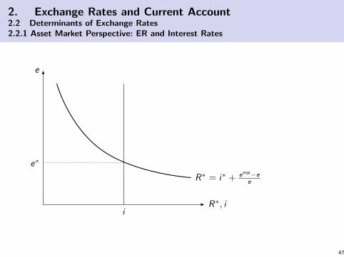
2. Exchange Rates and Current Account2.2 Determinants of Exchange Rates2.2.1 Asset Market Perspective: ER and Interest Rates
e
R∗, i
R∗ = i∗ + eexp−ee
i
e∗
47

2. Exchange Rates and Current Account2.2 Determinants of Exchange Rates2.2.1 Asset Market Perspective: ER and Interest Rates
(a) Expected depreciatione
R∗, ii
e∗1e∗2
(b) Increase of domestic interest ratee
R∗, ii1
e∗1
i2
e∗2
(c) Increase of foreign interest ratee
R∗, ii
e∗1
e∗2
48

2. Exchange Rates and Current Account2.2 Determinants of Exchange Rates2.2.1 Asset Market Perspective: ER and Interest Rates
Covered IRP:
I Avoiding the risk of exchange rate changes by making aforward contract.
I Risk-free no-arbitrage condition then reads
eT ,t − et
et= i − i∗ = swap rate
I If covered and uncovered IRP would hold true, then theforward rate equals the expected spot rate.
49

2. Exchange Rates and Current Account2.2 Determinants of Exchange Rates2.2.1 Asset Market Perspective: ER and Interest Rates
Limited IRP:
eexpt − et
et+ RP = i − i∗ with RP as risk premium
with risk aversion and/or imperfect substitutability of domestic andforeign investment opportunities.
Analogoulsy for limited covered IRP.
RP might be time-varying.
50

2. Exchange Rates and Current Account2.2 Determinants of Exchange Rates2.2.1 Asset Market Perspective: ER and Interest Rates
Forward Premium Puzzle:
I In case of rational expectations the expected future spot rateis identical with the forward rate (UIRP and CIRP hold true),otherwise we would have systematic arbitrage possibilities.
I An OLS test of
et+T︸︷︷︸spot
= α + β eT ,t︸︷︷︸forward
+εt+T
should give α = 0, β = 1 which is not the case.Moreover, εt+T is serially correlated.
I This implies that we cannot simply replace eexpt+T = et+T .
Therefore we cannot test directly the UIRP approach.
51

2. Exchange Rates and Current Account2.2 Determinants of Exchange Rates2.2.1 Asset Market Perspective: ER and Interest Rates
Testing IRP:
I Since we neither can observe expected ER nor rely on rationalexpectations, we use the covered IRP approach.
I Starting with the original no-arbitrage condition
(1 + it) = (1 + i∗t )eT ,t
et
Using logarithmic approximation ln(1 + x) ≈ x we have
i = i∗ + ln(eT ,t)− ln(et)
52

2. Exchange Rates and Current Account2.2 Determinants of Exchange Rates2.2.1 Asset Market Perspective: ER and Interest Rates
I OLS approach:
⇒ ln(eT ,t)− ln(et) = α + β(it − i∗t ) + εt
I Tested hypothesis of (covered) IRP:
α = 0, β = 1
I Moderate evidence for CIRP at least in times of not toovolatile markets (Monatsbericht Juni 2005, DeutscheBundesbank).
I Weak evidence for UIRP.
I General problem: Volatility of ER hard to explain.
53

2. Exchange Rates and Current Account2.2 Determinants of Exchange Rates2.2.2 Monetary Perspective: ER and Money Supply
Given the IRP, we can relate the money market and central bankpolicy to the exchange rate:
I Assume real money demandL(Y , i) with∂L/∂Y > 0, ∂L/∂i < 0
I Assume autonomously fixedreal money supply M/P.
I Equilibrium M/P = L(Y , i).
i
L, Mp
L(Y , i)
Mp
i∗
54

2. Exchange Rates and Current Account2.2 Determinants of Exchange Rates2.2.2 Monetary Perspective: ER and Money Supply
(a) Increased money supplye
R∗, i
Mp, L
UIRP
i1
e∗1
L(Y , i)Mp
M′
p
i2
e∗2
(b) Increased incomee
R∗, i
UIRP
Mp, L
i
e∗1
L(Y , i)Mp
L(Y ′, i)
i2
e∗2
55

2. Exchange Rates and Current Account2.2 Determinants of Exchange Rates2.2.3 Real Perspective: ER, Trade, and Purchasing Power Parity
I Exchange rates determine relative prices of domestic andforeign goods.
I Trade of goods influences supply and demand for currencies⇒ exchange rate
I Simplfying Assumptions:
I All goods are tradable.I All goods are homogenous.I No transaction and transportation costs.
⇒ Law of one price (no arbitrage condition)
56

2. Exchange Rates and Current Account2.2 Determinants of Exchange Rates2.2.3 Real Perspective: ER, Trade, and Purchasing Power Parity
Absolute purchasing power parity (PPP):
P = eP∗ ⇒ e =P
P∗
or in growth rates
wP = we + wP∗ ⇒ we = wP − wP∗
ER changes according to inflation differential.
57

2. Exchange Rates and Current Account2.2 Determinants of Exchange Rates2.2.3 Real Perspective: ER, Trade, and Purchasing Power Parity
I Objection: Not all goods are tradable.Assume the following decomposition of the price index:
P = αPT + (1− α)PN
P∗ = α∗P∗T + (1− α∗)P∗NLet β = PN/PT , β
∗ = P∗N/P∗T . Then
P = (α + (1− α)β)PT = γPT
P∗ = (α∗ + (1− α∗)β∗)P∗T = γ∗P∗T
I PPP holds true only for tradables:
e =PT
P∗T=
P
P∗γ∗
γ
or in growth rates:
we = (wP − wP∗) + (wγ∗ − wγ)
which is the relative PPP.
58

2. Exchange Rates and Current Account2.2 Determinants of Exchange Rates2.2.3 Real Perspective: ER, Trade, and Purchasing Power Parity
I If goods and price structure is stable, i.e.
wγ∗ = wγ = 0
then the result in growth rates is the same as in case ofabsolute PPP.
I The change of PT ,PN , α depends on the macroeconomicdevelopment of the open economy.
59

2. Exchange Rates and Current Account2.2 Determinants of Exchange Rates2.2.3 Real Perspective: ER, Trade, and Purchasing Power Parity
Structural change and emerging countries:
I Income is determined by labor productivity (among others). Itis reasonable that productivity differences accross countriesare more pronounced in the tradable good sector.
I Increase in the tradable good sector productivity leads tohigher wages in the economy, leading to higher costs (andprices PN) in the non-tradable good sector. Prices in thetradable good sector are determined on the world market andwill not be changed by productivity growth.
I Catching-up countries will therefore typically have a higherinflation rate (Balassa-Samuelson effect).
60

2. Exchange Rates and Current Account2.2 Determinants of Exchange Rates2.2.3 Real Perspective: ER, Trade, and Purchasing Power Parity
Balassa-Samuelson effect:
I Assume that prices are primarly determined by wages P = l/θ withl = wage rate and θ = labor productivity.
I Then we have wP = wl − wθ.
I There are two sectors N and T , but only one wage rate. Therefore
wPT− wPN
= wθN− wθT
I Inflation rate is composed as
wP = αwPN+ (1− α)wPT
= wPT+ α(wθN
− wθT)
and for two countries
wP∗ − wP = wP∗T− wPT︸ ︷︷ ︸
0 (PPP)
+α [(wθ∗T − wθ∗N )− (wθT− wθN
)]︸ ︷︷ ︸>0 (typically)
61

2. Exchange Rates and Current Account2.2 Determinants of Exchange Rates2.2.3 Real Perspective: ER, Trade, and Purchasing Power Parity
The real exchange rate under PPP:
er =PT
eP∗T
I If PPP holds true, PT = eP∗T , then er = 1.
I Example: BigMac index (www.economist.com).
62

2. Exchange Rates and Current Account2.2 Determinants of Exchange Rates2.2.3 Real Perspective: ER, Trade, and Purchasing Power Parity
Source: www.economist.com
63

2. Exchange Rates and Current Account2.2 Determinants of Exchange Rates2.2.3 Real Perspective: ER, Trade, and Purchasing Power Parity
With PPP we should expect that nominal ER adjust according toinflation differences so that real ER do not change!
Empirical evidence:
I Nominal and real ER are highly correlated.
I No evidence for absolute PPP. Evidence for PPP only in caseof very high inflation countries. Weak evidence for relativePPP.
I Weak/moderate evidence also when applying PPP to tradablegoods only.
I ER are much more volatile than could be expected by PPP orIRP.
64

2. Exchange Rates and Current Account2.2 Determinants of Exchange Rates2.2.3 Real Perspective: ER, Trade, and Purchasing Power Parity
Reasons for deviation from PPP:
I Short run price rigidities: Nominal shocks are translated intoreal shocks
I Transportation costs
I Trade barriers
I Imperfect markets: differentiated products, market power
I Not all goods are tradable, Balassa-Samuelson effect
I Different preferences ⇒ different consumption bundles ⇒different measurement of price index
65

2. Exchange Rates and Current Account2.2 Determinants of Exchange Rates2.2.4 Production, income and ER
A simple macroeconomic model of an open economy(Mundell-Fleming):
Y = C (Y ) + I (i) + Ex(Y ∗, e)− Im(Y , e) + A
M
P= L(Y , i)
Current account:
I Trade account X (Y ,Y ∗, e) = Ex(Y ∗, e)− Im(Y , e).
I Capital account B(i , i∗) = K Im(i , i∗)− KEx (i , i∗).
I Without interventions of the central bank (zero currencyaccount), we have:
X (Y ,Y ∗, e) = −B(i , i∗)
which is called ZZ curve.66

2. Exchange Rates and Current Account2.2 Determinants of Exchange Rates2.2.4 Production, income and ER
ZZ curve in (Y , i)-space:
X (Y ,Y ∗, e) = −B(i , i∗)
I Combination of (Y , i) above this curve: domestic interest rate“too high” for equilibrium ⇒ capital inflow, excess demandfor domestic currency ⇒ appreciation.
I Combination of (Y , i) below this curve: domestic interest rate“too low” for equilibrium ⇒ capital outflow, excess demandfor foreign currency ⇒ depreciation.
Slope of curve depends on capital market imperfection (perfectcapital market: horizontal curve).
67

2. Exchange Rates and Current Account2.2 Determinants of Exchange Rates2.2.4 Production, income and ER
Domestic country:
Y = C (Y ) + I (i) + X (Y ,Y ∗, e) + A
M
P= L(Y , i)
X (Y ,Y ∗, e) = −B(i , i∗)
Foreign country:
Y ∗ = C ∗(Y ∗) + I ∗(i∗) + X ∗(Y ∗,Y , e) + A∗
M∗
P∗= L∗(Y ∗, i∗)
X ∗(Y ∗,Y , e) = −B∗(i∗, i)Because X = −X ∗ and B = −B∗ the last equation is redundant.
System with 5 equations and 5 endogeneous variables(Y ,Y ∗, i , i∗, e).What happens if domestic demand (income) increases? 68

2. Exchange Rates and Current Account2.2 Determinants of Exchange Rates2.2.4 Production, income and ER
i
Y
IS
LM
ZZA
IS ′
B
A ↑
IS ′′
ZZ ′
e ↓
e ↓
C
69

2. Exchange Rates and Current Account2.2 Determinants of Exchange Rates2.2.4 Production, income and ER
Increased domestic autonomous demand:
I Domestic income and imports increase. Trade balancedecreases, demand for foreign currency increases.
I Domestic interest level increases, inducing more capitalinflows. This leads to increased demand for domestic currency.
I Increasing interest rates dampen positive income effect.
I We obtain a net excess demand for domestic currency →appreciation → dampening effect.
70

2. Exchange Rates and Current Account2.2 Determinants of Exchange Rates2.2.5 Expectations and Speculative Bubbles
Example of a simple bubble model:
I Uncovered IRP always holds true:
i − i∗ =E [et+1]− et
et= E [∆ ln e]
I Assume that there is a “fundamental” equilibrium level eI If realized ER differs from its equilibrium level, there is a
probability p that ER adapts to its equilibrium level (e − et).The rate of ER change is therefore (ln e − ln e).
I With probability (1− p) agents expect that the deviation fromthe equilibrium level increases with a constant rate (“bubblepath”): ∆ ln e. And with p the bubble will burst.
I Rational agents will account for both possible events andexpect
E [∆ ln e] = p(ln e − ln e) + (1− p)(∆ ln e)
71

2. Exchange Rates and Current Account2.2 Determinants of Exchange Rates2.2.5 Expectations and Speculative Bubbles
I Employing IRP gives
i − i∗ = p(ln e − ln e) + (1− p)(∆ ln e)
I Solving to ∆ ln e gives
∆ ln e =1
1− p(i − i∗) +
p
1− p(ln e − ln e)
I This means that the increase of the bubble is larger, the largerthe deviation from the equilibrium level is already, i.e. thebubble path is exponential until the bubble bursts.
I Note, that expectations are always rational, even on thebubble path!
72
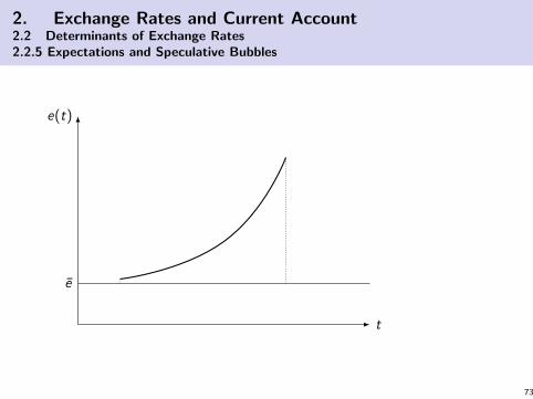
2. Exchange Rates and Current Account2.2 Determinants of Exchange Rates2.2.5 Expectations and Speculative Bubbles
e(t)
t
e
73

2. Exchange Rates and Current Account2.2 Determinants of Exchange Rates2.2.5 Expectations and Speculative Bubbles
Problems of this simple model:
I Initial creation and burst of the bubble are not explained.
I Exogenous probabilities of burst.
I ER bubbles should influence interest rates and prices (here:given as parameters, not endogenous variables)
I Difficult to prove empirical evidence.
Similar approach: herding behavior
74

2. Exchange Rates and Current Account2.3 Exchange Rates and Current Account Response
Structure of the balance of payments:
1. Current account
1.1 Trade account1.2 Services account1.3 Direct income transfers1.4 Other transfers
2. Capital account
2.1 FDI account2.2 Account of financial assets2.3 Other capital transfers
3. Currency account
4. Statistically not assignable transactions
75

2. Exchange Rates and Current Account2.3 Exchange Rates and Current Account Response
Since each accounting record has two entries, all net total of theaccounts have to add up to zero (closed system).
I An exporter sells goods and receives foreign currency:
current accountEx = 100
NX = 100
capital accountKEx = 100
B = −100
I A domestic bank sells foreign currency to the central bank:
capital accountKEx = −100
B = 100
currency account∆C = 100
∆R = 100
76

2. Exchange Rates and Current Account2.3 Exchange Rates and Current Account Response
I An importer buys foreign goods and the foreign firm has openclaims:
current accountIm = 100
NX = −100
capital accountK Im = 100
B = 100
I An investor buys a foreign firm and pays with foreign currency:
capital accountK Im
long = 100
K Imshort = −100
77

2. Exchange Rates and Current Account2.3 Exchange Rates and Current Account Response
I Net balances:I Current account NX = Ex − Im (net export)I Capital account B = K Im − KEx (net capital import)I Currency account ∆R = NX + B (net change of foreign
reserve stock)
I In case of flexible exchange rates, the central bank has not topurchase/sell foreign currencies: ∆R = 0⇒ NX = −B
I Capital and current account are then like a “mirror”.
78

2. Exchange Rates and Current Account2.3 Exchange Rates and Current Account Response
I From macroeconomic accounting we have
Y = C + I + Ex − Im
Y − C − I = S − I = Ex − Im = NX
⇒ S − I = ∆R − B = NX
and for ∆R = 0 we have
S − I = KEx − K Im
I Positive net exports mean that domestic savings exceeddomestic investments. There are more domestic saversinvesting abroad than vice versa = net capital outflow.
I How does the current account respond to changes of theexchange rate?
79

2. Exchange Rates and Current Account2.3 Exchange Rates and Current Account Response
The Marshall-Lerner condition:
I Depreciation enables export firms to charge a lower price inforeign currency. The sold quantity as well as the price indomestic currency and henceforth Ex will increase.
I The imports will become more expensive in domestic currencyso that the imported quantity will decrease. Therefore wehave countervailing effects so that the resulting effect on thevalue Im is ambigous. Hence, the effect on NX is ambigous.
I Therefore, the intuitive effect that NX increases in case ofdepreciation (“normal” response) holds true only undercertain conditions.
I Note, that an increase of NX has no normative imlpications.
80

2. Exchange Rates and Current Account2.3 Exchange Rates and Current Account Response
NX (e) = Ex(e)− Im∗(e)e
dNX
de=
dEx
de− dIm∗
dee − Im∗
We say a “normal” reaction is dNX/de > 0 and presume abalanced trade Ex = Im∗e ⇒ Im∗ = Ex/e:
0 <dEx
de
e
ExIm∗ − dIm∗
de
e
Im∗Im∗ − Im∗
0 <dEx
de
e
Ex− dIm∗
de
e
Im∗− 1
1 < ηEx − ηIm∗
81

2. Exchange Rates and Current Account2.3 Exchange Rates and Current Account Response
I In the short-run, demand and supply side in export andimport markets cannot respond immediately to ER changes(e.g. existing contracts).
⇒ If e increases, then it takes some time until Im∗(e) decreases.
I But the value of imports in domestic currency e · ¯Im∗
willincreases immediately.
I The resulting effect is that in the short-run we may observe asharp fall of NX before the “normal reaction” takes place.The time-path is characterized by the “J-curve effect”.
82

2. Exchange Rates and Current Account2.3 Exchange Rates and Current Account Response
NX
t
depreciation shock
83

2. Exchange Rates and Current Account2.3 Exchange Rates and Current Account Response
I We have only analyzed how exogenous changes of ER affectsceteris paribus the trade balance.
I We have seen, however, that trade balance corresponds withcapital balance.
I Trade depends on prices, capital flows depend on interestrates, both are determining the nominal exchange rate.
I In equilibrium, individual plans which determine B and NXhave to be consistent – which implies a certain real exchangerate.
I Such an equilibrium does not neccessarily imply balancedtrade and capital accounts.
84

2. Exchange Rates and Current Account2.3 Exchange Rates and Current Account Response
Capital flows as an intertemporal decision problem:
I For capital accumulation we need savings and production ofinvestment goods.
I This requires an intertemporal decision: Partial waive forconsumption today enables larger output and consumptiontomorrow.
I Transfer of capital is not physical capital but financial capital. It canbe used in the foreign country either for additional consumption oradditional investment.
I Home country has then claims on the future GDP of the foreigncountry: The interest rate payments to the home country has to beraised from the foreign’s future GDP.
I For the domestic intertemporal consumption/saving decision, the(real) interest rates r , r∗ play an important role. With a given worldcapital market interest rate r = r∗ and given intertemporalpreferences, the net exports and the trade balance are implicetlydetermined (see below).
85

2. Exchange Rates and Current Account2.3 Exchange Rates and Current Account Response
Intertemporal calculus:
I 2 periods, only one good that can either be consumed orinvested
I perfect capital market with one interest rate for lending andborrowing
I Intertemporal budget constraint with lending/borrowing:
Ct+1 = Yt+1 + (1 + r)(Yt − Ct)
⇒ Ct +1
1 + rCt+1 = Yt +
1
1 + rYt+1
86

2. Exchange Rates and Current Account2.3 Exchange Rates and Current Account Response
I Consumers maximize the net present utility
U = U(Ct) +1
1 + ρU(Ct+1)
with ρ as the intertemporal discount rate (reflectingpreference for the presence or “impatience”). They have tomaximize utility conditional to the intertemporal budgetconstraint (DD in the following figure).
87

2. Exchange Rates and Current Account2.3 Exchange Rates and Current Account Response
Yt+1,Ct+1
Yt ,Ct
45
PYt+1
Yt
D
D
determined by r
CCt+1
Ct
A
(a)
(a) Borrowing in t (Import)
(b)
(b) Repaying in t + 1 (Export)
88

2. Exchange Rates and Current Account2.3 Exchange Rates and Current Account Response
I In t the households consume more than it is produced= positive net imports Imt
= negative trade balance AC (= positive capital balance).The consumption is partially financed by foreign savings (debt)
I In t + 1 the debt is repaid including interest rate: AP,implying a positive trade balance (= negative capital balance).
I Both imbalances in t and t + 1 reflect optimal behavior, notdisequilibrium.
89

2. Exchange Rates and Current Account2.3 Exchange Rates and Current Account Response
I Now consider that Y can not only be consumed but also beinvested.
I Investment leads to capital accumulation. Thus theproduction frontier shifts and we have
Yt+1 = Yt + F (It)
with F (·) as the production effect of investments andF ′ > 0,F ′′ < 0
I Saving and investment therefore lead to an intertemporalproduction frontier (RP in the following graphic).
90

2. Exchange Rates and Current Account2.3 Exchange Rates and Current Account Response
I The calculus of an investor is whether to invest into thephysical project It or to invest the funds at the world capitalmarket at the rate r . The returns from investment F (It) aretherefore discounted with 1/(1 + r).
I Profit maximization gives
maxItπ =
1
1 + rF (It)− It
FOC ⇒ dF
dIt= 1 + r
which is the tangential point Q at the intertemporalproduction frontier RP.
I Due to the increased production in t + 1 the intertemporalbudget constraint shifts to D ′D ′.
I The same calculus for intertemporal consumption is applied tothe new constraint. The achievable utility is higher thanbefore.
91

2. Exchange Rates and Current Account2.3 Exchange Rates and Current Account Response
Yt+1,Ct+1
Yt ,Ct
45
P
Yt
D
D
R
D’
D’
QYt+1
It
shift of budget constraint
92

2. Exchange Rates and Current Account2.3 Exchange Rates and Current Account Response
Yt+1,Ct+1
Yt ,Ct
45
Yt
D
D
R
D’
D’
QYt+1
It
CCt+1
Ct
Imt
Ext+1
A B
93

2. Exchange Rates and Current Account2.3 Exchange Rates and Current Account Response
The complete result of intertemporal consumtpion and investmentdecisions:
I In t we have a negative trade balance (positive capitalbalance) AC , and investment AB.
I In t + 1 the foreign debt is repaid inclduing interest paymentsAQ which implies a positive trade balance.
I Borrowing and repaying capital is indirectly borrowing andregiving goods.
94

2. Exchange Rates and Current Account2.3 Exchange Rates and Current Account Response
Consider two countries with different investment opportunities anddifferent time preferences:
I An optimal positive trade balance in t in country 1 implies anoptimal negative trade balance in t in country 2, and viceversa in t + 1.
I Given the time preferences and different returns oninvestments (different intertemporal production frontiers), theoptimal plans for consumption and investment (andhenceforth exports and imports) must be consistent.
I The world market interest rate r adjusts so that intertemporalplans of both countries are coordinated.
95

2. Exchange Rates and Current Account2.3 Exchange Rates and Current Account Response
Yt+1, Ct+1
Yt , Ct
45
Yt
Country 1
−(1 + r)
Yt+1
ItCtExt
Imt+1
Yt+1, Ct+1
Yt , Ct
45
Yt
Country 2
−(1 + r)
Yt+1
It
Ct
Ext+1
Imt
Left side: low marginal productivity of It , patient consumersRight side: large marginal productivity of It , less patient consumers
96

2. Exchange Rates and Current Account2.3 Exchange Rates and Current Account Response
Empirical picture – UNCTAD World Investment Report 2014:
I FDI outflow 2013:I Developed countries: 899 billion USDI Developing and emerging countries: 553 billion USD
I FDI inflow 2013:I Developed countries: 566 billion USDI Developing and emerging countries: 886 billion USD
I In former decades these net flows from developed todeveloping countries had a much lower relative value....
I ... and national saving and investment rates are highlycorrelated (Feldstein-Horioka puzzle).
Possible reasons:
Other influences on savings, investments, cross-border flow ofcapital: uncertainty about economic and political development;quality of institutions (rule of law, corruption; enforcement ofproperty rights). 97

2. Exchange Rates and Current Account2.3 Exchange Rates and Current Account Response
The “debt cycle”:
I In a n-period model or in a continous time model, theintertemporal problem will first create increasing capitalinflows (debt accumulation), and in later periods net capitaloutflows (repaying debt), creating a “cycle” in trade andcapital net positions.
I There is some empirical evidence that such debt cyclesoccured (e.g. USA, South Africa, see the slide in the“Introduction”)
98

2. Exchange Rates and Current Account2.3 Exchange Rates and Current Account Response
Relation to ER:
I The intertemporal calculus implies that Ex − Im and S − I isplanned simultanously.
I The export/import plans of the country must be consistentwith the plans of the other country (or “rest of the world”).There exists an er = P/eP∗ where plans are consistent.
I The same holds true for planned S − I . The saving/investmentplans of both countries are coordinated by interest rates.
I Therefore the equilibrium exchange rate is implicitlydetermined by the intertemporal plans, and depends onprice differentials, interest rate differentials, and time prefencerates.
99

3. Monetary Macroeconomic Models
Outline:
3.1 Overshooting Model (Dornbusch)
3.2 (New) Keynesian Model
Literature:
I Krugman, P.R., Obstfeld, M., Melitz, M. (2014), InternationalEconomics: Theory and Policy, 10th edition, Prentice Hall.
I Rogoff, K. (2002), Dornbusch’s Overshooting Model afterTwenty-Five Years. IMF Staff Papers, Vol. 49, IMF Annual ResearchConference (2002), pp. 1-
I Dornbusch, R. (1976), Expectations and Exchange Rate Dynamics.Journal of Political Economy 84 (6), 1161–1176.
100

3. Monetary Macroeconomic Models3.1 Overshooting Model
Model by R. Dornbusch (1976):
I Slow goods market, fast capital market
I Short run: uncovered interest rate partity, fixed prices
I Long run: flexible prices, purchasing power parityI Analysing the impact of monetary shocks:
I If prices are flexible, nominal shocks in money supply inducenominal price increase, but real variables, including realexchange rate, are unaffected.
I With short-run rigid prices, the nominal shock has real effects;interest rate decreases and currency depreciates.
I When prices adapt to the new equilibrium level, investorsexpect appreciation.
I In the new equilibrium real interest rate and real exchange rateare on their initial levels. Nominal exchange rate has decreasedcompared to overshooting level.
101

3. Monetary Macroeconomic Models3.1 Overshooting Model
Notation:
y = lnY log incomem = lnM log nominal money supplyp = lnP log price level
e log exchange rateη > 0 income elasticity of money demandλ > 0 semi interest rate elasticity of money demand
102

3. Monetary Macroeconomic Models3.1 Overshooting Model
I From equilibrium condition for the money market we have
m − p = ηy − λi (2)
I Interest rate parity on the capital market is given by:
E [∆e] = i − i∗ ⇒ i = E [∆e] + i∗ (3)
I Expectations are given by
E [∆e] = θ(e − e) (4)
where e is determined by the PPP.I Inserting (4) and (3) into (2) gives the short run equilibrium
on money and capital market:
m = p + ηy − λ(θ(e − e) + i∗) (5)
⇒ p = λ(i∗ + θ(e − e))− ηy + m (SRE)
103

3. Monetary Macroeconomic Models3.1 Overshooting Model
I The relative PPP holds in the long run:
e = p − p∗ + Z (LRE)
I Before we analyze the interplay between (SRE) and (LRE) welook what happens with the short-run equation (5) in thelong-run: we replace p = p and consider e = e so that weobtain
m = p + ηy − λi∗ (6)
I Equalizing (5) and (6) and rearranging gives
e = e +1
λθ(p − p)
104

3. Monetary Macroeconomic Models3.1 Overshooting Model
Result:
I If the long-run price level p and henceforth the long-runequilibrium exchange rate e increase due to the nominalshock, then the short-run exchange rate e increases sharply ifprices are rigid.
I If then the price level p increases in time, the difference inbrackets become smaller so that the new exchange rateapproaches its new equilibrium level “from above”.
Graphic:
Recall that (SRE) shifts in case of a monetary shock:
SRE1 : p = λ(i∗ + θ(e1 − e))− ηy + m1
SRE2 : p = λ(i∗ + θ(e2 − e))− ηy + m2
105

3. Monetary Macroeconomic Models3.1 Overshooting Model
p
e
LRE
45 SRE0
p1
e1
SRE1
e
fast
p2
e2
slow
106
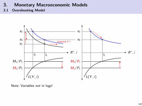
3. Monetary Macroeconomic Models3.1 Overshooting Model
R∗, i
L(Y , i)
M1/P1
i1
e1
M2/P1
expected e ↑
e2
i2
e3
R∗, i
L(Y , i)
M2/P1
e2
M2/P2
i1
e3
Note: Variables not in logs!
107

3. Monetary Macroeconomic Models3.1 Overshooting Model
money volume
time
interest rate
time
price level
time
exchange rate
time
108

3. Monetary Macroeconomic Models3.1 Overshooting Model
A dynamic model (discrete time version):
Assumptions:
I Long run equilibrium output y
I Foreign price level p∗ = 0 normalized to zero
I No interest rate dependency of demand (IS curve)
I IS curve: yt − y = b(et + p∗ − pt)
I LM curve: mt − pt = yt − βitI Interest rate partity : E [et+1 − et ] = it − i∗
I Rational expectations: E [et+1 − et ] = et+1 − et
I Phillips curve (price rigidity): pt+1 − pt = δ(yt − y)
109

3. Monetary Macroeconomic Models3.1 Overshooting Model
I From IS curve and Phillips curve we obtain
∆p = pt+1 − pt = δb(et − pt) (7)
I From LM curve and IRP we obtain
∆e = et+1 − et =1
β[yt −mt ]− i∗ +
1
βpt (8)
I The steady state is characterized by ∆p = ∆e = 0 andhenceforth it = i∗, yt = y , et = pt .
I In the steady state, (8) gives
et = pt = mt − y + βi∗
and therefore long-run neutrality of money:dp/dm = de/dm = 1, i.e. nominal variables are determined bymoney.
110

3. Monetary Macroeconomic Models3.1 Overshooting Model
e
p
∆e = 0
∆p = 0
111

3. Monetary Macroeconomic Models3.1 Overshooting Model
Disequilibrium:
I We have ∆e < 0 for pt < pss and vice versa.
I We have ∆p > 0 for et > pt and vice versa.
Graphical analysis:
I The ∆e = 0- and ∆p = 0-lines are isoclines. Theirintersection point characterizes the steady state.
I The arrows denote the dynamic motions as mentioned above.
I There exists only one stable path to the equilibrium(“saddle path”).
I Along this saddle path we have rational expectations.Different expectation hypothesis may eventually not lead to astable adaption path towards equilibrium.
112

3. Monetary Macroeconomic Models3.1 Overshooting Model
e
p
∆p = 0
p1
∆e = 0
e1
p1
∆e = 0
p2
∆e = 0
saddle path
e2
113

3. Monetary Macroeconomic Models3.1 Overshooting Model
Overshooting:
I With ∆m > 0 we have in the long run ∆p = ∆m. Theisocline ∆e = 0 shifts to the right.
I Starting from the initial equilibrium, the exchange rate“shoots up” to the saddle path.
I Then the price level and exchange rate move along the saddlepath to the new equilibrium.
Remark:
I There are different versions of the basic Dornbusch model,including e.g. continous time versions, and goods marketswith interest rate dependent investment, taxation etc..
114

3. Monetary Macroeconomic Models3.2 (New) Keynesian Model
Outline:
(a) Standard Keynesian Model of an Open Economy
Mankiw, N.G. (2010), Macroeconomics. 7th ed., Worth Publishers.
Krugman, P.R., Obstfeld, M., Melitz, M. (2014), International
Economics: Theory and Policy, 10th edition, Prentice Hall.
(b) New Consensus Models: Closed Economy
Carlin, W., Soskice, D. (2015), Macroeconomics. Institutions,
Instability, and the Financial System. Oxford University Press.
(c) New Consensus Models: Open Economy
Bofinger, P., Mayer, E., Wollmershauser, T. (2006), The BMWModel: A New Framework for Teaching Monetary Economics.Journal of Economic Education 37(1), 98-117.
Bofinger, P., Mayer, E., Wollmershauser, T. (2009), Teaching New
Keynesian Open Economy Macroeconomics at the Intermediate
Level. Journal of Economic Education 40(1), 80-101.
115

3. Monetary Macroeconomic Models3.2 (New) Keynesian Model
(a) Standard Keynesian Model of an Open Economy(Keynes-Mundell-Fleming model)
Y = C (Y ) + G + I (i) + NX (Y ,Y f , τ) (IS)
M
P= L(Y , i) (LM)
NX (Y ,Y f , τ) = −B(i , i f ) (ZZ)
where τ = eP f /P are the terms of trade.
I Assumption: Marshall-Lerner condition holds true.
I In case of fixed prices, τ can be replaced by e.
116

3. Monetary Macroeconomic Models3.2 (New) Keynesian Model
ZZ curve:NX (Y ,Y f , e) = −B(i , i f )
I Goods exporters and capital importers demand domesticcurrency.
I Goods importers and capital exporters demand foreigncurrency.
I With an equilibrium exchange rate e planned NX and planned−B are identical.
I Various combinations of (Y , i) with a given e lead to foreignexchange market equilibrium.
117

3. Monetary Macroeconomic Models3.2 (New) Keynesian Model
i
Y
IS
LM
ZZ
Above ZZ: appreciation presuure (e ↓)Below ZZ: depreciation pressure (e ↑)
118

3. Monetary Macroeconomic Models3.2 (New) Keynesian Model
Various cases in this model framework.....
Perfect versus imperfect capital markets:
I Imperfect: domestic and foreign currency are not perfectsubstitutes ⇒ IRP does not hold perfectly, i.e. there couldexist interest rate differences i 6= i f in equilibrium
⇒ upwards sloped ZZ curve
I Perfect: IRP holds: E [∆e] = i − i f = 0 in equilibrium. In caseof a small country: i f is a given fixed parameter.
⇒ horizontal ZZ curve
119

3. Monetary Macroeconomic Models3.2 (New) Keynesian Model
Small country versus large country:
I Small country: no effect on the “rest of the world”⇒ i f and Y f are given.
I Large country: various additional feedback mechanisms!
⇒ Since Im = Ex f , an increase of domestic imports affectsforeign income Y f which again stimulates domestic exports.
⇒ This has an effect on foreign inrterest rate i f . Both has animpact on the exchange rate e.
120

3. Monetary Macroeconomic Models3.2 (New) Keynesian Model
Flexible versus fixed exchange rate regime:
I Flexible ER: e is an endogenous variable (like Y and i) in thesystem of equations IS-LM-ZZ.; autonomous monetary policyis possible.
I Fixed ER: e = e is exogenously given, Central Bank (CB) hasto stabilize e by intervention ∆R 6= 0.
M + ∆R
P= L(y , i)
I Pressure on the exchange rate (intersection of IS and LM isnot on ZZ curve) induces a shift of LM.
I In case of a large country: Buying reserves = reducing foreignmoney supply in the private sector.
121

3. Monetary Macroeconomic Models3.2 (New) Keynesian Model
Fixed versus flexible prices
I Fixed prices: P = P and P f = P f (price rigidity).
I Flexible prices: modelling the supply side where expansion ofY is possible only with increasing P (short-/long-run Phillipscurve)
I Additional feedback mechanisms:I Effect on real money supply M/P = shift of LM curve.I Effect on terms of trade τ = shift of IS and ZZ curve.
122

3. Monetary Macroeconomic Models3.2 (New) Keynesian Model
Example I:
I small country
I fixed prices
I perfect capital markets
I flexible exchange rates
123

3. Monetary Macroeconomic Models3.2 (New) Keynesian Model
Monetary Policyi
Y
IS
LM
ZZA
LM’
M ↑
B
Point B: depreciation induced
IS ′
e ↓
C
Fiscal Policyi
Y
IS
LM
ZZA
IS ′
G ↑
B
Point B: appreciation induced
IS ′′
C
e ↑
124

3. Monetary Macroeconomic Models3.2 (New) Keynesian Model
I Monetary policy is very effective but not due a decrease of ibut due to an induced depreciation which stimulates thegoods market.
I Fiscal policy is ineffective because the induced appreciationcrowds out the stimulus completely.
125

3. Monetary Macroeconomic Models3.2 (New) Keynesian Model
Example II:
I small country
I fixed prices
I perfect capital markets
I fixed exchange rates
126

3. Monetary Macroeconomic Models3.2 (New) Keynesian Model
Monetary Policyi
Y
IS
LM
ZZA
LM’
M ↑
B
Point B: depreciation pressure⇒ CB must sell reserves
LM ′′
C
M ↓
Fiscal Policyi
Y
IS
LM
ZZA
IS ′
G ↑
B
Point B: appreciation pressure⇒ CB must buy reserves
LM’
M ↑
C
127

3. Monetary Macroeconomic Models3.2 (New) Keynesian Model
I Monetary policy is ineffective because it induces adepreciation which has to be offset by selling reserves (Mdeclines).
I Fiscal policy is very effective because it induces anappreciation which “forces” the central bank to buy reserveswhich means that monetary policy has to be expansive, too.(Not really independent CB.)
128

3. Monetary Macroeconomic Models3.2 (New) Keynesian Model
Example III:
I small country
I fixed prices
I imperfect capital markets
I flexible exchange rates
129

3. Monetary Macroeconomic Models3.2 (New) Keynesian Model
Fiscal policy:
i
Y
IS
LM
ZZA
IS ′
B
A ↑
IS ′′
ZZ ′
e ↓
e ↓
C
130

3. Monetary Macroeconomic Models3.2 (New) Keynesian Model
I Fiscal policy works like in the standard IS-LM model except foran additional (negative) feedback from induced appreciation.
I Crowding-out effect because of higher interest rate andappreciation ⇒ low fiscal multipliers.
131

3. Monetary Macroeconomic Models3.2 (New) Keynesian Model
Excourse: supply side – flexible prices
I We confine to a closed economy!
I If prices are seen as flexible, we can solve LM to i and plug it intothe IS curve in order to establish a negative relationship between Yand P (aggregated demand curve, AD)
I In addition, we have to model the supply side (AS curve) so thatprice level is determined endogenously.
132

3. Monetary Macroeconomic Models3.2 (New) Keynesian Model
I Wage bargaining: Nominal wage level is determinedaccording to the expected price level and the unemploymentrate u. A lower u implies higher bargaining power for theworkers:
w = Pe f (u), withdf
du< 0 (9)
I Price setting of firms: Since labor is the unique variableinput factor, wages w determine the marginal cost. Allowingfor imperfect markets, the price P is set with a certainmarkup on the marginal cost:
P = (1 + µ)w (10)
133

3. Monetary Macroeconomic Models3.2 (New) Keynesian Model
Determining the “natural rate of unemployment”:
I In the long run expected and realized price levels are equal:Pe = P.
I From (9) and (10) we have
w
Pe= f (u) (11)
w
P=
1
1 + µ(12)
I In the long run expected and realized price levels are equal:Pe = P. Replacing this in (11) and equalizing both equations,we obtain the natural unemployment rateun = f −1(1/(1 + µ)).
134

3. Monetary Macroeconomic Models3.2 (New) Keynesian Model
From unemployment to production (income):
I The unemployment rate u is defined by u = (L− N)/L(with L = labor force, N =employed workers).
I Assume a fixed labor productivity Y /N = 1/η ⇒ N = ηY .Then we have
u = 1− ηY
L(13)
I Inserting wage bargaining equation (9) into the pricedetermination (10) and substituting u by (13) we have theshort run aggregated supply function
P = Pe(1 + µ)f
(1− ηY
L
)(14)
which is a positively sloped function in the (P,Y )-space.
135

3. Monetary Macroeconomic Models3.2 (New) Keynesian Model
Combining the equilibriumconditions for goods and moneymarket with the aggregatedsupply we have a complete modelof determining endogenouslyprices, wages, income,employment, and interest rates.
i
Y
IS
LM
P
Y
AS (short run)parametrized by πe
AD
136

3. Monetary Macroeconomic Models3.2 (New) Keynesian Model
From short to long run
In the short run expected andrealized price may differ (here:Pe < P). Hence, output andemployment may deviate fromtheir “natural” values. Whenprice expectation adapt, theAS curve shifts to the left.This process holds true forany AD curve ⇒ long-run AScurve.
P
Y
AS with Pe = P0
ADA
P0
P1
AS with Pe = P1
AS with Pe = P∗
P∗ B
Yn
long-run AS
B
137

3. Monetary Macroeconomic Models3.2 (New) Keynesian Model
Critique of Old Keynesian models:
I No microfoundation; intertemporal calculus should depend onreal interest rate instead of nominal one.
I In contrast to the original work of Keynes, uncertainty andexpectations play a minor or no role.
I The model is based on price level rather than on (expected)inflation rates (Walsh (2001)).
I The IS-LM-AD-AS construction is logically inconsistent.The AD curve represents already IS-LM equilibria, includingall multiplier effects from the supply side (Colander (1995)).
138

3. Monetary Macroeconomic Models3.2 (New) Keynesian Model
I LM curve is obsolete: central banks use interest rates asinstrumental variables and operating targets rather thanmonetary aggregates. The latter should be regarded as anendogenous variable. Thus, the LM curve construction isquestionable and does not reflect central bank behavior(Romer (2000)).
I Even in case of flexible prices a Walrasian equilibrium is a veryunlikely artificial situation ⇒ existence of non-market clearingprices ⇒ rationing effects and effective demand. Agent’scalculus should therefore respond to quantity rationing effects,not only to prices (Neo Keynesianism, Benassy (2002)).
139

3. Monetary Macroeconomic Models3.2 (New) Keynesian Model
New Keynesian Macroeconomic Models:
I Replacing LM curve by interest rate based monetary policyrules (optimal policy or Taylor rule)
I Microfoundation: IS curve and Phillips curve derived from acalculus.
I Based on real interest rates and inflation (expectations).
I DSGE models versus comparative-static counterparts(“New Consensus” models)
I Is this really “Keynes”?
140

3. Monetary Macroeconomic Models3.2 (New) Keynesian Model
(b) New Consensus Model: Closed Economy
Agenda:
I The demand side
I The supply side
I The monetary policy rule
I The 3-equation model
141

3. Monetary Macroeconomic Models3.2 (New) Keynesian Model
Demand side:
I Goods market equilibrium is based on an intertemporalcalculus of the household ⇒ Euler equation (see courses
“Advanced Macroeconomics”, “Monetary and Fiscal Policy”).
I Permanent income hypothesis (decisions based on expectedlifetime income instead of current income).
I Real interest rate according to Fisher equation: r = i − πe
I In some models there is no explicit investment behavior.
I Resulting IS curve:y = A− br
with y as the “output gap” (difference between current andpotential output), and r = i − πe as the real interest rate.
142

3. Monetary Macroeconomic Models3.2 (New) Keynesian Model
Consumption
Investment
Demand
Permanent income
Real interest rate
Fisher equationnominal interest rate expected inflation
143

3. Monetary Macroeconomic Models3.2 (New) Keynesian Model
Monetary policy: There is no LM curve! Instead, central bankdirectly determines r , and thus (via IS curve) the output.
r
y
IS
monetary policy
144

3. Monetary Macroeconomic Models3.2 (New) Keynesian Model
Supply side:
Goods market:
I Firms are price setting (monopolistic competition).
I However, prices are not fully flexible: price changes mughtbe costly; firms might not be able to adjust prices in eachperiod (staggered price setting); firms might not beinstantabously informed about demand changes (stickyinformation).
⇒ This leads to sticky prices due to goods marketimperfections. Prices adjust with interia to changing demandand changing marginal cost = wages.
145

3. Monetary Macroeconomic Models3.2 (New) Keynesian Model
Labor market:
I Labor market is imperfect, too. Examples: informationasymmetries leading to efficiency wages; institutional issuessuch like power of trade unions or labor protection law; costlywage bargaining process.
⇒ Might lead to sticky wages and a natural unemploymentrate un (NAIRU, see above).
⇒ The natural unemployment rate determines the natural outputlevel Yn.
146

3. Monetary Macroeconomic Models3.2 (New) Keynesian Model
I Consider wage bargaining (11) and price setting equations(12):
W
Pe= f (u) = F (Y )
W
P=
1
1 + µ
where the negative function f (u) is replaced by a positivefunction F (Y ).
I Now we are calculating the time derivatives:
W − πe = F ′(Y − Yn︸ ︷︷ ︸y
)
W − π = 0
Change of the (log) output level is expressed by the deviationfrom the natural output level (output gap).
147

3. Monetary Macroeconomic Models3.2 (New) Keynesian Model
I Assuming that F ′ = α is a constant we obtain theNew Keynesian Phillips Curve:
π = πe + α(Y − Yn︸ ︷︷ ︸y
) (15)
I This implies that in the long run, when there is no systematicerror: πe = π, we have Y = Yn or output gap y = 0.
I In the short run, any positive or negative shocks (shifts of ISor PC) will have real output effects and thereforeunemployment effects.
148

3. Monetary Macroeconomic Models3.2 (New) Keynesian Model
I According to the intertemporal calculus, any shocks on supplyor demand side are propagated to future periods via theintertemporal consumption/saving and eventually labor supplydecisions, as well as to adaptations of inflation expectations.
I Deviations from the natural output level as well as deviationsfrom the targeted inflation rate (see below) decrease welfare.The process back to equilibrium can be smoothened byappropriate monetary policy (or fiscal policy) intervention.
I Question: How are inflation expectations πe determined?I adaptive expectations: πe
t+1 = πt
I Rational expectations: πet+1 = E [πt+1|Ωt ] (requires the
knowledge of the full model, including the correct anticipationof dynamic
149

3. Monetary Macroeconomic Models3.2 (New) Keynesian Model
The role of the central bank:
I In traditional Keynesian models the CB determines the moneysupply, and the nominal interest rate is an endogenousvariables which equilibrates money supply and money demand.
I As Romer (2000) pointed out:
(a) most CB around the world don’t try (and are not able to)“determine” money supply (money is created in a fractionalreserve banking system more or less endogenously).
(b) CB’s policy instruments are much more closely related to theinterest rate. Thus it is more reasonable to assume that r isdetermined by the CB.
150

3. Monetary Macroeconomic Models3.2 (New) Keynesian Model
y
π
y
PC
π
y
r
IS
r monetary policy
y
151

3. Monetary Macroeconomic Models3.2 (New) Keynesian Model
Inflation and the goals of the CB:
I Inflation, especially fluctuating high inflation rates, inducehigh social cost, thus it is reasonable to stabilize inflation on alow level (could be zero or a small positive rate, see module“Money and Financial Markets”). Let πT be the targetinflation rate.
I Commitment to inflation targeting has been successful inmany countries.
152

3. Monetary Macroeconomic Models3.2 (New) Keynesian Model
(Source: Carlin/Soskice (2015), graphic 3.2)
153
3. Monetary Macroeconomic Models3.2 (New) Keynesian Model
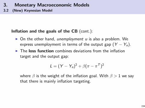
Inflation and the goals of the CB (cont.):
I On the other hand, unemployment u is also a problem. Weexpress unemployment in terms of the output gap (Y − Yn).
I The loss function combines deviations from the inflationtarget and the output gap:
L = (Y − Yn)2 + β(π − πT )2
where β is the weight of the inflation goal. With β > 1 we saythat there is mainly inflation targeting.
154

3. Monetary Macroeconomic Models3.2 (New) Keynesian Model
y
π
yn
πT
PCdecreasing utility
155

3. Monetary Macroeconomic Models3.2 (New) Keynesian Model
I Note that there might be problems of time-inconsistency(Barro-Gordon model, see next chapter).
I The consequences from this literature are that CB should becommitted to the inflation goal only.
I However, inflation is driven by the output gap, andmonetary policy operates with a lag = targets futureinflation arte. Therefore, for targeting inflation CB must havean eye also on the output gap (Svensson 1997).
I If the CB formulates an optimal policy path after a shock, weassume that CB is credible, so that for each t the inflationexpectations are following the announced path. Stochasticdeviations do not undermine credibility.
156

3. Monetary Macroeconomic Models3.2 (New) Keynesian Model
I Note that the PC is a constraint to the loss minimizationprogram!
I As long as PC with πE = πT is stable, the CB can determinefor any IS curve a real interest rate r such that themacroeconomic equilibrium can be achieved. It could respondto any demand shock in an optimal manner.
I If PC shifts, the long-run macroeconomic equilibrium cannotbe achieved but we can find the optimal compromise betweeninflation and output gap (which depends on parameter β).
157

3. Monetary Macroeconomic Models3.2 (New) Keynesian Model
y
π
yn
πT
PC
A
PC ′
B
B: stabilizing πTC
C: stabilizing ynD
D: best compromise
monetary policy rule
158

3. Monetary Macroeconomic Models3.2 (New) Keynesian Model
Analytically:
min L = (y − yn)2 + β(π − πT )2
s.t. π = πE + α(y − yn) (PC)
The PC can be directly plugged into the goal function.
Although the policy variable is r we can use y instead because with agiven IS curve, y could be directly achieved by the choice of r :
L = (y − yn)2 + β(πE + α(y − yn)− πT )2
∂L
∂y= 2(y − yn) + 2αβ(πE + α(y − yn)− πT )
FOC: 0 = (y − yn) + αβ(πE + α(y − yn)− πT )
Solving PC to πE = π − α(y − yn) and plugging into FOC:
0 = (y − yn) + αβ(π − πT )
(y − yn) = −αβ(π − πT )
which is the monetary policy response rule(downwards sloped in (π, y)-space). 159

3. Monetary Macroeconomic Models3.2 (New) Keynesian Model
Now we have the full 3-equation model:
y = A− ar (IS)
π = πE + α(y − yn) (PC)
(y − yn) = −αβ(π − πT ) (MR)
160

3. Monetary Macroeconomic Models3.2 (New) Keynesian Model
y
r
IS
re
ye
y
π
ye
PC
πT
MR
161

3. Monetary Macroeconomic Models3.2 (New) Keynesian Model
Variations:
I All variables could have a time index t.
I We can assume “adaptive” expectations πEt = πt−1.
I We can assume a dynamic IS curve: yt = A− art−1.
We will use these assumptions (dynamic 3-equation model).
Let’s do some exercises to find out how the model responds toshocks....
162

3. Monetary Macroeconomic Models3.2 (New) Keynesian Model
Inflation shock:
y
r
IS
re
ye
A
r0C
Dr1
y
π
ye
PC(πE = πT )
MR
πTA
PC(πE = π0)
π0B
y1
π1C
PC(πE = π1)
y2
π2 D
t
π
πT
shock
π0
t
y
ye
y1
t
r
re
r0
163

3. Monetary Macroeconomic Models3.2 (New) Keynesian Model
Inflation shock:
I We start in an equilibrium (point A).
I We have an inflation shock, shifting the this PC upwards andleading to π0 > πT (point B).
I CB responds according to the monetary policy rule by increasing thereal interest rate to r0 > re .
I This dampens inflation to π1 < π0 but leads also to an output gap:y1 < yn (point C)
I Inflation expectations are reduced to πE = π1, shifting the PCdownwards.
I Inflation rate falls, and CB responds by reducing r aas well (pointD).
I Process is going on until initial equilibrium is reached.
164

3. Monetary Macroeconomic Models3.2 (New) Keynesian Model
Temporary demand shock:
y
r
IS
re
ye
A
IS ′B
Cr0D
y
π
ye
PC(πE = πT )
MR
πTA
π0B
y0
PC(πE = π0)
π1C
y1
PC(πE = π1)
D
t
π
πT
shock
π0
t
y
ye
y0
y1
t
r
re
r0
165

3. Monetary Macroeconomic Models3.2 (New) Keynesian Model
Temporary demand shock:
I We start in an equilibrium (point A).
I IS curve shifts to the right for one period.
I With given r output and inflation increase to y0 > yn and π0 > πT .
I Expectations will adapt and thus PC shift upwards.
I CB intervenes according to the policy rule by increasing real interestrate to r0 > re .
I With the given new PC the realized point C implies now a negativeoutput gap y1 < yn, and a slightly reduced inflation rate π1.
I Expectations aeapt again, PC shifts downwards, inflation declines,CB reduces r , process converges to inirial situation again.
I As a result, we see an “overshooting” in the output.
I Note that all these adaption processes crucially dpend on theformation of expectations!
166

3. Monetary Macroeconomic Models3.2 (New) Keynesian Model
Permanent supply “shock”: (structural parameters z)
y
r
IS
reA
ye
r1C
y ′e
Dr ′e
y
π
ye
PC(πE = πT , ye)
MR
πTA
PC(πE = πT , y ′e)
MR ′
y ′e
π0 B
PC(πE = π0, y′e)
y1
π1C
D
t
π
πT
shock
π0
t
y
ye
y ′e
y1
t
r
rer ′er1
167

3. Monetary Macroeconomic Models3.2 (New) Keynesian Model
Permanent supply “shock”: (structural parameters z)
I Phillips Curve shifts downwards (same output yn at lower inflationrates, or at the same target inflation level highe equilibrium outputlevel y ′n).
I The optimal monetary response rule shifts as well because it isparametrized by the (new) equilibrium output level.
I Immeadiate drop of inflation to π0 (point B).
I Inflation expectations adapt to π0 so that Phillips curve shiftsfurther.
I Optimal policy response (reduction to r1, point C).
I Result is high output y1 at inflation rate π1.
I Now inflation expectations adapt to π1 (upwards shift of Phillipscurve) which also leads to policy responses.
I Phillips curve converges to the initial situation after the shock (withhigher equilibrium output).
168

3. Monetary Macroeconomic Models3.2 (New) Keynesian Model
(c) New Consensus Model: Small Open Economy
I GDP also consists of net exports, thus the IS curve reads
y = a(r0 − r) + cq (16)
with q = real exchange rate (in logs),and s is the spot rate (in logs).
I From definition of real exchange rate we have∆q = ∆s + πf − π.
I PPP: ∆s = π − πf .
I UIRP: ∆se = i − i f .
169

3. Monetary Macroeconomic Models3.2 (New) Keynesian Model
I Long run scenario: PPP holds true and no systematic error(∆se = ∆s). This implies:
i − i f = ∆se = ∆s = π − πf
end henceforthr = r f
I Consequence: if UIRP and PPP hold true, then r isexogenously determined by r f , thus there is no room formonetary policy in case of a small country, even in case offlexible exchange rates.
I CB can choose the nominal interest rate i which induceschanges of s and finally of inflation π.
I But this means that CB does not have any real effect.
170

3. Monetary Macroeconomic Models3.2 (New) Keynesian Model
I Short-run scenario: UIRP holds true, but not PPP
I Let q be the long-run equilibrium real exchange rate (in logs).For simplicity assume q = 0.
I For any deviation from q, the market participants excpect acorrection ∆q = α(q − q).
I Again, if UIRP holds true and there is no systematic error(∆se = ∆s) we have ∆q = r − r f .
I With q = 0 and assuming α = 1, it follows
r − r f = ∆q = α(q − q)
= −q⇒ q = r f − r
171

3. Monetary Macroeconomic Models3.2 (New) Keynesian Model
I Plugging into the IS curve:
y = a(r0 − r) + c(r f − r) = ar0 + cr f − (a + c)r
(IS curve is somehow flatter in (r , y)-space.)
I Therefore, the graphical analysis of the open economy case isessentially the same like for the closed economy case. Theimpact on the real sector is now enhanced via the interestrate effect on the exchange rate (UIRP).
172

4. Institutional Analysis of Monetary, Fiscal and Exchange Rate Policy
Outline:
4.1 Historical Exchange Rate Regimes
4.2 Rule Binding and Discretionary Policy in an Open Economy
4.3 Rules, Independence, Credibility – the Problem ofInterdependence of Monetary and Fiscal Policy
4.4 Governmental Debt, Inflation and Currency Crisis
173

4. Institutional Analysis of Monetary, Fiscal and Exchange Rate Policy
This chapter is about
I the interdependence of domestic and foreign monetary policy,
I the interdependence of fiscal policy with monetary policy –home and abroad,
I the role of rules
I the problems that occur if rules are not enforced
174
4. Institutional Analysis of Monetary, Fiscal and Exchange Rate Policy
4.1 Historical Exchange Rate Regimes
In principle, the IMF distinguishes the following exchange ratesystems:
I Dollarization, euroization
I Currency Board System
I Fixed parity (e.g. gold standard, gold exchange standard)
I Fixed parity within a band
I Crawling peg
I Crawling bend
I Managed floating
I Pure floating
These types cover all existing exchange rate regimes and currencyrelations.
175

4. Institutional Analysis of Monetary, Fiscal and Exchange Rate Policy
4.1 Historical Exchange Rate Regimes
Relevant Systems in the past:
I Gold Standard
I Gold Exchange Standard: the Bretton Woods System
I European Monetary System
I EMS 2
176

4. Institutional Analysis of Monetary, Fiscal and Exchange Rate Policy
4.1 Historical Exchange Rate Regimes
Following principles held in the gold standard:
I For each currency the price of gold was fixed
I Members had to sell and buy gold for the fixed price
I They also were obliged to maintain the relation of cash to gold
Bilateral exchange rates were the automatic result; an example:
I New York: 35 $ for an ounce gold
I London: 175 Shilling for an ounce gold
I The exchange rate was 5 Shilling for a $ or 4 $ for PoundSterling (£), as 20 shilling were 1 Pound. 4 $ for the £ wasthe mint parity. Governments were not obliged to acceptforeign currency.
177

4. Institutional Analysis of Monetary, Fiscal and Exchange Rate Policy
4.1 Historical Exchange Rate Regimes
If a central bank prints too much (too little) money, the currencydepreciates (appreciates) relatively to others. Arbitrage becomessensible; an example:
The monetary base in the US increases, gold price is unchanged.As a result, the parity is deviating from the mint parity andchanges into 4.5 $/£. An arbitrageur buys 1,000 ounces for 35,000$, trades the gold to London and sells it for 175,000 Shilling or8,375 £. He sells this sum for 4.5 $/£ into dollars and generatesprocced of 39,375 $. The profit is 4,375 $.
This mechanism left some leeway for the central bank, as thetransport of gold was not without costs for the arbitrageur.
178

4. Institutional Analysis of Monetary, Fiscal and Exchange Rate Policy
4.1 Historical Exchange Rate Regimes
The gold standard:
Dollar / Pound Sterling
volume of Sterling traded for Dollars
gold export point
gold import point
mint parity
179

4. Institutional Analysis of Monetary, Fiscal and Exchange Rate Policy
4.1 Historical Exchange Rate Regimes
Because of three important preconditions, the gold standard hadits problems:
I No lender of last resort
I The relative price between gold and the representative basketof commodities has to remain constant
I The amount of gold must increase with the growth rate.
The gold standard was in place from 1870 until 1913/14.
180

4. Institutional Analysis of Monetary, Fiscal and Exchange Rate Policy
4.1 Historical Exchange Rate Regimes
An example for the gold exchange standard is the BrettonWoods System (BWS). The US kept the price for gold constantat 35 $ per ounce and committed to sell gold for this price. Allother members kept their exchange rate to the Dollar within a1-per cent band constant.
Problem of the nth currency: since the US guaranteed the goldexchange, the other members had to maintain the exchange rate;obligations to intervene were exclusively theirs. This implies thatthe US is responsible for the inflation rates in whole system (aslong as there is no run on gold).
181

4. Institutional Analysis of Monetary, Fiscal and Exchange Rate Policy
4.1 Historical Exchange Rate Regimes
The system used a vast amount of capital controls andconvertibility restrictions.
The US used its degree of freedom to finance the Vietnam war viamoney press. Other countries had to buy dollars to maintain theexchange rate ⇒ imported inflation!
However: the undervalued currency of some countries (above allGermany) created an export-led growth.
182

4. Institutional Analysis of Monetary, Fiscal and Exchange Rate Policy
4.1 Historical Exchange Rate Regimes
The system got under stress from 1967 on: in November theBritish Pound was devalued; the Dollar was under pressure. In 1968the US weakened the obligation to sell gold.
The German Mark (as other currencies) were revalued in 1969; theGerman federal election campaign was strongly influenced by thedebate about the exchange rate.
In December 1971, the Smithsonian Agreement led to new paritiesand a wider band (5.5 per cent). 1972, the Pound left the BWS,and 1973 the German government introduced even stronger capitalcontrols. In March 1973, the system was abandoned.
183

4. Institutional Analysis of Monetary, Fiscal and Exchange Rate Policy
4.1 Historical Exchange Rate Regimes
The European Monetary System (EMS) was introduced in1979. Exchange rates were fixed (with the option of realignments),The European Currency Unit (ECU) was introduced; its value wascalculated according to a basket of commodities, which was basedon:
I Countries’ share in trade
I Countries’ share in GDP
I Countries’ quota in emergency cases
The band was ± 2.25 per cent; the obligation to intervene wassymmetrically distributed. A credit mechanism supported thesystem.
184

4. Institutional Analysis of Monetary, Fiscal and Exchange Rate Policy
4.1 Historical Exchange Rate Regimes
The system worked quite well until it was replaced by theEurosystem in 1999. Inflation was low on average, the GermanMark was dominating. Between 1987 and 1992 there were norealignments.
However, a crisis in 1992/1993 hit the system. The UK – that1990 had joined the system – was forced to leave it afterturbulences in September 1992 (with Italy). There were contagioneffects on France, Spain, Portugal, Ireland, Denmark and Belgium.1993, the bandwidth was increased to ± 15 per cent.
Italy later joined the system again.
185

4. Institutional Analysis of Monetary, Fiscal and Exchange Rate Policy
4.1 Historical Exchange Rate Regimes
What were the causes of the crisis?
I Different inflation rates
I Lack of credibility of monetary policy of some central banks
I Wrongly set exchange rates (British Pound)
I German re-unification
I Dismantling of capital controls
186

4. Institutional Analysis of Monetary, Fiscal and Exchange Rate Policy
4.1 Historical Exchange Rate Regimes
I With the foundation of the Eurosystem, the EuropeanMonetary System 2 (EMS2) was created. It contains thosecountries that did not qualify for the EMU in 1999.
I Exchange rates towards the Euro are fixed, again withbandwidth of ± 15 per cent. The Maastricht criteria hold formembers; once they meet them, the join the Eurozone.
I This time, the burden of intervention is with the members,since they want to become EMU members and have to keepthe exchange rate stable for two years.
187

4. Institutional Analysis of Monetary, Fiscal and Exchange Rate Policy
4.1 Historical Exchange Rate Regimes
I There is the chance to fix the exchange rate unilaterally andto bring about stability thereby. Ways are simple fixes,crawling pegs or currency boards.
I The latter will be presented and discussed in section 4.3.There have been several successful examples in recent history.
188

4. Institutional Analysis of Monetary, Fiscal and Exchange Rate Policy
4.1 Historical Exchange Rate Regimes
Conclusion:
I Fixed exchange rates allow the import of stability (EMS), butalso have the risk of spreading inflation (BWS); here theproblem of the nth currency was huge.
I A currency board can help with importing stability, if and onlyif it is backed by fiscal stability.
189

4. Institutional Analysis of Monetary, Fiscal and Exchange Rate Policy
4.2 Rule Binding and Discretionary Monetry Policy in an Open Economy
The core questions of this section are:I How to ensure low inflation?
I Remember: inflation is a monetary phenomenon ...I ... and it has its basis more often than not in fiscal problems
(section 4.4)
I How can the government solve the multi-stage PAP inmonetary policy?
I Defining principals and agents
I Should the government have discretionary leeways whenpursuing (monetary) policy or should it be restricted bygeneral rules?
I Who is responsible for monetary policy?
I Is deflation a real threat today?
190

4. Institutional Analysis of Monetary, Fiscal and Exchange Rate Policy
4.2 Rule Binding and Discretionary Monetry Policy in an Open Economy
What is the relevant PAP?
I Ownership and control are separated
I Who is the principal and who the agent in monetary policy?
I The PAP may occur prior to the contract (adverse selection)or afterwards (moral hazard)?
I What is the relevant problem in monetary policy?
I Solutions (Buba-Watcher)
191

4. Institutional Analysis of Monetary, Fiscal and Exchange Rate Policy
4.2 Rule Binding and Discretionary Monetry Policy in an Open Economy
“No form of organization, of course, can obtain wisepolicy from men who have no wisdom in them. But poororganization can obtain unwise policy from men whohave wisdom in them.” (Hart 1948, p. 515).
⇒ Popper
⇒ This can be called “The Alamo-effect”
192

4. Institutional Analysis of Monetary, Fiscal and Exchange Rate Policy
4.2 Rule Binding and Discretionary Monetry Policy in an Open Economy
The PAP in monetary policy:
1. Principal: public
1. Agent: government = 2. Principal
non-observable behaviordelegation of responsibility(assignment)
2. Agent: central bank
non-observable behaviormonetary policywith different goals
3. Principal: future employer
specific concernsinofficial relation
good conduct
193

4. Institutional Analysis of Monetary, Fiscal and Exchange Rate Policy
4.2 Rule Binding and Discretionary Monetry Policy in an Open Economy
Solutions to the PAP:
I k-rule
I Legal status for k-rule
I Selection “good” policymakers, i.e. Rogoff’s conservativecentral banker
I Contracts with central bankersI Monetary policy rules:
I Independent central bankI Currency boardI Denationalization (currency competition or dollarization)
194

4. Institutional Analysis of Monetary, Fiscal and Exchange Rate Policy
4.2 Rule Binding and Discretionary Monetry Policy in an Open Economy
Aspects of rule binding in monetary policy:
I Target (inflation rate, money base, interest rate)
I Legal status
I Degree of flexibility
I Simplicity, transparency, stability over time
195

4. Institutional Analysis of Monetary, Fiscal and Exchange Rate Policy
4.2 Rule Binding and Discretionary Monetry Policy in an Open Economy
Nobel prize 2004 to F.E. Kydland and E.C. Prescott
“for their contributions to dynamic macroeconomics: thetime consistency of economic policy and the drivingforces behind business cycles.”
I Kydland, F.E., Prescott, E.C. (1977), Rules Rather thanDiscretion: The Inconsistency of Optimal Plans. Journal ofPolitical Economy 85, 473-493.
I Belke, A., Selzer, R. (2005), Nobelpreis furWirtschaftswissenschaften 2004 an Finn E. Kydland undEdward C. Prescott. WiSt 2, S.99-104.
196

4. Institutional Analysis of Monetary, Fiscal and Exchange Rate Policy
4.2 Rule Binding and Discretionary Monetry Policy in an Open Economy
Time consistency:
I Policymakers announces optimal policy
I Agents form expectations
I Agents make decisions and agree on contracts
I Because of these expectations and contracts it is no longeroptimal for the policymaker to follow the announced plan; shechanges the plan and surprises the agents
⇒ If agents are rational, they will not believe policyannouncements in the future.
197

4. Institutional Analysis of Monetary, Fiscal and Exchange Rate Policy
4.2 Rule Binding and Discretionary Monetry Policy in an Open Economy
Rational expectations:
I On average correct
I Imply an equilibrium
I Policymakers have to consider reactions of agents on policyannouncements (Lucas critique)
I Rational individuals cannot be cheated systematically
198

4. Institutional Analysis of Monetary, Fiscal and Exchange Rate Policy
4.2 Rule Binding and Discretionary Monetry Policy in an Open Economy
The Barro-Gordon Model
Literature:
I Barro, R.J., Gordon, D.B. (1983), A Positive Theory ofMonetary Policy in a Natural Rate Model. Journal of PoliticalEconomy 91, pp. 589
I Barro, R.J., Gordon, D.B. (1983), Rules, Discretion, andReputation in a Model of Monetary Policy. Journal ofMonetary Economics 12, 101-122.
199

4. Institutional Analysis of Monetary, Fiscal and Exchange Rate Policy
4.2 Rule Binding and Discretionary Monetry Policy in an Open Economy
I Phillips-Curve:u = un − (π − πe)
I Objective function is a loss function:
W = −π2 − λu2
= −π2 − λ(un − π + πe)2
I Maximizing the objective function
dW
dπ= −2π + 2λ(un − π + πe) = 0, (FOC)
⇒ π∗ =λ
1 + λ(un + πe) = Φ(πe).
This is the central bank’s best response function.
200

4. Institutional Analysis of Monetary, Fiscal and Exchange Rate Policy
4.2 Rule Binding and Discretionary Monetry Policy in an Open Economy
π
uun
long-term PC
short-term PCswith different πe
indifferencecurves W
For each πe (and thus given short-run PC), central bank chooses optimal π.
π
πe
Φ(πe)
best response function
201

4. Institutional Analysis of Monetary, Fiscal and Exchange Rate Policy
4.2 Rule Binding and Discretionary Monetry Policy in an Open Economy
Time inconsistent policy:
I Announcement: π = 0.
I If expectations are naıve, then πe = 0.
I Inserting πe = 0 into the reaction function yields“surprise inflation”
πsur = Φ(πe) =λ
1 + λ(un + πe)
=λ
1 + λun
I Welfare is
Wsur = − λ
1 + λu2
n
202

4. Institutional Analysis of Monetary, Fiscal and Exchange Rate Policy
4.2 Rule Binding and Discretionary Monetry Policy in an Open Economy
π
uun
long-term PC
short-term PCwith πe = 0
Wsur
A
π
πe
Φ(πe)
πsur
203

4. Institutional Analysis of Monetary, Fiscal and Exchange Rate Policy
4.2 Rule Binding and Discretionary Monetry Policy in an Open Economy
Consequences:
I Inflation expectations are systematically wrong in case of“surprise inflation”.
I Decisions of private agents depend on expectations. Thus,bigger expectation errors cause less decision quality. Ifexpectations are not systematically (systematically not?)wrong, decisions are optimal ⇒ rational expectations
I Then, the objective function is:
Z = −(π − πe)2
I Maximizing it, yields:πe = π
204

4. Institutional Analysis of Monetary, Fiscal and Exchange Rate Policy
4.2 Rule Binding and Discretionary Monetry Policy in an Open Economy
I Thus, the central bank assumes rational expectations.
I Equalizing πe = π and solving the reaction function Φ(πe) toπ yields:
π = Φ(πe) =λ
1 + λ(un + π)
⇒ πrat = λun > 0
I The only credible policy is positive inflation (inflation bias)πrat > 0.
I Welfare thus is:
Wrat = −(1 + λ)λu2n < Wsur = − λ
1 + λu2
n
205

4. Institutional Analysis of Monetary, Fiscal and Exchange Rate Policy
4.2 Rule Binding and Discretionary Monetry Policy in an Open Economy
π
uun
long-term PC
PC (πe = 0)
Wsur
A
PC (πe = πrat )
Wrat
B
πrat
π
πe
Φ(πe)
πsur
45
π = πe
πrat
206

4. Institutional Analysis of Monetary, Fiscal and Exchange Rate Policy
4.2 Rule Binding and Discretionary Monetry Policy in an Open Economy
I Alternative: binding rule π = 0⇒ no discretionary leeway, pre-commitment.
I Inflation expectation πe = 0 is then rational.
I Welfare in this case is:
Wrule = −λu2n
I It holds thatWsur >Wrule >Wrat
207

4. Institutional Analysis of Monetary, Fiscal and Exchange Rate Policy
4.2 Rule Binding and Discretionary Monetry Policy in an Open Economy
π
u
long-term PC
PC (πe = 0)
PC (πe = πrat )
Wsur Wrat
B
A
Wrule
Cπrat
π
πe
Φ(πe)
45
π = πe
πsur
πrat
208

4. Institutional Analysis of Monetary, Fiscal and Exchange Rate Policy
4.2 Rule Binding and Discretionary Monetry Policy in an Open Economy
Summary:
I Efficiency of monetary policy depends on institutional setting(rules vs. discretion)
I Strict rule binding is more efficient.
Problems:
I Inflation perfectly manageable?
I Static model
I Full information
I No stochastic influences
I How realistic is the assumption of rational expectations?
209

4. Institutional Analysis of Monetary, Fiscal and Exchange Rate Policy
4.2 Rule Binding and Discretionary Monetry Policy in an Open Economy
Variation: repeated interaction
I Modeled as a infinite strategic game between central bankand public.
I Discounted welfare is:
V =∞∑
t=0
1
(1 + r)tWt =
∞∑t=0
δtWt
I Central bank tries to build up reputation: announcing π = 0and delivering.
I Expectations πe = 0 are fulfilled.
I Higher welfare than in static model possible.
210

4. Institutional Analysis of Monetary, Fiscal and Exchange Rate Policy
4.2 Rule Binding and Discretionary Monetry Policy in an Open Economy
I Expectations are interpreted as strategic variable.
I Mechanism to form expectations:
πet =
πrule = 0 if πk = 0 ∀k < t
πrat = λun else
⇒”Trigger mechanism“.
I Public believes central bank’s zero inflation announcementonly until the central bank deviates for the first time
I Thereafter, the public always believes the rational policysolution: πrat > 0, which will be realised.
211

4. Institutional Analysis of Monetary, Fiscal and Exchange Rate Policy
4.2 Rule Binding and Discretionary Monetry Policy in an Open Economy
I On the one hand, the central bank faces the incentive toincrease welfare by means of a “surprise inflation”:Wsur >Wrule .
I On the other hand, there is a deterrence effect, since thecentral bank then faces πe = πrat , which leads to futurewelfare losses Wrat <Wrule .
I It depends on the discount factor!
212

4. Institutional Analysis of Monetary, Fiscal and Exchange Rate Policy
4.2 Rule Binding and Discretionary Monetry Policy in an Open Economy
The central bank compares the discounted welfare when sticking tothe announcement:
Vrule =∞∑
t=0
δtWrule =∞∑
t=0
δt [−λu2n] = − 1
1− δλu2
n
with the discounted welfare after one deviation from theannouncement:
Vsur = Wsur +∞∑
t=1
δtWrat
= − λu2n
(1 + λ)+∞∑
t=1
δt [−(1 + λ)λu2n]
= − λu2n
(1 + λ)− δ
(1− δ)(1 + λ)λu2
n
213

4. Institutional Analysis of Monetary, Fiscal and Exchange Rate Policy
4.2 Rule Binding and Discretionary Monetry Policy in an Open Economy
I It sticks to the rule, if
Vrule > Vsur
− 1
(1− δ)[λu2
n] > − λu2n
(1 + λ)+
δ
(1− δ)[−(1 + λ)λu2
n]
⇒ δ ≥ 1
2 + λ= δ∗
⇐⇒ 1
1 + r≥ 1
2 + λ⇐⇒ r∗ ≤ 1 + λ
I The more employment is important for the central bank (λlarge), the higher is the threshold for the discount rate inorder to let the central bank stick to the rule.
214

4. Institutional Analysis of Monetary, Fiscal and Exchange Rate Policy
4.2 Rule Binding and Discretionary Monetry Policy in an Open Economy
Conclusion:
Even without a formal rule, zero inflation is possible if the centralbank’s discount rate r is low enough (δ ≥ δ∗, r ≤ r∗). Themechanism is to build up reputation.
215

4. Institutional Analysis of Monetary, Fiscal and Exchange Rate Policy
4.2 Rule Binding and Discretionary Monetry Policy in an Open Economy
Problems:
I Infinite number of equilibria, lot of which imply positiveinflation rates, depending on trigger mechanism.
I Trigger mechanism difficult to measure empirically.
I Strategic expectation formation doubtful: fallacy ofcomposition.
I Full information.
216

4. Institutional Analysis of Monetary, Fiscal and Exchange Rate Policy
4.2 Rule Binding and Discretionary Monetry Policy in an Open Economy
Further extensions:
I Incomplete information
I Stochastic shocks
217

4. Institutional Analysis of Monetary, Fiscal and Exchange Rate Policy
4.2 Rule Binding and Discretionary Monetry Policy in an Open Economy
Incomplete information:
Literature:
I Backus, D., Driffill, J. (1985), Inflation and Reputation.American Economic Review 75, 530-538.
I Cukierman, A. (2000), Establishing a Reputation forDependability by Means of Inflation Targets. Economics ofGovernance 1, 53-76.
218

4. Institutional Analysis of Monetary, Fiscal and Exchange Rate Policy
4.2 Rule Binding and Discretionary Monetry Policy in an Open Economy
I Basic characteristics of the Backus-Driffill model:
I Central bank’s objective function not known to the publicI Dynamic game (two rounds) with the formation of reputation
I Loss function: W = −π2 − λuI Monetary policy in the first stage leads the public to build
expectations about the type of central banker(“falcon”, i.e. λ = 0, vs. “dove”, i.e. λ > 0).
I The probability p and 1− p respectively of central bankers tobe of either type is known.
I Central banker may use this setting to form expectations andminimize the loss function.
219

4. Institutional Analysis of Monetary, Fiscal and Exchange Rate Policy
4.2 Rule Binding and Discretionary Monetry Policy in an Open Economy
I Case 1: Type falcon: Maximizing W yields
π1 = 0, π2 = 0
I Case 2: Type dove: Maximizing W yields
∂W
∂π= −2π + λ = 0 (FOC)
⇒ π∗ =1
2λ
220

4. Institutional Analysis of Monetary, Fiscal and Exchange Rate Policy
4.2 Rule Binding and Discretionary Monetry Policy in an Open Economy
I If inflation is positive in stage 1 (π1 = π∗ > 0), the public canbe sure of the central banker’s type; she is a dove. In stage 2the public will then expect πe
2 = π2 = π∗ > 0.
I However, a dove may have the incentive to mimic a falcon tobring down inflationary expectations for stage 2 (surpriseinflation). So, π1 = 0 does not clarify the type.
I Question: when does it pay off for a dove to hide her type andmimic a falcon?
221

4. Institutional Analysis of Monetary, Fiscal and Exchange Rate Policy
4.2 Rule Binding and Discretionary Monetry Policy in an Open Economy
I For low time preference (high δ) and small prior probability ofa dove (p) a pooling equilibrium occurs (i.e. both typeschoose zero inflation in stage 1).
I For high time preference a separating equilibrium is likely(each type chooses his preferred inflation rate).
I However, there are cases, which are less clear, ifδ ∈ ( 1
2 ,12
1(1−p) )
222

4. Institutional Analysis of Monetary, Fiscal and Exchange Rate Policy
4.2 Rule Binding and Discretionary Monetry Policy in an Open Economy
Basic characteristics of the Cukierman model:
I Two types of government with identical objective function,but different abilities to commit; type D is able to commitcredibly, type W is not.
I Objective function is directed at employment and pricestability
I Dynamic game (two rounds) with the formation of reputation
I Central bank can influence but not set inflation rates:
πreali = πi + εi , ε ∼ U[−ai ,+ai ]
with 0 < aD < aW , implying that the dependable central bankis better equipped to meet its objective than the weak centralbank.
223

4. Institutional Analysis of Monetary, Fiscal and Exchange Rate Policy
4.2 Rule Binding and Discretionary Monetry Policy in an Open Economy
Results (intuitive):
I Inflation of period 1 determines the expectations andreputation in period 2.
I A dependable central bank (type D) has an interest to createa separating equilibrium, whereas a weak central bank (typeW) rather prefers a pooling equilibrium to gain from thereputation effect.
I The more conservative D, the more pressure on W to strivefor low inflation.
224

4. Institutional Analysis of Monetary, Fiscal and Exchange Rate Policy
4.2 Rule Binding and Discretionary Monetry Policy in an Open Economy
I The model emphasizes the ability of central bank to createprice stability.
I This holds even under the assumption that employment is anobjective for the central bank.
I The chance to bind to rules disciplines a central bank.
I Stochastic elements are realistic.
225
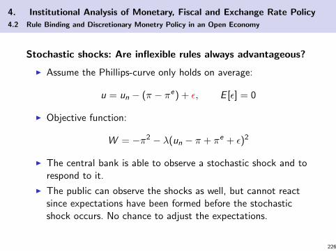
4. Institutional Analysis of Monetary, Fiscal and Exchange Rate Policy
4.2 Rule Binding and Discretionary Monetry Policy in an Open Economy
Stochastic shocks: Are inflexible rules always advantageous?
I Assume the Phillips-curve only holds on average:
u = un − (π − πe) + ε, E [ε] = 0
I Objective function:
W = −π2 − λ(un − π + πe + ε)2
I The central bank is able to observe a stochastic shock and torespond to it.
I The public can observe the shocks as well, but cannot reactsince expectations have been formed before the stochasticshock occurs. No chance to adjust the expectations.
226

4. Institutional Analysis of Monetary, Fiscal and Exchange Rate Policy
4.2 Rule Binding and Discretionary Monetry Policy in an Open Economy
Results: (intuitive)
I Welfare under a flexible rule (taking the shocks into account)may be higher than both welfare under a fixed rule and underdiscretion
I Rationale: the central bank can react to shocks in order toincrease employment without creating higher inflationexpectations.
I Important lesson for policymakers: in the presence ofstochastic shocks, they have more flexibility without hurtingzero-inflation expectations.
Problems:
I Such a rule cannot be formulated in a general form
I Distinction between a shock and a preference of the centralbank for the employment goal difficult ⇒ loss of reputation
227

4. Institutional Analysis of Monetary, Fiscal and Exchange Rate Policy
4.3 Rules, Independence, Credibility – Interdependence of Monetary and Fiscal Policy
I The lesson of the theoretical models is that we need a crediblepolicy announcement to secure price stability.
I According to the theoretical literature, the problem is apositive λ, i.e. the focus of the central bank on employment.Thus, one has to secure that λ = 0 holds for the central bank.
I Therefore, it is not sufficient to formulate a binding rule; ithas to be enforceable. Indeed, empirical evidence shows thatstrict rules are no sufficient to guarantee price stability. Whatconstitutes the credibility of a rule?
228

4. Institutional Analysis of Monetary, Fiscal and Exchange Rate Policy
4.3 Rules, Independence, Credibility – Interdependence of Monetary and Fiscal Policy
Distinction ex-post vs. ex-ante credibility is necessary.
I Ex post: interest rate spreads, capital flows, inflation etc.
I Ex ante: compatibility of monetary commitment witheconomic order and other elements of policy:
I Judiciary independenceI Economic freedomI Public attitude to inflationI Fiscal stabilityI Labor market flexibility
229

4. Institutional Analysis of Monetary, Fiscal and Exchange Rate Policy
4.3 Rules, Independence, Credibility – Interdependence of Monetary and Fiscal Policy
Distinction between credibility and reputation
I Credibility: policy announcement
I Reputation: policymaker
230

4. Institutional Analysis of Monetary, Fiscal and Exchange Rate Policy
4.3 Rules, Independence, Credibility – Interdependence of Monetary and Fiscal Policy
Commitment mechanisms:
I It is important that the government commits to stability,otherwise the PAP is not solved
I Constitutional decision
I Legitimation
I Participation
231

4. Institutional Analysis of Monetary, Fiscal and Exchange Rate Policy
4.3 Rules, Independence, Credibility – Interdependence of Monetary and Fiscal Policy
Central bank independence (CBI):
I De jure vs. de facto
I Goal vs. instrument independence
I What drives CBI?
I Clearly defined goalsI Clear rules about loans to the governmentI Rules about decision making processes within the bankI Rules about appointment and dismissal of the directorateI Rules about the government’s relation to the bankI Rules about external relations
I How to measure CBI?
232

4. Institutional Analysis of Monetary, Fiscal and Exchange Rate Policy
4.3 Rules, Independence, Credibility – Interdependence of Monetary and Fiscal Policy
Source: (Maliszewski 2000) Cukierman Freytag (2001)GMT (CBI) et al. (2002) (CBI) (monetary
commitment)Method: adding up (0-16) average (0-1) average (0-1)Groups:CEO - term length - term lengths - expertise
- who appoints CEO? - who appoints? - dismissal- dismissal - dismissal- who appoints board members? - other offices- governmental board member?
31.25 per cent 20 per cent 10 per centpolicy - governmental approval - who formulates? - final authorityformu- - responsibility for policy - final authority - accountabilitylation - dispute settlement - CB budget - bank regulation
- discount rate- accountability- bank regulation
37.5 per cent 15 per cent 20 per cent
233

4. Institutional Analysis of Monetary, Fiscal and Exchange Rate Policy
4.3 Rules, Independence, Credibility – Interdependence of Monetary and Fiscal Policy
Source: (Maliszewski 2000) Cukierman Freytag (2001) (mone-GMT (CBI) et al. (2002) (CBI) tary commitment)
Method: adding up (0-16) average (0-1) average (0-1)Groups:policy n.a. - objective - objectiveobjective - constitutional level
15 per cent 20 per centlending - direct credit facility - advances - direct loansrestrictions (4 components) - securitised lending - primary market
- primary market - who decides?- circle of borrowers- types of limit- maturity of loans- interest rates- primary market
31.25 per cent 50 per cent 20 per cent
234

4. Institutional Analysis of Monetary, Fiscal and Exchange Rate Policy
4.3 Rules, Independence, Credibility – Interdependence of Monetary and Fiscal Policy
Source: (Maliszewski 2000) Cukierman Freytag (2001) (mone-GMT (CBI) et al. (2002) (CBI) tary commitment)
Method: adding up (0-16) average (0-1) average (0-1)Groups:external n.a. n.a. - ER regimeaspects - convertibility
- multiple ER?- currency competition
30 per cent
The percentages show the weights given to the group.Source: Freytag (2007).
235

4. Institutional Analysis of Monetary, Fiscal and Exchange Rate Policy
4.3 Rules, Independence, Credibility – Interdependence of Monetary and Fiscal Policy
I The theoretical analysis suggests a strong empirical causalrelation between commitment and inflation. This is difficult toobtain.
I For developing countries, it does not show. For industrializedcountries, we can see the relation.
I It becomes clearer, if we incorporate institutional constraints(compatibility).
236

4. Institutional Analysis of Monetary, Fiscal and Exchange Rate Policy
4.3 Rules, Independence, Credibility – Interdependence of Monetary and Fiscal Policy
237

4. Institutional Analysis of Monetary, Fiscal and Exchange Rate Policy
4.3 Rules, Independence, Credibility – Interdependence of Monetary and Fiscal Policy
Is CBI still important?
I Demands for accomodation
I Assignment
I Balance sheet operations, QE#1 and QE#2
I Is the multiplier still working?
I Inflation or deflation?
I Enforcement
See later section 4.4 for a discussion of rules.
238

4. Institutional Analysis of Monetary, Fiscal and Exchange Rate Policy
4.3 Rules, Independence, Credibility – Interdependence of Monetary and Fiscal Policy
Currency Board is an alternative to central banking. A currencyboard system (CBS) has the following properties:
I Complete backing of the monetary base with forex or gold
I Money issue only against forex
I Full convertibility
I Lack of monetary autonomy
I Dependence of international flows for money issue
239
4. Institutional Analysis of Monetary, Fiscal and Exchange Rate Policy
4.3 Rules, Independence, Credibility – Interdependence of Monetary and Fiscal Policy
Is a CBS a guarantee for price stability?Is the PAP solved automatically? NO!
I Institutional backing is still necessary
I Choice of exchange currency is important
I Currency must not be overvalued in real term
I No lender of last resort ⇒ can be an advantage or adisadvantage!
240

4. Institutional Analysis of Monetary, Fiscal and Exchange Rate Policy
4.3 Rules, Independence, Credibility – Interdependence of Monetary and Fiscal Policy
Examples for successful currency boards comprise:
I West African Currency Board (1913)
I Hong Kong (1983)
I Argentina (1991)??
I Estonia (1992)
I Lithuania (1994)
I Bulgaria (1997)
241

4. Institutional Analysis of Monetary, Fiscal and Exchange Rate Policy
4.3 Rules, Independence, Credibility – Interdependence of Monetary and Fiscal Policy
Recent example for discussions: ZimbabweI Inflation rate in early 2009: 200,000,000 per cent; the system
of relative price did not workI Suggestions:
I CBS (Steven Hanke 2008)I Randization (SA interim President Motlanthe 2009)I Fixing the Zim-$ to the Rand (Draper and Freytag 2009)
I Currently dollarization takes place in a multi currency system
Kramarenko,V., L. Engstrom, G. Verdier, G. Fernandez, S.E. Oppers, R.
Hughes, J. McHugh, and W. Coats (2010), Zimbabwe: Challenges and
Policy Options after Hyperinflation, Washington. D.C., IMF.
I New inflationary threats in 2016; government restrictscirculation of Dollars and plans the emission of new notes
(http://www.economist.com/news/middle-east-and-africa/
21698658-lock-up-your-dollars-right-now-mugabenomics-
back-who-wants-be)242

4. Institutional Analysis of Monetary, Fiscal and Exchange Rate Policy
4.3 Rules, Independence, Credibility – Interdependence of Monetary and Fiscal Policy
Empirical Evidence: on average, a CBS is superior to a centralbank regime. However:
“A currency board works well when a currency boardworks well!” (G.Calvo)
In other words: there are preconditions, which have to be met tomake a CBS work. In the cases, a CBS was introduced, theseconditions were regularly met (the exception being Argentina).
243

4. Institutional Analysis of Monetary, Fiscal and Exchange Rate Policy
4.4 Governmental Debt, Inflation and Currency Crisis
I As said before, there is evidence that hyperinflation is alwayscaused by fiscal problems (Fischer, Sahay and Vegh 2002).Therefore, it makes sense to take a look at fiscal problems, i.e.governmental debt.
I Public debt per GDP is much higher in OECD countries thanin developing countries.
244

4. Institutional Analysis of Monetary, Fiscal and Exchange Rate Policy
4.4 Governmental Debt, Inflation and Currency Crisis
General government consolidated gross debt as a percentage of GDP
EU (27) Euro area (19) Greece Germany1999 65.7 71.6∗ 94.0 60.92000 61.9 69.1∗ 103.4 59.72001 61.0 68.1∗ 103.7 58.82002 60.4 67.9∗ 101.7 60.42003 61.8 69.0∗ 97.4 63.92004 61.3 68.4 102.9 64.72005 61.9 69.2 107.4 66.92006 60.5 67.3 103.6 66.32007 57.9 64.9 103.1 63.52008 61.0 68.5 109.4 64.92009 73.1 78.3 126.7 72.42010 78.5 83.8 146.2 81.02011 81.1 86.0 172.1 78.32012 83.8 89.3 159.6 79.62013 85.5 91.1 177.7 77.22014 86.8 92.0 180.1 74.72015 85.2 90.7 176.9 71.22016 85 90 178 68.52017 81.6 86.7 178.6 64.1∗ EMU 17; Source: EuroStat
245

4. Institutional Analysis of Monetary, Fiscal and Exchange Rate Policy
4.4 Governmental Debt, Inflation and Currency Crisis
Is public debt a general problem? No!
When does it become a problem?
I Public investment is not increasing with debtI Government’s discount rate higher than real interest rate?
I a problem of democraciesI regardless of the state of development
I Public is myopic (rational expectations??)
I Ricardian equivalence?
246

4. Institutional Analysis of Monetary, Fiscal and Exchange Rate Policy
4.4 Governmental Debt, Inflation and Currency Crisis
I European debt crisis:
I Public mismanagement (Greece since ...)I Original sin (Germany/France 2003)I Troubled banks due to real estate defaults and global financial
crisis (Spain, Ireland)I Refusal to rescue banks a second time after 2008 in France
and Germany ⇒ bail out, breaching Art. 125I Structural adjustment program insufficient, downgrading of
Greece et al. (GIPS), increasing spreadI ECB bought Greek public bondI TARGET2 / ESM / QEI What role for speculators?I Who are the main speculators or gamblers?
247

4. Institutional Analysis of Monetary, Fiscal and Exchange Rate Policy
4.4 Governmental Debt, Inflation and Currency Crisis
I The main threat so far is the institutional laxity!
I Inflation is only a threat if the ECB permanently increases themonetary base and if the financial sector raises M3 (slide 22).
I Nevertheless, it cannot be excluded that the ECB has to writeoff public bonds, it has purchased (against its statute). In thiscase, the ECB faces capital losses, which have to be borne bythe tax payers.
I Or the monetary base increases ⇒ inflationary pressure.
I Thus, the European public debt crisis eventually threatens toend up in a currency crisis.
248

4. Institutional Analysis of Monetary, Fiscal and Exchange Rate Policy
4.4 Governmental Debt, Inflation and Currency Crisis
Is deflation a real threat?
I Inflation rate very low in Euroland.
I Deflation may cause the crisi to deepen, if the price level fallsover a longer time, which reduces the public’s trust andwillingness to trade, since it expects stronger price cuts in thefuture. This might lead to a depression.
I However, how can GIPS-countries gain in pricecompetitiveness, if devaluation is no choice?
I This imposes pressure on the ECB. How independent is theECB?
249

4. Institutional Analysis of Monetary, Fiscal and Exchange Rate Policy
4.4 Governmental Debt, Inflation and Currency Crisis
Is inflation a monetary phenomenon?
or
Is money and inflationary phenomen?
How to interpret the Quantity Equation M · v = P · Y ?
250

4. Institutional Analysis of Monetary, Fiscal and Exchange Rate Policy
4.4 Governmental Debt, Inflation and Currency Crisis
M · v = P · Y
Phillips Curve
credit Dcredit S
i
reserve Dreserve S
M0 ipolicy
r
ISC
urv
e
M0 ·m = Mresiduals
The velocity of money as well as the money multiplier emerge as
endogenously determined residulas from macroeconomic relationships.
Both equations are seen as simply algebraic relationships.
251

4. Institutional Analysis of Monetary, Fiscal and Exchange Rate Policy
4.4 Governmental Debt, Inflation and Currency Crisis
Consider a Cash-in-advance argument for money demand, and a dynamicNKM model with a forward looking monetary policy rule:
yt = Eyt+1 − αrt (IS)
πt = Eπt+1 + γ2yt (PC)
rt = δ1Eπt+1 + δ2Eyt+1 + µt (MPR)
mt − pt = yt + y∗t (CIA)
This leads to
mt − pt = Eyt+1 + y∗t︸ ︷︷ ︸exp. output
−αrt (M)
or in growth rates
mgt − πt = (Eyt+1 − Eyt) + (y∗t − y∗t−1)− α(rt − rt−1) (Q)
= (1− αδ2)(Eyt+1 − Eyt)− αδ1(Eπt+1 − Eπt)
− α(µt − µt−1) + (y∗t − y∗t−1)
Observe that (M) is the Quantity Equation, and (Q) the QuantityEquation in growth rates. Velocity is tied to real interest rate.
252

4. Institutional Analysis of Monetary, Fiscal and Exchange Rate Policy
4.4 Governmental Debt, Inflation and Currency Crisis
−2 0 2 4
−1
−0.5
0
0.5
real interest
velo
city
−2 0 2 4
−1.4
−1.2
−1
−0.8
real interest
velo
city
−2 0 2 4
0.5
1
1.5
real interest
velo
city
−2 0 2 40.2
0.3
0.4
0.5
real interest
velo
city
Real interest rate versus velocity of money (left panel: M1, right panel: M3, upper row: velocity as
ln(Y nom)− ln(M), lower row: velocity as Y nom/M, red filled: pre 12/2008, not filled: post 12/2008, blue X:
German 10-year gov. bonds rate) 253

5. Currency Crisis
Outline:
5.1 Models of Currency CrisisI IntroductionI First Generation ModelI Second Generation ModelsI Third Generation Models
5.2 Currency Crisis in a Monetary Union
Literature:
I Breuer, J.B. (2004), An Exegesis on Currency and Banking Crises.Journal of Economic Surveys Vol. 18 (3), pp. 293-320.
I Agenor, P.-R., Flood, R.P. (1994), Macroeconomic Policy, SpeculativeAttacks, and Balance of Payments Crises, in: F. van der Ploeg (ed.), TheHandbook of International Macroeconomics (ch. 8), Cambridge Mass.:Blackwell.
I Garber, P.M., Svensson, L.E.O. (1995), The Operation and Collapse ofFixed Exchange Rate Regimes, in: G.M. Grossman, K. Rogoff (eds.),Handbook of International Economics Vol. III (ch. 36), Amsterdam et al.:Elsevier.
254

5. Currency Crisis5.1 Models of Currency Crisis
Currency Crisis:
I Strong, fast, and permanent devaluation of a currency.
I Typically, a crisis means that a fixed exchange rate regimebreaks down by a speculative attack. In a crisis, the centralbank will lose most of their reserves.
I Negative macroeconomic shocks as a consequence (however,in many cases negative macroeconomic developments are thesource of a CC which reveals this development)
Reasons for a CC change in time (first, second, third generationmodels)
Are CC “bad”? Should policy try to avoid them?
255

5. Currency Crisis5.1 Models of Currency Crisis
I A currency crisis can be related to a (public) debt drisis:I Public debt crisis as a cause for currency crisis: Monetary
expansion, increasing risk of insolvency reduces trust intostability of the currency.
I Currency crisis can induce debt crisis if the government hasprimarly external debt which is then upvalued.
I A currency crisis can be related to bank crisis.
256

5. Currency Crisis5.1 Models of Currency Crisis
Identifying a Currency Crisis:
Eichengreen, B., Rose, A., Wyplosz, C. (1994), Speculative attacks onpegged exchange rates: an empirical exploration with special reference tothe European monetary system. NBER Working Paper No. 4898.
Reinhart, C., Kaminsky, G. (1999), The Twin Crises: the causes of
banking and balance-of-payment problems. American Economic Review
89(3), 473-500.
I Strong devaluation pressure on the exchange rate.
I Loss of reserves because central bank tries to stabilizeexchange rate.
I Increase of interest rates.
257

5. Currency Crisis5.1 Models of Currency Crisis
Market Turbulence Index:
MTI =e
σe− R
σR+
i
σi
I This is a combination of the growth rates (positive ornegative) of the exchange rate, the reserves, and the interestrates, weighetd with their volatility (to avoid that a variablewith a strong volatility dominates the result).
I When the MTI increases by a certain k-multiple of itsstandard deviation for n months (e.g.: 2), then we identify acrisis where the strength of the crisis is classified by k .
258

5. Currency Crisis5.1 Models of Currency Crisis
ER regime period number of number ofcurrency crisis bank crisis
gold standard 1880-1913 22 (0.65) 30 (0.88)ca. WW I 1913-1919 0 (0) 0 (0)between WW 1919-1939 48 (2.3) 47 (2.2)ca. Bretton Woods 1940-1971 45 (1.4) 1 (0.03)Post Bretton Woods 1972-1998 162 (6) 60 (2.2)
1998-2002 7 (1.4) 3 (0.6)values in brackets: p.a.
Surce: Breuer (2004), S.297
259

5. Currency Crisis5.1 Models of Currency Crisis
First Generation Models
I Starting with a fixed exchange rate regime
I Exogenously given behavior of the government
I Free capital movement
I Macroeconomic data become worse: increasing governmentaldebt, excessive monetary expansion. Peg does not reflect themacroeconomic situation anymore. Pressure on central bankto defend the peg.
I Speculation against the currency
Examples: Chile 1971-74, Bolivia 1982-85, Uruguay 1982, Peru1987, Brazil 1989-90, Brazil 1999, Argentina 2001
260

5. Currency Crisis5.1 Models of Currency Crisis
Speculation against the currency:
I Fixed exchange rate parity and “fundamental” exchange rate(e.g. given by IRP, PPP, and other macroeconomicconsiderations) are more and more diverging.
I Agents expect a depreciation = adjustment to thefundamental rate (realignment or switch to flexible exchangerates).
I Excess demand for strong foreign currency, excess supply ofweak domestic currency.
I Central bank has to intervene and to sell reserves of foreigncurrency. This can be done only if there are still significantreserves.
261

5. Currency Crisis5.1 Models of Currency Crisis
I If reserves are completely sold out, the central bank is unableto stabilize the parity rate ⇒ flexible ER regime with a suddenadjustment to the fundamental rate.
I When anticipating this event, speculation against centralbank is possible.
I An investor can speculate against a currency also withborrowed funds in domestic currency and exchanging theminto a strong currency. This is rational as long as the expectedrate of depreciation exceeds the interest rate he has to pay forthe credit. This is a leverage effect for the invested owncapital.
I If the speculation fails, the investor can reverse the deal.
262
5. Currency Crisis5.1 Models of Currency Crisis
Structure of 1. generation models:
I Increased governmental debt.
I Financing the debt by monetary expansion (e.g. by buyinggovernmental bonds)
I Public recognizes that the currency becomes overvalued andwill restructure their portfolio in favor of other currencies.
I Fixed exchange rate requires central bank intervention.
I Public will start a speculative attack before the timepointwhen reserves are zero. The optimal timepoint is whenshadow exchange rate exceeds the fixed peg.
I Fixed exchange rate regime breaks down.
263

5. Currency Crisis5.1 Models of Currency Crisis
Literature:I Krugman, P. (1979), A Model of Balance-of-Payment Crises. Journal of
Money, Credit, and Banking 11, 311-325.
I Flood, R.P., Garber, P.M. (1984), Collapsing Exchange Rate Regime:some Linear Examples. Journal of International Economics 17, 1-13.
I Obstfeld, M. (1984), Balance of Payment Crises and Devaluation. Journalof Money, Credit, and Banking 16, 208-217.
I Agenor, P.-R., Flood, R.P. (1994), Macroeconomic Policy, SpeculativeAttacks, and Balance of Payments Crises, in: F. van der Ploeg (ed.), TheHandbook of International Macroeconomics (ch. 8), Cambridge Mass.:Blackwell.
I Garber, P.M., Svensson, L.E.O. (1995), The Operation and Collapse ofFixed Exchange Rate Regimes, in: G.M. Grossman, K. Rogoff (eds.),Handbook of International Economics Vol. III (ch. 36), Amsterdam et al.:Elsevier.
264

5. Currency Crisis5.1 Models of Currency Crisis
Model:(see Agenor/Flood (1994) and Garber/Svensson (1995) for details)
I Small open economy.
I Exogenously given output/income y .
I Money supply is determined by domestic debt Dand reserves R.
I Foreign price level normalized to P∗ = 1 and i∗ is fixed.
I All variables except for interest rates are in logs.
I Perfect foresight (rational expectations).
265

5. Currency Crisis5.1 Models of Currency Crisis
Money market m − p = ay − bi , a, b > 0 (17)
Nominal money supply m = γD + (1− γ)R, γ ∈ [0, 1] (18)
PPP p = e (19)
IRP i = i∗ + e (20)
Domestic debt D = µ > 0 (21)
266

5. Currency Crisis5.1 Models of Currency Crisis
I Inserting (19) and (20) into (17) gives:
m = [ay − bi∗]︸ ︷︷ ︸δ
+e − be (22)
I With a fixed exchange rate e it is e = 0 and therefore
m = δ + e (23)
I Money market equilibrium if nominal money supply (18)equals nominal money demand. This implies
R =δ + e − γD
1− γand because of (21) (increasing debt) we have a continousreduction of reserves:
R = −µθ, θ =
1− γγ
267

5. Currency Crisis5.1 Models of Currency Crisis
I The reserves will therefore decrease to zero.
I As long as there are reserves, the growth rate of nominalmoney supply is zero:
m = γD + (1− γ)R
= γµ− (1− γ)µ/θ = 0
I After having sold the complete reserves, money supplyincreases with the same rate as the debt.
268

5. Currency Crisis5.1 Models of Currency Crisis
I We assume that the central bank has to give up when acertain threshold R is reached. Then a devaluation of thedomestic currency is unavoidable.
⇒ Private agents can anticipate this.
I They will sell the domestic currency before this event, that is:they will speculate against the central bank.
I By doing this, they force the central bank to sellinstantanously the complete reserves.
I The basis for speculation is the “shadow exchange rate” =the rate which would have been observed if the exchange ratewould have been free (fundamental rate). At the time of theattack, the fixed rate equals the shadow rate.
269

5. Currency Crisis5.1 Models of Currency Crisis
I Shadow exchange rate:
e = κ0 + κ1m = κ0 + κ1(γD + (1− γ)R) (24)
I With a flexible rate there is no necessity for intervention.Then the monetary expansion follows the debt expansion:
m = γD + (1− γ)R
⇒ m = γD = γµ
and therefore e = κ1γµ
270

5. Currency Crisis5.1 Models of Currency Crisis
Determining the unknown coefficients κ0, κ1:
I For simplicity assume δ = 0.
I From money demand (22) we have:
e = m + be = m + bκ1γµ (25)
I From (25) and (24) we determine the values for κ0 and κ1:
κ0 = bγµ, κ1 = 1
I Furthermore we have: D = D0 + µ · t. Inserting the values forκ0, κ1,D in definition equation (24) the shadow exchange rateis given by
e(t) = γ(D0 + bµ) + (1− γ)R + γµt
271

5. Currency Crisis5.1 Models of Currency Crisis
I The shadow exchange rate increases in time (depreciation).
I Investors will start to speculate against the currency when thedomestic currency becomes overvalued, that is: at the timepoint when the shadow rate exceeds the fixed parity rate:e = e(t).
I This time point can be determined analytically.
272

5. Currency Crisis5.1 Models of Currency Crisis
I From e = e(t = T ) with e according to (23) it follows fromsolving to T :
T =e − γD0 + (1− γ)R
γµ− b (26)
I Taking equation (23), i.e. e = m = δD + (1− δ)R, and usingD = D0 + µt and R = R0 − µ/θt can be written ase = γD0 + (1− γ)R0. Inserting into (26) yields
T =θ(R0 − R)
µ− b (27)
I The higher the semi-elasticity of money demand (b), thehigher the rate of debt growth (µ) and the lower the initialreserves (R0), the earlier is the time point of a speculativeattack.
273

5. Currency Crisis5.1 Models of Currency Crisis
I WithR(t) = R0 −
µ
θ· t
and inserting (27) for t = T we can calculate the reservestock at the time point of the attack:
R(T ) = R +µb
θ
I This highlightens that the attack starts before the criticalthreshold R is reached!
274

5. Currency Crisis5.1 Models of Currency Crisis
te
t
D0
D(t)
R0
R(t)
m(t)
m(t)
e
e(t) = γ(D0 + bµ) + γtshadow exchange rate
T
T = θR0/µ− b
µb/θ
µb/θ
θR0/µ
A B
C
275

5. Currency Crisis5.1 Models of Currency Crisis
Graphic:
I Time path for log variables (linear).
I We assume R = 0.
I Without speculative attack the reserves would be positiveuntil t = θR0/µ. Until this point the money supply would beconstantly m. After this timepoint the fixed rate must begiven up, and the flexible rate would shoot fromn B to C .
I Due to speculative attack the exchange rate regime breaksdown earlier, namely at T . The reserves fall fromR(t = T ) = µb/θ to R = 0, and therefore the money supplyfalls at the amount µb/θ. The (now flexible) rate increasesfrom A to C .
276

5. Currency Crisis5.1 Models of Currency Crisis
Critical points:
I Extremely simple macro model without endogeneousdetermination of income and trade (which would affect thereserves!).
I Fiscal and monetary policy follows exogenous rules. They cananticipate the attack but will not prevent it by policy changes.
I Perfect foresight, implying that all agents and institutionsforesee the exact time point of speculative attack.
I Only two assets: Domestic and foreign currency.
I Roughly in line with the empirical picture of many crisis e.g. inLatin America, but not for crisis in the EMS or the Asia crisis.
277

5. Currency Crisis5.1 Models of Currency Crisis
Possible modifications:
I Endogenizing central bank policy before the attack starts.
I External mechanisms like IMF credits in case of balance ofpayment problems.
I Endogenizing fiscal policy (consolidation, financing at theinternational capital market instead of monetisation)
I Incorporating uncertainty : e.g. different timing of speculation
I Further financial assets and limited substitutability of assets
⇒ Incorporating these issues leads to 2. generation models
278

5. Currency Crisis5.1 Models of Currency Crisis
Second Generation Models:
I Intact fundamental macroeconomic development: no excessivegovernmental debt or expansive monetary policy
I Endogenized governmental behavior.
I Role of information diffusion, herding and coordination ofexpectations.
I Role of multiple equilibria with self-fulfilling rationalexpectations in case of an attack.
⇒ An attack occurs because people expect this, and theexpectations are ex post fundamentally justified by theendogenous governmental behavior.
Examples: Europe (EMS) 1992-93, Mexico 1994-95
279

5. Currency Crisis5.1 Models of Currency Crisis
Sketch of a 2. generation model
* Obstfeld, M. (1986), Rational and Self-Fulfilling Balance-of-PaymentsCrises, American Economic Review Vol. 76 (1), 1986, pp.72-77)
I Rangvid, J. (2001), Second Generation Models of Currency Crises.Journal of Economic Surveys Vol. 15(5), 2001, pp.613-646.
I Usual notation of variables, but non-log variables and discretetime concept. Again, we have fixed P∗ = 1, i∗ = 0.
Real money demand Mt/Pt = a− bit , a, b > 0 (28)
Nominal money supply Mt = Dt + Rt (29)
PPP Pt = et (30)
IRP i = et =Et [et+1]− et
et(31)
I Fixed parity e and a minimum reserve requirement R.
280

5. Currency Crisis5.1 Models of Currency Crisis
I For the domestic debt Dt we assume an AR(1) process in caseof a stable exchange rate regime. This implies that there is notendency to increasing debt and no systematic monetaryexpansion:
Dt = D + νt (32)
mit νt = ρνt−1 + εt (33)
with 0 ≤ ρ < 1 and E [εt ] = 0 with εt as a seriallyuncorrelated random variable.
281

5. Currency Crisis5.1 Models of Currency Crisis
I In a fixed exchange rate regime the expected change of theER is zero (Et [et+1] = et).
I For the IRP we then have i = i∗ + 0 = 0 anddue to PPP it is Pt = e.
I Then the real money demand is given by Mt/Pt = a and themoney market equilibrium Mt/Pt = a = (Rt + Dt)/e implies
Rt = ae − Dt
I Initial situation is well defined if ae − D > R.
282

5. Currency Crisis5.1 Models of Currency Crisis
I Because Dt follows an autoregressive process around D andthe expected value of the random variable εt – describing theadditional debt in the next period – is zero, there is no reasonto expect that in the next period the critical level R will bereached.
I This can happen only “by bad luck” for extreme high valuesof εt . But also this should be excluded by an additionalassumption regarding the distribution of εt .
I Then a decline of the fundamental macroeconomic datacannot be a primary source for a crisis.
283

5. Currency Crisis5.1 Models of Currency Crisis
I But it cannot be excluded that private agents expect for otherreasons that a crisis, a sudden depreciation or speculativeattack may happen at a time point T .
I Therefore, it might be reasonable to calculate a shadowexchange rate et which would have been observed in case offlexible exchange rates.
I As we have seen, the development in pre-crisis times will notlead to a shadow exchange rate above the fixed parity. Hencethe probability of a speculative attack is zero.
284

5. Currency Crisis5.1 Models of Currency Crisis
I But now we assume that policy does not follow a fixed rule:
I In case of an absent crisis, fiscal policy is disciplnated in ordernot to provide a cause for a possible crisis.
I But if the exchange rate regime must be given up, then thereis no need anymore for a disciplinated policy!
I We model this by assuming an alternative debt dynamic incase of a crisis (or flexible exchange rate regime)
Dt = Dt−1 + µt with Et−1[µt ] = µ > 0 (34)
285

5. Currency Crisis5.1 Models of Currency Crisis
I Debt increases not with a constant rate but with a constantamount per period. We assume that this is optimalgovernmental behavior in absence of a fixed exchange rate.
I This possibility of a policy change in case of a crisis can beanticipated by the public.
I The public calculates with a certain probability p that a crisishappens and that we have then a debt expansion and afundamental reason for depreciation.
I Then the shadow exchange rate depends on a probabilitymixture of the fundamentally intact rate and the rate for anincreasing debt dynamic which depends on the reserve stock.
286

5. Currency Crisis5.1 Models of Currency Crisis
I But then it is possible that even in times of intact macroeconomicdevelopment, the shadow exchange rate exceeds e and induces thenan attack.
I This is more likely the closer the AR(1) process of the debtdevelopment (and therefore the development of the reserves) isclose to the critical point.
I A crisis will then happen with this probability p which confirms theexpectations of the public (rational expectations). It happens due toself-fulfilling expectations. This also implies that a crisis is morelikely, the more the public believes in such a crisis!
I But without an endogenous policy-switch to a non-disciplinatedfiscal policy this mechanism would not work. If we assume that theincreasing debt policy is optimal in a flexible ER regime (from thegovernmental’s point of view), then promising a disciplinatedconservative fiscal policy in order to avoid any crisis expectations isnot time-consistent!
287

5. Currency Crisis5.1 Models of Currency Crisis
Summing up: Core idea of 2. generation models
I Rational expectations may lead to multiple RE equilibria,some of them implying an inefficient crisis.
I The existence of multiple equilibria may depend onendogenous political behavior.
I It depends on trigger mechanisms which equilibrium is“chosen”. Such triggers might be political debates.
288

5. Currency Crisis5.1 Models of Currency Crisis
Third generation models:
I Emerging countries with more or less intact macroeconomicdata, high growth rates, and significant capital inflows.
I Imperfect credit markets and banking system(e.g. moral hazard problems)
I Role of institutions (e.g. governmental guarantees)
I “Twin crises” (currency and bank crisis)
I Not necessarily fixed exchange rates.
Example: South-East Asia 1997-98
Crisis come with sudden massive capital withdrawals (capital flowcontrols as a political response):
I “Bank run” type models
I Overinvestment because of moral hazard
I Balance-sheet channel289

5. Currency Crisis5.1 Models of Currency Crisis
Bank run type models:
Diamond, D.W., Dybvig, P.H. (1983), Bank Runs, Deposit Insurance, and
Liquidity. Journal of Political Economy 91(3), 401-19
I In time t = 0 investors decide to borrow funds from a bank,and household deposit their wealth.
I The bank offers a repayment scheme for depositors: lowreturns in t = 1, high returns in t = 2.
I In t = 1 some households might face liquidity problems andwithdraw completely their deposits. Other householdswithdraw in t = 1 and t = 2.
I If many households withdraw in t = 1 then the bank mustliquidate the debt. Profitable investments will then breakdown.
290

5. Currency Crisis5.1 Models of Currency Crisis
Two Nash equilibria:
I If people expect a low number of early withdrawinghouseholds, the other households will keep their deposits, andprofitable investment lead to a repayment of debt andpayment of patient households.
I If people expect large withdrawals and henceforth a liquidationof the bank’s business, then also patient households have anincentive to withdraw their deposits ⇒ bank run equilibrium.
⇒ In case of currency crisis: sudden massive outflow ofcapital, massive depreciation of currency
291

5. Currency Crisis5.1 Models of Currency Crisis
Overinvestment and Moral Hazard:
Cosetti, G. et al. (1989), Paper Tigers? A Model of the Asian Crisis. European
Economic Review 43, 1211-1236.
I Explicit or implicit governmental guarantees plus deregulationof financial markets induces Moral Hazard : Banks take toohigh risks ⇒ overinvestment.
I As long as investors believe in these guarantees, even thoughoverinvestment is evident, ths situation might be stable.
I It becomes more likely that investment projects fail andgovernment has problems to achieve their guarantees.Investors start to withdraw investment.
292

5. Currency Crisis5.1 Models of Currency Crisis
Balance-sheet channel:
Aghion, P. et al. (2001), Currency Crisis and Monetary Policy in an Economy
with Credit Constraints. European Economic Review 45, 1121-1150.
I Capital inflows means that many projects are financed to alarge extent by external debt, denominated in foreign currency.
I In case of depreciation (= appreciation of foreign currency)the value of debt in the balance sheet increases. It becomesmore expensive to serve the debt.
I Expecting significant depreciation ⇒ expecting increasedprobability of debt failure ⇒ withdrawing capital ⇒depreciation (self-fulfilling expectations)
293

5. Currency Crisis5.1 Models of Currency Crisis
Example: Krugman (1989) variant of the Mundell-Flemingmodel
I Standard model for a small country and a perfect capitalmarket (IRP)
Y = C (Y ) + G + I (i) + NX (Y ,Y ∗, e)
M
P= L(Y , i)
i = i∗ + E [e]
I Modification by Bernanke/Gertler (1989): investment projectsare partially financed by external funds; profitability thereforedepends on exchange rate e:
I (i , e), Ii < 0, Ie < 0 for eH ≥ e ≥ eL
I Assume that dependency is zero for e < eL. From an upperthreshold e ≥ eH the external funding of investment is zero,and henceforth also the partial derivative is zero. 294

5. Currency Crisis
5.1 Models of Currency Crisis
Note, that aggregated demand now depends in a nonlinear way onthe exchange rate:
I
eeL eH
I (iH , e)
I (iL, e)
eeL eH
C
C + GC + G + NX
C + G + NX + I
Gartner/Lutz (2009)
295

5. Currency Crisis
5.1 Models of Currency Crisis
Small open economy (standard model without modification):
e
Y
LM IS
parametrized by i = ia + E [e]
296

5. Currency Crisis
5.1 Models of Currency Crisis
e
Y
LM
IS
e1
e2
e3
(unstable)
Gartner/Lutz (2009)
297

5. Currency Crisis
5.1 Models of Currency Crisis
I Note: on the right side of LM, Y and money demand too high⇒ i increases ⇒ appreciation pressure. On the left side of LMwe have depreciation pressure.
I The middle equilibrium exchange rate is therefore not stable:small positive deviations from e2 lead to decreasing Y andincresing e, while small negativ deviations lead to anincreasing Y and decreasing e.
I Only e1 and e3 are stable.
298

5. Currency Crisis
5.1 Models of Currency Crisis
I The Krugman (1998) variant aims at explaining whathappened in the Asia crisis 1997.
I Increased percieved risk ⇒ capital outflow, collapse ofinvestment projects ⇒ currency crisis.
I If investors expect a depreciation (E [e] > 0), then LM shiftsto the right and IS shifts to the left.
I Assume that we have started in e1. By these shifts, e1 and e2
move closer. From a certain point they become identical andunstable! A further marginal move of IS and LM leads to asuddden jump to e3 which is a sudden strong depreciation(currency crisis).
299

5. Currency Crisis
5.1 Models of Currency Crisis
e
Y
e1
LM
IS
E [e] > 0
LM
IS
LM
IS
LM
IS
LM
IS
LM
IS
LM’
IS’
e3
Gartner/Lutz (2009)
300

5. Currency Crisis
5.1 Models of Currency Crisis
I Problem: The new equilibrium implies a higher income Y .This is not in line with the empirical findings of the Asia crisis.
I Assume modification of the consumer price index where theprice level is composed of domestic and imported goodswhich become more expensive in case of depreciation.
I The resulting LM curve is
M = L(Y , i)(αP + e(1− α)P∗)
Observe, that LM curve is negatively sloped in the (e,Y )space.
I Same scenario as above.
301

5. Currency Crisis
5.1 Models of Currency Crisis
e
Y
LM
IS
e1
E [e] > 0
LM
IS
LM’
IS’
e3
Gartner/Lutz (2009)
302

5. Currency Crisis5.2 Currency Crisis in a Monetary Union
I Different countries in a Monetary Union = they have thesame currency and one central bank for the currency area.Flexible ER to currencies outside the MU.
I Since there are no fixed exchange rates, there cannot be a“speculation against the currency” of a country with a badmacroeconomic development.
I Assume that a country in a MU increases massively publicdebt (see slide 245). The probability of becoming insolventincreases. The risk premium and therefore the interest ratesfor governmental bonds and credits increase. This mightinduce a further increase in debt when there is no significantreduction of public expenditures. Example: Greece 2008-2015.
303

5. Currency Crisis5.2 Currency Crisis in a Monetary Union
When investors became aware of the differences of sovereign riskduring the financial crisis, the interest rate spreads of 10-year gov.bonds increased drastically – which sharpens the problem ofoverindebtness:
304

5. Currency Crisis5.2 Currency Crisis in a Monetary Union
Interest rate differential to Germany (long-term gov. bonds):
Source: Eurostat
305

5. Currency Crisis5.2 Currency Crisis in a Monetary Union
Could the debt crisis of a member country induce a currency crisisof the MU?
I Banks of member countries hold credits and bonds of thegovernment of the crisis country. Increasing probability offailure and reduced ratings
⇒ banks have eventually to reduce the book value of these assets⇒ solvency is in danger, contagion effects to other countries⇒ central bank will provide more liquidity than compatible with
a stability-orientied policy.
I In order to reduce the pressure on the interest rates, thecentral bank buys “bad” bonds of the government of the crisiscountry
⇒ monetary base increases, and the central bank carries the riskthat these bonds will be subject to a “haircut”
⇒ the central bank must then eventually recapitalized by thetaxpayers.
306

5. Currency Crisis5.2 Currency Crisis in a Monetary Union
a) Bailout of the overindebted country?
I Bailout induces Moral Hazard. Moral Hazard induces moreundisciplined fiscal policy.
I Damaged credibility of the Eurosystem (institutionalweakness), reduced trust into the stability of the Euro ⇒Depreciation, lower attractiviness as a reserve currency
I Bailout has to be financed byI ... monetisation = central bank buys bad bonds ⇒ inflation,
depreciation of currency (1. generation model)I ... tax-payers of other member countries: carrying the burden
of higher taxes or higher public debt ⇒ debt problem is“exported” to stable countries
307

5. Currency Crisis5.2 Currency Crisis in a Monetary Union
b) Insolvency or “haircut”
I Book value of the bad assets have to be written off.
I Debitor’s solvency is endangered ⇒ contagion effects.
I Also the central bank – if it has bought bad governmentalbonds – has losses and has to be recapitalized.
I Signal to global investors: hands off from Europeanoverindebted countries (also Portugal, Spain,...) ⇒ interestrates and spreads will increase, devaluation of the Euro
308

5. Currency Crisis5.2 Currency Crisis in a Monetary Union
c) Leaving the Monetary Union:
I Turning back to the national currency (here: Drachme orLira).
I Massive devaluation of the national currency = increased pricecompetitiveness, but outflow of capital, at least during theprocess.
I At the same time, the debt held in upvalued foreign currency(Euro) is increasing! This will sharpen the debt problem. Theoverindebted country is not able to reduce debt by inflation –except for the case that debitors accept a return of the creditin national currency. In both cases there are negativeconsequences for debitors.
I An advantage might be that the debt failure is thenassociated with the national currency, and the trust into theEuro is less endangered.
309

5. Currency Crisis5.2 Currency Crisis in a Monetary Union
However, an exit and the related depreciation may
I foster reforms which are “prevented” by rescue packages
I encourage capital inflow (flight capital)
I attract FDI
I encourage the people who have left to return
I spur exports (tourism in Greece)
⇒ The long term net effect may well be positive.
310

5. Currency Crisis5.2 Currency Crisis in a Monetary Union
I This problem underlines that countries in a monetary unionmust have a convergence in macroeconomic development.Otherwise it will be hard to defend the value of the commoncurrency.
I Note, that Greece joined the EMU by cheating the EU withfalse statistical data about the macroeconomic and debtindicators!
311

5. Currency Crisis5.2 Currency Crisis in a Monetary Union
d) OMT:
I The ECB announced that it would rescue the Euro “whateverit takes”.
I It would buy public debt of countries under the ESM.
I No cent was spent yet.
I Markets were “calmed”.
I Moral Hazard?
312

5. Currency Crisis5.2 Currency Crisis in a Monetary Union
e) Russia and China as a way out?
I China has extreme large foreign assets, primarly held in formof US governmental bonds and Dollars ⇒ strong dependencyon the Dollar is a danger; unbalanced portfolio.
I China could be interested in a stable Euro as an alternative tothe Dollar (hedging against possible Dollar weakness). Bymassively buying Greek bonds it could help to stabilize theEuro.
I On the one hand, China would then buy very risky assets, buton the other hand – if the Euro is succesfully stabilized – ithas a more balanced portfolio of foreign assets.
I Russia may be interested politically in destabilizing NATO⇒ political argument
313

5. Currency Crisis5.2 Currency Crisis in a Monetary UnionGrexit and Italexit – Leaving the Eurozone
a) Effects on foreign debt / position or creditors:
I Due to devaluation of Drachme or Lira respectively, real valueof debt increases. Significant haircuts will be unavoidable. Thenecessity of further haircuts has always been emphasized byGreek government. Creditor institutions refused that.
I Instead of bargaining about haircuts within a structuredprocess, haircut bargaining after Grexit is more risky⇒ insolvency of a government without international legalframework.⇒ Creditor’s position is weaker.
314

5. Currency Crisis5.2 Currency Crisis in a Monetary UnionGrexit and Italexit – Leaving the Eurozone
b) Effects on Greece’s and Italy’s export industry:
I Devaluation of Drachme or Lira will lead to better pricecompetitiveness; exports will rise (amount?)
I Imports are then more expensive. Re-allocation in favor ofimport-substituting industries⇒ ambigous effects on global integration.
I Better price competitiveness reduces pressure to increasedrastically productivity especially in export sector.
315

5. Currency Crisis5.2 Currency Crisis in a Monetary UnionGrexit and Italexit – Leaving the Eurozone
c) Effect on reforms:
I Deep structural reforms (fighting down the “culture” ofcorruption and nepotism, increasing effectiviness of publicadministration, labor market reforms, tax reform and powerfultax administration, introduction of a cadastrial landregister....) are neither the same as austerity nor are theyeasier with an own currency (which is perceived as a“solution”).
I Assume that Greece and Italy manages structural reformsbetter an exit. Then this does not indicate the success of exitstrategy, it indicates the inadequacy of the previousausterity-focussed Euro Group bargaining.
316

5. Currency Crisis5.2 Currency Crisis in a Monetary UnionGrexit and Italexit – Leaving the Eurozone
d) Effect on capital transfer:
I Flight capital might return to Greece and helps the Greekbanking sector. Within the Euro this would reduce theTARGET2 balances. After a Grexit, this is not the case. TheECB will have to write off most of the TARGET2 claims (onlyafter a Grexit these can be seen as “debt”).
I Massive return of capital bears the risk of masive appreciationof the Drachme. All effects discussed above could bemitigated or even reversed.
(Discussed point: Leaving the Euro zone, but staying in theTARGET2 system.)
317

5. Currency Crisis5.2 Currency Crisis in a Monetary UnionGrexit and Italexit – Leaving the Eurozone
In taly this will partially be different!
I Italian public debt is mainly held by Italian banks and citizens.
I Not much flight capital to return.
318