I/Q Imbalance Identification andCompensation for Millimeter-wave

MIMO Systems

by

Hejir Rashidzadeh

A thesispresented to the University of Waterloo

in fulfillment of thethesis requirement for the degree of

Master of Applied Sciencein

Electrical Engineering

Waterloo, Ontario, Canada, 2019

c© Hejir Rashidzadeh 2019

Author’s Declaration

I hereby declare that I am the sole author of this thesis. This is a true copy of the thesis,including any required final revisions, as accepted by my examiners.

I understand that my thesis may be made electronically available to the public.

ii

Abstract

Today’s fourth generation (4G) cellular mobile communication networks are taskedwith providing service for an ever increasing number of mobile users and their demand forincreased data rates. The fifth generation (5G) of cellular mobile communications will berequired to be able to handle the burden currently on 4G networks and also service newtechnologies as they are introduced. Massive multiple-input multiple-output (MIMO), Mil-limeter Wave (mmWave) and beamforming have recently been identified as a key enablingtechnologies for the fifth generation (5G) of cellular mobile communications. Currenttransmitter typologies exhibit non-idealities that are non-negligible in practical hardware,especially when transmitting wideband mmWave signals. This leads to the requirementthat RF building blocks, such as PAs and quadrature modulators, and their respectivenonlinearity, and I/Q imbalance must be corrected for.

This thesis proposes a new method to concurrently identify and compensation the I/Qimbalance in mmWave MIMO direct-conversion transmitters (Tx) using a single trans-mitter observation receiver (TOR). New 5G standards for mm-wave transmitters havestrict error vector magnitude (EVM) requirements; however, adjacent channel power ratio(ACPR) requirements are typically relaxed. Therefore, this thesis also proposes judiciouslyengineered uncorrelated training signals for minimizing the error vector magnitude (EVM)while maintaining acceptable performance in the out-of-band region. The latter is nec-essary to ensure proper Tx linearization when applying digital predistortion (DPD). Theproposed method was validated using a 4 GHz signal in ADS simulation for 1, 2, 4 and 8Tx chains as well as in measurement using a custom built transmitter comprised of 1, 2and 4 mm-wave Tx chains utilizing commercially available quadrature modulators. NM-SEs of 19.9% before and 2.25% after I/Q imbalance compensation were obtained. Finally,the compensation accuracy of the proposed method was further confirmed when the I/Qcompensation filters are calculated in back-off and applied during the DPD linearizationof a mm-wave power amplifier (PA).

iii

Acknowledgements

I would like to thank my supervisor Dr. Boumaiza for his guidance throughout myMasters. I would also like to thank Dr. Mitran for his insight and advice during theprocess of completing my work. Finally, I would like to thank another member of theEmRG research group, Mohammed Almoneer, who shared his knowledge with me, showedme many resources to learn from and helped me learn the ropes of how research wasconducted. This work could not have been done without these people.

X Re{ ·} I m{ ·} x x H(z ) I N ×N ‖·‖ 2

iv

Dedication

This thesis is dedicated to my mother, my father and the rest of my family memberswho have helped me throughout this journey.

v

Table of Contents

List of Tables viii

List of Figures ix

Abbreviations xi

List of Symbols xiii

1 Introduction 1

2 Background Theory 4

2.1 I/Q Imbalance in SISO Systems . . . . . . . . . . . . . . . . . . . . . . . . 4

2.1.1 Overview of I/Q Imbalance . . . . . . . . . . . . . . . . . . . . . . 4

2.1.2 Literature Review . . . . . . . . . . . . . . . . . . . . . . . . . . . . 7

2.2 5G Technologies . . . . . . . . . . . . . . . . . . . . . . . . . . . . . . . . . 12

2.2.1 Millimeter Wave . . . . . . . . . . . . . . . . . . . . . . . . . . . . 12

2.2.2 Beamforming . . . . . . . . . . . . . . . . . . . . . . . . . . . . . . 13

2.2.3 Massive MIMO . . . . . . . . . . . . . . . . . . . . . . . . . . . . . 17

2.3 I/Q Imbalance in MIMO Systems . . . . . . . . . . . . . . . . . . . . . . . 18

vi

2.3.1 Overview of I/Q Imbalance in MIMO Systems . . . . . . . . . . . . 18

2.3.2 Literature Review . . . . . . . . . . . . . . . . . . . . . . . . . . . . 19

3 Compensation of Transmitter I/Q Imbalance in Millimeter-wave MIMOSystems 21

3.1 I/Q Imbalance Identification and Compensation Method for Transmittersin MIMO Systems . . . . . . . . . . . . . . . . . . . . . . . . . . . . . . . . 21

3.1.1 I/Q Compensator and Quadrature Modulator Model . . . . . . . . 22

3.1.2 I/Q Imbalance Identification . . . . . . . . . . . . . . . . . . . . . . 23

3.1.3 I/Q Compensator Filter Calculation . . . . . . . . . . . . . . . . . 25

3.2 Choice of Training Signal . . . . . . . . . . . . . . . . . . . . . . . . . . . . 27

3.3 Simulation and Measurement Results . . . . . . . . . . . . . . . . . . . . . 35

3.3.1 I/Q Simulation Results . . . . . . . . . . . . . . . . . . . . . . . . . 37

3.3.2 I/Q Measurement Results . . . . . . . . . . . . . . . . . . . . . . . 40

3.3.3 DPD Measurement Results . . . . . . . . . . . . . . . . . . . . . . . 43

4 Conclusion 45

4.1 Future Work . . . . . . . . . . . . . . . . . . . . . . . . . . . . . . . . . . . 46

References 47

vii

List of Tables

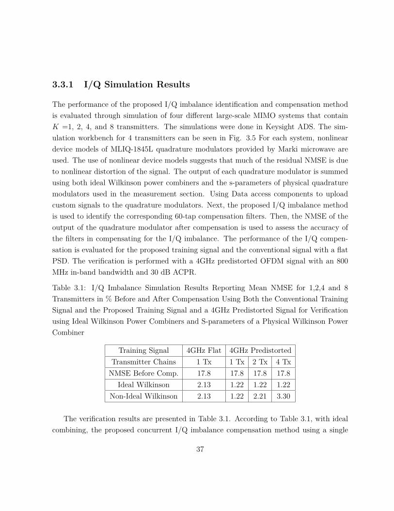
3.1 I/Q Imbalance Simulation Results Reporting Mean NMSE for 1,2,4 and 8Transmitters in % Before and After Compensation Using Both the Con-ventional Training Signal and the Proposed Training Signal and a 4GHzPredistorted Signal for Verification using Ideal Wilkinson Power Combinersand S-parameters of a Physical Wilkinson Power Combiner . . . . . . . . . 37

3.2 I/Q Imbalance Measurement Results Reporting NMSE for 1,2 and 4 Trans-mitters in % Before and After Compensation Using Both the ConventionalTraining Signal and the Proposed Training Signal and a 4GHz PredistortedSignal for Verification . . . . . . . . . . . . . . . . . . . . . . . . . . . . . . 42

3.3 DPD Linearization Measurement Results Reporting EVM in % for a mil-limetre wave (mmWave) PA Using an 800MHz OFDM Signal. . . . . . . . 43

viii

List of Figures

2.1 Generic complex signal to be generated. . . . . . . . . . . . . . . . . . . . 5

2.2 Block diagram of a quadrature modulator. . . . . . . . . . . . . . . . . . . 6

2.3 Ideal Quadrature modulation to generate signals at RF frequencies. . . . . 8

2.4 Quadrature modulation with I/Q imbalance when generating RF frequencies 9

2.5 Block diagram of the baseband model of a quadrature modulator. . . . . . 11

2.6 Block diagram of the baseband model of a quadrature modulator. . . . . . 11

2.7 Atmospheric absorption at different frequencies [1]. . . . . . . . . . . . . . 13

2.8 Digital Beamforming Architecture. . . . . . . . . . . . . . . . . . . . . . . 14

2.9 Analog Beamforming Architecture. . . . . . . . . . . . . . . . . . . . . . . 15

2.10 Hybrid Beamforming Architecture. . . . . . . . . . . . . . . . . . . . . . . 16

2.11 Massive MIMO System. . . . . . . . . . . . . . . . . . . . . . . . . . . . . 17

2.12 Single TOR single Tx . . . . . . . . . . . . . . . . . . . . . . . . . . . . . . 18

2.13 Multiple TOR . . . . . . . . . . . . . . . . . . . . . . . . . . . . . . . . . . 19

3.1 Block diagram for a mmWave MIMO transmitter system with K independenttransmit chains utilizing a single TOR for compensation. . . . . . . . . . . 22

3.2 (a) Block diagram of the I/Q compensator. (b) Block diagram of the base-band model of a quadrature modulator for a single transmitter chain. . . . 23

ix

3.3 Typical PSD of a predistorted signal at the input of a PA. . . . . . . . . . 28

3.4 PSD of proposed training signal vs conventional training signal. . . . . . . 36

3.5 Simulation workbench for the simulated verification of the proposed concur-rent I/Q imbalance identification and compensation scheme for four trans-mitter chains. . . . . . . . . . . . . . . . . . . . . . . . . . . . . . . . . . . 39

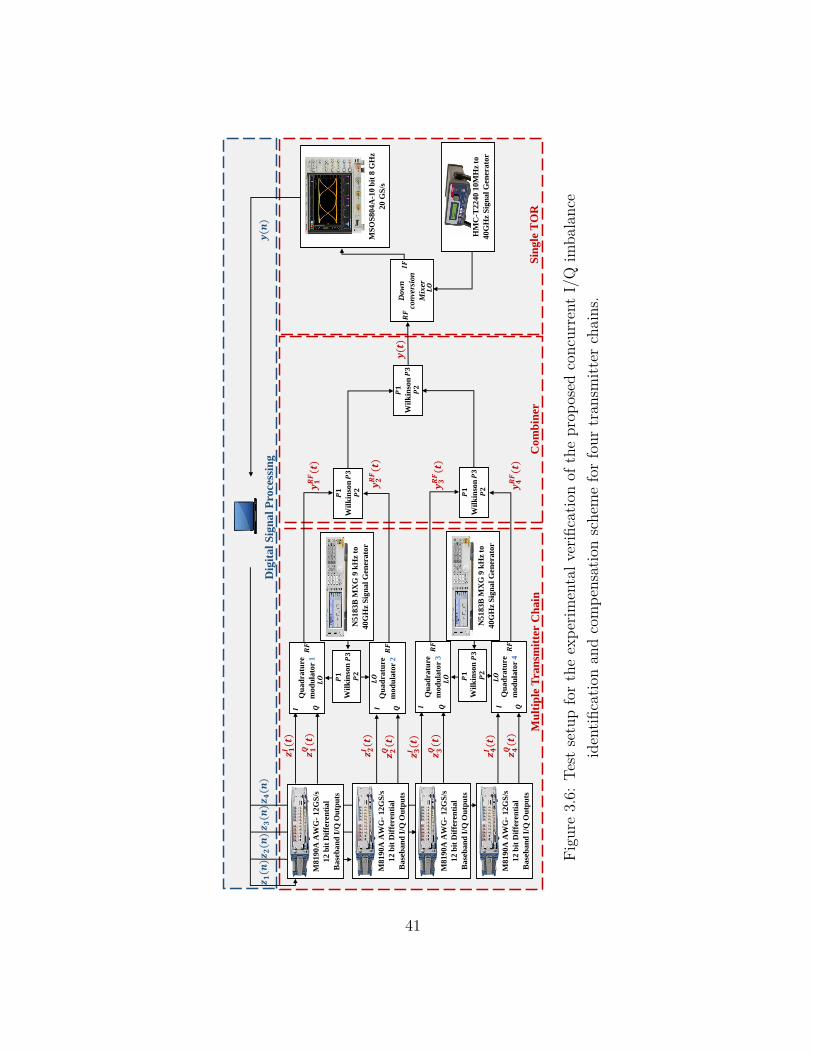
3.6 Test setup for the experimental verification of the proposed concurrent I/Qimbalance identification and compensation scheme for four transmitter chains. 41

3.7 Measured spectra of DPD with and without I/Q imbalance compensation. 44

x

Abbreviations

3G third generation 10

3GPP 3rd Generation Partnership Project 7

4G fourth generation 1, 10

5G fifth generation 1, 2, 4, 7, 12, 13, 18

ACPR adjacent channel power ratio 1, 13, 27, 35–37, 43

CRV complexity-reduced Volterra 43

DAC digital-to-analog converter 2, 4

DPD digital predistortion 7, 10, 11, 13, 18–20, 27, 35, 43

EVM error vector magnitude 1, 7, 13, 27, 35, 36, 43

FIR finite impulse response 22, 29

IIR infinite impulse response 26

IOT Internet of Things 1

LO local oscillator 6, 7, 40

xi

MIMO multiple-input multiple-output 1–3, 12, 18, 20–22, 37, 38

mmWave millimetre wave viii, 1–3, 12, 13, 16, 21, 35, 43

MSE mean squared error 28, 30, 32

NMSE normalized mean squared error 7, 36–38, 42

PA power amplifier 19, 20, 27, 35, 43

PSD Power Spectral Density 27, 28, 31, 34–37

RF radio frequency 21, 27, 40

SISO single input and single output 1, 4, 10, 18

SMDA spacial division multiple access 2, 12, 17

TOR transmitter observation receiver 18, 20, 21, 24, 35, 36, 38, 42

Tx transmitter 22

UWB ultra wideband 1, 2, 4, 13, 18

xii

List of Symbols

Im{·} Imaginary operator: denotes the imaginary component of a complex signals.

Re{·} Real operator: denotes the real component of a complex signals.

x Complex scalar: denoted in lowercase.

x Complex vector: represents a vector of complex scalars, i.e., [x(0), x(1), · · · , x(N)]T

denoted in bold lowercase.

X Complex matrix: represents a matrix of complex scalars denoted in bold uppercase.

H(z) Z-domain expression: denotes the z-transform of the impluse response h(n).

IN×N Identity matrix: denotes the identity matrix of size N ×N .

‖·‖2 L2 norm: denotes the L2 norm of a vector

xiii

Chapter 1

Introduction

Today’s fourth generation (4G) cellular mobile communication networks are tasked withthe heavy burden of the ever increasing number of mobile users and their demand for datafaster data rates. As new technologies are introduced, the fifth generation (5G) of cellularmobile communications will be required to manage enormous speeds to multiple times moredevices than 4G cellular networks. There are 5 technologies leading the way in enabling thefirst 5G networks. These are mmWave, massive multiple-input multiple-output (MIMO),beamforming, small cells, and full duplex [1], [2]. This thesis focuses on identifying andcompensating for transmitter hardware impairments in mmWave quadrature modulatorsmodulators for MIMO systems. The transition from sub 6GHz and single input and singleoutput (SISO) systems to mmWave and MIMO brings a new set of challenges that mustbe carefully considered when finding a solution to compensating for hardware impairmentsin upcoming 5G systems.

As technologies such as smart vehicles, smart transport and the Internet of Thingss(IOTs) become a reality, the need for bandwidth and available spectra increase. Thecurrent sub-6GHz frequency bands used for mobile communications do not have enoughbandwidth to support all emerging applications [1]. As a result, future 5G systems willutilize the mmWave frequency bands, enabling ultra wideband (UWB) signal transmission.Furthermore, new 5G standards for mmWave transmitters have strict error vector magni-tude (EVM) requirements; however, adjacent channel power ratio (ACPR) requirements

1

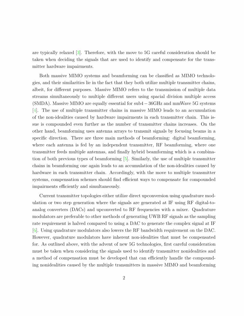
are typically relaxed [3]. Therefore, with the move to 5G careful consideration should betaken when deciding the signals that are used to identify and compensate for the trans-mitter hardware impairments.

Both massive MIMO systems and beamforming can be classified as MIMO technolo-gies, and their similarities lie in the fact that they both utilize multiple transmitter chains,albeit, for different purposes. Massive MIMO refers to the transmission of multiple datastreams simultaneously to multiple different users using spacial division multiple access(SMDA). Massive MIMO are equally essential for sub4−36GHz and mmWave 5G systems[4]. The use of multiple transmitter chains in massive MIMO leads to an accumulationof the non-idealities caused by hardware impairments in each transmitter chain. This is-sue is compounded even further as the number of transmitter chains increases. On theother hand, beamforming uses antenna arrays to transmit signals by focusing beams in aspecific direction. There are three main methods of beamforming: digital beamforming,where each antenna is fed by an independent transmitter, RF beamforming, where onetransmitter feeds multiple antennas, and finally hybrid beamforming which is a combina-tion of both previous types of beamforming [5]. Similarly, the use of multiple transmitterchains in beamforming one again leads to an accumulation of the non-idealities caused byhardware in each transmitter chain. Accordingly, with the move to multiple transmittersystems, compensation schemes should find efficient ways to compensate for compoundedimpairments efficiently and simultaneously.

Current transmitter topologies either utilize direct upconversion using quadrature mod-ulation or two step generation where the signals are generated at IF using RF digital-to-analog converters (DACs) and upconverted to RF frequencies with a mixer. Quadraturemodulators are preferable to other methods of generating UWB RF signals as the samplingrate requirement is halved compared to using a DAC to generate the complex signal at IF[6]. Using quadrature modulators also lowers the RF bandwidth requirement on the DAC.However, quadrature modulators have inherent non-idealities that must be compensatedfor. As outlined above, with the advent of new 5G technologies, first careful considerationmust be taken when considering the signals used to identify transmitter nonidealities anda method of compensation must be developed that can efficiently handle the compound-ing nonidealities caused by the multiple transmitters in massive MIMO and beamforming

2

systems.

This thesis is organized into the following chapters, First, in Chapter 2, the backgroundtheory on quadrature modulators and their inherent I/Q imbalance is presented, this isfollowed by a literature review of the current I/Q compensation schemes. Afterwords, aliterature review of current 5G technologies is demonstrated. Chapter 2 ends with thebackground and literature review of I/Q imbalance compensation schemes in MIMO sys-tems. Chapter 3 presents the proposed method of compensating transmitter I/Q imbalancein mmWave MIMO systems as well as judiciously engineered training signals to be usedin the identification process. This chapter ends by validation of the method and trainingsignal in both simulation and measurement. Lastly, Chapter 4 outlines the conclusion andthe possible avenues for future work to be conducted.

3

Chapter 2

Background Theory

2.1 I/Q Imbalance in SISO Systems

In this section we begin by outlining the basics of I/Q imbalance effects in SISO systems andan overview of the literature on methods of I/Q imbalance identification and compensationare presented.

2.1.1 Overview of I/Q Imbalance

Quadrature modulators are used to generate complex signals at RF frequencies. Quadra-ture modulation are preferable to other methods of generating UWB RF signals as the datastreams are split into separate in-phase (real) and quadrature-phase (imaginary) compo-nents. Therefore, the sampling rate requirement on the DACs is halved compared to usinga DAC to generate the complex signal at IF [6], which would then be up-converted toRF frequencies by a mixer. Using quadrature modulators also lowers the RF bandwidthrequirement on the DAC. Therefore despite the introduction of RFDACs the ever increas-ing bandwidth requirements for 5G systems means quadrature modulators are still readilyused to generate UWB signals.

Lets say we have a generic complex signal [7] that we want to generate, as shown in

4

Fig. 2.1. This signal can be represented in rectangular form as,

x(t) = xI(t) + jxQ(t) (2.1)

This signal can also be represented in polar form as,

x(t) = |x(t)|ejθ(t) (2.2)

where|x(t)| =

√x2I(t) + x2

Q(t)

θ(t) = tan−1(xQ(t)xI(t)

)

𝑋 𝑓

𝑓 𝐵𝑊/2 𝐵𝑊/2

Figure 2.1: Generic complex signal to be generated.

Of course we cannot generate this signal at baseband since it is a complex signal. Togenerate this signal, we must do so using an RF carrier, i.e.,

xRF (t) = Re[x(t)ej2πfct]= Re[ |x(t)|ejθ(t)ej2πfct]= Re[ (xI(t) + jxQ(t))ej2πfct]= Re[ (xI(t) + jxQ(t))(cos2πfct+ jsin2πfct)]

xRF (t) = xI(t)cos2πfct− xQ(t)sin2πfct (2.3)

5

The block diagram of a quadrature modulator is shown in Fig. 2.2, it can be seenthat it preforms the operation shown in (2.3). In order to see the operation of quadraturemodulator clearly, it is best to demonstrate the operation in the frequency domain as shownin Fig. 2.3. It can be seen that the real (X(f)) and imaginary (X(f)) signals are combinedinto the original complex signal at the desired RF frequency. This operation is dependenton the ability of the physical quadrature modulator to emulate this ideal behaviour.

90°

DAC

DAC

𝑥𝐼(𝑡)

𝑥𝑄(𝑡)

cos 2𝜋𝑓𝑐𝑡

sin2𝜋𝑓𝑐𝑡

𝑥𝑅𝐹 𝑡

Figure 2.2: Block diagram of a quadrature modulator.

I/Q imbalance is detrimental to the ideal RF signal generation displayed in Fig. 2.3.I/Q imbalance arises from the physical components non-idealities and can be categorizedinto two effects. First, ideally, the I and Q paths must have identical phase and amplituderesponse which do not vary with frequency. In reality, however, this is not the case, and theamplitude and phase imbalance leads to improper combining of the I and Q components ofthe signal. Second, the hybrid 90◦ coupler used to drive the mixers with the local oscillator(LO) signals might not have perfect 90◦ phase offset between the two output ports meaningthe I and Q components will not be mixed with the proper cos2πfct and sin2πfct carriers.Once again, this offset will lead to non-ideal combining.

Fig. 2.4 displays the behaviour a physical quadrature modulator exhibits when itexhibits I/Q imbalance. In this example, instead of perfect 90◦ phase difference betweenthe two paths, the phase difference is 80◦, causing a 10◦ phase imbalance. There is also

6

an amplitude imbalance between the two paths with the I path having 3dB attenuationcompared to the Q path. Due to this I/Q imbalance we have unwanted gray and graydotted imaginary components in the up-converted signal shown in Fig. 2.4(e). We also seethat the real components have not cancelled properly with a red dashed residual signal onthe negative real axis. Clearly, without perfect amplitude and phase and balance betweenthe paths, there is a severe degradation in signal quality. In a practical RF system thistranslates to high EVM or normalized mean squared error (NMSE), for which there arestringent requirements in new 3rd Generation Partnership Project (3GPP) 5G standards[3]. Therefore, in the literature, I/Q imbalance compensation techniques have receivedsignificant attention.

2.1.2 Literature Review

In the literature, most I/Q imbalance identification and compensation schemes can bedivided into three categories. Frequency independent, frequency dependent and joint I/Qimbalance and digital predistortion (DPD) compensation schemes.

Frequency Independent

Frequency Independent I/Q imbalance compensation schemes consider the I/Q imbalanceto be a constant amplitude and phase offset that does not vary with frequency. Frequencyindependent I/Q imbalance effects are sometimes referred to as static I/Q imbalance. Theauthors in [8] analyze the static I/Q imbalance effects and provides a quantitative assess-ment of the losses. The authors then present adaptive compensation techniques for thequadrature modulator at both the transmitter and receiver. Similarly, the authors in [9]present an adaptive I/Q imbalance compensator which estimates and separates the respec-tive I/Q imbalances of the transmitter and receiver by utilizing a 90◦ shift in the LO. Thesesolutions are feasible in systems with smaller modulation bandwidths. As the data ratesof systems increases, leading to larger modulation bandwidths frequency independent I/Qimbalance compensation schemes become ever more impractical.

7

90°

DAC

DAC

𝑥𝐼(𝑡)

𝑥𝑄(𝑡)

cos 2𝜋𝑓𝑐𝑡

sin2𝜋𝑓𝑐𝑡

𝑥𝑅𝐹 𝑡

a

b

c

d

e

𝑓

𝑅𝑒 𝑋 𝑓

𝐼𝑚 𝑋 𝑓

a b

c

90°

-90°

𝑓

𝑅𝑒 𝑋 𝑓

𝐼𝑚 𝑋 𝑓

d

𝑓

𝑅𝑒 𝑋 𝑓

𝐼𝑚 𝑋 𝑓

𝑓

𝑅𝑒 𝑋 𝑓

𝐼𝑚 𝑋 𝑓

𝑓𝑐

𝑓𝑐

𝑓𝑐

𝑓𝑐

𝑓

𝑅𝑒 𝑋 𝑓

𝐼𝑚 𝑋 𝑓

𝑓𝑐

𝑓𝑐

e

Figure 2.3: Ideal Quadrature modulation to generate signals at RF frequencies.

8

90°

DAC

DAC

𝑥𝐼(𝑡)

𝑥𝑄(𝑡)

cos 2𝜋𝑓𝑐𝑡

sin2𝜋𝑓𝑐𝑡

𝑥𝑅𝐹 𝑡

a

b

d

d

e

𝑓

𝑅𝑒 𝑋 𝑓

𝐼𝑚 𝑋 𝑓

a b

c

90°

-90°

𝑓

𝑅𝑒 𝑋 𝑓

𝐼𝑚 𝑋 𝑓

d

𝑓

𝑅𝑒 𝑋 𝑓

𝐼𝑚 𝑋 𝑓

𝑓

𝑅𝑒 𝑋 𝑓

𝐼𝑚 𝑋 𝑓

𝑓

𝑅𝑒 𝑋 𝑓

𝐼𝑚 𝑋 𝑓

𝑓𝑐

𝑓𝑐

𝑓𝑐

𝑓𝑐

𝑓𝑐

𝑓𝑐

e

-80°

-80°

Figure 2.4: Quadrature modulation with I/Q imbalance when generating RF frequencies

9

Frequency Dependent

Third generation (3G) and 4G systems brought with them higher data rates and thereforeused greater modulation bandwidths to transmit signals. As the modulation bandwidthincreases beyond a few MHz frequency-dependent I/Q imbalance effects become moreimportant. It is no longer feasible to model the I/Q imbalance as a simple amplitudeand phase offset.

SISO I/Q imbalance compensation techniques have received significant attention [10],[11], [12], [13]. The first comprehensive model for I/Q imbalance was presented in [10]for quadrature IF radio receivers. The model, shown in Fig. 2.5, and covered in extensivedetail in Chapter 3, approximates the quadrature modulator as four real-valued FIR filters.This model is adopted in [11] and [12] for transmitters. In [11] the authors use a least-squares based time domain approach to identify and compensate for the I/Q imbalance.While the authors in [12] take a frequency domain approach and take advantage of thealiasing exhibited during sub-sampling in combination with multi-tone training signals toreduce the sampling rate during I/Q imbalance identification.The authors in [13] assumea similar model, shown in Fig. 2.6. However, when it came to compensation they onlycompensate for the effects of H2. The authors also present two estimation approaches, thefirst estimation approach stems from second-order statistics of complex communicationsignals, while the second technique is based on widely-linear least-squares model fitting.

These approaches cannot be directly generalized to large-scale MIMO systems. In fact,the increase in the number of quadrature modulators in MIMO systems brings a new setof challenges and trade-offs. Especially when considering that the I/Q imbalance not onlydeteriorates the error vector magnitude (EVM) of the output signal but is also detrimentalto the linearization of PAs using DPD [6].

10

𝑄

𝐼

𝒋

𝑄 ′

𝐼 ′ 𝒉𝒌𝟏𝟏

𝒉𝒌𝟐𝟏

𝒉𝒌𝟏𝟐

𝒉𝒌𝟐𝟐

𝐼 ′ + 𝑗𝑄 ′

Figure 2.5: Block diagram of the baseband model of a quadrature modulator.

𝐼 + 𝑗𝑄 𝐼 ′ + 𝑗𝑄 ′

𝑯𝟏 ∙ ∗

𝑯𝟐

Figure 2.6: Block diagram of the baseband model of a quadrature modulator.

Joint I/Q and DPD

In an effort to alleviate transmitters of both linear and nonlinear impairments. Manypublications propose joint I/Q imbalance and DPD compensation schemes. These includeextending the parallel Hammerstein structure [14], Volterra series model [15] and asym-metrical complexity-reduced Volterra series (CRV) model [16]. These methods, althoughcompact, suffer from an increase in computational complexity compared to independentI/Q compensation. This occurs because when any linear memory is present before thenon-linearity it significantly increases the linear memory order required in the DPD [17][18]. Overall, resulting in an exponential increase in the number of DPD coefficients neededto compensate the combined nonlinearity and I/Q imbalance.

11

2.2 5G Technologies

Although 5G systems are still in their early stages of development, 5 technologies haveemerged as front-runners in realizing 5G wireless networks [2]. These are mmWave, massiveMIMO, beamforming, small cells, and full duplex.

Massive MIMO and beamforming can both be categorized as subsets of MIMO systems.MIMO simply stands for mulitple-input multiple-output, which on the transmitter sideindicates the use of multiple transmitter chains. The difference between massive MIMOand beamforming can be summarized as follows, beamforming uses antenna arrays totransmit signals by focusing beams in a specific direction. In contrast, massive MIMOrefers to the transmission of multiple data streams simultaneously to multiple differentusers using SMDA.

This thesis tackles the problem of I/Q imbalance in mmWave MIMO systems. There-fore, in this section, a brief summary and literature review of mmWave, massive MIMOand beamforming systems demonstrates how the addition of multiple transmitter chains,and the specific architectures used in new 5G systems brings a new set of challenges andtrade-offs when correcting for transmitter hardware impairments, and specifically for ourcase, I/Q imbalance.

2.2.1 Millimeter Wave

As today’s cellular providers attempt to deliver higher data rates to an ever increasingnumber of users, they are limited to the frequency spectrum range below 6GHz [1]. Oneway to keep up with the demand is to move to the mmWave frequencies. There are variousdefinitions of the frequencies that are considered to be the mmWave. However, most articlesconsider the mmWave band to be between 24GHz and 300GHz [19], [20], [1], [21], [2]. Earlyresearch focused on the lower ends of mmWave frequencies due to atmospheric absorptioncharacteristics at frequencies such as 28GHz and 38GHz as can be seen in Fig.2.7 [1]. As aresult, the FCC recently auctioned off the 24GHz and 28GHz mmWave spectrum in early2019.

12

Moving to the mmWave frequencies opens a new portion of the spectrum for newsignals. As a result of the new-found availability of spectra, transmitters will be using largermodulation bandwidths in order to provide higher data rates [21], [1]. As a result, frequencydependent I/Q imbalance impairments will be more important than ever. Therefore, anyfuture I/Q imbalance identification and compensation schemes must be able to withstandthe large variations of hardware behavior over bandwidths in the 100s of MHz exhibitedby UWB signals. Moreover, new 5G standards for mmWave transmitters have strict EVMrequirements; however, ACPR requirements are typically relaxed [3]. Therefore, with themove to 5G careful consideration should be taken when deciding the signals that are used toidentify and compensate for the transmitter hardware impairments. These signals shouldprioritize the EVM minimization over ACPR minimization when applying DPD.

Figure 2.7: Atmospheric absorption at different frequencies [1].

2.2.2 Beamforming

Beamforming uses antenna arrays to transmit signals by focusing beams in a specific di-rection. There are three main methods of beamforming: digital beamforming, where eachantenna is fed by an independent transmitter, RF beamforming, where one transmitter

13

feeds multiple antennas, and finally hybrid beamforming which is a combination of bothprevious types of beamforming [5]. Each beamforming architecture has its benefits anddrawbacks, therefore they are utilized for applications[22].

𝑥1(𝑛) DAC PA

DACQuadrature Modulator 1

𝑥2(𝑛)

𝑥𝐾(𝑛)

Digital Beamformer

Digital Signal Processing RF Equipment

DAC PA

DACQuadrature Modulator 2

DAC PA

DACQuadrature Modulator K

Figure 2.8: Digital Beamforming Architecture.

Digital Beamforming

Digital beamforming uses multiple transmitter chains in conjunction with one antennaper chain to create one or multiple concentrated electromagnetic beams that are used totransmit data. The digital beamforming architecture is shown in Fig. 2.8. Due to thefact that phase shifting and implementation of different beamforming algorithms are donein the digital domain, digital beamforming systems can be designed to be single or multiuser. For example, in an 8 transmitter system, the first 4 and last 4 antennae can be usedto bidirectionally transmit a stream of information to different receivers. As a trade-off to

14

these degrees of freedom, and the increased hardware complexity, digital beamforming isa costly, high power, high complexity method of implementing directional transmission ofsignals. [22]. Due to the high cost of implementing a large amount of transmitter chains,digital beamforming architectures are usually reserved for sub-6GHz applications [23].

RF Equipment

𝑥1(𝑛) DAC PA

DACQuadrature Modulator 1𝑥2(𝑛)

Analog BeamformerDigital

Signal

Processing

PAPA

PA

Figure 2.9: Analog Beamforming Architecture.

Analog Beamforming

Analog beamforming uses a single transmitter chain in conjunction with analog phaseshifters which are connected to an antenna array to create a concentrated electromagneticbeam that is used to transmit data to a single user. The analog beamforming architecture isshown in Fig. 2.9. Analog beamforming systems are usually designed to serve one receiver.Analog beamforming is a cost effective, low power, low complexity method of implementingdirectional transmission of signals but suffers from lack of freedom in implementing differentbeamforming algorithms compared to digital and hybdrid beamforming [22].

15

𝑥1(𝑛) DAC PA

DACQuadrature Modulator 1

𝑥2(𝑛)

𝑥𝐾(𝑛) DAC PA

DACQuadrature Modulator K

DAC PA

DACQuadrature Modulator 2Digital

Beamformer

Digital Signal Processing RF Equipment

Analog Beamformer

Analog Beamformer

Analog Beamformer

Figure 2.10: Hybrid Beamforming Architecture.

Hybrid Beamforming

Hybrid beamforming is a combination of digital beamforming and analog beamforming.It uses both individual transmitter chains as well as analog phase shifters, as shown in2.10. This combination allows hybrid beamforming architectures to provide a compromisebetween the low complexity of analog beamforming and high degrees of freedom of digitalbeamforming. Therefore, hybrid beamforming architectures can have a large number ofantennas and also implement complex beamforming algorithms. Since mmWave systemshave higher path loss than sub-6GHz systems, large antenna gain, and therefore manyantennae, is required due to the increase in path loss, therefore, hybrid beamforming isused in most mmWave beamforming designs [20], [24]. Once again, since this architecturehas multiple transmitters, careful consideration should be taken in compensating for thecompounding non-idealities of each transmitter chain.

16

2.2.3 Massive MIMO

In massive MIMO, a multi-antenna transmitter transfers multiple streams of data at thesame frequency simultaneously to multiple receivers, as shown in Fig. 2.11. This is knownas SMDA, such a system has an input output relationship described by .

y = Hx, (2.4)

where

H =

h1,1 h1,2 · · · h1,M

... ... ...hK,1 hK,2 · · · hK,M

.The channel matrix, H can then be used to implement linear precoding techniques suchmaximum ratio transmission and zero-forcing [4]. There are also nonlinear signal process-ing techniques that offer higher capacity but are often difficult or highly computationallyintensive to implement[25]. Massive MIMO architectures are usually considered to be sub6GHz technologies [21].

RF

EquipmentDigital Signal

Processing

𝑥1(𝑛)

𝑥𝐾(𝑛)

𝑥2(𝑛)

Channel

RF User

Equipment

MIMO Precoder

1,2

1,𝑀

𝐾,1

𝐾,2

𝐾 ,𝑀

Tx

Tx

Tx

Figure 2.11: Massive MIMO System.

17

2.3 I/Q Imbalance in MIMO Systems

2.3.1 Overview of I/Q Imbalance in MIMO Systems

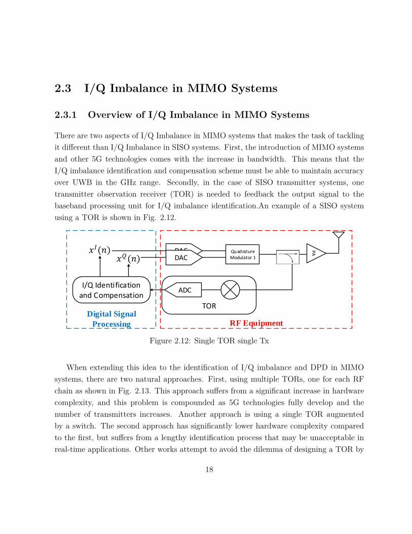
There are two aspects of I/Q Imbalance in MIMO systems that makes the task of tacklingit different than I/Q Imbalance in SISO systems. First, the introduction of MIMO systemsand other 5G technologies comes with the increase in bandwidth. This means that theI/Q imbalance identification and compensation scheme must be able to maintain accuracyover UWB in the GHz range. Secondly, in the case of SISO transmitter systems, onetransmitter observation receiver (TOR) is needed to feedback the output signal to thebaseband processing unit for I/Q imbalance identification.An example of a SISO systemusing a TOR is shown in Fig. 2.12.

TOR

RF EquipmentDigital Signal

Processing

I/Q Identification and Compensation

𝑥𝐼(𝑛) DAC PA

DACQuadrature Modulator 1𝑥𝑄(𝑛)

ADC

Figure 2.12: Single TOR single Tx

When extending this idea to the identification of I/Q imbalance and DPD in MIMOsystems, there are two natural approaches. First, using multiple TORs, one for each RFchain as shown in Fig. 2.13. This approach suffers from a significant increase in hardwarecomplexity, and this problem is compounded as 5G technologies fully develop and thenumber of transmitters increases. Another approach is using a single TOR augmentedby a switch. The second approach has significantly lower hardware complexity comparedto the first, but suffers from a lengthy identification process that may be unacceptable inreal-time applications. Other works attempt to avoid the dilemma of designing a TOR by

18

simply lumping the I/Q compensation with the channel estimation done on the receiverside. Examples of both categories of work are shown in the literature review section.

TOR

DAC PA

DACQuadrature Modulator K

Analog Beamformer

RF EquipmentDigital Signal

Processing

𝑥1(𝑛)

𝑥𝐾(𝑛)

TOR

DAC PA

DACQuadrature Modulator 2

Analog Beamformer

DAC PA

DACQuadrature Modulator 1

Analog Beamformer

TOR

Digital Beamformer𝑥2(𝑛)

I/Q Identification and Compensation

Figure 2.13: Multiple TOR

2.3.2 Literature Review

Transmitter Observation Receiver Based

Most approaches to solving the problem of I/Q imbalance in MIMO systems attempts tocombine and compensate the problem of power amplifier (PA) non-linearity and I/Q imbal-ance into joint I/Q imbalance and DPD compensation. The authors in [26] use a compositeneural network DPD model for joint mitigation of crosstalk, I/Q imbalance, and nonlin-

19

earity in MIMO Transmitters in their approach, they opt to use a single TOR augmentedby a switch. This approach has significantly lower hardware complexity compared to mul-tiple TORs, but suffers from a lengthy identification process that may be unacceptable inreal-time applications.The authors in [27] present models for joint mitigation of static I/Qimbalance and MIMO PA distortion at the transmitter and use multiple TORs, therebyincreasing hardware requirements. These compensation schemes suffer from a significantincrease in computational complexity compared to independent I/Q compensation. Thisoccurs because when the I/Q imbalance is not compensated before the non-linearity itsignificantly increases the linear memory order in the DPD [17] [18]. This increase leadsto an exponential increase in the number of DPD coefficients needed to compensate thecombined nonlinearity and I/Q imbalance.

No Transmitter Observation Receiver

To circumvent the I/Q imbalance identification and the underlying dilemma of choosingthe number of TORs, in [28],[29],[30] the I/Q imbalance is lumped into the channel esti-mation process on the receiver side, thereby avoiding the use of any TOR. This approachsignificantly reduces the hardware complexity, however, it adds increases the computationalburden on the receiver side. Moreover, the works in [28],[29],[30] have their limitations asthey neglect the nonlinearity exhibited by PAs in the transmit chains. This is crucial be-cause I/Q imbalance significantly affects the performance of the DPD [31] and moreover, ifDPD is not preformed properly, the I/Q imbalance is heavily distorted by the nonlinearityexhibited by the PA, therefore it cannot be easily estimated on the receiver end.

20

Chapter 3

Compensation of Transmitter I/QImbalance in Millimeter-wave MIMOSystems

3.1 I/Q Imbalance Identification and CompensationMethod for Transmitters in MIMO Systems

Fig. 3.1 shows the block diagram of a mmWave multi-user MIMO transmitter with a sin-gle TOR used to observe the combined output signal y(t) of the K direct-conversion radiofrequency (RF) chains. The combined output signal is used to identify and compensate forthe inherent frequency-dependent I/Q imbalance in each chain. Accordingly, this leavesthe challenge of separating the output signals’ envelopes from yRFk (t), for each modulator,from the combined output signal, y(t), in order to concurrently identify the correspondingI/Q imbalance. In this thesis, we first present the model of the single chain in Fig. 3.1 [10].Using this model we develop a method of identifying the I/Q imbalances for multiple trans-mitter chains. Finally, the I/Q imbalances are compensated for by calculating appropriatecompensators which offset the I/Q imbalance inherent in quadrature modulators.

21

Quadrature

modulator 1

Quadrature

modulator 2

Quadrature

modulator K

I/Q

Compensator 1

I/Q

Compensator 2

I/Q

Compensator K

𝑥1(𝑛)

𝑥2(𝑛)

𝑥𝐾(𝑛)

DAC

DAC

DAC

DAC

DAC

DAC

Digital Signal Processing

Single Observation

Receiver Training

𝑦1𝑅𝐹(𝑡)

𝑦2𝑅𝐹(𝑡)

𝑦𝐾𝑅𝐹(𝑡)

𝑦(𝑡)

𝑰

𝑸

𝑰

𝑸

𝑰

𝑸

𝑹𝑭

𝑹𝑭

𝑹𝑭

𝑳𝑶

𝑳𝑶

𝑳𝑶

MIMO Antenna

Array System

𝑳𝑶 𝑺𝒐𝒖𝒓𝒄𝒆

𝑧1𝐼(𝑡)

𝑧1𝑄

(𝑡)

𝑧2𝐼(𝑡)

𝑧2𝑄

(𝑡)

𝑧𝐾𝐼 (𝑡)

𝑧𝐾𝑄

(𝑡)

RF Equipment

𝑦(𝑛)

Single Chain

Figure 3.1: Block diagram for a mmWave MIMO transmitter system with K independenttransmit chains utilizing a single TOR for compensation.

3.1.1 I/Q Compensator and Quadrature Modulator Model

To formulate the I/Q imbalance compensation for MIMO systems, the model first proposedin [10] and adopted in [11] and [13], for a single chain transmitter (Tx) is adopted. Thediscrete baseband model of the single chain highlighted in Fig. 3.1 is shown in Fig. 3.2. Thequadrature modulator is modeled in discrete baseband by four real-valued finite impulseresponse (FIR) filters, h11

k , h21k , h12

k , and h22k , as shown in Fig. 3.2(b). The filters that

constitute the quadrature modulator are known as I/Q Imbalance filters. In the idealcase of no I/Q imbalance h21

k and h12k would be equal to zero while h11

k and h22k would be

single-tap FIR filters of zero phase and magnitude one. The I/Q compensator designed toachieve the ideal quadrature modulator behavior consists of four real-valued FIR filters,g11k , g21

k , g12k , and g22

k , as shown in Fig. 3.2(a). In the sections below we first outline howto estimate the I/Q imbalance filters in Fig. 3.2(b). Next, from those estimates we designthe compensation filters in Fig. 3.2(a) which will be applied to the original input signal

22

thereby cancelling the effect of the I/Q imbalance.

𝑥𝑘(𝑛)

𝑧𝑘𝑄(𝑛)

𝑧𝑘𝐼 (𝑛)

𝒈𝒌𝟐𝟐

𝑅𝑒{∙}

𝐼𝑚{∙}

𝑦𝑘(𝑛)

𝒋

(a) I/Q Compensator (b) Baseband Quadrature Modulator Model

𝑦𝑞 ,𝑘(𝑛)

𝑦𝑖 ,𝑘(𝑛)

𝒈𝒌𝟏𝟐

𝒈𝒌𝟐𝟏

𝒈𝒌𝟏𝟏 𝒉𝒌

𝟏𝟏

𝒉𝒌𝟐𝟏

𝒉𝒌𝟏𝟐

𝒉𝒌𝟐𝟐

Figure 3.2: (a) Block diagram of the I/Q compensator. (b) Block diagram of thebaseband model of a quadrature modulator for a single transmitter chain.

3.1.2 I/Q Imbalance Identification

For the kth quadrature modulator, the output yk(n), which is the discrete complex base-band version of yRFk (t) in Fig. 3.1, is related to the discrete baseband in-phase zIk(n) andquadrature zQk (n) inputs to the quadrature modulator by

yk(n) = zIk(n) ∗ hIk(n) + zQk (n) ∗ hQk (n), (3.1)

wherehIk(n) = h11

k (n) + jh21k (n) (3.2)

hQk (n) = h12k (n) + jh22

k (n) (3.3)

are the equivalent complex-valued I/Q imbalance filters. In order to compensate for theI/Q imbalance, we must first estimate hI

k and hQk . To accomplish this, we first express 3.1

in vector form asyk = ZI

khIk + ZQ

k hQk , (3.4)

23

whereyk = [yk(L− 1), · · · , yk(N − 1)]T

hIk = [hIk(0), · · · , hIk(L− 1)]T

hQk = [hQk (0), · · · , hQk (L− 1)]T

ZIk = Re{Zk}

ZQk = Im{Zk}

and

Zk =

zk(L− 1) zk(L− 2) · · · zk(0)zk(L) zk(L− 1) · · · zk(1)

... ... ...zk(N − 1) zk(N − 2) · · · zk(N − L)

.

In the above, L designates the length of the I/Q imbalance filters and N denotes thenumber samples of the input signal zk(n). As shown in Fig. 3.1, the use of a single TORcaptures the vector-summed outputs of all the quadrature modulators, i.e.,

y =K∑k=1

yk. (3.5)

Combining (3.3) and (3.5) we arrive at

y =K∑k=1

ZIkh

Ik + ZQ

k hQk . (3.6)

To identify the I/Q imbalance filters we use a least-squares estimate approach and definethe cost function as

J =∥∥∥∥∥y −

K∑k=1

(ZIkh

Ik + ZQ

k hQk )∥∥∥∥∥

2

. (3.7)

The minimum value of 3.7 is found by taking the partial derivative of 3.7 with respect toeach hI

k and hQk and equating the results to zero [32]. This yields the least-squares estimate

of the I/Q imbalance filters expressed below

h = (QTQ)−1QTy, (3.8)

where

24

Q =[ZI

1 ZQ1 · · · ZI

K ZQK

]

h =

hI1

hQ1...

hIK

hQK

.

3.1.3 I/Q Compensator Filter Calculation

With the I/Q imbalance filters h11k , h21

k , h12k and h22

k estimated, from 3.8 the correspondingI/Q compensation filters g11

k , g21k , g12

k and g22k must satisfy the z-domain expression below

(see [11] and Fig. 3.2):H11k (z) H12

k (z)H21

k (z) H22k (z)

G11k (z) G12

k (z)G21k (z) G22

k (z)

= I2×2. (3.9)

Multiplying both sides of 3.9 by the matrix, H22k (z) −H12

k (z)−H21

k (z) H11k (z)

,and applying the inverse z-transform, we obtain

hDk (n) ∗ g11k (n) = h22

k (n) (3.10)

hDk (n) ∗ g12k (n) = −h12

k (n) (3.11)

hDk (n) ∗ g21k (n) = −h21

k (n) (3.12)

hDk (n) ∗ g22k (n) = h11

k (n) (3.13)

where hDk (n) is the determinant:

hDk (n) = h11

k (n) ∗ h22k (n)− h12

k (n) ∗ h21k .(n) (3.14)

25

Rewriting (3.10) - (3.14) in matrix form,

h22k = HD

k g11k (3.15)

h12k = −HD

k g12k (3.16)

h21k = −HD

k g21k (3.17)

h11k = HD

k g22k , (3.18)

where

hijk = [hij

k (0), · · · , hijk (L− 1)]T

gijk = [gijk (0), · · · , gijk (M − 1)]T ,

for i, jε{1, 2}. In the above, L designates the length of the I/Q imbalance filters andHD

k is defined as the convolution matrix of hDk (n). The I/Q compensation filters, gijk ,that solve 3.15 - 3.18 may be very long or have infinite impulse response (IIR) and arethus limited to an appropriate length M that approximates the IIR solution. To identifythe I/Q compensation filters we use a least-squares estimate approach. The least-squaresestimates, g11

k , g21k , g12

k and g22k , of the I/Q compensation filter for each transmitter are

then found to be,g11k = (HD

k

THD

k )−1HDk

Th22k (3.19)

g12k = −(HD

k

THD

k )−1HDk

Th12k (3.20)

g21k = −(HD

k

THD

k )−1HDk

Th21k (3.21)

g22k = (HD

k

THD

k )−1HDk

Th11k . (3.22)

The compensation filters can now be applied before transmission as follows

zIk(n) = xIk(n) ∗ g11k (n) + xQk (n) ∗ g12

k (n) (3.23)

zQk (n) = xQk (n) ∗ g22k (n) + xIk(n) ∗ g21

k (n). (3.24)

26

3.2 Choice of Training Signal

In practical RF chains, the PA exhibits non-negligible non-linearity that would compro-mise the EVM and ACPR of the transmitted signal. Without compensation for this non-linearity, the occupied bandwidth at the output of such a PA is expanded compared tothe bandwidth of the original signal at the input. An expansion factor of 5x is common,i.e., a 100 MHz modulation bandwidth at the input of the RF chain would result in a 500MHz modulation bandwidth at the PA output. To compensate for the non-linearity of thePA, baseband DPD [17] is commonly applied before I/Q modulation to compensate forthe passband non-linearity of the PA. This DPD is also a nonlinear operation, and thusthe modulation bandwidth at the output of the predistorter is typically 5x that of theoriginal RF signal and the DPD operates at 5x the Nyquist sampling rate of the originalsignal. Nevertheless, as the DPD and PA nonlinearities cancel each other, resulting inlinear operation overall, the modulation bandwidth at the PA output after linearization isthen that of the original signal. This nonlinearity cancellation is critically dependent onthe accuracy of the quadrature modulation operation over the predistorted signal band-width [31]. Therefore, the I/Q imbalance identification and compensation must maintainacceptable accuracy over the entire bandwidth of the predistorted signal. i.e., the I/Qimbalance correction for an original modulated signal of 800 MHz should extend over abandwidth of 4 GHz.

In [11] compensation for out-of-band I/Q imbalance is not performed since it is as-sumed a well-designed quadrature modulator would achieve an image-rejection ratio of 40dB, therefore leaving the image caused by I/Q imbalance in the out-of-band region be-low the noise floor of the receiver. However, for many commercially available quadraturemodulators, this is not the case. By contrast, in [12] and [33], the I/Q imbalance cali-bration was conducted using a training signal with a flat Power Spectral Density (PSD)over the targeted predistortion bandwidth. Although this conventional approach providessignificant performance increase when compared to no I/Q compensation, it fails to takeinto account the specific spectral shape of the predistorted signals that arise from the usecases of DPD for PAs. Predistorted signals have most of their power concentrated withinthe original signal bandwidth (called the in-band) with spectral regrowth (of lower power

27

Figure 3.3: Typical PSD of a predistorted signal at the input of a PA.

spectral density) in adjacent bands. An example of such a pre-distorted signal can be seenin Fig. 3.3.

Therefore, a judiciously designed signal with a PSD that achieves optimal compensa-tion performance is beneficial. In the upcoming subsection, the training signal PSD thatminimizes the mean squared error (MSE) between i) the actual output of the physicalquadrature modulator and ii) the predicted output based on the estimated I/Q imbalancefilters, is found. Specifically, in the upcoming subsection, it is shown that for optimal com-pensation the training signal should be chosen such that its PSD is the same as the PSDat the output of the predistorter, such as the one shown in Fig. 3.3. It is of note that thisMSE evaluates the accuracy of the filter coefficients in predicting the systems true output

28

over the entire linearization bandwidth.

Finding the Ideal Training Signal

Consider a noiseless I/Q modulator system that has an input-output relation characterizedby,

y(n) = zI(n) ∗ hI(n) + zQ(n) ∗ hQ(n),

In the above, zI(n) and zQ(n) are the real and imaginary components of the input signaland the hI(n) and hQ(n) are FIR filters each containing K unknown complex taps. Thiscan be represented in vector form as,

[y(N), y(N − 1), · · · , y(K)]T ∆= y = Qh (3.25)

whereQ = [ZI ZQ]

h =hI

hQ

hI = [hI(0), · · · , hI(K − 1)]T

hQ = [hQ(0), · · · , hQ(K − 1)]T

ZI = Re{Z}

ZQ = Im{Z}

Z =

z(N) z(N − 1) · · · z(N −K + 1)

z(N − 1) z(N − 2) · · · z(N −K)... ... ...

z(K) z(K − 1) · · · z(1)

.

To estimate the coefficients in this system we use a training stage. Since K is usuallylarge for physical systems, we wish to estimate this system using only 2L < 2K coefficientsspecified by the vector

h =hI

hQ

, (3.26)

29

wherehI = [hI(0), · · · , hI(L− 1)]T

hQ = [hQ(0), · · · , hQ(L− 1)]T .

The goal is to determine the training signal to be used in the estimation of h that minimizesthe MSE between the actual output of the system generated by the physical quadra-ture modulator during the verification stage, yve = [yve(N), yve(N − 1), · · · , yve(K)]T

and our prediction of the output based on the calculated I/Q imbalance filters, yve =[yve(N), yve(N − 1), · · · , yve(K)]T , i.e., to minimize

J = ‖yve − yve‖2 , (3.27)

whereyve = Qveh (3.28)

yve = Qveh (3.29)

andQve = [ZI

ve ZQve]

Qve = [ZIve ZQ

ve]

ZIve = Re{Zve}

ZQve = Im{Zve}

ZI

ve = Re{Zve}

ZQ

ve = Im{Zve}

Zve =

zve(N) zve(N − 1) · · · zve(N −K + 1)

zve(N − 1) zve(N − 2) · · · zve(N −K)... ... ...

zve(K) zve(K − 1) · · · zve(1)

Zve =

zve(N) zve(N − 1) · · · zve(N − L+ 1)

zve(N − 1) zve(N − 2) · · · zve(N − L)... ... ...

zve(K) zve(K − 1) · · · zve(K − L+ 1)

,

30

where Re{zve(n)} and Im{zve(n)} are the real and imaginary components of a zero-meanwide-sense stationary ergodic verification signal that is used to verify the efficacy of ourestimation of h. Substituting 3.28 and 3.29 into 3.27 we arrive at the cost function,

J =∥∥∥Qveh− Qveh

∥∥∥2, (3.30)

We now show that 3.30 can be minimized if the estimate h ÌĆ is calculated during thetraining phase using a training signal, ztr(n), that has the same second order statistics, orequivalently the same PSD, as the verification signal zve(n). We do this by representing3.30 in terms of the second order statistics of both the training and verification signals,then deriving the minimum solution. We begin by first identifying the estimate h in termsof the second order statistics of the training signal ztr(n). To estimate h we use a trainingstage characterized by the input-output relationship,

[ytr(N), ytr(N − 1), · · · , ytr(K)]T ∆= ytr = Qtrh (3.31)

whereQ = [ZI

tr ZQtr]

ZItr = Re{Ztr}

ZQtr = Im{Ztr}

Ztr =

ztr(N) ztr(N − 1) · · · ztr(N −K + 1)

ztr(N − 1) ztr(N − 2) · · · ztr(N −K)... ... ...

ztr(K) ztr(K − 1) · · · ztr(1)

.

and Re{ztr(n)} and Im{ztr(n)} are the real and imaginary components of the zero-meanwide-sense stationary ergodic training signal that is used to estimate h. Since the systemis to be identified using 2L < 2K coefficents, the least-squares estimate of these coefficientsfrom ytr is,

h = (QTtrQtr)−1QT

trytr (3.32)

whereQtr = [ZI

tr ZQtr]

31

ZItr = Re{Ztr}

ZQtr = Im{Ztr}

Ztr =

ztr(N) ztr(N − 1) · · · ztr(N − L+ 1)

ztr(N − 1) ztr(N − 2) · · · ztr(N − L)... ... ...

ztr(K) ztr(K − 1) · · · ztr(K − L+ 1)

.

Substituting 3.31 into 3.32 we arrive at

h = (QTtrQtr)−1QT

trQtrh (3.33)

For very large N , the second order statistics of an autocorrelation ergodic WSS signalconverge to the ensemble ones. This means that, for very large N , we can represent theestimate h in terms of the second order statistics of the real and imaginary part of thetraining signal. Let,

rabtr (u,N) = 1N

N−u∑n=0

zatr(n)zbtr(n+ u).

where a, bÏţ{I,Q}.Then as N →∞,

rabtr (u,N)→ E{ratr(n)rbtr(n+ u)} = rabtr (u),

where, convergence is in the MSE sense, and rabtr (u) is the cross-correlation function ofztr

a(n) and ztrb(n).Therefore, 3.33 converges to

h = R−1tr Rtrh, (3.34)

where

Rtr =RII

tr RIQtr

RQItr RQQ

tr

Rtr =

RIItr RIQ

tr

RQItr RQQ

tr

Rabtr =

rabtr (0) rabtr (1) · · · rabtr (L− 1)rabtr (1) rabtr (0) · · · rabtr (L− 2)

... ... ...rabtr (L− 1) rabtr (L− 2) · · · rabtr (0)

.

32

Rabtr =

Rabtr

rabtr (L) rabtr (L− 1) · · · rabtr (K − 1)rabtr (L− 1) rabtr (L− 2) · · · rabtr (K − 2)

... ... ...rabtr (1) rabtr (2) · · · rabtr (K − L)

.

and a, bÏţ{I,Q}.Rtr and Rtr represent the joint second-order statistics of zItr(n) and zQtr(n).Letting,

B = R−1tr Rtr (3.35)

we arrive ath = Bh (3.36)

Expanding the cost function in 3.30 and substituting 3.36 we arrive at 3.37,

J = (Qveh− Qveh)H(Qveh− Qveh)

= hHQTveQveh− 2hHQT

veQveh + hHQTveQveh

= hHQTveQveh− 2hHBT QT

veQveh + hHBT QTveQveBh (3.37)

Once again, for very large N , we can express the cost function in terms of the joint second-order statistics of the verification signal, zIve(n) and zQve(n).Let,

rabve(u) = E{rave(n)rbve(n+ u)},

and a, bÏţ{I,Q}.Then for very large N , the cost function in 3.37 converges to

J = hHRveh− 2hHBT Rveh + hHBT RveBh (3.38)

where

Rve =RII

ve RIQve

RQIve RQQ

ve

Rve =

RIIve RIQ

ve

RQIve RQQ

ve

Rve =

RIIve RIQ

ve

RQIve RQQ

ve

33

Rabve =

rabve(0) rabve(1) · · · rabve(K − 1)rabve(1) rabve(0) · · · rabve(K − 2)

... ... ...rabve(K − 1) rabve(K − 2) · · · rabve(0)

.

Rabve =

rabve(0) rabve(1) · · · rabve(L− 1)rabve(1) rabve(0) · · · rabve(L− 2)

... ... ...rabve(L− 1) rabve(L− 2) · · · rabve(0)

.

Rabve =

Rabve

rabve(L) rabve(L− 1) · · · rabve(K − 1)rabve(L− 1) rabve(L− 2) · · · rabve(K − 2)

... ... ...rabve(1) rabve(2) · · · rabve(K − L)

.

and a, bÏţ{I,Q}.Now that we have the cost function expressed in terms of the second orderstatistics of the training and verification signals, we find the B that minimizes the costfunction in 3.38. Differentiating 3.38 with respect to B [34], and equating to zero gives,

RveBhhH = RvehhH . (3.39)

One solution to 3.39 isB = R

−1ve Rve,

or in other words, from 3.35R

−1tr Rtr = R

−1ve Rve,

To satisfy the above we can chooseRtr = Rve

Rtr = Rve

i.e., we choose the real and imaginary parts of ztr(n) and zve(n) to have the same second-order statistics. Equivalently, the complex signals must have the same PSD.

Therefore, in this thesis, a training signal is carefully devised to mimic the spectral shapeof a pre-distorted signal, and thus occupies the entire compensation bandwidth. This choice

34

of training signal provides higher SNR for the in-band portion than the conventional choice,thereby increasing the accuracy of the compensation filter coefficients in the in-band whilestill calibrating for the adjacent spectral bands. If a flat PSD over the target linearizationbandwidth is adopted for the training signal, then the I/Q imbalance is estimated withequal accuracy over the entire band. Our choice of training signal decreases EVM withonly a slight sacrifice in ACPR at the PA output after linearization as compared to thecase where I/Q imbalance identification is conducted using a training signal with a flatPSD. This is advantageous as in mmWave communication applications, where the ACPRrequirements are relaxed compared to EVM. To generate a training signal with the samePSD as that of a predistorted signal we use a memoryless polynomial. The order of thepolynomial, P, is set so that it is the same as the order of the DPD that is to be used inthe system. The coefficients, cp, are also chosen to achieve similar ACPR to the PSD ofthe nonlinearity produced by the PA in the system. This ensures the PSD of the trainingsignal comes as close as possible to the PSD of the signal it is being applied to withoutknowing the exact signal a priori, i.e.,

zk(n) =P∑p=1

cpuk(n)|uk(n)|p. (3.40)

In the above, uk(n) are independently generated OFDM signals. Therefore, the trainingsignals,zk(n), for each transmitter are uncorrelated. In the next section, the performanceincrease of the proposed signal compared to that of the conventional signal is presented.

An example of the PSD of a training signal designed for I/Q compensation of a mmWavemodulator is shown in Fig. 3.4. In this example, the PA non-linearity is assumed togenerate spectral regrowth of 30 dBc below that of the in-band PSD. Thus, the trainingsignal in Fig. 3.4 has an adjacent band PSD that is 30 dB below that of the in-band PSD.Fig. 3.4 also shows a conventional flat PSD training signal with identical total power.

3.3 Simulation and Measurement Results

In this section, we examine the performance of the concurrent I/Q imbalance compensationmethod using a single TOR. We show that the concurrent compensation method maintains

35

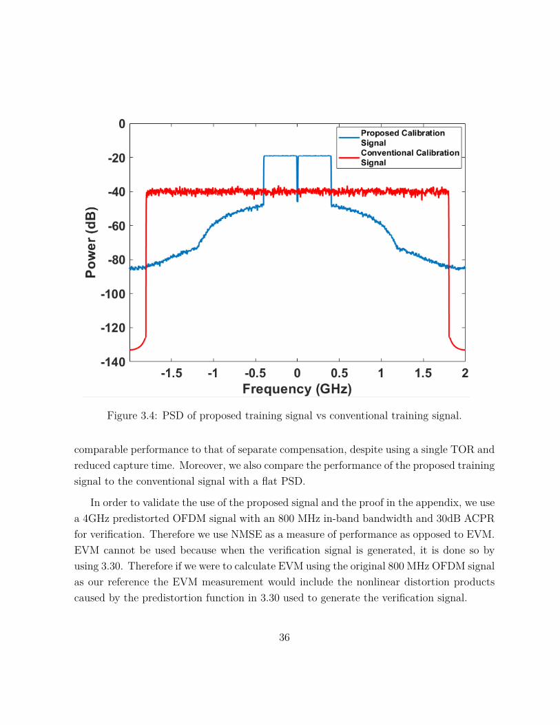
Figure 3.4: PSD of proposed training signal vs conventional training signal.

comparable performance to that of separate compensation, despite using a single TOR andreduced capture time. Moreover, we also compare the performance of the proposed trainingsignal to the conventional signal with a flat PSD.

In order to validate the use of the proposed signal and the proof in the appendix, we usea 4GHz predistorted OFDM signal with an 800 MHz in-band bandwidth and 30dB ACPRfor verification. Therefore we use NMSE as a measure of performance as opposed to EVM.EVM cannot be used because when the verification signal is generated, it is done so byusing 3.30. Therefore if we were to calculate EVM using the original 800 MHz OFDM signalas our reference the EVM measurement would include the nonlinear distortion productscaused by the predistortion function in 3.30 used to generate the verification signal.

36

3.3.1 I/Q Simulation Results

The performance of the proposed I/Q imbalance identification and compensation methodis evaluated through simulation of four different large-scale MIMO systems that containK =1, 2, 4, and 8 transmitters. The simulations were done in Keysight ADS. The sim-ulation workbench for 4 transmitters can be seen in Fig. 3.5 For each system, nonlineardevice models of MLIQ-1845L quadrature modulators provided by Marki microwave areused. The use of nonlinear device models suggests that much of the residual NMSE is dueto nonlinear distortion of the signal. The output of each quadrature modulator is summedusing both ideal Wilkinson power combiners and the s-parameters of physical quadraturemodulators used in the measurement section. Using Data access components to uploadcustom signals to the quadrature modulators. Next, the proposed I/Q imbalance methodis used to identify the corresponding 60-tap compensation filters. Then, the NMSE of theoutput of the quadrature modulator after compensation is used to assess the accuracy ofthe filters in compensating for the I/Q imbalance. The performance of the I/Q compen-sation is evaluated for the proposed training signal and the conventional signal with a flatPSD. The verification is performed with a 4GHz predistorted OFDM signal with an 800MHz in-band bandwidth and 30 dB ACPR.

Table 3.1: I/Q Imbalance Simulation Results Reporting Mean NMSE for 1,2,4 and 8Transmitters in % Before and After Compensation Using Both the Conventional TrainingSignal and the Proposed Training Signal and a 4GHz Predistorted Signal for Verificationusing Ideal Wilkinson Power Combiners and S-parameters of a Physical Wilkinson PowerCombiner

Training Signal 4GHz Flat 4GHz PredistortedTransmitter Chains 1 Tx 1 Tx 2 Tx 4 Tx

NMSE Before Comp. 17.8 17.8 17.8 17.8Ideal Wilkinson 2.13 1.22 1.22 1.22

Non-Ideal Wilkinson 2.13 1.22 2.21 3.30

The verification results are presented in Table 3.1. According to Table 3.1, with idealcombining, the proposed concurrent I/Q imbalance compensation method using a single

37

TOR achieved the same mean compensation accuracy for MIMO systems containing 1Table3.1, 2, 4 and 8 transmitters. The application of their compensation filter allowed forthe reduction of the mean NMSE from 17.8% to 1.22%However, from row 3 in Table3.1 we can see a progressive decrease in performance using the s-parameters of physicalWilkinson power combiners. This is due to the lack of isolation between the ports which iscompounded by increasing the number of Wilkinson power combiners. From simulation, wefind that the performance of the I/Q compensation method can be brought closer to thatof Table 3.1 if the isolation between the Wilkinson power combiner ports is kept below therealistic value of -20 dB, compared to the current -11.0dB (combination of S(2,1), S(3,1)and S(4,1)) and -17.5dB for 4Tx and 2Tx, respectively.

In addition, from Table 3.1, it can be seen that the proposed training signal offers betterperformance than that of the conventional training signal. Also, as shown in Table 3.1,these results are very close to those obtained using a dedicated observation receiver foreach transmitter channel and also match the measurement results presented in the nextsection.

38

DA

CD

CD

AC

DA

C

EN

VE

LO

PE

DA

C

DA

CD

AC

1

2

3S3P

DA

CD

AC

1

2

3S3P

1

2

3S3P

Q I

RL

Q I

RL

Q I

RL

Q I

RL

Va

rE

qn

Va

rE

qnV

ar

Eq

n

Va

rE

qn

Va

rE

qn

Sn

P

Sn

P

Da

taA

cce

ssC

om

po

ne

nt

Da

taA

cce

ssC

om

po

ne

nt

VA

R

Sn

P

V_

1To

ne

ML

IQ-1

84

5L

CH

V_

DC

V_

1To

ne

V_

DC

V_

DC

Da

taA

cce

ssC

om

po

ne

nt

ML

IQ-1

84

5L

CH

V_

1To

ne

ML

IQ-1

84

5L

CH

V_

DC

V_

DC

VA

R

VA

R

Da

taA

cce

ssC

om

po

ne

nt

V_

1To

ne

V_

DC

Da

taA

cce

ssC

om

po

ne

nt

V_

DC

En

velo

pe

Da

taA

cce

ssC

om

po

ne

nt

I_P

rob

e

VA

R

ML

IQ-1

84

5L

CH

DC

V_

DC

Da

taA

cce

ssC

om

po

ne

nt

VA

R

R

Da

taA

cce

ssC

om

po

ne

nt

Sn

P4

Sn

P1

DA

C8

DA

C7 V

AR

5

Sn

P2

SR

C1

3

SR

C1

2

X4S

RC

10

X3S

RC

11

DA

C4

SR

C8

DA

C5

SR

C9

SR

C7

X2S

RC

6

SR

C5

DA

C6

DA

C2

SR

C3

SR

C4

En

v3

VA

R4

VA

R1

X1

VA

R3

DC

1

SR

C2

DA

C1 V

AR

2

R2

DA

C3

I_P

rob

e1

iVa

l1=

tim

eiV

ar1

="t

ime

"E

xtra

pM

od

e=

Inte

rpo

latio

n M

od

eIn

terp

Do

m=

Re

cta

ng

ula

rIn

terp

Mo

de

=L

ine

ar

Typ

e=

Tim

e-d

om

ain

Wa

vefo

rmF

ile=

"D:\

Use

rs\h

23

rash

i\D

eskto

p\C

al_

ne

w\Q

_co

mp

_4

tx4

.tim

"

iVa

l1=

tim

eiV

ar1

="t

ime

"E

xtra

pM

od

e=

Inte

rpo

latio

n M

od

eIn

terp

Do

m=

Re

cta

ng

ula

rIn

terp

Mo

de

=L

ine

ar

Typ

e=

Tim

e-d

om

ain

Wa

vefo

rmF

ile=

"D:\

Use

rs\h

23

rash

i\D

eskto

p\C

al_

ne

w\I_

co

mp

_4

tx4

.tim

"

Q4

=file

{DA

C8

, "v

olta

ge

"}I4

=file

{DA

C7

, "v

olta

ge

"}

iVa

l1=

tim

eiV

ar1

="t

ime

"E

xtra

pM

od

e=

Inte

rpo

latio

n M

od

eIn

terp

Do

m=

Re

cta

ng

ula

rIn

terp

Mo

de

=L

ine

ar

Typ

e=

Tim

e-d

om

ain

Wa

vefo

rmF

ile=

"D:\

Use

rs\h

23

rash

i\D

eskto

p\C

al_

ne

w\Q

_co

mp

_4

tx3

.tim

"

Fre

q=

RF

fre

q

iVa

l1=

tim

eiV

ar1

="t

ime

"E

xtra

pM

od

e=

Inte

rpo

latio

n M

od

eIn

terp

Do

m=

Re

cta

ng

ula

rIn

terp

Mo

de

=L

ine

ar

Typ

e=

Tim

e-d

om

ain

Wa

vefo

rm

V=

po

lar(

sq

rt(P

_L

O),

0)

Fre

q=

RF

fre

qV

=p

ola

r(sq

rt(P

_L

O),

0)

Vd

c=

Q3

/7

File

="D

:\U

se

rs\h

23

rash

i\D

eskto

p\C

al_

ne

w\I_

co

mp

_4

tx2

.tim

"

iVa

l1=

tim

e

Typ

e=

Tim

e-d

om

ain

Wa

vefo

rmF

ile=

"D:\

Use

rs\h

23

rash

i\D

eskto

p\C

al_

ne

w\I_

co

mp

_4

tx3

.tim

"

Vd

c=

Q4

/7

Inte

rpM

od

e=

Lin

ea

r

iVa

r1=

"tim

e"

Ext

rap

Mo

de

=In

terp

ola

tio

n M

od

e

Vd

c=

I4/7

Ext

rap

Mo

de

=In

terp

ola

tio

n M

od

eIn

terp

Do

m=

Re

cta

ng

ula

r

Vd

c=

I3/7

Fre

q=

RF

fre

qV

=p

ola

r(sq

rt(P

_L

O),

0)

Vd

c=

Q2

/7

Vd

c=

I2/7

I3=

file

{DA

C5

, "v

olta

ge

"}

iVa

r1=

"tim

e"

V=

po

lar(

sq

rt(P

_L

O),

0)

Fre

q=

RF

fre

q

Vd

c=

Q1

/7

Q3

=file

{DA

C6

, "v

olta

ge

"}

iVa

l1=

tim

e

Typ

e=

Tim

e-d

om

ain

Wa

vefo

rmIn

terp

Mo

de

=L

ine

ar

Inte

rpD

om

=R

ecta

ng

ula

rE

xtra

pM

od

e=

Inte

rpo

latio

n M

od

eiV

ar1

="t

ime

"iV

al1

=tim

e

Inte

rpM

od

e=

Lin

ea

rIn

terp

Do

m=

Re

cta

ng

ula

r

Typ

e=

Tim

e-d

om

ain

Wa

vefo

rm

I2=

file

{DA

C4

, "v

olta

ge

"}Q

2=

file

{DA

C3

, "v

olta

ge

"}

Fre

q[1

]=R

Ffr

eq

Ord

er[

1]=

3S

top

=ts

top

Ste

p=

tste

p

Q1

=file

{DA

C2

, "v

olta

ge

"}

tste

p=

1/f

sV

ref=

1fs

=4

e9

tsto

p=

2.5

60

0e

-06

P_

LO

=1

7P

_R

F=

1V

dc=

I1/7

iVa

l1=

tim

eiV

ar1

="t

ime

"E

xtra

pM

od

e=

Inte

rpo

latio

n M

od

eIn

terp

Do

m=

Re

cta

ng

ula

rIn

terp

Mo

de

=L

ine

ar

Typ

e=

Tim

e-d

om

ain

Wa

vefo

rmF

ile=

"D:\

Use

rs\h

23

rash

i\D

eskto

p\C

al_

ne

w\I_

co

mp

_4

tx1

.tim

"

I1=

file

{DA

C1

, "v

olta

ge

"}

R=

50

Oh

m

File

="D

:\U

se

rs\h

23

rash

i\D

eskto

p\C

al_

ne

w\Q

_co

mp

_4

tx1

.tim

"

RF

fre

q=

28

GH

z

File

="D

:\U

se

rs\h

23

rash

i\D

eskto

p\C

al_

ne

w\Q

_co

mp

_4

tx2

.tim

"

Test

Figu

re3.

5:Si

mul

atio

nwo

rkbe

nch

for

the

simul

ated

verifi

catio

nof

the

prop

osed

conc

urre

ntI/

Qim

bala

nce

iden

tifica

tion

and

com

pens

atio

nsc

hem

efo

rfo

urtr

ansm

itter

chai

ns.

39

3.3.2 I/Q Measurement Results

In the following section, the proposed I/Q imbalance identification and compensationmethod is evaluated using the test setup shown in Fig. 3.6. In this setup, the I andQ components of four independent signals are generated using four arbitrary waveformgenerators (M8190A from Keysight Technology). These signals are fed to two I/Q mixers(MLIQ-1845 from Marki) for quadrature modulation. The LO signals are generated usingtwo analog signal generators (N5183B from Keysight Technology). The RF signals at theoutput of the four I/Q mixers, y1(t), y2(t), y3(t) and y4(t) are centered at 28GHz. Thesefour signals are then combined using three Wilkinson power combiners (two PD-0434SMand one PD-0140 from Marki) to yield the feedback signal needed to identify the I/Q im-balance of the two I/Q mixers. This feedback signal is first fed to the down conversionmixer (MM1-1140H from Marki). The LO signal needed by the down-conversion mixer isgenerated using a signal generator (HMC-T2240 from Hittite). The intermediate frequencysignal, centered around 3 GHz, is subsequently captured using a 10-bit 8GHz bandwidthhigh-speed oscilloscope (MSOS804A from Keysight Technology).

40

MS

OS

80

4A

-10

bit

8 G

Hz

20

GS

/s

Do

wn

con

vers

ion

Mix

er𝑳𝑶

𝑹𝑭

𝑰𝑭

HM

C-T

22

40

10

MH

z to

40G

Hz

Sig

nal

Gen

erato

r

Sin

gle

TO

RM

ult

iple

Tra

nsm

itte

r C

ha

in

Dig

ita

l S

ign

al

Pro

cess

ing

𝒛𝟐(𝒏)

𝒛𝟏(𝒏)

𝒚(𝒏)

M8

190A

AW

G-

12

GS

/s

12 b

it D

iffe

ren

tia

l

Base

ban

d I

/Q O

utp

uts

M8

190A

AW

G-

12

GS

/s

12 b

it D

iffe

ren

tia

l

Base

ban

d I

/Q O

utp

uts

Co

mb

iner

Qu

ad

ratu

re

mod

ula

tor

3

𝑰 𝑸𝑹𝑭

𝑳𝑶

N518

3B

MX

G 9

kH

z to

40

GH

z S

ign

al

Gen

era

tor

𝑷𝟏

𝑷𝟐

𝑷𝟑

Wil

kin

son

𝒚𝟑𝑹𝑭(𝒕)

𝒚𝟒𝑹𝑭(𝒕)

𝒛𝟑𝑰(𝒕)

𝒛𝟑𝑸(𝒕)

𝒛𝟒𝑰(𝒕)

𝒛𝟒𝑸(𝒕)

𝑷𝟏

𝑷𝟐

𝑷𝟑

Wil

kin

son

Qu

ad

ratu

re

mod

ula

tor

4

𝑰 𝑸𝑹𝑭

𝑳𝑶

Qu

ad

ratu

re

mod

ula

tor

1

𝑰 𝑸𝑹𝑭

𝑳𝑶

N518

3B

MX

G 9

kH

z to

40G

Hz

Sig

nal

Gen

erato

r

𝑷𝟏

𝑷𝟐

𝑷𝟑

Wil

kin

son

𝒚𝟏𝑹𝑭(𝒕)

𝒚𝟐𝑹𝑭(𝒕)

𝒛𝟏𝑰(𝒕)

𝒛𝟏𝑸(𝒕)

𝒛𝟐𝑰(𝒕)

𝒛𝟐𝑸(𝒕)

𝑷𝟏

𝑷𝟐

𝑷𝟑

Wil

kin

son

𝒚(𝒕)

Qu

ad

ratu

re

mod

ula

tor

2

𝑰 𝑸𝑹𝑭

𝑳𝑶

𝑷𝟏

𝑷𝟐

𝑷𝟑

Wil

kin

son

𝒛𝟑(𝒏)𝒛𝟒(𝒏)

M81

90A

AW

G-

12

GS

/s

12 b

it D

iffe

ren

tial

Base

ban

d I

/Q O

utp

uts

M8

190A

AW

G-

12

GS

/s

12 b

it D

iffe

ren

tia

l

Base

ban

d I

/Q O

utp

uts

Figu

re3.

6:Te

stse

tup

for

the

expe

rimen

talv

erifi

catio

nof

the

prop

osed

conc

urre

ntI/

Qim

bala

nce

iden

tifica

tion

and

com

pens

atio

nsc

hem

efo

rfo

urtr

ansm

itter

chai

ns.

41

Table 3.2: I/Q Imbalance Measurement Results Reporting NMSE for 1,2 and 4 Transmit-ters in % Before and After Compensation Using Both the Conventional Training Signaland the Proposed Training Signal and a 4GHz Predistorted Signal for Verification

Training Signal 4GHz Flat 4GHz PredistortedTransmitter Chains 1 Tx 1 Tx 2 Tx 4 Tx

NMSE Before Comp. 19.0 19.0 19.0 19.0NMSE After 20-tap 3.86 2.36 2.53 3.98NMSE After 60-tap 3.39 1.99 2.25 3.39NMSE After 120-tap 3.36 1.63 2.16 3.29

The performance of the concurrent compensation for 2 and 4 transmitter chains enabledsimultaneously is then compared to that of separate compensation, whereby all chains butone are turned off and the performance of the single chain is examined independently ofall other transmitters. This is done with both the conventional and proposed trainingsignals. Here, the capture time of the concurrent method is fixed to be the same as thatfor compensation of a single transmitter chain in the sequential method. In other words,for K transmitter chains, the proposed method requires K times less capture time.

The result from this verification experiment are summarized in Table 3.2. In the case ofseparate compensation, compared to using the conventional training signal, the proposedtraining signal allowed for significant improvement in accuracy. For example, I/Q com-pensation filters, for 2Tx, with 60 taps allowed for the NMSE of 19.0% to be reduced to2.25% . Furthermore, the increase of the number of taps from 20 to 60 per filter furtherimproved the accuracy in the case of the proposed training signal, yet only incrementalimprovements were observed for the conventional training signal. In addition, accordingto Table 3.2, the proposed concurrent identification and compensation method for 2 and 4transmitters maintains comparable performance to that of separate compensation, despiteusing a single TOR and reduced capture time. As predicted by the trend shown in simula-tions, there is a small reduction in performance caused by the lack of isolation between theports of the Wilkinson power combiners. This could be alleviated if the isolation betweenthe ports was reduced from the current [number]dB to [number]dB as confirmed by the

42

simulations.

3.3.3 DPD Measurement Results

Finally, to assess the improved accuracy of the I/Q imbalance identification and compensa-tion that can be attributed to the choice of the training signal, we combine I/Q imbalanceidentification with DPD for linearizing a PA. Specifically, we compare the linearizationperformance when using the cascade of an I/Q mixer and a mmWave PA where the I/Qimbalance identified using the conventional or the proposed training signal in back-off, andthe PA is linearized using a complexity-reduced Volterra (CRV) DPD model [18]. Thisexperiment is conducted with a mmWave PA (HMC1131 from Analog Devices) and with60-tap compensation filters. Furthermore, the CRV model is chosen with parameters asfollows: the non-linearity order is N = 7, while the linear memory depth is ML = 20,and the non-linear memory depth is MNL = 9. Table 3.3 summarizes the results of theDPD linearization. From Table 3.3, we can see significant improvement in EVM with andwithout a compensation filters. Moreover, we can see that we gain significant performancein EVM (1.2%) with only a 1dB sacrifice in ACPR when comparing to the results obtainedusing conventional training signals for I/Q imbalance identification.

Table 3.3: DPD Linearization Measurement Results Reporting EVM in % for a mmWavePA Using an 800MHz OFDM Signal.

Training Signal No DPD andNo I/Q Comp.

DPD andNo I/Q Comp.

DPD andConv. I/Q Comp.

DPD andProposed

I/Q Comp.NMSE 24.4% 17.20% 2.0% 0.86%

ACPR (L/U)(dBc)

35/35 40/40 49/49 48/49

43

Figure 3.7: Measured spectra of DPD with and without I/Q imbalance compensation.

44

Chapter 4

Conclusion

In this thesis, we proposed a method to concurrently identify and compensate the I/Qimbalance in mm-wave MIMO direct-conversion Tx using a single TOR that captures thecombined output of all chains. The proposed I/Q imbalance identification and compen-sation method was validated using a 4 GHz predistorted OFDM signal with an 800 MHzin-band and 30 dB ACPR in simulation for 1, 2, 4 and 8 Tx chains as well as in mea-surement using a custom built transmitter comprised of 1, 2 and 4 mm-wave Tx chainsutilizing commercially available quadrature modulators. For 2 Tx with 60-taps, the concur-rent compensation method obtained NMSEs of 19% before and 2.25% after I/Q imbalancecompensation.This thesis also proves in simulation and in measurement that judiciouslyengineered uncorrelated training signals with the same PSD as the predistorted signalgenerated by DPD are optimal for minimizing the EVM while maintaining low ACPR inthe out-of-band region when applying DPD. These types of training signals would be op-timal for new 5G standards where mmWave transmitters have strict EVM requirements;while ACPR requirements are relaxed. Finally, the compensation accuracy of the proposedmethod was further confirmed when the I/Q compensation filters are calculated in back-offand applied during the DPD linearization of a mm-wave PA.

45

4.1 Future Work

In future works, the theory in this thesis could simply be extended to compensate for thefrequency response of any transmitter chain, whether or not it contained a quadraturemodulator. This could be done by modeling the frequency response as one complex valuedFIR filter, and continuing on as outlined in this thesis. This would be useful for systemswhere RFDACs generate the signal at IF, which is then up-converted to RF frequenciesby a mixer. As a second extension, a concurrent MIMO DPD compensation method couldbe used in conjunction with this I/Q imbalance compensation method where the I/Qcompensation filters are trained in back-off.

46

References

[1] T. S. Rappaport, S. Sun, R. Mayzus, H. Zhao, Y. Azar, K. Wang, G. N. Wong, J. K.Schulz, M. Samimi, and F. Gutierrez, “Millimeter wave mobile communications for 5gcellular: It will work!” IEEE Access, vol. 1, pp. 335–349, 2013.

[2] K. C. Amy Nordrum and I. S. Staff, “Everything you need to knowabout 5g,” Available at https://spectrum.ieee.org/video/telecom/wireless/everything-you-need-to-know-about-5g (2017).

[3] 3GPP, “Technical specification group radio access network;nr; base station (bs) radiotransmission and reception,” Valbonne, France, Tech. Rep., 2019.

[4] E. G. Larsson, O. Edfors, F. Tufvesson, and T. L. Marzetta, “Massive mimo for nextgeneration wireless systems,” IEEE Communications Magazine, vol. 52, no. 2, pp.186–195, February 2014.

[5] S. Han, C. I, Z. Xu, and C. Rowell, “Large-scale antenna systems with hybrid analogand digital beamforming for millimeter wave 5g,” IEEE Communications Magazine,vol. 53, no. 1, pp. 186–194, January 2015.

[6] B. Razavi, RF Microelectronics, 2nd ed. Upper Saddle River, NJ , USA: PrenticeHall, 2011.

[7] R. Lyons, “A quadrature signals tutorial: Complex, but not complicated,” Availableat https://mriquestions.com/uploads/3/4/5/7/34572113/quad signals tutorial-lyons.pdf (2013).

47

[8] J. Cavers and M. Liao, “Adaptive compensation for imbalance and offset losses indirect conversion transceivers,” Vehicular Technology, IEEE Transactions on, vol. 42,pp. 581 – 588, 12 1993.

[9] S. A. Bassam, S. Boumaiza, and F. M. Ghannouchi, “Block-wise estimation of andcompensation for i/q imbalance in direct-conversion transmitters,” IEEE Transactionson Signal Processing, vol. 57, no. 12, pp. 4970–4973, Dec 2009.

[10] Li Yu and W. M. Snelgrove, “A novel adaptive mismatch cancellation system forquadrature if radio receivers,” IEEE Transactions on Circuits and Systems II: Analogand Digital Signal Processing, vol. 46, no. 6, pp. 789–801, June 1999.

[11] L. Ding, Z. Ma, D. R. Morgan, M. Zierdt, and G. T. Zhou, “Compensation offrequency-dependent gain/phase imbalance in predistortion linearization systems,”IEEE Transactions on Circuits and Systems I: Regular Papers, vol. 55, no. 1, pp.390–397, Feb 2008.

[12] A. Chung, M. Ben Rejeb, Y. Beltagy, A. M. Darwish, H. A. Hung, and S. Boumaiza,“Iq imbalance compensation and digital predistortion for millimeter-wave transmittersusing reduced sampling rate observations,” IEEE Transactions on Microwave Theoryand Techniques, vol. 66, no. 7, pp. 3433–3442, July 2018.

[13] L. Anttila, M. Valkama, and M. Renfors, “Frequency-selective i/q mismatch calibra-tion of wideband direct-conversion transmitters,” IEEE Transactions on Circuits andSystems II: Express Briefs, vol. 55, no. 4, pp. 359–363, April 2008.

[14] L. Anttila, P. Handel, and M. Valkama, “Joint mitigation of power amplifier and i/qmodulator impairments in broadband direct-conversion transmitters,” IEEE Transac-tions on Microwave Theory and Techniques, vol. 58, no. 4, pp. 730–739, April 2010.

[15] L. Fan, Y. Li, and M. Zhao, “Joint iq imbalance and pa nonlinearity pre-distortion forhighly integrated millimeter-wave transmitters,” in 2014 IEEE Globecom Workshops(GC Wkshps), Dec 2014, pp. 399–404.

48

[16] Y. Li, C.-F. Cheang, P.-I. Mak, and R. P. Martins, “Joint-digital-predistortion forwireless transmitter’s i/q imbalance and pa nonlinearities using an asymmetricalcomplexity-reduced volterra series model,” Analog Integrated Circuits and SignalProcessing, vol. 87, no. 1, pp. 35–47, Apr 2016. [Online]. Available: https://doi.org/10.1007/s10470-016-0724-2

[17] L. Ding, “Digital predistortion of power amplifiers for wireless applications,” Ph.D.dissertation, School of Elect. and Comp. Eng., Georgia Tech., Atlanta, GA, USA,2004.

[18] M. C. F. S. Boumaiza, F. Mkadem and J. Wood, “Complexity reduced volterra se-ries model for power amplifier digital predistortion,” Analog Integr. Circuits SignalProcess., vol. 79, pp. 331–343, Feb. 2014.

[19] M. Marcus and B. Pattan, “Millimeter wave propagation: spectrum managementimplications,” IEEE Microwave Magazine, vol. 6, no. 2, pp. 54–62, June 2005.

[20] W. Roh, J. Seol, J. Park, B. Lee, J. Lee, Y. Kim, J. Cho, K. Cheun, and F. Aryanfar,“Millimeter-wave beamforming as an enabling technology for 5g cellular communica-tions: theoretical feasibility and prototype results,” IEEE Communications Magazine,vol. 52, no. 2, pp. 106–113, February 2014.

[21] A. Gupta and R. K. Jha, “A survey of 5g network: Architecture and emerging tech-nologies,” IEEE Access, vol. 3, pp. 1206–1232, 2015.

[22] I. Ahmed, H. Khammari, A. Shahid, A. Musa, K. S. Kim, E. De Poorter, and I. Mo-erman, “A survey on hybrid beamforming techniques in 5g: Architecture and systemmodel perspectives,” IEEE Communications Surveys Tutorials, vol. 20, no. 4, pp.3060–3097, Fourthquarter 2018.

[23] F. Sohrabi and W. Yu, “Hybrid digital and analog beamforming design for large-scaleantenna arrays,” IEEE Journal of Selected Topics in Signal Processing, vol. 10, no. 3,pp. 501–513, April 2016.

49

[24] S. Han, C. I, Z. Xu, and C. Rowell, “Large-scale antenna systems with hybrid analogand digital beamforming for millimeter wave 5g,” IEEE Communications Magazine,vol. 53, no. 1, pp. 186–194, January 2015.

[25] C. Masterson, “Massive mimo and beamforming: The signal processing behind the 5gbuzzwords,” Limerick, Ireland, Tech. Rep., June 2017.

[26] P. Jaraut, M. Rawat, and F. M. Ghannouchi, “Composite neural network digital pre-distortion model for joint mitigation of crosstalk,i/qimbalance, nonlinearity in mimotransmitters,” IEEE Transactions on Microwave Theory and Techniques, vol. 66,no. 11, pp. 5011–5020, Nov 2018.

[27] Z. A. Khan, E. Zenteno, P. HÃďndel, and M. Isaksson, “Digital predistortion for jointmitigation of i/q imbalance and mimo power amplifier distortion,” IEEE Transactionson Microwave Theory and Techniques, vol. 65, no. 1, pp. 322–333, Jan 2017.

[28] A. Tarighat and A. H. Sayed, “Joint compensation of transmitter and receiver im-pairments in ofdm systems,” IEEE Transactions on Wireless Communications, vol. 6,no. 1, pp. 240–247, Jan 2007.

[29] Q. Zou, A. Tarighat, and A. H. Sayed, “Joint compensation of iq imbalance and phasenoise in ofdm wireless systems,” IEEE Transactions on Communications, vol. 57,no. 2, pp. 404–414, February 2009.

[30] O. Ozdemir, R. Hamila, and N. Al-Dhahir, “I/q imbalance in multiple beamformingOFDM transceivers: Sinr analysis and digital baseband compensation,” IEEE Trans-actions on Communications, vol. 61, no. 5, pp. 1914–1925, May 2013.

[31] J. K. Cavers, “The effect of quadrature modulator and demodulator errors on adap-tive digital predistorters for amplifier linearization,” IEEE Transactions on VehicularTechnology, vol. 46, no. 2, pp. 456–466, May 1997.

[32] A. H. Sayed, Adaptive Filters. Hoboken, NJ, USA: John Wiley & Sons, 2008.

[33] P. Ramabadran, S. Madhuwantha, P. Afanasyev, R. Farrell, L. Marco, S. Pires, andJ. Dooley, “Digitally assisted wideband compensation of parallel rf signal paths in a

50

transmitter,” in 2018 91st ARFTG Microwave Measurement Conference (ARFTG),June 2018, pp. 1–4.

[34] K. B. Peterson and M. S. Pedersen, The Matrix Cookbook, 2012 ed. Waterloo, ON,CAN: University of Waterloo, 2012.

[35] E. BjÃűrnson, J. Hoydis, M. Kountouris, and M. Debbah, “Massive mimo systemswith non-ideal hardware: Energy efficiency, estimation, and capacity limits,” IEEETransactions on Information Theory, vol. 60, no. 11, pp. 7112–7139, Nov 2014.

[36] S. M. Kay, Fundamentals of Statistical Processing, Volume I: Estimation Theory,1st ed. Upper Saddle River, NJ , USA: Prentice Hall, 1993.

51