iqlearn: interactive q-learning in r - the comprehensive · pdf fileiqlearn: interactive...

iqLearn: Interactive Q-learning in R

Kristin A. Linn, Eric B. Laber, Leonard A. Stefanski

February 19, 2015

Abstract

Chronic illness treatment strategies must adapt to the evolving health status of thepatient receiving treatment. Data-driven dynamic treatment regimes can offer guidancefor clinicians and intervention scientists on how to treat patients over time in order tobring about the most favorable clinical outcome on average. Methods for estimatingoptimal dynamic treatment regimes, such as Q-learning, typically require modelingnonsmooth, nonmonotone transformations of data. Thus, building well-fitting modelscan be challenging and in some cases may result in a poor estimate of the optimaltreatment regime. Interactive Q-learning (IQ-learning) is an alternative to Q-learningthat only requires modeling smooth, monotone transformations of the data. The R

package iqLearn provides functions for implementing both the IQ-learning and Q-learning algorithms. We demonstrate how to estimate a two-stage optimal treatmentpolicy with iqLearn using a generated data set bmiData which mimics a two-stagerandomized body mass index reduction trial with binary treatments at each stage.

Keywords: Interactive Q-learning; Q-learning; Dynamic Treatment Regimes; Dynamic Pro-gramming; SMART design.

1 Introduction

In practice, clinicians and intervention scientists must adapt treatment recommendations inresponse the uniquely evolving health status of each patient. Dynamic treatment regimes(DTRs) formalize this treatment process as a sequence of decision rules, one for each treat-ment decision, which map current and past patient information to a recommended treatment.A DTR is said to be optimal for a pre-specified desirable outcome if, when applied to assigntreatment to a population of interest, it yields the maximal expected outcome.

With the potential for better patient outcomes, reduced treatment burden, and cost, thereis growing interest in personalized treatment strategies (Hamburg and Collins, 2010; Abra-hams and President, 2010). Sequential Multiple Assignment Randomized Trials (SMARTsLavori and Dawson, 2004; Murphy, 2005a) are designed for the estimation of optimal DTRs.In a SMART, subjects are randomized to treatment at each decision point or stage of thetrial. Figure 1 contains a visual representation of an example SMART toy example where

1

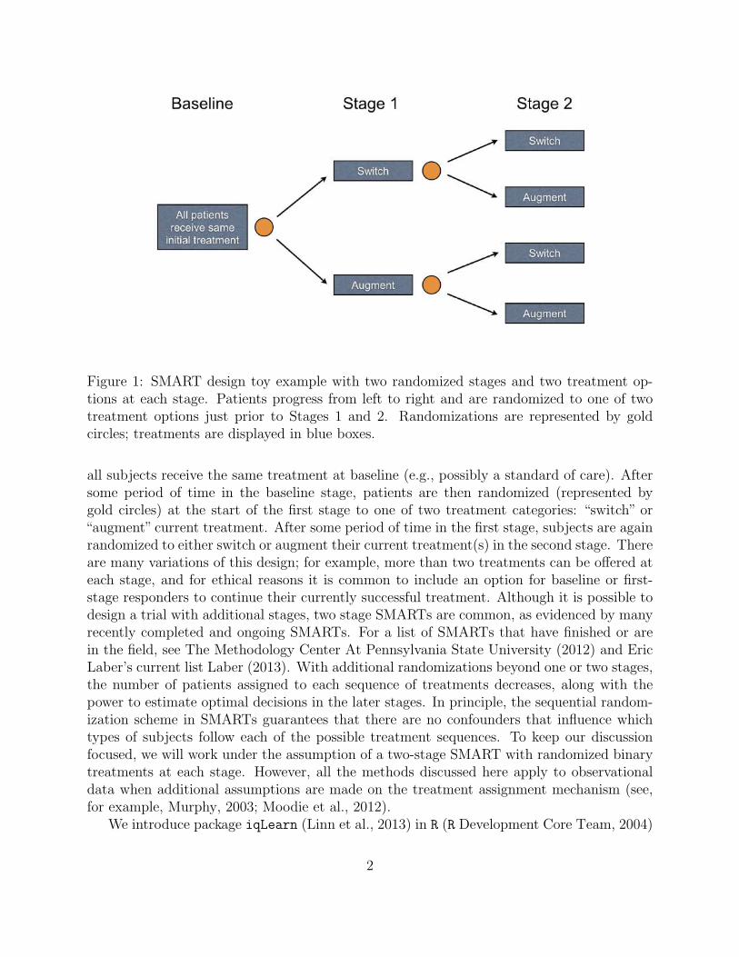
Figure 1: SMART design toy example with two randomized stages and two treatment op-tions at each stage. Patients progress from left to right and are randomized to one of twotreatment options just prior to Stages 1 and 2. Randomizations are represented by goldcircles; treatments are displayed in blue boxes.

all subjects receive the same treatment at baseline (e.g., possibly a standard of care). Aftersome period of time in the baseline stage, patients are then randomized (represented bygold circles) at the start of the first stage to one of two treatment categories: “switch” or“augment” current treatment. After some period of time in the first stage, subjects are againrandomized to either switch or augment their current treatment(s) in the second stage. Thereare many variations of this design; for example, more than two treatments can be offered ateach stage, and for ethical reasons it is common to include an option for baseline or first-stage responders to continue their currently successful treatment. Although it is possible todesign a trial with additional stages, two stage SMARTs are common, as evidenced by manyrecently completed and ongoing SMARTs. For a list of SMARTs that have finished or arein the field, see The Methodology Center At Pennsylvania State University (2012) and EricLaber’s current list Laber (2013). With additional randomizations beyond one or two stages,the number of patients assigned to each sequence of treatments decreases, along with thepower to estimate optimal decisions in the later stages. In principle, the sequential random-ization scheme in SMARTs guarantees that there are no confounders that influence whichtypes of subjects follow each of the possible treatment sequences. To keep our discussionfocused, we will work under the assumption of a two-stage SMART with randomized binarytreatments at each stage. However, all the methods discussed here apply to observationaldata when additional assumptions are made on the treatment assignment mechanism (see,for example, Murphy, 2003; Moodie et al., 2012).

We introduce package iqLearn (Linn et al., 2013) in R (R Development Core Team, 2004)

2

for estimating optimal DTRs from data obtained from a two stage trial with two treatmentsat each stage using Interactive Q-learning (IQ-learning; Laber et al., 2013). Althoughwe recommend using IQ-learing instead of Q-learning in most practical settings based ondevelopments in Section 2 and Laber et al. (2013), a comparison of the regimes estimated bythe two methods may be of interest to some data analysts. Thus, functions for estimationof a regime by the Q-learning algorithm are also included in iqLearn for completeness.Introductions to both Q- and IQ-learning are provided in Section 2. Section 3 provides acase-study illustrating the iqLearn package. A brief discussion of future work concludes thepaper in Section 4.

2 Q-learning and Interactive Q-learning

We assume data are collected from a two-stage randomized trial with binary treatments ateach stage, resulting in n i.i.d. patient trajectories of the form (X1, A1,X2, A2, Y ). The vari-ables in the trajectory are: baseline covariates, X1 ∈ R

p1 ; first-stage randomized treatment,A1 ∈ {−1, 1}; covariates collected during the first-stage but prior to second-stage treatmentassignment, X2 ∈ R

p2 ; second-stage randomized treatment, A2 ∈ {−1, 1}; and the response,Y ∈ R, collected at the conclusion of the trial. We assume Y has been coded so that highervalues indicate more positive clinical outcomes. To simplify notation, we group variablescollected prior to each treatment randomization into a history vector H t, t = 1, 2. That is,H1 = X1 and H2 = (X⊺

1, A1,X⊺2)

⊺.A DTR is a pair of functions π = (π1, π2) where πt maps the domain of H t into the

space of available treatments {−1, 1}. Under π a patient presenting at time t with historyH t = ht is assigned treatment πt(ht). The goal is to estimate a DTR that when applied ina population of patients of interest, the expected outcome is maximized. Define the valueof a fixed regime π as V π , E

π(Y ), where Eπ denotes the expectation when treatment

is assigned according to the policy π. The optimal treatment regime, πopt, maximizes thevalue function:

Eπopt

(Y ) = supπ

EπY.

In the next two sections, we explain how an optimal regime can be estimated from datausing Q-learning and IQ-learning. The IQ-learning estimated optimal decision rules will bedenoted by πIQ−opt

t and the Q-learning analogs by πQ−optt . Both methods are implemented

in the iqLearn package.

2.1 Q-learning

Q-learning (Watkins, 1989; Watkins and Dayan, 1992; Murphy, 2005b) is an approximatedynamic programming algorithm that can be used to estimate an optimal DTR from obser-

3

vational or randomized study data. Define the Q-functions:

Q2(h2, a2) , E(Y |H2 = h2, A2 = a2),

Q1(h1, a1) , E

(max

a2∈{−1,1}Q2(H2, a2)|H1 = h1, A1 = a1

).

The Q-function at stage two measures the Quality of assigning a2 to a patient presentingwith history h2. Similarly, Q1 measures the quality of assigning a1 to a patient with h1,assuming an optimal decision rule will be followed at stage two. Were the Q-functionsknown, dynamic programming (Bellman, 1957) gives the optimal solution, π opt

t (ht) =argmaxat∈{−1,1} Qt(h1, at). Since the underlying distribution of the patient histories is notknown, the conditional expectations that define the Q-functions are unknown and must beapproximated. Q-learning approximates the Q-functions with regression models; commonlylinear models are chosen in practice because they yield simple, interpretable models. Wewill consider linear models of the form: Qt(ht, at; βt) = h

⊺t0βt0 + ath

⊺t1βt1, t = 1, 2, where ht0

and ht1 include an intercept and a subset of variables collected in ht. Define βt , (β⊺t0, β

⊺t1)

⊺.The Q-learning algorithm is given below.

Q-learning Algorithm:

Q1. Modeling: Regress Y on H20,H21, A2 to obtain

Q2(H2, A2; β2) = HT20β20 + A2H

T21β21.

Q2. Maximization: Define Y , maxa2∈{−1,1} Q2(H2, a2, β2).

Y = HT20β20 + |HT

21β21| is the predicted futureoutcome assuming the optimal decision is madeat stage two.

Q3. Modeling: Regress Y on H10,H11, A1 to obtain

Q1(H1, A1; β1) = HT10β10 + A1H

T11β11.

The tth-stage optimal decision rule then assigns the treatment at that maximizes the esti-mated Qt-function,

πQ−optt (ht) = argmax

atQt(ht, at; βt).

In Q-learning with linear models, this can be written as

πQ−optt (ht) = sign(h⊺

t1β21)

The first modeling step in the Q-learning algorithm is a standard multiple regressionproblem to which common model building and model checking techniques can be appliedto find a parsimonious, well-fitting model. The absolute value in the definition of Y ariseswhen A2 is coded as {−1, 1}, since argmaxa2 Q2(H2, a2; β2) = sign(H⊺

21β21). The second

4

modeling step (Q3) requires modeling the conditional expectation of Y . This can be writtenas

Q1(H1, A1) = E(Y |H1, A1)

= E(H⊺20β20 + |H⊺

21β21| | H1, A1). (1)

Due to the absolute value function, Y is a nonsmooth, nonmonotone transformation of H2.Thus, the linear model in step Q3 is generally misspecified. In addition, the nonsmooth,nonmonotone max operator in step Q2 leads to difficult nonregular inference for the param-eters that index the first stage Q-function (Robins, 2004; Chakraborty et al., 2010; Laberet al., 2010; Song et al., 2011; Chakraborty et al., 2013). In the next section, we develop analternative to Q-learning, which we call IQ-learning, that addresses the applied problem ofbuilding good models for the first-stage Q-function and avoids model misspecification for alarge class of generative models.

2.2 Interactive Q-learning (IQ-learning)

IQ-learning differs from Q-learning in the order in which maximization step (Q2 in theQ-learning algorithm) is performed. We demonstrate how the maximization step can be de-layed, enabling all modeling to be performed before this nonsmooth, nonmonotone transfor-mation. This reordering of modeling and maximization steps facilitates the use of standard,interactive model building techniques because all terms to be modeled are linear, and hencesmooth and monotone, transformations of the data. For a large class of generative models,IQ-learning more accurately estimates the first-stageQ-function, resulting in a higher-qualityestimated decision rule (Laber et al., 2013). Another advantage of IQ-learning is that inmany cases, conditional mean and variance modeling techniques (Carroll and Ruppert, 1988)offer a nice framework for the necessary modeling steps. These mean and variance models areinterpretable, and the coefficients indexing them enjoy normal limit theory. Thus, they arebetter suited to inform clinical practice than the misspecified first-stage model in Q-learningwhose indexing parameters are nonregular. However, the mean-variance modeling approachwe advocate here is not necessary and other modeling techniques may be applied as needed.Indeed, a major advantage and motivation for IQ-learning is the ability for the seasonedapplied statistician to build high-quality models using standard interactive techniques formodel diagnosis and validation.

IQ- and Q-learning do not differ at step one (Q1), which we refer to as the second-stage

regression. Define m(H2; β2) , H⊺20β20, and ∆(H2; β2) , H

⊺21β21. We call the first term the

main effect function and the second the contrast function. ∆(H2; β2) “contrasts” the qualityof the second-stage treatments: ∆(H2; β2) = 1

2{Q2(H2, A2 = 1) − Q2(H2, A2 = −1)}. In

the IQ-learning framework, the first-stage Q-function is defined as

Q1(h1, a1) , E(m(H2; β2)|H1 = h1, A1 = a1) +

∫|z|g(z | h1, a1)dz, (2)

where g(· | h1, a1) is the conditional distribution of the contrast function ∆(H2; β2) givenH1 = h1 and A1 = a1. In fact, (2) is equivalent to the representation of Q1 in (1), only

5

the conditional expectation has been split into two separate expectations and the second hasbeen written in integral form. Instead of modeling the conditional expectation in (1) directly,IQ-learning separately models E(m(H2; β2)|H1 = h1, A1 = a1) and g(· | h1, a1). AlthoughIQ-learning trades one modeling step (Q3) for two, splitting up the conditional expectationin (1) is advantageous because the terms that require modeling are now smooth, monotonefunctionals of the data. The maximization occurs when the integral in (2) is computed,which occurs after the conditional density g(· | h1, a1) has been estimated. The IQ-learningalgorithm is given below.

6

IQ-learning Algorithm:

IQ1. Modeling: Regress Y on H20,H21, A2 to obtain

QIQ2 (H2, A2; β2) = H

T20β20 + A2H

T21β21.

IQ2. Modeling: Regress HT20β20 on H1, A1 to obtain an esti-

mator ℓ(H1, A1) of E(HT20β20|H1, A1).

IQ3. Modeling: Use {(HT21,iβ21,H1,i, A1,i)}

ni=1 to obtain an es-

timator g(· | H1, A1) of g(· | H1, A1).

IQ4. Maximization: Combine the above estimators to form

QIQ1 (H1, A1) = ℓ(H1, A1) +

∫|z|g(z |

H1, A1)dz.

The IQ-learning estimated optimal DTR assigns the treatment at stage t as the maximizerof the estimated stage-t Q-function πIQ−opt

t (ht) = argmaxat QIQt (ht, at; βt).

We note that it is possible to obtain QIQ1 in IQ4 by modeling the bivariate conditional

distribution of m(H2; β2) and ∆(H2; β2) given H1 and A1 instead of separate modelingsteps IQ2 and IQ3. However, it is often easier to assess model fits using standard residualdiagnostics and other well-established model checking tools when E(H⊤

20β20 | H1, A1) andg(· | H1, A1) are modeled separately.

2.3 Remark about density estimation in IQ3

Step IQ3 in the IQ-learning algorithm requires estimating a one-dimensional conditional den-sity. In Laber et al. (2013) we accomplish this using mean-variance, location-scale estimatorsof g(· | h1, a1) of the form

g(z | h1, a1) =1

σ(h1, a1)φ

(z − µ(h1, a1)

σ(h1, a1)

),

where µ(h1, a1) is an estimator of µ(h1, a1) , E {∆(H2; β2) | H1 = h1, A1 = a1}, σ2(h1, a1)

is an estimator of σ2(h1, a1) , E {(∆(H2; β2)− µ(h1, a1))2 | H1 = h1, A1 = a1}, and φ is

an estimator of the density of the standardized residuals {∆(H2; β2)− µ(h1, a1)} /σ(h1, a1),say φh1,a1 , which we assume does not depend on the history h1 or the treatment a1. Mean-variance function modeling tools are well-studied and applicable in many settings (Carrolland Ruppert, 1988). Currently, iqLearn implements mean-variance modeling steps to esti-mate g(· | h1, a1) with the option of using a standard normal density or empirical distribution

estimator for φ.

7

gender ∈ {0, 1} : patient gender, coded female (0) and male (1).race ∈ {0, 1} : patient race, coded African American (0) or other (1).parent_BMI ∈ R : parent BMI measured at baseline.baseline_BMI ∈ R : patient BMI measured at baseline.A1 ∈ {−1, 1} : first-stage randomized treatment, coded so that A1 = 1 cor-

responds to meal replacement (MR) and A1 = -1 correspondsto conventional diet (CD).

month4_BMI ∈ R : patient BMI measured at month 4.A2 ∈ {−1, 1} : second-stage randomized treatment, coded so that A2 = 1 cor-

responds to meal replacement (MR) and A2 = -1 correspondsto conventional diet (CD).

month12_BMI ∈ R : patient BMI measured at month 12.

Table 1: Description of variables in bmiData.

3 Using the iqLearn Package

3.1 Preparing dataset bmiData

The examples in this section will be illustrated using a simulated dataset called bmiData

which is included in the iqLearn package. The data are generated to mimic a two-stageSMART of body mass index (BMI) reduction with two treatments at each stage. Thevariables, treatments, and outcomes in bmiData were based on a small subset of variablescollected in a clinical trial studying the effect of meal replacements (MRs) on weight loss andBMI reduction in obese adolescents; see Berkowitz et al. (2010) for a complete description ofthe original randomized trial. Descriptions of the generated variables in bmiData are givenin Table (1). Baseline covariates include gender, race, parent_BMI, and baseline_BMI.Four- and twelve-month patient BMI measurements were also included to reflect the originaltrial design. In the generated data, treatment was randomized to meal replacement (MR)or conventional diet (CD) at both stages, each with probability 0.5. In the original study,patients randomized to CD in stage one remained on CD with probability one in stage two.Thus, our generated data arises from a slightly difference design than that of the originaltrial. In addition, some patients in the original data set were missing the final twelve monthresponse as well as various first- and second-stage covariates. Our generated data is complete,and the illustration of IQ- and Q-learning with iqLearn that follows is presented under theassumption that missing data have been addressed prior to using these methods (for example,using an appropriate imputation strategy).

After installing iqLearn, load the package:

> library (iqLearn)

Next, load bmiData into the workspace with

> data (bmiData)

8

The generated dataset bmiData is a data frame with 210 rows corresponding to patientsand 8 columns corresponding to covariates, BMI measurements, and assigned treatments.

> dim (bmiData)

[1] 210 8

> head (bmiData)

gender race parent_BMI baseline_BMI month4_BMI month12_BMI A1 A2

1 0 1 31.59683 35.84005 34.22717 34.27263 CD MR

2 1 0 30.17564 37.30396 36.38014 36.38401 CD MR

3 1 0 30.27918 36.83889 34.42168 34.41447 MR CD

4 1 0 27.49256 36.70679 32.52011 32.52397 CD CD

5 1 1 26.42350 34.84207 33.72922 33.73546 CD CD

6 0 0 29.30970 36.68640 32.06622 32.15977 MR MR

Recode treatments Meal Replacement (MR) and Conventional Diet (CD) as 1 and -1, re-spectively.

> bmiData$A1[which (bmiData$A1=="MR")] = 1

> bmiData$A1[which (bmiData$A1=="CD")] = -1

> bmiData$A2[which (bmiData$A2=="MR")] = 1

> bmiData$A2[which (bmiData$A2=="CD")] = -1

> bmiData$A1 = as.numeric (bmiData$A1)

> bmiData$A2 = as.numeric (bmiData$A2)

We use the negative percent change in BMI at month 12 from baseline as our final outcome:

> y = -100*(bmiData$month12_BMI -

+ bmiData$baseline_BMI)/bmiData$baseline_BMI

Thus, higher values indicate greater BMI loss, a desirable clinical outcome. We will nextshow how to implement IQ-learning with the iqLearn package to obtain an estimate of theoptimal DTR, πIQ−opt = (πIQ−opt

1 , πIQ−opt2 ), that maximizes the expected BMI reduction.

3.2 IQ-learning functions

The current version of the iqLearn package only allows specification of linear models at allmodeling steps. An advantage of IQ-learning over Q-learning is that for a large class ofgenerative models, linear models are correctly specified at each modeling step (Laber et al.,2013). In general, this is not true for Q-learing at the first-stage. In our illustrations, we skipsome of the typical exploratory techniques that a careful analyst would employ to find thebest-fitting models. These steps would not be meaningful with the bmiData dataset sinceit was simulated with linear working models and would only detract from our main focus

9

which is to present the steps of the IQ-learning algorithm using the functions in iqLearn.Analysts who use IQ-learning should employ standard data exploration techniques betweeneach modeling step. Another consequence of using generated data is that we will not intrepretany coefficients or comment on model fit. In fact, most of the R2 statistics are nearly 1 andmany terms appear highly significant, reflecting the fact that the data are not real. Allmodels and decision rules estimated in this section are strictly illustrative. In addition, theresults in this section are not representative of the results of the original meal replacementstudy.

STEP IQ1: second-stage regression

The first step in the IQ-learning algorithm is to model the response as a function ofsecond-stage history variables and treatment. We model the second-stage Q-function as alinear function of gender, parent_BMI, month4_BMI, and A2, fitting the model using leastsquares.

> fitIQ2 = learnIQ2 (y ~ gender + parent_BMI + month4_BMI +

+ A2*(parent_BMI + month4_BMI), data=bmiData, treatName="A2",

+ intNames=c ("parent_BMI", "month4_BMI"))

The function learnIQ2() creates an object of type learnIQ2 that contains a lm() objectof the linear regression in addition to several other components. We have implemented theformula specification above. The user can specify any formula admissible by lm(), but itmust include the main effect of treatment A2 and at least one treatment interaction term.The second and third arguments specify which variable codes the second stage treatment andcovariates interacting with treatment respectively. If exploratory work suggests there are notreatment-by-covariate interactions at the second stage, IQ-learning has no advantage overQ-learning, and it would be appropriate to model the conditional expectation of Y directlyat the first stage. The default S3 method for learnIQ2() requires a matrix or data frame ofvariables to use as main effects in the linear model. Below, we create this data frame.

> s2vars = bmiData[, c(1,3,5)]

> head (s2vars)

gender parent_BMI month4_BMI

1 0 31.59683 34.22717

2 1 30.17564 36.38014

3 1 30.27918 34.42168

4 1 27.49256 32.52011

5 1 26.42350 33.72922

6 0 29.30970 32.06622

The default method also requires a vector of indices that point to the columns of s2varsthat should be included as treatment interactions in the model.

> s2ints = c (2,3)

10

The default method for learnIQ2() is

> fitIQ2 = learnIQ2 (H2=s2vars, Y=y, A2=bmiData$A2, s2ints=s2ints)

To print the regression output we can call a summary() of the learnIQ2 object.

> summary (fitIQ2)

Stage 2 Regression:

Call:

lm(formula = Y ~ s2. - 1)

Residuals:

Min 1Q Median 3Q Max

-20.5929 -3.7614 -0.1526 4.4436 17.4479

Coefficients:

Estimate Std. Error t value Pr(>|t|)

s2.intercept 41.28845 3.98789 10.353 < 2e-16 ***

s2.gender -0.64891 0.89924 -0.722 0.4714

s2.parent_BMI -0.15509 0.10236 -1.515 0.1313

s2.month4_BMI -0.82067 0.13992 -5.865 1.8e-08 ***

s2.A2 -7.38709 3.97545 -1.858 0.0646 .

s2.parent_BMI:A2 0.20223 0.10201 1.983 0.0488 *

s2.month4_BMI:A2 0.02816 0.13982 0.201 0.8406

---

Signif. codes: 0 ‘***’ 0.001 ‘**’ 0.01 ‘*’ 0.05 ‘.’ 0.1 ‘ ’ 1

Residual standard error: 6.437 on 203 degrees of freedom

Multiple R-squared: 0.605, Adjusted R-squared: 0.5914

F-statistic: 44.42 on 7 and 203 DF, p-value: < 2.2e-16

The plot() function can be used to obtain residual diagnostic plots from the linear regres-sion, shown in Figure 2. These plots can be used to check the usual normality and constantvariance assumptions. The learnIQ2 object returns a list that contains the estimated maineffect coefficients,

> fitIQ2$betaHat20

s2.intercept s2.gender s2.parent_BMI s2.month4_BMI

41.2884512 -0.6489144 -0.1550899 -0.8206701

and interaction coefficients,

11

−5 0 5 10 15

−20

010

20

Fitted values

Res

idua

ls

●●●

●

●

●

●●

● ●●

●

●

●

●

●●

●

●

●

●●

● ●

●●●

●

● ●●

●●●●●

●

●

●

●

●●

● ●●●

●●●●

●

● ●

●●

●●

●

●●●

●

●●

●● ●

●

●

●

●

● ●

●

● ●●●● ●

●

●

●

●

●

●●

● ●

●

●

●

●

●●

●●

●●

●●

●●●●

●

●● ●

●

●●

●

●

●

●

●

●●

●

●

●

●

●

●●

●

●●

●

●●

●

●●

●

●

●

●●

●

●

●

●●

●● ●●

●

●

●

●

●●

●●●

●

●

●

●

●

●●

●

●

●●

●●

●

●

●

●● ●●

●●●

●

●

●

●

●●

●

●

●

●●

●

●

●

●

●

●

●

● ●

●

●●

●

●

●

●●

●

Residuals vs Fitted

197

184143

●●●

●

●

●

●●

●●

●●

●

●

●

●●

●

●

●

●●

●●

●●●

●

●●●

●●●●●

●

●

●

●

●●

●●●●

●●●●

●

●●

●●

●●

●

●●●

●

●●

●●●

●

●

●

●

●●

●

●●●

●●●

●

●

●

●

●

●●

●●

●

●

●

●

●●

●●

●●

●

●

●●●●

●

● ●●

●

●●

●

●

●

●

●

●●

●

●

●

●

●

●●

●

●●

●

● ●

●

●●

●

●

●

●●

●

●

●

●●

●●●●

●

●

●

●

●●

●●●

●

●

●

●

●

●●

●

●

●●

●●

●

●

●

●●●●

●●●

●

●

●

●

●

●

●

●

●

●●

●

●

●

●

●

●●

●●

●

●●

●

●

●

●●

●

−3 −2 −1 0 1 2 3

−3

−1

12

3

Theoretical Quantiles

Sta

ndar

dize

d re

sidu

als

Normal Q−Q

197

184143

−5 0 5 10 15

0.0

0.5

1.0

1.5

Fitted values

Sta

ndar

dize

d re

sidu

als

●●

●●

●

●

●●

●●

●

●

●

● ●

●

●

●

●

●

●

●

●

●

●●

●

●

●●

●

●●

●●●

●

●

●

●

●●

● ●●●

●●

●●

●

●●

●●

●●

●

●●

●

●

●

●

●●

●

●

●

●

●

●●

●

● ●

●

●

●●

●

●

●

●

●

●

●●●

●

●

●

●●

●

●

●

●

●

●

●●●

●●

●

●

●●

●

●

●

●●

●

●

●●

●

●

●

●

●

●

●●

●

●●

●

●●

●

●

●

●

●

●

●●

●

●

●

●●●

●●

●

●

●

●

●

●

●

●●●

●

●

●

●

●

●●

●

●

●●

●

●

●

●

●●

● ●●

●●

●

●

●

●

●

●

●

●

●

●

●●

●

●

●

●

●

●

●

●

●

●

●

●●

●

●

●

●

●

Scale−Location197

184143

0.00 0.05 0.10 0.15

−4

−2

01

23

Leverage

Sta

ndar

dize

d re

sidu

als

● ●●

●

●

●

●●

● ●●

●

●

●

●

●●

●

●

●

●●

●●

● ●●

●

●●●

●●●●●

●

●

●

●

●●

●●●●

● ●●●

●

●●

●●

●●

●

●●●

●

●●

●●●

●

●

●

●

● ●

●

●●●

●●●

●

●

●

●

●

●●

●●

●

●

●

●

●●

●●

●●

●●

●●●●

●

● ●●

●

●●

●

●

●

●

●

●●

●

●

●

●

●

●●

●

●●

●

● ●

●

●●

●

●

●

● ●

●

●

●

● ●

●● ●●

●

●

●

●

●●

●●●

●

●

●

●

●

●●

●

●

●●

●●

●

●

●

●● ●●

● ●●

●

●

●

●

●●

●

●

●

● ●

●

●

●

●

●

●●

●●

●

●●

●

●

●

●●

●

Cook's distance

Residuals vs Leverage

138

143

121

Figure 2: Residual diagnostic plots from the second-stage regression in IQ-learning.

> fitIQ2$betaHat21

s2.A2 s2.parent_BMI:A2 s2.month4_BMI:A2

-7.38708909 0.20223376 0.02815973

The first term of $betaHat20 is the intercept and the first term of $betaHat21 is the maineffect of treatment A2. Other useful elements in the list include the vector of estimatedoptimal second-stage treatments for each patient in the dataset ($optA2), the lm() object($s2Fit), the vector of estimated main effect terms ($main), and the vector of estimatedcontrast function terms ($contrast).

STEP IQ2: main effect function regression

12

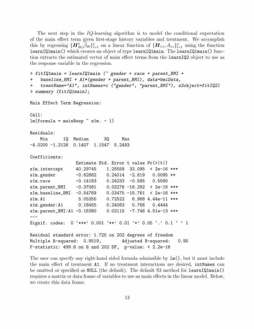
The next step in the IQ-learning algorithm is to model the conditional expectationof the main effect term given first-stage history variables and treatment. We accomplishthis by regressing {H⊺

20,iβ20}ni=1 on a linear function of {H1,i, A1,i}

ni=1 using the function

learnIQ1main() which creates an object of type learnIQ1main. The learnIQ1main() func-tion extracts the estimated vector of main effect terms from the learnIQ2 object to use asthe response variable in the regression.

> fitIQ1main = learnIQ1main (~ gender + race + parent_BMI +

+ baseline_BMI + A1*(gender + parent_BMI), data=bmiData,

+ treatName="A1", intNames=c ("gender", "parent_BMI"), s2object=fitIQ2)

> summary (fitIQ1main);

Main Effect Term Regression:

Call:

lm(formula = mainResp ~ s1m. - 1)

Residuals:


-4.0200 -1.2126 0.1407 1.1547 5.2493

Coefficients:


s1m.intercept 40.29745 1.25558 32.095 < 2e-16 ***

s1m.gender -0.62882 0.24014 -2.619 0.0095 **

s1m.race -0.14183 0.24233 -0.585 0.5590

s1m.parent_BMI -0.37081 0.02276 -16.292 < 2e-16 ***

s1m.baseline_BMI -0.54769 0.03475 -15.761 < 2e-16 ***

s1m.A1 5.05355 0.72522 6.968 4.44e-11 ***

s1m.gender:A1 0.18455 0.24083 0.766 0.4444

s1m.parent_BMI:A1 -0.16380 0.02115 -7.746 4.51e-13 ***

---

Signif. codes: 0 ‘***’ 0.001 ‘**’ 0.01 ‘*’ 0.05 ‘.’ 0.1 ‘ ’ 1




The user can specify any right-hand sided formula admissible by lm(), but it must includethe main effect of treatment A1. If no treatment interactions are desired, intNames canbe omitted or specified as NULL (the default). The default S3 method for learnIQ1main()requires a matrix or data frame of variables to use as main effects in the linear model. Below,we create this data frame.

13

> s1vars = bmiData[, 1:4]

> head (s1vars)

gender race parent_BMI baseline_BMI

1 0 1 31.59683 35.84005

2 1 0 30.17564 37.30396

3 1 0 30.27918 36.83889

4 1 0 27.49256 36.70679

5 1 1 26.42350 34.84207

6 0 0 29.30970 36.68640

The default method also requires a vector of indices that point to the columns of s1vars thatshould be included as treatment interactions in the model. If no interactions are desired,s1mainInts can be omitted, as the default is NULL.

> s1mainInts = c (1,3)

The default method for learnIQ1main() is

> fitIQ1main = learnIQ1main (object=fitIQ2, H1Main=s1vars,

+ A1=bmiData$A1, s1mainInts=s1mainInts)

where the first argument is the learnIQ2 object. Again, plot() gives residual diagnosticplots from the fitted regression model, shown in Figure 3. Elements of the list returned bylearnIQ1main() include the estimated main effect coefficients,

14

0 5 10

−4

02

46

Fitted values

Res

idua

ls

●

●●

●

●

●●

●

●

●

●●

●

● ●

●

●

●

●

●

●●

●

●●

●●

● ●

●●

●●●

●

●

●●

●

●

●

●

●●●

●●

●

●●

●

●

●

●

●

●

●

●

●

●

●

●

●

●

●

●

●

●

●

●

●●

●

●

●

●●

●●●

●●

●

●

●

●

●

●●

●

●

●

●

● ●●●

●

●

●

●

●●

● ●

●●

●●

●

●●

●

●

●

●

●

●

●

●

●

●●

●

●●

●●●

●●

●

●

●

●●

●●

●

●

●

●

●

●

●

●●

●

●●

●●

●

●●

●

●

●●

●

●

●●

● ●●

●

●

●●

●

●

●

●

● ●

●●●

●

●

●

●

●

●

●●

●

●

●

●

●

●

●

●

●●

●●

●●

● ●● ●

●

●

●

●

●

Residuals vs Fitted

184156148

●

●

●

●

●

●●

●

●

●

●●

●

●●

●

●

●

●

●

●

●

●

● ●

●●

●●

●●

●●

●

●

●

●●

●

●

●

●

●●●

●●

●

●●

●

●

●

●

●

●

●

●

●

●

●

●

●

●

●

●

●

●

●

●

●●

●

●

●

●●

●●

●

●

●

●

●

●

●

●

●●

●

●

●

●

●●●●

●

●

●

●

●●

●●

●●

●●

●

●●

●

●

●

●

●

●

●

●

●

●●

●

●●

●●●

●●

●

●

●

●●

●●

●

●

●

●

●

●

●

●●

●

●●

●●

●

●●

●

●

●●

●

●

●●

●●●

●

●

●●

●

●

●

●

●●

●●●

●

●

●

●

●

●

●●

●

●

●

●

●

●

●

●

●●

●●

●●

●●●●

●

●

●

●

●

−3 −2 −1 0 1 2 3

−2

01

23


Sta

ndar

dize

d re

sidu

als

Normal Q−Q

184

148156

0 5 10

0.0

0.5

1.0

1.5

Fitted values

Sta

ndar

dize

d re

sidu

als

●

●

●●

●●

●

●

●

●

●

●

●

● ●●

●

●

●

●

●

●

●

●

●

●

●

●

●●

●

●

●

●

●

●

●

●

●

●

●

●

●●

●

●

●

●

●●

●●

●

●

●

●

●

●

●

●

●

●

●

●●

●

●

●

●

●

●●

●

●●

●

●

●●●

●

●

●

●

●

●

●

●

●

●

●

●

●

● ●

●●●

●

●

●

●

●

●

●

●●

●

●●

●●

●

●

●

●

●

●

●

●

●

●●

●

●●

●

●

●

●

●

●

●

●

●

●

●

●

●

●

●

●

●●

●

●●

●

●●

●

●

●

●●

●

●

●

●

●

●

●

●

●●

●

●

●

●

●●

●●

●

●●

●●●

●

●

●

●

●

●

●

●

●

●

●

●

● ●

●

● ●●

●●

●

●

●●

●

●

●

●

●

●

●

Scale−Location184

148156

0.00 0.04 0.08 0.12

−3

−1

12

3

Leverage

Sta

ndar

dize

d re

sidu

als

●

●●

●

●

●●

●

●

●

●●

●

● ●

●

●

●

●

●

●●

●

●●

●●●●

●●

●●●

●●

●●

●

●

●

●

● ●●

●●

●

●●

●

●

●

●

●

●

●

●

●

●

●

●

●

●

●

●

●

●

●

●

●●

●

●

●

●●

●●●

●●

●

●

●

●

●

●●

●

●

●

●

●●●●

●

●

●

●

●●●●

●●

●●

●

●●

●

●

●

●

●

●

●

●

●

● ●

●

● ●

●● ●

●●

●

●

●

●●

●●

●

●

●

●

●

●

●

●●

●

●●

●●

●

● ●

●

●

●●

●

●

● ●

●●●

●

●

●●

●

●

●

●

●●

●●●

●

●

●

●

●

●

●●

●

●

●

●

●

●

●

●

●●

●●

●●

●●●●

●

●

●

●

●

Cook's distance


184148

142

Figure 3: Residual diagnostic plots from the regression model for the main effect term.

> fitIQ1main$alphaHat0

s1m.intercept s1m.gender s1m.race s1m.parent_BMI

40.2974492 -0.6288155 -0.1418311 -0.3708085

s1m.baseline_BMI

-0.5476887

and estimated interaction coefficients,

> fitIQ1main$alphaHat1

s1m.A1 s1m.gender:A1 s1m.parent_BMI:A1

5.0535529 0.1845549 -0.1637973

15

Other elements are used in future steps of the algorithm.

STEP IQ3: contrast function density modeling

The final modeling step in IQ-learning is to model the conditional density of the contrastfunction given first-stage history variables and treatment. We will accomplish this by con-sidering the class of location-scale density models and employing standard conditional meanand variance modeling techniques. Thus, we begin by modeling the conditional mean of thecontrast function using learnIQ1cm().

> fitIQ1cm = learnIQ1cm (~ gender + race + parent_BMI +

+ baseline_BMI + A1*(gender + parent_BMI + baseline_BMI),

+ data=bmiData, treatName="A1", intNames=c ("gender", "parent_BMI",

+ "baseline_BMI"),

+ s2object=fitIQ2);

> summary (fitIQ1cm)

Contrast Mean Regression:

Call:

lm(formula = cmResp ~ s1cm. - 1)

Residuals:


-0.140304 -0.040954 -0.002024 0.038278 0.140948

Coefficients:


s1cm.intercept -7.3287896 0.0425272 -172.332 < 2e-16 ***

s1cm.gender -0.0044590 0.0080960 -0.551 0.582407

s1cm.race 0.0072002 0.0081239 0.886 0.376517

s1cm.parent_BMI 0.2094135 0.0007631 274.428 < 2e-16 ***

s1cm.baseline_BMI 0.0183059 0.0011694 15.654 < 2e-16 ***

s1cm.A1 -0.0520737 0.0425007 -1.225 0.221918

s1cm.gender:A1 -0.0090028 0.0080828 -1.114 0.266683

s1cm.parent_BMI:A1 0.0066622 0.0007675 8.681 1.35e-15 ***

s1cm.baseline_BMI:A1 -0.0040765 0.0011732 -3.475 0.000626 ***

---

Signif. codes: 0 ‘***’ 0.001 ‘**’ 0.01 ‘*’ 0.05 ‘.’ 0.1 ‘ ’ 1



F-statistic: 1.183e+04 on 9 and 201 DF, p-value: < 2.2e-16

16

The user can specify any right-hand sided formula admissible by lm(), but it must includethe main effect of treatment A1. The default S3 method for learnIQ1cm() requires a matrixor data frame of variables to use as main effects in the linear model and indicies indicating thetreatment interaction effects. intNames can be omitted or specified as NULL if no interactionsare desired. We will use s1vars and specify the interactions with a vector for s1cmInts.

> s1cmInts = c (1,3,4)

The default method is

> fitIQ1cm = learnIQ1cm (object=fitIQ2, H1CMean=s1vars, A1=bmiData$A1,

+ s1cmInts=s1cmInts);

Figure (4) displays the residual diagnostics produced by plot(). The learnIQ1cm() functionreturns a list with several elements. The residuals from the contrast mean fit are stored in$cmeanResids. Estimated main effect coefficients can be accessed,

> fitIQ1cm$betaHat10

s1cm.intercept s1cm.gender s1cm.race

-7.328789639 -0.004459014 0.007200203

s1cm.parent_BMI s1cm.baseline_BMI

0.209413508 0.018305862

as well as the interaction coefficients,

> fitIQ1cm$betaHat11

s1cm.A1 s1cm.gender:A1 s1cm.parent_BMI:A1

-0.052073685 -0.009002806 0.006662162

s1cm.baseline_BMI:A1

-0.004076464

Other items in the list are used in upcoming steps of the algorithm.After fitting the model for the conditional mean of the contrast function, we must specify

a model for the variance of the residuals. Standard approaches can be used to determine ifa constant variance fit is sufficient. If so,

> fitIQ1var = learnIQ1var (fitIQ1cm)

is the default for estimating the common standard deviation. Equivalently, method=‘homo’can be specified to indicate homoskedastic variance,

> fitIQ1var = learnIQ1var (object=fitIQ1cm, method="homo")

17

−1 0 1 2 3 4

−0.

150.

000.

10

Fitted values

Res

idua

ls

●

●

●

●

●

●●

●

●

●

●●

●

●●

●

●

●

●

●

●

●●

●●

●● ●●

●● ●

●●

●●

●●

●

●

●

●

●●●

●●

●

●●

●

●

●

●

●

●

●

●

●

●

●

●●

●

●

●

●

●

●

●

●●

●●

●

●●

●●●

●

●

●

●

●

●

●

●●

●

●

●

●

●● ●

●

●

●

●

●

●●●

●

●●

●

●

●

●●●

●●

●

●

●●

●

●

●

●

●

●●

●

●●

●●●

●

●

●●

●●

●

●

●

●

●●

●

●●

●

●●

●●

●

● ●

●

● ●

●

●

●

●

●

●●

●

●

●

●●

●

●

●

●

●●

●

●●

●

●

●

●

●

●

●

●

●

●

●

●

●

●

●

●

●

●

●●

●● ●

●●

●

●

●

●

●

●

Residuals vs Fitted

20

184156

●

●

●

●

●

●●

●

●

●

●●

●

●

●

●

●

●

●

●

●

●●

●●

●●●●

●●●●

●

●

●

●●

●

●

●

●

●●

●

●●

●

●●

●

●

●

●

●

●

●

●

●

●

●

●●

●

●

●

●

●

●

●

●●

●

●

●

●●

●●

●

●

●

●

●

●

●

●

●●

●

●

●

●

●●●

●

●

●

●

●

●●●

●

●●

●

●

●

●●●

●●

●

●

●●

●

●

●

●

●

●●

●

●●

●●●

●

●

●●

●●

●

●

●

●

●●

●

●●

●

●●

●●

●

●●

●

●●

●

●

●

●

●

●●

●

●

●

●●

●

●

●

●

●●

●

●●

●

●

●

●

●

●

●

●

●

●

●

●

●

●

●

●

●

●

●●

●●●

●

●●

●

●

●

●

●

−3 −2 −1 0 1 2 3

−2

01

23


Sta

ndar

dize

d re

sidu

als

Normal Q−Q

184

20

156

−1 0 1 2 3 4

0.0

0.5

1.0

1.5

Fitted values

Sta

ndar

dize

d re

sidu

als

●

●

●●● ●

●

●

●

●

●●

●

●

●

●

●

●

●

●

●

●

●

●

●

●

●●● ●

●●

●

●

●

●

●●

●

● ●

●

●●

●

●

●

●

●●

● ●

●

●

●

●

●

●

●

●

●

●

●

●●

●

●

●

●

●

●

●

●

● ●

●

●

●●

●●

●

●

●

●●

●

●

●

●

●

●

●

●● ●

●

●

●

●

●

●

●●●

●

●

●

●

●

●

●●

●

●

●

●

●●

●

●●

●

●●●

●

●

●

●●

●

●

●

●

●

●

●

●

●

●

●

●

●

●

●

●

●

●●●

●

●

● ●

●

● ●

●

●●

●

●

●●

●

●

●

●

●●

●●

●

●●

●

●

●

●

●

●

●

●

●

●

●

●

●●

●

●

●

●

●

●

●

●●

●

●●

●

●

●

●

●

●

●

●

Scale−Location18420156

0.00 0.05 0.10 0.15 0.20

−3

−1

12

3

Leverage

Sta

ndar

dize

d re

sidu

als

●

●

●

●

●

●●

●

●

●

●●

●

●●

●

●

●

●

●

●

●●

●●

●●●●

●●●

●●

●●

●●

●

●

●

●

● ●●

●●●

●●

●

●

●

●

●

●

●

●

●

●

●

●●

●

●

●

●

●

●

●

●●

●●

●

●●

●●●

●

●

●

●

●

●

●

●●

●

●

●

●

●●●

●

●

●

●

●

●●●

●

●●

●

●

●

●●●

●●

●

●

●●

●

●

●

●

●

● ●

●

●●

●●●

●

●

●●

●●

●

●

●

●

●●

●

●●

●

●●

●●

●

● ●

●

●●

●

●

●

●

●

●●

●

●

●

●●

●

●

●

●

●●

●

●●

●

●

●

●

●

●

●

●

●

●

●

●

●

●

●

●

●

●

●●

●●●

●●

●

●

●

●

●

●

Cook's distance


184

145

148

Figure 4: Residual diagnostic plots from the linear regression model for the contrast functionmean.

but this additional statement is unnecessary since it is the default. A list is returned withthe estimated common standard deviation of the contrast mean fit residuals ($stdDev), thevector of standardized residuals for each patient in the dataset ($stdResids), and severalother elements, some of which are NULL when method=‘homo’.

If the variance is thought to be non-constant across historiesH1 and/or treatment A1, theoption method=‘hetero’ allows specification of a log-linear model for the squared residuals.As before, the formula should be only right-hand sided and must include the main effectof treatment A1. The default for s1varInts is NULL, which can be used if no interactionsare desired in the model. The formula version and alternate default specification are shownbelow and are similar to previous steps.

> fitIQ1var = learnIQ1var (~ gender + race + parent_BMI +

18

+ baseline_BMI + A1*(parent_BMI), data=bmiData, treatName="A1",

+ intNames=c ("parent_BMI"), method="hetero", cmObject=fitIQ1cm)

> s1varInts = c (3, 4)

> fitIQ1var = learnIQ1var (object=fitIQ1cm, H1CVar=s1vars,

+ s1sInts=s1varInts, method="hetero")

> summary (fitIQ1var)

Variance Model:

Call:

lm(formula = lRes2 ~ s1v. - 1)

Residuals:


-8.5694 -0.8962 0.4247 1.4247 2.9195

Coefficients:


s1v.intercept -8.241606 1.484122 -5.553 8.77e-08 ***

s1v.gender 0.077415 0.285104 0.272 0.7863

s1v.race 0.075925 0.286549 0.265 0.7913

s1v.parent_BMI -0.002661 0.026917 -0.099 0.9213

s1v.baseline_BMI 0.036738 0.040900 0.898 0.3701

s1v.A1 1.921779 1.478243 1.300 0.1951

s1v.parent_BMI:A1 -0.053469 0.027035 -1.978 0.0493 *

s1v.baseline_BMI:A1 -0.002528 0.041195 -0.061 0.9511

---

Signif. codes: 0 ‘***’ 0.001 ‘**’ 0.01 ‘*’ 0.05 ‘.’ 0.1 ‘ ’ 1




Figure (5) displays the residual diagnostics produced by plot(). The learnIQ1var objectreturns a list that includes estimated main effect coefficients,

> fitIQ1var$gammaHat0

s1v.intercept s1v.gender s1v.race s1v.parent_BMI

-7.138610546 0.077414538 0.075925188 -0.002661492

s1v.baseline_BMI

0.036738083

and interaction coefficients,

19

−7.5 −7.0 −6.5 −6.0

−10

−6

−2

24

Fitted values

Res

idua

ls ●

●

●●●

●

●

●

●

●

●● ●

●●

●

●

●

●

●

●

●

●

●

●

●

●●●●

●●

●

●

●●●●

●

●●

●

●●

●

●●●

●

●

● ●

●

●

●

●●

●●

●

●

●●

●●

●

●

●

●

●

●

●

● ●●

●

● ●●●●

●

●●

●●

●

●●

●

●

●

●●

●●●

●

●

●

●

●

●

● ●

●

●

●

●●

●

●●

●

●

●

●●●

●

●

●

●

●● ●

●

●

●

●●

●

●

●

● ●

●

●

●

●

●

●

●

●

●

●

●

●

● ●●●

●

●●

●

● ●

●

● ●

●

●

●●

●

●

●

●

● ●

●●

●

●●

●

●

●

●

●

●

●

●

●

●●

●●

●

●

●●

●

● ●

●

● ●

●● ●

●

●

●

●

●

●

●

●

Residuals vs Fitted

208129

72

●

●

●●●

●

●

●

●

●

●●

●●

●

●

●

●

●

●

●

●

●

●

●

●

●●●●

●

●

●

●

●●

●●

●

●●

●

●●

●

●● ●

●

●

●●

●

●

●

●●

●●

●

●

●●

●●

●

●

●

●

●

●

●

●●●

●

● ●●●●

●

●●

●●

●

●●

●

●

●

●●

●●

●

●

●

●

●

●

●

●●

●

●

●

●

●

●

● ●

●

●

●

●● ●

●

●

●

●

●●●

●

●

●

●●

●

●

●

●●

●

●

●

●

●

●

●

●

●

●

●

●

●●●

●

●

●●

●

●●

●

●●

●

●

●●

●

●

●

●

●●

●●

●

●●

●

●

●

●

●

●

●

●

●

●●

●●

●

●

●●

●

●●

●

●●

●●●

●

●

●

●

●

●

●

●

−3 −2 −1 0 1 2 3

−4

−2

01

2


Sta

ndar

dize

d re

sidu

als

Normal Q−Q

208129

72

−7.5 −7.0 −6.5 −6.0

0.0

0.5

1.0

1.5

2.0

Fitted values

Sta

ndar

dize

d re

sidu

als

●

●

●

●●

●

●

●

●

●

●

●

●

●

●

●

●

● ●

●

●

●

●

●

●

●

●

●●●

●

●

●

●

●

●

●

●

●

●

●

●

●

●

●

●

●●

●

●

●●

●

●

●

●

●

●●

●

●

●

●

●

●

●●

●

●

●●

●

●●

●

●●●●

●●

●

●

●

●●

●

●

●

●

●●

●●

●

●

●

●

●

●

● ●

●

● ●

●

●●

●

●

●

●●

●

●

●

●

●●

●●

●

●●

● ●

●

●

●

●●

●

●

●

●●

●

●

●

●●●

●

●

●

●

●

●

● ●●

●

●

●

●

●

●●

●

● ●

●

●●●

●

●

●

●

● ●

●●●●●

●

●

●

●

●

●

●

●●

●

●

●●

●

●

●●

●

●●

●

●●

●●

●

●

●

● ●

●

●

●

●

Scale−Location208129

72

0.00 0.05 0.10 0.15 0.20

−5

−3

−1

12

Leverage

Sta

ndar

dize

d re

sidu

als

●

●

●●●

●

●

●

●

●

●●●

●●

●

●

●

●

●

●

●

●

●

●

●

●●●●

●●

●

●

●●

●●

●

●●

●

● ●

●

●● ●

●

●

●●

●

●

●

●●

●●

●

●

●●

●●

●

●

●

●

●

●

●

● ●●

●

●●●● ●

●

●●

●●

●

●●

●

●

●

●●

●●

●

●

●

●

●

●

●

●●

●

●

●

●●

●

●●

●

●

●

●●●

●

●

●

●

●● ●

●

●

●

●●

●

●

●

● ●

●

●

●

●

●

●

●

●

●

●●

●

● ●●●

●

●●

●

●●

●

●●

●

●

●●

●

●

●

●

●●

●●

●

●●

●

●

●

●

●

●

●

●

●

●●

● ●

●

●

●●

●

●●

●

●●

●● ●

●

●

●

●

●

●

●

●

Cook's distance0.5


208129

143

Figure 5: Residual diagnostic plots from the log-linear variance model.

> fitIQ1var$gammaHat1

s1v.A1 s1v.parent_BMI:A1 s1v.baseline_BMI:A1

1.921779012 -0.053468524 -0.002528188

when method=‘hetero’. The vector of standardized residuals can be found in $stdResids.Other elements in the list are used in the next IQ-learning step.

The final step in the conditional density modeling process is to choose between the normaland empirical density estimators. Based on empirical experiments (see Laber et al., 2013),we recommend choosing the empirical estimator by default, as not much is lost when thetrue density is normal. However, iqResids() can be used to inform the choice of densityestimator. The object of type iqResids can be plotted to obtain a normal QQ-plot ofthe standardized residuals, displayed in Figure 6. If the observations deviate from the line,dens=‘nonpar’ should be used in the final IQ-learning step, IQ4.

20

> fitResids = iqResids (fitIQ1var)

●

●

●

●

●

●

●

●

●

●

●

●

●

●

●

●

●

●

●

●

●

●

●

●

●

●

●●●

●

●

●

●

●

●

●

●●

●

●

●

●

●●

●

●

●●

●

●

●

●

●

●

●

●

●

●

●

●

●

●

●

●

●

●

●

●

●

●

●

●

●

●

●

●

●●

●

●

●

●

●

●

●

●

●

●

●

●

●

●

●

●

●

●

●

●

●

●

●

●

●●

●

●

●

●

●

●

●

●●

●

●

●

●

●●

●

●

●

●

●

●●

●

●

●

●●

●

●

●

●●

●

●

●

●

●

●

●

●

●

●

●

●

●●

●

●

●

●

●

●

●●

●

●

●

●

●

●

●

●

●

●

●

●

●

●

●

●

●●

●

●

●

●

●

●

●

●

●

●

●

●

●

●

●

●

●

●

●

●

●

●

●

●

●●

●

●

●

●

●

●

●

●

−3 −2 −1 0 1 2 3

−2

−1

01

2

Normal Q−Q Plot


Sam

ple

Qua

ntile

s

Figure 6: Normal QQ-plot of the standardized residuals obtained from the contrast meanand variance modeling steps.

STEP IQ4: combine first-stage estimators

The function learnIQ1() has four inputs: the previous three first-stage objects and themethod to use for the density estimator, either ‘norm’ or ‘nonpar’. It combines all thefirst-stage modeling steps to estimate the first-stage optimal decision rule.

> fitIQ1 = learnIQ1 (mainObj=fitIQ1main, cmObj=fitIQ1cm, sigObj=fitIQ1var,

+ dens="nonpar")

A vector of estimated optimal first-stage treatments for patients in the study is returned($optA1).

21

Recommend treatment with IQ1() and IQ2()

After estimating the optimal regime using the IQ-learning algorithm, the functions IQ1()and IQ2() can be used to recommend treatment for future patients. To determine the rec-ommended first-stage treatment for a patient with observed history h1, we must form vectorsh1main, h1cm, and h1var that match the order of main effects in each of the correspondingfirst-stage modeling steps. We suggest checking summary() for each of the first-stage model-ing objects to ensure the new patient’s history vectors have the correct variable ordering. Ifthe ‘homo’ option was used to fit a constant variance, h1var can be left unspecified or set toNULL. In our examples, the main effects used in each of the three first-stage modeling stepsall happened to be the same variables in the same order. Thus, in this example h1main,h1cm, and h1var are equivalent.

> h1 = c (1, 1, 30, 35)

> h1main = h1

> h1cm = h1

> h1var = h1

> optIQ1 = IQ1 (mainObj=fitIQ1main, cmObj=fitIQ1cm, sigObj=fitIQ1var,

+ dens="nonpar", h1main=h1main, h1cm=h1cm, h1sig=h1var)

> optIQ1

$q1Pos

[1] 9.964656

$q1Neg

[1] 9.308351

$q1opt

[1] 1

As displayed above, a list is returned by IQ1() that includes the value of the first-stageQ-function when A1 = 1 ($q1Pos) and A1 = −1 ($q1Neg) as well as the recommendedfirst-stage treatment for that patient, $q1opt.

For a patient with second-stage history h2, we only need to check the order of the maineffects in the second-stage regression and form a corresponding vector based on the newpatient’s observed history.

> h2 = c (1, 30, 45);

> optIQ2 = IQ2 (fitIQ2, h2);

> optIQ2

$q2Pos

[1] -0.9962029

$q2Neg

22

[1] -0.8904261

$q2opt

[1] -1

Similar to IQ1, a list is returned that contains the value of the second-stage Q-function whenA2 = 1 ($q2Pos) and A2 = −1 ($q2Neg) as well as the recommended second-stage treatment,$q2opt).

3.3 Q-learning functions

For convenience, when a comparison of IQ- and Q-learning is desired, functions are availablein iqLearn to estimate and recommend optimal treatment strategies using Q-learning. Func-tion qLearnS2() implements the second-stage regression in the same manner as learnIQ2(),with the minor exception that a treatment-by-covariate interaction is not required but ratheronly the main effect of treatment A2. Examples of the default and formula implementationsare given below.

> fitQ2 = qLearnS2 (H2=s2vars, Y=y, A2=bmiData$A2, s2ints=s2ints);

> fitQ2 = qLearnS2 (y ~ gender + parent_BMI + month4_BMI +

+ A2*(parent_BMI + month4_BMI), data=bmiData, treatName="A2",

+ intNames=c("parent_BMI", "month4_BMI"));

Methods summary() and plot() can be used in the same way as in the IQ-learning section;see discussion of learnIQ2() for more details and examples.

The function that estimates the first-stage Q-function is qLearnS1(). It can be imple-mented with either a right-hand sided formula specification or the default method. Bothoptions are demonstrated below.

> fitQ1 = qLearnS1 (object=fitQ2, H1q=s1vars, A1=bmiData$A1,

+ s1ints=c(3,4));

> fitQ1 = qLearnS1 (~ gender + race + parent_BMI + baseline_BMI +

+ A1*(gender + parent_BMI), data=bmiData, treatName="A1",

+ intNames=c ("gender", "parent_BMI"), qS2object=fitQ2);

It is necessary to include the main effect of treatment A1, but s1ints (intNames in theformula version) can be omitted or specified as NULL if no interactions are desired in themodel. Both qLearnS2 and qLearnS1 objects hold lists that include the estimated parametervectors for the main effects and treatment interactions.

> fitQ2$betaHat20

s2.intercept s2.gender s2.parent_BMI s2.month4_BMI

41.2884512 -0.6489144 -0.1550899 -0.8206701

23

> fitQ2$betaHat21

s2.A2 s2.parent_BMI:A2 s2.month4_BMI:A2

-7.38708909 0.20223376 0.02815973

> fitQ1$betaHat10

s1.intercept s1.gender s1.race s1.parent_BMI

38.83160227 -0.70842181 0.01415719 -0.26714110

s1.baseline_BMI

-0.57425620

> fitQ1$betaHat11

s1.A1 s1.gender:A1 s1.parent_BMI:A1

4.5484118 0.3189128 -0.1501112

In addition, Y can be accessed from qLearnS2 with $Ytilde, and the lm() objects at eachstage are also included ($s2Fit and $s1Fit). Finally, the qLearnS1 object contains a vectorof estiamted optimal first-stage treatments for patients in the dataset ($optA1), and theqLearnS2 object contains the corresponding second-stage vector ($optA2).

To recommend the Q-learning estimated optimal treatments for a new patient based onobserved histories, functions qLearnQ1() and qLearnQ2() are available and are similar toIQ1() and IQ2(). They require the observed history vectors for the new patient to havethe same variables in the same order as the main effects in the regressions used to build theQ-learning regime. Checking the summary() of the Q-learning objects is recommended toensure the histories are set up properly. Examples are given below.

> summary (fitQ1)

Stage 1 Regression:

Call:

lm(formula = Ytilde ~ s1. - 1)

Residuals:


-4.3604 -1.3291 0.0098 1.3419 4.8536

Coefficients:


s1.intercept 38.83160 1.34129 28.951 < 2e-16 ***

s1.gender -0.70842 0.25653 -2.762 0.00628 **

s1.race 0.01416 0.25887 0.055 0.95644

24

s1.parent_BMI -0.26714 0.02431 -10.987 < 2e-16 ***

s1.baseline_BMI -0.57426 0.03712 -15.470 < 2e-16 ***

s1.A1 4.54841 0.77473 5.871 1.76e-08 ***

s1.gender:A1 0.31891 0.25727 1.240 0.21657

s1.parent_BMI:A1 -0.15011 0.02259 -6.645 2.76e-10 ***

---

Signif. codes: 0 ‘***’ 0.001 ‘**’ 0.01 ‘*’ 0.05 ‘.’ 0.1 ‘ ’ 1



F-statistic: 532 on 8 and 202 DF, p-value: < 2.2e-16

> h1q = c (1, 1, 30, 35);

> optQ1 = qLearnQ1 (fitQ1, h1q);

> optQ1

$q1Pos

[1] 10.38813

$q1Neg

[1] 9.660148

$q1opt

[1] 1

> summary (fitQ2)

Stage 2 Regression:

Call:

lm(formula = Y ~ s2. - 1)

Residuals:


-20.5929 -3.7614 -0.1526 4.4436 17.4479

Coefficients:


s2.intercept 41.28845 3.98789 10.353 < 2e-16 ***

s2.gender -0.64891 0.89924 -0.722 0.4714

s2.parent_BMI -0.15509 0.10236 -1.515 0.1313

s2.month4_BMI -0.82067 0.13992 -5.865 1.8e-08 ***

s2.A2 -7.38709 3.97545 -1.858 0.0646 .

25

s2.parent_BMI:A2 0.20223 0.10201 1.983 0.0488 *

s2.month4_BMI:A2 0.02816 0.13982 0.201 0.8406

---

Signif. codes: 0 ‘***’ 0.001 ‘**’ 0.01 ‘*’ 0.05 ‘.’ 0.1 ‘ ’ 1




> h2q = c (1, 30, 45);

> optQ2 = qLearnQ2 (fitQ2, h2q);

> optQ2

$q2Pos

[1] -0.9962029

$q2Neg

[1] -0.8904261

$q2opt

[1] -1

Elements in the returned lists are the same as those returned by IQ1() and IQ2().

3.4 Estimating Regime Value

We may wish to compare our estimated optimal regime to a standard of care or constantregime that recommends one treatment for all patients. One way to compare regimes is toestimate the value function. A plug-in estimator for V π is

V π ,

∑n

i=1 Yi✶{A1i = π1(h1i)}✶{A2i = π2(h2i)}∑n

i=1 ✶{A1i = π1(h1i)}✶{A2i = π2(h2i)},

where Yi is the ith patient’s response, (A1i, A2i) the randomized treatments and (h1i,h2i)the observed histories. This estimator is a weighted average of the outcomes observed frompatients in the trial who received treatment in accordance with the regime π. It is morecommonly known as the Horvitz-Thompson estimator (Horvitz and Thompson, 1952). Thefunction value() estimates the value of a regime using the plug-in estimator and also returnsvalue estimates corresponding to four non-dynamic regimes: $valPosPos (π1 = 1, π2 = 1);$valPosNeg (π1 = 1, π2 = −1); $valNegPos (π1 = −1, π2 = 1); and $valNegNeg (π1 =−1, π2 = −1). value() takes as input d1, a vector of first-stage treatments assigned bythe regime of interest; d2, a vector of second-stage treatments assigned by the regime ofinterest; Y, the response vector; A1, the vector of first-stage randomized treatments receivedby patients in the trial; and A2, the vector of second-stage randomized treatments.

26

> estVal = value (d1=fitIQ1$optA1, d2=fitIQ2$optA2, Y=y, A1=bmiData$A1,

+ A2=bmiData$A2)

> estVal

$value

[1] 6.650607

$valPosPos

[1] 6.201568

$valPosNeg

[1] 3.523643

$valNegPos

[1] 8.063114

$valNegNeg

[1] 7.917462

attr(,"class")

[1] "value"

4 Conclusion

We have demonstrated how to estimate an optimal two-stage DTR using the IQ-learningor Q-learning functions and tools in the R package iqLearn. As indicated by its name,Interactive Q-learning allows the analyst to interact with the data at each step of the IQ-learning process to build models that fit the data well and are interpretable. At each modelbuilding step, the IQ-learning functions in iqLearn encourage the use of standard statisticalmethods for exploratory analysis, model selection, and model diagnostics.

Future versions of iqLearn will implement more general model options, in particular, theability to handle data with more than two treatments at each stage.

Acknowledgments

The authors would like to thank Dr. Renee Moore for discussions about meal replacementtherapy for obese adolescents that informed the data generation model.

References

Abrahams, E. and President (2010). Personalized medicine coalition.http://www.personalizedmedicinecoalition.org/.

27

Bellman, R. (1957). Dynamic Programming. Princeton: Princeton University Press.

Berkowitz, R. I., Wadden, T. A., Gehrman, C. A., Bishop-Gilyard, C. T., Moore, R. H.,Womble, L. G., Cronquist, J. L., Trumpikas, N. L., Katz, L. E. L., and Xanthopoulos,M. S. (2010). Meal replacements in the treatment of adolescent obesity: A randomizedcontrolled trial. Obesity, 19(6):1193–1199.

Carroll, R. J. and Ruppert, D. (1988). Transformation and Weighting in Regression. NewYork: Chapman and Hall.

Chakraborty, B., Laber, E. B., and Zhao, Y. (2013). Inference for optimal dynamic treatmentregimes using an adaptive m-out-of-n bootstrap scheme. Biometrics, 69(3):714–723.

Chakraborty, B., Murphy, S. A., and Strecher, V. J. (2010). Inference for non-regular pa-rameters in optimal dynamic treatment regimes. Statistical Methods in Medical Research,19(3):317–343.

Hamburg, M. A. and Collins, F. S. (2010). The path to personalized medicine. New England

Journal of Medicine, 363(4):301–304.

Horvitz, D. G. and Thompson, D. J. (1952). A generalization of sampling without replace-ment from a finite universe. Journal of the American Statistical Association, 47(260):663–685.

Laber, E. B. (2013). Example smarts. http://www4.stat.ncsu.edu/ laber/smart.html.

Laber, E. B., Linn, K. A., and Stefanski, L. A. (2013). Interactive q-learning. under revision.

Laber, E. B., Lizotte, D. J., Qian, M., Pelham, W. E., and Murphy, S. A. (2010). Statisticalinference in dynamic treatment regimes. arXiv preprint arXiv:1006.5831.

Lavori, P. W. and Dawson, R. (2004). Dynamic treatment regimes: Practical design consid-erations. Clinical Trials, 1(1):9–20.

Linn, K. A., Laber, E. B., and Stefanski, L. A. (2013). iqLearn: Interactive Q-learning.R package version 1.0.

Moodie, E. E., Chakraborty, B., and Kramer, M. S. (2012). Q-learning for estimatingoptimal dynamic treatment rules from observational data. Canadian Journal of Statistics,40(4):629–645.

Murphy, S. A. (2003). Optimal dynamic treatment regimes. Journal of the Royal Statistical

Society B, 65(2):331–355.

Murphy, S. A. (2005a). An experimental design for the development of adaptive treatmentstrategies. Statistics in Medicine, 24(10):1455–1481.

28

Murphy, S. A. (2005b). A generalization error for q-learning. Journal of Machine Learning

Research, 6(7):1073 – 1097.

R Development Core Team (2004). R: A language and environment for statistical computing,vienna, austria.

Robins, J. M. (2004). Optimal structural nested models for optimal sequential decisions. InProceedings of the Second Seattle Symposium in Biostatistics, pages 189–326. NY: Springer-Verlag.

Song, R., Wang, W., Zeng, D., and Kosorok, M. R. (2011). Penalized q-learning for dynamictreatment regimes. arXiv preprint arXiv:1108.5338.

The Methodology Center At Pennsylvania State University (2012). Projects using smart.http://methodology.psu.edu/ra/adap-inter/projects.

Watkins, C. J. C. H. (1989). Learning from delayed rewards. PhD Thesis, University of

Cambridge, England.

Watkins, C. J. C. H. and Dayan, P. (1992). Q-learning. Machine learning, 8(3-4):279–292.

29

iqlearn: interactive q-learning in r - the comprehensive · pdf fileiqlearn: interactive...

Documents