irp and demand side management- basics - dsm -...

IRP and Demand Side Management-Basics

Rangan Banerjee

Department of Energy Science and Engineering

Indian Institute of Technology Bombay

Presentation at the Workshop on Demand Side Management - 7th December 2016, IIT Bombay

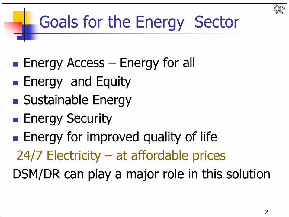
Goals for the Energy Sector

Energy Access – Energy for all

Energy and Equity

Sustainable Energy

Energy Security

Energy for improved quality of life

24/7 Electricity – at affordable prices

DSM/DR can play a major role in this solution

2

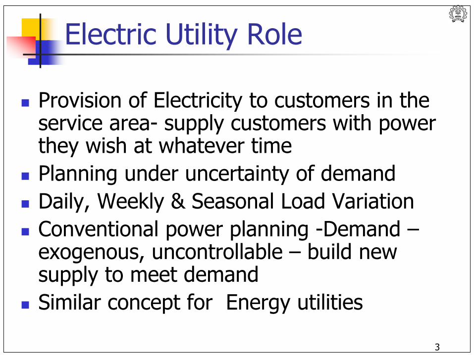
Electric Utility Role

Provision of Electricity to customers in the service area- supply customers with power they wish at whatever time

Planning under uncertainty of demand

Daily, Weekly & Seasonal Load Variation

Conventional power planning -Demand –exogenous, uncontrollable – build new supply to meet demand

Similar concept for Energy utilities

3

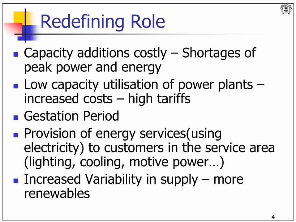
Redefining Role

Capacity additions costly – Shortages of peak power and energy

Low capacity utilisation of power plants –increased costs – high tariffs

Gestation Period

Provision of energy services(using electricity) to customers in the service area (lighting, cooling, motive power…)

Increased Variability in supply – more renewables

4

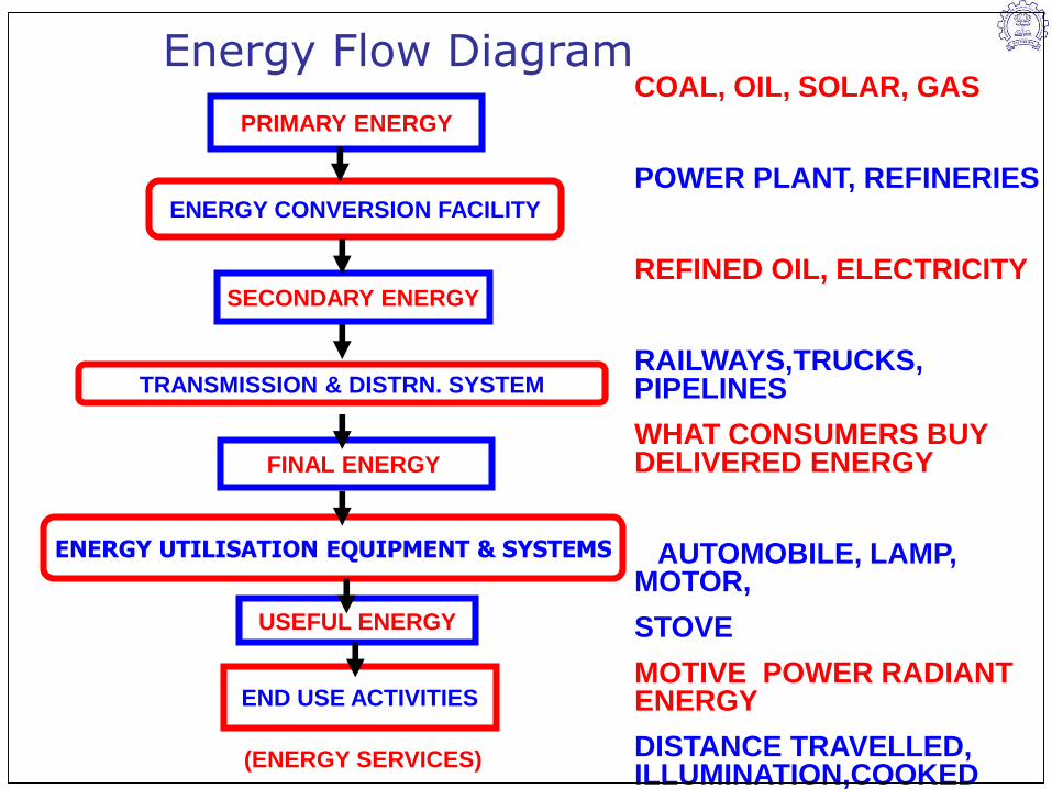
Energy Flow Diagram

PRIMARY ENERGY

ENERGY CONVERSION FACILITY

SECONDARY ENERGY

TRANSMISSION & DISTRN. SYSTEM

FINAL ENERGY

ENERGY UTILISATION EQUIPMENT & SYSTEMS

USEFUL ENERGY

END USE ACTIVITIES

(ENERGY SERVICES)

COAL, OIL, SOLAR, GAS

POWER PLANT, REFINERIES

REFINED OIL, ELECTRICITY

RAILWAYS,TRUCKS, PIPELINES

WHAT CONSUMERS BUY DELIVERED ENERGY

AUTOMOBILE, LAMP, MOTOR,

STOVE

MOTIVE POWER RADIANT ENERGY

DISTANCE TRAVELLED, ILLUMINATION,COOKED FOOD etc..

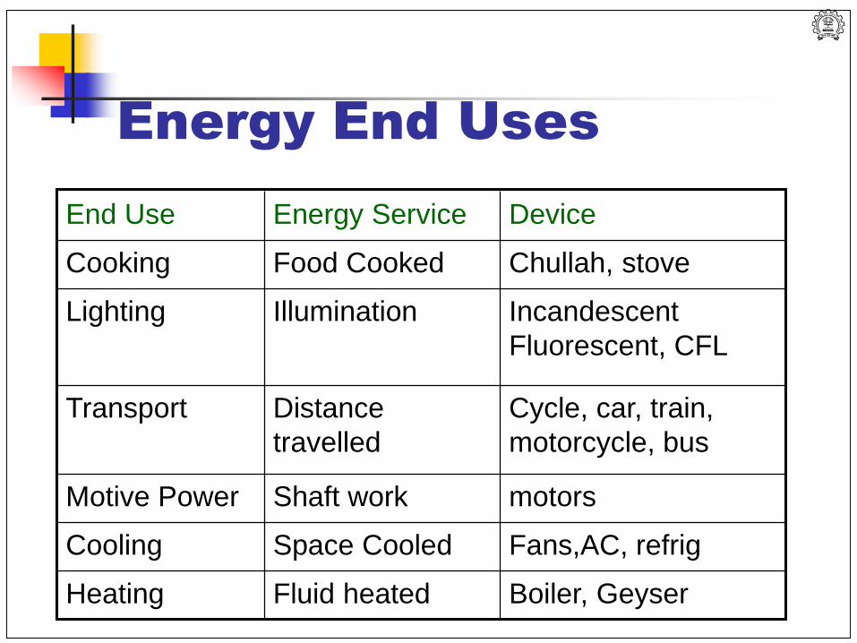
Energy End Uses

Boiler, GeyserFluid heatedHeating

Fans,AC, refrigSpace CooledCooling

motorsShaft workMotive Power

Cycle, car, train,

motorcycle, bus

Distance

travelled

Transport

Incandescent

Fluorescent, CFL

IlluminationLighting

Chullah, stoveFood CookedCooking

DeviceEnergy ServiceEnd Use

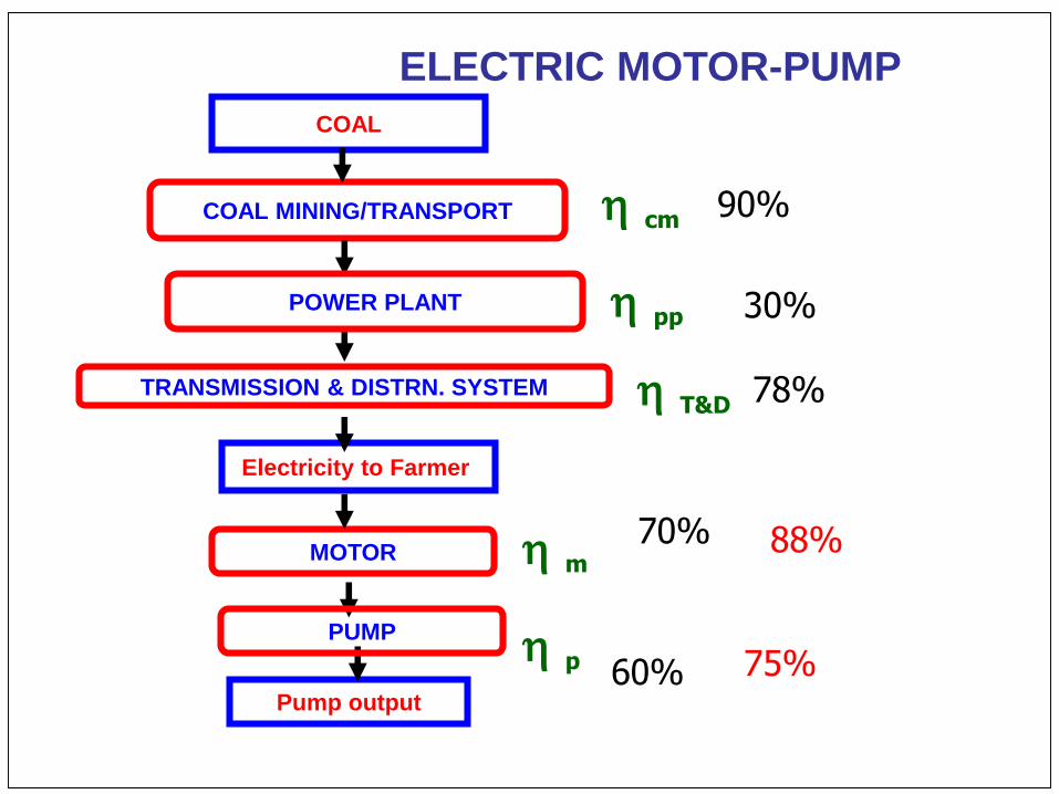
ELECTRIC MOTOR-PUMP

COAL

COAL MINING/TRANSPORT

TRANSMISSION & DISTRN. SYSTEM

Electricity to Farmer

MOTOR

Pump output

POWER PLANT

PUMP

cm

pp

T&D

m

p

90%

30%

78%

70%

60%

88%

75%

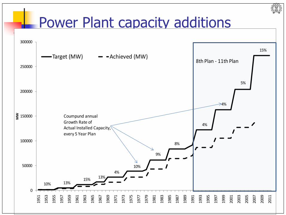
Power Plant capacity additions

0

50000

100000

150000

200000

250000

30000019

51

1953

1955

1957

1959

1961

1963

1965

1967

1969

1971

1973

1975

1977

1979

1981

1983

1985

1987

1989

1991

1993

1995

1997

1999

2001

2003

2005

2007

2009

2011

MW

Target (MW) Achieved (MW)8th Plan - 11th Plan

10% 13%15%

13%4%

4%

4%

8%

9%

10%

5%

15%

Coumpund annual Growth Rate of Actual Installed Capacity,every 5 Year Plan

0

200

400

600

800

1000

1200

1400

GW

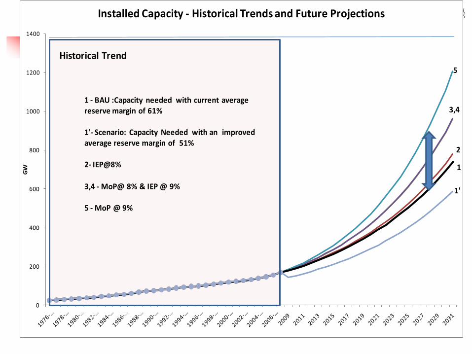
Installed Capacity - Historical Trends and Future Projections

Historical Trend

5

3,4

2

1 - BAU :Capacity needed with current average reserve margin of 61%

1'- Scenario: Capacity Needed with an improved average reserve margin of 51%

2- IEP@8%

3,4 - MoP@ 8% & IEP @ 9%

5 - MoP @ 9%

1'

1

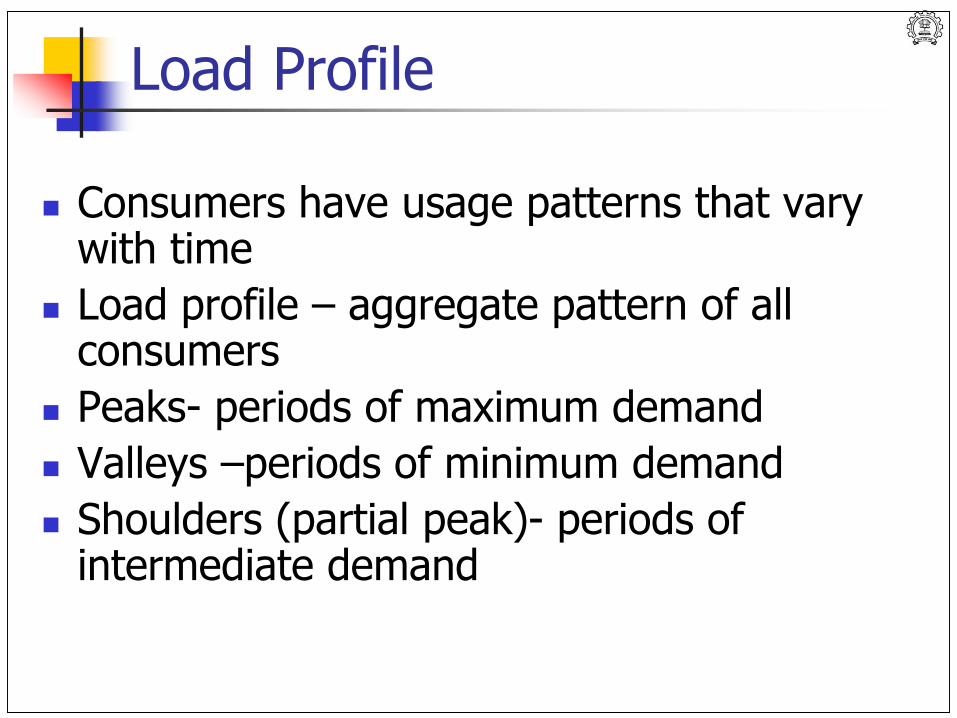
Load Profile

Consumers have usage patterns that vary with time

Load profile – aggregate pattern of all consumers

Peaks- periods of maximum demand

Valleys –periods of minimum demand

Shoulders (partial peak)- periods of intermediate demand

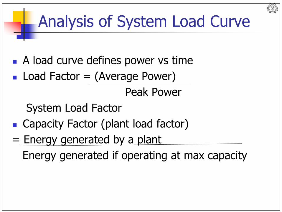
Analysis of System Load Curve

A load curve defines power vs time

Load Factor = (Average Power)

Peak Power

System Load Factor

Capacity Factor (plant load factor)

= Energy generated by a plant

Energy generated if operating at max capacity

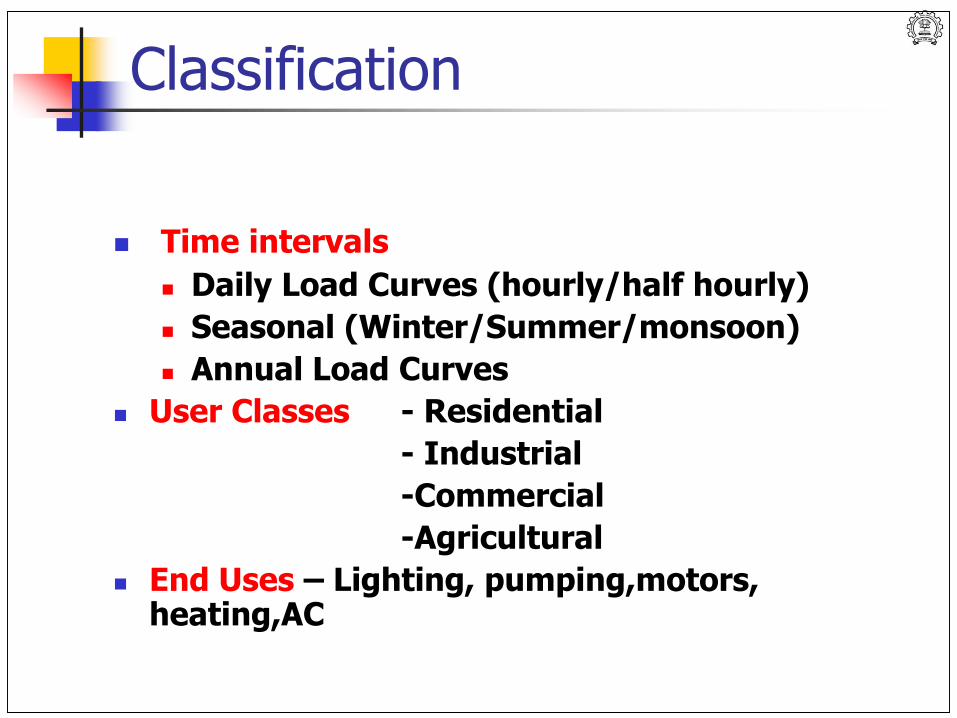
Classification

Time intervals

Daily Load Curves (hourly/half hourly)

Seasonal (Winter/Summer/monsoon)

Annual Load Curves

User Classes - Residential

- Industrial

-Commercial

-Agricultural

End Uses – Lighting, pumping,motors, heating,AC

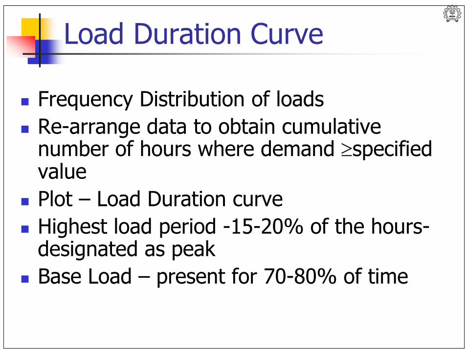
Load Duration Curve

Frequency Distribution of loads

Re-arrange data to obtain cumulative number of hours where demand specified value

Plot – Load Duration curve

Highest load period -15-20% of the hours-designated as peak

Base Load – present for 70-80% of time

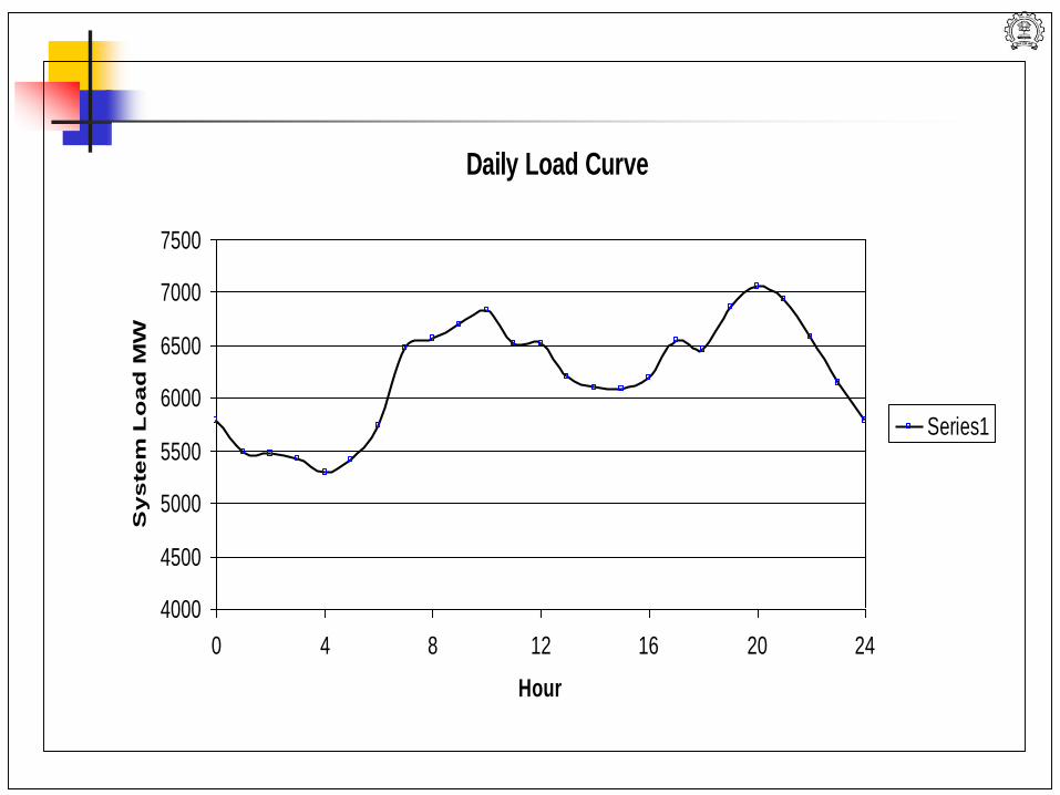
Daily Load Curve

4000

4500

5000

5500

6000

6500

7000

7500

0 4 8 12 16 20 24

Hour

Sy

ste

m L

oa

d M

W

Series1

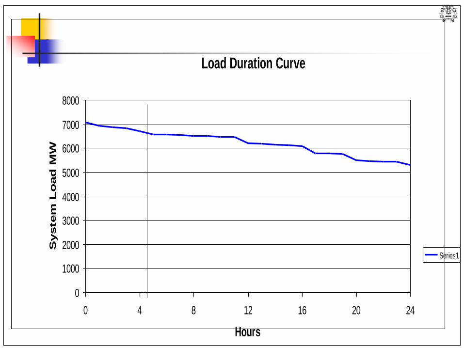
Load Duration Curve

0

1000

2000

3000

4000

5000

6000

7000

8000

0 4 8 12 16 20 24

Hours

System

Lo

ad

MW

Series1

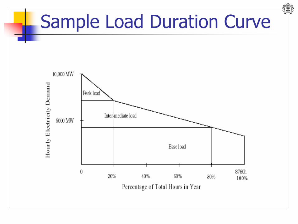
Sample Load Duration Curve

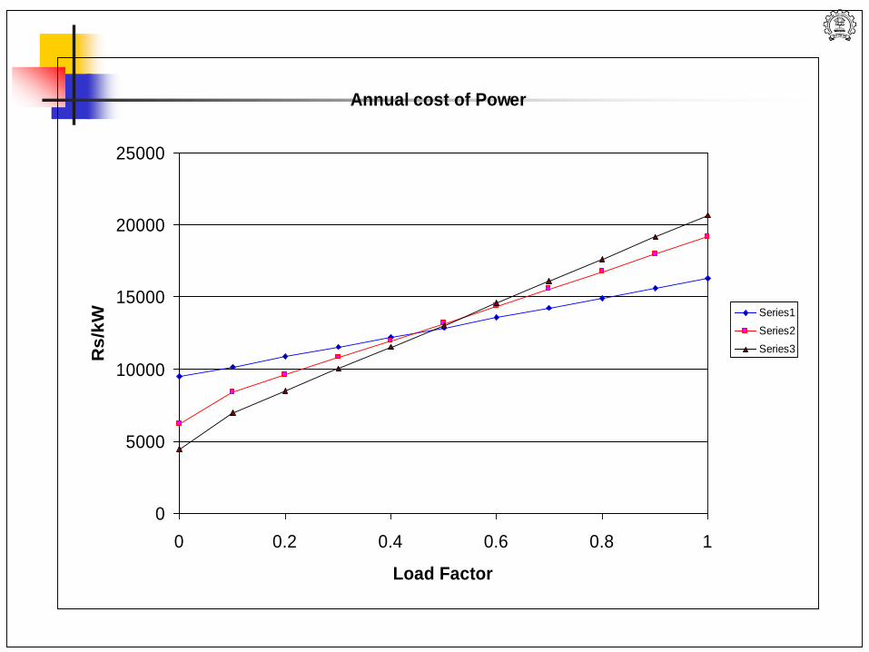
Annual cost of Power

0

5000

10000

15000

20000

25000

0 0.2 0.4 0.6 0.8 1

Load Factor

Rs

/kW Series1

Series2

Series3

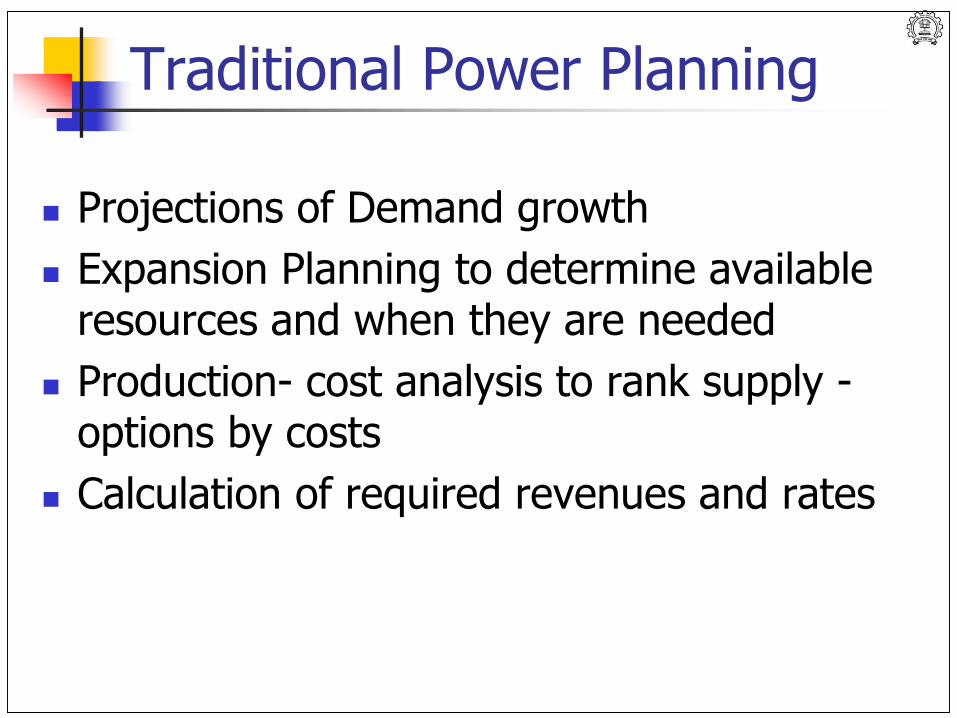
Traditional Power Planning

Projections of Demand growth

Expansion Planning to determine available resources and when they are needed

Production- cost analysis to rank supply -options by costs

Calculation of required revenues and rates

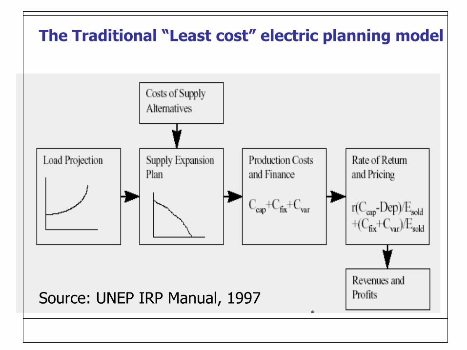
The Traditional “Least cost” electric planning model

Source: UNEP IRP Manual, 1997

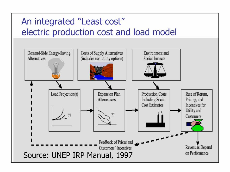
An integrated “Least cost”electric production cost and load model


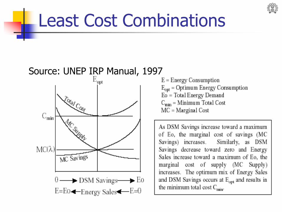
Least Cost Combinations


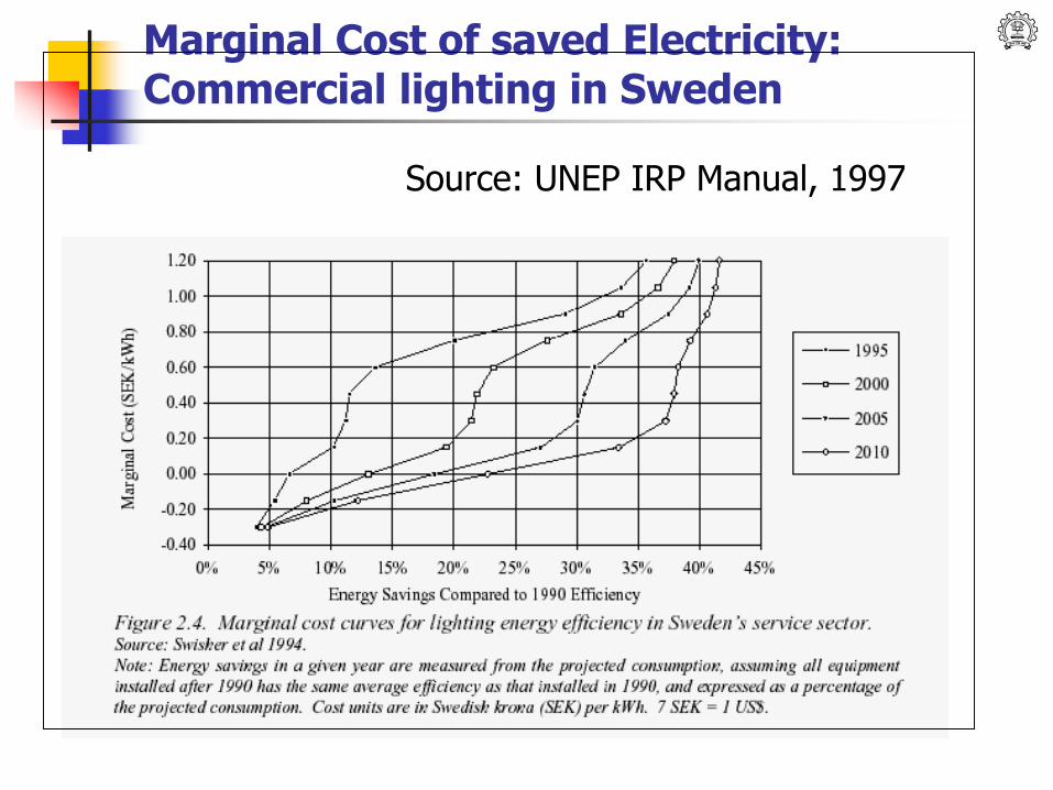
Marginal Cost of saved Electricity: Commercial lighting in Sweden


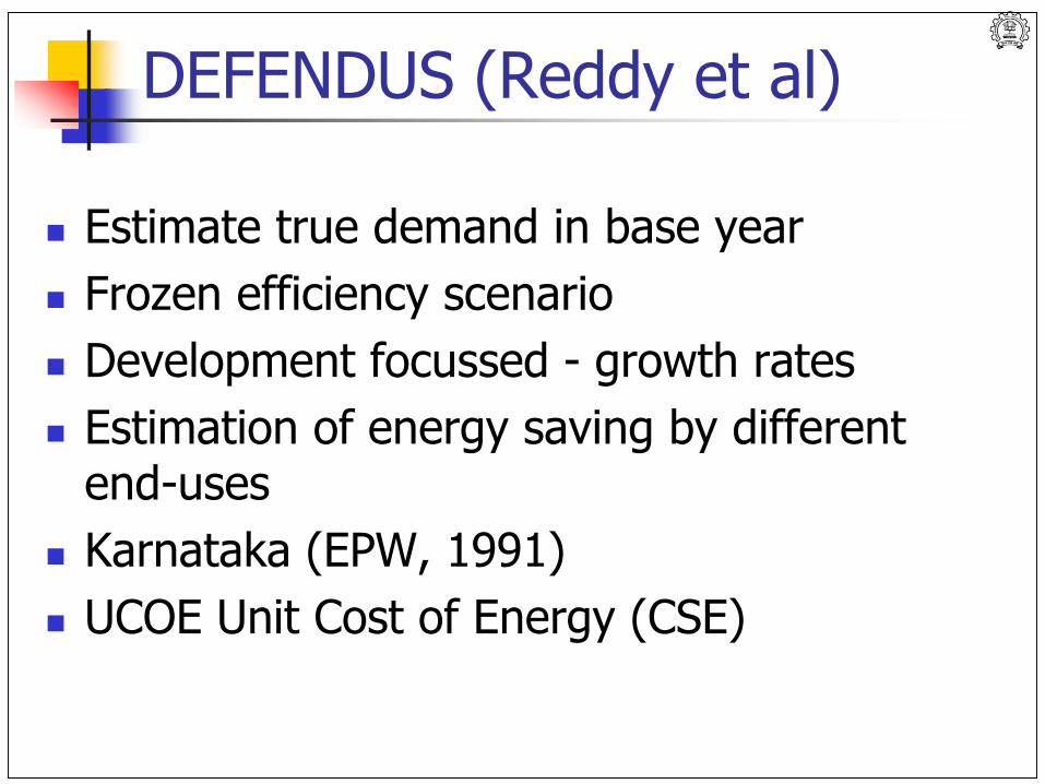
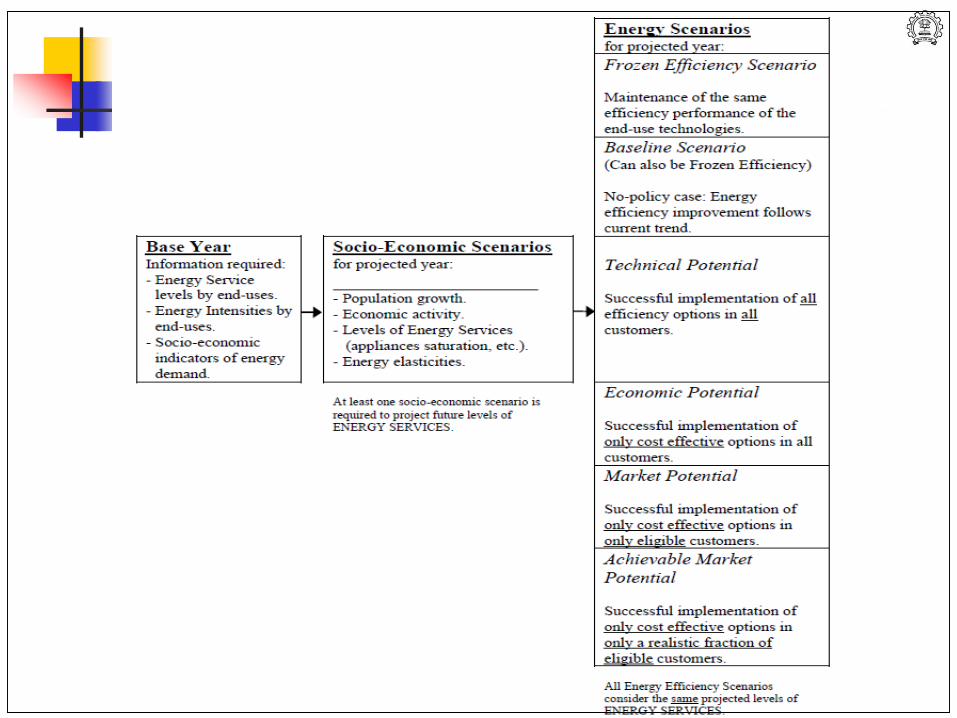
DEFENDUS (Reddy et al)

Estimate true demand in base year

Frozen efficiency scenario

Development focussed - growth rates

Estimation of energy saving by different end-uses

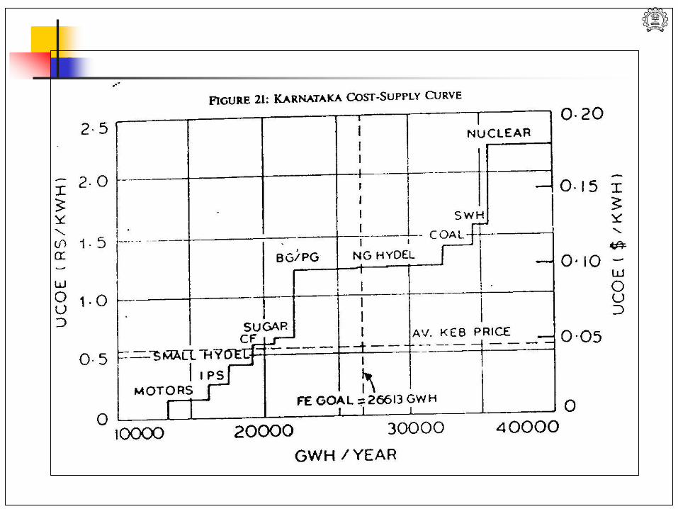
Karnataka (EPW, 1991)

UCOE Unit Cost of Energy (CSE)

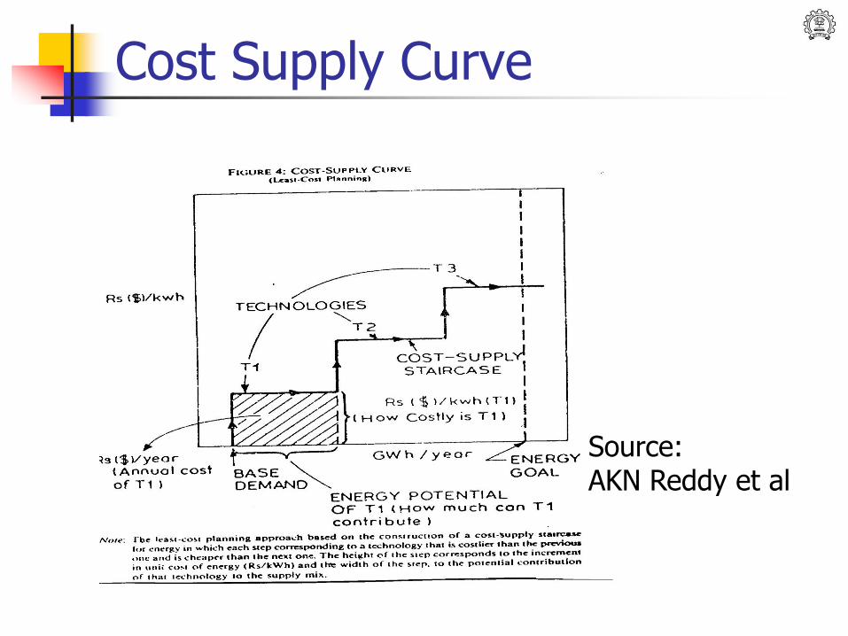
Cost Supply Curve

Source: AKN Reddy et al

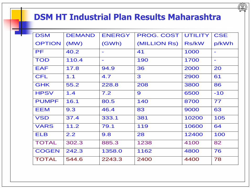
DSM

OPTION

DEMAND

(MW)

ENERGY

(GWh)

PROG. COST

(MILLION Rs)

UTILITY

Rs/kW

CSE

p/kWh

PF 40.2 - 41 1000 -

TOD 110.4 - 190 1700 -

EAF 17.8 94.9 36 2000 20

CFL 1.1 4.7 3 2900 61

GHK 55.2 228.8 208 3800 86

HPSV 1.4 7.2 9 6500 -10

PUMPF 16.1 80.5 140 8700 77

EEM 9.3 46.4 83 9000 63

VSD 37.4 333.1 381 10200 105

VARS 11.2 79.1 119 10600 64

ELB 2.2 9.8 28 12400 100

TOTAL 302.3 885.3 1238 4100 82

COGEN 242.3 1358.0 1162 4800 76

TOTAL 544.6 2243.3 2400 4400 78

DSM HT Industrial Plan Results Maharashtra

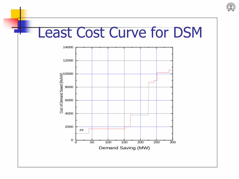
0 50 100 150 200 250 3000

2000

4000

6000

8000

10000

12000

14000

Pf

Cos

t of D

eman

d S

aved

(Rs/

kW)

Demand Saving (MW)

Least Cost Curve for DSM

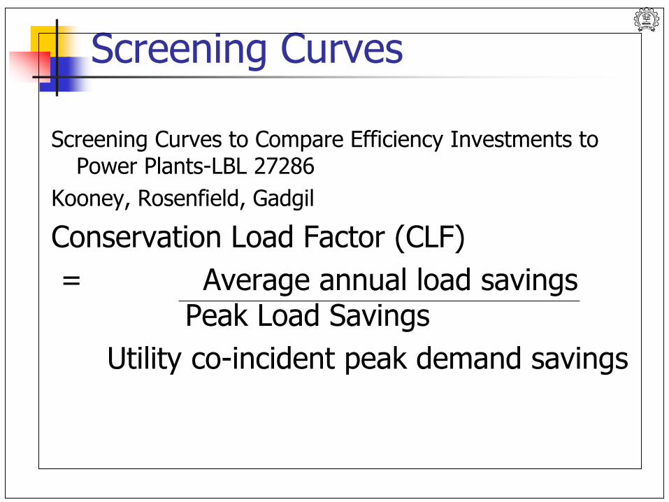
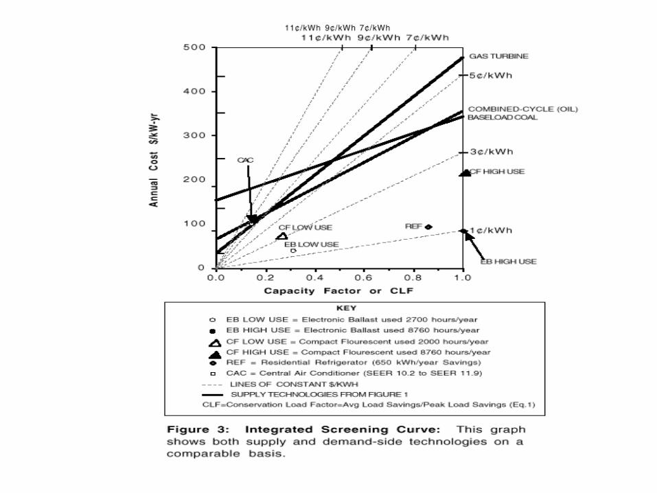
Screening Curves

Screening Curves to Compare Efficiency Investments to Power Plants-LBL 27286

Kooney, Rosenfield, Gadgil

Conservation Load Factor (CLF)

= Average annual load savingsPeak Load Savings

Utility co-incident peak demand savings

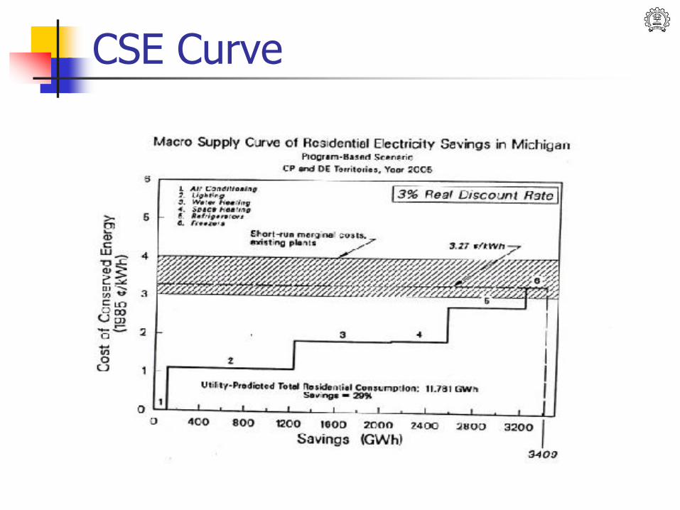
CSE Curve

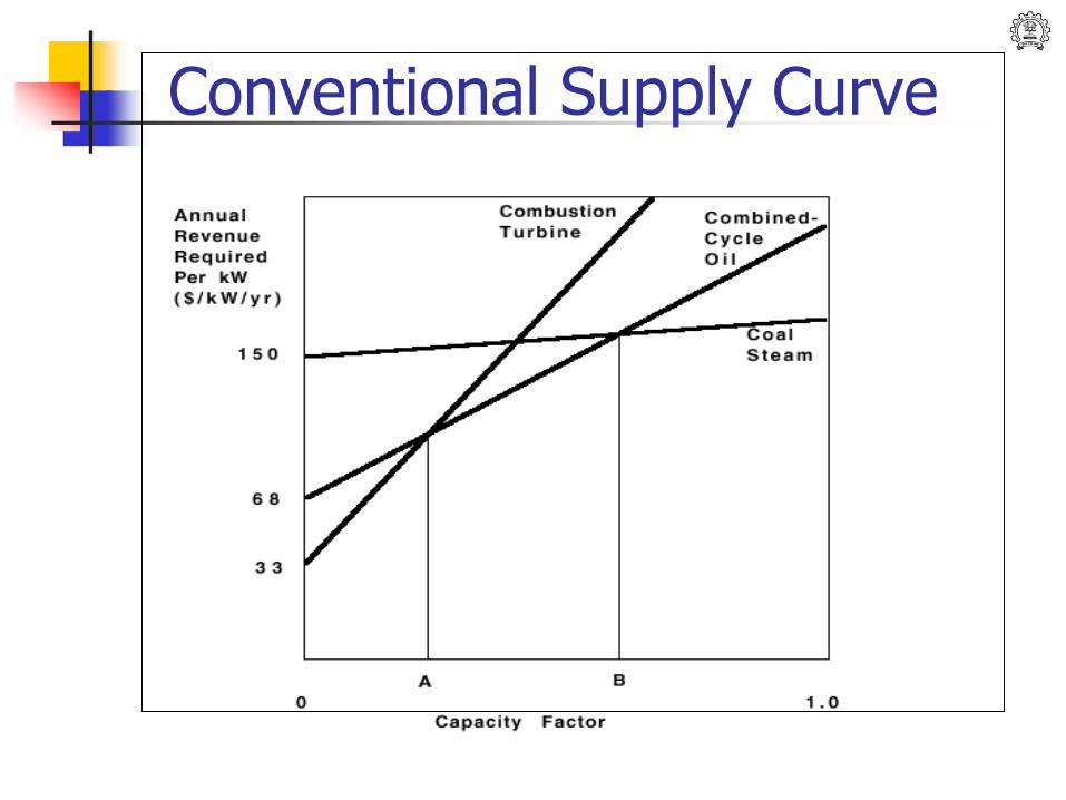
Conventional Supply Curve

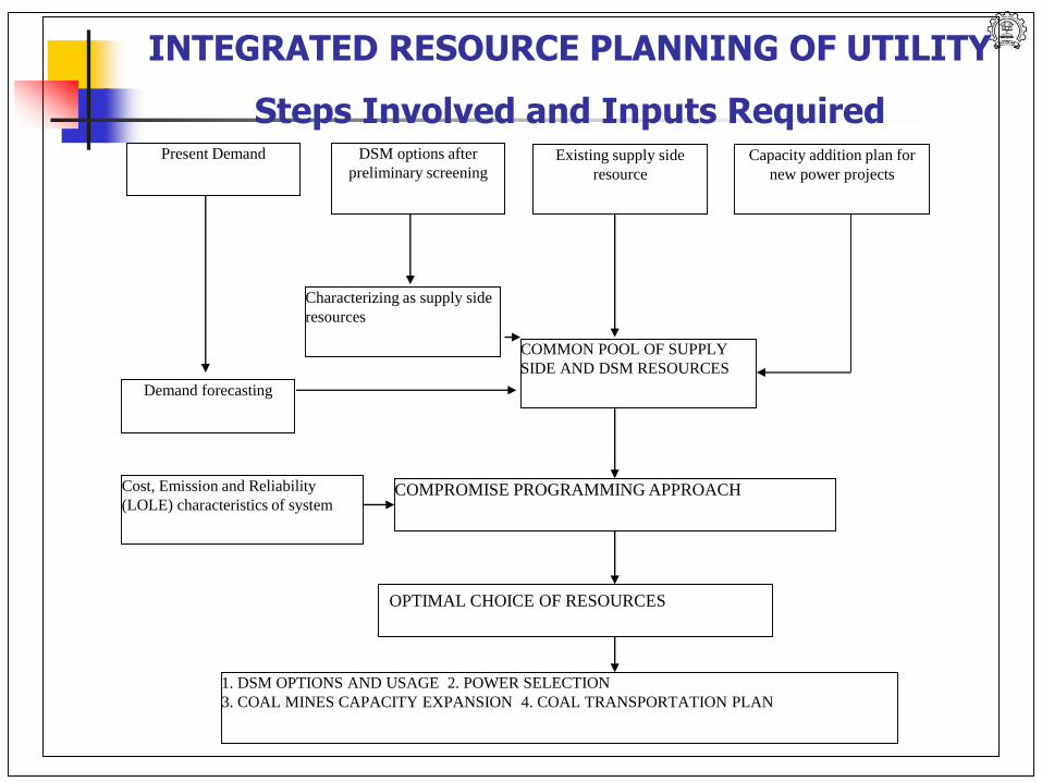
Present Demand DSM options after

preliminary screeningExisting supply side

resource

Capacity addition plan for

new power projects

Demand forecasting

Characterizing as supply side

resources

COMMON POOL OF SUPPLY

SIDE AND DSM RESOURCES

Cost, Emission and Reliability

(LOLE) characteristics of systemCOMPROMISE PROGRAMMING APPROACH

OPTIMAL CHOICE OF RESOURCES

1. DSM OPTIONS AND USAGE 2. POWER SELECTION

3. COAL MINES CAPACITY EXPANSION 4. COAL TRANSPORTATION PLAN

INTEGRATED RESOURCE PLANNING OF UTILITY

Steps Involved and Inputs Required

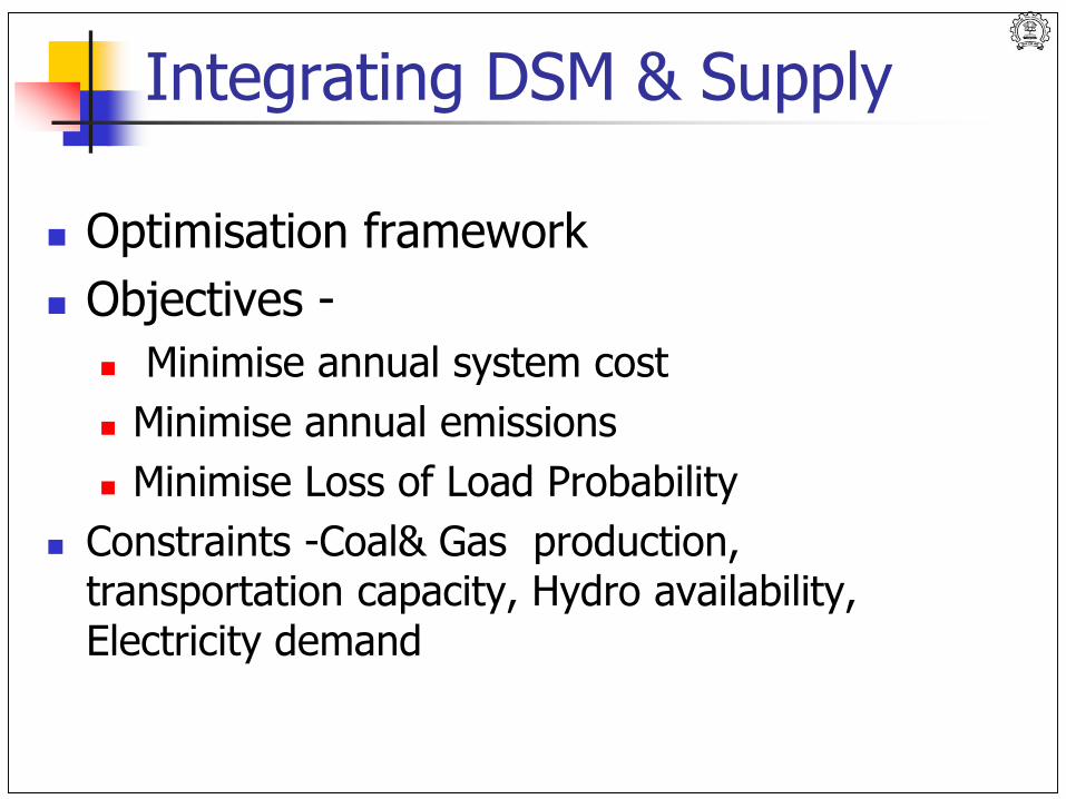
Integrating DSM & Supply

Optimisation framework

Objectives -

Minimise annual system cost

Minimise annual emissions

Minimise Loss of Load Probability

Constraints -Coal& Gas production, transportation capacity, Hydro availability, Electricity demand

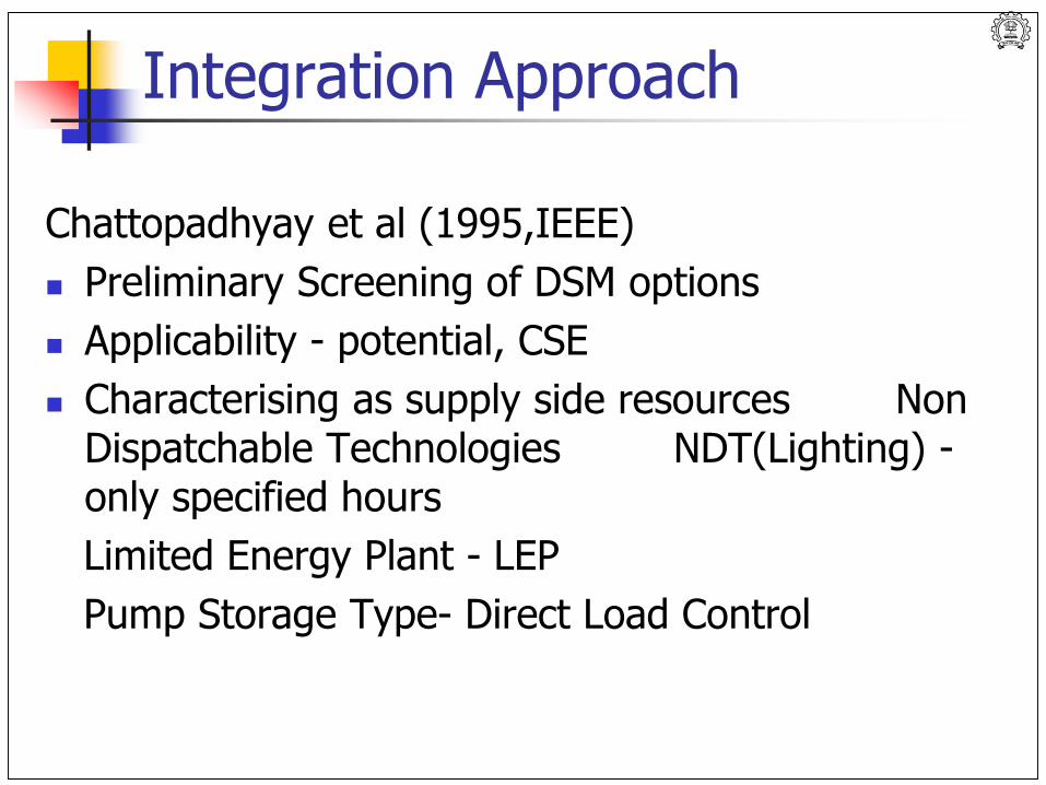
Integration Approach

Chattopadhyay et al (1995,IEEE)

Preliminary Screening of DSM options

Applicability - potential, CSE

Characterising as supply side resources Non Dispatchable Technologies NDT(Lighting) -only specified hours

Limited Energy Plant - LEP

Pump Storage Type- Direct Load Control

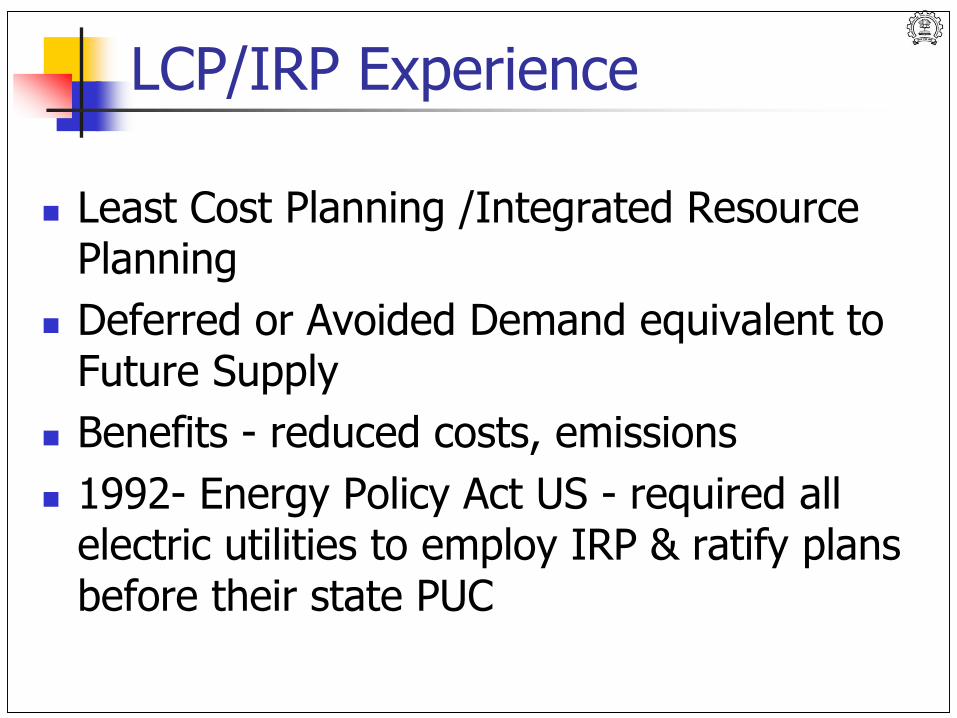
LCP/IRP Experience

Least Cost Planning /Integrated Resource Planning

Deferred or Avoided Demand equivalent to Future Supply

Benefits - reduced costs, emissions

1992- Energy Policy Act US - required all electric utilities to employ IRP & ratify plans before their state PUC

What is Demand Side Management?

Why Demand Side Management?

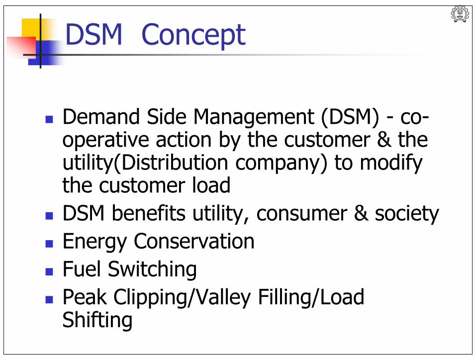
DSM Concept

Demand Side Management (DSM) - co-operative action by the customer & the utility(Distribution company) to modify the customer load

DSM benefits utility, consumer & society

Energy Conservation

Fuel Switching

Peak Clipping/Valley Filling/Load Shifting

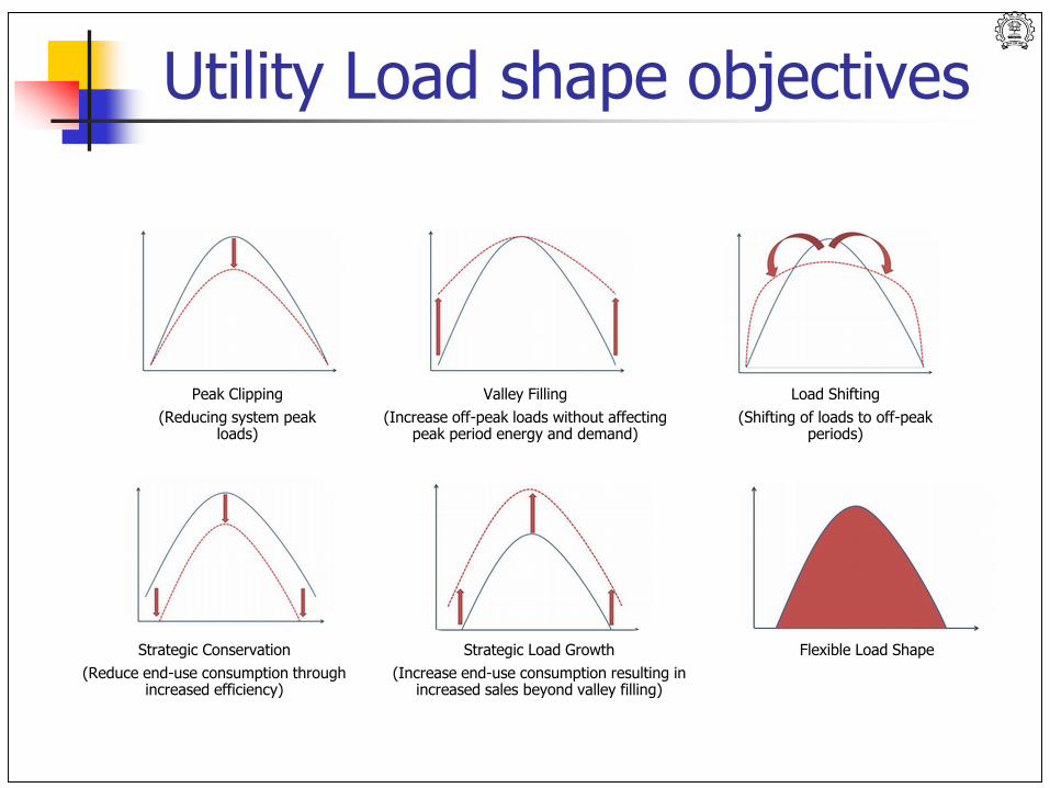
Utility Load shape objectives

Peak Clipping

(Reducing system peak loads)

Valley Filling

(Increase off-peak loads without affecting peak period energy and demand)

Load Shifting

(Shifting of loads to off-peak periods)

Strategic Conservation

(Reduce end-use consumption through increased efficiency)

Strategic Load Growth

(Increase end-use consumption resulting in increased sales beyond valley filling)

Flexible Load Shape

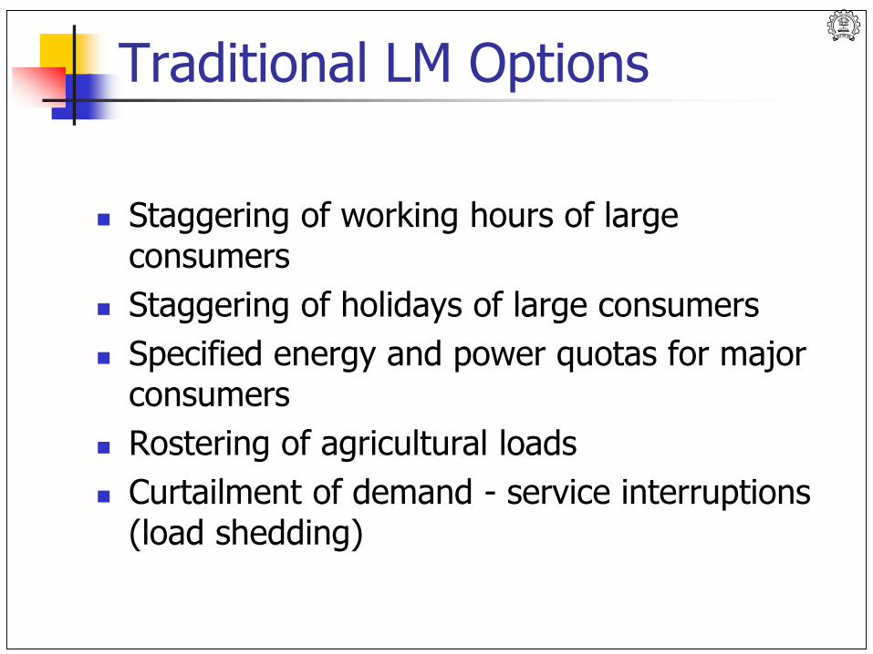
Traditional LM Options

Staggering of working hours of large consumers

Staggering of holidays of large consumers

Specified energy and power quotas for major consumers

Rostering of agricultural loads

Curtailment of demand - service interruptions (load shedding)

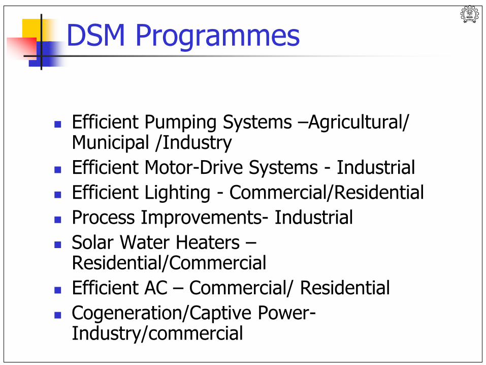
DSM Programmes

Efficient Pumping Systems –Agricultural/ Municipal /Industry

Efficient Motor-Drive Systems - Industrial

Efficient Lighting - Commercial/Residential

Process Improvements- Industrial

Solar Water Heaters –Residential/Commercial

Efficient AC – Commercial/ Residential

Cogeneration/Captive Power-Industry/commercial

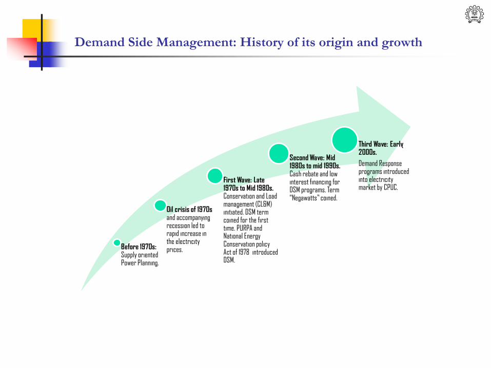
Demand Side Management: History of its origin and growth

Before 1970s: Supply oriented Power Planning.

Oil crisis of 1970s and accompanying recession led to rapid increase in the electricity prices.

First Wave: Late 1970s to Mid 1980s. Conservation and Load management (CL&M) initiated. DSM term coined for the first time. PURPA and National Energy Conservation policy Act of 1978 introduced DSM.

Second Wave: Mid 1980s to mid 1990s. Cash rebate and low interest financing for DSM programs. Term “Negawatts” coined.

Third Wave: Early 2000s.

Demand Response programs introduced into electricity market by CPUC.

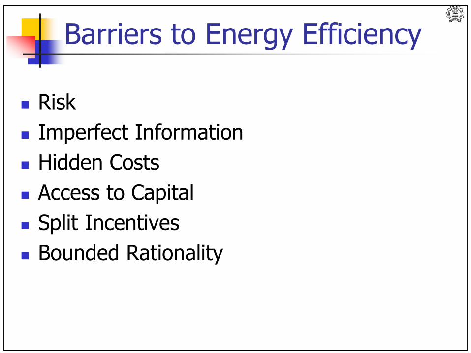
Barriers to Energy Efficiency

Risk

Imperfect Information

Hidden Costs

Access to Capital

Split Incentives

Bounded Rationality

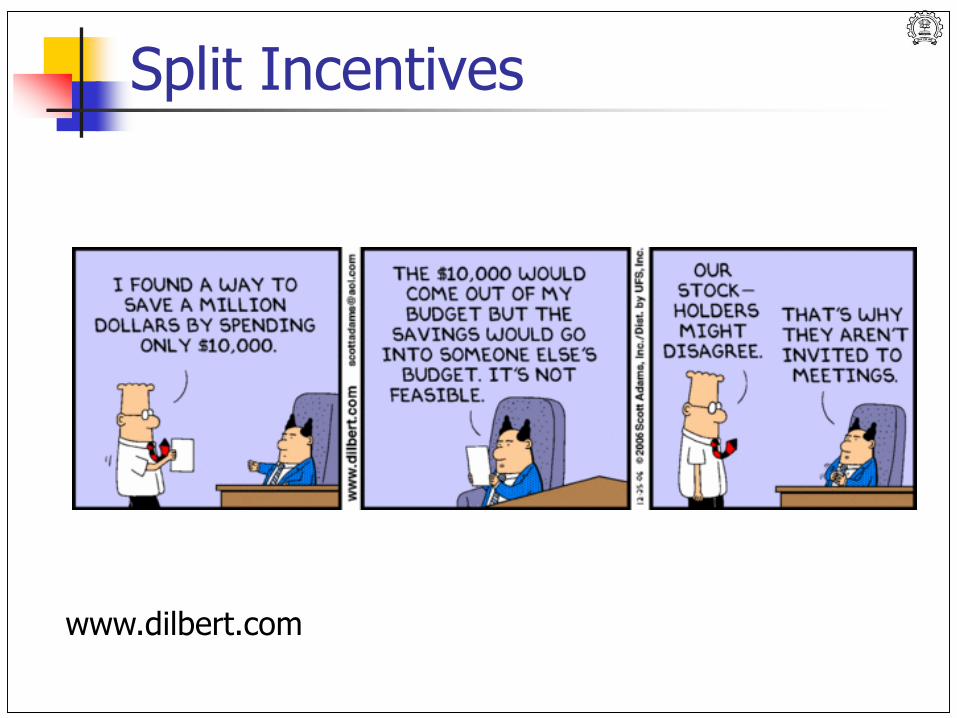
Split Incentives

www.dilbert.com

Early ESCO concept

"We will leave a steam engine free of charge to you. We will install these and will take over for five years the customer service. We guarantee you that the coal for the machine costs less, than you must spend at present at fodder (energy) on the horses, which do the same work. And everything that we require of you, is that you give us a third of the money, which you save.“

[James Watt, 1736-1819]

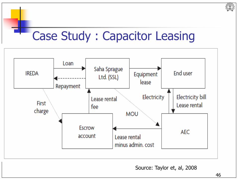
Case Study : Capacitor Leasing

46

Source: Taylor et, al, 2008

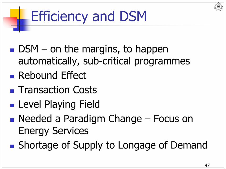
Efficiency and DSM

DSM – on the margins, to happen automatically, sub-critical programmes

Rebound Effect

Transaction Costs

Level Playing Field

Needed a Paradigm Change – Focus on Energy Services

Shortage of Supply to Longage of Demand

47

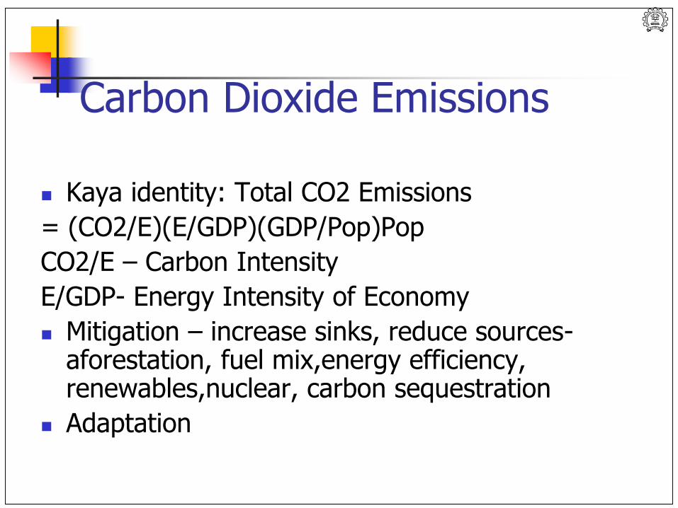
Carbon Dioxide Emissions

Kaya identity: Total CO2 Emissions

= (CO2/E)(E/GDP)(GDP/Pop)Pop

CO2/E – Carbon Intensity

E/GDP- Energy Intensity of Economy

Mitigation – increase sinks, reduce sources-aforestation, fuel mix,energy efficiency, renewables,nuclear, carbon sequestration

Adaptation

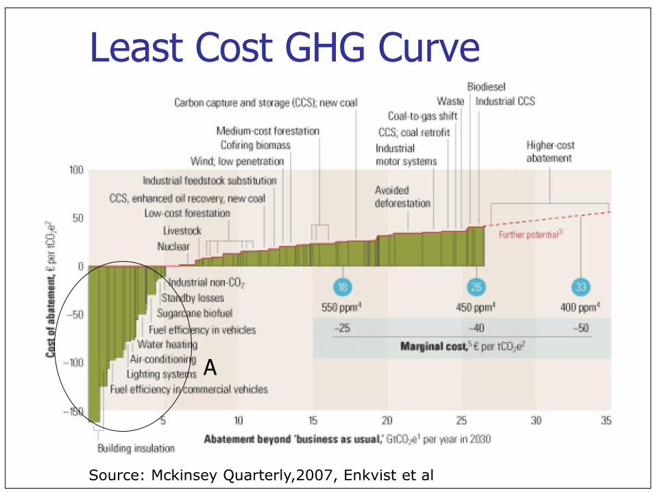
Least Cost GHG Curve

Source: Mckinsey Quarterly,2007, Enkvist et al

A

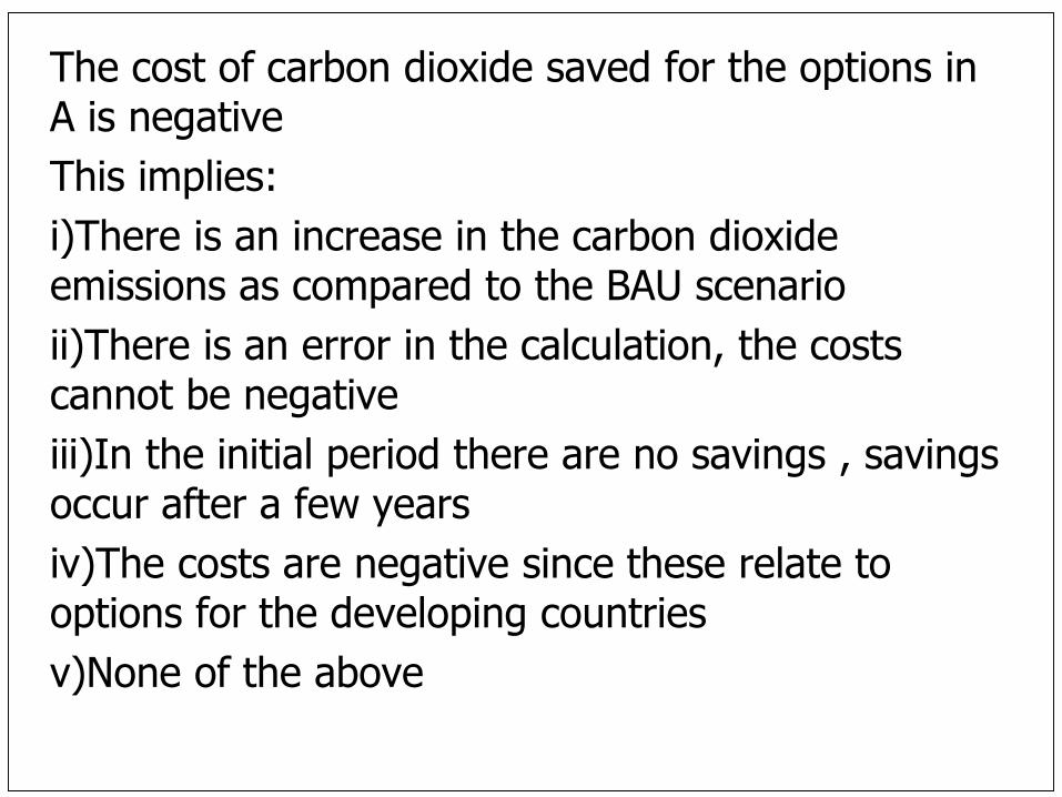
The cost of carbon dioxide saved for the options in A is negative

This implies:

i)There is an increase in the carbon dioxide emissions as compared to the BAU scenario

ii)There is an error in the calculation, the costs cannot be negative

iii)In the initial period there are no savings , savings occur after a few years

iv)The costs are negative since these relate to options for the developing countries

v)None of the above

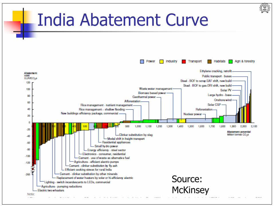
India Abatement Curve

Source: McKinsey

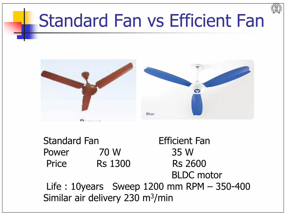
Standard Fan vs Efficient Fan

Standard Fan Efficient FanPower 70 W 35 WPrice Rs 1300 Rs 2600

BLDC motorLife : 10years Sweep 1200 mm RPM – 350-400Similar air delivery 230 m3/min

Cost Of Saved Energy – Efficient Fan

53

0

2

4

6

8

10

12

14

16

18

0 0.1 0.2 0.3 0.4 0.5

CSERs/kWh

Discount Rate

1000 hours

2000 hours

4000 hours

3000 hours

Macro-Level Barriers

Distorted Energy Prices

Lack of Human Capital Infrastructure

Lack of Technical Infrastructure

Lock-in effects

Lack of External access to Capital

Institutional Factors

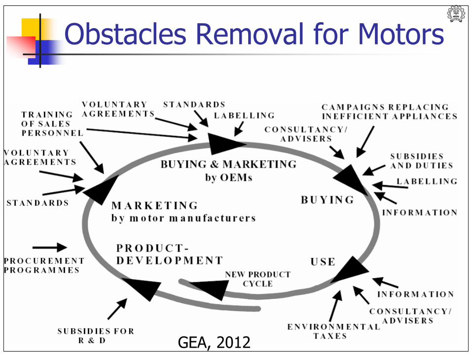
Obstacles Removal for Motors

GEA, 2012

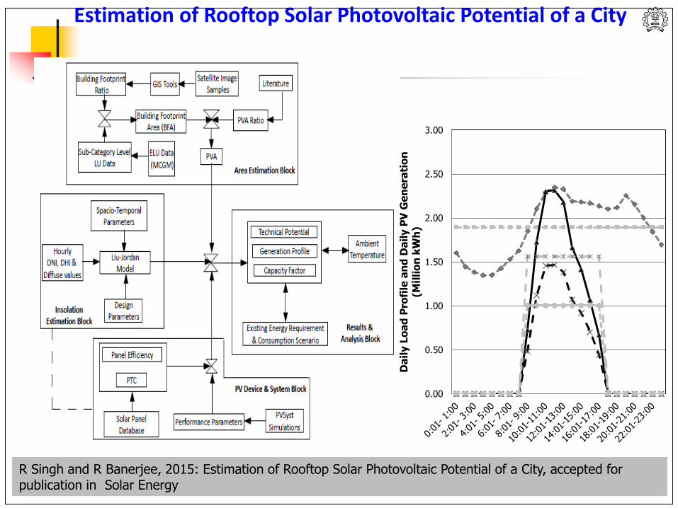
Estimation of Rooftop Solar Photovoltaic Potential of a City

R Singh and R Banerjee, 2015: Estimation of Rooftop Solar Photovoltaic Potential of a City, accepted for publication in Solar Energy

0.00

0.50

1.00

1.50

2.00

2.50

3.00

Da

ily L

oa

d P

rofi

le a

nd

Da

ily P

V G

en

era

tio

n(M

illi

on

kW

h)

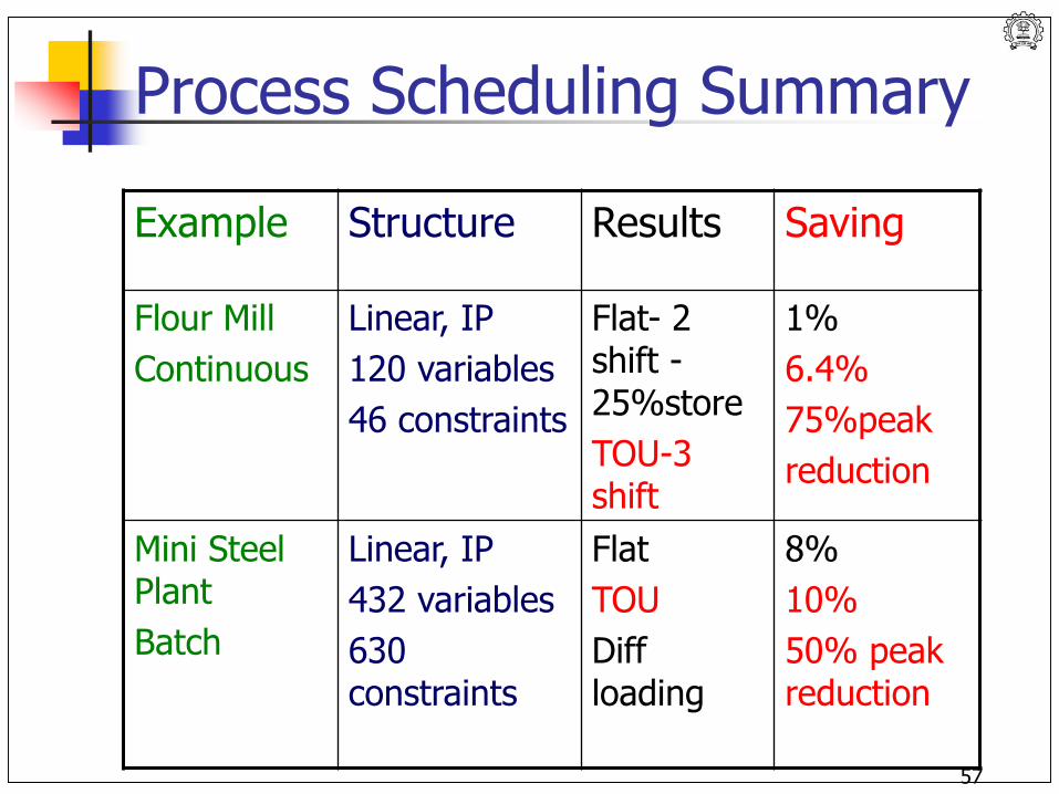
Process Scheduling Summary

Example Structure Results Saving

Flour Mill

Continuous

Linear, IP

120 variables

46 constraints

Flat- 2 shift -25%store

TOU-3 shift

1%

6.4%

75%peak

reduction

Mini Steel Plant

Batch

Linear, IP

432 variables

630 constraints

Flat

TOU

Diff loading

8%

10%

50% peak reduction

57

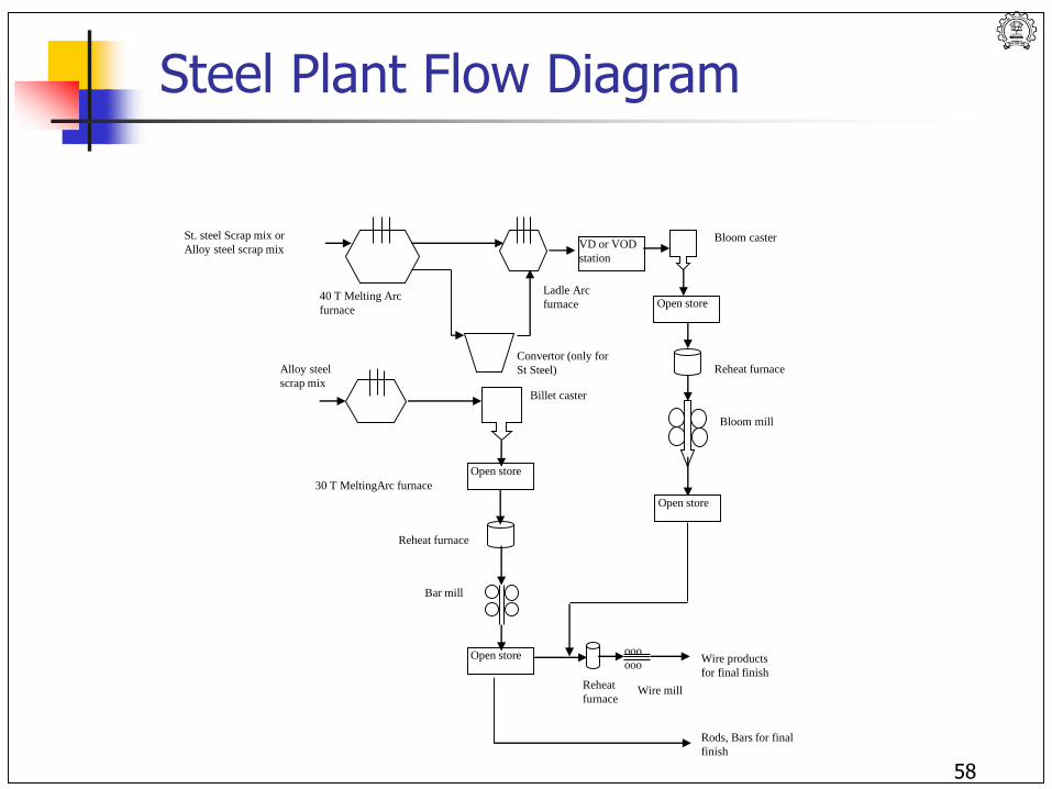
30 T MeltingArc furnace

Bar mill

Wire mill

40 T Melting Arc

furnace

St. steel Scrap mix or

Alloy steel scrap mix

Alloy steel

scrap mix

Convertor (only for

St Steel)

Ladle Arc

furnace

VD or VOD

station

Bloom caster

Billet caster

Bloom mill

ooo

ooo

Reheat furnace

Reheat furnace

Reheat

furnace

Wire products

for final finish

Rods, Bars for final

finish

Open store

Open store

Open store

Open store

Steel Plant Flow Diagram

58

0

10

20

30

40

50

60

Time hours

Lo

ad

MW

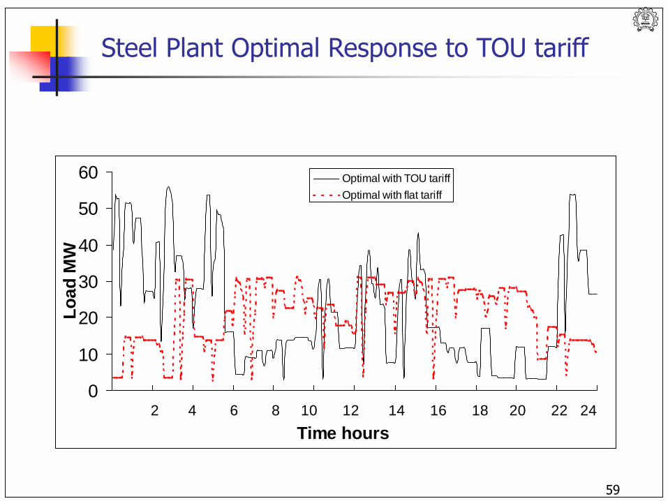
Optimal with TOU tariff

Optimal with flat tariff

2 4 6 8 10 12 14 16 18 20 22 24

Steel Plant Optimal Response to TOU tariff

59

Process Scheduling Summary

Example Structure Results Saving

Flour Mill

Continuous

Linear, IP

120 variables

46 constraints

Flat- 2 shift -25%store

TOU-3 shift

1%

6.4%

75%peak

reduction

Mini Steel Plant

Batch

Linear, IP

432 variables

630 constraints

Flat

TOU

Diff loading

8%

10%

50% peak reduction

60

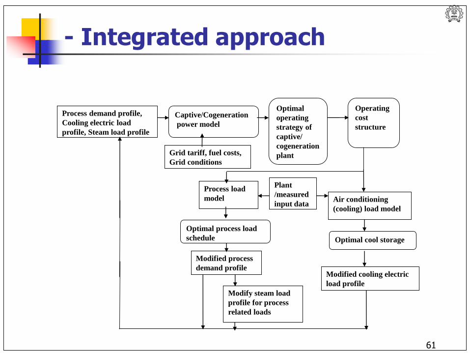
- Integrated approach

Operating

cost

structure

Optimal

operating

strategy of

captive/

cogeneration

plant

Captive/Cogeneration

power model

Grid tariff, fuel costs,

Grid conditions

Modified process

demand profile

Process demand profile,

Cooling electric load

profile, Steam load profile

Process load

model Air conditioning

(cooling) load model

Optimal process load

schedule Optimal cool storage

Plant

/measured

input data

Modified cooling electric

load profile

Modify steam load

profile for process

related loads

61

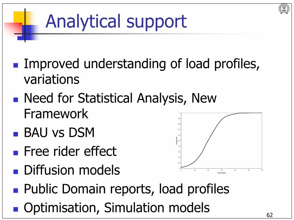
Analytical support

Improved understanding of load profiles, variations

Need for Statistical Analysis, New Framework

BAU vs DSM

Free rider effect

Diffusion models

Public Domain reports, load profiles

Optimisation, Simulation models

0

0.1

0.2

0.3

0.4

0.5

0.6

0.7

0.8

0.9

1

0 10 20 30 40 50 60

Fra

cti

on

(f)

Time (Years)

62

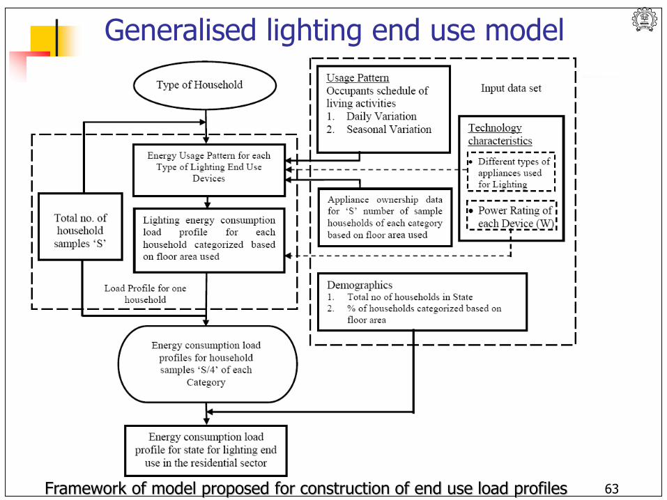
Generalised lighting end use model

Framework of model proposed for construction of end use load profiles 63

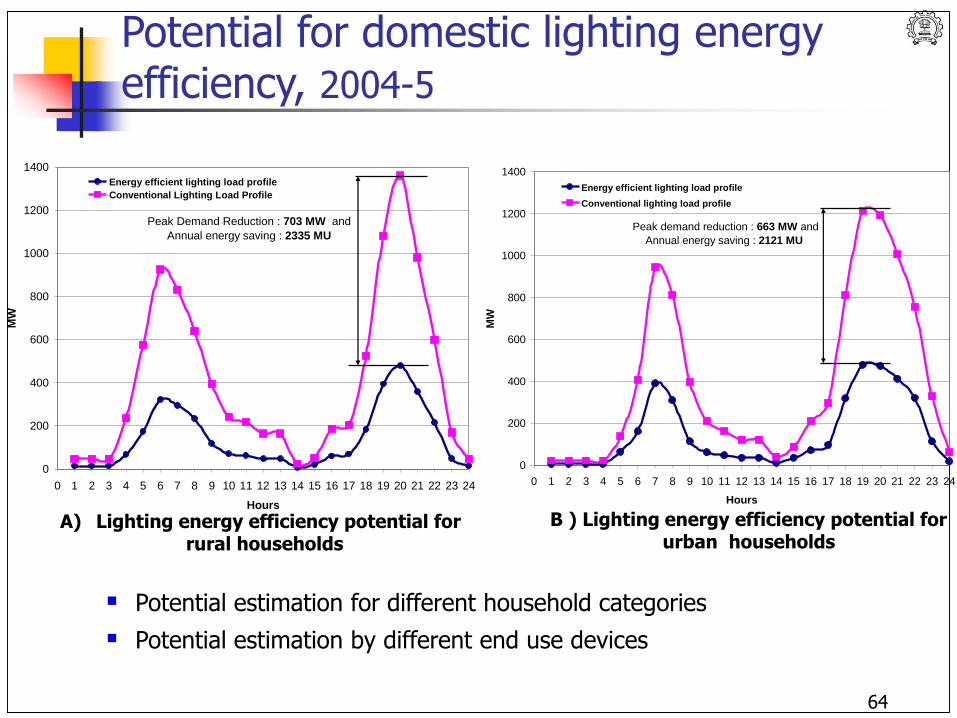
Potential for domestic lighting energy efficiency, 2004-5

Potential estimation for different household categories

Potential estimation by different end use devices

0

200

400

600

800

1000

1200

1400

0 1 2 3 4 5 6 7 8 9 10 11 12 13 14 15 16 17 18 19 20 21 22 23 24

Hours

MW

Energy efficient lighting load profile

Conventional Lighting Load Profile

Peak Demand Reduction : 703 MW and

Annual energy saving : 2335 MU

0

200

400

600

800

1000

1200

1400

0 1 2 3 4 5 6 7 8 9 10 11 12 13 14 15 16 17 18 19 20 21 22 23 24

HoursM

W

Energy efficient lighting load profile

Conventional lighting load profile

Peak demand reduction : 663 MW and

Annual energy saving : 2121 MU

A) Lighting energy efficiency potential forrural households

B ) Lighting energy efficiency potential forurban households

64

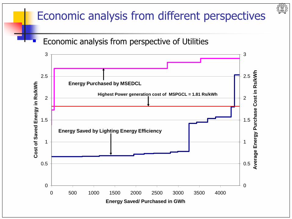
Economic analysis from different perspectives

Economic analysis from perspective of Utilities

0

0.5

1

1.5

2

2.5

3

0 500 1000 1500 2000 2500 3000 3500 4000

Energy Saved/ Purchased in GWh

Co

st

of

Saved

En

erg

y in

Rs/k

Wh

0

0.5

1

1.5

2

2.5

3

Avera

ge E

nerg

y P

urc

hase C

ost

in R

s/k

Wh

Energy Purchased by MSEDCL

Energy Saved by Lighting Energy Efficiency

Highest Power generation cost of MSPGCL = 1.81 Rs/kWh

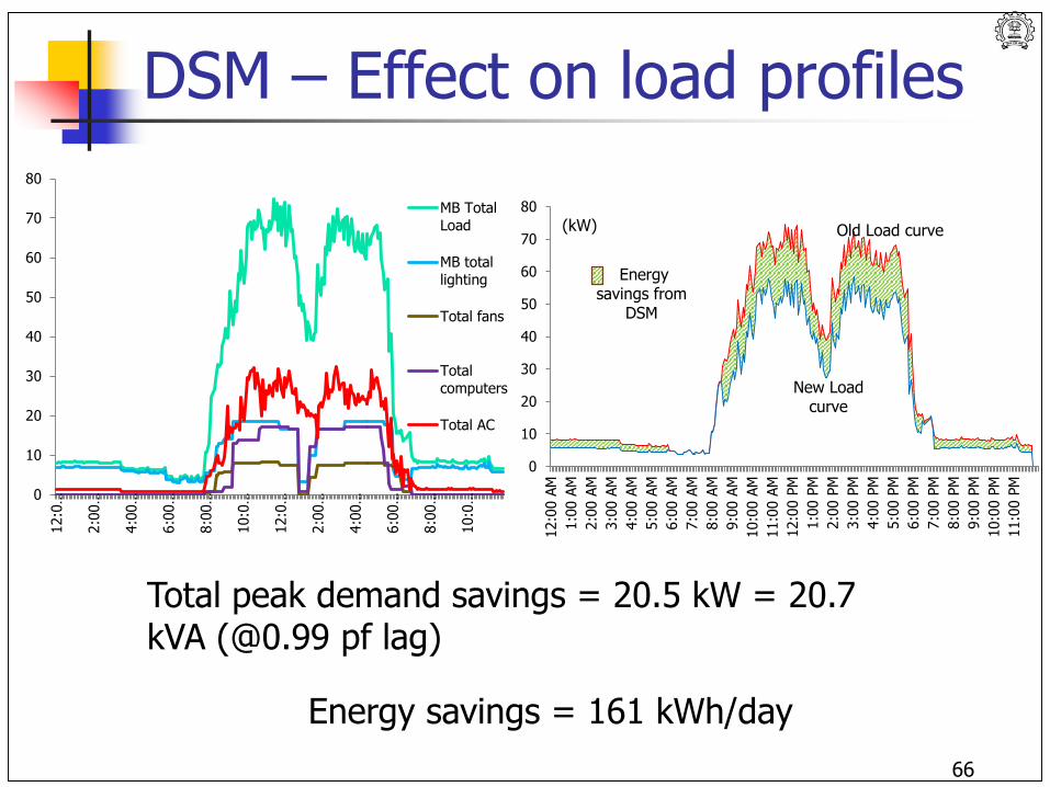
DSM – Effect on load profiles

0

10

20

30

40

50

60

70

80

12:0

0 A

M

1:0

0 A

M

2:0

0 A

M

3:0

0 A

M

4:0

0 A

M

5:0

0 A

M

6:0

0 A

M

7:0

0 A

M

8:0

0 A

M

9:0

0 A

M

10:0

0 A

M

11:0

0 A

M

12:0

0 P

M

1:0

0 P

M

2:0

0 P

M

3:0

0 P

M

4:0

0 P

M

5:0

0 P

M

6:0

0 P

M

7:0

0 P

M

8:0

0 P

M

9:0

0 P

M

10:0

0 P

M

11:0

0 P

M

Energy savings from

DSM

New Load curve

Old Load curve(kW)

Total peak demand savings = 20.5 kW = 20.7 kVA (@0.99 pf lag)

Energy savings = 161 kWh/day

66

0

10

20

30

40

50

60

70

80

12:0

…

2:0

0…

4:0

0…

6:0

0…

8:0

0…

10:0

…

12:0

…

2:0

0…

4:0

0…

6:0

0…

8:0

0…

10:0

…

MB TotalLoad

MB totallighting

Total fans

Totalcomputers

Total AC

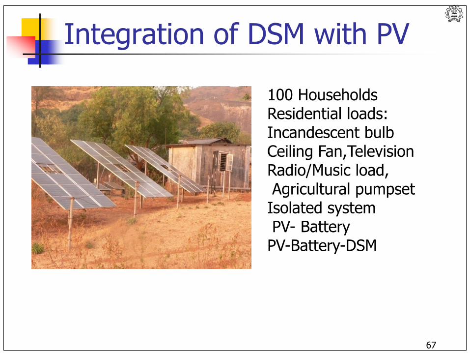
Integration of DSM with PV

67

100 HouseholdsResidential loads: Incandescent bulbCeiling Fan,TelevisionRadio/Music load,Agricultural pumpsetIsolated systemPV- BatteryPV-Battery-DSM

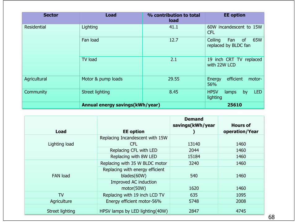
Sector Load % contribution to total load

EE option

Residential Lighting 41.1 60W incandescent to 15WCFL

Fan load 12.7 Ceiling Fan of 65Wreplaced by BLDC fan

TV load 2.1 19 inch CRT TV replacedwith 22W LCD

Agricultural Motor & pump loads 29.55 Energy efficient motor-56%

Community Street lighting 8.45 HPSV lamps by LEDlighting

Annual energy savings(kWh/year) 25610

Load EE option

Demand

savings(kWh/year

)

Hours of

operation/Year

Lighting load

Replacing Incandescent with 15W

CFL 13140 1460

Replacing CFL with LED 2044 1460

Replacing with 8W LED 15184 1460

FAN load

Replacing with 35 W BLDC motor 3240 1460

Replacing with energy efficient

blades(60W) 540 1460

Improved AC induction

motor(50W) 1620 1460

TV Replacing with 19 inch LCD TV 635 1095

Agriculture Energy efficient motor-56% 5748 2008

Street lighting HPSV lamps by LED lighting(40W) 2847 4745

68

0

5

10

15

20

25

0 1 2 3 4 5 6 7 8 9 10 11 12 13 14 15 16 17 18 19 20 21 22 23 24

Laod

of

are

a(k

W)

Time of day(h)

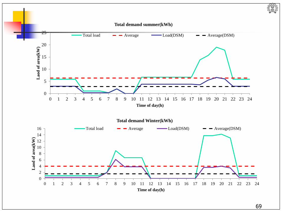
Total demand summer(kWh)

Total load Average Load(DSM) Average(DSM)

0

2

4

6

8

10

12

14

16

0 1 2 3 4 5 6 7 8 9 10 11 12 13 14 15 16 17 18 19 20 21 22 23 24

Laod

of

are

a(k

W)

Time of day(h)

Total demand Winter(kWh)

Total load Average Load(DSM) Average(DSM)

69

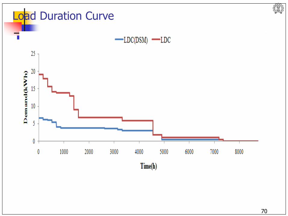
Load Duration Curve

70

EE technologies, systems

Technology Development

Research

Innovation

Grand Challenges

Market transformation

Capacity and Institution Building

71

Concluding Remarks

Redefining utility role

Load and Supply Variability

Analysis of Load profiles and consumer price elasticities

Participation rates, Transaction costs

Flexibility and Resilience in Power system

Innovation

DSM to be integrated into Energy planning

DSM in curriculum

Thank you 72

References

FERC, 2009 http://webarchive.nationalarchives.gov.uk/20121217150421/http://www.decc.gov.uk/ass

ets/decc/statistics/publications/trends/articles_issue/560-trendssep10-electricity-demand-article.pdf

Power System Statistics 2012-13, KSEB: KERALA STATE ELECTRICITY BOARD LIMITED J.K. Parikh , B.S.Reddy and R.Banerjee, Planning for Demand Side Management in the

Electricity sector, Tata McGraw Hill , New Delhi,1994. S Ashok and Rangan Banerjee, Optimal Operation of Industrial Cogeneration for Load

Management, IEEE Transactions on Power Systems, Vol 18, No. 2, May 2003. S. Ashok and Rangan Banerjee, Optimal cool storage capacity for load management,

Energy 28 (2003) 115-126. R.Banerjee, "Load management in the Indian power sector using US experience", Energy,

Vol 23, 1998 , pp 961-973 Puradbhat, S. and Banerjee, R., "Estimating Demand Side Management Impacts on

Buildings in Smart Grid." The 2014 IEEE ISGT Asia Conference on 'Innovative Smart Grid Technologies (ISGT Asia 2014), Berjaya Times Square Hotel, Kuala Lumpur, Malayasia, May 20-23, 2014.

73

[email protected]

irp and demand side management- basics - dsm -...

Documents