irwin/mcgraw-hill © andrew f. siegel, 1997 and 2000 4-1 l chapter 4 l introduction to statistical...

Irwin/McGraw-Hill © Andrew F. Siegel, 1997 and 2000

4-1

l Chapter 4 l

Introduction to Statistical Software

Package 4.1 Data Input 4.2 Data Editor 4.3 Data Computation and Transformation


4-2

n

XXXX n

...21

N

XXX N

...21

Sample average

Population average

“X-bar”

“mu”

n

iiX

nX

1

1

N

iiX

N 1

1

Introduction to Statistical Software PackageThe statistical software package used – SPSS (Statistical

Package for the Social Sciences) v. 21/v. 22Sophisticated software used by social scientists and related

professional for statistical analysis.Compatible with the Windows environment.


4-3

0

2

0 5 10 15 20Defects per lot

Fre

quen

cy (

lots

)

Average is 5.1defects per lot

4.1 Data InputDefining variables (in Variable view):

Variable names Labels (Variable and value) Missing values Variable types Column format Measurement level


4-4

5+72

4.1 Data InputVariable names

Must begin with letter. The remaining can be letter, digit, period or the symbols @, #, _ or $.

Cannot end with period or underscore Blanks and special characters cannot be used (E.g.: !, ?, ‘ and *) Must be unique; Duplication is not allowed The length in one variable cannot exceed 64 characters Reserved keywords cannot be used as variable names (E.g.: ALL,

AND, BY, EQ, GE, LE, LT, NE, NOT, OR, TO and WITH) Are not case sensitive


4-5

4.1 Data InputLabels

Variable label is a full description of the variable name Optional It has a value label that can be in alphanumeric and numeric code

Alphanumeric code

Numeric code


4-6

Ranks

Rank of median= (1+8)/2 = 4.5

0 1 2 3 4 5

3 1 8 8 56 49

Median Average

Data

4.1 Data InputMissing values

How to dealt with missing data – Leave the cell blank or assign missing value codes

Rules for assigning missing value codes: Must be the same data type as they represent (E.g.: Missing numeric data

must use numeric missing value code) Missing value code cannot occur as data in the data set By default, the choice of digit is usually 9

Variable types By default, SPSS assumes all new variables are numeric with two

decimal places. Can be changed to other type (date, currency, etc) and have different

number of decimal


4-7

0

5

-20% -10% 0%Percent change at opening

Fre

quen

cy

Average = -8.2%

Median = -8.6%

4.1 Data InputColumn format

It is possible to adjust the width of the Data Editor columns and change the alignment of data in the column (left, centre or right)

Measurement level Can be specified as nominal, ordinal, interval or ratio


4-8

0

10

20

30

40

50

$0 $100,000 $200,000 Income

Average = $38,710

Median = $27,216

Fre

quen

cy

4.2 Data EditorSpecifically, in editing and viewing data and result in SPSS,

it has seven different types of windows: Data editor (Our focus) Viewer and draft viewer (Output) Pivot table editor Chart editor Text output editor Syntax editor Script editor


4-9

Mode

Mode

4.2 Data EditorData view


4-10

Average, median, and modeare identical

in the case of a normal distribution

4.2 Data EditorVariable view


4-11

Average

Median

Mode

4.2 Data Editor


4-12

Average

Median

Mode

4.2 Data EditorToolbar

File save

File open

File print

Dialog recall

Undo

Redo

Go to case

Go to variable

Variable

Run descriptive statistics

Find

Insert cases

Insert variable

Split file

Weight cases

Select cases

Value labels

Use sets

Show all variables

Spell check


4-13

Average

Median

Mode

4.2 Data EditorExercise

Enter the following cases:


4-14

Average

Median

Mode

4.3 Data Computation and TransformationData screening

Objectives: Making sure that data have been entered correctly Making sure that the distributions are normal

The importance of data screening May affect the validity of the results that are produced May assist in deciding; the need of data transformation, the usage of

nonparametric techniquesThis subtopic will be demonstrated using data of work3.sav


4-15

Average

Median

Mode

4.3 Data Computation and TransformationErrors in data entry

Error in data entry are common and therefore data files must be carefully screened

Use Frequencies or Descriptive command Output example:


4-16

Average

Median

Mode

4.3 Data Computation and TransformationAssessing normality

The assumption of normality is prerequisite of many inferential statistical techniques

Normality can be explored using a combined assessment of graphic: Histogram Boxplot Normal probability plot Detrended normal plot

And normality test: Kolmogorov-Smirnov and Shapiro-Wilk statistics Skewness Kurtosis


4-17

Average

Median

Mode


Performed using the Explore command in Descriptive Statistics under Analyze Histogram

Need to be Bell

shaped /symmetry


4-18

Average

Median

Mode


Boxplot Median should be

at the center of the

body (symmetric)


4-19

Average

Median

Mode


Normal probability plot Plot should fall more

or less in a straight line


4-20

Average

Median

Mode


Detrended normal plot There should be no

pattern to the

clustering of points

(The point should

assemble around

a horizontal line

through zero)


4-21

Average

Median

Mode


Kolmogorov-Smirnov and Shapiro-Wilk statistics

Kolmogorov-Smirnov Sample size 100

Shapiro-Wilk Sample size < 100

If the significance level (Sig.) is greater than 0.05, normality is assumed


4-22

Average

Median

Mode


Skewness and Kurtosis Their value need to be close

to zero to be assumed normal

Basically, the data of age can be assumed normal There is no need for transformation Data can be analyzed using parametric test


4-23

Average

Median

Mode

4.3 Data Computation and TransformationVariable transformation

The decision to transform variables depends on the severity of the departure from normality

Most appropriate transformation method need to be selected*

*Suggested by Tabachnick and Fidell (2007) and Howell (2007)

C = A constant added to each score so that the smallest score is 1

K = A constant from which each score is subtracted so that the smallest score is 1; usually equal

to the largest score + 1

Data distribution Transformation method [Num. Expression]Moderately positive skewness Square-Root [SQRT(X)]

Substantially positive skewness Log 10 [LG10(X)]

Substantially positive skewness(with zero values)

Log 10 [LG10 (X + C)

Moderately negative skewness Square-Root [SQRT(K - X)]

Substantially negative skewness Log 10 [LG10(K - X)]


4-24

Average

Median

Mode








To illustrate the process of transformation, the hours of exercise (hourex) will was examined using the preceding steps.


4-25

Average

Median

Mode








It is obvious that variable hours of exercise (hourex) is not normal. Variable transformation need to be performed

Based on previous assessment, we know that variable hourex is not normally distributed but is significantly positively skewed and because of the is no zero value involved, Log 10 transformation method should be performed.


4-26

Average

Median

Mode








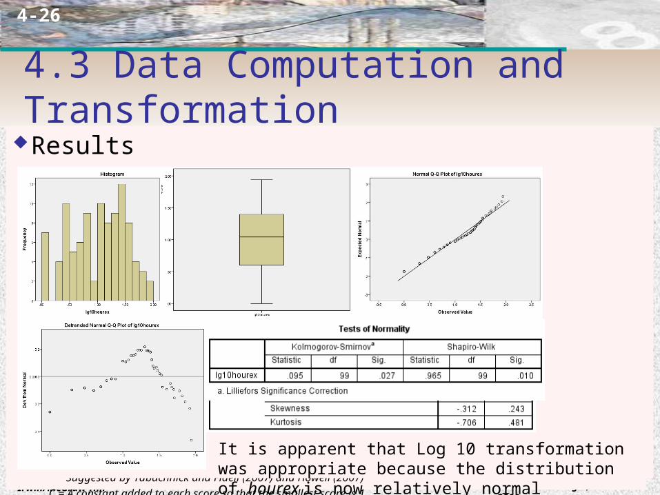
Results

It is apparent that Log 10 transformation was appropriate because the distribution of hourex is now relatively normal


4-27

Average

Median

Mode








Data transformation Recoding

Collapsing continuous variables into categorical variables Recoding negatively worded scale items Replacing missing values and bringing outlying cases into the distribution

Computing To obtain composite scores for items on a scale

Data selection In the Select Cases option in the Data menu, data can be selected:

On specified cases using If option Randomly using the Sample option Based on time or case range using the Range option

irwin/mcgraw-hill © andrew f. siegel, 1997 and 2000 4-1 l chapter 4 l introduction to statistical...

Documents