is a value added tax annual versus … is a value added tax regressive? at the peak of their age...

IS A VALUE ADDED TAX REGRESSIVE? ANNUAL VERSUS LIFETIME INCIDENCE MEASURES ERIK CASPERSEN* & GILBERT METCALF**

Abstract - We measure the lifetime incidence of a value added tax (VAT) using data from the Panel Study of Income Dy- namics (PSID) and the Consumer Expendi- ture Survey (CEX). Using annual income to measure economic well-being makes a VAT look quite regressive. Using two different measures of lifetime income, we find that a broad-based VAT would be on/y modestly regressive. Using current consumption as a proxy for lifetime income makes a VAT proportional. We discuss why these two approaches to measuring lifetime income lead to different incidence results. We also consider the distributional impact of zero rating food, housing, and medical expenditures.

INTRODUCTION

Despite its widespread use in Europe and other parts of the world, a national value added tax (VAT) has never been adopted in the United States. One concern expressed by many policymakers is

*Harvard Law School, Cambndge, MA 02138

**Department of Economics, Tufts Umverslty, Medford, MA

02155

the believed incidence of a VAT. A VAT ultimately is a tax on goods and services and thus is a tax on consumption. Con- ventional economic wisdom holds that consumption taxes are passed forward to the consumer (viz. Pechman, 1985). Poor people spend greater percentages of their annual income on consumption and thus would pay a greater percentage of their income on the VAT tax. In other words, the VAT would be regressive.’

In recent years, the perception that a VAT (as well as other consumption taxes) would be regressive has been questioned by researchers who have conducted tax incidence analyses using a consumption measure to proxy for lifetime income (e.g., Poterba, 1989, 1991; and Metcalf, 1994a). They have found considerably less regressivity of consumption taxes. In this paper, we estimate lifetime income using data from both the Consumer Expenditure Survey (CEX) and the Panel Study of Income Dynamics (PSID). The virtue of this approach is that it draws on the strengths of each data set: the PSID has rich annual income data from which measures

731

of lifetime income can be constructed, while the CEX has very good consumption data wrth which we can construct the tax base for a VAT at the household llevel. We compare measures of the distribution of a VAT using two lifetime in- (come measures drawn from the PSID to an annual income measure, as well as a measure of current consumption.

Our analysis proceeds in three stages. First, we construct income age profiles In .the PSID from which we can compute ,the present discounted value of earned income and gifts (i.e., lifetime income) for a household. The regression includes (demographic variables on the household that are common to both the PSID and the CEX. Second, we take the estimated #coefficients from this regression and apply them to households in the CEX to calculate an estimate of lifetime income. Finally, we can compute a VAT tax liability in the CEX and carry out the distributional analysis using our measure of lifetime income. We contrast the results of the analysis using this approach to measure lifetime Income to results where annual income and current consumption are used as income measures for distributional analysis.

In brief, we find that over the life cycle, a VAT looks substantially less regressive than when viewed in the context of a single year. In contrast, when current consumption is used as a proxy for lifetime income, the tax is by definition proportional. When food, housing, and medical expenditures are zero rated, the VAT looks somewhat less regressive in the lifetime income analysis. If current consumption is used to measure economic welfare, the VAT now looks mildly progressive.

We begin in the second section with a review of the relevant literature and a consideration of some of the theoretical issues involved in such an analysis. In the

third section, we proceed with the specification and estimation of a life-cycle incidence model. In Section 4, we discuss the model’s findings and conclude.

BACKGROUND

Early tax incidence studiles used the results of partial or gener I equilibrium models to inform judg d ents about relevant incidence results. In effect, these studies used existing re earth results to

x generate plausible assu ptions about the incidence of specific taxes. Pechman (1985) represents the classic example of this type of research. The time frame for analysis is one year, ano Pechman assumes that consumption taxes are passed forward and borne by consumers In proportion to their expenditures. Tak- ing this approach, Pechman finds that consumption taxes are quite regres- s1ve.2,3

An alternative approach utilizes estimates of lifetime incom’ le as a measure of the taxpaying unit’s economic well- being. Invoking Friedman’s (1957) permanent illcome hypothesis as well as life-cycle considerations, economists have recognized that annual Iincome may not be a very good measure of an individual’s potential to consume. With perfect capital markets, individuals should be grouped according to the present discounted value of earnings plus gifts received. This theory makks the difficulties with the annual incidenice approach readily apparent. People tend to earn the highest Incomes in their life around middle age and the lowest incomes in their youth and old age. Consequently, in a cross-sectional (annual) analysis, lower income groups are likely to include some young and elderly people (as well as some people w&h volatile incomes who have obtained a low realiza- tion) who are not poor’ in a lifetime sense. Similarly, higher annual income groups are likely to comain some people

732

I IS A VALUE ADDED TAX REGRESSIVE?

at the peak of their age earnings profile for whom peak earnings are a poor measure of annual ability to consume.

Relative to annual income, lifetime income is more difficult to measure. Po- terba (1989, 1991) has proposed using consumption as a proxy for lifetime income, arguing that since household consumption tends to be smoother than income, total annual consumption is likely to be a better measure of household well-being than total annual income. Us- ing data on total expenditures from the CEX, Poterba finds that excise taxes on alcohol, tobacco, and gasoline are much less regressive than they appear when viewed in an annual income framework. Metcalf (I 994a) has used a similar approach to analyze state and local tax systems. Like Poterba’s findings for excise taxes, he finds that the system of state and local taxes is less regressive when consumption is used to proxy for lifetime income.

Over the past couple of years, several economists have examined the incidence of various taxes using life-cycle models. Fullerton and Rogers (1991 and 1993) estimate lifetime income in a large scale multigeneration CGE framework. The authors first estimate age-wage profiles. Using data on individuals from the PSID, they regress the wage rate on time, the age of each individual, the age squared, the age cubed, and various demographic variables.4 The results of this regression describe how a person’s earnings potential changes over time as a consequence of age and the other factors. Once these profiles are determined, each person in the data set can be assigned a measure of his or her respective lifetime income. This is calculated by summing up the discounted values of the areas under the estimated age-wage profiles for each person.

Once individuals are categorized by the

present value of lifetime wage potential, Fullerton and Rogers (1991 and 1993) then proceed to re-estimate profiles for each group and to calculate tax incidence estimates based on the age-income profiles and the lifetime income measurements. They find that both the corporate and individual income taxes appear to be less progressive in a life- cycle framework, while sales and excise taxes appear to be less regressive. It is also noted that, despite these changes, the overall incidence of the United States tax system seems to be about the same as it has been estimated under an annual income framework.5

Fullerton and Rogers (1991 and 1993) present the most careful analysis of lifetime tax incidence to date. One com- ment should be made when comparing their results on sales and excise taxes to our results on a VAT. As the authors note, sales and excise taxes are not equivalent to a uniform consumption tax. The tax rates facing consumers (on a tax exclusive basis) in their study range from zero (housing) to 79 percent (tobacco). Much of the regressivity of sales and excise taxes is due to the fact that necessities tend to be taxed at higher rates than luxury goods.

Why do consumption taxes look less regressive under a lifetime tax incidence analysis? Consider a consumption tax in a simple annual income framework in which there are no bequests:

0 Y=C+S.

In equation 1, annual income (Y) is allo- cated between consumption (C) and saving (5). The consumption tax as a fraction of income is given by

733

where 7 is the tax rate on consumption. Assuming a consumption tax is passed forward to consumers, it is regressive (in an annual context) to the extent that the savings ratio increases with income.

Now consider a consumption tax in a lifetime tax incidence framework. With n~o bequests, lifetime income (W) will equal the present discounted value of consumption (discounted at rate p) over the individual’s life:

If the tax were applied to all consump- tuon at the same rate, the tax liability would equal 7C in any year and the present discounted value of the lifetime t,ax payments would equal

El

The average tax rate (lifetime tax/‘W) vvould simply equal the statutory rate T. The tax is proportional.

Real life is more complicated. First, bequests are typically not subject to consumption taxation. Henc:e, to the extent that bequests rise with income, we will overstate the progressivity of a consumption tax. Menc:hik and David (1982) find that the ratro of expected bequests to lifetime earnings is U shaped with the trough at the 80th percentile. This suggests that ignoring bequests will only understate the regressivity of a consumption tax for the top of the income distribution and that, in fact, over the rest of the distribution, we might be underestimating the progressivity of the tax by ignoring bequests. Second, in addition to excluding bequests from the

tax base, i3 VAT would likely tax at lower (or zero) rates ite& such as food, housing, and medical care. To the extent that these excluded itemp are necessities, a consumption tax will tend to move toward progressivlty.

Like recent researchers in this area, we propose to engage in a lifetime incidence analysis. We should note at this point that there are diffdrent “lifetime” experiments that one can analyze. As Poterba (1993) points oqt, one can look at lifetime tax burdens apd/or lifetime income. Fullerton and Rogers (1993) look at the lifetime tax burden relative to lifetime income, whereas Poterba (1989, 1991) and Metcalf (1994a, b) look at annual tax burdeins relative to lifetime income. The latter approach ad- dresses the question of the burden of a particular year’s taxes when households are classified by a measure of economic well-being that is less prbne to measure- ment error than annual income. The annual tax/lifetime income approach is taken in this paper. StricFly speaking, one cannot compare thq results from a lifetime tax/lifetime incope analysis (e.g., Fullerton and tax/lifetime income sis such as this one.

We proceed by merging income infor- rnation from the PSID with expenditure information frorn the CE~X. The next section details our construction of this measure in more detail.

SPECIFICATION AND ESTIMATION

In this section, we sketch out the model with which we estimate lifetime income. Lifetime income (W) can1 be computed either as the present discounted value of the stream of inheritances (and gifts) received (13 plus earned inFome and transfers (EJ or as the presenIt discounted value of consumption (C,) and bequests made (B,):


Ct + 4 &p2LL~~~ (1 + p)’ (1 + p)’

where p is the individual’s after tax rate of return. We will construct a measure of lifetime income from the sources side. That is, we will estimate the stream of earned income and inheritances for households and compute the present discounted value of this stream.

We proceed by estimating the relationship between age and earned income in a longitudinal data set and then use this information to generate lifetime income estimates in a cross-sectional data set. There are two steps to the procedure. First, we use the PSID to estimate age- income profiles for households. Coeffi- cient estimates from these regressions are then applied to households in the CEX to generate estimates of lifetime income for these households. For the two- step procedure, we begin by regressing the log of annual earned income plus transfers and gifts received on age, age squared, and various demographic variables. These right-hand-side variables are selected to correspond to information that is also available in the CEX.

One immediate complication arises from the possible existence of correlated individual effects when combining information from the PSID and CEX. There is a long literature on the importance of individual effects in wage regressions (see Griliches (1977) for a discussion of this literature). Unobserved ability is typically invoked as the rationale for individual effects. It is presumed that ability is correlated with education (among other things) and that omitting some measure of ability leads to biased coefficient estimates. This suggests that our income regression should include an individual (fixed) effect. While it is possible to estimate fixed effects in the PSID regression,

it is not possible to attribute those fixed effects to particular households in the CEX. Ignoring the individual effects is problematic for two reasons: (1) if these individual effects are correlated with ex- planatory variables, the coefficient estimates from a regression without fixed effects will be biased and inconsistent; and (2) we will miss important variation in lifetime income resulting from cross- sectional variation in the individual effects.

Constructing unbiased estimates of the coefficient vector is straightforward, as we can compute fixed effects estimates in the PSID. Unfortunately, all time- invariant information is lost, as these coefficient esttmates are not separately identified from the fixed effects. We can preserve some information from these variables by interacting them with age and age squared, but significant information is lost when individual effects are estimated. Moreover, there is no way to recover the fixed effects when moving from the PSID to the CEX. Thus, we face a dilemma: we can ignore the possibility of correlated fixed effects and compute coefficient estimates that may be inconsistent, or we can construct consistent coefficient estimates for all but the time- invariant variables and lose all the information contained in those variables.

The appropriate resolution of this dilemma depends on one’s loss function (i.e., one’s concerns about bias versus variance). To test the sensitivity of our distributional results to the inclusion or exclusion of fixed effects, we proceed by presenting two sets of results. The first set is based on a prediction of lifetime income in the PSID from an income regression in which fixed effects are not estimated. Thus, all time-invariant variables (education, race, etc.) can be included in the regression. These estimates will be biased in the presence of correlated fixed effects. However, more infor-

735

mation is available (the time-invariant variables), which will reduce the variance. The second set of results is based on a PSID regression in which we estimate the fixed effects. Hence, the coefficient estimates are consistent but less efficient. We then apply these coefficient estimates to CEX data and compute a Iproxy for the fixed effect in the CEX. 13elow we discuss our proxy for the fixed effect .6

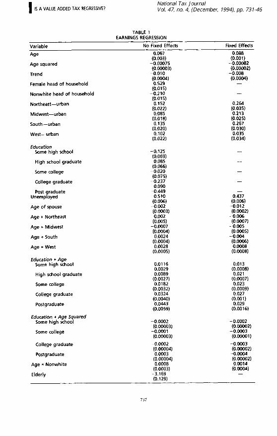
Table 1 presents regression results for our income measure.7 The regression in column 1 does not estimate the fixed effects and thus incorporates all time-invariant information in the PSID data. This regression indicates that income initially rises with age and then falls in later years. Later cohorts have lower incomes (roughly one percent per year) holding other variables constant. Residents of urban areas have higher incomes with a Iparticularly lhigher level in the west. At age 30, college graduates earn roughly ‘$5,500 more income than household lheads with a high school diploma. The (differential wrdens at age 40, with col- liege graduates earning over $12,000 /more than high school graduates (in 1980 dollars). Nonwhite and female- iheaded households earn less than white imale-headed households. The regression fits reasonably well with an R2 of 0.34.

‘The second column in Table 1 presents (coefficient estimates from a regression in Iwhich the flxed effects are estimated. ‘Thus, all time-invariant variables are (dropped.* The differences in the fixed #effects regression results are subtle but important.g Income increases more quickly with age at first but falls off more sharply in later years than in the levels regression. The regional effects are stronger for all parts of the country ex- cept the West, and the interaction variable between age (and education is now stronger. The variable measuring the interaction of age with a dummy for

being elderly now is weaker by a factor of 6 but continues to be statistically significant.

We next Iuse the regression results to estimate lifetime income in the 1988 CEX.” Lifetime income js defined here as the present discounted value of earned income, transfers, and gifts received by a given family~ over the adult life of the household head and depends only on the demographjc variables associated with each family. Our measure assumes that the individu$‘s discount rate rematns constant at four percent over time and that a household exists as an income-generating entit

Y from the time

the head is 21 until the time the head is 80. Workers are continually employed until age 65 at which point they retire. For each family, lifetime income is computed as

wherle ?,, is the fitted value of earned Income plus transfers and inheritances received for household i in year t from the appropriate regression in Table 1.

In forecasting income inI the CEX, we would like to eliminate andomness in the income measure, w 6 ich is due to annual temporary income fluctuations, while maintaining the s ochastrc ele- ments of income that a feet variance

I and skew in a persisten way.” We make an adjustment to Iour measure of lifetime income as characterized in equation 6 to account for thle loss of skew by allowing for shocks 40 income that are persistent over time We assume an AR( 1) process for a ran d om shock to log Income with first-order autocorrelation of 0.85 and variance oft the innovation of 0.05.” This will add bkew to the distribution of lifetime income.

736


TABLE 1 EARNINGS REGRESSION

Variable

Age

Age squared

Trend

Female head of household

Nonwhite head of household

Northeast-urban

Midwest-urban

No Fixed Effects

0.067 (0.003)

-0.00075 (0.00003)

-0.010 (0.0004)

-0.529 (0.015)

-0.210 (0.015) 0.152

Fixed Effects

0.088 (0.001)

-0.00082 (0.00002)

-0.008 (0.0004)

-

-

0.264

South-urban

West-urban

Education Some high school

High school graduate

Some college

College graduate

Post raduate 9 Unemp oyed

Age of spouse

Age * Northeast

Age * Midwest

Age * South

Age * West

Education * Age Some high school

High school graduate

Some college

College graduate

Postgraduate

Education * Age Squared Some high school

Some college

College graduate

Postgraduate

Age * Nonwhite

Elderly

-0.125 (0.069) 0.085

(0.066) -0.020 (0.075)

-0.237 0.090

-0.449 -0.510 (0.006)

-0.002 (0.0003) 0.002

(0.005) -0.0007 ‘yg”4’

(0:0004) 0.0028

(0.0005)

0.0116 0.0029 0.0089

‘00.~~~;’

‘;:g;g’

(0:0040) 0.0443

(0.0059)

-0.0002 (0.00003)

-0.0001 (0.00003)

-0.0002 ’ yg’

c~:~Oo~s,

(0:0003) -3.169 (0.129)

-

-

-

-

0.437 (0.006)

-0.012 (0.0002)

- 0.006 (0.0007)

-0.005 (0.0005)

-0.004 ‘go;;’

(0:OOOB)

0.013

-0.0002 (0.00002)

-0.0003 (0.00001)

-0.0003 (0.00002)

-0.0004

‘KiE2’ (0:0004)

-

737

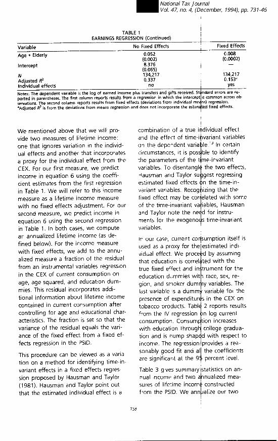
TABLE 1 EARNINGS REGRESSION (Continued) _--- -- --

iariable No Fixed Effects Fixed Effects - ;4ge * Elderly

-- 0.052 0.008

(0.0002) lhtercept -

N 134,217 134,217 Adjusted R* 0.337 0.153a llndividual effects no yes -- --

“Adjusted 2 is from the deviations from means regression and does not incorporate the estim ed fixed effects.

We mentioned above that we will provide two measures of lifetime income: one that ignores variation in the nndivid- ual effects and another that incorporates a proxy for the individual effect from the CEX. For our first measure, we predict income in equation1 6 using the coefficient estimates frorn the first regression in Table 1. We will refer to this income Imeasure as a lifetime income measure with no fixed effects adjustment. For our second measure, we predict income in equation 6 using the second regression In Table 1. In both cases, we compute #an annualized lifetime income (as de- ,fined below). For the income measure with fixed effects, we add to the annualized measure a fraction of the residual from an instrumental variables regression in the CEX of current consumption on age, age squared, and education dummies. This residual incorporates additional information about lifetime income contained in current consumption after controlling for age and educational characteristics. The fraction is set so that the variance of the residual equals the variance of the fixed effect from a fixed effects regression in the PSID.

This procedure can be viewed as a variation on a method for identifying time-invariant effects in a fixed effects regression proposed by Hausman and Taylor (1981). Hausman and Taylor point out that the estimated individual effect is a

combination of a true itidividual effect and the effect of time-invariant variables on the dependent varia circumstances, it is poss ble to identify ‘p

le.13 In certain

the parameters of the time-invariant variables. To disentanglq the two effects, Hausman and Taylor su estimated fixed effects 8

gest regressing n the time-in-

variant variables. Recogbizing that the fixed effect may be corttelated with some of the time-invariant variables, Hausman and Taylor note the neqd for instruments for the exogenods time-invariant variables.

In our Case, current colsumption itself is used as a proxy for the~estimated individual effect. We proce’ d

,’ by assuming

that education is carrel ted with the true fixed effect and initrument for the educe&ion dummies wit/7 race, sex, region, ancl smoker dumr#y variables. The last variable is a dummy variable for the presence of expenditur+ in the CEX on tobacco products. Tab@ 2 reports results from the IV regression Qn log current consumption. Consump/tion increases with education through1 college gradua- tion and is hump shapdd with respect to income. The regression provides a reasonably good fit and al

4 the coefficients

are significant at the 9 percent level.

Table 3 gives summary :statistics on annual income and two alnnualized measures of lifetime incorn+ constructed from the PSID. We annualize our two

738


TABLE 2 INSTRUMENTAL VARIABLES REGRESSION ON

CONSUMPTION FROM THE CEX

Variable

Education Dummy Some college

College graduate

Postgraduate

Age

Age squared

Intercept

Number of observations Standard error

1,506 0.661

Notes: The dependent variable is the log of current consumption. Instruments include race and sex of household head, region in which household resides, and whether a member of the household smokes. Standard errors are reported in parentheses.

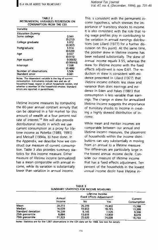
lifetime income measures by computing the 60-year annual constant annuity that can be obtained in a fair market for this amount of wealth at a four percent real rate of interest.14 We will also provide distributional results in which we use current consumption as a proxy for lifetime income as Poterba (1989, 1991) and Metcalf (1994a, b) have done. In the Appendix, we describe how we construct our measure of current consumption. Table 3 also provides summary statistics for this income measure. Either measure of lifetime income (annualized) has a mean comparable with annual income, while its variation is substantially lower than variation in annual income.

This is consistent with the permanent income hypothesis, which stresses the importance of transitory shocks to income. It is also consistent with the role that rising wage profiles play in contributing to the variation in annual earnings distribu- tions (see Lillard (1977) for a further discussion on this point). At the same time, the positive skew in lifetime income has been reduced substantially. The skew of annual income equals 3.55, whereas the skew for lifetime income with the fixed effects adjustment is now 0.61. The re- duction in skew is consistent with evidence presented in Lillard (1977) that lifetime income exhibits less skew and variance than does earnings and evidence in Eden and Pakes (1981) that consumption is less variable than earnings. The change in skew for annualized lifetime income suggests the importance of transitory shocks to income in creat- ing a highly skewed distribution of income.

While mean and median incomes are comparable between our annual and lifetime income measures, the placement of households within the income distri- butions can vary substantially in moving from an annual to a lifetime measure. The differences are particularly large in the lowest annual income decile. Con- sider our measure of lifetime income that has a fixed effects adjustment. Ten percent of the households in the lowest annual income decile have lifetime in-

TABLE 3 SUMMARY STATISTICS FOR INCOME MEASURES

Lifetime Income

Annual Fixed Effects Adjustment? Current

Income No Yes

Mean 20,273 20,219 Median 19,402 16,620 19,653 Standard deviation 18,765 16,230 8,145 25th percentile 7,526 8,884 13,616 75th percentile 13,800 27,323 25,620

24,008 Notes: Statistics are for the 1,507 observations in the CEX data set for 1988. See text for details,

Consumption

15,268 13,398 9,348 8,670

19,733

739

(come above the median Almost 20 per- (cent of the households in the second (annual income decile have lifetime in- (come above the median

DISTRIBUTIONAL IMPACT OF A VAT

‘We now turn to measuring the distributional impact of a .five percent VAT. Be- fore turning to the results, we briefly discuss some of the basic assumptrons behind the analysis. We begin by noting that we are conducting an absolute incidence analysis. Thait is to say, a VAT is introduced without the removal or alter- ation of any existing forms of taxation. Furthermore, we assume that government expenditures would not change in size or composition with the introduction of a VAT.” Second, we assume that the VAT is passed forward to consumers. Consequently, the amount of tax burden falling on a consumer unit is the statutory rate multiplied by the dollar amount of consumption. This assumption accords with previous work measuring the incidence of consumption taxes (e.g., Pech- man, 1985; Musgrave, Case, and Leon- ard, 1974). It can be justified by assuming that the supply of consumption goods is perfectly elastic, as would be the case with perfectly competitive markets and constant returns to scale in production. The additional virtue of this assumption is that we can easily compare our findings about the incidence of a VAT with findings of previous researchers who have looked at consumption taxes. Third, we take as the unit of observation the household, arguing that major consumption decisions are typically made at the household level.

The tax base for the VAT in the absence of any zero-rated goods is current consumption (as defined in the Appendix). Thus, we are assurning that expenditures that are forms of saving (e.g., contribu- tions to pension plans) are not included in the tax base. Moreover, the VAT taxes

durables <as they are consumed.16 We will consider two different VAT struc- tures. In the first, all consumption is taxed, and in the second, food, housing, and health expenditures are zero rated.

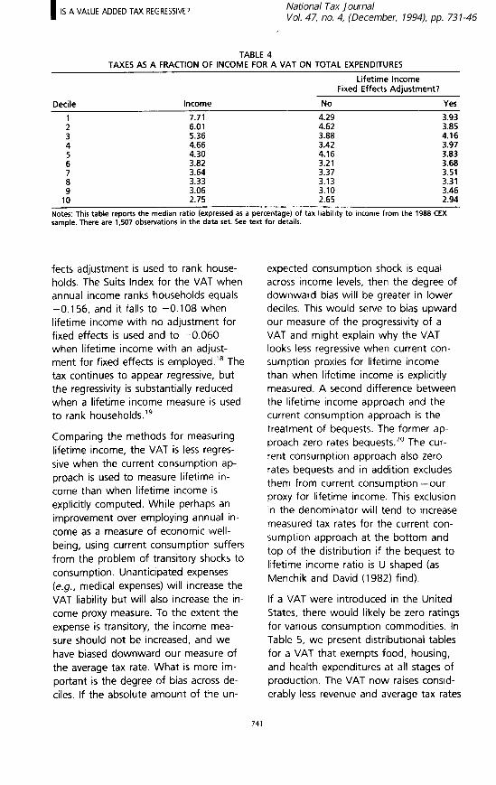
We compute average tax rates for each household by dividing the household’s tax liability by the relevant measure of Income. Table 4 shows the median tax rate for each decile under three different measures of income for a VAT applied to all consumption. When annual income is used as a measure of economic well-being, the VAT is clearly regressive. The rnedian tax rate for the lowest de- tile is 7.7 percent and falls to 2.8 percent in the top decile. The rates fall monotomcally with income across the deciles. This result is fairly typical of analyses looking at con$umption taxes relative to annual income.17

Shifting to the lifetime perspective, the regressivity of the tax is significantly blunted. lln column 2 of Table 4, we turn to a lifetime incomie measure based on the income regression in the PSID with no adjustment for ~fixed effects. The tax is substantially less regressive with average tax rates now falling from 4.3 percent in the lowest decile to 2.6 percent in the top decile. Rates no longer fall monotonically with income. When we move to the measure of lifetime income with an adjustment for fixed effects, the tax becomes even less regressive. The rate in the lowest decile is now 3.9 percent and falls to 2.9 percent in the top decile. Again, there is no pattern of falling or rising rates across the income deciles.

Whereas the ratio of the tax rates in the first to the tenth deciles equals 2.8 when annual income is used to rank households, the ratio drops to 1.6 when the lifetime income measure with no fixed effects is used and to 1.3 when the lifetime measure with the fixed ef-

740


TABLE 4 TAXES AS A FRACTION OF INCOME FOR A VAT ON TOTAL EXPENDITURES

Lifetime Income Fixed Effects Adjustment?

Decile Income No Yes

1 7.71 4.29 3.93 2 6.01 4.62 3.85 3 5.36 3.88 4.16 4 4.66 3.42 3.97

2 4.30 3.82 4.16 3.21 3.83 3.68

2: 3.64 3.33 3.37 3.13 3.51 3.31 9 3.06 3.10 3.46

10 2.75 2.65 2.94

Notes: This table reports the median ratio (expressed as a percentage) of tax liability to income from the 1988 CEX sample. There are 1,507 observations in the data set. See text for details.

fects adjustment is used to rank households. The Suits Index for the VAT when annual income ranks households equals -0.156, and it falls to -0.108 when lifetime income with no adjustment for fixed effects is used and to -0.060 when lifetime income with an adjustment for fixed effects is employed.” The tax continues to appear regressive, but the regressivity is substantially reduced when a lifetime income measure is used to rank households.‘g

Comparing the methods for measuring lifetime income, the VAT is less regressive when the current consumption approach is used to measure lifetime income than when lifetime income is explicitly computed. While perhaps an improvement over employing annual income as a measure of economic well- being, using current consumption suffers from the problem of transitory shocks to consumption. Unanticipated expenses (e.g., medical expenses) will increase the VAT liability but will also increase the income proxy measure. To the extent the expense is transitory, the income measure should not be increased, and we have biased downward our measure of the average tax rate. What is more important is the degree of bias across de- tiles. If the absolute amount of the un-

expected consumption shock is equal across income levels, then the degree of downward bias will be greater in lower deciles. This would serve to bias upward our measure of the progressivity of a VAT and might explain why the VAT looks less regressive when current consumption proxies for lifetime income than when lifetime income is explicitly measured. A second difference between the lifetime income approach and the current consumption approach is the treatment of bequests. The former approach zero rates bequests.20 The current consumption approach also zero rates bequests and in addition excludes them from current consumption-our proxy for lifetime income. This exclusion in the denominator will tend to increase measured tax rates for the current consumption approach at the bottom and top of the distribution if the bequest to lifetime income ratio is U shaped (as Menchik and David (1982) find).

If a VAT were introduced in the United States, there would likely be zero ratings for various consumption commodities. In Table 5, we present distributional tables for a VAT that exempts food, housing, and health expenditures at all stages of production. The VAT now raises considerably less revenue and average tax rates

741

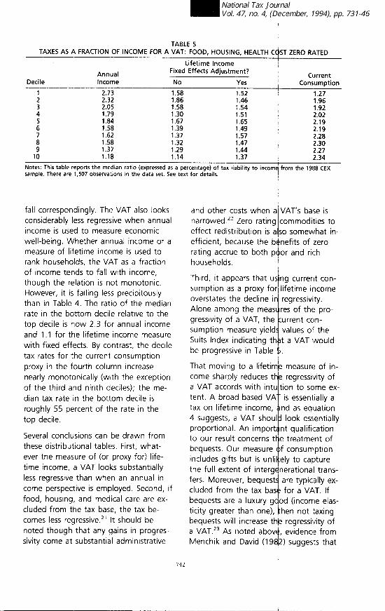
TABLE 5 TAXES AS A FRACTION OF INCOME FOR A VAT: FOOD, HOUSING, HEALTH COST ZERO RATED

Lifetime Income

Decile Annual Income --~~

Fixed Effects Adjustment? P-w

No Yes Current

Consumption

2.73 1.58 1.52 1.27 2.32 1.86 1.46 1.96 2.05 1.58 1.54 1.92 1.79 1.30 1.51 2.02 1.84 1.67 1.65 2.19 1.58 1.39 1.49 2.19 1.62 1.37 1.57 2.28 1.58 1.32 1.47 2.30 1.37 1.29 1.44 2.27 1.18 1.14 1.37 2.34

kotes: This table reports the median ratio (expressed as a percentage) of tax liability to incorny from the 1988 CEX sample. There ale 1,507 observations in the data set. See text for details.

.fall correspondingly. The VAT also looks considerably less regressive when annual income is used to rneasure economic well-being. Whether annual income or a measure of lifetime income is used to rank households, the VAT as a fraction of income tends to fall with income, though the relation is not monotonic. However, it is falling less precipitously than in Table 4. The ratio of the median rate in the bottom decile relative to the top decile is now 2 3 for annual income and 1 .l for the lifetime income measure with fixed effects. E3y contrast, the decile tax rates for the current consumption proxy in the fourth column increase nearly monotonically (with the exception of the third and ninth deciles); the median tax rate in the bottom decile is roughly 55 percent of the rate in the top decile.

Several conclusions can be drawn from these distributional tables. First, what- ever the measure of (or proxy for) lifetime income, a VAT looks substantially Less regressive than when an annual in- c:ome perspective is employed. Second, if food, housing, and medical care are ex- c:luded from the tax base, the tax be- c:omes less regressive.*’ It should be noted though that any gains in progressivity come at substantial administrative

and other costs when a~VAT’s base is narrowed.** Zero rating ~commodities to effect redistribution is also somewhat in- efficient, because the benefits of zero rating accrue to both p@or and rich households.

Third, it appears that us ng current con- i sumption as a proxy for1 lifetime income overstates the decline in regressivity. Alone among the meas u res of the progressivity of a VAT, the /current consumption measure yield4 values of the Suits Index indicating thbt a VAT would be progressive in Table 5.

That moving to a lifetim~e measure of income sharply reduces thee regressivity of a VAT accords with intu tion to some extent. A broad-based VA -c is essentially a tax on lifetime income, and as equation 4 suggests, a VAT shoul look essentially proportional. An import ! nt qualification to our result concerns tl-je treatment of bequests. Our measure of consumption includes gifts but is unlikely to capture the full extent of intergenerational transfers. Moreover, bequests are typically excluded from the tax bas e for a VAT. If bequests are a luxury gqod (income elasticity greater than one), ithen not taxing bequests will increase thle regressivity of a VAT.23 As noted abovq, evidence from Menchik and David (19q2) suggests that

742


the bequest to income ratio initially de- creases with lifetime income and only begins to increase in about the 80th percentile, and thus, the exclusion of bequests from the tax base does not have an unambiguous effect on the tax’s regressivity. However, the propensity to give bequests rises rapidly in the top quintile of income. This may explain the drop-off in average tax rates for the top decile and contribute to the regressivity of the tax in Table 4.

If bequest behavior explains the continued regressivity of a VAT in a lifetime context, new questions are raised about interpreting the results. The ultimate incidence of a VAT may depend on the underlying motivation for bequests. On the one hand, if bequest behavior is mo- tivated by strategic considerations (e.g., Bernheim, Shleifer, and Summers, 1985>, one could argue that the bequests are payments for untaxed services from potential beneficiaries. In this case, bequests should be included in the tax base and their omission will affect the overall incidence of the tax depending on the income elasticity of bequests. On the other hand, if altruistic considerations motivate bequest behavior (e.g., Blinder, 1974), one could argue that the bequest is implicitly taxed since the pur- chasing power of beneficiaries is reduced in the presence of a VAT. In this case, equation 4 can be modified so that lifetime consumption (including any bequests given) is taxed at a flat rate and the tax is exactly proportional in a lifetime context.24

Conclusions

In this paper, we have shown that when viewed from a lifetime perspective, a VAT in the United States would be substantially less regressive than when viewed in a traditional, annual income- based framework. These incidence results were generated through a two-

stage process. The first stage was the estimation of the relationship between annual income and age using longitudinal PSID data to construct a measure of lifetime income, and the second involved using this information to analyze consumption patterns with the CEX cross- sectional data set. The use of two data sets was necessary due to the lack of appropriate expenditure data in the panel data set used in the first stage.

An implicit assumption throughout this analysis has been that there are no liquidity constraints preventing households from shifting consumption forward or backward in time to match any given lifetime income profile. While this is perhaps an unreasonable assumption for a significant subset of the population, the assumption implied by annual income burden analyses that there is no consumption shifting at all is equally unreasonable. One way to think about the results in this paper is to imagine an economy scaled by its degree of liquidity constraint measured along a continuum from complete illiquidity to complete liquidity. Annual incidence analyses assume the economy is at the completely illiquid end of the continuum, while the analysis here assumes we are at the op- posite end of the continuum. Truth is probably somewhere in between. Under- standing the distributional implications of a VAT at both ends of the continuum will improve our understanding of the true burden of a VAT. In a sense, policymakers can apply a weighted average of the results from the two types of studies to draw conclusions about the ultimate distributional impact of a VAT in the United States. The weights used should depend upon the importance of liquidity constraints in limiting inter-temporal trade-offs.

This perspective suggests that the findings of this paper are of practical importance. As a result of annual income-

743

Ibased tax incidence analyses, expenditure-based taxes such as a VAT are gen- erally viewed as being fairly regressive. Consequently, some legislators have been unwilling to c:onsider implementing a VAT. Our analysis shows, however, that a VAT would be only moderately regressive over the life cycle. Moreover, adjustments such as zero rating would be effective at further reducing a VAT’s regressivity. With regressivity less of a le- gitimate concern, the political feasibility of a VAT might be enhanced.

ENDNOTES

Norman Thtirston has provided excellent research assistance on this project. The authors thank Alan Auerbach, Don Fullerton, Harvey Rosen, Jon Skinner, and Joel Slemrod for valu- able comments.

’ Conservatives are also suspicious of a VAT arguing that ;t is a “hidden” tax and will act as a money machine for the federal government, driving up revenues and hence expenditures. We do not deal with this argument in our paper. For evildence on this point, see Stockfisch (1985).

’ Variants on the annual approach abound. Musgrave, Case, and Leonard (1974) arrive at similar conclusions. Brashares, Speyrer, and Carlson (1988) analyze a VAT using an annual income measure that adds pension income less pension accruals. They too find the VAT to be substantially regressive. Ballard, Scholz, and Shoven (1987) use a CGE model to estimate the incidence (associated with the introduction of (3 VAT in the United States economy. They find the VAT to be regressive when introduced as a partial substitute for the individual income tax.

3 Browning and Johnson (1979) is an exception to the prevailrng view of this time that a VAT would be regressive Assuming that transfer programs for the poor are indexed to the price level, Browning and Johnson argue that a VAT would be a tax on factor incomes. Since the poor would be insulated from the VAT through indexing, the authors conclude that a VAT would be progressive. Methodo- logically, Browning (1985) argues that a strict differential Incidence analysis must hold all expenditures (including transfers) constant. Thus, whether real AFDC Ibenefits are held constant in actuality is not relevant. To allocate a VAT to consumption, one strictly speaking should

consider a composite pro ram change in which a VAT is levied an

I

transfers are held constant in norninal term

4 The wage rate is used he e as a measure of annual endowment so th t leisure and the utility associated with it cbn be incorporated into the model

” Lyon and Schwab (1991) Iuse a sirnilar approach to estimate the intidence of excise taxes on alcohol and tobqcco. They find little difference between the apnual and lifetime approachs for cigarettes ut find alcohol taxes to be substantially less re 1 ressive In the life- cycle analysis.

” We also have constructed measures of lifetime income in which we use the coefficients of the fixed effects regre ,sIon J in the PSID and do not estimate fixed eff

e cts for the CEX households. While the distribution of lifetime income thus measured is blightly different than the distribution whele we compute CEX fixed effects, the basic results remain un- changed.

’ In our context, income is defined as earned Income plus all cash tran

t ers. Transfers in-

clude public transfers (e.g., AFDC and Social Security payments) plus plivate transfers (gifts received).

8Note that we can Identify unemployment sta- tus and region dummies ip this regression, as there is ,variation within hbuseholds over time for these variables.

’ We test for the presence iof correlated fixed effects with a Hausman specification test. The test statistic is chi-square with 24 degrees of freedom and equals 1,891. We easily reject the hypothesis of no corrqlated fixed effects. This precludes the use of a random effects es- timator (3s a way to circurpvent estimating fixed effl?cts in the CEX.

” The CEX IS a cross-sectio 1 ‘al study that has

been conducted annually ince 1980. The data set is made up of t

I

o parts, a quarterly interview and a two-wee diary, whic:h provide detailed expenditure information for over 5,000 families. We use d ta from the quarterly interviews, as they i

j

elude some important expendttures (e.g., a tomobiles and other durables) that are not co\/lered by the diaries. All monetary figures in th PSID and CEX are converted into 1982 dollars. e

” There is considerable evid’ rice of skew in the distrrbutlon of income (e. ., Lillard, 1977). Large positive skew indicates outliers with large income. If consump ion is less skewed than income, income ske i will drive down average tax burdens in the top decile.

” There is substantial evideqce of large uncer-

744


13

14

15

16

17

18

19

20

21

22

23

24

tainty in earned income (e.g., Abowd and Card, 1979), as well as high persistence in shocks to earnings (e.g., Parsons, 1978). Our parameter choices follow those of Engen and Gale (1993). Another way to think of the estimated individual effect is that it is the combination of unobservable individual characteristics (e.g., taste, ability) and observable characteristics (e.g., education). The annual equivalent (V) is given by the for- mula Y = [l /p - 1 /p(l + p)‘], where p is the interest rate and T the length of contract. We ignore the distributional effects of changes in the deficit. In practice, durables would be taxed (if at all) on a tax prepayment basis. See Bradford (1986) for a discussion of the treatment of durable goods under consumption taxation. For example, Pechman (1985, Table 4-l 0, p. 58) reports tax rates for sales and excise taxes falling from 8.4 percent in the lowest decile to 2.1 percent in the highest decile. The Suits Index is a tax-based analogue to the Gini Coefficient. It ranges from -1 to 1 with negative values indicating a regressive tax and positive values a progressive tax. If we rank households by current consumption, the average tax rate by construction will equal 5 percent for all households and the Suits Index for the tax will equal zero. Note, though, that our measure of lifetime income is unaffected by the treatment of bequests, since we measure lifetime income on the sources side. The Suits Index for the four income measures in Table 5 is -0.143, -0.105, -0.034, and 0.035, respectively. See McLure (1993) for a discussion of this point. One alternative to increase a VAT’s progressivity that avoids the administrative costs arising from zero rating items is to im- plement a broad-based VAT with a fixed re- fundable household credit. Such a proposal is analyzed by Metcalf (1994b). The ratio of bequests to income increases with income if and only if the income elasticity of bequests exceeds one. We ignore the possibility of a VAT being temporary or the rate being changed over time, complications that are beyond the scope of this paper.

REFERENCES

Abowd, John and David Card. “On the Co- variance Structure of Earnings and Hours Changes.” Econometrica 57 (1989): 41 l-46.

Ballard, Charles L., J. Karl Scholz, and John B. Shoven. “The Value Added Tax: A General Equilibrium Look at Its Efficiency and Incidence.” In The Effects of Taxation on Capital Accumula- tion, edited by Martin Feldstein, 445-74. Cam- bridge, MA: National Bureau of Economic Re- search, 1987. Bernheim, Douglas, Andrei Shleifer, and Lawrence Summers. “The Strategic Bequest Motive.” Journal of Political Economy 93 (1985): 1045-76. Blinder, Alan. Toward an Economic Theory of income Distribution, Cambridge, MA: MIT Press, 1974. Bradford, David. Untangling the Income Tax, Cambndge, MA: Harvard University Press, 1986. Brashares, Edith, Janet Speyrer, and George Carlson. “Distributional Aspects of a Federal Value-Added Tax.” National Tax Journal 4 1 (1988): 155-74. Browning, Edgar. “Tax Incidence, Indirect Taxes, and Transfers.” National Tax Journal 38 (1985): 525-33. Browning, Edgar and William Johnson. The Distribution of the Tax Burden, Washington, D.C.: American Enterprise Institute, 1979. Cutler, David and Lawrence Katz. “Macroeco- nomic Performance and the Disadvantaged.” Brooklngs Papers on Economic Activity 2 (199 1) : 1-61. Eden, Benjamin and Ariel Pakes. “On Measur- ing the Variance-Age Profile of Lifetime Earn- ings.” Review of Economic Studies 48 (1981): 385-94. Engen, Eric and William Gale. 1993. IRAs and Saving in a Stochastic Life-Cycle Model. Brook- ings. Mimeo. Friedman, Milton. A Theory of Consumption Function, Princeton, NJ: Princeton University Press, 1957. Fullerton, Donald and Diane L. Rogers. “Life- time versus Annual Perspectives on Tax Inci- dence.” National Tax Journal 44 (1991) 277-87. Fullerton, Donald and Diane L. Rogers. Who Bears the Income Tax Burden? Washington, D.C.: Brookings Institution, 1993. Griliches, Zvi. “Estimating the Returns to Schooling: Some Econometric Problems.” Econo- metrica 45 (1977): l-22. Hausman, Jerry and William Taylor. “Panel Data and Unobservable Individual Effects.” Econ- ometnca 49 (1981): 1377-98. Lillard, Lee. “Inequality: Earnings vs. Human Wealth.” American Economic Review 67 (1977): 42-53. Lyon, Andrew B. and Robert M. Schwab.

745

1991. “Consumption l-axes in a Life-Cycle Framework: Are Sin Taxes Regressive?” Working Paper No. 3932. Cambridge, MA: National Bu- reau of Economic Research. McLure, Charles. “Economic, Administrative, and Policy Factors in Choostng a General Con- sumption Tax.” National Tax Journal 46 (1993): 34558. Menchik, Paul and Martin David. “The Inci- dence of a Lifetime Consumption Tax.” National Tax Journal 35 (I 982): 189-,203.

Metcalf, Gilbert. The Lifetime Incidence of State and Local Taxes: Measuring Changes During the 1980's. In Tax Progressivity and Income Inequal- ity, edited by Joel Slemrod, 59-88. New York: Cambridge University Press, 1994a. Metcalf, Gilbert. “Lifecycle vs. Annual Perspec- tives on the lncldence of a Value Added Tax.” Tax Policy and the Economy ,B (199413): 45-64. Musgrave, Richard, Karl Case, and Herman Leonard. “The Distribution of Fiscal Burdens and Benefits.” Public F/nance Quarter/y 2 (1974): 259~-31 I.

Parsons, Donald. “The Autocorrelatron of Earn- ings, Human Wealth Inequality, and Income Con- tingent Loans I’ Quarter/y Journal of Economic5 92 (1978): 551 -69.

Pechman, Joseph A. Who Bears the Tax Bur- den? Washington, D.C..: Brookings Institution, 198s. Poterba, James M. “Lifetirne Incidence and the Distributional Burden of Excise Taxes.” American Economic Review 79 (2) (1989): 325-30

Poterba, James M. “Is the Gasoline Tax Regres- sive?” In Tax Policy and the Economy 5 (199 1). 145-64.

Poterba, James M. Review Iof “Who Bears the Lifettme Tax Burden?” National Tax Journal 44 (4) (1993): 539-42.

Stockfisch, Jacob. “Value-Added Taxes and the Size of Government: Some Evidence.” National Tax Journal 38 (1985): 547-52.

APPENDIX: A CONSUMPTION PROXY FOR LIFETIME

INCOME

We begin by constructing a measure of current consumption as a proxy for ltfetirne income using data from the CEX. This approach operates from the assumption that consumption IS relatively smooth over the ltfe cycle. Current clbnsumption is defined as total expenditures less new vehicle purchases and housing costs for homeowners plus the imputed rental values for housing (for homeowners) and au- tomobiles In addition, we net out contributrons to

Variable ~----

I Coefficient Estimate

~- Age

Expenditures on other goods

Expenditures squared (x 1000)

Income

Family size

Female

Nonwhite

Intercept N R2

I -2.83

I "y;'

(0:02) -0.0016 (0.0023)

-0.07 (0.01)

-397.29 (98.36)

482.66 I (335.45)

947.22 (609.98)

I -1,131.99 (2,252.85)

408 0.557

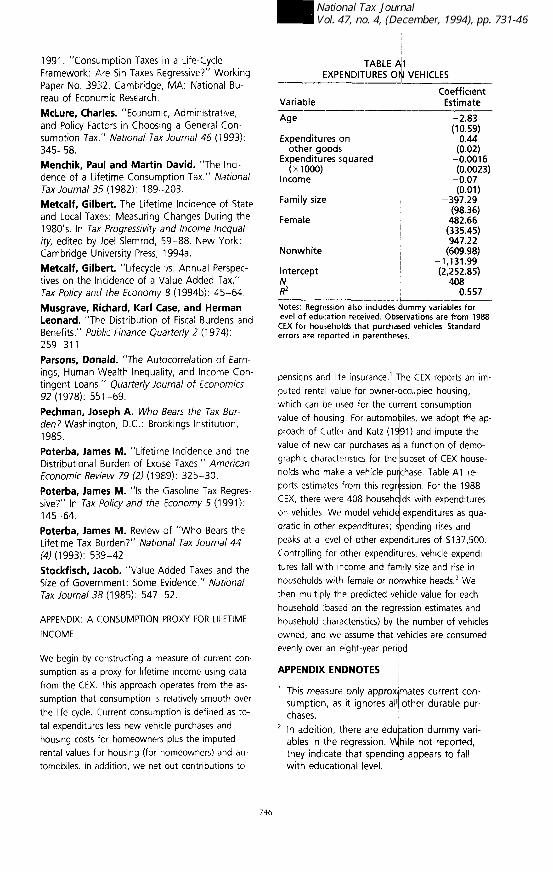
Notes: Regression also includes ummy variables for level of education received. Obs rvations are from 1988 CEX for households that purcha

i ed vehicles. Standard

errors are reported in parenthes s.

pensrons and lrfe insurance.’ dhe CEX reports an imputed rental value for owner-

I

ccupied housing, which can be used for the cu rent consumption value of housrng. For automo iles, we adopt the approach of Cutler and Katz (lq91) and Impute the value of new car purchases a

? a function of demo-

graphic characteristics for the subset of CEX households who make a vehicle pulchase. Table Al reports estimates from this regr

e ssron. For the 1988

CEX, there werl? 408 househalds with expenditures on vehicles We model vehicle expenditures as qua- dratic in other expenditures; bending rises and peaks at a level of other expe T ditures of $137,500. Controlling for other expendit

d

res, vehicle expenditures fall wrth Income and fa ily size and rise in households with female or n then rnultiply the predicted v e

white heads.2 We hicle value for each

household ((based on the regr ssion estimates and household characteristics) by he number of vehicles owned, and we assume that

,’ ehicles are consumed

evenly over an eight-year peri b d

APPENDIX ENDNOTES ~

’ This measure only approx mates current con- l sumption, as it ignores all other durable pur-

chases. ’ In addition, there are edu ation dummy vari-

ables in the regression. f

hile not reported, they indicate that spendi g appears to fall with educatronal level.

746

is a value added tax annual versus … is a value added tax regressive? at the peak of their age...

Documents