is college still worth it? the new calculus of falling returns · 2020-01-21 · is college still...
TRANSCRIPT

Is College Still Worth It? The New Calculus of Falling Returns
William R. Emmons, Ana H. Kent, and Lowell R. Ricketts
Having a four-year college degree is associated with many positive outcomes, including higher income and wealth, better health, a higher likelihood of being a homeowner and of being partnered (married or cohabiting), and a lower risk of becoming delin-
quent on any obligation (Table 1, Panel A). Among college graduates, families headed by someone who completed a postgraduate degree fare even better on these and other measures than families with a head with only a bachelor’s degree (Table 1, Panel B). The fact that an increasing share of the adult population is completing four years or more of college suggests a widespread belief that college is, indeed, worth it (Figure 1).
Yet signs have emerged that the economic benefits of college may be diminishing. Despite large income and wealth advantages enjoyed on average by families with a head with a bach-elor’s degree or higher over families with a head without a postsecondary degree, recent cohorts of college graduates appear to be faring less well than previous generations.1
The college income premium is the extra income earned by a family whose head has a college degree over the income earned by an otherwise similar family whose head does not have a college degree. This premium remains positive but has declined for recent graduates. The college wealth premium (extra net worth) has declined more noticeably among all cohorts born after 1940. Among families whose head is White and born in the 1980s, the college wealth premium of a terminal four-year bache-lor’s degree is at a historic low; among families whose head is any other race and ethnicity born in that decade, the premium is statistically indistinguishable from zero. Among families whose head is of any race or ethnicity born in the 1980s and holding a postgraduate degree, the wealth premium is also indistinguishable from zero. Our results suggest that college and postgraduate education may be failing some recent graduates as a financial investment. (JEL I26 J15)
Federal Reserve Bank of St. Louis Review, Fourth Quarter 2019, 101(4), pp. 297-329. https://doi.org/10.20955/r.101.297-329
William R. Emmons is the lead economist, Ana H. Kent is a policy analyst, and Lowell R. Ricketts is the lead analyst at the Center for Household Financial Stability of the Federal Reserve Bank of St. Louis. William R. Emmons is also an assistant vice president at the Federal Reserve Bank of St. Louis.
© 2019, Federal Reserve Bank of St. Louis. The views expressed in this article are those of the author(s) and do not necessarily reflect the views of the Federal Reserve System, the Board of Governors, or the regional Federal Reserve Banks. Articles may be reprinted, reproduced, published, distributed, displayed, and transmitted in their entirety if copyright notice, author name(s), and full citation are included. Abstracts, synopses, and other derivative works may be made only with prior written permission of the Federal Reserve Bank of St. Louis.
Federal Reserve Bank of St. Louis REVIEW Fourth Quarter 2019 297

Emmons, Kent, Ricketts
298 Fourth Quarter 2019 Federal Reserve Bank of St. Louis REVIEW
Tabl
e 1
Char
acte
rist
ics
of F
amili
es in
the
2016
SCF
by
Educ
atio
n Le
vel
SCF
resp
onde
nt’s
hi
ghes
t edu
catio
n
Shar
e of
all
U.S
. fam
ilies
(p
erce
nt)
Med
ian
fam
ily in
com
e (2
016
$)
Med
ian
fam
ily
net w
orth
(2
016
$)
Shar
e re
port
ing
resp
onde
nt’s
he
alth
as
good
or
exc
elle
nt
(per
cent
)
Shar
e th
at
own
prim
ary
re
side
nce
(p
erce
nt)
Shar
e m
arri
ed
or c
ohab
itatin
g (p
erce
nt)
Shar
e de
linqu
ent o
n lo
an o
blig
atio
ns
60+
days
(p
erce
nt)
A. F
amili
es h
eade
d by
col
lege
gra
ds a
nd n
on-g
rads
Less
than
a fo
ur-y
ear
colle
ge d
egre
e66
.040
,505
53,5
0266
.358
.253
.86.
9
At l
east
a fo
ur-y
ear
colle
ge d
egre
e34
.091
,947
290,
904
86.3
74.4
62.4
3.7
B. F
amili
es h
eade
d by
four
-yea
r deg
ree
hold
ers
and
post
grad
uate
deg
ree
hold
ers
At m
ost a
four
-yea
r co
llege
deg
ree
20.9
84,2
5122
8,58
085
.072
.459
.74.
2
A p
ostg
radu
ate
degr
ee13
.111
2,20
044
3,14
888
.277
.766
.62.
8
SOU
RCE:
SCF
and
aut
hors
’ cal
cula
tions
.

Emmons, Kent, Ricketts
Federal Reserve Bank of St. Louis REVIEW Fourth Quarter 2019 299
We use the Federal Reserve Board’s Survey of Consumer Finances (SCF), which covers family heads born throughout the twentieth century, to determine whether the economic and financial benefits of obtaining a postsecondary degree have changed over time. Our evidence is mixed but discouraging on balance. The income advantage of recent college graduates remains positive but may have declined for some demographic groups relative to older grad-uates. Meanwhile, the wealth-building advantage of higher education has declined among recent graduates of all demographic groups. Among all racial and ethnic groups born in the 1980s, only the wealth premium for White four-year college graduates remains statistically significant. Thus, we identify a striking divergence between the income and wealth outcomes of college graduates across birth cohorts.
Our findings highlight the fact that income and wealth measures, while related, are distinct and may provide different insights into college and postgraduate experiences. We suggest three potential explanations, each of which may contribute something to the patterns we identify:
• The luck of when you were born, since beginning to save and accumulate wealth at a time when asset prices (stocks, bonds, and housing) are high makes subsequent rates of return low and vice versa
• Financial liberalization, which may have created more opportunities for people born in the 1980s than in the 1940s, for example, to use (and misuse) credit when they were young, affecting their wealth but not their incomes
• The rising cost of higher education, which would not reduce college graduates’ incomes but would reduce their wealth, at least early in life
0
5
10
15
20
25
30
35
40
1940 1945 1950 1955 1960 1965 1970 1975 1980 1985 1990 1995 2000 2005 2010 2015
Percent
Figure 1Share of U.S. Population (25 Years+) That Completed 4+ Years of College, 1940-2017
NOTE: Between 1992 and 2017, the number of college graduates 25 years of age or older increased by 40 million, while the total number of people 25 years of age or older increased by 56 million. Thus, the net increase in college grads con-stituted 71 percent of total net population growth among people 25 years of age or older.
SOURCE: Census Bureau and authors’ calculations.

Emmons, Kent, Ricketts
300 Fourth Quarter 2019 Federal Reserve Bank of St. Louis REVIEW
The article has four sections. In Section 1, we document the large income and wealth premiums enjoyed on average by the typical family with a head holding a terminal bachelor’s or postgraduate degree over the typical family with a head holding no college degree; this is the conventional wisdom.2 In Section 2, we show with SCF data that aggregate statistics con-ceal important differences between income and wealth trends across college graduates from successive birth cohorts. Section 3 outlines some of the features any plausible explanation of our findings must possess; we leave a detailed investigation of these hypotheses to future research. Section 4 concludes.
1 INCOME AND WEALTH PREMIUMS ENJOYED BY THE TYPICAL COLLEGE GRADUATE
The conventional wisdom that bachelor’s and, even more, postgraduate degrees pay off in terms of higher income and wealth are strongly supported in aggregate data (that is, pooled across race, ethnicity, and birth year). We present income and wealth trends for three separate groups—families headed by someone with both a bachelor’s and a postgraduate degree (post-graduate families); families headed by someone whose highest level of education is a bache-lor’s degree (bachelor’s degree families); and families headed by someone whose highest level of education is less than a four-year college degree (nongraduate families). Our data source throughout is the SCF.3
0
5
10
15
20
25
30
35
40
1989 1992 1995 1998 2001 2004 2007 2010 2013 2016
Four-Year Degree Families
Postgrad Families
Percent of All U.S. Families
Figure 2U.S. Families Headed by College Graduates and Postgraduates
NOTE: Postgraduate families are those headed by someone with both a four-year college degree and a postgraduate degree. The total number of U.S. families rose from 93 million in 1989 to 126 million in 2016.
SOURCE: SCF and authors’ calculations.

Emmons, Kent, Ricketts
Federal Reserve Bank of St. Louis REVIEW Fourth Quarter 2019 301
Shares of Families with Bachelor’s and Postgraduate Degrees
The share of U.S. families headed by a college graduate has increased significantly in recent years. (Figure 2). In 1989, about 23 percent of families were headed by someone with a four-year college degree or more; by 2016, the share had reached 34 percent. Families headed by someone with a postgraduate (as well as a four-year college) degree increased from almost 9 percent of all families in 1989 to about 13 percent in 2016. Among White families alone (not shown), the share of families with a four-year degree or more increased from 26 to 38 percent between 1989 and 2016, while among families of all other races and ethnicities, the share increased from 14 to 25 percent.4
Family Income. The income premium enjoyed by the median bachelor’s degree family over the median nongraduate family (the college income premium) has held steady during the past few decades at roughly 100 percent (Figures 3 and 4). The income premium enjoyed by the median postgraduate family over the median nongraduate family (the postgraduate income premium) has increased, standing in 2016 at about 175 percent. The share of all income earned by families with a head with at least a bachelor’s degree increased from 45 to 63 percent between 1989 and 2016, as both the number of bachelor’s degree and postgraduate families and their average incomes increased faster than those of nongraduate families.5
Family Wealth (Net Worth). Figure 5 shows that the net worth of both median bache-lor’s degree and postgraduate families increased between 1989 and 2016, while that of the median nongraduate family declined during that period. Thus, the wealth premiums enjoyed by bachelor’s degree and postgraduate families over the nongraduate family (the college and postgraduate wealth premiums, respectively) have climbed greatly during the past few decades (Figure 6). The postgraduate wealth premium increased by a large margin, standing in 2016 at over 700 percent (i.e., eight times as large). The share of all wealth owned by families with a head with at least a bachelor’s degree increased even more than was the case for income—from 50 to 74 percent between 1989 and 2016.6
What These Figures Hide. The median income and net worth figures from aggregate data shown here turn out to be misleading when careful account is taken of key underlying demographic dimensions and family and individual characteristics. Comparing families that are similar in terms of race and ethnicity, decade of birth, and family size, we find that the college income and wealth premiums are quite variable. Moreover, the conclusion that the college wealth premium is larger and increasing faster than the college income premium is reversed when comparing demographically matched groups of families. In fact, we show in Section 2 that the wealth premium has fallen across successive birth cohorts. Among those born in the 1980s, the wealth premiums of bachelor’s degree families and of postgraduate- degree families are statistically indistinguishable from zero for all groups with the single exception of White bachelor’s degree families.

Emmons, Kent, Ricketts
302 Fourth Quarter 2019 Federal Reserve Bank of St. Louis REVIEW
20,000
40,000
60,000
80,000
100,000
120,000
140,000
1989 1992 1995 1998 2001 2004 2007 2010 2013 2016
Postgraduate Degree
Bachelor’s Degree
Less than a Bachelor’s Degree
2016 Dollars
0
Figure 3Median Family Income
SOURCE: SCF and authors’ calculations.
50
100
150
200
250
Bachelor’s Degree Families Postgraduate Families
Percent
1989
1992
1995
1998
2001
2004
2007
2010
2013
2016 0
Figure 4Income Premiums of the Median Bachelor’s Degree Family and the Median Postgraduate Family Over the Median Nongraduate Family
SOURCE: SCF and authors’ calculations.

Emmons, Kent, Ricketts
Federal Reserve Bank of St. Louis REVIEW Fourth Quarter 2019 303
0
100,000
200,000
300,000
400,000
500,000
600,000
1989 1992 1995 1998 2001 2004 2007 2010 2013 2016
Postgraduate Degree
Bachelor’s Degree
Less than a Bachelor’s Degree
2016 Dollars
Figure 5Median Family Net Worth
SOURCE: SCF and authors’ calculations.
100
200
300
400
500
600
700
800
900
1,000
0 Bachelor’s Degree Families Postgraduate Families
Percent
1989
1992
1995
1998
2001
2004
2007
2010
2013
2016
Figure 6Net-Worth Premiums of the Median Bachelor’s Degree Family and the Median Postgraduate Family Over the Median Nongraduate Family
SOURCE: SCF and authors’ calculations.

Emmons, Kent, Ricketts
304 Fourth Quarter 2019 Federal Reserve Bank of St. Louis REVIEW
2 COLLEGE INCOME AND WEALTH PREMIUMS AMONG DEMOGRAPHICALLY MATCHED FAMILIES
Large and growing income and wealth premiums associated with college degrees measured in aggregate data mask a diverse range of experiences among bachelor’s degree and post-graduate families when compared with nongraduate families of the same race and ethnicity who were born in the same decade. It turns out that very favorable income and wealth out-comes experienced by mostly White college grads born many decades ago cause aggregate data to overstate the income and wealth advantages experienced by more-recent college grads.
To quantify the changing economic and financial benefits of postsecondary degrees, we estimate the income and wealth premiums earned by bachelor’s degree families and, sepa-rately, postgraduate families compared with otherwise demographically similar nongraduate families. The advanced degrees that qualify a family as postgraduate are quite diverse; see Table A1 for a list of those degrees and a description of all variables used in this article.
We focus on college graduates born in one of six decade-long cohorts starting in the 1930s, concluding with those born during the 1980s.7 In previous research, we found evidence of structural, systemic, or other unobservable barriers to income generation and wealth accu-mulation by non-White Americans, perhaps due to historical discrimination and exclusion in education, housing, employment, and wealth-building programs.8 Therefore, we estimate cohort-specific college and postgraduate income and wealth premiums separately for each of the four racial and ethnic groups available in the public release of the SCF.9 Our estimates of the pure life cycle components of both income generation and wealth accumulation differ sub-stantially across racial and ethnic groups, reinforcing the argument that separate regressions by race and ethnicity are more meaningful than a single, pooled regression.10
Income. To measure income for the SCF, the interviewers requested information on the family’s cash income, before taxes, for the full calendar year preceding the survey.11 The com-ponents of income in the SCF are wages; self-employment and business income; taxable and tax-exempt interest; dividends; realized capital gains; food stamps and other related support programs provided by government; pensions and withdrawals from retirement accounts; Social Security; alimony and other support payments; and miscellaneous sources of income for all members of the primary economic unit in the household. All income figures are adjusted for inflation to be comparable with values recorded in 2016.
We adjust for household size as follows:
(1) Yi = yiHi
,
where yi is the income of household i and Hi is the number of people in that household, exclud-ing individuals that do not usually live there and who are financially independent. The square-root adjustment we use is one of the “equivalence scales” recommended by the Organisation for Economic Co-operation and Development to reflect important economies of scale in household consumption.12 This also adjusts for households with multiple income earners. For example, a two-earner household with exactly two members earning $2Y is considered

Emmons, Kent, Ricketts
Federal Reserve Bank of St. Louis REVIEW Fourth Quarter 2019 305
1.414 times as large as a single-person one-earner household earning $Y. Due to likely econ-omies of scale in consumption, the two-earner household effectively has higher disposable income but not twice as much.
To assess secular trends in the returns to higher education, we pool responses for all 10 triennial SCF survey years, the first of which was conducted in 1989 and the most recent in 2016. This yields a sample of 47,776 households. Our full specification is a log-quadratic ordinary least-squares regression of the form
(2) ln Yi( )= β0 +β1Ai +β2Ai
2 +β3Ai3 +β4Gi +β5Pi + β6Ci,1 +…+β6+k−1Ci,k−1 +β6+kCi ,1∗Gi +…+
β6+2k−1Ci,k−1∗Gi +β6+2kCi ,1∗Pi +…+β6+3k−1Ci,k−1∗Pi + ε .
We apply the natural-log function to size-adjusted income. Ai is the age of the household respondent, and A2
i A3i are the squared and cubic terms capturing the effects of the life cycle,
respectively.13 Gi and Pi are binary variables equal to 1 if the respondent earned a terminal four-year college degree or continued on and achieved a postgraduate degree, respectively. Therefore, β4 and β5 represent the income premium attributed to a terminal four-year college degree and postgraduate degree, respectively. The effect on expected earnings associated with the respondent’s birth cohort (defined by decades) is captured by k binary variables denoted as Ci,1:k, with k – 1 binaries included in the specification to both avoid perfect multicollinearity and allow control of the reference group. Birth cohorts and education binaries are interacted to capture changes in the college premium over time. For ease of interpretation, we opt to vary the omitted birth cohort and focus on differences in β4 and β5 in order to compare changes in the college premium over time.
For example, when omitting Ci for the 1980s cohort, β4 and β5 are the respective earnings premiums associated with bachelor’s degree families and postgraduate families with a head born in the 1980s relative to nongraduate families with a head also born in the 1980s. Omitting Ci for the 1950s cohort would change the reference group to the average family with a non-college head born in the 1950s, and so on.
Estimation was conducted using R statistical software and relied upon the “survey” and “mitools” packages.14 Source code is available upon request. Nonresponse-adjusted sampling weights were used in the analysis to adjust for the fact that the SCF sample is not an equal- probability design.15 Given the oversample of wealthy households and the use of both wealth and income as dependent variables, we believe that using weights in the regression analyses is appropriate.16 Standard errors are bootstrapped with 999 replicates in accordance with the sample design and are adjusted for imputation uncertainty.17
There is substantial heterogeneity in both income and wealth across racial and ethnic groups, especially among families with a head with a college degree.18 Rather than relying on binary variables to adjust for large and persistent racial and ethnic wealth gaps, we partitioned the sample and estimated regressions separately for each of the four racial and ethnic groups.
Regression results for White and African-American or Black (henceforth Black) families are shown in Tables 2 and 3, respectively. Results for Hispanic and other families are in Tables A2 and A3, respectively. The life cycles of both income and wealth are empirically

Tabl
e 2
Inco
me
Regr
essi
ons:
Whi
te F
amili
esD
epen
dent
var
iabl
e: In
com
eRa
cial
/eth
nic
grou
p: W
hite
Pseu
do R
2 : 0.
16N
: 37,
044
(1)
(2)
(3)
(4)
(5)
(6)
Inde
pend
ent v
aria
bles
βSE
t-St
atp-
Valu
eβ
SEt-
Stat
p-Va
lue
βSE
t-St
atp-
Valu
eβ
SEt-
Stat
p-Va
lue
βSE
t-St
atp-
Valu
eβ
SEt-
Stat
p-Va
lue
Inte
rcep
t6.
750.
1545
.67
0.00
6.89
0.16
44.3
90.
006.
890.
1643
.43
0.00
6.93
0.16
43.3
90.
006.
940.
1642
.28
0.00
7.01
0.15
46.2
20.
00
Life
cyc
le
Age
0.17
0.01
17.7
90.
000.
170.
0117
.79
0.00
0.17
0.01
17.7
90.
000.
170.
0117
.79
0.00
0.17
0.01
17.7
90.
000.
170.
0117
.79
0.00
Age
20.
000.
00–1
4.36
0.00
0.00
0.00
–14.
360.
000.
000.
00–1
4.36
0.00
0.00
0.00
–14.
360.
000.
000.
00–1
4.36
0.00
0.00
0.00
–14.
360.
00
Age
30.
000.
0011
.78
0.00
0.00
0.00
11.7
80.
000.
000.
0011
.78
0.00
0.00
0.00
11.7
80.
000.
000.
0011
.78
0.00
0.00
0.00
11.7
80.
00
Inco
me
prem
ium
Term
inal
four
-yea
r gr
adua
te (G
)0.
750.
0613
.33
0.00
0.66
0.03
24.2
50.
000.
580.
0320
.98
0.00
0.61
0.03
23.2
90.
000.
660.
0417
.97
0.00
0.48
0.04
12.0
20.
00
Post
grad
uate
(P)
1.12
0.04
27.8
90.
000.
980.
0334
.50
0.00
0.98
0.03
33.4
00.
000.
850.
0423
.64
0.00
0.67
0.06
10.3
70.
000.
590.
0511
.33
0.00
Birt
h co
hort
s
Born
bef
ore
1930
or
aft
er 1
989
–0.1
10.
03–4
.07
0.00
–0.2
60.
03–9
.07
0.00
–0.2
50.
03–8
.85
0.00
–0.2
90.
03–8
.76
0.00
–0.3
00.
04–7
.61
0.00
–0.3
70.
04–8
.86
0.00
Born
in 1
930s
(Om
itted
)–0
.14
0.03
–5.0
50.
00–0
.14
0.03
–4.6
80.
00–0
.18
0.04
–5.1
90.
00–0
.19
0.04
–4.4
60.
00–0
.26
0.04
–5.9
30.
00
Born
in 1
940s
0.14
0.03
5.05
0.00
(Om
itted
)0.
000.
020.
010.
99–0
.04
0.02
–1.8
40.
07–0
.05
0.03
–1.4
90.
14–0
.12
0.04
–3.2
80.
00
Born
in 1
950s
0.14
0.03
4.68
0.00
0.00
0.02
–0.0
10.
99(O
mitt
ed)
–0.0
40.
02–1
.93
0.05
–0.0
50.
03–1
.67
0.09
–0.1
20.
04–3
.31
0.00
Born
in 1
960s
0.18
0.04
5.19
0.00
0.04
0.02
1.84
0.07
0.04
0.02
1.93
0.05
(Om
itted
)–0
.01
0.03
–0.2
50.
81–0
.08
0.03
–2.4
70.
01
Born
in 1
970s
0.19
0.04
4.46
0.00
0.05
0.03
1.49
0.14
0.05
0.03
1.67
0.09
0.01
0.03
0.25
0.81
(Om
itted
)–0
.07
0.04
–1.8
30.
07
Born
in 1
980s
0.26
0.04
5.93
0.00
0.12
0.04
3.28
0.00
0.12
0.04
3.31
0.00
0.08
0.03
2.47
0.01
0.07
0.04
1.83
0.07
(Om
itted
)
Coho
rt X
inco
me
prem
ium
Born
bef
ore
1930
or
aft
er 1
989
* G
–0.1
50.
07–2
.30
0.02
–0.0
50.
05–1
.16
0.25
0.02
0.05
0.45
0.66
–0.0
10.
04–0
.21
0.83
–0.0
60.
05–1
.05
0.29
0.12
0.05
2.23
0.03
Born
in 1
930s
* G
(Om
itted
)0.
100.
061.
530.
130.
170.
062.
720.
010.
140.
062.
220.
030.
090.
071.
360.
170.
270.
073.
830.
00
Born
in 1
940s
* G
–0.1
00.
06–1
.53
0.13
(Om
itted
)0.
070.
041.
950.
050.
040.
031.
280.
200.
000.
05–0
.03
0.97
0.17
0.05
3.66
0.00
Born
in 1
950s
* G
–0.1
70.
06–2
.72
0.01
–0.0
70.
04–1
.95
0.05
(Om
itted
)–0
.03
0.04
–0.8
20.
41–0
.08
0.05
–1.6
40.
100.
100.
052.
050.
04
Born
in 1
960s
* G
–0.1
40.
06–2
.22
0.03
–0.0
40.
03–1
.28
0.20
0.03
0.04
0.82
0.41
(Om
itted
)–0
.05
0.04
–1.0
50.
300.
130.
052.
850.
00
Born
in 1
970s
* G
–0.0
90.
07–1
.36
0.17
0.00
0.05
0.03
0.97
0.08
0.05
1.64
0.10
0.05
0.04
1.05
0.30
(Om
itted
)0.
180.
063.
120.
00
Born
in 1
980s
**
G–0
.27
0.07
–3.8
30.
00–0
.17
0.05
–3.6
60.
00–0
.10
0.05
–2.0
50.
04–0
.13
0.05
–2.8
50.
00–0
.18
0.06
–3.1
20.
00(O
mitt
ed)
Born
bef
ore
1930
or
aft
er 1
989
* P
–0.1
00.
05–1
.89
0.06
0.04
0.05
0.75
0.45
0.04
0.05
0.88
0.38
0.17
0.05
3.39
0.00
0.35
0.08
4.57
0.00
0.42
0.06
6.76
0.00
Born
in 1
930s
* P
(Om
itted
)0.
140.
052.
890.
000.
150.
052.
960.
000.
280.
055.
430.
000.
460.
085.
860.
000.
530.
078.
000.
00
Born
in 1
940s
* P
–0.1
40.
05–2
.89
0.00
(Om
itted
)0.
010.
040.
190.
850.
140.
052.
970.
000.
320.
074.
280.
000.
390.
066.
450.
00
Born
in 1
950s
* P
–0.1
50.
05–2
.96
0.00
–0.0
10.
04–0
.19
0.85
(Om
itted
)0.
130.
052.
710.
010.
310.
074.
610.
000.
380.
066.
330.
00
Born
in 1
960s
* P
–0.2
80.
05–5
.43
0.00
–0.1
40.
05–2
.97
0.00
–0.1
30.
05–2
.71
0.01
(Om
itted
)0.
180.
082.
360.
020.
250.
064.
120.
00
Born
in 1
970s
* P
–0.4
60.
08–5
.86
0.00
–0.3
20.
07–4
.28
0.00
–0.3
10.
07–4
.61
0.00
–0.1
80.
08–2
.36
0.02
(Om
itted
)0.
070.
080.
930.
35
Born
in 1
980s
* P
–0.5
30.
07–8
.00
0.00
–0.3
90.
06–6
.45
0.00
–0.3
80.
06–6
.33
0.00
–0.2
50.
06–4
.12
0.00
–0.0
70.
08–0
.93
0.35
(Om
itted
)
NO
TE: S
E, s
tand
ard
erro
r. St
anda
rd e
rror
s ar
e bo
otst
rapp
ed w
ith 9
99 re
plic
ates
in a
ccor
danc
e w
ith th
e sa
mpl
e de
sign
and
are
adj
uste
d fo
r im
puta
tion
unce
rtai
nty.
Non
resp
onse
-adj
uste
d sa
mpl
ing
wei
ghts
wer
e al
so u
sed.
SOU
RCE:
SCF
and
aut
hors
’ cal
cula
tions
.

Tabl
e 3
Inco
me
Regr
essi
ons:
Bla
ck F
amili
esD
epen
dent
var
iabl
e: In
com
eRa
cial
/eth
nic
grou
p: B
lack
Pseu
do R
2 : 0.
11N
: 5,1
86
(1)
(2)
(3)
(4)
(5)
(6)
Inde
pend
ent v
aria
bles
βSE
t-St
atp-
Valu
eβ
SEt-
Stat
p-Va
lue
βSE
t-St
atp-
Valu
eβ
SEt-
Stat
p-Va
lue
βSE
t-St
atp-
Valu
eβ
SEt-
Stat
p-Va
lue
Inte
rcep
t7.
230.
3420
.97
0.00
7.47
0.35
21.3
60.
007.
500.
3521
.27
0.00
7.59
0.37
20.6
30.
007.
740.
3522
.18
0.00
7.55
0.35
21.6
30.
00
Life
cyc
le
Age
0.10
0.02
4.78
0.00
0.10
0.02
4.78
0.00
0.10
0.02
4.78
0.00
0.10
0.02
4.78
0.00
0.10
0.02
4.78
0.00
0.10
0.02
4.78
0.00
Age
20.
000.
00–3
.43
0.00
0.00
0.00
–3.4
30.
000.
000.
00–3
.43
0.00
0.00
0.00
–3.4
30.
000.
000.
00–3
.43
0.00
0.00
0.00
–3.4
30.
00
Age
30.
000.
002.
480.
010.
000.
002.
480.
010.
000.
002.
480.
010.
000.
002.
480.
010.
000.
002.
480.
010.
000.
002.
480.
01
Inco
me
prem
ium
Term
inal
four
-yea
r gr
adua
te (G
)1.
230.
1110
.99
0.00
0.69
0.12
5.58
0.00
0.76
0.07
10.1
70.
000.
730.
0710
.50
0.00
0.74
0.07
11.1
10.
000.
840.
127.
190.
00
Post
grad
uate
(P)
1.38
0.17
7.92
0.00
1.00
0.19
5.32
0.00
1.04
0.09
11.6
10.
000.
750.
145.
410.
000.
930.
0811
.86
0.00
0.71
0.34
2.06
0.04
Birt
h co
hort
s
Born
bef
ore
1930
or
aft
er 1
989
–0.1
10.
07–1
.60
0.11
–0.3
50.
08–4
.15
0.00
–0.3
80.
08–4
.94
0.00
–0.4
70.
09–5
.27
0.00
–0.6
20.
08–7
.28
0.00
–0.4
30.
09–4
.63
0.00
Born
in 1
930s
(Om
itted
)–0
.25
0.07
–3.4
80.
00–0
.28
0.08
–3.5
80.
00–0
.36
0.09
–4.1
60.
00–0
.51
0.09
–5.7
60.
00–0
.32
0.10
–3.3
80.
00
Born
in 1
940s
0.25
0.07
3.48
0.00
(Om
itted
)–0
.03
0.07
–0.4
50.
65–0
.12
0.07
–1.7
20.
09–0
.26
0.08
–3.1
90.
00–0
.08
0.09
–0.8
90.
37
Born
in 1
950s
0.28
0.08
3.58
0.00
0.03
0.07
0.45
0.65
(Om
itted
)–0
.08
0.05
–1.6
70.
09–0
.23
0.06
–4.1
40.
00–0
.04
0.07
–0.6
40.
52
Born
in 1
960s
0.36
0.09
4.16
0.00
0.12
0.07
1.72
0.09
0.08
0.05
1.67
0.09
(Om
itted
)–0
.15
0.05
–2.7
20.
010.
040.
080.
530.
60
Born
in 1
970s
0.51
0.09
5.76
0.00
0.26
0.08
3.19
0.00
0.23
0.06
4.14
0.00
0.15
0.05
2.72
0.01
(Om
itted
)0.
190.
063.
040.
00
Born
in 1
980s
0.32
0.10
3.38
0.00
0.08
0.09
0.89
0.37
0.04
0.07
0.64
0.52
–0.0
40.
08–0
.53
0.60
–0.1
90.
06–3
.04
0.00
(Om
itted
)
Coho
rt X
inco
me
prem
ium
Born
bef
ore
1930
or
aft
er 1
989
* G
–0.5
80.
22–2
.64
0.01
–0.0
40.
24–0
.17
0.86
–0.1
00.
22–0
.47
0.64
–0.0
80.
19–0
.40
0.69
–0.0
90.
19–0
.44
0.66
–0.1
90.
23–0
.80
0.42
Born
in 1
930s
* G
(Om
itted
)0.
540.
163.
400.
000.
470.
133.
650.
000.
500.
133.
740.
000.
490.
124.
040.
000.
390.
172.
270.
02
Born
in 1
940s
* G
–0.5
40.
16–3
.40
0.00
(Om
itted
)–0
.06
0.14
–0.4
50.
65–0
.03
0.14
–0.2
50.
80–0
.04
0.14
–0.3
10.
76–0
.15
0.17
–0.8
40.
40
Born
in 1
950s
* G
–0.4
70.
13–3
.65
0.00
0.06
0.14
0.45
0.65
(Om
itted
)0.
030.
100.
280.
780.
020.
100.
190.
85–0
.08
0.14
–0.6
00.
55
Born
in 1
960s
* G
–0.5
00.
13–3
.74
0.00
0.03
0.14
0.25
0.80
–0.0
30.
10–0
.28
0.78
(Om
itted
)–0
.01
0.10
–0.1
00.
92–0
.11
0.14
–0.7
80.
44
Born
in 1
970s
* G
–0.4
90.
12–4
.04
0.00
0.04
0.14
0.31
0.76
–0.0
20.
10–0
.19
0.85
0.01
0.10
0.10
0.92
(Om
itted
)–0
.10
0.14
–0.7
50.
45
Born
in 1
980s
**
G–0
.39
0.17
–2.2
70.
020.
150.
170.
840.
400.
080.
140.
600.
550.
110.
140.
780.
440.
100.
140.
750.
45(O
mitt
ed)
Born
bef
ore
1930
or
aft
er 1
989
* P
–0.5
90.
23–2
.53
0.01
–0.2
10.
24–0
.89
0.37
–0.2
50.
15–1
.73
0.08
0.03
0.20
0.17
0.86
–0.1
40.
16–0
.91
0.36
0.08
0.37
0.22
0.83
Born
in 1
930s
* P
(Om
itted
)0.
380.
271.
380.
170.
340.
201.
690.
090.
630.
232.
710.
010.
450.
192.
390.
020.
670.
401.
680.
09
Born
in 1
940s
* P
–0.3
80.
27–1
.38
0.17
(Om
itted
)–0
.04
0.19
–0.2
20.
830.
250.
241.
010.
310.
070.
200.
350.
730.
290.
390.
760.
45
Born
in 1
950s
* P
–0.3
40.
20–1
.69
0.09
0.04
0.19
0.22
0.83
(Om
itted
)0.
290.
171.
670.
090.
110.
111.
050.
290.
330.
321.
040.
30
Born
in 1
960s
* P
–0.6
30.
23–2
.71
0.01
–0.2
50.
24–1
.01
0.31
–0.2
90.
17–1
.67
0.09
(Om
itted
)–0
.18
0.17
–1.0
70.
280.
050.
360.
120.
90
Born
in 1
970s
* P
–0.4
50.
19–2
.39
0.02
–0.0
70.
20–0
.35
0.73
–0.1
10.
11–1
.05
0.29
0.18
0.17
1.07
0.28
(Om
itted
)0.
220.
340.
650.
52
Born
in 1
980s
* P
–0.6
70.
40–1
.68
0.09
–0.2
90.
39–0
.76
0.45
–0.3
30.
32–1
.04
0.30
–0.0
50.
36–0
.12
0.90
–0.2
20.
34–0
.65
0.52
(Om
itted
)
NO
TE: S
E, s
tand
ard
erro
r. Se
e Ta
ble
2 no
te.
SOU
RCE:
SCF
and
aut
hors
’ cal
cula
tions
.

Emmons, Kent, Ricketts
308 Fourth Quarter 2019 Federal Reserve Bank of St. Louis REVIEW
quite different across racial and ethnic groups, as shown by widely varying parameter estimates for the unstandardized age coefficients within our regressions. The relatively small sample sizes for Hispanic and for other non-White college-graduate families greatly diminish the statistical precision of those estimates, as reflected by considerably wider confidence intervals for β4 and β5. Nonetheless, results for these groups do not alter any of our main conclusions.
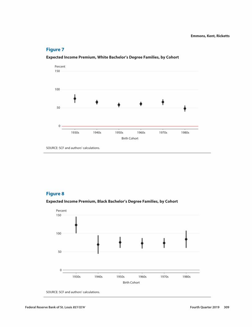
Trends in the Expected Income Premiums for Bachelor’s Degree and Postgraduate Families. We found that the college income premium over otherwise similar nongraduate families—from the same birth decade and race or ethnicity—declined somewhat among White families, on balance, between the 1930s and the 1980s birth cohorts but remained positive (Figure 7). Among Black families, there was no significant change between the 1940s and the 1980s, with all income premiums significantly above zero (Figure 8). The figures show point estimates and corresponding 95 percent confidence intervals.19
The income premium for postgraduate families over nongraduate families was typically higher at the mean relative to that for bachelor’s degree families over nongraduate families (Figures 9 and 10 for Whites and Blacks, respectively, and Figures A3 and A4 for Hispanics and other non-White families, respectively). The income premium for postgraduate White families followed a more pronounced downward trajectory than that for White bachelor’s degree families but remained positive for all cohorts. Among Black postgraduate families, the income premium ranged more widely and was large for all cohorts.20 In sum, the post-graduate families of all races and ethnicities from all six birth decades that we consider enjoy a clear income advantage over families without at least a bachelor’s degree.
Household Net Worth. Household net worth, also adjusted for household size, is our preferred measure of wealth. The SCF is considered the gold standard of balance sheet infor-mation precisely because of its detailed accounting of household assets and liabilities. Family net worth is the difference between a family’s assets and its debts at a point in time. Total assets include both financial assets, such as bank accounts, mutual funds, and securities, and tangible assets, including real estate, vehicles, and durable goods. Total debt includes home-secured borrowing (mortgages), other secured borrowing (such as vehicle loans), and unsecured debts (such as credit cards and student loans). Debt incurred in association with a privately owned business or to finance investment in real estate is subtracted from the asset’s value, rather than being included in the family’s debt. All wealth figures also are adjusted for inflation.
We adjust net worth for household size as for income:
(3) Wi = wi
Hi.
Our wealth specification has the same structural form (explanatory variables and their inter-actions) as that used to estimate the income premium. However, the transformation used for the dependent variable (W) is the inverse hyperbolic sine (IHS) transformation rather than the natural log.21 The transformed dependent variable is given by
(4) sinh−1 θWi( )= ln θWi + θ 2Wi2 +1( )
12
⎡
⎣⎢
⎤
⎦⎥ /θ ,
Emmons, Kent, Ricketts
Federal Reserve Bank of St. Louis REVIEW Fourth Quarter 2019 309
0
50
100
150
1930s 1940s 1950s 1960s 1970s 1980s
Percent
Birth Cohort
Figure 8Expected Income Premium, Black Bachelor’s Degree Families, by Cohort
SOURCE: SCF and authors’ calculations.
0
50
100
150
1930s 1940s 1950s 1960s 1970s 1980s
Percent
Birth Cohort
Figure 7Expected Income Premium, White Bachelor’s Degree Families, by Cohort
SOURCE: SCF and authors’ calculations.

Emmons, Kent, Ricketts
310 Fourth Quarter 2019 Federal Reserve Bank of St. Louis REVIEW
0
50
100
150
1930s 1940s 1950s 1960s 1970s 1980s
Percent
Birth Cohort
Figure 10Expected Income Premium, Black Postgraduate Families, by Cohort
SOURCE: SCF and authors’ calculations.
0
50
100
150
1930s 1940s 1950s 1960s 1970s 1980s
Percent
Birth Cohort
Figure 9Expected Income Premium, White Postgraduate Families, by Cohort
SOURCE: SCF and authors’ calculations.

Emmons, Kent, Ricketts
Federal Reserve Bank of St. Louis REVIEW Fourth Quarter 2019 311
0
200
400
600
1930s 1940s 1950s 1960s 1970s 1980s
Percent
Birth Cohort
Figure 12Expected Wealth Premium, Black Bachelor’s Degree Families, by Cohort
SOURCE: SCF and authors’ calculations.
0
200
400
600
1930s 1940s 1950s 1960s 1970s 1980s
Percent
Birth Cohort
Figure 11Expected Wealth Premium, White Bachelor’s Degree Families, by Cohort
SOURCE: SCF and authors’ calculations.

Emmons, Kent, Ricketts
312 Fourth Quarter 2019 Federal Reserve Bank of St. Louis REVIEW
0
200
400
600
1930s 1940s 1950s 1960s 1970s 1980s
Percent
Birth Cohort
Figure 14Expected Wealth Premium, Black Postgraduate Families, by Cohort
SOURCE: SCF and authors’ calculations.
0
200
400
600
1930s 1940s 1950s 1960s 1970s 1980s
Percent
Birth Cohort
Figure 13Expected Wealth Premium, White Postgraduate Families, by Cohort
SOURCE: SCF and authors’ calculations.

Tabl
e 4
Wea
lth
Regr
essi
ons:
Whi
te F
amili
esD
epen
dent
var
iabl
e: N
et w
orth
Raci
al/e
thni
c gr
oup:
Whi
tePs
eudo
R2 :
0.30
N: 3
7,04
4
(1)
(2)
(3)
(4)
(5)
(6)
Inde
pend
ent v
aria
bles
βSE
H–P(
β)t–
Stat
p–Va
lue
βSE
H–P(
β)t–
Stat
p–Va
lue
βSE
H–P(
β)t–
Stat
p–Va
lue
βSE
H–P(
β)t–
Stat
p–Va
lue
βSE
H–P(
β)t–
Stat
p–Va
lue
βSE
H–P(
β)t–
Stat
p–Va
lue
Inte
rcep
t–2
1,044
2,075
–10.1
40.0
0–2
0,491
2,134
–9.60
0.00
–20,7
582,1
83–9
.510.0
0–2
1,252
2,123
–10.0
10.0
0–2
1,962
2,084
–10.5
40.0
0–2
2,629
1,932
–11.7
10.0
0
Life c
ycle
Age
1,412
127
11.08
0.00
1,412
127
11.08
0.00
1,412
127
11.08
0.00
1,412
127
11.08
0.00
1,412
127
11.08
0.00
1,412
127
11.08
0.00
Age2
–92
–3.90
0.00
–92
–3.90
0.00
–92
–3.90
0.00
–92
–3.90
0.00
–92
–3.90
0.00
–92
–3.90
0.00
Age3
00
0.23
0.82
00
0.23
0.82
00
0.23
0.82
00
0.23
0.82
00
0.23
0.82
00
0.23
0.82
Wea
lth p
rem
ium
Term
inal
four
–yea
r gr
adua
te (G
)12
,451
633
2.47
19.66
0.00
10,82
344
61.9
524
.270.0
010
,476
444
1.85
23.59
0.00
9,791
435
1.66
22.53
0.00
8,483
633
1.34
13.39
0.00
3,511
752
0.42
4.67
0.00
Postg
radu
ate (
P)16
,151
596
4.03
27.10
0.00
15,93
544
93.9
235
.460.0
014
,727
530
3.36
27.77
0.00
13,25
166
12.7
620
.040.0
07,7
0799
51.1
67.7
40.0
02,5
061,2
830.2
81.9
50.0
5
Birth
coho
rts
Born
bef
ore 1
930
or af
ter 1
989
–1,35
438
0–0
.13–3
.560.0
0–1
,907
418
–0.17
–4.56
0.00
–1,64
045
8–0
.15–3
.580.0
0–1
,146
478
–0.11
–2.40
0.02
–436
511
–0.04
–0.85
0.39
232
520
0.02
0.45
0.66
Born
in 19
30s
(Om
itted
)–5
5336
8–0
.05–1
.500.1
3–2
8541
0–0
.03–0
.700.4
920
845
90.0
20.4
50.6
591
848
40.1
01.9
00.0
61,5
8655
40.1
72.8
60.0
0
Born
in 19
40s
553
368
0.06
1.50
0.13
(Om
itted
)26
832
30.0
30.8
30.4
176
137
60.0
82.0
30.0
41,4
7143
90.1
63.3
50.0
02,1
3952
40.2
44.0
80.0
0
Born
in 19
50s
285
410
0.03
0.70
0.49
–268
323
–0.03
–0.83
0.41
(Om
itted
)49
430
90.0
51.6
00.1
11,2
0438
20.1
33.1
50.0
01,8
7149
60.2
13.7
70.0
0
Born
in 19
60s
–208
459
–0.02
–0.45
0.65
–761
376
–0.07
–2.03
0.04
–494
309
–0.05
–1.60
0.11
(Om
itted
)71
033
90.0
72.0
90.0
41,3
7841
10.1
53.3
50.0
0
Born
in 19
70s
–918
484
–0.09
–1.90
0.06
–1,47
143
9–0
.14–3
.350.0
0–1
,204
382
–0.11
–3.15
0.00
–710
339
–0.07
–2.09
0.04
(Om
itted
)66
843
00.0
71.5
50.1
2
Born
in 19
80s
–1,58
655
4–0
.15–2
.860.0
0–2
,139
524
–0.19
–4.08
0.00
–1,87
149
6–0
.17–3
.770.0
0–1
,378
411
–0.13
–3.35
0.00
–668
430
–0.06
–1.55
0.12
(Om
itted
)
Coho
rt X
weal
th p
rem
ium
Born
bef
ore 1
930
or af
ter 1
989 *
G–2
,460
821
–0.22
–2.99
0.00
–831
684
–0.08
–1.22
0.22
–485
725
–0.05
–0.67
0.50
200
677
0.02
0.30
0.77
1,508
849
0.16
1.78
0.08
6,480
960
0.91
6.75
0.00
Born
in 19
30s *
G(O
mitt
ed)
1,629
755
0.18
2.16
0.03
1,975
718
0.22
2.75
0.01
2,660
761
0.30
3.50
0.00
3,968
883
0.49
4.49
0.00
8,940
1,030
1.44
8.68
0.00
Born
in 19
40s *
G–1
,629
755
–0.15
–2.16
0.03
(Om
itted
)34
662
70.0
40.5
50.5
81,0
3165
90.1
11.5
70.1
22,3
3976
60.2
63.0
60.0
07,3
1185
21.0
88.5
90.0
0
Born
in 19
50s *
G–1
,975
718
–0.18
–2.75
0.01
–346
627
–0.03
–0.55
0.58
(Om
itted
)68
560
70.0
71.1
30.2
61,9
9373
90.2
22.7
00.0
16,9
6589
71.0
17.7
70.0
0
Born
in 19
60s *
G–2
,660
761
–0.23
–3.50
0.00
–1,03
165
9–0
.10–1
.570.1
2–6
8560
7–0
.07–1
.130.2
6(O
mitt
ed)
1,308
736
0.14
1.78
0.08
6,280
795
0.87
7.90
0.00
Born
in 19
70s *
G–3
,968
883
–0.33
–4.49
0.00
–2,33
976
6–0
.21–3
.060.0
0–1
,993
739
–0.18
–2.70
0.01
–1,30
873
6–0
.12–1
.780.0
8(O
mitt
ed)
4,972
964
0.64
5.16
0.00
Born
in 19
80s *
* G–8
,940
1,030
–0.59
–8.68
0.00
–7,31
185
2–0
.52–8
.590.0
0–6
,965
897
–0.50
–7.77
0.00
–6,28
079
5–0
.47–7
.900.0
0–4
,972
964
–0.39
–5.16
0.00
(Om
itted
)
Born
bef
ore 1
930
or af
ter 1
989 *
P–1
,369
823
–0.13
–1.66
0.10
–1,15
373
8–0
.11–1
.560.1
255
803
0.01
0.07
0.95
1,531
841
0.17
1.82
0.07
7,075
1,154
1.03
6.13
0.00
12,27
61,2
802.4
19.5
90.0
0
Born
in 19
30s *
P(O
mitt
ed)
216
696
0.02
0.31
0.76
1,424
797
0.15
1.79
0.07
2,900
902
0.34
3.22
0.00
8,444
1,226
1.33
6.89
0.00
13,64
51,3
982.9
19.7
60.0
0
Born
in 19
40s *
P–2
1669
6–0
.02–0
.310.7
6(O
mitt
ed)
1,208
722
0.13
1.67
0.09
2,684
769
0.31
3.49
0.00
8,228
1,125
1.28
7.32
0.00
13,42
91,3
692.8
39.8
10.0
0
Born
in 19
50s *
P–1
,424
797
–0.13
–1.79
0.07
–1,20
872
2–0
.11–1
.670.0
9(O
mitt
ed)
1,476
789
0.16
1.87
0.06
7,020
1,142
1.02
6.14
0.00
12,22
11,4
412.3
98.4
80.0
0
Born
in 19
60s *
P–2
,900
902
–0.25
–3.22
0.00
–2,68
476
9–0
.24–3
.490.0
0–1
,476
789
–0.14
–1.87
0.06
(Om
itted
)5,5
441,1
960.7
44.6
30.0
010
,745
1,329
1.93
8.09
0.00
Born
in 19
70s *
P–8
,444
1,226
–0.57
–6.89
0.00
–8,22
81,1
25–0
.56–7
.320.0
0–7
,020
1,142
–0.50
–6.14
0.00
–5,54
41,1
96–0
.43–4
.630.0
0(O
mitt
ed)
5,201
1,439
0.68
3.61
0.00
Born
in 19
80s *
P–1
3,645
1,398
–0.74
–9.76
0.00
–13,4
291,3
69–0
.74–9
.810.0
0–1
2,221
1,441
–0.71
–8.48
0.00
–10,7
451,3
29–0
.66–8
.090.0
0–5
,201
1,439
–0.41
–3.61
0.00
(Om
itted
)
NO
TE: S
E, s
tand
ard
erro
r. St
anda
rd e
rror
s ar
e bo
otst
rapp
ed w
ith 9
99 re
plic
ates
in a
ccor
danc
e w
ith th
e sa
mpl
e de
sign
and
are
adj
uste
d fo
r im
puta
tion
unce
rtai
nty.
Non
resp
onse
-adj
uste
d sa
mpl
ing
wei
ghts
wer
e al
so u
sed.
Hou
seho
ld-s
ize
adju
sted
net
wor
th w
as tr
ans-
form
ed w
ith th
e in
vers
e hy
perb
olic
sin
e fu
nctio
n, w
ith a
sca
ling
fact
or o
f 0.0
001.
The
Hal
vors
en-P
alm
quis
t tra
nsfo
rmat
ion
prov
ides
a s
imila
r int
erpr
etat
ion
of th
e co
effici
ents
on
bina
ry v
aria
bles
as
that
of a
log-
linea
r mod
el.
SOU
RCE:
SCF
and
aut
hors
’ cal
cula
tions
.

Tabl
e 5
Wea
lth
Regr
essi
ons:
Bla
ck F
amili
esD
epen
dent
var
iabl
e: N
et w
orth
Raci
al/e
thni
c gr
oup:
Bla
ckPs
eudo
R2 :
0.19
N: 5
,186
(1)
(2)
(3)
(4)
(5)
(6)
Inde
pend
ent v
aria
bles
βSE
H–P(
β)t–
Stat
p–Va
lue
βSE
H–P(
β)t–
Stat
p–Va
lue
βSE
H–P(
β)t–
Stat
p–Va
lue
βSE
H–P(
β)t–
Stat
p–Va
lue
βSE
H–P(
β)t–
Stat
p–Va
lue
βSE
H–P(
β)t–
Stat
p–Va
lue
Inte
rcep
t1,8
193,0
490.6
00.5
53,1
343,1
790.9
90.3
21,4
953,3
990.4
40.6
61,2
943,3
350.3
90.7
01,7
933,2
100.5
60.5
8–9
283,2
25–0
.290.7
7
Life c
ycle
Age
–74
222
–0.33
0.74
–74
222
–0.33
0.74
–74
222
–0.33
0.74
–74
222
–0.33
0.74
–74
222
–0.33
0.74
–74
222
–0.33
0.74
Age2
105
2.22
0.03
105
2.22
0.03
105
2.22
0.03
105
2.22
0.03
105
2.22
0.03
105
2.22
0.03
Age3
00
–2.69
0.01
00
–2.69
0.01
00
–2.69
0.01
00
–2.69
0.01
00
–2.69
0.01
00
–2.69
0.01
Wea
lth p
rem
ium
Term
inal
four
–yea
r gr
adua
te (G
)18
,075
1,680
5.09
10.76
0.00
12,62
61,5
032.5
38.4
00.0
08,1
511,4
431.2
65.6
50.0
010
,201
1,115
1.77
9.15
0.00
1,662
1,420
0.18
1.17
0.24
540
1,799
0.06
0.30
0.76
Postg
radu
ate (
P)16
,542
3,115
4.23
5.31
0.00
18,07
31,4
105.0
912
.820.0
014
,631
1,817
3.32
8.05
0.00
1,664
2,487
0.18
0.67
0.50
1,468
2,844
0.16
0.52
0.61
761
3,706
0.08
0.21
0.84
Birth
coho
rts
Born
bef
ore 1
930
or af
ter 1
989
–2,31
290
0–0
.21–2
.570.0
1–3
,626
815
–0.30
–4.45
0.00
–1,98
785
9–0
.18–2
.310.0
2–1
,786
865
–0.16
–2.07
0.04
–2,28
687
8–0
.20–2
.600.0
143
583
80.0
40.5
20.6
0
Born
in 19
30s
(Om
itted
)–1
,314
757
–0.12
–1.74
0.08
325
867
0.03
0.37
0.71
525
844
0.05
0.62
0.53
2686
40.0
00.0
30.9
82,7
4791
50.3
23.0
00.0
0
Born
in 19
40s
1,314
757
0.14
1.74
0.08
(Om
itted
)1,6
3963
20.1
82.5
90.0
11,8
4065
30.2
02.8
20.0
01,3
4075
50.1
41.7
70.0
84,0
6170
80.5
05.7
40.0
0
Born
in 19
50s
–325
867
–0.03
–0.37
0.71
–1,63
963
2–0
.15–2
.590.0
1(O
mitt
ed)
201
568
0.02
0.35
0.72
–299
715
–0.03
–0.42
0.68
2,422
673
0.27
3.60
0.00
Born
in 19
60s
–525
844
–0.05
–0.62
0.53
–1,84
065
3–0
.17–2
.820.0
0–2
0156
8–0
.02–0
.350.7
2(O
mitt
ed)
–500
612
–0.05
–0.82
0.41
2,222
590
0.25
3.77
0.00
Born
in 19
70s
–26
864
0.00
–0.03
0.98
–1,34
075
5–0
.13–1
.770.0
829
971
50.0
30.4
20.6
850
061
20.0
50.8
20.4
1(O
mitt
ed)
2,721
624
0.31
4.36
0.00
Born
in 19
80s
–2,74
791
5–0
.24–3
.000.0
0–4
,061
708
–0.33
–5.74
0.00
–2,42
267
3–0
.22–3
.600.0
0–2
,222
590
–0.20
–3.77
0.00
–2,72
162
4–0
.24–4
.360.0
0(O
mitt
ed)
Coho
rt X
weal
th p
rem
ium
Born
bef
ore 1
930
or af
ter 1
989 *
G–1
6,824
4,133
–0.81
–4.07
0.00
–11,3
754,0
62–0
.68–2
.800.0
1–6
,901
3,924
–0.50
–1.76
0.08
–8,95
03,9
61–0
.59–2
.260.0
2–4
123,9
34–0
.04–0
.100.9
271
04,1
910.0
70.1
70.8
7
Born
in 19
30s *
G(O
mitt
ed)
5,449
2,260
0.72
2.41
0.02
9,923
2,246
1.70
4.42
0.00
7,874
2,041
1.20
3.86
0.00
16,41
22,1
804.1
67.5
30.0
017
,535
2,575
4.77
6.81
0.00
Born
in 19
40s *
G–5
,449
2,260
–0.42
–2.41
0.02
(Om
itted
)4,4
742,2
890.5
61.9
50.0
52,4
251,8
580.2
71.3
10.1
910
,964
2,204
1.99
4.98
0.00
12,08
62,4
312.3
54.9
70.0
0
Born
in 19
50s *
G–9
,923
2,246
–0.63
–4.42
0.00
–4,47
42,2
89–0
.36–1
.950.0
5(O
mitt
ed)
–2,04
91,7
63–0
.19–1
.160.2
56,4
892,0
450.9
13.1
70.0
07,6
112,0
961.1
43.6
30.0
0
Born
in 19
60s *
G–7
,874
2,041
–0.54
–3.86
0.00
–2,42
51,8
58–0
.22–1
.310.1
92,0
491,7
630.2
31.1
60.2
5(O
mitt
ed)
8,539
1,738
1.35
4.91
0.00
9,661
2,053
1.63
4.71
0.00
Born
in 19
70s *
G–1
6,412
2,180
–0.81
–7.53
0.00
–10,9
642,2
04–0
.67–4
.980.0
0–6
,489
2,045
–0.48
–3.17
0.00
–8,53
91,7
38–0
.57–4
.910.0
0(O
mitt
ed)
1,122
2,405
0.12
0.47
0.64
Born
in 19
80s *
* G–1
7,535
2,575
–0.83
–6.81
0.00
–12,0
862,4
31–0
.70–4
.970.0
0–7
,611
2,096
–0.53
–3.63
0.00
–9,66
12,0
53–0
.62–4
.710.0
0–1
,122
2,405
–0.11
–0.47
0.64
(Om
itted
)
Born
bef
ore 1
930
or af
ter 1
989 *
P–9
,777
6,462
–0.62
–1.51
0.13
–11,3
076,2
20–0
.68–1
.820.0
7–7
,865
6,398
–0.54
–1.23
0.22
5,102
6,451
0.67
0.79
0.43
5,298
6,163
0.70
0.86
0.39
6,004
6,725
0.82
0.89
0.37
Born
in 19
30s *
P(O
mitt
ed)
–1,53
13,2
50–0
.14–0
.470.6
41,9
123,7
300.2
10.5
10.6
114
,879
4,227
3.43
3.52
0.00
15,07
54,2
013.5
23.5
90.0
015
,781
5,345
3.85
2.95
0.00
Born
in 19
40s *
P1,5
313,2
500.1
70.4
70.6
4(O
mitt
ed)
3,442
2,315
0.41
1.49
0.14
16,40
92,9
144.1
65.6
30.0
016
,605
3,172
4.26
5.24
0.00
17,31
14,2
584.6
54.0
70.0
0
Born
in 19
50s *
P–1
,912
3,730
–0.17
–0.51
0.61
–3,44
22,3
15–0
.29–1
.490.1
4(O
mitt
ed)
12,96
72,9
872.6
64.3
40.0
013
,163
3,619
2.73
3.64
0.00
13,86
94,1
533.0
03.3
40.0
0
Born
in 19
60s *
P–1
4,879
4,227
–0.77
–3.52
0.00
–16,4
092,9
14–0
.81–5
.630.0
0–1
2,967
2,987
–0.73
–4.34
0.00
(Om
itted
)19
63,9
210.0
20.0
50.9
690
24,2
850.0
90.2
10.8
3
Born
in 19
70s *
P–1
5,075
4,201
–0.78
–3.59
0.00
–16,6
053,1
72–0
.81–5
.240.0
0–1
3,163
3,619
–0.73
–3.64
0.00
–196
3,921
–0.02
–0.05
0.96
(Om
itted
)70
65,3
490.0
70.1
30.8
9
Born
in 19
80s *
P–1
5,781
5,345
–0.79
–2.95
0.00
–17,3
114,2
58–0
.82–4
.070.0
0–1
3,869
4,153
–0.75
–3.34
0.00
–902
4,285
–0.09
–0.21
0.83
–706
5,349
–0.07
–0.13
0.89
(Om
itted
)
NO
TE: S
E, s
tand
ard
erro
r. Se
e Ta
ble
4 no
te.
SOU
RCE:
SCF
and
aut
hors
’ cal
cula
tions
.

Emmons, Kent, Ricketts
Federal Reserve Bank of St. Louis REVIEW Fourth Quarter 2019 315
where θ is a scaling parameter, which controls how much of the function’s domain is approxi-mately linear and how much resembles the natural logarithm. The IHS transformation is quite useful when working with wealth outcomes because it can accommodate negative and zero balances (unlike the natural log transformation). The scaling parameter is estimated using maximum likelihood, and we use 0.0001 as is typical in the literature.22
As shown in Halvorsen and Palmquist (1980), unlike in a log-linear model, the expected change in wealth attributed to a terminal four-year degree and postgraduate degree is not simply 100 × β4 and 100 × β5. The semi-logarithmic nature of the IHS requires a modified form of the Halvorsen-Palmquist transformation to provide a similar percentage-change interpretation. We use the same form as that used in Gale and Pence (2006): eβθ – 1.
Similar to the regressions of income, we estimate six variations of our wealth specification, switching the omitted birth cohort for each decade. Again, due to considerably different wealth life cycles and historical context, we estimate regressions separately for the four racial and ethnic groups available within the SCF (Tables 4 and 5 for White and Black families, respec-tively, and Tables A4 and A5 for Hispanic and other families, respectively).
Trends in the Estimated Wealth Premiums of College Graduates. In contrast to rela-tively stable income premiums across successive birth decades, the wealth premium enjoyed by bachelor’s degree families over otherwise demographically similar nongraduate families declined progressively between the 1930s and 1980s cohorts. Among White bachelor’s degree families, for example, the 1930s cohort owned 247 percent more wealth and the 1940s cohort owned 195 percent more wealth than nongraduate families of the same age, but the 1980s cohort owned only 42 percent more wealth (Figure 11).
Among Black bachelor’s degree families, the wealth premium peaked at 509 percent in the 1930s cohort, fell to 177 percent for the 1960s cohort, and was statistically indistinguish-able from zero for both the 1970s and the 1980s cohorts (Figure 12). In other words, we cannot reject the null hypothesis that the average Black bachelor’s degree family with a head born between 1970 and 1989 had no more wealth than the average Black nongraduate family with a head born in the same decade.
To be clear, these estimates take into account the fact that the older cohorts have had more time to accumulate wealth than the younger cohorts. Our models explicitly adjust for age by including a flexible life cycle component in each specification. Our estimates of wealth pre-miums are conditional on the amount of wealth accumulation we would expect at any given age.
The results are even starker among postgraduate families. Among White postgraduate families, the 403 percent wealth premium enjoyed by members of the 1930s cohort had shrunk to only 116 percent and 28 percent for the 1970s and 1980s cohorts, respectively (Figure 13). The drop-off for this 1970s cohort is much steeper than that for White bachelor’s degree families in the same cohort. For the 1980s cohort, the expected wealth premium for White postgraduate families over nongraduate families is statistically indistinguishable from zero at standard confidence levels. The t-statistic estimated for β5 falls to 1.95, just below the threshold for rejecting the null hypothesis that β5 = 0.23
Among Black postgraduate families, the expected wealth premium ranged from 509 per-cent for the 1940s cohort to levels slightly above but statistically indistinguishable from zero

Emmons, Kent, Ricketts
316 Fourth Quarter 2019 Federal Reserve Bank of St. Louis REVIEW
for cohorts born in the 1960s, 1970s, and 1980s (Figure 14). This suggests that, on average, postgraduate Black families with heads born in the 1960s, 1970s, or 1980s have not accumu-lated more wealth than Black nongraduate families with heads born in the same decades.
In sum, Whites are the only racial or ethnic group born in the 1980s for whom a bachelor’s degree provides a family with a reliable wealth advantage over comparable nongraduate fam-ilies—albeit one that is much smaller than those enjoyed by earlier cohorts of college gradu-ates. Even more surprisingly, the expected wealth premium among postgraduate families with a head born in the 1980s is indistinguishable from zero at standard confidence levels for all races and ethnicities.24
3 WHY HAS THE COLLEGE INCOME PREMIUM BEEN MORE DURABLE THAN THE WEALTH PREMIUM?
Why has the college wealth premium for college graduates over nongraduates declined in successive cohorts? And why do generational trends in wealth accumulation differ so mark-edly from those for income? Plausible explanations for a declining college wealth premium across successive birth cohorts—even while the college income premium remains largely intact—must satisfy three criteria:
• The explanation describes factors that affect wealth accumulation differently from how they affect income.
• The explanation is consistent with a decline in the college wealth premium that has been underway for many decades, with a large cumulative effect.
• The explanation is not primarily related to the racial and ethnic mix, the educational attainment, or the average family size of particular cohorts, since our premium esti-mates explicitly control for these elements.
We offer three categories of explanations that appear plausible in the sense that they sat-isfy the criteria outlined above. We leave for future research a detailed investigation of these hypotheses.
First Plausible Explanation: Aggregate Wealth Fluctuations. A favorable or unfavor-able financial climate may play a role in explaining large differences in wealth accumulation across cohorts. A generation that acquires assets when asset prices or valuations are low has an advantage over a subsequent generation that accumulates assets when they are expensive. Gale and Pence (2006) found that differences in the amount of capital gains received by vari-ous birth cohorts were substantial in SCF data through 2001.
The working-paper version of this article includes a simulation of wealth accumulation by cohorts born at different times in the presence of large fluctuations in asset valuations over time.25 That exercise demonstrated that the three oldest cohorts we studied generally have experienced fortuitous asset price fluctuations. This explanation has little to say about the very low wealth premiums we estimate for the 1980s cohort, however, which had little asset accumulation by the end of our sample period.

Emmons, Kent, Ricketts
Federal Reserve Bank of St. Louis REVIEW Fourth Quarter 2019 317
Second Plausible Explanation: Financial Liberalization. Accumulation of financial knowledge takes time, so young college graduates are potentially vulnerable to making finan-cial mistakes.26 A highly deregulated financial environment is one in which those who are less financially savvy, including young people, have greater access to credit and consequently greater risk associated with managing more consumer debt.
The explosion of consumer debt beginning in the early 1980s has been remarkable. The long-term increase in debt and debt burden has been particularly large for younger cohorts.27 Additionally, debt ratios generally are higher among college graduates than nongraduates. The leveraging of college-graduate balance sheets over time is entirely consistent with the progressive weakening of their overall financial positions that we identified—even while the college and postgraduate income premiums remained intact.
Third Plausible Explanation: Rising Cost of College. A secular increase in the cost of attending college checks all of the boxes as a plausible explanation for our findings—it directly affects wealth, not income; it is a long-running story; and it is unrelated to changes in the demographics of college graduates for which we could control.
While the overall level of consumer prices has increased by a factor of four since 1978, the cost of college tuition and fees has increased by a factor of almost 14—more than triple the overall increase in consumer prices.28 Moreover, the rate of excess tuition increases—the amount by which college-tuition inflation exceeded overall inflation—increased after 2000. If the secular increase in the cost of attending college is part of the explanation of progressively weaker wealth outcomes across cohorts, then an acceleration of college costs might show up as a marked deterioration in wealth for the affected cohorts. This is, in fact, what we find—the 1980s cohort of college graduates, most of whom attended college after 2000, experienced a very sharp decline in wealth outcomes.
4 SUMMARY AND CONCLUSIONSUsing the Federal Reserve’s Survey of Consumer Finances, we showed that large and
increasing income and wealth premiums in aggregate data associated with families whose heads have a bachelor’s or higher over families whose heads have no postsecondary degree are misleading. Comparing bachelor’s degree and postgraduate families to nongraduate fam-ilies of the same race and ethnicity born in the same decade, we confirmed that the income premium generally remains positive for all birth decades between the 1930s and the 1980s. However, the premium may have declined somewhat among the most recent cohort (1980s) of White families.
We found a different pattern for the wealth premium. A high and rising wealth premium enjoyed by the average bachelor’s degree family and the average postgraduate family in aggre-gate data in fact masks a lower and declining premium across successive birth cohorts. Among families with heads born in the 1980s, the college wealth premium weakens to the point of statistical insignificance with the single exception of White bachelor’s degree families, for which it remains positive but much smaller than that enjoyed by previous cohorts. Results were similar for all races and ethnicities.

Emmons, Kent, Ricketts
318 Fourth Quarter 2019 Federal Reserve Bank of St. Louis REVIEW
Thus, the promise of economic and financial advantages associated with postsecondary degrees remains only partially supported by the most recent data. Careful analysis by birth decade and race and ethnicity is required to identify diverging trends for income and wealth premiums over time. n
APPENDIX A
Table A1Variable Descriptions
Variable Description Source
Household size- adjusted net worth
Inflation-adjusted net worth divided by the square root of household size. Networth (Board)
Household size- adjusted income
Inflation-adjusted income divided by the square root of household size. Income (Board)
Household sizeNumber of people in the household according to the HHL. Excludes people included in the household listing who do not usually live there and who are financially independent.
X101
Age Respondent's age. X14
Age2 Respondent's age squared. X14
Age3 Respondent's age cubed. X14
4-Year college graduateMaximum educational attainment of household respondent was a 4-year college degree (e.g., BA, AB, BS).
1989-2013: X5901, X5904, X5905; 2016: X5931
Postgraduate
Maximum educational attainment of household respondent was a post-graduate degree. This includes master's degrees (e.g. MA, MS, MENG, MED, MSW, MBA), professional degrees (e.g., MD, DDS, DVM, LLB, JD), and doctoral degrees (e.g., PhD, EDD).
1989-2013: X5901, X5904, X5905; 2016: X5931
White Respondent identified the race or ethnicity that best describes them as White. X6809
BlackRespondent identified the race or ethnicity that best describes them as Black/African-American.
X6809
HispanicRespondent identified the race or ethnicity that best describes them as Hispanic/Latino.
X6809
Other
Respondent identified the race or ethnicity that best describes them as Asian or American Indian/Alaska Native or Native Hawaiian/Pacific Islander or Other or identified with multiple races or ethnicities. NOTE: All of these responses are combined by Board staff for confidentiality reasons.
X6809
Birth cohorts
Six birth cohorts represented by binary variables equal to one if the survey respondent was born within the respective decade. Decades include: 1930s, 1940s, 1950s, 1960s, 1970s, and 1980s. Respondents born prior to 1930 or after 1989 were represented by a "catch-all" binary variable and included in regressions to avoid perfect multicolinearity. Results for this variable were not included in analysis.
Survey year, X14
NOTE: These variables are available in all survey waves from 1989-2016.
SOURCE: SCF and authors’ calculations.

Tabl
e A
2In
com
e Re
gres
sion
s: H
ispa
nic
Fam
ilies
Dep
ende
nt v
aria
ble:
Inco
me
Raci
al/e
thni
c gr
oup:
His
pani
c, a
ny R
ace
Pseu
do R
2 : 0.
10N
: 3,5
53
(1)
(2)
(3)
(4)
(5)
(6)
Inde
pend
ent v
aria
bles
βSE
t–St
atp–
Valu
eβ
SEt–
Stat
p–Va
lue
βSE
t–St
atp–
Valu
eβ
SEt–
Stat
p–Va
lue
βSE
t–St
atp–
Valu
eβ
SEt–
Stat
p–Va
lue
Inte
rcep
t7.
070.
3023
.61
0.00
6.93
0.30
23.2
30.
006.
970.
3122
.55
0.00
6.92
0.30
22.7
20.
007.
050.
3122
.75
0.00
7.28
0.29
24.7
50.
00
Life
cyc
le
Age
0.14
0.02
7.01
0.00
0.14
0.02
7.01
0.00
0.14
0.02
7.01
0.00
0.14
0.02
7.01
0.00
0.14
0.02
7.01
0.00
0.14
0.02
7.01
0.00
Age
20.
000.
00–4
.95
0.00
0.00
0.00
–4.9
50.
000.
000.
00–4
.95
0.00
0.00
0.00
–4.9
50.
000.
000.
00–4
.95
0.00
0.00
0.00
–4.9
50.
00
Age
30.
000.
003.
280.
000.
000.
003.
280.
000.
000.
003.
280.
000.
000.
003.
280.
000.
000.
003.
280.
000.
000.
003.
280.
00
Inco
me
prem
ium
Term
inal
four
–yea
r gr
adua
te (G
)0.
400.
211.
890.
060.
340.
400.
870.
390.
770.
126.
300.
000.
440.
123.
830.
000.
870.
0711
.90
0.00
0.56
0.10
5.69
0.00
Post
grad
uate
(P)
1.11
0.14
8.07
0.00
1.39
0.15
9.27
0.00
1.11
0.15
7.35
0.00
1.04
0.15
6.83
0.00
0.93
0.12
8.01
0.00
1.00
0.10
10.3
40.
00
Birt
h co
hort
s
Born
bef
ore
1930
or
aft
er 1
989
–0.2
70.
12–2
.22
0.03
–0.1
30.
11–1
.18
0.24
–0.1
60.
12–1
.42
0.15
–0.1
20.
11–1
.10
0.27
–0.2
50.
12–2
.07
0.04
–0.4
80.
11–4
.24
0.00
Born
in 1
930s
(Om
itted
)0.
140.
091.
560.
120.
100.
091.
120.
260.
150.
111.
440.
150.
020.
100.
190.
85–0
.21
0.11
–1.9
10.
06
Born
in 1
940s
–0.1
40.
09–1
.56
0.12
(Om
itted
)–0
.04
0.06
–0.6
40.
520.
010.
070.
110.
91–0
.12
0.07
–1.6
50.
10–0
.35
0.08
–4.2
40.
00
Born
in 1
950s
–0.1
00.
09–1
.12
0.26
0.04
0.06
0.64
0.52
(Om
itted
)0.
050.
060.
780.
44–0
.08
0.05
–1.6
20.
11–0
.31
0.07
–4.7
60.
00
Born
in 1
960s
–0.1
50.
11–1
.44
0.15
–0.0
10.
07–0
.11
0.91
–0.0
50.
06–0
.78
0.44
(Om
itted
)–0
.13
0.06
–2.2
20.
03–0
.36
0.06
–5.6
10.
00
Born
in 1
970s
–0.0
20.
10–0
.19
0.85
0.12
0.07
1.65
0.10
0.08
0.05
1.62
0.11
0.13
0.06
2.22
0.03
(Om
itted
)–0
.23
0.04
–5.2
30.
00
Born
in 1
980s
0.21
0.11
1.91
0.06
0.35
0.08
4.24
0.00
0.31
0.07
4.76
0.00
0.36
0.06
5.61
0.00
0.23
0.04
5.23
0.00
(Om
itted
)
Coho
rt X
inco
me
prem
ium
Born
bef
ore
1930
or
aft
er 1
989
* G
–0.0
30.
31–0
.09
0.93
0.03
0.47
0.06
0.95
–0.4
00.
26–1
.52
0.13
–0.0
70.
27–0
.27
0.79
–0.5
00.
24–2
.07
0.04
–0.1
90.
25–0
.75
0.46
Born
in 1
930s
* G
(Om
itted
)0.
050.
470.
120.
91–0
.37
0.25
–1.4
80.
14–0
.05
0.25
–0.1
90.
85–0
.47
0.23
–2.1
00.
04–0
.16
0.24
–0.6
90.
49
Born
in 1
940s
* G
–0.0
50.
47–0
.12
0.91
(Om
itted
)–0
.42
0.42
–1.0
10.
31–0
.10
0.41
–0.2
40.
81–0
.53
0.40
–1.3
10.
19–0
.22
0.41
–0.5
30.
59
Born
in 1
950s
* G
0.37
0.25
1.48
0.14
0.42
0.42
1.01
0.31
(Om
itted
)0.
320.
181.
840.
07–0
.11
0.14
–0.7
40.
460.
210.
171.
220.
22
Born
in 1
960s
* G
0.05
0.25
0.19
0.85
0.10
0.41
0.24
0.81
–0.3
20.
18–1
.84
0.07
(Om
itted
)–0
.43
0.13
–3.3
90.
00–0
.12
0.13
–0.8
90.
38
Born
in 1
970s
* G
0.47
0.23
2.10
0.04
0.53
0.40
1.31
0.19
0.11
0.14
0.74
0.46
0.43
0.13
3.39
0.00
(Om
itted
)0.
310.
112.
900.
00
Born
in 1
980s
**
G0.
160.
240.
690.
490.
220.
410.
530.
59–0
.21
0.17
–1.2
20.
220.
120.
130.
890.
38–0
.31
0.11
–2.9
00.
00(O
mitt
ed)
Born
bef
ore
1930
or
aft
er 1
989
* P
0.25
0.45
0.55
0.58
–0.0
30.
47–0
.07
0.94
0.24
0.44
0.56
0.58
0.31
0.42
0.73
0.47
0.43
0.43
0.99
0.32
0.35
0.44
0.79
0.43
Born
in 1
930s
* P
(Om
itted
)–0
.28
0.20
–1.4
20.
160.
000.
21–0
.02
0.99
0.06
0.19
0.31
0.75
0.18
0.18
0.99
0.32
0.10
0.15
0.67
0.50
Born
in 1
940s
* P
0.28
0.20
1.42
0.16
(Om
itted
)0.
280.
221.
290.
200.
340.
221.
550.
120.
460.
202.
260.
020.
390.
172.
300.
02
Born
in 1
950s
* P
0.00
0.21
0.02
0.99
–0.2
80.
22–1
.29
0.20
(Om
itted
)0.
060.
220.
290.
770.
180.
190.
950.
340.
110.
170.
630.
53
Born
in 1
960s
* P
–0.0
60.
19–0
.31
0.75
–0.3
40.
22–1
.55
0.12
–0.0
60.
22–0
.29
0.77
(Om
itted
)0.
120.
190.
620.
530.
040.
210.
200.
84
Born
in 1
970s
* P
–0.1
80.
18–0
.99
0.32
–0.4
60.
20–2
.26
0.02
–0.1
80.
19–0
.95
0.34
–0.1
20.
19–0
.62
0.53
(Om
itted
)–0
.07
0.15
–0.4
90.
63
Born
in 1
980s
* P
–0.1
00.
15–0
.67
0.50
–0.3
90.
17–2
.30
0.02
–0.1
10.
17–0
.63
0.53
–0.0
40.
21–0
.20
0.84
0.07
0.15
0.49
0.63
(Om
itted
)
NO
TE: S
E, s
tand
ard
erro
r. Se
e Ta
ble
2 no
te.
SOU
RCE:
SCF
and
aut
hors
’ cal
cula
tions
.

Tabl
e A
3In
com
e Re
gres
sion
s: F
amili
es o
f Oth
er R
aces
Dep
ende
nt v
aria
ble:
Inco
me
Raci
al/e
thni
c gr
oup:
Oth
er R
aces
Pseu
do R
2 : 0.
20N
: 1,9
93
(1)
(2)
(3)
(4)
(5)
(6)
Inde
pend
ent v
aria
bles
βSE
t–St
atp–
Valu
eβ
SEt–
Stat
p–Va
lue
βSE
t–St
atp–
Valu
eβ
SEt–
Stat
p–Va
lue
βSE
t–St
atp–
Valu
eβ
SEt–
Stat
p–Va
lue
Inte
rcep
t5.
890.
708.
370.
006.
000.
718.
420.
005.
860.
737.
970.
005.
790.
727.
990.
005.
880.
777.
680.
006.
140.
718.
640.
00
Life
cyc
le
Age
0.23
0.05
4.83
0.00
0.23
0.05
4.83
0.00
0.23
0.05
4.83
0.00
0.23
0.05
4.83
0.00
0.23
0.05
4.83
0.00
0.23
0.05
4.83
0.00
Age
20.
000.
00–3
.98
0.00
0.00
0.00
–3.9
80.
000.
000.
00–3
.98
0.00
0.00
0.00
–3.9
80.
000.
000.
00–3
.98
0.00
0.00
0.00
–3.9
80.
00
Age
30.
000.
003.
270.
000.
000.
003.
270.
000.
000.
003.
270.
000.
000.
003.
270.
000.
000.
003.
270.
000.
000.
003.
270.
00
Inco
me
prem
ium
Term
inal
four
–yea
r gr
adua
te (G
)0.
370.
201.
820.
070.
550.
143.
900.
000.
430.
182.
380.
020.
690.
135.
420.
000.
590.
173.
520.
000.
530.
143.
670.
00
Post
grad
uate
(P)
1.25
0.17
7.18
0.00
1.28
0.10
12.5
90.
001.
080.
138.
190.
001.
070.
1010
.36
0.00
1.19
0.12
10.0
70.
000.
720.
135.
560.
00
Birt
h co
hort
s
Born
bef
ore
1930
or
aft
er 1
989
–0.2
80.
23–1
.20
0.23
–0.3
80.
22–1
.71
0.09
–0.2
40.
20–1
.17
0.24
–0.1
70.
20–0
.86
0.39
–0.2
60.
20–1
.34
0.18
–0.5
20.
21–2
.48
0.01
Born
in 1
930s
(Om
itted
)–0
.11
0.14
–0.7
50.
450.
040.
150.
260.
790.
110.
160.
660.
510.
010.
170.
080.
93–0
.24
0.17
–1.4
40.
15
Born
in 1
940s
0.11
0.14
0.75
0.45
(Om
itted
)0.
140.
101.
450.
150.
210.
121.
810.
070.
120.
140.
860.
39–0
.14
0.13
–1.0
60.
29
Born
in 1
950s
–0.0
40.
15–0
.26
0.79
–0.1
40.
10–1
.45
0.15
(Om
itted
)0.
070.
110.
650.
52–0
.03
0.12
–0.2
00.
84–0
.28
0.12
–2.4
00.
02
Born
in 1
960s
–0.1
10.
16–0
.66
0.51
–0.2
10.
12–1
.81
0.07
–0.0
70.
11–0
.65
0.52
(Om
itted
)–0
.09
0.13
–0.7
30.
47–0
.35
0.13
–2.7
40.
01
Born
in 1
970s
–0.0
10.
17–0
.08
0.93
–0.1
20.
14–0
.86
0.39
0.03
0.12
0.20
0.84
0.09
0.13
0.73
0.47
(Om
itted
)–0
.26
0.14
–1.7
90.
07
Born
in 1
980s
0.24
0.17
1.44
0.15
0.14
0.13
1.06
0.29
0.28
0.12
2.40
0.02
0.35
0.13
2.74
0.01
0.26
0.14
1.79
0.07
(Om
itted
)
Coho
rt X
inco
me
prem
ium
Born
bef
ore
1930
or
aft
er 1
989
* G
–0.3
00.
40–0
.76
0.45
–0.4
80.
36–1
.34
0.18
–0.3
60.
37–0
.96
0.34
–0.6
20.
36–1
.75
0.08
–0.5
10.
36–1
.45
0.15
–0.4
50.
37–1
.22
0.22
Born
in 1
930s
* G
(Om
itted
)–0
.18
0.24
–0.7
40.
46–0
.06
0.28
–0.2
00.
84–0
.32
0.26
–1.2
50.
21–0
.21
0.24
–0.8
90.
38–0
.15
0.25
–0.6
30.
53
Born
in 1
940s
* G
0.18
0.24
0.74
0.46
(Om
itted
)0.
120.
230.
510.
61–0
.14
0.19
–0.7
70.
44–0
.04
0.20
–0.1
80.
860.
020.
200.
120.
90
Born
in 1
950s
* G
0.06
0.28
0.20
0.84
–0.1
20.
23–0
.51
0.61
(Om
itted
)–0
.26
0.21
–1.2
50.
21–0
.16
0.26
–0.6
10.
54–0
.10
0.23
–0.4
30.
67
Born
in 1
960s
* G
0.32
0.26
1.25
0.21
0.14
0.19
0.77
0.44
0.26
0.21
1.25
0.21
(Om
itted
)0.
110.
210.
510.
610.
170.
170.
980.
33
Born
in 1
970s
* G
0.21
0.24
0.89
0.38
0.04
0.20
0.18
0.86
0.16
0.26
0.61
0.54
–0.1
10.
21–0
.51
0.61
(Om
itted
)0.
060.
220.
270.
79
Born
in 1
980s
**
G0.
150.
250.
630.
53–0
.02
0.20
–0.1
20.
900.
100.
230.
430.
67–0
.17
0.17
–0.9
80.
33–0
.06
0.22
–0.2
70.
79(O
mitt
ed)
Born
bef
ore
1930
or
aft
er 1
989
* P
0.03
0.39
0.07
0.95
0.00
0.39
0.00
1.00
0.20
0.38
0.52
0.60
0.21
0.39
0.55
0.58
0.09
0.38
0.23
0.82
0.56
0.39
1.43
0.15
Born
in 1
930s
* P
(Om
itted
)–0
.02
0.21
–0.1
20.
900.
170.
200.
860.
390.
190.
181.
010.
310.
060.
210.
290.
770.
530.
202.
640.
01
Born
in 1
940s
* P
0.02
0.21
0.12
0.90
(Om
itted
)0.
200.
161.
260.
210.
210.
151.
430.
150.
090.
150.
560.
570.
560.
173.
380.
00
Born
in 1
950s
* P
–0.1
70.
20–0
.86
0.39
–0.2
00.
16–1
.26
0.21
(Om
itted
)0.
010.
160.
090.
93–0
.11
0.15
–0.7
60.
450.
360.
162.
210.
03
Born
in 1
960s
* P
–0.1
90.
18–1
.01
0.31
–0.2
10.
15–1
.43
0.15
–0.0
10.
16–0
.09
0.93
(Om
itted
)–0
.13
0.15
–0.8
60.
390.
350.
172.
030.
04
Born
in 1
970s
* P
–0.0
60.
21–0
.29
0.77
–0.0
90.
15–0
.56
0.57
0.11
0.15
0.76
0.45
0.13
0.15
0.86
0.39
(Om
itted
)0.
470.
182.
650.
01
Born
in 1
980s
* P
–0.5
30.
20–2
.64
0.01
–0.5
60.
17–3
.38
0.00
–0.3
60.
16–2
.21
0.03
–0.3
50.
17–2
.03
0.04
–0.4
70.
18–2
.65
0.01
(Om
itted
)
NO
TE: S
E, s
tand
ard
erro
r. Se
e Ta
ble
2 no
te.
SOU
RCE:
SCF
and
aut
hors
’ cal
cula
tions
.

Tabl
e A
4W
ealt
h Re
gres
sion
s: H
ispa
nic
Fam
ilies
Dep
ende
nt v
aria
ble:
Net
wor
thRa
cial
/eth
nic
grou
p: H
ispa
nic,
any
Rac
ePs
eudo
R2 :
0.17
N: 3
,553
(1)
(2)
(3)
(4)
(5)
(6)
Inde
pend
ent v
aria
bles
βSE
H–P(
β)t–
Stat
p–Va
lue
βSE
H–P(
β)t–
Stat
p–Va
lue
βSE
H–P(
β)t–
Stat
p–Va
lue
βSE
H–P(
β)t–
Stat
p–Va
lue
βSE
H–P(
β)t–
Stat
p–Va
lue
βSE
H–P(
β)t–
Stat
p–Va
lue
Inte
rcep
t–1
0,185
4,644
–2.19
0.03
–14,2
604,8
16–2
.960.0
0–1
4,295
4,819
–2.97
0.00
–14,3
744,8
22–2
.980.0
0–1
4,182
4,760
–2.98
0.00
–13,2
664,6
40–2
.860.0
0
Life c
ycle
Age
906
331
2.73
0.01
906
331
2.73
0.01
906
331
2.73
0.01
906
331
2.73
0.01
906
331
2.73
0.01
906
331
2.73
0.01
Age2
–57
–0.74
0.46
–57
–0.74
0.46
–57
–0.74
0.46
–57
–0.74
0.46
–57
–0.74
0.46
–57
–0.74
0.46
Age3
00
–0.35
0.72
00
–0.35
0.72
00
–0.35
0.72
00
–0.35
0.72
00
–0.35
0.72
00
–0.35
0.72
Wea
lth p
rem
ium
Term
inal
four
–yea
r gr
adua
te (G
)4,8
384,2
130.6
21.1
50.2
56,8
424,2
420.9
81.6
10.1
113
,486
1,926
2.85
7.00
0.00
7,210
1,625
1.06
4.44
0.00
3,954
1,735
0.48
2.28
0.02
1,966
2,132
0.22
0.92
0.36
Postg
radu
ate (
P)11
,622
4,062
2.20
2.86
0.00
22,76
83,4
208.7
56.6
60.0
020
,195
2,588
6.53
7.80
0.00
16,90
22,7
594.4
26.1
30.0
08,7
443,7
331.4
02.3
40.0
258
23,7
740.0
60.1
50.8
8
Birth
coho
rts
Born
bef
ore 1
930
or af
ter 1
989
–4,35
91,5
21–0
.35–2
.870.0
0–2
841,4
44–0
.03–0
.200.8
4–2
491,4
57–0
.02–0
.170.8
6–1
691,2
29–0
.02–0
.140.8
9–3
611,1
27–0
.04–0
.320.7
5–1
,278
1,036
–0.12
–1.23
0.22
Born
in 19
30s
(Om
itted
)4,0
751,4
880.5
02.7
40.0
14,1
101,4
460.5
12.8
40.0
04,1
901,4
670.5
22.8
60.0
03,9
981,4
830.4
92.7
00.0
13,0
811,4
700.3
62.1
00.0
4
Born
in 19
40s
–4,07
51,4
88–0
.33–2
.740.0
1(O
mitt
ed)
3581
20.0
00.0
40.9
711
597
40.0
10.1
20.9
1–7
794
5–0
.01–0
.080.9
3–9
941,0
39–0
.09–0
.960.3
4
Born
in 19
50s
–4,11
01,4
46–0
.34–2
.840.0
0–3
581
20.0
0–0
.040.9
7(O
mitt
ed)
8072
10.0
10.1
10.9
1–1
1377
1–0
.01–0
.150.8
8–1
,029
913
–0.10
–1.13
0.26
Born
in 19
60s
–4,19
01,4
67–0
.34–2
.860.0
0–1
1597
4–0
.01–0
.120.9
1–8
072
1–0
.01–0
.110.9
1(O
mitt
ed)
–192
473
–0.02
–0.41
0.68
–1,10
967
4–0
.10–1
.650.1
0
Born
in 19
70s
–3,99
81,4
83–0
.33–2
.700.0
177
945
0.01
0.08
0.93
113
771
0.01
0.15
0.88
192
473
0.02
0.41
0.68
(Om
itted
)–9
1757
1–0
.09–1
.610.1
1
Born
in 19
80s
–3,08
11,4
70–0
.27–2
.100.0
499
41,0
390.1
00.9
60.3
41,0
2991
30.1
11.1
30.2
61,1
0967
40.1
21.6
50.1
091
757
10.1
01.6
10.1
1(O
mitt
ed)
Coho
rt X
weal
th p
rem
ium
Born
bef
ore 1
930
or af
ter 1
989 *
G–1
3,744
5,274
–0.75
–2.61
0.01
–15,7
495,6
30–0
.79–2
.800.0
1–2
2,393
4,072
–0.89
–5.50
0.00
–16,1
173,8
47–0
.80–4
.190.0
0–1
2,861
3,919
–0.72
–3.28
0.00
–10,8
733,8
66–0
.66–2
.810.0
0
Born
in 19
30s *
G(O
mitt
ed)
–2,00
45,7
23–0
.18–0
.350.7
3–8
,648
4,924
–0.58
–1.76
0.08
–2,37
24,7
14–0
.21–0
.500.6
188
44,5
050.0
90.2
00.8
42,8
724,3
600.3
30.6
60.5
1
Born
in 19
40s *
G2,0
045,7
230.2
20.3
50.7
3(O
mitt
ed)
–6,64
44,8
12–0
.49–1
.380.1
7–3
684,7
08–0
.04–0
.080.9
42,8
884,6
360.3
30.6
20.5
34,8
764,4
220.6
31.1
00.2
7
Born
in 19
50s *
G8,6
484,9
241.3
71.7
60.0
86,6
444,8
120.9
41.3
80.1
7(O
mitt
ed)
6,276
2,394
0.87
2.62
0.01
9,532
2,716
1.59
3.51
0.00
11,52
03,2
182.1
63.5
80.0
0
Born
in 19
60s *
G2,3
724,7
140.2
70.5
00.6
136
84,7
080.0
40.0
80.9
4–6
,276
2,394
–0.47
–2.62
0.01
(Om
itted
)3,2
562,3
130.3
81.4
10.1
65,2
442,8
500.6
91.8
40.0
7
Born
in 19
70s *
G–8
844,5
05–0
.08–0
.200.8
4–2
,888
4,636
–0.25
–0.62
0.53
–9,53
22,7
16–0
.61–3
.510.0
0–3
,256
2,313
–0.28
–1.41
0.16
(Om
itted
)1,9
882,8
650.2
20.6
90.4
9
Born
in 19
80s *
* G–2
,872
4,360
–0.25
–0.66
0.51
–4,87
64,4
22–0
.39–1
.100.2
7–1
1,520
3,218
–0.68
–3.58
0.00
–5,24
42,8
50–0
.41–1
.840.0
7–1
,988
2,865
–0.18
–0.69
0.49
(Om
itted
)
Born
bef
ore 1
930
or af
ter 1
989 *
P6,5
2010
,339
0.92
0.63
0.53
–4,62
59,9
64–0
.37–0
.460.6
4–2
,053
9,119
–0.19
–0.23
0.82
1,240
9,425
0.13
0.13
0.90
9,398
9,923
1.56
0.95
0.34
17,56
09,8
184.7
91.7
90.0
7
Born
in 19
30s *
P(O
mitt
ed)
–11,1
465,4
99–0
.67–2
.030.0
4–8
,573
5,097
–0.58
–1.68
0.09
–5,28
04,7
42–0
.41–1
.110.2
72,8
785,6
690.3
30.5
10.6
111
,040
5,476
2.02
2.02
0.04
Born
in 19
40s *
P11
,146
5,499
2.05
2.03
0.04
(Om
itted
)2,5
734,0
550.2
90.6
30.5
35,8
664,6
810.8
01.2
50.2
114
,024
5,919
3.06
2.37
0.02
22,18
65,0
528.1
94.3
90.0
0
Born
in 19
50s *
P8,5
735,0
971.3
61.6
80.0
9–2
,573
4,055
–0.23
–0.63
0.53
(Om
itted
)3,2
933,8
490.3
90.8
60.3
911
,451
4,622
2.14
2.48
0.01
19,61
34,6
816.1
14.1
90.0
0
Born
in 19
60s *
P5,2
804,7
420.7
01.1
10.2
7–5
,866
4,681
–0.44
–1.25
0.21
–3,29
33,8
49–0
.28–0
.860.3
9(O
mitt
ed)
8,158
4,372
1.26
1.87
0.06
16,32
04,7
854.1
13.4
10.0
0
Born
in 19
70s *
P–2
,878
5,669
–0.25
–0.51
0.61
–14,0
245,9
19–0
.75–2
.370.0
2–1
1,451
4,622
–0.68
–2.48
0.01
–8,15
84,3
72–0
.56–1
.870.0
6(O
mitt
ed)
8,162
5,293
1.26
1.54
0.12
Born
in 19
80s *
P–1
1,040
5,476
–0.67
–2.02
0.04
–22,1
865,0
52–0
.89–4
.390.0
0–1
9,613
4,681
–0.86
–4.19
0.00
–16,3
204,7
85–0
.80–3
.410.0
0–8
,162
5,293
–0.56
–1.54
0.12
(Om
itted
)
NO
TE: S
E, s
tand
ard
erro
r. Se
e Ta
ble
4 no
te.
SOU
RCE:
SCF
and
aut
hors
’ cal
cula
tions
.

Tabl
e A
5W
ealt
h Re
gres
sion
s: F
amili
es o
f Oth
er R
aces
Dep
ende
nt v
aria
ble:
Net
wor
thRa
cial
/eth
nic
grou
p: O
ther
Rac
esPs
eudo
R2 :
0.27
N: 1
,993
(1)
(2)
(3)
(4)
(5)
(6)
Inde
pend
ent v
aria
bles
βSE
H–P(
β)t–
Stat
p–Va
lue
βSE
H–P(
β)t–
Stat
p–Va
lue
βSE
H–P(
β)t–
Stat
p–Va
lue
βSE
H–P(
β)t–
Stat
p–Va
lue
βSE
H–P(
β)t–
Stat
p–Va
lue
βSE
H–P(
β)t–
Stat
p–Va
lue
Inte
rcep
t–3
6,822
8,596
–4.28
0.00
–37,2
428,6
17–4
.320.0
0–3
8,452
8,839
–4.35
0.00
–37,7
928,9
08–4
.240.0
0–3
6,960
8,639
–4.28
0.00
–31,9
918,3
49–3
.830.0
0
Life c
ycle
Age
2,482
581
4.27
0.00
2,482
581
4.27
0.00
2,482
581
4.27
0.00
2,482
581
4.27
0.00
2,482
581
4.27
0.00
2,482
581
4.27
0.00
Age2
–35
12–2
.790.0
1–3
512
–2.79
0.01
–35
12–2
.790.0
1–3
512
–2.79
0.01
–35
12–2
.790.0
1–3
512
–2.79
0.01
Age3
00
2.06
0.04
00
2.06
0.04
00
2.06
0.04
00
2.06
0.04
00
2.06
0.04
00
2.06
0.04
Wea
lth p
rem
ium
Term
inal
four
–yea
r gr
adua
te (G
)6,5
994,0
680.9
31.6
20.1
011
,591
2,750
2.19
4.21
0.00
14,26
12,0
263.1
67.0
40.0
010
,317
1,923
1.81
5.36
0.00
9,556
2,183
1.60
4.38
0.00
4,392
2,490
0.55
1.76
0.08
Postg
radu
ate (
P)18
,728
3,375
5.51
5.55
0.00
25,44
51,9
0911
.7413
.330.0
018
,118
1,937
5.12
9.35
0.00
13,17
81,9
922.7
46.6
10.0
017
,489
1,856
4.75
9.42
0.00
–702
2,805
–0.07
–0.25
0.80
Birth
coho
rts
Born
bef
ore 1
930
or af
ter 1
989
–2,49
02,7
34–0
.22–0
.910.3
6–2
,070
2,244
–0.19
–0.92
0.36
–860
2,055
–0.08
–0.42
0.68
–1,52
01,9
41–0
.14–0
.780.4
3–2
,352
2,228
–0.21
–1.06
0.29
–7,32
12,2
78–0
.52–3
.210.0
0
Born
in 19
30s
(Om
itted
)42
02,2
530.0
40.1
90.8
51,6
302,1
260.1
80.7
70.4
497
02,2
830.1
00.4
20.6
713
82,2
880.0
10.0
60.9
5–4
,831
2,577
–0.38
–1.88
0.06
Born
in 19
40s
–420
2,253
–0.04
–0.19
0.85
(Om
itted
)1,2
101,4
870.1
30.8
10.4
255
01,6
450.0
60.3
30.7
4–2
821,8
93–0
.03–0
.150.8
8–5
,251
1,960
–0.41
–2.68
0.01
Born
in 19
50s
–1,63
02,1
26–0
.15–0
.770.4
4–1
,210
1,487
–0.11
–0.81
0.42
(Om
itted
)–6
601,3
71–0
.06–0
.480.6
3–1
,492
1,692
–0.14
–0.88
0.38
–6,46
11,8
56–0
.48–3
.480.0
0
Born
in 19
60s
–970
2,283
–0.09
–0.42
0.67
–550
1,645
–0.05
–0.33
0.74
660
1,371
0.07
0.48
0.63
(Om
itted
)–8
321,5
67–0
.08–0
.530.6
0–5
,801
1,621
–0.44
–3.58
0.00
Born
in 19
70s
–138
2,288
–0.01
–0.06
0.95
282
1,893
0.03
0.15
0.88
1,492
1,692
0.16
0.88
0.38
832
1,567
0.09
0.53
0.60
(Om
itted
)–4
,969
1,826
–0.39
–2.72
0.01
Born
in 19
80s
4,831
2,577
0.62
1.88
0.06
5,251
1,960
0.69
2.68
0.01
6,461
1,856
0.91
3.48
0.00
5,801
1,621
0.79
3.58
0.00
4,969
1,826
0.64
2.72
0.01
(Om
itted
)
Coho
rt X
weal
th p
rem
ium
Born
bef
ore 1
930
or af
ter 1
989 *
G–2
334,8
01–0
.02–0
.050.9
6–5
,226
4,455
–0.41
–1.17
0.24
–7,89
53,5
57–0
.55–2
.220.0
3–3
,951
3,709
–0.33
–1.07
0.29
–3,19
04,0
47–0
.27–0
.790.4
31,9
734,1
370.2
20.4
80.6
3
Born
in 19
30s *
G(O
mitt
ed)
–4,99
35,1
12–0
.39–0
.980.3
3–7
,662
4,390
–0.54
–1.75
0.08
–3,71
84,3
09–0
.31–0
.860.3
9–2
,957
4,778
–0.26
–0.62
0.54
2,206
4,573
0.25
0.48
0.63
Born
in 19
40s *
G4,9
935,1
120.6
50.9
80.3
3(O
mitt
ed)
–2,66
93,3
05–0
.23–0
.810.4
21,2
743,4
230.1
40.3
70.7
12,0
363,6
000.2
30.5
70.5
77,1
993,7
781.0
51.9
10.0
6
Born
in 19
50s *
G7,6
624,3
901.1
51.7
50.0
82,6
693,3
050.3
10.8
10.4
2(O
mitt
ed)
3,944
2,664
0.48
1.48
0.14
4,705
3,146
0.60
1.50
0.13
9,868
3,041
1.68
3.25
0.00
Born
in 19
60s *
G3,7
184,3
090.4
50.8
60.3
9–1
,274
3,423
–0.12
–0.37
0.71
–3,94
42,6
64–0
.33–1
.480.1
4(O
mitt
ed)
761
2,895
0.08
0.26
0.79
5,924
2,932
0.81
2.02
0.04
Born
in 19
70s *
G2,9
574,7
780.3
40.6
20.5
4–2
,036
3,600
–0.18
–0.57
0.57
–4,70
53,1
46–0
.38–1
.500.1
3–7
612,8
95–0
.07–0
.260.7
9(O
mitt
ed)
5,163
3,258
0.68
1.58
0.11
Born
in 19
80s *
* G–2
,206
4,573
–0.20
–0.48
0.63
–7,19
93,7
78–0
.51–1
.910.0
6–9
,868
3,041
–0.63
–3.25
0.00
–5,92
42,9
32–0
.45–2
.020.0
4–5
,163
3,258
–0.40
–1.58
0.11
(Om
itted
)
Born
bef
ore 1
930
or af
ter 1
989 *
P–2
,254
5,392
–0.20
–0.42
0.68
–8,97
15,6
86–0
.59–1
.580.1
1–1
,644
5,462
–0.15
–0.30
0.76
3,296
5,435
0.39
0.61
0.54
–1,01
55,6
67–0
.10–0
.180.8
617
,176
5,956
4.57
2.88
0.00
Born
in 19
30s *
P(O
mitt
ed)
–6,71
64,0
92–0
.49–1
.640.1
061
03,8
640.0
60.1
60.8
75,5
504,0
060.7
41.3
90.1
71,2
393,6
910.1
30.3
40.7
419
,430
4,595
5.98
4.23
0.00
Born
in 19
40s *
P6,7
164,0
920.9
61.6
40.1
0(O
mitt
ed)
7,327
2,622
1.08
2.79
0.01
12,26
62,8
532.4
14.3
00.0
07,9
552,6
601.2
22.9
90.0
026
,147
3,640
12.66
7.18
0.00
Born
in 19
50s *
P–6
103,8
64–0
.06–0
.160.8
7–7
,327
2,622
–0.52
–2.79
0.01
(Om
itted
)4,9
392,7
700.6
41.7
80.0
762
92,6
220.0
60.2
40.8
118
,820
3,424
5.57
5.50
0.00
Born
in 19
60s *
P–5
,550
4,006
–0.43
–1.39
0.17
–12,2
662,8
53–0
.71–4
.300.0
0–4
,939
2,770
–0.39
–1.78
0.07
(Om
itted
)–4
,311
2,716
–0.35
–1.59
0.11
13,88
13,4
673.0
14.0
00.0
0
Born
in 19
70s *
P–1
,239
3,691
–0.12
–0.34
0.74
–7,95
52,6
60–0
.55–2
.990.0
0–6
292,6
22–0
.06–0
.240.8
14,3
112,7
160.5
41.5
90.1
1(O
mitt
ed)
18,19
13,6
085.1
75.0
40.0
0
Born
in 19
80s *
P–1
9,430
4,595
–0.86
–4.23
0.00
–26,1
473,6
40–0
.93–7
.180.0
0–1
8,820
3,424
–0.85
–5.50
0.00
–13,8
813,4
67–0
.75–4
.000.0
0–1
8,191
3,608
–0.84
–5.04
0.00
(Om
itted
)
NO
TE: S
E, s
tand
ard
erro
r. Se
e Ta
ble
4 no
te.
SOU
RCE:
SCF
and
aut
hors
’ cal
cula
tions
.

Emmons, Kent, Ricketts
Federal Reserve Bank of St. Louis REVIEW Fourth Quarter 2019 323
0
50
100
150
1930s 1940s 1950s 1960s 1970s 1980s
Percent
Birth Cohort
Figure A2Expected Income Premium, Other Bachelor’s Degree Families, by Cohort
SOURCE: SCF and authors’ calculations.
0
50
100
150
1930s 1940s 1950s 1960s 1970s 1980s
Percent
Birth Cohort
Figure A1Expected Income Premium, Hispanic Bachelor’s Degree Families, by Cohort
SOURCE: SCF and authors’ calculations.

Emmons, Kent, Ricketts
324 Fourth Quarter 2019 Federal Reserve Bank of St. Louis REVIEW
0
50
100
150
1930s 1940s 1950s 1960s 1970s 1980s
Percent
Birth Cohort
Figure A4Expected Income Premium, Other Postgraduate Families, by Cohort
SOURCE: SCF and authors’ calculations.
0
50
100
150
1930s 1940s 1950s 1960s 1970s 1980s
Percent
Birth Cohort
Figure A3Expected Income Premium, Hispanic Postgraduate Families, by Cohort
SOURCE: SCF and authors’ calculations.

Emmons, Kent, Ricketts
Federal Reserve Bank of St. Louis REVIEW Fourth Quarter 2019 325
0
200
400
600
1930s 1940s 1950s 1960s 1970s 1980s
Percent
Birth Cohort
Figure A6Expected Wealth Premium, Other Bachelor’s Degree Families, by Cohort
SOURCE: SCF and authors’ calculations.
0
200
400
600
1930s 1940s 1950s 1960s 1970s 1980s
Percent
Birth Cohort
Figure A5Expected Wealth Premium, Hispanic Bachelor’s Degree Families, by Cohort
SOURCE: SCF and authors’ calculations.

Emmons, Kent, Ricketts
326 Fourth Quarter 2019 Federal Reserve Bank of St. Louis REVIEW
0
200
400
600
1930s 1940s 1950s 1960s 1970s 1980s
Percent
Birth Cohort
Figure A8Expected Wealth Premium, Other Postgraduate Families, by Cohort
SOURCE: SCF and authors’ calculations.
0
200
400
600
1930s 1940s 1950s 1960s 1970s 1980s
Percent
Birth Cohort
Figure A7Expected Wealth Premium, Hispanic Postgraduate Families, by Cohort
SOURCE: SCF and authors’ calculations.

Emmons, Kent, Ricketts
Federal Reserve Bank of St. Louis REVIEW Fourth Quarter 2019 327
NOTES1 For evidence that college graduates enjoy large income and wealth advantages over noncollege graduates on
average, see Emmons, Kent, and Ricketts (2018a). For evidence that recent cohorts (including noncollege gradu-ates and graduates alike) have fallen behind the wealth-accumulation trajectories of earlier generations, see Emmons, Kent, and Ricketts (2018b).
2 A terminal degree implies that the household head has not achieved any higher level of educational attainment than that degree. The differentiation is important because most, if not all, postgraduate degree holders also have a bachelor’s degree.
3 See Bricker et al. (2017) for a description of the methodology and some results from recent waves of the SCF. See Emmons, Kent, and Ricketts (2018a) for income and wealth trends across education levels.
4 Families are grouped by the survey respondent’s primary racial/ethnic identification choice.
5 See Emmons, Kent, and Ricketts (2018c).
6 See Emmons, Kent, and Ricketts (2018c).
7 SCF family respondents born before 1930 or after 1989 are included in all regressions but are not highlighted in any of the tables or figures displayed due to low sample sizes, complex and possibly time-varying rates of house-hold formation among the youngest adults, and education-related survivorship biases among the oldest cohorts.
8 See Emmons and Ricketts (2017).
9 The groups are White, African-American or Black, Hispanic, and other races and ethnicities. This latter group includes respondents that identify as Asian, American Indian/Alaska Native, Native Hawaiian/Pacific Islander, another race, or multiple races or ethnicities. In order to protect the identities of respondents, Board staff com-bine results for all of the “other” groups.
10 For robustness, we also estimated regressions of income and wealth including all races and ethnicities; our key results were qualitatively similar but much more difficult to interpret. We allowed for and found significant inter-actions between race or ethnicity, birth decade, and education level. Disentangling these effects was very difficult. See Emmons and Ricketts (2017) for an interpretation of large, relatively unchanging racial and ethnic wealth gaps as the result primarily of structural, systemic, or other unobservable factors rather than differences in individual effort or choice. Also see Darity et al. (2018) for a discussion of structural and systemic determinants of racial wealth gaps.
11 In addition to recording a household’s actual income in the previous year, respondents are asked, “Is this income unusually high or low compared to what you would expect in a “normal” year, or is it normal?” We also ran regres-sions with “usual” rather than actual income and found very similar results.
12 See Organisation for Economic Co-operation and Development (2008).
13 The nonlinear age terms are grounded in the theoretical “hump-shaped” life cycle of income and wealth with additional curvature at older ages. This complex shape has empirical support within the SCF (see Emmons and Noeth, 2015, pp. 12-14). To check the robustness of our results, we estimated the same income and wealth regres-sion models for White and Black households while omitting A2 and A3. Our results were unchanged with the exception of the wealth premium for White postgraduate families with a head born in the 1980s, for whom we found a statistically significant, but still small, premium.
14 R Core Team (2017), Lumley (2017), and Lumley (2004). Publicly available scripts written by Anthony Damico (n.d.) were particularly helpful for working with SCF data in R.
15 See the 2016 SCF codebook for more information regarding analysis weights.
16 For more on the unique dual-frame sample design of the SCF, see Kennickell (1998). For a thoughtful discussion of whether to incorporate weights into regression analysis, see Solon, Haider, and Woolridge (2013). Pence (2006) makes the case that in median regressions with wealth as the dependent variable using SCF data, sample weights should be used. Otherwise, the identifying assumption doesn’t hold (med(ε|X ≠ 0). Holt, Smith, and Winter (1980) provide a similar recommendation to avoid the same issue in the context of least squares regression (E(ε|X ≠ 0).
17 See Kennickell (2000) for information on the construction of these replicates.

Emmons, Kent, Ricketts
328 Fourth Quarter 2019 Federal Reserve Bank of St. Louis REVIEW
18 Emmons and Ricketts (2017).
19 Except for a few early cohorts in which confidence bands were very wide, the same conclusion applies to Hispanic and other bachelor’s degree families (Figures A1 and A2).
20 The confidence interval for the 1980s cohort was widest by a considerable margin. The premium for this group was much higher in regressions using usual income, along with a much tighter confidence interval around the mean. There were only 20 SCF families in which the respondent was Black, held a post-graduate degree, and was born in the 1980s. Of these 20 families, two had actual income different from usual income. In these cases, actual income was much lower than usual income. This introduced a notable outlier where actual income was $0 versus a usual income of $55,936. This likely introduced considerable variation around the premium estimate given the small sample size.
21 Johnson (1949) pioneered the use of the IHS transformation. Burbidge, Magee, and Robb (1988) provide an excel-lent overview of the transformation. See Pence (2006) for an informative application of IHS in the context of work-ing with SCF data.
22 See Burbidge, Magee, and Robb (1988); Kennickell and Sundén (1997); Pence (2001); Gale and Pence (2006); and Emmons and Ricketts (2017).
23 Note that this result is dependent on the inclusion of A2 in the model.
24 Figures A5 through A8 show that these conclusions hold also for Hispanic families and those of all other races and ethnicities.
25 For the working paper, see https://www.stlouisfed.org/household-financial-stability/events/past-events/is-col-lege-still-worth-it.
26 See Agarwal et al. (2009).
27 See Emmons, Kent, and Ricketts (2018b).
28 Bureau of Labor Statistics.
REFERENCESAgarwal, Sumit; Driscoll, John C.; Gabaix, Xavier and Laibson, David. “The Age of Reason: Financial Decisions over
the Life Cycle and Implications for Regulation.” Brookings Papers on Economic Activity, 2009, 2009(2), pp. 51-117; https://doi.org/10.1353/eca.0.0067.
Bricker, Jesse; Dettling, Lisa J.; Henriques, Alice; Hsu, Joanne W.; Jacobs, Lindsay; Moore, Kevin B.; Pack, Sarah; Sabelhaus, John; Thompson, Jeffrey and Windle, Richard A. “Changes in U.S. Family Finances from 2013 to 2016: Evidence from the Survey of Consumer Finances.” Federal Reserve Bulletin, September 2017, 103(3), pp. 1-41.
Burbidge, John B.; Magee, Lonnie and Robb, A. Leslie. “Alternative Transformations to Handle Extreme Values of the Dependent Variable.” Journal of the American Statistical Association, March 1988, 83(401), pp. 123-27; https://doi.org/10.1080/01621459.1988.10478575.
Bureau of Labor Statistics. Consumer Price Index, All Urban Consumers; https://data.bls.gov/timeseries/CUUR0000SEEB01?output_view=pct_12mths.
Damico, Anthony J. Analyze Survey Data for Free, n.d., accessed May 18, 2018; http://asdfree.com/survey-of-consumer-finances-scf.html.
Darity, William A. Jr.; Hamilton, Darrick; Paul, Mark V.; Aja, Alan A.; Price, Anne; Moore, Antonio and Chiopris, Caterina. “What We Get Wrong About Closing the Racial Wealth Gap.” Samuel DuBois Cook Center on Social Equity and Insight Center for Community Economic Development, Duke University, April 2018.
Emmons, William R.; Kent, Ana H. and Ricketts, Lowell R. “The Financial Returns from College across Generations: Large but Unequal.” The Demographics of Wealth 2018 Series, Federal Reserve Bank of St. Louis, February 2018a, Essay No. 1; https://www.stlouisfed.org/household-financial-stability/the-demographics-of-wealth/the-finan-cial-returns-from-college-across-generations.

Emmons, Kent, Ricketts
Federal Reserve Bank of St. Louis REVIEW Fourth Quarter 2019 329
Emmons, William R.; Kent, Ana H. and Ricketts, Lowell R. “A Lost Generation? Long-Lasting Wealth Impacts of the Great Recession on Young Families.” The Demographics of Wealth 2018 Series, Federal Reserve Bank of St. Louis, May 2018b, Essay No. 2; https://www.stlouisfed.org/household-financial-stability/the-demographics-of-wealth/wealth-impacts-of-great-recession-on-young-families.
Emmons, William R.; Kent, Ana H. and Ricketts, Lowell R. “The Bigger They Are, The Harder They Fall: The Decline of the White Working Class.” The Demographics of Wealth 2018 Series, Federal Reserve Bank of St. Louis, September 2018c, Essay No. 3; https://www.stlouisfed.org/~/media/files/pdfs/hfs/essays/hfs_essay3_2018.pdf?la=en.
Emmons, William R. and Noeth, Bryan J. “Age, Birth Year and Wealth.” The Demographics of Wealth, Federal Reserve Bank of St. Louis, July 2015, Essay No. 3; https://www.stlouisfed.org/household-financial-stability/the-demo-graphics-of-wealth/essay-3-age-birth-year-and-wealth.
Emmons, William R. and Ricketts, Lowell R. “College Is Not Enough: Higher Education Does Not Eliminate Racial and Ethnic Wealth Gaps.” Federal Reserve Bank of St. Louis Review, First Quarter 2017, 99(1), pp. 7-39; https://doi.org/10.20955/r.2017.7-39.
Gale, William G. and Pence, Karen M. “Are Successive Generations Getting Wealthier, and If So, Why? Evidence from the 1990s.” Brookings Papers on Economic Activity, Spring 2006, No. 1, pp. 155-234; https://doi.org/10.1353/eca.2006.0017.
Halvorsen, Robert and Palmquist, Raymond. “The Interpretation of Dummy Variables in Semilogarithmic Equations.” American Economic Review, June 1980, 70(3), pp. 474-75.
Holt, D.; Smith, T.M.F. and Winter, P.D. “Regression Analysis of Data from Complex Surveys.” Journal of the Royal Statistical Society, 1980, 143(4), pp. 474-87; https://doi.org/10.2307/2982065.
Johnson, N.L. “Systems of Frequency Curves Generated by Methods of Translation.” Biometrika, June 1949, 36(1-2), pp. 149-76; https://doi.org/10.1093/biomet/36.1-2.149.
Kennickell, Arthur B. “List Sample Design for the 1998 Survey of Consumer Finances.” Working Paper, Board of Governors of the Federal Reserve System, April 1998, pp. 1-21; https://www.federalreserve.gov/econresdata/scf/files/listsample.pdf.
Kennickell, Arthur B. “Revisions to the Variance Estimation Procedure for the Survey of Consumer Finances.” Board of Governors of the Federal Reserve System, Working Paper, October 2000, pp. 1-17; https://www.federalreserve.gov/econresdata/scf/files/variance.pdf.
Kennickell, Arthur B. and Sundén, Annika. “Pensions, Social Security, and the Distribution of Wealth.” Board of Governors of the Federal Reserve System, Finance and Economics Discussion Series Paper 1997-55, October 1997; https://doi.org/10.17016/FEDS.1997.55.
Lumley, Thomas. “Analysis of Complex Survey Samples.” Journal of Statistical Software, April 2004, 9(1), pp. 1-19; https://doi.org/10.18637/jss.v009.i08.
Lumley, Thomas. Survey: Analysis of Complex Survey Samples. R package, Version 3.32, 2017.
Organisation for Economic Co-operation and Development. “What Are Equivalence Scales?” Project on Income Distribution and Poverty, 2008; http://www.oecd.org/eco/growth/OECD-Note-EquivalenceScales.pdf.
Pence, Karen M. “401(k)s and Household Saving: New Evidence from the Survey of Consumer Finances.” Board of Governors of the Federal Reserve System, Finances and Economics Discussion Series Working Paper 2002-06, December 2001; https://doi.org/10.17016/FEDS.2002.06.
Pence, Karen M. “The Role of Wealth Transformations: An Application to Estimating the Effect of Tax Incentives on Saving.” Contributions to Economic Analysis & Policy, 2006, 5(1), pp. 1-24; https://doi.org/10.2202/1538-0645.1430.
R Core Team. R: A Language and Environment for Statistical Computing. R Foundation for Statistical Computing, Vienna, Austria, 2017; http://www.R-project.org/.
Solon, Gary; Haider, Steven J.; and Woolridge, Jeffrey M. “What Are We Weighting For?” University of Wisconsin Press Journal of Human Resources, 50(2), pp. 301-16; https://doi.org/10.3368/jhr.50.2.301.

330 Fourth Quarter 2019 Federal Reserve Bank of St. Louis REVIEW