is the discretionary income effect of oil price …...conventional analysis of real oil price shocks...
TRANSCRIPT

Bank of Canada staff working papers provide a forum for staff to publish work-in-progress research independently from the Bank’s Governing Council. This research may support or challenge prevailing policy orthodoxy. Therefore, the views expressed in this paper are solely those of the authors and may differ from official Bank of Canada views. No responsibility for them should be attributed to the Bank.
www.bank-banque-canada.ca
Staff Working Paper/Document de travail du personnel 2017-50
Is the Discretionary Income Effect of Oil Price Shocks a Hoax?
by Christiane Baumeister, Lutz Kilian and Xiaoqing Zhou

ISSN 1701-9397 © 2017 Bank of Canada
Bank of Canada Staff Working Paper 2017-50
November 2017
Is the Discretionary Income Effect of Oil Price Shocks a Hoax?
by
Christiane Baumeister,1 Lutz Kilian2 and Xiaoqing Zhou3
1 University of Notre Dame and
CEPR
2 Department of Economics University of Michigan
Ann Arbor, Michigan, United States 48109-1220 and
CEPR [email protected]
3 Financial Stability Department
Bank of Canada Ottawa, Ontario, Canada K1A 0G9
i
Acknowledgements
We thank Jim Hamilton and two anonymous referees for helpful comments. The views in this paper are solely the responsibility of the authors and should not be interpreted as reflecting the views of the Bank of Canada.
ii
Abstract
The transmission of oil price shocks has been a question of central interest in macroeconomics since the 1970s. There has been renewed interest in this question after the large and persistent fall in the real price of oil in 2014–16. In the context of this debate, Ramey (2017) makes the striking claim that the existing literature on the transmission of oil price shocks is fundamentally confused about the question of how to quantify the effect of oil price shocks. In particular, she asserts that the discretionary income effect on private consumption, which plays a central role in contemporary accounts of the transmission of oil price shocks to the U.S. economy, makes no economic sense and has no economic foundation. Ramey suggests that the literature has too often confused the terms-of-trade effect with this discretionary income effect, and she makes the case that the effects of the oil price decline of 2014–16 on private consumption are smaller for a multitude of reasons than suggested by empirical models of the discretionary income effect. We review the main arguments in Ramey (2017) and show that none of her claims hold up to scrutiny. Our analysis highlights the theoretical basis of the discretionary income effect. We also discuss improved regression-based estimates of this effect that allow for changes in the dependence on oil and gasoline imports, and we highlight the fact that alternative estimates used by policymakers involve strong simplifying assumptions.
Bank topics: Econometric and statistical methods; International topics JEL codes: C51, Q43
Résumé
Depuis les années 1970, la transmission des chocs des prix du pétrole constitue un sujet d’intérêt majeur en macroéconomie. Cet intérêt a été ravivé par la chute marquée et persistante des prix réels du pétrole en 2014-2016. Dans le cadre du débat entourant ce sujet, Ramey (2017) a fait une déclaration percutante : selon elle, il existe une grande confusion dans les études existantes quant à la façon de quantifier l’incidence de ces chocs. Elle affirme en particulier que l’effet du revenu discrétionnaire sur la consommation privée, une mesure qui joue un rôle central dans les travaux contemporains portant sur la transmission des chocs des prix du pétrole à l’économie américaine, n’a aucune justification ni aucun fondement économique. Ramey est d’avis que les chercheurs ont trop souvent confondu l’effet des termes de l’échange et l’effet du revenu discrétionnaire. Elle avance que l’incidence de la chute des prix du pétrole de 2014-2016 sur la consommation privée est moindre que ne l’indiquent les modèles empiriques de l’effet du revenu discrétionnaire, et ce, pour de nombreuses raisons. Dans le présent document, nous passons en revue les principaux arguments de Ramey (2017) et montrons qu’ils ne résistent pas à l’examen. Notre analyse met en lumière les fondements théoriques de l’effet du revenu discrétionnaire. Nous nous penchons sur des estimations

iii
améliorées de cet effet, qui sont fondées sur des modèles de régression et qui tiennent compte des variations de la dépendance à l’égard des importations de pétrole et d’essence, et soulignons que les autres estimations utilisées par les pouvoirs publics nécessitent de fortes hypothèses simplificatrices.
Sujets : Méthodes économétriques et statistiques ; Questions internationales Codes JEL : C51, Q43

1
Non-Technical Summary
The transmission of oil price shocks has been a question of central interest in macroeconomics since the 1970s. There has been renewed interest in this question since the large and persistent fall in the real price of oil in 2014-16. For example, Baumeister and Kilian (2017) provided evidence that the overall effect of this oil price decline on U.S. real GDP growth has been close to zero, consistent with the absence of an economic boom in the U.S. economy after June 2014.
In the context of this larger debate, Ramey (2017) made the striking claim that the existing literature on the transmission of oil price shocks is fundamentally confused about the question of how to quantify the effect of oil price shocks. In particular, she makes the case that the discretionary income effect on private consumption, which plays a central role in contemporary accounts of the transmission of oil price shocks to the U.S. economy such as Kilian (2008, 2014), Hamilton (2009, 2013), and Blanchard and Galí (2010), has no economic foundation. Ramey suggests that her views are shared by U.S. policymakers.
This article reviews the main arguments in Ramey (2017) and contrasts her reasoning with that in the existing literature. Our analysis demonstrates that the discretionary income effect on private consumption is closely related to the terms-of-trade effect of a change in the real price of oil on real domestic income. The key difference is that it explicitly allows for the fact that consumers purchase motor fuel rather than crude oil. Speeches by Federal Reserve officials show that this view is shared by central bankers. Likewise, the Council of Economic Advisers recently employed a simplified version of the model used by Baumeister and Kilian (2017). In addition, we show that state-of-the-art regression methods for quantifying the consumption stimulus of unexpectedly low oil prices are consistent with the implications of New Keynesian dynamic stochastic general equilibrium models. Finally, we demonstrate that there is no evidence that the regressions used to estimate the economic stimulus for 2014-16 suffer from structural breaks. We conclude that none of Ramey’s claims holds up to scrutiny, and that there is no reason to rewrite the literature on the transmission of oil price shocks.

2
1. Introduction
The transmission of oil price shocks has been a question of central interest in macroeconomics
since the 1970s.1 There has been renewed interest in this question since the large and persistent
fall in the real price of oil in 2014-16 (see, e.g., Yellen (2015), Council of Economic Advisers
(2015, 2016), Baumeister and Kilian (2017)). In the context of this debate, Ramey (2017) makes
the striking claim that the existing literature on the transmission of oil price shocks is
fundamentally confused about the question of how to quantify the effect of oil price shocks. In
particular, she makes the case that the discretionary income effect on private consumption, which
plays a central role in contemporary accounts of the transmission of oil price shocks to the U.S.
economy such as Kilian (2008, 2014), Hamilton (2009, 2013), and Blanchard and Galí (2010),
“makes no economic sense” and “has no economic foundation.” Ramey suggests that the
literature “has too often confused the terms-of-trade effect … with this discretionary income
effect” and makes the case that the effects of the oil price decline of 2014-16 on private
consumption for a variety of reasons are smaller than estimated in Baumeister and Kilian (2017).
Ramey also alleges that U.S. policymakers focus entirely on the terms-of-trade effect of changes
in the real price of oil rather than the discretionary income effect.
Such strong statements raise the question of whether existing studies are really as
confused as Ramey suggests or whether Ramey has perhaps misinterpreted the existing literature
on the transmission of oil price shocks. Answering this question is of some importance and
urgency, given the extent of recent oil price fluctuations. This article reviews the main
arguments in Ramey (2017) and contrasts her reasoning with that in the existing literature. We
show that none of Ramey’s claims holds up to scrutiny. Our analysis demonstrates that the
1 See, e.g., Fried and Schultz (1975), Sachs (1982), Hamilton (1988), Backus and Crucini (2000), Leduc and Sill (2004), Dhawan and Jeske (2008a), Edelstein and Kilian (2007, 2009).
3
discretionary income effect on private consumption is in fact closely related to the terms-of-trade
effect of a change in the real price of oil on real domestic income and that U.S. policymakers are
fully aware of this link. We conclude that there is no reason to rewrite the literature on the
transmission of oil price shocks.
2. What Is the Discretionary Income Effect?
Ramey argues that the literature has too often confused the terms-of-trade effect, which has a
sound economic basis, with the discretionary income effect, which, according to Ramey, has no
economic foundation. In particular, she asserts that the estimates of the discretionary income
effect reported in Edelstein and Kilian (2009), Hamilton (2009, 2013), and Baumeister and
Kilian (2017), among others, are invalid. It therefore is useful to start by briefly reviewing the
nature of the discretionary income effect, as discussed in academic studies and policy
documents.
The idea of the discretionary income effect was first articulated in the academic literature
in Edelstein and Kilian (2009). In models of the discretionary income effect, an increase in the
real price of imported crude oil (and hence in the real retail price of gasoline) is akin to a tax
increase from the point of view of consumers, given that the demand for gasoline is price
inelastic (see Coglianese et al. 2017). As this “oil tax” is transferred abroad, the aggregate
income available for other purchases declines and private consumer spending falls, causing a
decline in real GDP.2 In response to a fall in the real price of oil, this discretionary income effect
operates in reverse, and is expected to generate a stimulus for the U.S. economy.
Underlying this analysis is the view that real oil price shocks represent terms-of-trade
2 Although some of the “oil tax” may ultimately be recycled, as oil-exporting countries directly or indirectly increase imports of U.S.-produced goods and services, this petrodollar recycling tends to occur with a considerable delay, if at all, and hence may be ignored in defining the shock to consumers’ discretionary income.

4
shocks that alter domestic spending, which, through a Keynesian multiplier, affect real GDP
growth. The main difference between Edelstein and Kilian’s (2009) analysis and the
conventional analysis of real oil price shocks as terms-of-trade shocks is that Edelstein and
Kilian explicitly recognize the fact that consumers do not purchase crude oil, but rather refined
oil products such as motor fuel. This fact requires a refinement of the standard terms-of-trade
shock argument. Although only a small fraction of the gasoline consumed in the United States is
imported, the domestic real price of gasoline responds directly to shocks to the real price of
imported crude oil, to the extent that the gasoline sold in the United States is produced from
imported crude oil. As the real price of gasoline changes in response to the higher cost of
imported crude oil, so does the amount of real income that U.S. consumers have to give up to
pay for the crude oil imports contained in the gasoline sold at gas stations.
Ramey (2017) denies the existence of this discretionary income effect on private
consumption. First, she suggests that U.S. policymakers view oil price shocks as terms-of-trade
shocks rather than shocks to consumers’ discretionary income, implying that these explanations
are mutually exclusive. Second, she asserts that the academic literature has incorrectly equated
terms-of-trade shocks with relative price shocks. Specifically, she not only claims that existing
studies ignored the fact that real oil price shocks are terms-of-trade shocks, but she also insists
that the effect of real oil price shocks is invariant to the share of consumer spending on oil
products. Third, Ramey claims that there is no theoretical support for the discretionary income
effect. We address each of these claims in turn.
Ramey’s first point about policymakers rejecting the notion of a discretionary income
effect is clearly at odds with evidence from policy documents. For example, the Council of
Economic Advisers, in its 2015 Economic Report of the President, stresses that:

5
“the immediate effect of a price increase on an imported good like oil, which has a price-inelastic demand, is to decrease consumption of domestic goods and services, and, as a result, to decrease GDP” (p. 270). The same report elaborates that: “low oil prices benefit … the U.S. economy [because] lower fuel costs increase real household income and stimulate consumption … through lower gasoline prices” (p. 62). The 2016 Economic Report of the President is even more specific about this consumption response. It concludes that, after June 2014, “lower gasoline prices freed up income for other purchases” (p. 54).
A second example is Yellen (2011), who observes that:
“… higher oil prices lower American income overall because the United States is a major oil importer and hence much of the proceeds are transferred abroad. […] Thus, an increase in the price of oil acts like a tax on U.S. households, and … tends to have a dampening effect on consumer spending. […] Staff analysis at the Federal Reserve Board indicates that a dollar increase in retail gasoline prices … reduces household disposable income ... and exerts a significant drag on consumer spending.”
Contrary to the claim in Ramey (2017), these quotes contain every element of the
discretionary income effect described by Edelstein and Kilian (2009): (1) The transmission of oil
price shocks to private consumption occurs through changes in the price of gasoline; (2) the
demand for gasoline is price inelastic; (3) the “oil tax” on consumer spending arises to the extent
that the added spending on gasoline is transferred abroad; (4) this tax reduces discretionary
income and dampens consumer spending, and, hence, real GDP.3
As noted by Baumeister and Kilian (2017), Yellen even acknowledges the fact that the
effect of these gasoline price shocks depends on households’ dependence on gasoline purchases,
consistent with standard regression models of the discretionary income effect that allow for
changes in the gasoline expenditure share of consumers. To quote Yellen (2011):
3 Discretionary income is sometimes referred to as disposable income. A likely reason is that the term-of-trade effect of higher oil prices may be viewed as an “oil tax” and disposable income is usually defined as after-tax income. Of course, this terminology is misleading because the “oil tax” is not considered a tax in national income accounting. More precisely, discretionary income is defined as disposable income minus real gasoline expenditures.

6
“… cheap oil encouraged households to purchase gas-guzzling cars …. Consequently, when oil prices quadrupled in 1973-74, that degree of energy dependence resulted in substantial adverse effects on real economic activity. Since then, however, energy efficiency in … consumption has improved markedly” and, as a result, the effect of oil price shocks on the real economy “has decreased substantially over the past several decades.”
As to Ramey’s second point, there is no evidence to support Ramey’s claim that
Edelstein and Kilian (2009) or related studies failed to interpret real energy price shocks as
terms-of-trade shocks. In fact, Edelstein and Kilian (2009, p. 767) explicitly stressed that these
relative price shocks take place in an open economy:
“Implicit in this view is the assertion that higher energy prices are primarily driven by higher prices for imported energy goods, and that at least some of the discretionary income lost from higher prices of imported energy goods is transferred abroad and is not recycled in the form of higher U.S. exports.” As these quotes show, Edelstein and Kilian (2009) and related studies agree with Yellen (2011)
that shocks to the real price of imported commodities are terms-of-trade shocks. Edelstein and
Kilian (2009) elaborate:
“In the case of a purely domestic energy price shock (such as a shock to U.S. refining capacity), it is less obvious that there is an effect on aggregate discretionary income. First, the transfer of income to the refiner may be partially returned to the same consumers in the form of higher wages or higher stock returns on domestic energy companies. Second, even if the transfer is not returned, higher energy prices simply constitute an income transfer from one consumer to another that cancels in the aggregate” (p. 767). Thus, Ramey’s assertion that Edelstein and Kilian (2009) confuse relative price shocks with
terms-of-trade shocks is without basis. Ramey at some point of her discussion acknowledges
this point, but suggests that the regression analysis in Edelstein and Kilian (2009) and related
work remains flawed in that it proceeds, according to her, as if oil imports had nothing to do with
this effect. This is not the case. In sections 3.1 and 3.2 of this paper, we examine in detail the
regression models in question and make precise in what sense these models account for the role
of oil imports. In fact, not only is there no clear separation between terms-of-trade shocks and
7
discretionary income shocks, as shown in section 3, but Ramey’s claim that the effect of these
shocks is invariant to the share of consumer spending on oil products is mistaken. Moreover, we
show that the refinements of the standard terms-of-trade shock argument proposed by Edelstein
and Kilian (2009) are necessary to account for the fact that consumers purchase gasoline, as
opposed to Ramey’s (2017) assumption that consumers purchase crude oil.
Ramey (2017) suggests that the best way of illustrating why the discretionary income
shock is distinct from a terms-of-trade shock is in the context of a back-of-the-envelope
calculation provided in Baumeister and Kilian (2017). She proposes a counterexample intended
to disprove the existence of the discretionary income effect. The point of Ramey’s example is to
show that a change in the relative price of a good subject to inelastic demand (say, the real price
of services) has no direct effect on aggregate real consumption and real GDP. She concludes that
a change in the relative price of oil therefore has no direct effect on real consumption and real
GDP either. Closer examination, however, reveals that her example is not a counterexample to
Edelstein and Kilian’s (2009) analysis of the effect of changes in the real price of imported crude
oil. Although the discretionary income of an individual consumer, all else equal, is reduced by
the higher real price of services, if none of the services in question are imported, the income
generated by purchases of services is recycled within the domestic economy, leaving aggregate
consumer spending unaffected, as long as all consumers have the same propensity to consume.4
Thus, the effect of a change in the real price of services on aggregate discretionary income and
4 As discussed in Hamilton (2013, 2017), among others, to the extent that the marginal propensity to spend is not the same, an increase in the relative price may affect aggregate spending even in a closed economy. Given that the price elasticity of gasoline demand is comparatively low, an exogenous increase in the real price of gasoline causes a reduction in consumers’ discretionary income. Although in a closed economy consumers’ increased spending on gasoline represents income for someone else, by construction, it may take considerable time for this income to be returned to consumers in the form of company profits, royalties, or dividends paid to shareholders, or to be spent by oil companies in the form of increased investment expenditures. In a Keynesian model, differences in the marginal propensity to spend thus may affect the overall level of spending and hence the business cycle. Given our focus on the terms-of-trade effect, our discussion abstracts from this additional channel of transmission.
8
on aggregate spending is zero by construction, and there is no contradiction at all. Rather than
undermining the argument in Baumeister and Kilian (2017), Ramey’s example underscores the
importance of carefully verifying all conditions for the existence of a discretionary income
effect, as stated in Edelstein and Kilian (2009).
Finally, as to Ramey’s claim that the discretionary income effect discussed in Edelstein
and Kilian (2009) lacks any economic foundation, sections 3.4 and 3.5 show that this view is
mistaken. The economic relationships underlying the regression models of the discretionary
income effect can, in fact, be derived from a fully specified New Keynesian DSGE model, as
described in Blanchard and Galí (2010). Our analysis shows that the discretionary income
channel of the transmission of oil price shocks is equivalent to what Ramey refers to as a shift in
domestic real income arising from shocks to the price of imported crude oil. This shift in real
domestic income is also commonly referred to as an “oil tax,” when discussing unexpected oil
price increases (see, e.g., Bernanke (2006); Edelstein and Kilian (2009); Yellen (2011);
Baumeister and Kilian (2017)). Bernanke (2006) and Edelstein and Kilian (2009), equivalently,
refer to shifts in consumers’ purchasing power associated with changes in the real price of
imported crude oil. All these terms refer to essentially the same phenomenon.5
3. Are the Regressions Used in Estimating the Discretionary Income Effect Misspecified?
Baumeister and Kilian (2017) quantify the discretionary income effect based on estimates of a
linear regression model of the relationship between changes in real U.S. private consumption and
changes in consumers’ purchasing power associated with gasoline price fluctuations, controlling
5 Ramey herself at times refers to an “income effect.” We do not find this terminology precise or useful, because the effect in question is distinct from the income and substitution effects associated with a relative price change in a closed economy. It arises only in response to an unexpected change in the price of an imported good whose demand is price inelastic. Likewise, this effect is sometimes called a wealth effect in applied work. We do not use this terminology because a wealth effect more properly refers to changes in the valuation of assets in response to oil price shocks (see, e.g., Kilian, Rebucci and Spatafora 2009).
9
for the evolution of the share of motor fuel expenditures in total consumer expenditures. Their
approach is in turn a refinement of the original regression analysis in Edelstein and Kilian
(2009). Ramey (2017) argues that this regression specification is, according to her, inconsistent
with the interpretation of oil price shocks as terms-of-trade shocks, as discussed in Backus and
Crucini (2000) and Kehoe and Ruhl (2008), for example, and fundamentally misspecified.
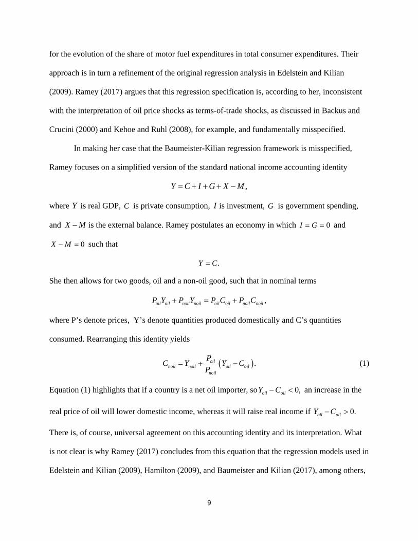
In making her case that the Baumeister-Kilian regression framework is misspecified,
Ramey focuses on a simplified version of the standard national income accounting identity
,Y C I G X M
where Y is real GDP, C is private consumption, I is investment, G is government spending,
and X M is the external balance. Ramey postulates an economy in which 0I G and
0X M such that
.Y C
She then allows for two goods, oil and a non-oil good, such that in nominal terms
,oil oil noil noil oil oil noil noilP Y P Y P C P C
where P’s denote prices, Y’s denote quantities produced domestically and C’s quantities
consumed. Rearranging this identity yields
.oilnoil noil oil oil
noil
PC Y Y C
P (1)
Equation (1) highlights that if a country is a net oil importer, so 0,oil oilY C an increase in the
real price of oil will lower domestic income, whereas it will raise real income if 0.oil oilY C
There is, of course, universal agreement on this accounting identity and its interpretation. What
is not clear is why Ramey (2017) concludes from this equation that the regression models used in
Edelstein and Kilian (2009), Hamilton (2009), and Baumeister and Kilian (2017), among others,

10
are fundamentally misspecified and make no economic sense. The remainder of this section
seeks to clarify the merits of this claim.
Equation (1) suggests a tight relationship between non-oil consumption and net oil
imports. It should be noted, however, that, in a more realistic model, that relationship is not
clear-cut at all. If we allow for nonresidential investment expenditures in this accounting
identity, for example, it becomes indeterminate by how much non-oil consumer expenditures and
by how much business investment expenditures must fall to accommodate the loss in real income
experienced by a net oil-importing economy. This means that the argument outlined by Ramey is
incomplete. We need to specify a mechanism to explain by how much non-oil consumer
expenditures in this economy are affected by this terms-of-trade shock. Edelstein and Kilian
(2009) propose such a mechanism, consisting of four elements:
1. As the real price of crude oil increases, so does the real price of gasoline. The extent
of this price increase depends on the cost share of crude oil in producing gasoline.
2. Because the demand for gasoline is price inelastic, consumers spend more on gasoline
than before the gasoline price increase.
3. To the extent that the revenue from gasoline sales is transferred abroad and not
returned to the U.S. economy, consumers’ aggregate discretionary income (defined as
after-tax real income minus real gasoline expenditures) falls, resulting in lower
domestic aggregate demand.
4. In a Keynesian model, this reduction in aggregate demand may cause a decline in real
GDP.
It is important to stress that the extent to which discretionary income falls depends on the extent
to which the economy relies on net imports of crude oil. If the economy were self-sufficient in

11
crude oil, for example, there would be no change in consumers’ aggregate discretionary income.
Ramey (2017) suggests that the mechanism described by Edelstein and Kilian (2009) implies
that any fall in relative prices would cause a consumption stimulus, as long as demand is
inelastic. Her interpretation, however, is missing Edelstein and Kilian’s point that a discretionary
income effect arises only to the extent that the real gasoline expenditures are transferred abroad
and are not returned to the U.S. economy in the form of higher U.S. exports.
Next, we elaborate on a number of special cases of equation (1). It is useful to start the
discussion with the case of a country that does not produce any crude oil domestically. All oil is
imported. The situation of a country that produces crude oil domestically in addition to importing
crude oil is discussed in sections 3.2 and 3.3.
3.1. Case 1: The Baseline Model without Domestic Oil Production
In the absence of domestic oil production, equation (1) simplifies to
,oilnoil noil oil
noil
PC Y C
P (1 )
where oil noilP P may also be viewed as the terms of trade because oil is the import good and the
non-oil good is the export good. In other words, an increase in the price of oil expressed in units
of the non-oil consumption good, all else equal, reduces the amount of the non-oil consumption
good available for domestic consumption, because more of this good must be used to pay for the
crude oil imports. Equivalently, we may write equation (1 ) as ,noil noil oil oil noilY C P C P
highlighting the fact that crude oil imports must be financed by a trade surplus in the non-oil
consumption good. This case is typical for many oil-importing countries. It also provides a
useful starting point for our discussion.
12
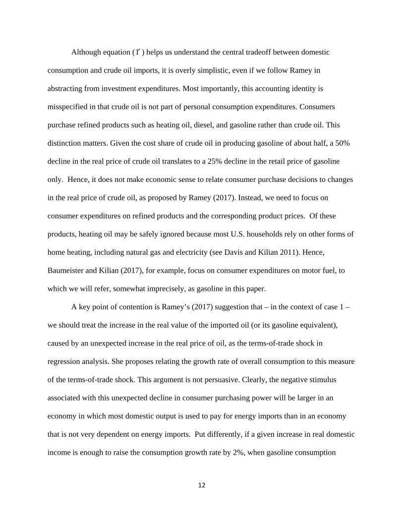
Although equation (1 ) helps us understand the central tradeoff between domestic
consumption and crude oil imports, it is overly simplistic, even if we follow Ramey in
abstracting from investment expenditures. Most importantly, this accounting identity is
misspecified in that crude oil is not part of personal consumption expenditures. Consumers
purchase refined products such as heating oil, diesel, and gasoline rather than crude oil. This
distinction matters. Given the cost share of crude oil in producing gasoline of about half, a 50%
decline in the real price of crude oil translates to a 25% decline in the retail price of gasoline
only. Hence, it does not make economic sense to relate consumer purchase decisions to changes
in the real price of crude oil, as proposed by Ramey (2017). Instead, we need to focus on
consumer expenditures on refined products and the corresponding product prices. Of these
products, heating oil may be safely ignored because most U.S. households rely on other forms of
home heating, including natural gas and electricity (see Davis and Kilian 2011). Hence,
Baumeister and Kilian (2017), for example, focus on consumer expenditures on motor fuel, to
which we will refer, somewhat imprecisely, as gasoline in this paper.
A key point of contention is Ramey’s (2017) suggestion that – in the context of case 1 –
we should treat the increase in the real value of the imported oil (or its gasoline equivalent),
caused by an unexpected increase in the real price of oil, as the terms-of-trade shock in
regression analysis. She proposes relating the growth rate of overall consumption to this measure
of the terms-of-trade shock. This argument is not persuasive. Clearly, the negative stimulus
associated with this unexpected decline in consumer purchasing power will be larger in an
economy in which most domestic output is used to pay for energy imports than in an economy
that is not very dependent on energy imports. Put differently, if a given increase in real domestic
income is enough to raise the consumption growth rate by 2%, when gasoline consumption

13
amounts to 50% of total consumption, one would not expect the same stimulus of 2%, when
gasoline consumption amounts only to 1% of total consumption. Thus, it is essential that we
normalize the real gasoline price shock, before fitting regression models. A formal derivation of
this point is discussed in section 3.5.
Based on the work of Edelstein and Kilian (2009), we can address this concern by
measuring the increase in consumer purchasing power arising from lower gasoline prices by
1 1gas gas PCE gas gas PCEt t t t t t
ngas ngas PCEt t t
C P P C P P
C P P
, (2)
where gas gas PCEt t tC P P denotes the real cost of purchasing gas
tC in period t at the old gasoline
price ,gastP 1 1
gas gas PCEt t tC P P denotes the real cost of purchasing gas
tC in the following period at the
new gasoline price 1 ,gastP and ngas ngas PCE
t t tC P P denotes the real cost of purchasing the non-
gasoline consumption good, all expressed in units of the domestic consumer basket, valued at
.PCEtP 6 The central idea of Edelstein and Kilian (2009) is that we need to focus on the change in
the real price of gasoline triggered by the shock to the real price of imported crude oil in
quantifying the effects of this terms-of-trade shock on private consumption. Equation (2)
expresses the change in real expenditures on oil imports (expressed as their gasoline equivalent)
as a fraction of real expenditures on the non-gasoline consumer good. Multiplying this
expression by gas gast tP P and rearranging yields
1 1 ,gas gas gas PCE gas PCEt t t t t t
ngas ngas gas PCEt t t t
C P P P P P
C P P P
which can be approximated by
6 Note that Edelstein and Kilian (2009) deflate all nominal prices by the overall consumer price index rather than the price index of the non-gasoline consumption good. Given the small expenditure share of gasoline, this difference is immaterial in practice.

14
1 1 ,gas gas gas PCE gas PCEt t t t t t
PCE gas PCEt t t t
C P P P P P
C P P P
given that the share of gasoline in total consumer expenditures is small. In other words, the
change in consumer purchasing power (or discretionary income), denoted by tPP , that is
associated with the terms-of-trade shock approximately equals the percent change in the real
price of gasoline weighted by the nominal share of gasoline expenditures in total consumer
expenditures.7 By construction, 0,tPP if the real price of gasoline rises unexpectedly, and
0,tPP if the real price of gasoline falls unexpectedly. Under the additional empirically
supported assumption that consumers employ a no-change forecast of the real price of gasoline,
tPP may be viewed as a shock to discretionary income or, equivalently, to consumers’
purchasing power (see, e.g., Anderson et al. (2013); Baumeister and Kilian (2016, 2017)). Given
the evidence in Kilian and Vega (2011), we impose the identifying assumption that tPP is
predetermined with respect to the U.S. economy. As shown in Baumeister and Kilian (2017), this
allows one to consistently estimate the cumulative effects of purchasing power shocks from the
stationary regression model
6 6
1 0,t i t i i t i t
i i
c c PP u
(3)
where tu denotes the regression error and tc the percentage growth rate of U.S. real private
consumption. Thus, far from ignoring the role of oil imports and gasoline imports, this
specification is consistent with a world in which all oil is imported. This is not the only
interpretation of this regression model, however, as shown next.
7 In applied work, it is common to approximate the gasoline expenditure share not by the share at the end of the month preceding the real gasoline price change, but rather by the average gasoline expenditure share in the current month.

15
3.2. Case 2: A Model with a Constant Share of Domestic Oil Production in Oil
Consumption
Having discussed the special case of an economy without domestic oil production, we now turn
to the more general case in which some crude oil is produced domestically and some is imported.
Recall that in this case
.oilnoil noil oil oil
noil
PC Y Y C
P (1)
Equivalently, we may write that noil noil oil oil oil noilY C P Y C P such that net oil imports must
be financed by a trade surplus in the non-oil good. In the case of the United States, oil oilC Y and
the oil trade balance is negative. It is useful to first consider the case of a constant oil import
share. For expository purposes, suppose that every period, half of the crude oil consumed by the
economy is produced domestically and the other half is imported. In that case 0.5 ,oil oilY C and
we can write
0.5 .oilnoil noil oil
noil
PC Y C
P (1 )
It may seem that regression model (3) would be invalidated by this change in assumptions, but
this is not the case. The key difference, after expressing this model equivalently in terms of
gasoline prices and quantities, is that the change in purchasing power now depends only on 50%
of real gasoline consumption:
1 10.5 0.5 .gas gas PCE gas gas PCEt t t t t t
ngas ngas PCEt t t
C P P C P P
C P P
( 2 )
As a result, the change in purchasing power now is only half as large as before:
1 10.5 .gas gas gas PCE gas PCEt t t t t t
PCE gas PCEt t t t
C P P P P P
C P P P
16
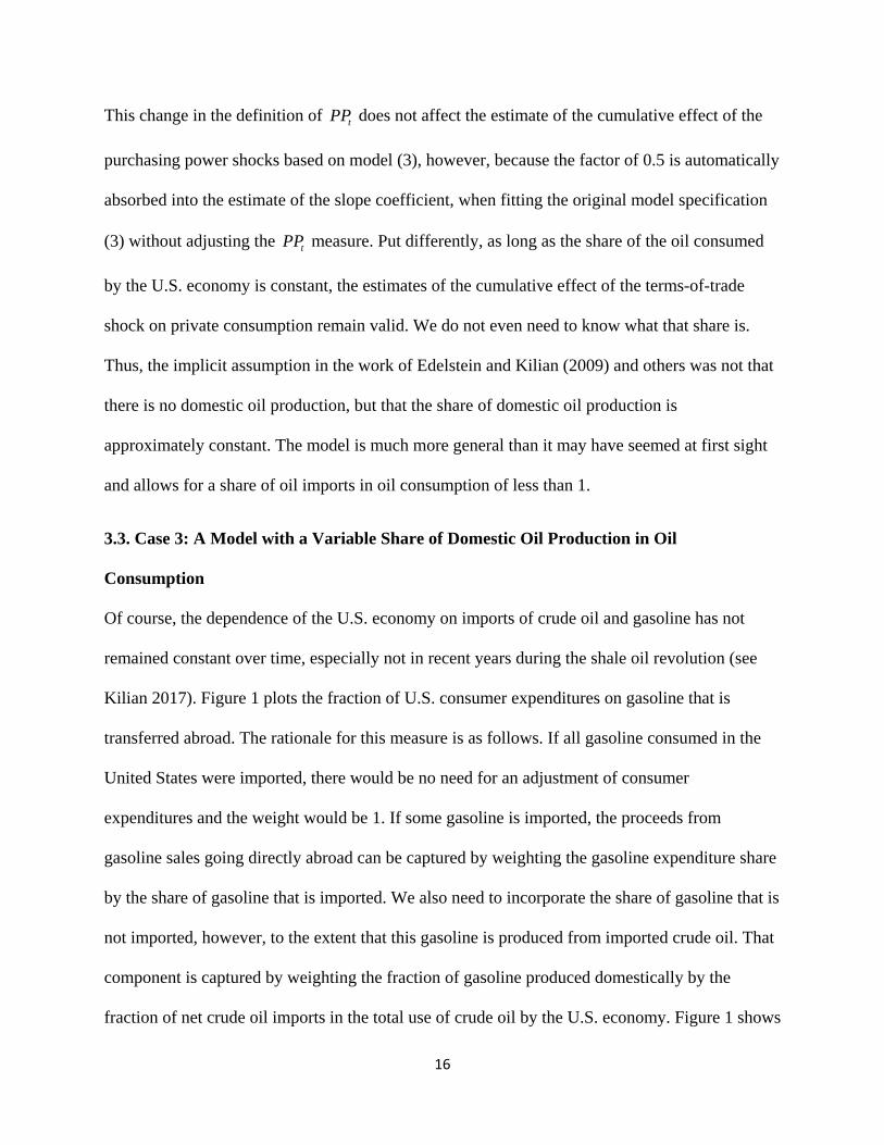
This change in the definition of tPP does not affect the estimate of the cumulative effect of the
purchasing power shocks based on model (3), however, because the factor of 0.5 is automatically
absorbed into the estimate of the slope coefficient, when fitting the original model specification
(3) without adjusting the tPP measure. Put differently, as long as the share of the oil consumed
by the U.S. economy is constant, the estimates of the cumulative effect of the terms-of-trade
shock on private consumption remain valid. We do not even need to know what that share is.
Thus, the implicit assumption in the work of Edelstein and Kilian (2009) and others was not that
there is no domestic oil production, but that the share of domestic oil production is
approximately constant. The model is much more general than it may have seemed at first sight
and allows for a share of oil imports in oil consumption of less than 1.
3.3. Case 3: A Model with a Variable Share of Domestic Oil Production in Oil
Consumption
Of course, the dependence of the U.S. economy on imports of crude oil and gasoline has not
remained constant over time, especially not in recent years during the shale oil revolution (see
Kilian 2017). Figure 1 plots the fraction of U.S. consumer expenditures on gasoline that is
transferred abroad. The rationale for this measure is as follows. If all gasoline consumed in the
United States were imported, there would be no need for an adjustment of consumer
expenditures and the weight would be 1. If some gasoline is imported, the proceeds from
gasoline sales going directly abroad can be captured by weighting the gasoline expenditure share
by the share of gasoline that is imported. We also need to incorporate the share of gasoline that is
not imported, however, to the extent that this gasoline is produced from imported crude oil. That
component is captured by weighting the fraction of gasoline produced domestically by the
fraction of net crude oil imports in the total use of crude oil by the U.S. economy. Figure 1 shows

17
the sum of these two components, expressed as a percentage of consumer expenditures on
gasoline.
Figure 1 shows that this import dependence measure generally increases, as the price of
oil rises, and decreases, as the price of oil falls. The average share is 49%, but at times the share
dropped to 25% or reached 70%. To the extent that this share at a given point in time is above or
below the average share of 49%, one would expect the regression model (3) to overpredict or
underpredict the cumulative effects of terms-of-trade shocks associated with oil price
fluctuations. This point has indeed been ignored in the existing literature or has been thought to
be of secondary importance. As a result of the fluctuations in this share, one would expect
regression model (3) to be reasonably accurate only during periods when the share of domestic
oil production in the use of oil is close to its long-run average. That was indeed the argument
made by Baumeister and Kilian (2017) in defense of their original approach to modelling the
2014Q3-2016Q1 episode. That study observed that in mid-2014 the share of domestic oil
production was close to its long-run average of 49%, suggesting that the estimates of model (3)
should be useful in analyzing this episode. In contrast, for the episode of the 1986 oil price
decline, this assumption is invalid because at that point in time the share was only 34% (see
Figure 1).
One way of handling this concern would be the use of time-varying coefficient regression
models, but such models are prone to overfitting and their estimates can be sensitive to the
choice of Bayesian priors. As shown by Baumeister and Kilian (2017), an alternative and more
direct way of quantifying the importance of changes in the dependence of the U.S. economy on
oil and gasoline imports is to directly incorporate this evolution in the construction of the
purchasing power shock. A simple approximation is to weight U.S. consumer expenditures on

18
gasoline by the share of the proceeds going abroad, resulting in an alternative definition of
purchasing power shocks,
1 1 (1 ) ,gas gas gas PCE gas PCE
gasoline imports gasoline imports net oil importst t t t t tt t tPCE gas PCE
t t t t
C P P P P Ps s s
C P P P
where gasoline importsts is the seasonally adjusted share of U.S. motor gasoline imports in total U.S.
motor gasoline consumption, as reported by the U.S. Energy Information Administration, and
where net oil importsts is the seasonally adjusted share of U.S. net crude oil imports in the total use of
crude oil by the U.S. economy, as defined in Kilian (2017). The adjustment factor by which we
multiply the original tPP measure corresponds to the share shown in Figure 1. This alternative
measure of shocks to consumer’s purchasing power (or discretionary income), denoted by
,alternativetPP is not only more relevant for understanding the dependence of U.S. consumers on
imports of crude oil and gasoline than the share of net imports in petroleum products supplied, as
reported by Ramey (2017), but it also avoids the ad hoc aggregation of crude oil and refined
products. It should be kept in mind, however, that even alternativetPP is only an approximation,
because it ignores changes in oil and gasoline inventories, because it assumes that the net share
of imported crude oil is the same in the production of all refined products, because it does not
differentiate between gasoline and other motor fuel, and because it makes no allowance for
changes over time in the extent of petrodollar recycling from abroad.
One advantage of this alternative specification is that we can directly evaluate the
empirical content of Ramey’s concern regarding changes in the dependence of the U.S. economy
on crude oil imports by comparing the estimates of the discretionary income effect based on
baseline specification (3) with the estimates based on the alternative specification
19
6 6
1 0,alternative
t i t i i t i ti i
c c PP u
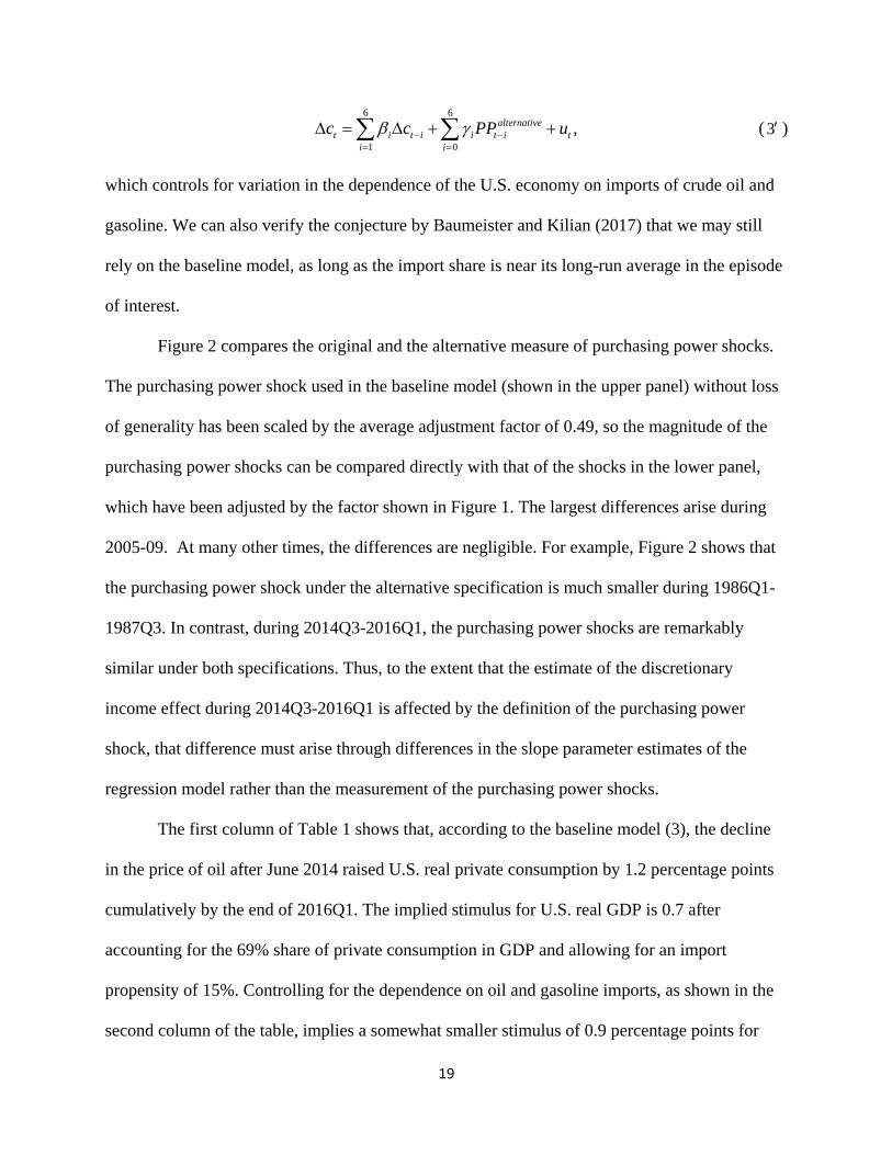
( 3 )
which controls for variation in the dependence of the U.S. economy on imports of crude oil and
gasoline. We can also verify the conjecture by Baumeister and Kilian (2017) that we may still
rely on the baseline model, as long as the import share is near its long-run average in the episode
of interest.
Figure 2 compares the original and the alternative measure of purchasing power shocks.
The purchasing power shock used in the baseline model (shown in the upper panel) without loss
of generality has been scaled by the average adjustment factor of 0.49, so the magnitude of the
purchasing power shocks can be compared directly with that of the shocks in the lower panel,
which have been adjusted by the factor shown in Figure 1. The largest differences arise during
2005-09. At many other times, the differences are negligible. For example, Figure 2 shows that
the purchasing power shock under the alternative specification is much smaller during 1986Q1-
1987Q3. In contrast, during 2014Q3-2016Q1, the purchasing power shocks are remarkably
similar under both specifications. Thus, to the extent that the estimate of the discretionary
income effect during 2014Q3-2016Q1 is affected by the definition of the purchasing power
shock, that difference must arise through differences in the slope parameter estimates of the
regression model rather than the measurement of the purchasing power shocks.
The first column of Table 1 shows that, according to the baseline model (3), the decline
in the price of oil after June 2014 raised U.S. real private consumption by 1.2 percentage points
cumulatively by the end of 2016Q1. The implied stimulus for U.S. real GDP is 0.7 after
accounting for the 69% share of private consumption in GDP and allowing for an import
propensity of 15%. Controlling for the dependence on oil and gasoline imports, as shown in the
second column of the table, implies a somewhat smaller stimulus of 0.9 percentage points for
20
consumption (or 0.5 percentage points for real GDP).8 Nevertheless, the estimates are in the
same ballpark. In both cases, there is clear evidence of a modest stimulus associated with the
discretionary income effect. As expected, controlling for the dependence on oil and gasoline
imports changes the estimates without overturning the substantive conclusions based on model
(3).
From a policy point of view, the difference between a stimulus of 0.7 percentage points
for U.S. real GDP and a stimulus of 0.5 percentage points is negligible. Thus, Ramey’s
conjecture that the baseline results in Baumeister and Kilian (2017) are an artifact of their failure
to model time variation in the dependence of the U.S. economy on imports of gasoline and crude
oil is clearly rejected. We conclude that, on a priori grounds, the alternative specification (3 )
proposed by Baumeister and Kilian (2017) may be more appealing, but that the two
specifications generate similar results for the 2014-16 episode, contradicting Ramey’s claim.
Moreover, which specification is used does not affect the substantive conclusion in Baumeister
and Kilian (2017) that the net stimulus for the U.S. economy implied by lower oil prices after
June 2014 has been close to zero.
In the last two columns of Table 1 we repeat this exercise for the 1986-87 episode, which
was characterized by a similar, if much smaller sustained decline in the real price of oil. For this
episode, one would expect the baseline model to be less accurate, given that the economy was
less dependent on oil and gasoline imports in 1985Q4 than in 2014Q2, as reflected in the
alternative purchasing power measure in Figure 2. The baseline model (3) implies that, in the
seven quarters following 1985Q4, U.S. real private consumption cumulatively increased by 0.8
8 The estimates in Table 1 for the alternative model do not match those in Baumeister and Kilian (2017) exactly due to a data transcription error in that paper, which has been corrected in the current analysis. For example, the cumulative effect on consumption in model ( 3 ) is 0.87 rather than 0.92, as reported in Baumeister and Kilian (2017).

21
percentage points, as a result of the decline in the real price of oil that started in early 1986,
implying a stimulus of 0.5 percentage points for real GDP. In contrast, the alternative model
( 3 ) suggests a cumulative increase in private consumption of only 0.4 percentage points and an
implied stimulus for U.S. real GDP of only 0.2 percentage points (see Table 1). Although this
difference is not much larger in absolute terms than in the 2014-16 episode, it is at least twice as
large in relative terms. This example illustrates that the adjustment factor may matter, providing
empirical support for Baumeister and Kilian’s decision to model the 1986-87 episode based on
model (3 ) rather than (3).
3.4. Yet Another Definition of the Purchasing Power Shock?
Given Ramey’s insistence that the approach described in sections 3.2 and 3.3 is at odds with the
policy consensus, it is useful to relate our approach to the definition of purchasing power shocks
used in Council of Economic Advisers (2014, p. 25):
1(1 ) ,oil oil
t tt oil
t
P Pas a s
P
where ( ) ( ) ,oil oil oil Yt t t t t ts M X P Y P s is the sample average of ,ts ( )oil oil oil
t t tM X P denotes
nominal net oil imports, tY is real GDP, and YtP is the GDP deflator.9 The parameter a is either
0 or 1. For 0,a the Council of Economic Advisers measure of the purchasing power shock
reduces to
1 ,oil oil
t toil
t
P Ps
P
9 To be precise, the Council of Economic Advisers (2014) works with net petroleum imports rather than net crude oil imports, where petroleum is defined as crude oil plus selected refined products, but it weights the nominal expenditure share for petroleum by the change in the price of crude oil. Thus, for expository purposes, it is preferable to treat the quantities of oil and gasoline as exchangeable and to denote net petroleum imports as net oil imports.

22
and for 1,a it reduces to
1 .oil oil
t tt oil
t
P Ps
P
It can be shown that these definitions under suitable simplifying assumptions may be derived
from the original and the alternative definition of the purchasing power shock, respectively, as
discussed in sections 3.2 and 3.3. For expository purposes, we consider the case of 1.a Recall
our alternative definition of the purchasing power shock as
1 1 (1 ) ,gas gas gas PCE gas PCE
gasoline imports gasoline imports net oil importst t t t t tt t tPCE gas PCE
t t t t
C P P P P Ps s s
C P P P
where ( ) ,net oil imports oil oil oil oil oil oil oilt t t t t t t ts M X P Y M X P and suppose that ,t tC Y which
amounts to imposing that 0,I G X M as in Ramey’s analysis. Further suppose that
gasoline and oil are the same good such that 0,gasoline importsts ,gas oil
t tP P and ,gas oilt tC C and
suppose that there is no inflation, so the real and the nominal price of oil coincide. Finally
suppose that the change in U.S. oil inventories is zero such that oil oil oil oilt t t tC Y M X (see
Kilian 2017). Then simple substitution shows that the alternative purchasing power shock
measure reduces to
1 ,oil oil oiloil oil oil oilt t tt t t t
Y oil oil oilt t t t t
M X PC P P P
Y P P C P
or, equivalently,
1 ,oil oil oil oil oilt t t t t
Y oilt t t
M X P P P
Y P P
which up to the sign normalization is identical to the definition used by the Council of Economic
Advisers (2014, 2016). Of course, there is no good reason for using any of these unnecessary

23
simplifying assumptions, but this exercise illustrates that policymakers fully understand the need
for normalizing by the expenditure share, directly refuting Ramey’s (2017) claim in this regard.
This discussion also helps explain why the approximate results reported in Council of Economic
Advisers (2016), as discussed in section 5, are close to those in Baumeister and Kilian (2017).
The reason is that both use fundamentally the same approach, except that the computations in
Baumeister and Kilian (2017) are more precise.
3.5. What Is the Economic Rationale for Weighting Real Gasoline Price Shocks by the
Gasoline Expenditure Share?
In subsection 3.1, we explained intuitively why shocks to the real price of gasoline must be
weighted by the gasoline expenditure share of consumers, when quantifying the discretionary
income effect. Ramey (2017) makes the case that this approach is not supported by economic
theory. She insinuates that fully specified economic models of the transmission of oil price
shocks imply that the response of private consumption does not depend on consumers’ energy
share, rendering standard regression estimates of the discretionary income effect invalid.
This claim is not correct. Even granting that none of the currently available DSGE
models provides a satisfactory representation of the real world, as noted by Kilian (2014), and
that their quantitative implications are sensitive to ad hoc modelling assumptions, the fact that
the impact of energy price shocks on the economy depends on the share of firm and household
energy expenditures is well established. In fact, declines in the share of energy in production and
consumption have been held responsible by many researchers for the reduced overall effect of oil
price shocks on the U.S. economy in the literature (see, e.g., Edelstein and Kilian (2009),
Blanchard and Galí (2010), Kilian and Vigfusson (2017)). The same point was made by Yellen
(2011), as discussed earlier.

24
It is useful to review the theoretical rationale for the approach described in the preceding
subsections. The DSGE model of Backus and Crucini (2000) referred to by Ramey is not helpful
in answering that question because, in that model, households do not directly consume energy.
Oil enters only into the production function. That assumption is typical for much of the DSGE
literature on the transmission of oil price shocks, but fails to capture the reality that consumer
spending on motor fuel is a major channel of the transmission of oil price shocks (see, e.g.,
Leduc and Sill 2004). In more recent DSGE models such as Dhawan and Jeske (2008a,b), which
explicitly allow for household energy consumption, however, the responses of output to an
exogenous real energy price shock depend on the household energy share. The economic
rationale for weighting real gasoline price shocks is perhaps best illustrated by the New
Keynesian DSGE model described in Blanchard and Galí (2010), which allows oil to enter both
the utility function and the production function. The model makes no distinction between crude
oil and gasoline. Blanchard and Galí (2010, p. 418) show that, in equilibrium, the relationship
between real private consumption and real value added in an oil-importing economy is
approximately
log log log ,1
oil oil oilt t t
t t CPI PPIt t t
C P PC Y
C P P
where tC is real private consumption, tY is real value added, is the oil share in production,
oil oil CPIt t t tC P C P is the oil expenditure share of consumers, and oil PPI
t tP P is the real price of oil.
This expression may be viewed as a generalization of equation (1). Given that is quite small
and that there is little difference between the PPI and the CPI, this expression can be
approximated by
25
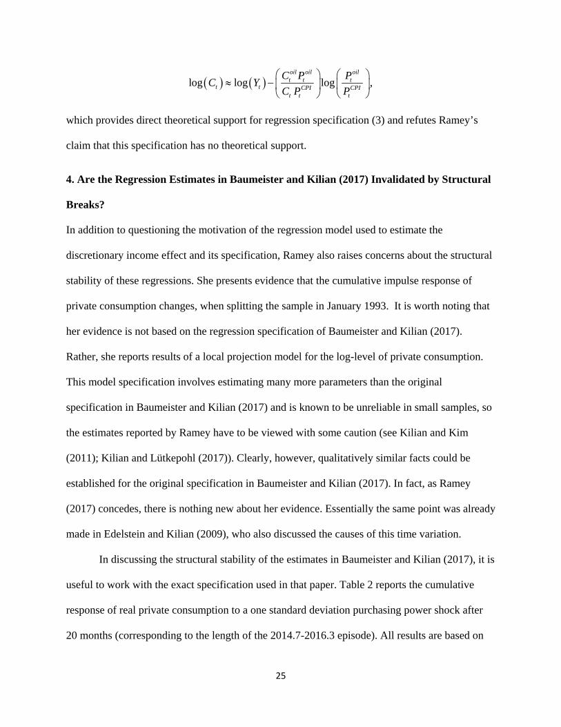
log log log ,oil oil oilt t t
t t CPI CPIt t t
C P PC Y
C P P
which provides direct theoretical support for regression specification (3) and refutes Ramey’s
claim that this specification has no theoretical support.
4. Are the Regression Estimates in Baumeister and Kilian (2017) Invalidated by Structural
Breaks?
In addition to questioning the motivation of the regression model used to estimate the
discretionary income effect and its specification, Ramey also raises concerns about the structural
stability of these regressions. She presents evidence that the cumulative impulse response of
private consumption changes, when splitting the sample in January 1993. It is worth noting that
her evidence is not based on the regression specification of Baumeister and Kilian (2017).
Rather, she reports results of a local projection model for the log-level of private consumption.
This model specification involves estimating many more parameters than the original
specification in Baumeister and Kilian (2017) and is known to be unreliable in small samples, so
the estimates reported by Ramey have to be viewed with some caution (see Kilian and Kim
(2011); Kilian and Lütkepohl (2017)). Clearly, however, qualitatively similar facts could be
established for the original specification in Baumeister and Kilian (2017). In fact, as Ramey
(2017) concedes, there is nothing new about her evidence. Essentially the same point was already
made in Edelstein and Kilian (2009), who also discussed the causes of this time variation.
In discussing the structural stability of the estimates in Baumeister and Kilian (2017), it is
useful to work with the exact specification used in that paper. Table 2 reports the cumulative
response of real private consumption to a one standard deviation purchasing power shock after
20 months (corresponding to the length of the 2014.7-2016.3 episode). All results are based on

26
the baseline model (3). The first row shows the full-sample estimate implied by this model. The
next two rows in the table report the corresponding estimates for the two subperiods considered
by Ramey (2017). Table 2 shows that the estimate based on the subsample 1970.2-1992.12 is 3.4
times larger than the estimate based on the subsample 1993.1-2016.3.
The difference across subsamples is not nearly as large as implied by the inefficient local
projection estimator employed in Ramey (2017), but still large. It is also irrelevant for Ramey’s
argument that the estimates in Baumeister and Kilian (2017) are misleading. If there were a
structural change, as asserted by Ramey, the analysis in Baumeister and Kilian (2017) would be
in error to the extent that the full-sample estimate (which Ramey did not report) differs from the
estimate based on the second subsample. The value of the response estimate for the first
subsample is irrelevant for that question. Table 2 shows that the full-sample estimate of 0.12 is
not much larger than the estimate of 0.07 for the second subsample. It is this much more modest
difference in estimates that requires an economic explanation.
This difference may still seem too large for comfort, but what Ramey fails to mention is
that there are well-known reasons for the apparent instability in the regression coefficients, when
the model is evaluated on subsamples. Such instability is in fact expected based on previous
research, even in the absence of any structural breaks in the data-generating process. Although
the average responses of real consumption to purchasing power shocks may be estimated reliably
using long enough samples, when considering short subsamples, these responses will change in
magnitude and even in sign, as the composition of oil demand and oil supply shocks evolves
over time, giving the mistaken appearance of structural instability, even when there is no
structural change at all (see, e.g., Kilian (2008; 2009a,b); Kilian and Park (2009)). For example,
as discussed in Edelstein and Kilian (2009), the real gasoline price in the second half of Ramey’s

27
sample is dominated by unexpected shifts in the flow demand for crude oil, which cushion the
direct effect of oil price fluctuations on the U.S. economy. Thus, there is no mystery as to why
the response estimates are much lower in the second half of the sample. This result simply
reflects changes in the composition of oil demand and oil supply shocks.
This point may be illustrated empirically. The second subsample chosen by Ramey is
known to include few important supply and storage demand shocks. Instead, it is dominated by
flow demand shocks for oil, making it unrepresentative for the sample as a whole as well as for
the period since June 2014 (see, e.g., Kilian and Murphy 2014). By slightly extending the second
subsample to include the invasion of Kuwait in 1990, which constitutes an important shock to oil
supply and to the storage demand for oil, the estimate for the second subsample increases from
0.0692 to 0.0997. The latter estimate is very close to the full-sample estimate of 0.1194 (see
Table 2), suggesting that there is no instability at all. In fact, using model estimates based on the
full sample, as in Baumeister and Kilian (2017), makes sense in analyzing the effects of the
2014-16 oil price decline, because the real price of oil during that episode was driven by a
combination of different demand and supply shocks rather than primarily by flow demand
shocks (see Baumeister and Kilian (2016); Kilian (2017)).
It is conceivable, of course, that there are other reasons for the decline in the response of
private consumption that are unrelated to changes in the composition of oil demand and oil
supply shocks. Ramey provides three specific reasons why she believes that the effect of oil and
gasoline price shocks should have declined. First, she suggests that real oil price shocks caused
larger overall terms-of-trade fluctuations in the 1970s and early 1980s than in recent years. This
argument is missing the point. First, Ramey misrepresents Backus and Crucini’s (2000) work.
There are no exogenous real oil price shocks in their model, so Backus and Crucini could not
28
possibly have quantified the causal effects of real oil price shocks. What they actually showed
was that the time variation in the dynamic correlation between the real price of oil and the U.S.
terms of trade reflects changes in the composition of oil demand and oil supply shocks. In their
words:
“… since our dynamic general equilibrium model predicts that the economy responds differently to oil supply shocks than to other shocks, changes in their relative importance help to account for the unstable correlations in the data” (p. 185).
This point and its implications have already been addressed in our earlier discussion. Second,
there is no a priori presumption that the real price of oil and the overall terms of trade of the U.S.
economy should move proportionately. Clearly, the terms of trade are subject to many more
shocks than real oil price shocks, so the weakening unconditional co-movement between the real
price of oil and the overall U.S. terms of trade, as displayed in Figure 1 of Ramey (2017), is not
evidence of a structural change in the data-generating process.
Second, Ramey insists that the terms of trade are affected by U.S. gasoline price controls
and rationing. She proposes scaling the nominal gasoline price underlying the regressions in
Baumeister and Kilian (2017) by a multiplicative factor as used in Ramey and Vine (2011). This
adjustment is intended to capture the cost to consumers of waiting at gas stations, which arose
during 1973.12-1974.5 and in 1979.5-1979.7, when the government imposed gasoline price
ceilings in response to oil price increases. Because this waiting cost is not associated with a
transfer of real income abroad, however, this adjustment must not be used in quantifying the
discretionary income effect. This misunderstanding is closely related to Ramey’s failure to
appreciate that purchasing power shocks reflect real income transfers abroad.
Finally, Ramey argues that declines in the share of oil imports explain the smaller
cumulative response of private consumption in the sample starting in January 1993. That

29
argument was already dispensed with in section 3, where we showed that the response of private
consumption in 2014-16 is quite similar, whether we allow for changes in the dependence on oil
and gasoline imports or not. Likewise, Baumeister and Kilian (2017) stressed that their
substantive conclusions are unaffected by this adjustment. Thus, the evidence and arguments in
Ramey (2017) regarding potential structural instabilities in the regression model of Baumeister
and Kilian (2017) are missing the point.
5. Whither Regression Analysis?
As stressed by Ramey (2017), the estimates in Baumeister and Kilian (2017) are very close to the
“direct effects” of lower oil prices on U.S. real GDP growth reported in the 2016 Economic
Report to the President (Council of Economics Advisers (2016), Box 2-1, p. 55-58) based on a
simple back-of-the-envelope calculation. This report argued that if one values all U.S. net
imports of crude oil and petroleum products at the nominal price of crude oil, then, given the
cumulative decline in this price since June 2014, all else equal, we would expect a 0.1% increase
in U.S. real GDP in 2014 and an additional increase of 0.2% in 2015. The implied cumulative
increase in real GDP after mid-2014 is about 0.3%, which is remarkably close to the net stimulus
of 0.39% estimated in Baumeister and Kilian (2017). Likewise, for private consumption the
estimate of 0.6 in the Report is close to the estimate of 0.7 in Baumeister and Kilian.
The overall tenor of Ramey’s analysis is that the effects of unexpectedly lower oil prices
on consumption should be systematically smaller than the estimates reported in Baumeister and
Kilian (2017), yet at the same time she is forced to acknowledge that these estimates are similar
to those obtained in the Report, which she considers correctly executed. Our analysis suggests
that it is not an accident that the Report reaches conclusions similar to Baumeister and Kilian
(2017). As shown in section 3.4, both studies measure purchasing power shocks in
30
fundamentally the same way, the only difference being that Baumeister and Kilian (2017)
dispense with the restrictive assumptions underlying the analysis in the Report.
This is not the only difference, however. The Report is careful to stress that care is
required in interpreting its estimate of the “direct effect,” because “consumers for whom lower
gasoline prices freed up income for other purchases … may take time … to make additional
purchases, so the timing of the additional spending may lag the declines in oil prices” (p. 56).
Nor do the estimates in the Report account for additional multiplier effects from changes in
spending (p. 56). Thus, these direct estimates conceptually differ from the cumulative effect
estimated by Baumeister and Kilian (2017). Unlike the estimates cited in the Report, Baumeister
and Kilian’s (2017) estimates account for typical delays in spending as well as multiplier effects.
Perhaps most importantly, the analysis in Baumeister and Kilian (2017) explicitly
recognizes the fact that consumer responses depend on the real price of gasoline rather than on
the real price of oil, and it accounts for the timing and persistence of changes in the real price of
gasoline on a month-by-month basis, allowing more accurate estimates of the cumulative effects
and providing more information about the evolution of these cumulative effects month by month.
Their analysis also dispenses with a number of other simplifying assumptions, as discussed in
section 3.4. Thus, the fact that the back-of-the-envelope estimates in the Report are in the same
ballpark as those in Baumeister and Kilian (2017) was by no means obvious ex ante. Back-of-
the-envelope computations of this type are best viewed as a preliminary approximation to be
validated by more formal regression-based methods of the type discussed in this paper rather
than as a substitute for more formal analysis.
6. Conclusion
The discretionary income effect is a central element of the transmission of oil price shocks, as
31
discussed in the existing literature. Recently, Ramey (2017) has suggested that empirical studies
quantifying this effect such as Edelstein and Kilian (2009), Hamilton (2009, 2013), and
Baumeister and Kilian (2017), among others, have no economic foundation. She not only
disputed the very existence of a discretionary income effect, but she called into question the
stability of commonly used regression models in this literature, and she even questioned the data
used by these models. Ramey’s critique is remarkable in that she does not provide any
constructive alternative modeling approaches, but implies that regression models are simply not
necessary to assess the questions of interest.
Our analysis showed that Ramey’s central claim that the discretionary income channel
makes no economic sense is mistaken. In fact, the shocks to discretionary income discussed in
the literature (also referred to as purchasing power shocks) are substantively identical to the
shifts in real domestic income associated with a terms-of-trade shock stressed by Ramey. The
specification of conventional regression models of the discretionary income effect is fully
consistent with recent New Keynesian DSGE models of the transmission of oil price shocks.
Moreover, these regression models are already designed to deal with many of the concerns raised
by Ramey. We discussed generalizations of these models and assessed the robustness of standard
specifications to the concerns raised by Ramey.
We also demonstrated that the model specifications and diagnostics used by Ramey to
establish the structural instability of regression models of the transmission of oil shocks are
flawed. We showed that her modelling approach ignores recent developments in the literature,
and we explained why the data modifications proposed by Ramey are inappropriate in the
context of this literature. Finally, we discussed the importance of regression analysis in
quantifying the effects of oil price shocks. We concluded that there is no reason to rewrite the

32
literature on the transmission of oil price shocks.
References:
Anderson, S.T., R. Kellogg, and J.M. Sallee (2013), “What Do Consumers Believe about Future Gasoline Prices,” Journal of Environmental Economics and Management, 66, 383-403. Backus, D.K., and M.J. Crucini (2000), “Oil Prices and the Terms of Trade,” Journal of International Economics, 50(1), 185-213. Baumeister, C., and L. Kilian (2016), “Forty Years of Oil Price Fluctuations: Why the Price of Oil May Still Surprise Us,” Journal of Economic Perspectives, 30, 139-160, Winter. Baumeister, C., and L. Kilian (2017), “Lower Oil Prices and the U.S. Economy: Is This Time Different?”, Brookings Papers on Economic Activity, Fall, 287-336. Bernanke, B.S. (2006), “The Economic Outlook,” Remarks before the National Italian American Foundation, New York, November 28. Blanchard, O.J., and J. Galí (2010), “The macroeconomic effects of oil price shocks: Why Are the 2000s so different from the 1970s?” in: Galí, J., and M. Gertler (eds.), International Dimensions of Monetary Policy, University of Chicago Press: Chicago, IL, 373-421. Coglianese, J, Davis, L.W., Kilian, L., and J.H. Stock (2017), “Anticipation, Tax Avoidance, and the Price Elasticity of Gasoline Demand,” Journal of Applied Econometrics, 32(1), 1-15. Council of Economic Advisers (2014), “The All-of-the-Above Energy Strategy as a Path to Sustainable Economic Growth,” The White House, Office of the Press Secretary, Washington, DC. Council of Economic Advisers (2015), Economic Report of the President, Government Printing Office, Washington, DC. Council of Economic Advisers (2016), Economic Report of the President, Government Printing Office, Washington, DC. Davis, L.W., and L. Kilian (2011), “The Allocative Cost of Price Ceilings in the U.S. Residential Market for Natural Gas,” Journal of Political Economy, 119(2), 212-241. Dhawan, R. and K. Jeske (2008a), “Energy Price Shocks and the Macroeconomy: The Role of Consumer Durables,” Journal of Money, Credit, and Banking, 40, 1357-1377. Dhawan, R. and K. Jeske (2008b), “What Determines the Output Drop after an Energy Price Increase? Household or Firm Energy Share?” Economics Letters, 107, 202-205. Edelstein, P., and L. Kilian (2007), “The Response of Business Fixed Investment to Energy Price

33
Changes: A Test of Some Hypotheses about the Transmission of Energy Price Shocks,” B.E. Journal of Macroeconomics, 7. Edelstein, P., and L. Kilian (2009), “How Sensitive Are Consumer Expenditures to Retail Energy Prices?” Journal of Monetary Economics, 56, 766-779. Fried, E., and C. Schultz (1975), Higher Oil Prices and the World Economy, Brookings Institution, Washington, DC. Hamilton, J.D. (1988), “A Neoclassical Model of Unemployment and the Business Cycle,”
Journal of Political Economy, 96, 593-617. Hamilton, J.D. (2009), “Causes and Consequences of the Oil Shock of 2007-08,” Brookings Papers on Economic Activity, 1, Spring, 215-259. Hamilton, J.D. (2013), “Oil Prices, Exhaustible Resources, and Economic Growth,” in Fouquet, R. (ed.), Handbook of Energy and Climate Change, Cheltenham, U.K.: Edward Elgar Publishing, 29-57. Hamilton, J.D. (2017), Comments on ‘Lower Oil Prices and the U.S. Economy: Is This Time Different?” by Christiane Baumeister and Lutz Kilian,’ Brookings Papers on Economic
Activity, Fall, 337-343. Kehoe, T.J., and K.J. Ruhl (2008), “Are Shocks to the Terms of Trade Shocks to Productivity?” Review of Economic Dynamics, 11, 804-829. Kilian, L. (2008), “The Economic Effects of Energy Price Shocks,” Journal of Economic Literature, 46(4), 871-909. Kilian, L. (2009a), “Not All Oil Price Shocks Are Alike: Disentangling Demand and Supply Shocks in the Crude Oil Market,” American Economic Review, 99(3), 1053-1069. Kilian, L. (2009b), “Comment on ‘Causes and Consequences of the Oil Shock of 2007-08’ by James D. Hamilton,” Brookings Papers on Economic Activity, 1, Spring, 267-278. Kilian, L. (2014), “Oil Price Shocks: Causes and Consequences,” Annual Review of Resource Economics, 6, 133-154. Kilian, L. (2017), “The Impact of the Fracking Boom on Arab Oil Producers,” forthcoming: Energy Journal. Kilian, L., and Y.J. Kim (2011), “How Reliable Are Local Projection Estimators of Impulse Responses?” Review of Economics and Statistics, 93(4), 1460-1466. Kilian, L., and H. Lütkepohl (2017), Structural Vector Autoregressive Analysis, Cambridge University Press, forthcoming.

34
Kilian, L., and D.P. Murphy (2014), “The Role of Inventories and Speculative Trading in the Global Market for Crude Oil,” Journal of Applied Econometrics, 29, 454-478. Kilian, L, and C. Park (2009), “The Impact of Oil Price Shocks on the U.S. Stock Market,” International Economic Review, 50, 1267-1287. Kilian, L., Rebucci, A. and N. Spatafora (2009), “Oil Shocks and External Balances,” Journal of International Economics, 77(2), 181-194. Kilian, L., and C. Vega (2011), “Do Energy Prices Respond to U.S. Macroeconomic News? A Test of the Hypothesis of Predetermined Energy Prices,” Review of Economics and Statistics, 93, 660-671. Kilian, L., and R.J. Vigfusson (2017), “The Role of Oil Price Shocks in Causing U.S. Recessions,” forthcoming: Journal of Money, Credit, and Banking. Leduc, S, and K. Sill (2004), “A Quantitative Analysis of Oil Price Shocks, Systematic Monetary Policy, and Economic Downturns,” Journal of Monetary Economics, 51, 781-808. Ramey, V.A. (2017), Comments on ‘Lower Oil Prices and the U.S. Economy: Is This Time Different?” by Christiane Baumeister and Lutz Kilian,’ Brookings Papers on Economic Activity, Fall, 343-351. Ramey, V.A., and D.J. Vine (2011), “Oil, Automobiles, and the US Economy: How Much Have Things Really Changed?” NBER Macroeconomics Annual, 25, ed. Acemoglu, D., and M. Woodford,.Chicago: University of Chicago Press, 333-368. Sachs, J.D. (1982), “The Oil Shocks and Macroeconomic Adjustment in the United States,”
European Economic Review, 18, 243-248. Yellen, J.L. (2011), “Commodity Prices, the Economic Outlook, and Monetary Policy,” speech at the Economic Club of New York, New York, NY, April 11. Yellen, J.L. (2015), Monetary Policy Report, Board of Governors of the Federal Reserve System.

35
Table 1: Predicted Cumulative Stimulus from Lower Oil Prices on the U.S. Economy
2014.Q3-2016.Q1 1986.Q1-1987.Q3 Baseline
Model (3) Alternative Model (3 )
Baseline Model (3)
Alternative Model (3 )
Effect of Lower Oil Prices on U.S. Real Private Consumption (%)
1.20
0.87
0.84
0.43 Implied Effect on U.S. Real GDP (%)
0.70
0.51
0.45
0.23
Notes: Models (3) and (3 ) are described in the text. The alternative model differs from the baseline model in that it allows for variation in the dependence of the U.S. economy on imports of crude oil and gasoline, as shown in Figure 1. Table 2: Cumulative Response of U.S. Consumption in Month 20 to a One Standard Deviation Purchasing Power Shock
Sample Cumulative Response (Percent) 1970.2-2016.3 (full sample) 0.1194 1970.2-1992.12 (first subsample) 0.2380 1993.1-2016.3 (second subsample) 0.0692 1990.1-2016.3 (including invasion of Kuwait) 0.0997
Notes: All results are based on the baseline model (3).

36
Figure 1: Adjustment Factor for the U.S. Dependence on Gasoline and Crude Oil Imports, 1973.1-2016.3
Notes: Authors’ calculations based on data in the U.S. Energy Information Administration’s Monthly Energy Review, as discussed in the text. This adjustment factor measures the extent to which U.S. consumer gasoline expenditures are transferred abroad. It accounts for time variation in the share of gasoline imports in U.S. gasoline consumption, as well as time variation in the share of U.S. net crude oil imports in the domestic use of crude oil. The underlying data have been seasonally adjusted.
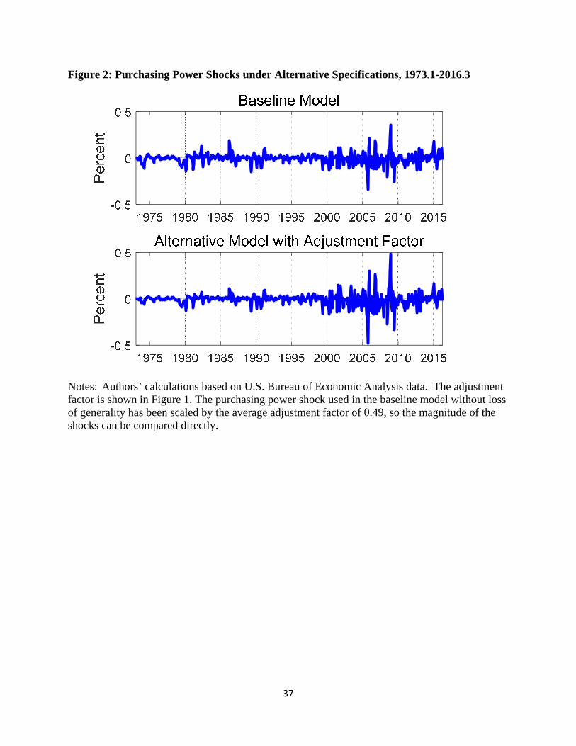
37
Figure 2: Purchasing Power Shocks under Alternative Specifications, 1973.1-2016.3
Notes: Authors’ calculations based on U.S. Bureau of Economic Analysis data. The adjustment factor is shown in Figure 1. The purchasing power shock used in the baseline model without loss of generality has been scaled by the average adjustment factor of 0.49, so the magnitude of the shocks can be compared directly.