is the welding current - cranfield university
TRANSCRIPT

CRANFIELD UNIVERSITY
T.E.B. OGUNBIYI
PROCESS MONITORING AND ADAPTIVE QUALITY CONTROL FOR ROBOTIC GAS METAL
ARC WELDING
School of Industrial and Manufacturing Science
PhD Thesis

CRANFIELD UNIVERSITY
School of Industrial and Manufacturing Science
PhD Thesis
Academic Year 1994-95
T.E.B. OGUNBIYI
PROCESS MONITORING AND ADAPTIVE QUALITY CONTROL FOR ROBOTIC GAS METAL ARC WELDING
Supervisor: John Nonish
June 1995
This thesis is submitted in fulfilment of the requirement for the degree of PhD

ABSTRACT
The aim of this research was to develop an adaptive quality control strategy for robotic gas metal arc welding of thin steel sheets. Statistical methods were used to monitor and control the quality of welds produced.
The quality of welds cannot be directly measured during welding. It can however be estimated by correlating weld quality parameters to relevant process variables. It was found sufficient to do this using welding current and voltage transient signals only.
The strategy developed was problem solving oriented with emphasis on quality assurance, defect detection and prevention. It was based on simple algorithms developed using multiple regression models, fuzzy regression models and subjective rules derived from experimental trials.
The resulting algorithms were used to
control weld bead geometry; prevent inadequate penetration; detect and control metal transfer; assess welding arc stability; optimise welding procedure; prevent undercut; detect joint geometry variations.
Modelling was an integral part of this work, and as a feasibility study, some of the models developed for process control were remodelled using "Backpropagation" Artificial Neural Networks. The neural network models were found to offer no significant improvement over regression models when used for estimating weld quality from welding parameters and predicting optimum welding parameter.
As a result of the work a multilevel quality control strategy involving preweld parameter optimisation, on line control and post weld analysis was developed and demonstrated in a production environment. The main emphasis of the work carried out was on developing control models and means of monitoring the process on-line; the implementation of robotic control was outside the scope of this work. The control strategy proposed was however validated by using post weld analysis and simulation in software.

ACKNOWLEDGEMENTS
I would like to express my thanks to my supervisor John Norrish for his continuing
guidance and encouragement. I am also very grateful to John Savill, John Bassett and
John Nixon for their very supportive technical assistance during this project. I would
also like to thank KawaI Chawla, Teerapol Wongchanapiboon, Najam Beg, Martin
Tebbs, Fernando Ribeiro, Robert Attuh and Guilherme Carib6 de Carvalho for providing
computing and other assistance.
I acknowledge the financial support of Cranfield University and SERC. I would also
like to thank all partners involved in BRITEIEURAM Project Number BE-4006-90.
I would like to thank all my friends within and outside Cranfield for their support and
encouragement. Finally, I am grateful and indebted to all members of my immediate
and extended family for their support, especially my mother Oyeladun, my wife
Olubunmi and my boys Ayodeji and Akinmoladun.

I dedicate this work to the memory of my late father
Chief Henry Olatunji Ogunhiyi
(1934-1995)
I praise God for his life

'!All models are wrong, but some are useful"
George Box, 1979.

CONTENTS
FIGURES TABLES APPENDICES NOTATION
1
2
Introduction
1.1 1.2 1.3 1.4
Quality Identification of Quality Control Objectives Quality Control Strategy Overview Thesis Organisation
Literature Review
2.1 The Process 2.1.1 Metal Transfer 2.1.2 Shielding Gases 2.1.3 Arc Stability 2.1.4 Weld Pool Behaviour
2.2 The Robotic Arc Welding System 2.2.1 The Welding Robot 2.2.2 Power Source 2.2.3 Power Source Control 2.2.4 Synergic Welding Control
2.3 Process Monitoring 2.3.1 Data Acquisition System 2.3.2 Sensing
2.3.2.1 Contact Sensing 2.3.2.2 Non-contact Sensing
2.3.3 Signal Processing 2.3.4 Process Diagnosis
2.3.4.1 Statistical Process Control 2.3.4.2 Model Based Diagnosis 2.3.4.3 Pattern Recognition 2.3.4.4 Expert Systems 2.3.4.5 Hypothesis Testing 2.3.4.6 Selecting Thresholds
2.4 Through Arc Sensing 2.4.1 Standoff and Joint Width Estimation 2.4.2 Gap Detection and Joint Geometry Variation 2.4.3 Monitoring Metal Transfer
. I ...
m
iv v
1
1 3 5 6
7
7 7 8 9
11 15 15 15 17 18 20 20 21 21 22 25 26 27 28 29 30 30 31 32 32 34 35

2.5 Causes of Defects and Control Actions 38 2.5.1 Incorrect Bead Size and Profile 38 2.5.2 Undercut 39 2.5.3 Standoff Variation 40 2.5.4 Burnthrough and Overpenetration 40 2.5.5 Inadequate Penetration and Lack of Fusion 41 2.5.6 Porosity 42 2.5.7 Spatter 43 2.4.3 Gap 43
2.6 Effect of Welding Parameters on Weld Quality 44 2.6.1 Effect of Welding Variables on Penetration 44 2.6.2 Effect of Welding Variables on Bead Geometry 44 2.6.3 Effect of Standoff on Welding Variables 45 2.6.4 Effect of Welding Variables on Appearance 46
2.7 Process Modelling 47 2.7.1 Experimental Design 47 2.7.2 Regression Analysis 49 2.7.3 Fuzzy Regressi on 52 2.7.4 Artificial Neural Networks 53
2.8 Procedure Development 60 2.8.1 Statistical Approach 60 2.8.2 Neural Network Approach 62 2.8.3 Optimisation Technique 63
2.9 Adaptive Control 69 2.10 Summary 76
3 Monitoring and Control of Weld Quality 88
3.1 The Quality Control Strategy 88 3.2 Quality Acceptance Criteria 91 3.3 Identification of Process Parameters 91 3.4 Process Model Requirement 93 3.5 Experimental Data Requirement 94 3.6 Process Monitoring Requirement 94
4 Experimental Equipment and Materials 97
4.1 The Welding Robot 97 4.2 The Power Source 97 4.3 The Monitoring System 98 4.4 The Sensor Specification 98 4.5 Checking the Sensors Calibration Factors 99 4.6 Experimental Materials 99

5 Experimental Study and Process Modelling for Quality Control 103
5.1 Introduction 103 5.2 Developing Models Relating Quality Parameters
to Welding Parameters 104 5.2.1 Synergic Mode Models 104 5.2.2 Manual Mode Models 111 5.2.3 Arc Ignition Model 117
5.3 Modelling Welding Trainsient Parameters 119 5.3.1 Introduction 119 5.3.2 Metal Transfer Mode and Stability Assessment 119 5.3.3 Qualitative Modelling of Spatter 121 5.3.4 Ideal Process Transient Models 124 5.3.5 Synergic and Metal Tranfer Control Algorithm 127
5.4 Models Relating Transient Parameters to Disturbance Parameters 136 5.4.1 Estimation of Standoff Deviation 136 5.4.2 Gap Detection and Estimation 139
5.5 Models Relating Transients and Quality Parameters 145
6 Welding Procedure Optimisation Algorithm 176
6.1 Specification of Quality Requirements 176 6.2 Establishing Process Constraints 177 6.3 Process Parameter Range 177 6.4 Integrating Process Models 178 6.5 Establishing the Objective Function 178 6.6 Testng the Optimisation Algorithm 181
7 Adaptive Quality Control Algorithm 187
7.1 Control Algorithm for Gap 189 7.2 Control Algorithm for Standoff Variation 190
8 Process Modelling and Procedure Generation using Artificial Neural Networks 192
8.1 Modelling Strategy for Backpropagation ANN 192 8.2 Synergic Mode Neural Network Models 193 8.3 Manual Mode Neural Network Models 198 8.4 Comparison between Regression Models and ANN 203

9 Discussion 212
9.1 Introduction 212 9.2 Process Modelling 213 9.3 Process Monitoring 215 9.4 Procedure Optimisation 217 9.5 Process Control 218 9.6 Analysis of Investigation 219 9.7 Modelling using Artificial Neural Network 222 9.8 Possible Industrial Applications 225 9.9 Limitations and Possible Improvement for Industrial
Application 226
10 Conclusions and Recommendation for Further Work 229 10.1 Conclusions 229 10.2 Recommendation for Further Work 230
REFRENCES 232
APPENDICES 247

I
FIGURES
2.1 The GMA W Process 77 2.2 Dip Transfer 77 2.3 Free Flight Transfer 78 2.4 Guide to Shielding Gases and Metal Transfer 78 2.5 Pressure Acting in a Weld Pool 79 2.6 Welding Positions 79 2.7 Typical Features of a Robotic Welding System 80 2.8 The Welding Arc Self-adjustment Process 80 2.9 An Example of Contact Sensor 81 2.10 Typical Application of Contact Sensing 81 2.11 FFf of Transfer Mode 82 2.12 Amplitude Histrogram for Metal Transfer 82 2.13 Definition of Standoff 83 2.14 Statgrphic Regression Analysis Printout 84 2.15 Artificial Neural Networks 85 2.16 Model of a Single Artificial Neuron 85 2.17 Influence of Welding Speed on Fusion and
Penetration at a fixed Heat Input 86 2.18 A Welder's Control Method 86 2.19 Sicard and Levine Control Architecture 87
3.1 Fillet Weld Quality Specification 95 3.2 Parameter Identification 96
4.1 Photograph of the Experimental Setup 100 4.2 Welding Speed Calibration 101 4.3 Wire Feed Speed Calibration 101 4.4 Welding Current Calibration 102 4.5 Welding Voltage Calibration 102
5.1 Definition of Fillet Weld Geometry 148 5.2 Simulated Relationship between Percentage
Error and Nominal Error 148 5.3 Testing Leg lenght Model 149 5.4 Testing Throat Thickness Model 149 5.5 Testing Side Plate Penetration Model 150 5.6 Testing Bottom Plate Penetration Model 150 5.7 The Undercut Model Response: Manual Mode 151 5.8 Dip Transfer Voltage and Current Waveform 151 5.9 Globular Transfer Voltage and Current
Waveform 152 5.10 Spray Transfer Voltage and Current Waveform 152 5.11 Metal Transfer and Stability Assessment
Chart 153 5.12 Comparism of the Synergic Algorithms 154 5.13 The Welding Current Response to Sloping
Standoff Changes and Standoff Estimation 155 5.14 The Welding Current Response to Sloping
Standoff Changes and Standoff Estimation 156 5.15 The Welding Current Response to Step
Standoff Changes and Standoff Estimation 157 5.16 The Welding Current Response to Step
Standoff Changes and Standoff Estimation 158 5.17 Percieved Effect of Gap on Weld Pool
and Arc Lenght 159 5.18 Typical Pattern of Background Signals with
Diverging Gap .. 160 5.19 Typical Pattern of Background SIgnals wIth
Converging Gap 160
5.20 Typical Pattern of Background Signals with 161 Discrete Burnthrough

11
5.21 Typical Pattern of Background Signals with Consistent Burnthrough and Intermittent Fusion with Diverging Gap 162
5.22 Typical Pattern of Background Signals with Diverging Gap in Spray Transfer 163
5.23 Typical Pattern of Background Signals with Converging Gap in Spray Transfer 163
5.24 Gap Detection Model Responces for step standoff changes 164
5.25 Gap Detection Model Responces for Diverging Gap 165
5.26 Gap Detection Model Responces for Converging Gap 166
5.27 Gap Detection Model Responces for Discrete Burnthrough 167
5.28 Gap Detection Model Responces for Intermittent B urnthrough 168
5.29 Gap Detection Model Responces when Procedure is not adequate for Gap in some part 169
5.30 Gap Detection Model Responces when Procedure is burning through the Gap in some part 170
5.31 Gap Detection Model Responces for Diverging Gap with Spray Transfer 171
5.32 Gap Detection Model Responces for Converging Gap with Spray Transfer 172
5.33 Testing Leg lenght Model: on-line 173 5.34 Testing Throat Thickness Model:on-line 173 5.35 Testing Side Plate Penetration Model:
on-line 174 5.36 Testing Bottom Plate Penetration Model:
on-line 174 5.37 Comparison between on-line and off-line
predictions 175
6.1 Testing Synergic Mode Optimisation Algorithm 183 6.2 Testing Manual Mode Optimisation Algorithm:
Plate Thickness= 1.6mm 184 6.3 Testing Manual Mode Optimisation Algorithm:
Plate Thickness=3.2mm 185 6.4 Testing Manual Mode Optimisation:
Vertical Down Welds 186
7.1 Adaptive Quality Control Concept Algorithm Arhitecture 191
8.1 Testing Neural Network Models for Synergic Mode 204
8.2 Testing Neural Network Procedure Development: Synergic Mode 205
8.3 Testing Neural Network Procedure Development: Manual Mode 205
8.4 Comparison between Statistical and Neural Network Models: Leg Length 206
8.5 Comparison between Statistical and Ne~ral Network Models: Bottom Plate PenetratIOn 207
8.6 Comparison between Statistical and Neural 208 Network Models: Side Plate Penetration
8.7 Comparison between ANN, on-line and off-line 209 predictions for undercut
8.8 Photograph of Welds Produced using 210 Regression Model Approach
8.9 Photograph of Welds Produced using 211 Artificial Neural Network Approach

III
TABLES
1.1 An Example of Industrial Defect Statistics 4
2.1 X-Bar Chart Decision Rules 28
3.1 Identification of Process Parameter 93
5.1 Experimental and Response Data for Undercut and Penetration 105
5.2 Experimental and Response Data for Bead Dimensions 106 5.3 Synergic Mode Regression Coefficients 109 5.4 Experimental and Response Data for Manual Welding 112 5.5 Manual Process Models Coefficients 116 5.6 Correlation Analysis of Arc Ignition Data 117 5.7 Metal Transfer and Stability Assessment Rules 122 5.8 The Monitoring Rules Response 123 5.9 Ideal Process Models Parameters 126 5.10 Synergic Algorithm Validation Data 132 5.11 Gap Detection Monitoring Lookup Table 142 5.12 On-line Models Parameters 146
7.1 Quality Control Cycle 188
8.1 Neural Network Modelling of Leg Length and Throat Thickness: Synergic Mode 194
8.2 Neural Network Modelling of Inadequate penetration and Undercut Risk: Synergic Mode 195
8.3 Neural Network Modelling of Penetration: Synergic Mode 196
8.4 Neural Network Procedure Development: Synergic Mode 197
8.5 Neural Network Modelling of Leg Length and Throat Thickness: Manual Mode 199
8.6 Neural Network Modelling of Penetration: Manual Mode 200 8.7 Neural Network Modelling of Spatter and Undercut Risk:
Manual Mode 201 8.8 Neural Network Procedure Development: Manual Mode 202
9.1 Neural Network Modelling of Metal Transfer Mode Detection 224

A
B
c
D
E
F
G
H
I
J
K
IV
APPENDICES
The test data for testing synergic mode regression models
The test data for testing manual mode regression models
The response data of fixed welding parameters to the monitoring rules on different gas types and power source characteristic settings
The selected good dip and spray transfer welding conditions
The test data for testing on-line quality models
The test result of manual and synergic mode optimisation algorithm
The test result of neural network models
The bead dimension and assymetry range
An example of industrial test result
Comparison of neural networks and regressIOn models for metal tranfer classification
How to use the demo disk

v
NOTATION Symbol Definition Unit
E Prediction percentage error % Bp Bottom plate penetration mm CUR Setup current for synergic welding Amps DCI Dip Consistency Index dev Prediction error nominal deviation mm F Optimisation objective function gap Gap size mm It-k Average of current transient data less
than or equal to Imean Amps Ibkmin Threshold on Ibkref Amps Ibkref Estimated refrence value for Ibk Amps Imax Absolute maximum transient current
in a window Amps
~ Average welding current (Arc watch) Amps I . Average welding current at "i" sampling mearu
interval Amps Imin Absolute minimum transient current
in a window Amps
t Average welding current (Power source) Amps Refrence welding current Amps
Lavg A verage leg length mm Lb Bottom plate leg length mm Lmax Maximum leg length mm Lmin Minimum leg length mm Lmn Estimated minimum leg length mm Ls Side plate leg length mm P Penetration to plate thickness ratio Pen Minimum plate penetration mm Pr(arc) Possibility measure for bad arc start
and weld quality Pr(Bp) Possibility measure for inadequate
penetration of bottom plate Pr(Sp) Possibility measure for inadequate
penetration of side plate Pr(spatter) Possibility measure for spatter generation Pr(und) Possibility measure for undercut presence pt Plate thickness mm
S Setup welding speed m1min
SE Standard error of a regression model SI Stability Index SO Setup standoff mm
SO· Estimate of standoff at "i" sampling interval mm I
SOref Reference standoff mm
Sp Side plate penetration mm
T Throat thickness mm
TI Transfer Index TSI Transfer Stability Index Vbk Average of voltage transient data less
Volts than or equal to V mean Vbkrnin Threshold on V bkref Volts
Vbkref Estimated refrence value for V bk Volts
Vmean Average welding voltage (Arcwatch) Volts
Vmin Minimum voltage Volts
V~ Average welding voltage (Power source) Volts
V,Vset Setup voltage Volts
WFSign Ideal WFS required to give good arc m1min ignition
WFSmin Minimum wire feed speed m1min
WFS,WFSo Setup wire feed speed m1min

Chapter 1
Introduction
Due to competitive pressures on productivity, quality and safety, robots are increasing
being used in many industrial applications including welding. In particular robots are
widely applied in batch or volume production of sheet steel parts for white goods and
automotive industries. Although robotic applications in welding are expected to give
consistent performance, the process tends to be sensitive to changes in its environment,
which can lead to defective welds.
The main factors influencing defects in robotic welding are inconsistent joint geometry,
shape and position error caused by the cumulative effect of processing operations such
as cutting, bending and so on before welding!,2.
To accommodate these problems it is possible to equip welding robots with sensors to
monitor the process. The information from the sensors is sent to a controller that adapts
the welding parameters as necessary to ensure that consistently acceptable quality welds
are produced. It must be pointed out that in many cases the existing sensors are costly
and may restrict process flexibility. Before an attempt can be made to improve this
situation the desired quality objectives must be reviewed.
1.1 Quality
Quality is the totality of features and characteristics of a product or service that bear on
its ability to satisfy a given need3• In gas metal arc welding, this includes the weld size,
surface appearance, mechanical property and types of defects present.
Weld quality is normally assessed and controlled manually. This involves4
:
1. establishing satisfactory welding parameters by procedure trials and
testing; 2. selecting and maintaining the same parameters/procedure in production;

2
3. monitoring by final inspection and nondestructive testing to ensure that
the required results are being achieved;
4. correcting for deviation from stated quality requirement by repair and
rework.
Final inspection may involve selecting random samples from a batch of finished welds
and checking the dimensions and attributes identified as critical to the weld quality
against some standard quality criteria. The result of the quality test is taken as
representative of the whole batch.
Corrective action, involves making the decision of whether to reinspect the batch, repair
or scrap defective welds, increase sample size or change the welding procedure(s).
The decision is normally based on statistical quality control techniques5,6. The average
levels of rejected and defective welds produced over several samples are analyzed using
attribute charts such as Pareto charts to check for trends and shift in defect levels.
Whilst the quality control approach described above has been shown to be effective. It
is costly, and it is difficult to visualise how the system can cope with a robotic system
without the risk of giving false assurance of quality of the welds produced.
The quality of weld produced is usually unknown until the results of the inspection tests
and statistical analysis becomes available. Unless production is stopped which is
unlikely, there is the possibility that during this inspection lag time, more defective
welds could be produced.
Another drawback is that, though the level of defects found may be small compared to
the total volume of production, it could still be costly in terms of labour effort in
inspection and rework.
The main objective of this project is to reduce the reliance on manual inspection by
developing a real time quality monitoring and control strategy for automated welding
systems.
Any attempt to control a process implies that all relevant characteristics defining the
process are measurable. However, often weld quality parameters cannot be measured
directly on-line and if measurable will require expensive hardware such as vision based
systems.

3
In this work, the welding current and voltage transient signals are used to estimate weld
quality through mathematical modelling and signal processing.
1.2 Identification of Quality Control Objectives
This research effort has benefited from the availability of confidential industrial data that
helped to focus the control objective7• The company which supplied this data uses
robotic welding to produce safety critical sub-assemblies for the automotive industry.
Statistical data on welding defects covering a period of five months of production of
a typical component (a rear axle) was used to identify critical production and welding
problems. The quality control procedure used involved taking samples for visual
inspection and segregating defective units for detailed analysis. This involved
destructive testing; 70 components were selected daily and the worst 20 components
were picked for detailed analysis.
The main defects identified were gap filling, undercut, porosity, spatter, bead
displacement, bead size and fusion problems. The highest defect rates were; undercut
(77.1 %), bead size (63.9%) and gap filling (59.75%). The defect' data shows that most
of the defects are not critical and usually require no rectification (see Table 1.1). A
scrap rate of 1.15% (mainly due to porosity) was reported.
An analysis of this data led to the division of the main control objective into the
following sub elements:
1. control of weld bead geometry;
2. prevention of inadequate penetration;
3. control and detection of transfer mode;
4. assessment of arc stability;
5. prevention of undercut;
6. on line estimation of standoff;
7. on line detection of gap.

Table 1.1 An Example of Industrial Defect Statistics
I I "I . I n
~!: / L,)
IrOVrrrNG 0F G/P D!SPLACEM~NT z. POROSITY CRACKS UNDERCUTS OVERLArs CRATERS SPA TTEf~ LENGHT 10 mm a L. !.... \ I U \, OF BEAO -l w
1 2 3 L. 2 3 2 3 1 2 7 I I 2 3 L :c 1 L 1 2 7 I. I :~ j I. I 2 3 I. I 2 '7 I. I L. J J J ... I
C r--' : I 2
, 2 I , 1
, 1- - t--. I- I--- - -- ,
O.l l .j ,
I. I C,]I. r-r---- --I- -- ---- - - - _. r--- - --.--.---f--- .--
! ') C 1.0 L.O 1 I I --I .::. -- - - ._-- -- ---- -- .. - -- - -- -- -'-1- - ._--- --- - - r-j J 7. 2.77 2.77 I --- - - - 1--- -- --- -- ----- - J y' 3 C 2 2 7-) 32 ~Jr:)
-,,,- ~. '-" _1,
- - --I- ----t--- --- - - - ----' - - -. _. 6{ 0.11. O.lt. 2.20 2.20 1.9 1 I () I. I l.w
I---I"-
1---1~ C 2 2 G70 IG R3/. 5]0 7/. SOL. 110 0 12G
~ - f-- - ----r- t---- -- -- - - I-
I Y- OJ I, OJI, 1.7.0 1.1 l.fU ~r,.Ll 5.11. LO.S 820 o!:s 8.75 I-- - - r- -- 1 C 2 2 I.ll. 6 L.20 53C 76 60S 88 2 90 I
S 7. , ! j OJL 0.11, 1.2,f) O.LI 1.3.0 3G.8 5.28 1.2.1 GJI) O.lL r:..2L I .-t---- -
L I
b C IllO 1110 G L. 10 25 8 3/. I I I - - t-- 11 ,; 77,t n.t 0.1.1 0,28 O,G~ l.~ ass 2,3S I I 10
1--' r- - - .--1---- - - .-- t---- - -- - 1- -' 1
7 C I I ,
~J? 9? Ie lG / 1 '-' ._- - ---- - --r-' - I---
J I I 6{ G.f.O 8.1.0 1.1 't ,
8 C 92 ~2 8~ 88 I. L I J 7. 1).1.0 C.W 5.97 5.97 0.28 I 0,28 I
C 1100 1100 7L. 71. 80 I. 8L. 338 12 131.81 ~o 10 9 7- 76.1. 75.1. 5.1 I, =f( 583 0.28 5.83 23..3 0.83 21..13 0.7 I 0.7 -- - .- -
C 2 2 978 12 ~l~O !I. 8 1/.0 100 I. 112 36 36 10 ,; .- -- -- -- - r--- -----r---- r--- I---
r,O 10.3 10.3 7S 0.7,~ 7.78 ~s I ., ~ ,. O.IL OJL Gr..<:1 O,g', t_. :l
- -- - --- - - --I---- _. -- - ----- ---- --- --C 78 10 12 100 I.n? 82 ~,G I, ?G/. ;:u. .? J GO 7 C '> 22 29?J. 12 2 II. -,L
D-C- - -'- --_. -- --.-- - ---- --- .---- ---- I--- -- - --.---- -- -/. LbO 0.20 0.21. 2.01. C),fl 1.67 Il.I. 7 S.?Sl 5.38 Lt .. O JS.3 O.LS S9.7S 0.2L O.OL o.~e
C= CANTIOAO / QUANTITY /
1= OEFECTOS NO REPASADOS MUESTRA TOTAL. J I.L.O PUENTES TRASEROS ,
DEFECT ~[NTHOUT RE~OK MUESTRA TOTAL. 1,906 8-C 2= DEFECTOS PARA REPASAR TOT AL SAl1PLE. 11.1.0 REAR AXLES DEFECT ~[TH REVORK TOT AL SAMPLE. t,806 8-C 3= CHATARRA I SCRAP [.= TOTAL

5
1.3 Quality Control Strategy Overview
In this project it was aimed to produce a robust strategy for on-line weld quality control
using statistical methods. In contrast to conventional statistical process control (Spcy,
the deviation from required quality was prevented by controlling the process dynamically
in response to changes in the process conditions.
The need to prove that the process is not in statistical control is not an overriding
priority. The main objective was to ensure that acceptable welds were produced while
avoiding critical defects such as undercut and insufficient fusion. Non-critical defects
such as spatter and deteriorating arc stability were monitored and reported using
conventional SPC. The necessary action and control limits usually referred to as
thresholds are set using established process knowledge.
The quality control was treated as regression problem; predetermined relationships
between the process parameters, workpiece parameters and final weld quality were
developed. They consist of simple algorithms developed using multiple and fuzzy
regression models with subjective rules derived from experimental trials.
The complete strategy was anticipatory in nature, this involved deciding in advance what
control action should be taken for a disturbance type. This was designed and validated
off-line.
The achievement of the control was split into two stages namely; procedural (off-line)
and adaptive (on-line) control.
Procedural control is used here to describe the determination of the optimum process
input parameters, which would give the required weld quality and minimise the risk of
critical defects such as lack of fusion and undercut.
While, adaptive control is in this work taken to mean; ensuring acceptable weld quality
by monitoring the process and workpiece parameters with sensors and fine tuning the
optimum procedure according to the information received by the sensors.
a Traditional statistical process control follows the steps of detection, study and action. The control
action (ie. process adjustment) is taken only when there is statistical evidence that the process is out
of control.

6
1.4 Thesis Organisation
This thesis contains ten chapters and appendices. The figures are placed at the end of
each chapter and the tables are embedded within the text.
Chapter 1 presents the aim of the project and an overview of the control strategy
and objectives.
Chapter 2 presents a literature reVIew of gas metal welding process with
emphasis on process monitoring, diagnosis techniques, adaptive control,
procedure modelling and optimisation.
Chapter 3 describes the control strategy developed and identifies the requirement
for process modelling, monitoring and experimental trials.
Chapter 4 summarises the experimental material and equipment used.
Chapter 5 deals with the results of the experimental trials and process modelling.
Chapters 6 and 7 describe the optimisation and quality control algorithm
developed respecti vel y.
Chapter 8 provides the comparIson between Artificial neural network and
Regression analysis for process modelling.
Chapter 9 discusses the results and possible industrial exploitation.
Chapter 10 concludes and suggest further work that could be carried out to
enhance the work done.
The appendices contain experimental validation data and instruction on how to
use the demonstration program developed from the results.

Chapter 2
Literature Review
Gas Metal Arc Welding (GMA W) is the most commonly used process in robotic
welding of continuous seams. This chapter presents an overview of the GMA W process,
focusing on those aspects relevant to the objective of this research. The emphasis is on
providing an understanding of welding process phenomena to aid efficient modelling and
control of weld qUality.
2.1 The Process
The GMA W process uses the heat generated by an arc created between a consumable
electrode and workpiece to melt and fuse the joint. The arc and molten metal are
protected by an envelope of gas. The shielding gas protects the weld pool and arc from
contamination of the surrounding atmosphere. In the welding of ferritic steels, the gas
is usually a mixture of Argon, Carbon dioxide and Oxygen 8,9. Figure 2.1 gives a
diagrammatic representation of the process.
2.1.1 Metal Transfer
The manner in which the electrode is melted and the metal transferred greatly affects
weld quality, defect formation, arc stability and positional capabilities of a welding
procedure10,ll. Norrish and Richardsonlo classify metal transfer into two namely "free
flight and dip"
The process of free flight metal transfer occurs in three stages12
:
1. a droplet of molten metal of a given size forms at the electrode tip;
2. the droplet travels towards the weld pool;
3. rupture of the bridge between the droplet and the electrode to complete transfer.

8
Dip transfer is characterised by the arc being periodically extinguished by the wire short
circuiting in to the weld pool. This occurs when the electrode is fed towards the
workpiece at a speed that exceeds the melting rate due to insufficient heating by the arc.
This causes the end of electrode to dip into the pool causing a short circuit. The
current then rises to a sufficiently high level to cause the end of the electrode to melt
off due to resistive heating13.
In free flight transfer, a continuous arc is maintained between the electrode and the
workpiece while the metal is transferred through the arc in discrete droplets. Globular,
spray and pulsed transfer all fall into this classification.
In globular transfer, there is sufficient heat from the arc to melt a drop of metal on the
end of the electrode before it reaches the weld p00113. The droplet diameter is greater
than electrode diameter and may cause spatter when it falls into the weld pOOI13,14.
Globular transfer can be further divided into drop and repelled transfer15. Repelled
globular transfer gives rise to erratic behaviour of the arc during the period the droplet
is growing in size and may cause a very large crater to form in the work piece.
Spray transfer is characterised by droplets smaller than the electrode diameter detaching
themselves at high frequencies from the end of the wire in a stream of fine droplets14.
Spray can also be divided into projected, streaming, repelled spray, swinging spray and
rotating spray transfer15. Figures 2.2 and 2.3 show dip and free flight transfer
respectively.
According to Sicard and Levine16 pulsed transfer occurs when the current is rapidly
switched from a high to a low level. During the high-current pulse, metal is transferred
across the arc, while during the low level or background current the arc is maintained
but no metal is transferred16. Although it is now known that droplets initiated in the
pulse may transfer during the background period.
2.1.2 Shielding Gases
The primary function of a shielding gas is to protect the molten metal from oxidation
as it is transferred to the weld pool. Its composition influences weld fusion, arc
stability, metal transfer, productivity and defect formation17
-2o
•

9
Three main concerns identified as crucially important in robotic welding shielding gas
selection are spatter level, torch overheating and welding speed20• These in turn can lead
to high cleaning cost, contact tip wear and reduced productivity.
The spatter level can be minimised by ensuring arc stability. Arc stability is enhanced
by gases with low ionisation potentials19• This suggests that shielding gas should be rich
in low ionisation potential gas such as Argon.
The thermal conductivity of the gas mixture is important. Weld fusion can be enhanced
by high thermal conductivity gases, due to improved heat transfer to the work piece.
Carbon dioxide has higher thermal conductivities than Argon. In addition carbon dioxide
gives a higher heat input due to the high voltage requiremeneo.
The increased heating effect provided by the addition of carbon dioxide promotes
improved joint fusion, penetration and weld pool fluidity19. Also from a quality point
of view, the stirring effects of the weld pool due to the globular transfer tendency
associated with high thermal conductivity gases such as carbon dioxide can produce
welds of greater integrity. Spatter level however increases with carbon dioxide, as the
droplets are not detached smoothly17. Therefore, for robotic welding the shielding gas
should be Argon based with 5-20% carbon dioxide (see Figure 2.4).
Oxygen is another important element of many shielding gas mixtures for gas metal arc
welding of steel. When added to argon it improves arc stability and increases weld pool
fluidity19. The typical oxygen content in a mixture is 1-5% by volume.
2.1.3 Arc Stability
Arc stability is the tendency of the welding arc to burn steadily in spite of the
continuous (random) variations in welding parameters that are inherent in gas metal arc
welding processes21•
Phillipoe2 defines stability as the ability of the welding process to maintain:
1. a uniform heat input to a joint;
2. regular metal transfer without spatter;

10
3. smooth weld pool movements in a fixed position relative to the
electrode;
4. stiff arc, ie flickering of the arc root does not occur.
In general, the more stable the welding arc the more tolerant the process is to defects23 •
Spatter is the main visible sign of instability. A stable arc generates low spatter while
unstable arc generates larger levels of spatter depending upon the degree of process
instability24. Spatter can lead to porosity because it adheres to the torch inducing
insufficient gas shielding. The amount of spatter can be reduced by the correct selection
of welding parameters25•
Most work on assessing arc stability has concentrated on dip transfer. Spray transfer is
a naturally stable process, while globular transfer is considered very unstable.
Statistical methods have been used to assess and/or quantify the stability of a welding
arc. Standard deviation of a suitable parameter and/or combination (including ratios) of
parameters is used as the measure of process stability. The smaller standard deviation
the more stable the arc. In dip transfer, the stability is expressed as the standard
deviation of the arcing voltage, short-circuiting current, arcing and short circuiting
time26,27.
Although calculating the standard deviation (SD) of process parameters, shows the
sensitivity of the process to disturbances, it is not an absolute measure and is not
suitable for assessing the arc over wide ranges of parameters.
Mita and Sakabe28 state that when the welding current in dip transfer is low, the SD of
welding parameters correlate well with arc stability but these correlations becomes poor
as the welding current is increased. This led them to develop a novel method of
assessing arc stability sy stematically using multiple regression analysis. A series of weld
runs with different parameter combinations and process stability were assessed
subjectively by an experienced inspector. The subjective index is then correlated using
multiple linear regression with the nonnalised SDs of the welding parameter waveforms.
The normalisation is achieved by dividing each parameter by the SD of the same
parameters obtained from an optimum welding arc.
However most of the stability criteria above are intended for assessing the suitability of
power source dynamics and different parameter settings and consumable types. They

11
don't consider the physical nature of the welding process or resulting weld quality.
For example in dip transfer, metal transfer takes place during short-circuiting. Therefore
metal transfer consistency and arc stability in dip mode are governed by the short
circuit currents29,30.
The amount of spatter produced is also proportional to the maximum current during the
short circuit29,31. Dyurgerov29 found that stable metal transfer and optimum stability is
attained at a certain ratio between the short circuit and mean welding currents.
This ratio was used to define power source dynamic and process transient volt recovery
characteristics by Lebedev et al.32. Lipei et a1.33 and Jennings34 respectively also found
that the ratio can be related qualitatively to the amount of spatter generated.
Lipei et a1.33 , states that the ratio should be between 1.5-2 so as to allow the welding
current to recover from the effect of short circuiting and keep the weld pool stable and
prevent spatter while re-striking the arc.
If the short circuit to mean current ratio is greater than 2, the current output during re
ignition of the arc is so large that the molten pool is strongly depressed and neck rupture
is "explosive" causing spatter. Jennings34, however, set the maximum value at 2.35.
There was no name given in the literature for this ratio and it was consequently called
"Transfer Stability Index" by the present author.
2.1.4 Weld Pool Behaviour
Productivity and quality do not necessarily go hand in hand, most welding defects stem
from productivity requirements and the weld pool physical behaviour. Defects such as
undercut and fusion problems are associated with the way the molten metal flows behind
the arc to form the weld bead and is affected by welding speed35,36.
The metal flows from the front to the back of the weld pool under the influence of
electro-motive forces. The eddy flows behind the arc will drive the liquid metal from
the side surfaces of the groove by the travelling arc, to the centre line of the weld pool
behind the arc36• The pool is then required to flow back to fill the groove.

12
The interval of time between the melting of a groove in the parent metal by the arc and
its filling with molten weld pool metal is the main reason for the formation of undercut
and a wne of lack of fusion. The longer the interval, the more likely it is that undercut
and lack of fusion will develop37. The interval increases with travel speed since the
metal is expelled more towards the rear of the weld pool causing the interval between
the melting to become longer.
Weld pool dynamic equilibrium37
To achieve good fusion, the weld pool must be in dynamic equilibrium. Disruption of
the equilibrium condition causes weld quality to deteriorate and defects to form. Figure
2.5 gives a schematic representation of pressures acting on a weld pool.
The basic condition for weld pool equilibrium and for normal weld formation can be
represented in the form,
where
P zh.s
(2.1)
is the maximum pressure exerted on the base of the weld pool by
the column of molten metal;
is the pressure developed by the molten metal beneath the arc in
the crater region of the weld pool;
is the pressure of the arc column and the flow of plasma and gas
on the surface of the molten metal in the crater region of the pool.
The process of maintaining weld pool equilibrium is self-regulating. Any changes in
P d or P y results in alteration of the depth of the layer of molten metal beneath the arc
and therefore P zh.s' Dynamic equilibrium is achieved if the pressure of the molten metal
in the pool exceeds the arc pressure. That is, Py>Pdo
Equilibrium will be maintained until the difference between the alteration in the arc
pressure and the alteration in the molten metal pressure exceeds the pressure of the layer
of molten metal beneath the arc and this causes defects to form in the weld. That is,
Py<Pd·

13
Influence of current
P d and P v increase with current but P d increases more rapidly than P v' Therefore as the
welding current is increased, to produce welds with no defects, the welding rate must
be reduced. Further increase in current increases P d till it becomes greater than P v
resulting in weld formation deteriorating.
Influence of welding speed
If welding rate is low, the depth of the layer of molten metal and the pressure P zh.s
created by this will be relatively great. Under these conditions fluctuations in Pd
and
Py are permissible without deterioration in weld formation. That is, the process is more
tolerant; as the welding rate increases, the depth of the molten metal and the pressure
P zh.s will decrease.
When welds are made at high speeds, there must be no great fluctuations in P d and P v;
therefore, for the weld to form normally, the stability of the welding conditions and the
conditions under which the weld is made must be maintained more accurately.
Influence of welding position
Figure 2.6 shows the normal classification of welding positions in welding. They
generally fall into two categories; downhand and positional. In downhand welding
surface tension and gravity both act to retain the metal in the pool. While, the
requirement in a positional weld is to ensure that surface tension retains the metal in
place. The surface tension must be sufficient to overcome the force of gravity or molten
metal will escape from the pooe8•
In the "vertical-down" direction, the arc supports the molten pool, thus preventing
burnthrough and making it possible to deposit a larger volume of metal over a greater
range of root gaps and travel speed39• That is, a relatively small change in Pd will
increase P v' this will tend to increase P zb.s with a consequent reduction in the likelihood
of defects in thin section welds37• Some care is however needed to ensure that deposited
metal does not run ahead of the arc, causing lack of fusion.
While in "vertical-up" direction, the molten metal tends to run down, the removal by
gravity of this molten metal from the arc wne makes burnthrough more probable unless

14
root gap, travel speed and pool volume are favourable39. This tends to produce a weld
bead with a pronounced convex profile, which is difficult to fuse adequately40. A small
change in P d decreases P v and P zh.s thereby increasing the possibility of defects.
When welding in any position, the size of the molten pool is controlled mainly by the
level of welding current. The higher the current, the larger the molten p00141. In
positional welds, the maximum current that can be used is limited by the size of the pool
that can be supported by surface tension 41. Hence, to maintain a small weld pool the
welding conditions are limited to dip transfer or pulse transfer modes.
The stability of the process can be relaxed for positional welds as spatter will tend to
fall away from the workpiece. As reported in section 2.1.3, the amplitude of the short
circuit current is proportional to the amount of spatter. Therefore, in the downhand
position the amplitude of short-circuiting current is limited solely by the condition that
the process must be stable42.
While, in positional welds, the value of short-circuit current is constrained only by the
conditions for metal transfer and the formation of the weld. The higher the short-circuit
up to a specific limit, the greater the impulse transmitted to droplets of metal and the
pool in the direction of the work, and this tends to retain them on vertical or overhead42.
There is therefore a contradiction between the stability requirements regarding reducing
the amount spatter and providing well-formed vertical and overhead welds.
Weld pool collapse
Weld pool collapse occurs when there is burnthrough of the joint caused by excessive
arc power and the presence of a gap. The collapse occurs because of the failure of the
molten pool holding firm as an unsupported layer under the effect of the arc pressure.
The occurrence of burnthrough is usually preceded by a period of overpenetration.
Istolbov and Masakov43 studied the formation and effect of burn-through in butt-welds
with constant, convergent and divergent gaps. Two types of burn-through were
observed:
1. continuous burn-through this occurred with comparatively wide gaps and it takes
the form of uniform melting of the edges;
2. discrete burn-through appeared more frequently, and it consisted of periodically
repeating holes and bridges.

15
2.2 The Robotic Arc Welding System
Robots are increasingly used for welding applications especially in the manufacturing
of automobile parts and related applications. This is mainly due to the following factors44
:
1. lack of qualified welders;
2. unhealthy working environment;
3. high product volume;
4. productivity and quality requirements; 5. need for flexibilityb.
The main features of a robotic welding system are shown in figure 2.7.
2.2.1 The Welding Robot
The robot is used to replace the manual welder holding the welding torch. It moves the
torch along the weld joint at the right orientation and velocity relative to the joint44• The
movements and actions of a robot are preprogrammed by an operator.
2.2.2 Power Source
The power source provides electrical energy for the welding arc. Power sources are
required to give reliable arc ignition, have simple setting (for example, incorporating
synergic control) and give a reproducible stable arc45.46
•
The performance of GMA W power sources are dependent on their static and dynamic
characteristics47• These are defined as the slope and inductance respectively. These two
parameters must be optimised and are usually fixed by the power source manufacturers.
b Due to product diversity, components requires multiple welds with varying sizes, lengths and in
different welding position.

16
The Static Characteristic
The static characteristic, describes the relationship between mean output current and the
corresponding voltage available from the power source48.49. The slope of the
characteristic has the dimension of resistance, that is, ohms.
It is however usually defined as the voltage drop per 100 amps of current rise. The
common ranges are 2-4 volts per 100 Amps. The slope is used to control and limit the
amount of the short circuit current attainable. The steeper the slope, the smaller is the available short circuit current9.49.
The slope can therefore be used to reduce spatter in dip transfer welding. With little or
no slope, the current will rise to very high current and explosive transfer might occur
leading to spatter generation9.49. Too much slope however, would lead to arc ignition
problems. Excessively low short-circuiting current could lead to stubbing with the peak
current not high enough to detach the drop and the electrode can freeze to the weld poo19,49.
The Dynamic Characteristic
The dynamic characteristic is defined by the secondary circuit inductance. Inductance
is used to alter the rate of response of an electrical circuit. The dynamic characteristic
influences the stability of welding process and is most significant, where the load is
su bject to rapid changes from an arc condition to a short circuit condition and vice
versa47. The short-circuiting time and arcing time is determined by power source
dynamics.
Inductance is used to control the rate of change of current and instantaneous relationship
between current and voltage so that the short circuit may clear with minimum spatter48.
The greater the inductance, the longer the current takes to reach its final value, and the
less the rate of rise of current49.
Increasing the inductance reduces the short -circuiting current and recurrence frequency,
but increases the arcing time. This makes the weld pool more fluid, resulting in flatter,
smoother bead. Too much inductance however will result in erratic starting and a
sluggish unstable arc9.48,50.
Low inductance gives rapid rate of rise, leading to explosive transfer and spatter. The
short-circuit current is very high, a considerable energy is generated, the weld pool is
repelled, the arc becomes considerably long and spatter is generated51
•

17
2.2.3 Power Source Control
The power source type used in GMA W is either a constant voltage (CV) or constant
current (CC). A true constant voltage power source would maintain the preset voltage
output (within its capability) at any current. While a constant current power source
maintains current constant over a range of voltages. Constant voltage power source have
in the past been the most commonly used power source for robotic GMAW welding.
It is important from a quality point of view to maintain the arc length constant, this may
be achieved by self-adjustment of the arc voltage and arc length control.
Arc Self-adjustment
In a constant voltage power source, the arc voltage is established by setting output
voltage on the power source. The power source supplies the necessary current to melt
the wire at the rate required to maintain the preset voltage (or relative arc length). The
wire is normally fed at a constant rate, this results in a self-correcting arc length system9•
The welding arc is subject to fluctuation caused by the process itself and/or external
disturbances52. If arc length changes, the current will change and the burn-off behaviour
acts in a way that counteracts the change in arc length4•
An increase in arc length causes an increase in arc voltage and power source reduces
current to meet the demand for higher Voltage. Since melting rate is current dependent
the reduced current will result in reduced melting (that is, less wire is consumed) and
the arc length is shortened. Shortening the arc will produce an increase in current,
increased melting and again the arc length will return to its original value. Figure 2.8
shows an idealised self-adjustment of a welding arc over a step plate.
An additional self-adjustment mechanism occurs with resistive wires. The increase in
the electrical stickout causes increased resistive heating and increased burnoff. This
does not occur with high conductivity materials such as aluminum4
•
Arc Voltage Control
When using high conductivity materials such as aluminum, the arc length may also be
maintained constant by regulating wire feed speed to keep arc length constant.
Arc voltage is directly proportional to the arc length. Therefore, arc voltage is used to

18
estimate and control arc length. The control involves comparing the required and actual
voltage and using the error to estimate a new value for wire feed speed53,54.
Arc Length Control
Arc length control is used for larger diameter electrodes and welding application where
a very rapid change in wire feed speed is not essential9• The arc length is maintained
automatically, for any wire feed speed by regulating the arc voltage9•48• It is based on
parametric relationship between the arc voltage and current (or wire feed speed).
2.2.4 Synergic Welding Control
Generating welding conditions for Gas Metal Arc welding can be difficult and time
consuming especially in dip and pulse transfer. The setting of stable welding parameters requires skill and experience.
Welding parameter combinations are very critical to the final weld qUality. Bad
combinations will lead to defective welds caused by unstable arc and metal transfer.
This has led to the development of synergic welding control algorithms.
Synergic welding stems from the need to make parameter selection easier with emphasis
on good arc ignition, stable arc, and welding parameters. The principle is based on
adjusting most of process parameters simultaneously from a single central control
parameter5• For example, given a wire feed speed (WFS) value, the other required
parameters are automatically set by the power source.
Synergic control algorithms are normally developed using statistical methods (mainly
linear regression analysis) and preprogrammed in the power source control system. The
wire feed speed is normally correlated with the steady state values of welding current
and voltage. In order, to have control over mode of transfer, separate algorithms are
usually developed for pulse, dip and spray transfer48,55-57.
Most synergic models are consumable dependent but are based on simple linear
regression trend of stable current, voltage and wire feed speed relationship. That is,
(2.2)

where
~ean Vrnean WFS
19
is the average welding current;
is the average welding voltage;
is the wire feed speed;
are the regression coefficients.
(2 .3)
The main limitation of synergic algorithms to date is that there is no global algorithm,
especially one that combines dip and spray. Also, no consideration for welding position
and sensitivity to certain defects. There is no control over the stability of the arc as
stability requirement needs to be relaxed for positional welding.
The effect of variable standoff is often not considered. For example, the model
coefficient may be determined with a single preset value of standoff. This may lead to
instability in the process if a different standoff is used.
These drawbacks have led to some development of synergic welding algorithms mainly
for dip transfer. Needham58 in developing a synergic algorithm for control of dip
welding considered the arcing time and cycle time ratio. He asserts that the average
welding current is dependent on the ratio of the arc time to cycle time and independent
of the short circuit frequency and power source inductance for a fixed open circuit
voltage.
Popkov et al.59 concluded that short circuit welding could be optimised by constraining
the ratio of arcing time to cycle time to between 0.6 and 0.8.
However, in dip welding, the most stable transfer occurs when the amount of metal
being transferred is minimum and the short circuit frequency is maximum. Manz60 uses
this idea to develop a unique synergic idea for manual welding with the objective of
minimizing a factor "Z".
where
WFS Z=--
Fsc
Z is the average length of electrode per transfer;
Fsc is the short circuit frequency.
(2.4)

20
2.3 Process Monitoring
Monitoring is the data acquisition (continuous or at a specified interval) and processing
function used to confirm if a process is operating within some specified limits, outside
which quality problems occur.
Blackeley61 identifies the need for monitoring as:
1. welding procedure development;
2. process improvement;
3. evaluation of different power sources performance;
4. modelling: off hoe process control;
5. optimisation of welding consumable;
6. on-line fault diagnosis and quality assurance.
2.3.1 Data Acquisition System
VanDoren62 defines a data acquisition system as an electronic instrument, or group of
interconnected electronic hardware items, dedicated to measurement and quantization of
analog signals for digital analysis or processing.
Data acquisition systems offer specialised computer programs written to digitise, store
and analyze the input data normally obtained by using appropriate sensors63,64.
Such systems usually consist of three main blocks65:
1. measurement hardware component
2. digital hardware component
3. signal processing component
sensors and signal conditioning hardware.
computer and analog-to-digital (AID)
converters.
dedicated software algorithms.

21
2.3.2 Sensing
The purpose of sensing IS to obtain information about the process state and its
environment using sensors. The information is converted to quality related information
either directly or indirectly (via modelling).
The senSIng functions are done via contact-type sensors such as mechanical probes
equipped with electronic sensing devices that will show the relative vertical and cross
seam position of the joint (via deflection of the probe) in real time and/or through
non-contact sensors such as optical/vision systems, acoustic systems and through arc
techniques.
The sensing can be carried out at three levels namely:
1. Preweld sensing
2. On-line sensing
3. Post weld sensing
2.3.2.1 Contact Sensing66,67
provides data on changes in joint geometry and seam
position before welding;
provides data on arc stability and weld quality directly or
indirectly during welding;
assesses weld quality obtained after welding.
A typical contact sensor shown in Figure 2.9 is inexpensive and offers simultaneous
seam tracking and welding ability using a mechanical probe that precedes the arc. The
probe is equipped with a transducer, transmitting data to the robot controller to make
corrections to the welding path as necessary.
Contact sensors require a joint geometry that is capable of smoothly guiding the probe
(see Figure 2.10), this means that narrow butt joints or outside corner joints made of thin
sheet cannot be sensed.

22
The main drawback is the high tendency for the probe to loose contact with joint,
therefore limiting the welding speed. They are also subject to wear, are not compact and
could limit access to certain joints. Contact sensing is therefore not very attractive for
robotic welding.
2.3.2.2 Non-contact Sensing
Acoustic Sensing
The simplest hardware required to obtain an acoustic signal is a microphone and an
Analog-to-Digital (AID) converter.
A characteristic sound is emitted by the welding process as the electrical input into the
arc varies. For every pulse of electrical energy entering the arc (metal transfer), a pulse
of sound is produced68• Manual welders use the variation in the sound pulses to fine
tune arc welding parameters especially at low current68•
It has been proposed that acoustic signals can be used to sense68,69:
1. variation in arc length;
2. metal transfer;
3. penetration variation especially overpenetration and
burnthrough;
4. joint geometry variation;
5. standoff variation;
6. arc instability;
7. gas flow rate variation.
The main drawback of acoustic sensing is that the sound signal is easily corrupted by
the ambient noise from welding and other workshop equipment. The influence of these
noises could be reduced however by using a very directional microphone, or noise
cancelling techniques.

23
Visual Sensing
A welding robot with no joint sensing facility will make a weld where the joint is
supposed to be rather than where it is. Vision systems are commonly used in robotic
welding for the correction of preprogrammed welding paths and measuring joint and
weld bead geometry70.
The hardware requirement for visual sensing consists of charge couple device (CCD)
camera, a structured light projector (laser), a camera control unit and powerful
microcomputer system 71. The image obtained is usually digitised using a frame grabber.
Vision systems are commonly used in two modes namely72; real time system and two
pass system.
The real time systems view the joint ahead (eg 5mm) of the arc and provide on line
information about the joint seam and geometry. This data is used to control the
welding parameters as the robot welds.
The two pass sy stems view the joint on the first pass (pre weld inspection) and necessary
correction of welding parameters made and used to weld on the second pass (based on
data collected during preweld pass).
Two pass systems have the advantage that sensors can be removed from the arc
environment before welding, so avoiding the possibility of damage by fume and spatter.
The real time sy stems can be affected by fume, spatter and the arc intensity leading to
control error67,70,73.
The main drawback of the two pass systems is that they are unable to compensate for
errors that occur during welding. They can also significantly reduce the process
productivity with the preweld inspection pass taking a significant time. The use of
visual sensing can also restrict joint accessibility, sensing hardware being located near
the welding head.

24
Other limitations include70•73 :
1. The need for a large amount of computer memory for data storage;
2. The data processing algorithm is computationally intensive;
3. The hardware requirements are significantly more expensIve when
compared with other sensing alternatives.
The main benefit of visual sensing from a control point of view is its feedforward
sensing nature. This means that joint variations are sensed and the process corrected
before the torch reaches the error position on the joint and affects weld quality. Also,
they are independent of the welding processes as there is no mechanical contact between
the sensor and the workpiece67•
Electrical Sensing
Electrical sensing involves USIng the dynamic response of the welding arc transient
characteristics to process disturbances as a sensor. The technique is called through-arc
sensing. The variations in welding current and voltage are used to detect and estimate
the standoff, joint and bead geometry variation.
The hardware requirement is a current probe (eg. Hall effect), a voltage probe and an
Analog-to-Digital (AID) converter.
Th b f · fl· 1 . . 1 d 6674-76 e ene ItS 0 e ectnca sensIng Inc u e' :
1. no additional sensing device around the torch required therefore present
no access problem;
2. sensors relatively inexpensive;
3. do not interfere or constrain the process and/or welding technique;
4. applicable to any arc welding process.

25
The thru-arc sensing technique is however sensitive to process stability. Its efficiency
is also affected by welding arc phenomena that occur due to differences in consumable,
such as wire composition, shielding gas type and welding conditions.
For example, the parameters of welds carried out in Argon rich atmosphere may be
constant with respect to time 77. Argon stabilises the arc but also minimises the
measurable process of random effeces; while, carbon dioxide welding parameters are of
stochastic character with considerable scatter of instantaneous values and unstable
process behaviour77,78.
2.3.3 Signal Processing
The emphasis of the current research is on using electrical signals for process monitoring
and control. Signals in general can be classified into two groups namely deterministic
and stochastic signals.
Stochastic signals are those whose behaviour is highly unpredictable, that is, occur
randomly79; while, deterministic signals are those that have known characteristics and
that can be explicitly described by mathematics79,so.
Stochastic signals are signals affected by random noise, where the nOIse content is
negligible, the process may be regarded as deterministic. The welding current and
voltage signals in their unsmothened states are stochastic.
A deterministic signal can be formed from a stochastic signal provided amplitude or time
classes of the signal are formed over a sufficiently long periodso. The period for which
data is collected (ie sampling time), should be such that the mean value of a definite
portion of the signal is equal to the overall average of the total signal. This enables
statistical analysis to be performed on the signal64,so.
Large amounts of data are usually collected during monitoring, most of this information
is not useful for process control. The raw data needs to be reduced to make analysis
simpler, faster and save on storage capacity.

26
The most COlnmon data processing approach is to break the sampled transient data into
its basic statistical features such as mean, minimum, maximum etc. This significantly
reduces the data without losing important information, and filters out irrelevant
information81•
This process is called feature extraction and is a very important element of process
monitoring and defect detection. The fundamental assumption is that the logical
combination of the features extracted IS sufficient to provide quality control and
diagnostic information about the process81•
2.3.4 Process Diagnosis
Process diagnosis is concerned with assessing the state of a process on the basis of
sensory data. It involves signal processing, feature extraction and classification.
Diagnosis involves differentiating between normal and abnormal process variation for
defects and fault detection. This requires some understanding of the process cause and
effect relationship.
The basic requirements for process diagnosis are82,83:
1. establish weld quality and knowledge of process "normal" behaviour;
2. define the "faulty" behaviour; that is identified defect types and establish
the pattern of variation for each defect;
3. availability of at least one easy to measure process feature correlating
well with a particular defect.
The diagnosis methods which have been used include statistical process control, model
based diagnosis, pattern recognition and artificial intelligence84-86
•

27
2.3.4.1 Statistical Process Control
Statistical process control (SPC) is the application of statistical methods in determining
if a given process is operating within the specified limits87. SPC aims to monitor
process average level and process spread.
It is a monitoring strategy that focuses on the process rather than on the product88• It
involves gathering samples during the manufacturing process and measuring those
against a predetermined standard.
It is based on the premise that a certain amount of inherent variation (random) exists in
every process that does not affect the quality of the process output. This is used to
develop a control chart which is used to differentiate between normal variation and
abnormal variation. The most common control chart is X-bar chart (also known as
Shewart Chart) for monitoring process average level.
The control limits on the chart, as a rule, are set at three times the standard deviation
of the random variation. To enhance the monitoring and decision making capability
of X-bar charts, additional limits are usually set on them. These are often twice standard
deviation limits, called the warning limits. If a sample is outside the control limits or
too many samples are outside the warning limits the process is considered to be "out of
statistical control". However, this type of chart is not very good at detecting small
changes. To increase its sensitivity an additional limit of one times standard deviation
can also be added89•
Table 2.1 shows a more detailed decision rules that are widely used to decide if a
process is out of control.

28
Table 2.1 X-Bar Chart Decision Rules
The process is out of control if·88,89:
1. one point is outside the 3 standard deviation (SD) limits;
2. two out of three consecutive points beyond 2-SD limits;
3. four out of five consecutive points I-SD or beyond centre line (process average);
4. eight consecutive points on one side of centre line;
5. unusual or non-random behaviour such points run up, run down and cyclic
behaviour;
6. one or more points between control and warning limits;
7. six consecutive points increasing or decreasing;
An alternative to Shewhart chart is Cumulative sum (CUSUM) control chart. It involves
the plotting of cumulative sum of the process average or its deviation from a target
value. It is more sensitive to small shifts in process mean90•
2.3.4.2 Model Based Diagnosis82,91,92
Most processes have multiple inputs and outputs, requiring deduction to be made from
several process parameters in order to make a quality control decision. Model-based
diagnosis is a simple technique that achieves this by relating the relevant process
parameters to quality. It uses mathematical models to monitor the process and detect
any changes.

29
Model based diagnosis is done by comparing process actual output with an established
process models prediction.
That is,
() = Y - E(Y) (2.5)
where
and
Y
E(Y)
(2.6)
is the actual process output;
is the predicted (expected) process output;
are the process input param eters ;
is the difference (prediction error) between actual and
expected output.
The diagnosis is based on the size of the difference (ie. the residuals) which ideally
should be zero if the process is operating normally. Due to modelling error, support
using heuristic and rule based methods may be unavoidable. Then decision zones are
setup using threshold techniques.
However, the efficiency of model based diagnosis depends on the sensitivity of process
parameters to the fault conditions. The models are developed using "normal data" only
because usually the amount of knowledge of normal conditions is far larger than that of
abnormal conditions.
2.3.4.3 Pattern Recognition85
Pattern recognition involves learning or establishing the normal and abnormal process
behaviour by preparing templates that show typical behaviour. The templates are then
used for diagnosis. If process data match a template the condition is recognised.
This approach is similar to model-based diagnosis, in looking for a match. The main
difference is that the pattern recognition approach is very rigid and cannot readily
describe dynamic variation in the process.

30
The fixed recognition pattern means that it would be expensive and difficult to collect
and standardise all possible fault conditions in a process. The method should therefore
only be used for diagnosing selected, mainly critical behaviours.
The modelling tools used in pattern recognition include artificial neural networks, fuzzy
logic and regression methods. An example of pattern recognition use in welding, can
be seen in Smith and Rider93• The authors used pattern recognition for defect prediction
based on deviation of tungsten inert gas (TIG) orbital welding variables from established
control limits.
2.3.4.4 Expert Systems
Expert systems are computerised knowledge based systems that are capable of providing
expert advice. Expert systems are clones of human experts and are used to solve
specific problems94• They use rules developed from scientific facts and the underlying
process causes and effects relationship. They are widely applied in welding to develop
procedures and evaluate the likelihood of defective welds at the procedure planning
stage95-97
•
2.3.4.5 Hypothesis Testing
Disturbances due to process environment would influence the process output and its
transient behaviour. This would be manifest in the form of increased variability.
However, a clear-cut correlation does not always exist with any process features. It
might be necessary to develop a hypothesis using process theoretical and practical
knowledge on how to detect them. Then testing them for validity by simulating the
defects and using any combination of the methods described above for diagnosis.
2.3.4.6 Selecting Thresholds
The emphasis of all the diagnosis methods is on identifying critical parameters and their
appropriate pre-determined limits (ie thresholds) to separate normal from abnormal
process behaviour.

31
The limits are determined from experimental trials and/or process knowledge of
perceived optimum condition. The main concern in setting thresholds is the need to
balance between false alarm and sensitivity of detection.
Process knowledge is required to setup and manage thresholds. If tightly specified, will
result in an increase rate of false diagnosis. While if too loose, will result in low
sensitivity to fault detection.
From a welding point of view the possibility of not detecting faults present (ie. diagnosis
or control failure) should be minimised. This could lead to the temptation to make the
threshold limits tight; hence increasing the risk of detecting non-existing faults ie. false
alarm.

32
2.4 Through Arc Sensing
Through arc sensing is used to provide real time information about standoff and joint
geometry variations. It is only used when the arc is on and not before. Therefore for
through arc sensing to be effective the joint must first be precisely located.
Wire touch sensors are effective for locating weld seam positions using "touch and feel"
technique98,99. The sensing is done with the tip of welding wire, cut to a known length.
Touch sensors also use high voltage and low current to define the centre line and
starting point of a joint as the robot goes through a preprogrammed search routine.
2.4.1 Standoff and Joint Width Estimation
Conventionally, through arc sensing involves the weaving of the torch across the joint
to control the welding torch height and trace the weld jointlOO-103. Therefore to be
efficient it can only be used with joints with well-defined sidewall such as lap, tee or
groove weld joint types.
The standoff and joint width estimation from the arc signal is normally carried out, using
differential control and template matching algorithm. The algorithms are summarised
below. Wells66 and Cook et aL 103 give full details in their publication.
Template Matching66,103
This algorithm is based on continuous measurement of the arc voltage or current taken
as the arc torch weaves across the joint. The joint profile is obtained from this data.

33
This profile is then continuously compared against an ideal templateC and error signal
generated. Two error signals are derived, namely centring error signal and width error
signal.
The centring error signal is used for keeping the arc on the joint. It is obtained by
comparing the signal to template match on one side of the weave with that on the other
side of the weave pattern. While, the width error signal is obtained by comparing the
template and signal over the full width of the weave pattern.
The resulting deviation (ie the error signal) can then be fed back to carry out real time
control of welding sy stems using a proportional controller.
Differential control66
The differential control is computationally simpler than template matching. The arc
signal is sampled at the sidewalls and centre for each weaving cycle.
Weaving the torch across the joint forces the contact tip-to-workpiece distance to change
and therefore the current for GMA W processes. The difference between the current
sidewall samples is proportional to the cross-seam (torch-to-joint centre line, ie.
misalignment).
The change in vertical distance has been shown to be proportional to the difference
between the centre sample and the reference centre current. The variation in joint width
is proportional to the difference between the sum of the sidewalls samples and a
reference value.
However thru-arc is not limited to welding involving weaving only. Sugitani et al. 104
reported on a sy stem for seam tracking and torch height control based on a high speed
rotating (welding tip of the wire) arc.
c The ideal template signal nonnally empirically detennined from a predetennined number of prior
weave cycles.

34
2.4.2 Gap Detection and Joint Geometry Variation
Most of thru-arc sensing involves monitoring joint dimension when weaving. The joints
are usually made of thick plate and designed with a wide groove. However, for thin
materials, it has been difficult to use through arc techniques to monitor joint dimension.
There are very few published works on the use of the welding arc for thru-arc sensing
of joint geometryI05-107.
Koves105 used thru-arc sensing for gap detection in short-circuiting welding of butt-weld.
The strategy used was to begin with an optimum welding condition and to investigate
the influence of gap width variation on the welding signals. The variation in gap sizes
makes the arc unstable and the degree of instability was correlated to gap size.
The main conclusion of his work is that with an increasing gap, the frequency of short
circuits decreased considerably, with a greater increase of arc burning time.
Inoue et al. I07 although studying the effect of arc sound on burnthrough in gas metal arc
welding, also studied the behaviour of welding current in joints with gaps. In small
gaps the welding current is fairly constant. In gaps with high risk of burnthrough, the
current is found to decrease significantly with the current returning to its original state
after burnthrough.
Davis106 used thru-arc sensing for on-line gap detection in 90 degree fillet welds. The
work involved weaving and the welding signal was acquired using a data acquisition
sy stem designed at Cranfield.
The minimum detectable gap size reported was 1.7mm and 1.5mm for spray and dip
transfer respectively. The presence of gap was reflected in the welding signal by drop
in values of background current. In this case background current was the average value
of transient current value less than total mean current in a known interval.
The work was restricted only to the effect on arc signal when a gap is encountered,
nothing was specified about the quality of weld produced or whether the welding
condition used was bridging the gap.

35
2.4.3 Monitoring Metal Transfer
Metal transfer affects weld quality and arc stability. The mode of transfer can be
detected using visual signals, acoustic emissions and welding current and voltage
transient signals (ie. thru-arc sensing)108-118.
Visual Signal
The main advantage of the visual method is that the direct observation of the arc allows
droplet transfer to be classified with a very short sampling time.
Rhee and Kannatey-Asibu109 studied metal transfer uSIng digital high speed video
analyzer and arc shadow graphing system. The drop position was determined on each
video frame using an X -Y position detector.
Madigan, et aL117 uses the fluctuation in arc light intensity to detect droplet transfer and
its frequency. The fluctuation in arc intensity is caused by changes in arc length due to
droplet detachment. The arc intensity is proportional to arc length.
The limitations of the visual method for metal transfer mode detection is that it requires
complex experimental setup and can only be used for welding processes where the arc
gap can be seen.
Acoustic Signal
The arc sound fluctuation can be correlated to the mode of transfer. To increase the
precision of correlation, the audio sound is often synchronised with visual images of the
tran sfer 1 16.
The benefit of acoustic sensing for transfer mode detection is that simple experimental
setup and short sampling time are required. The main drawback is that the signal is
easily corrupted and it is incapable of droplet size and shape determination.

36
Current and Voltage Signals
Through-arc sensing for metal transfer is the most desirable, due to the simplicity of
sensors required. Metal transfer occurs in two stages "melting" and "detachment" which
is reflected in the electrical circuit transient response provided the power source being
used has low noise characteristics.
Adam and Siewertll5 used statistical analysis, fourier transforms, amplitude frequency
histograms, peak-searching algorithms and smoothing procedures to process these
fluctuations and classify the metal transfer mode (see Figures 2.11 and 2.12).
The fourier transform of dip transfer current signal shows a maIn frequency
corresponding to the droplet transfer frequency as well as low-frequency characterising
the switching of the power source during short-circuitinglls.
The globular transfer fourier transform is characterised by a well defined and relatively
sharp main peak representing the transfer frequency, the width of the peak is a measure
of the variation of the repetitive signal over time, a uniform droplet rate will result in
a narrow peak. This means that the stability of globular transfer can be controlled. The
fourier approach has a low sensitivity to spray transferlls.
The standard deviation of the current signal can also be used to classify transfer mode.
Spray and dip transfer have low and high values of standard deviation respectively. It
cannot however, be used to detect globular transfer effectively from its adjacent
transition zonesllS.
The plot of amplitude histograms showing the time-weighted distribution of voltage
amplitudes for dip transfer give two main peaks corresponding to dip and arcing.
Globular transfer has a main peak at the average voltage and two smaller ones
representing the voltage spikes below and above the average value. There is only one
peak in sprayllS.
The histogram may be standardised by calculating peak ratios. The ratio is about 1 for
dip transfer, 0.1 in globular mode and 0 in spray mode.

37
Liu et al. 1l2 used the ranges of arc voltage variation(8 V) to classify transfer mode. The
classification was as follows:
nOIse
spray
globular
dip
8V<O.5
O.5<8V<1
1<8V<8
8V>8
The main drawback of through-arc sensing of metal transfer mode is that, relatively long
sample time is required. It is also difficult to characterise mixed mode transfers.

38
2.5 Causes of Defects and Control Actions
Defects are unsatisfactory process and weld bead conditions that could result in
unacceptable quality. To monitor and/or prevent defects efficiently, it is important to
have some understanding of their causes and necessary corrective actions. A summary
of causes and control actions for defects critical to welding of thin sheet material are
outlined below119•
2.5.1 Incorrect Bead Size and Profile
Bead dimension and profile are the main quality indicator in many welding applications.
An over sized weld will increase the production cost. While an undersize weld will fail
to meet its required load carrying capability.
Defects associated with bead profile such as bead asymmetryd, excessive reinforcement,
excessi ve convexity or concavity may adversely affect the dynamic performance of the joint1l9.
Some possible causes of bead geometry defects are:
d
e
1. long standof~;
2. low deposition rate (ie. low wire feed speed and high welding speed);
3. high deposition rate (ie. high wire feed speed and low welding speed);
4. torch-joint misalignment;
5. presence of gapf.
Bead asymmetry is a condition of unequal leg in fillet welds which could lead to penetration
problems and insufficient throat.
The combination of low wire feed speed and long contact tip-to-wofi{piece distance can lead to bead asymmetry due axial displacement of wire away from joint seam.
The bead size is reduced due to the flow of molten pool into gap under the influence of arc pressure.

39
The following possible remedies have been suggested:
1. review procedure;
2. check robot program path;
3. use of sensors(vision or through-arc) to:
i) locate joint and weld start and finish;
ii) track and detect changes in joint geometry.
2.5.2 Undercut
Undercut is a geometric defect that occurs when the weld metal solidifies too rapidly
before the groove created by arc is fully filled35; leading to reduced strength of the joint
(the plate is thinner at the undercut)119.
The probable causes of undercut are:
1. high voltage;
2. high current (wire feed speed);
3. high welding speed;
4. torch-joint misalignment;
5. presence of gap;
6. large weld sizeg•
The following corrective actions are suggested:
1. review welding procedure;
2. use sensors(vision or through-arc);
3. use mUlti-pass for heavy section welds.
g Big weld size leads to excessive heat build-up per unit length.

40
2.5.3 Standoff Variation
Standoff variation is not a "fault condition"; but it influences the occurrences of other
problems such as insufficient penetration, porosity, bead asymmetry, arc and metal
transfer instability.
The probable causes of standoff variation are120:
1. movement in contact tip to weld pool surface (due to gap and torch-joint
misalignment);
2. changes in wire pickup point (due to worn contact tip);
3. workpiece distortion due to high heat input;
4. welding robot program setup error.
The effects of standoff variation may be countered by:
1. make procedure tolerant to standoff variation;
2. use sensors(vision or through-arc)h.
2.5.4 B umthrough and Overpenetration
Burnthrough is a critical defect causing the rejection of components in thin sheet
welding121• It normally takes the form of the melt through of the parent metal by the
welding arc. Burnthrough occurs when the heat input is too high or when the gap in
a joint is greater than the specified or tolerant one. It is normally preceded by
overpenetration.
Overpenetration defines a condition where the weld metal penetrates the full thickness
of a joint without burning through.
h If joint is properly located the effect can be controlled by through-arc sensing.

41
The probable causes of burnthrough and overpenetration are:
1.
3.
4.
5.
high current;
high voltage;
low speed;
fitup problems;
torch-joint misalignment.
The following corrective actions are suggested for prevention of burn through and
overpenetration:
, . 1. review procedure or use a procedure that includes weavingl for welding
parts that are prone to gaps;
2. use sensors (vision or through-arc);
3. adapt procedure to suit gap.
2.S.S Inadequate Penetration and Lack of Fusion
Penetration is the distance that the fusion wne extends below the original surface of the
parts being welded122• Inadequate penetration is a condition where the weld metal fails
to reach a specified depth of a joine23•
Lack of fusion is the failure to fuse adjacent weld metal and base metal124• It is caused
by failure to raise the temperature of the base metal to its melting point (ie fusion
tern perature).
The probable causes of inadequate penetration and lack of fusion are:
1. current too low;
2. irregular wire feed ie slippage;
3. speed too slow (ie. weld pool too large causing arc cushioned by molten
metal therefore preventing plate heating);
4. speed too high (weld metal not sufficiently heated up);
Weaving makes procedures more tolerant to fitup problems but at the expense of productivity.

42
5. standoff too long or varying;
6. torch-joint misalignment.
The following corrective actions are suggested:
1. review procedure;
2. adapt procedure to reduce the effect of standoff variation.
2.5.6 Porosity
Porosity refers to the presence of cavities in the weld metal, usually caused by gase~
becoming entrapped by solidifying metal123.124. It may be a cosmetic problem, but when
excessive can affect weld strength. It may appear scattered uniformly throughout the
weld, in small isolated patches or concentrated at the root.
The probable causes of porosity are:
1. inadequate or excessive shielding gas flow;
2. arc instability;
3. high welding speed;
4. long standoff leading to loss of gas shield;
5. voltage too high, ie. long arc;
6. leaking gas line;
7. nozzle blocked by spatter, resulting in shielding gas turbulence;
8. draughty welding environment, resulting in disturbance of shielding
cover.
The following corrective actions are suggested:
1. optimise welding parameter to ensure stability;
2. good quality assurance of consumable handling;
3. clean nozzle regularly; obstruction by spatter can cause turbulence;
4. use slower welding speed.

43
2.5.7 Spatter
Spatter is the physical result of arc instability occurring mostly in welding in dip and
globular transfer modes. It is usually a cosmetic problem but can result in expensive
post weld cleaning (repair) if not acceptable in an application.
The probable causes of spatter are:
1. poor wire feed speed, voltage combination (voltage too high or too low
for wire feed speed);
2. worn contact tip;
3. inappropriate power source characteristics.
The following corrective actions are suggested:
1. optimise welding parameters to ensure stability;
2. optimise power source characteristics.
2.5.8 Gap
Gap is not a defect, but a joint geometry variation that could influence defects such as
burnthrough, undercut and spatter. It can also lead to a reduction in the effective bead
dimension, such as leg length in fillet welds.
The probable causes of gaps are:
1. imprecise pre-weld processes;
2. inconsistent workpiece dimension.
The following corrective actions are suggested:
1. check all pre-weld equipment for wear;
2. use sensors (vision or through-arc);
3. adapt procedure to suit gap size.

44
2.6 Effect of Welding Parameters on Weld Quality
The quality of thin sheet welds is measured in terms of bead geometry and penetration
depth. The quality of welds produced can be ensured by monitoring and controlling the
process parameters directly reflecting weld quality.
The quality of welds depends on key process parameters; namely welding current, arc
voltage, welding speed and standoff. These parameters have to be optimised to achieve
quality. The way they are reported to affect some of quality characteristics are
summarised below.
2.6.1 Effect of Welding Variables on Penetration8,122
The depth of penetration increases in an almost linear way as the welding current level
increases but decreases relatively linearly as speed increases.
The relationship between penetration and voltage is fuzzy, because voltage also
influences arc stability. An unstable arc will not give consistent fusion. Therefore,
voltage cannot be used as a control variable for penetration.
Cary122 states the welding current should be considered first when a change of
penetration is required. However, due to productivity and economic reasons, it is
desirable to weld at the highest speed possible. It is therefore not desirable to use
travel speed or voltage as the major control variables for penetration. The voltage must
be set to give a stable arc and metal transfer.
2.6.2 Effect of Welding Variables on Bead Geometry8,122
Bead geometry depends on the support that the joint configuration gives to the weld
pool. The bead dimension can be divided broadly into bead (reinforcement) height and
width.
The relationship of welding current to bead height is relatively linear, this is based on
the amount of weld metal deposited. The amount of metal deposited increases with

45
current for a fixed travel speed. The speed can be used to control bead height at a fixed
current, at low speed the mass deposited is large and vice-versa. However, as travel
speed increases, the mass of metal will be spread over a longer length reducing tolerance
to defects (see section 2.1.4.1).
The arc voltage has a linear correlation with weld bead width. Increasing the arc
voltage makes a bead wider, the bead reinforcement will reduce because the same
volume of weld metal is involved. Note that the voltage can only be used as control
variable up to a limiting value that depends on current level and arc stability.
The travel speed has a relatively linear relationship with bead width. The current does
not have a linear relationship. Therefore, current was not used in this work to control
weld width.
2.6.3 Effect of Standoff on Welding Variables8,41,122
The standoff is the distance between workpiece and contact tip (see Figure 2.13).
Standoff variation leads to variation in heat input and mass input. This in turn leads to
variation in bead geometry, penetration and process stability.
Increasing standoff increases the resistance in the circuit, causing the electrode
temperature to be raised due to resistance heating. Therefore less welding current is
needed to melt the electrode.
The output voltage of a constant voltage power source is the sum of the voltage across
arc and voltage drop in extension. Therefore as standoff increased, actual voltage across
the arc is lowered, leading to a reduction (not very significant) in bead width and
increase in bead reinforcement.
Standoff affects penetration through its effect on welding current. Increasing standoff
will reduce penetration. Excessive standoff will lead to bead misalignment due to the
wire curvature and increase the risk of pore formation due to ineffective shielding.
Tuthi1l41 suggests that stickout should not be greater than fifteen times wire diameter.

46
2.6.4 Effect of Welding Variables on A ppearance8
A weld with good appearance is a weld with the required profile and no visible defects.
However, it is the welding speed that influences appearance most. The risk of undercut
and porosity increases with speed and voltage. As welding speed increases weld metal
buildup occurs due to rapid cooling of the weld pool edges increasing the tendency
towards undercutting along the edges of the weld bead.
If the gas flow rate is held constant, increase in travel speed will cause the gas shielding
pattern to be pulled back causing dragging in of air. This could lead to loss of
shielding, causing arc instability and porosity.
There is a limit on welding parameters settings In relation to bead appearance.
Excessi ve current produces convex weld beads and poor bead appearance. Too high an
arc voltage (ie. very long arc) will result in excessive spatter, porosity, wide and
irregularly shaped weld beads. Too low arc voltage (ie. very short arc) will result in
narrow and convex beads with excessive spatter and stubbing.

47
2.7 Process Modelling
The effectiveness of a process control system is totally dependent on the models and
algorithms handling the dependence between the process input and output variables125•
A model is the mathematical representation of a process or part of the process operation.
The models could be theoretical, empirical or semi-empirical equation(s) providing
quantitative and/or qualitative relationship between the main process parameters and its
oUtputs126•
Theoretical models are developed from first principles based on the process scientific
and physical facts. They are usually computationally intensive due to the complexity
of the resulting equations but are valid over a wide operating region126•
Empirical models are derived from the relationship between process input and output
variables using usually regression analysis. They are subject to the conditions of an
experiment trials and are not valid outside the range of the experiment. They provide
a fast approach to model building without the need for extensive and accurate knowledge
of all process variables126•
Semi-empirical models are developed with regard to established fact or knowledge of
the process. They combine the advantages of theoretical and empirical models to
achieve modelling accuracy. They offer a standardised process modelling strategy, even
when the basic principles of the process are not understood.
2.7.1 Experimental Design
Experimental design is the process of planning experiments such that appropriate data
are collected to meet desired process objectives l27• The objectives range from process
analysis to developing models for process control and establishing correlation between
process input and output.
The most important part of planning an experiment is identifying the variables that affect
the process response and establishing a practical range relevant to the problem under
study.

48
This requires a careful specification of variables, constraints and practical
considerations128• Thought must be given to how the response will be measured and the
probable accuracy of these measurements.
The variables in an experimental design are general divided into two groups namely, the
"independent" and "dependent" variables. The parameters directly controllable, such as
machine settings and raw materials are called independent variables125. The response of
the process output, such as bead geometry and defects are called dependent variables125•
There are two approaches to experiment design. The planned and intuitive sequential
experiment. The planned approach is usually based on full or fractional factorial
designs. While in a sequential experiment a trial and error approach is used, and various
input variable combinations are selected using process knowledge.
Factorial design implies that in each complete trial or replication of the experiment all
possible combinations of factor levels are investigated129,130. It provides a systematic
way of performing the least number of experiments to obtain a maximum amount of
information in a multivariable environment. Factorial design is orthogonal by nature,
that is, no correlations exist between process independent variables. Therefore,
experimental errors are normally distributed.
However, it is only effective for a process studied over a small range. The experiment
is normally planned around a working pOint131. The main purpose is to determine the
effect of variables on process output and to check the existence of interaction between
the variables.
Factorial design is now being used routinely in welding applications. It is mostly being
used to evaluate how tolerant a procedure is to changing welding parameters132•
If the objective is to develop a model spanning a process operating range, factorial
design might be restrictive as the physical combination of some welding parameters
might lead to defects and instability. Therefore, it is not always possible to use factorial
experimental design. Its structure can however be used for initial experimental plan and
then adapted to avoid (ie. change for better) unsatisfactory parameter combinations.

49
2.7.2 Regression Analysis
Regression analysis is a technique used to estimate the underlying mathematical function
given a "finite" number of possible (experimental) data pointsl33• The modelling process
consists of two stages, the development of a model structure and estimating of the model
parameters l33,l34.
The most common regression method is multiple linear regression. Linear in the sense
that the response variable is linear in the unknown parameters. The most common
model structures are13S:
1. First-order polynomial model
y = Po + P 1 Xl + P 2X 2 +. . . . . . + P ~k (2 .7)
2. Second-order polynomial model
(2 .8)
3. Intermediate model
(2 .9)
4. Multiplicative model
(2.10)
5. Exponential model
(2.11)
where
y
X1,X2 .. Xk
Bo,Bl .... Bk
k
is the model output;
are controllable (or independent) variables;
are the regression coefficients to be estimated from the data;
is the number of independent parameters.

50
The multiplicative and exponential models are not linear, but they can easily be
transformed into a linear form by a logarithmic transformation.
The regression coefficients are estimated using least square methods. The least square
estimates of fiO,l..k are the values that minimise the function below:
'P=~ (y._y.)2 LJi=l ~ ~
(2 .12)
where
Yi is the actual ith output;
Yi is the fitted model ith output;
n is the number of response (observations).
The main drawback of least square method however is that it is very sensitive to outlier
points; caused by poor experimental design.
Johnson136 outlines the benefits of regression analysis as follows:
1. it can handle nonnumerical attributes;
2. it can be made to test for interactions;
3. it can handle factorial and unplanned experiments data;
4. it can handle lots of variables (up to 30).
Box and Hunter!37 stress the need to use established technical knowledge in model
development. Modelling should not be seen as statistical exercise but as a system
design.
Therefore, when building a model, a compromise must often be made between the
simplicity of the model and the accuracy of the result of the analysis138. This requires
making decisions about which physical variables are negligible and which are crucial to
the accuracy of the model138.
In prediction oriented problems, the inclusion of variables that don't contribute to the
regression model inflates the error of prediction. It is better to exclude variables that
are not contributing significantly (or known from knowledge) to the process output in
the regression. However, deleting too many variables could lead to "underfitting" and
including too many variables to "overfitting".

51
One way to eliminate this problem, is to have control over as many independent input
variables as possible during the experimental stage. This can be done by linking the
process variables together by their influences and interactions. This indicates the benefit
of synergic welding or one knob control welding.
Checking Regression Models Adequacy
Most regression analysis is done automatically in software. The question therefore is
how to check model adequacy.
The models must be used within the limit of experimental data used. To make the
model robust and insensitive to misuse, its structure must be logical and reflect practical
understanding of the process.
The evaluation of regression models has focused mainly on the magnitude of summary
statistics. These statistics are now performed within most applied software. Figure 2.14
shows the printout from a typical software package which is commonly used for
regression modelling (Statgraphics™).
R2 known as coefficient of detennination is the principal measure of a model's quality139.
It is a measure of how well the equation developed fits the experimental data. It is
always between zero and one.
It is defined by the relationship:
where
and
SSR
SSTO
R2 = SSR SSTO
(LY) 2 SSR = Ly.2. - i
y~ n
is the sum of squares due to regression;
is the total sum of squares.
(2 .13)
(2 .14)
(2 .15)

52
The overall significance of the model is evaluated by F-Ratio
(2 .16)
where
n is the number of observations;
k is the number of parameters in the model.
The calculated F ratio is compared with the expected value from an F ratio distribution
table. If the F ratio calculated exceeds the expected value at the significant level
specified, then the hypothesis is accepted that the regression parameters are not all equal
to zero and that R2 is significantly different from zero. The P-value gives significant
level of this value.
The adequacy of the model is further tested by checking the residualsj for non-random
distribution pattern; through the scatter plots of the residuals against the fitted values and
independent variables.
2.7.3 Fuzzy Regression
Some weld quality criteria cannot be measured quantitatively. They have to be classified
as "true or false" (eg. undercut is or is not present) but usually we have to deal with
the range between "true and false" (ie. the seriousness or level of defects).
Fuzzy logic allows intermediate grades between "true and false". Fuzzy logic is a
mathematical model for capturing ill-defined process relationship140. It provides a
mathematical framework to capture the uncertainties associated with human cognitive
processes, such as thinking and reasoning141.
The use of fuzzy logic has been reported to be very successful for many welding
applications142-147. The theory of fuzzy logic is beyond the scope of this project.
Residual is the difference between the actual data and the fitted value.

53
Regression analysis can be used to model nonnumerical attributes coded in binary
form 136. The regression model involving binary data is now referred to as fuzzy
regression. Tanaka et al. 148 and Chen 149 introduces the idea. It provides a means for
fitting data when the relationship between the independent and dependent variables is
imprecise or the amount is insufficient148.
A multiple linear regression model has been used to define a fuzzy linear function of
a multiple input system according to148.149:
where
y
k
is the model output;
are controllable (or independent) variables;
is the number of independent parameters.
(2.17)
In conventional regressIon analysis, residuals are attributed to experimental and
measurement errors. However, in fuzzy regression, residuals are assumed to represent
the imprecise phenomena of the process. The output of the model hence defines the
possibility distribution of the response variable.
It should be noted that the fuzzy models need not be strictly linear. In an approach that
falls under the concept of fuzzy regression; Doherty and McGlone150 used a nonlinear
model for modelling the risk of undercut.
2.7.4 Artificial Neural Networks
The use of multiple linear regression method for modelling a process that is largely
nonlinear could result in an over simplified representation of the process. Artificial
Neural Networks are increasingly being used for process modelling in order to overcome
the problem of over-simplification.
Artificial neural networks are a complex system that combine a network of highly
interconnected processing elements or neurons that are arranged into structures called
layers (see Figure 2.15)151.

54
The increasing application of neural networks is attributed to the nonlinear mapping and
learning properties which are central to their use in modelling and control152. They
require no programming and can operate on both quantitative and qualitative data.
However, they do not lend themselves to mathematically accurate and preCIse
applications, such as calculating process average, feature extraction on signals,
summation, multiplication and so on153.
Artificial Neural Networks (ANN) are best applied to problems for which generalisation
is a more important success criterion than precision, that is, when the true boundaries
are not exact154.
Bailey and Thompson153 identify the properties of situations for ANN application:
1. conventional approaches are inadequate ie poorly understood system that
cannot be described by rules or equations;
2. problem requires qualitative or complex qualitative reasoning;
3. solution is derived from highly-interdependent parameters that have no
precise qualification;
4. data is readily available but multivariate and intrinsically noisy and/or
prone.
The major limitations of neural networks are the lack of standard procedures for
specifying network size, training parameters and validation155.156.
The building of ANN is largely trial-and-error. However, many researchers such as
Smith and Daglil56, Cherkassky and Lari-Najafi133 , Srirengan and Looi157, White158 and
Schoner159 are taking advantage of statistical techniques in neural network applications.
Statistical inference tools are being used to design and train the networks.
Neural Network Training
Artificial neural network modelling involves training the networks to produce desired
responses. Training of neural networks is simply the problem of finding a set of weights
which allows the network to carry out the desired computation. This involves presenting
the network with training data152. There are two methods for training a network. These
are supervised and unsupervised training methods.

55
In supervised learning, the network is presented with a set of input and target output
patterns. The network compares its output to the target and adapts itself according to the
learning rule. The training algorithm commonly used is called "back propagation,,16o,161.
In unsupervised learning, no output pattern is required, the network is simply presented
with the set of training inputs. The network creates its own internal representation of the
input data according to the statistical associations (ie to form clusters) in the input
patterns160,162. The method used for this is self-organised learning or competitive
learning algorithms; an example of such a network is a Kohonen map.
Backpropagation Algorithm
Back-propagation is the most popular training approach used in artificial neural networks
and has successfully been applied to many practical problems.
Its area of application includes process control, diagnosis, prediction and decision
making163-166. The "back-propagation" algorithm is an iterative gradient algorithm
designed to minimize the error between the actual output of the network and the desired
OUtput162,166. The algorithm makes the weight changes to follow the steepest path
towards the point of minimum error.
The basic training algorithm 162:
Step 1: initialise weightsk and offsets
Step 2: present input and desired outputs
Step 3: calculate actual output
Step 4: update weights
Step 5: goto Step 2
The algorithm updates the network weights at each training cycle according to the
rule167,168:
W{n+l) = W{n) +T'I G (n) +(X [W{n) -W(n-l) ] (2.18)
where
W is the weight vector;
n is the num ber of iterations;
T1 is the learning rate coefficient;
k The initials are either fixed or generated from random numbers.

56
a. is the momentum factor;
G is the gradient of the error function.
The N eurons151 ,154,169
A neuron is a simple processing/storage unit that has several inputs and an output. Each
neuron processes the input data through the network layer by layer to generate the
output. Figure 2.16 shows the processing operation in a neuron.
The algorithm that a neuron carries out is:
(2.19)
where
x· = ~ W. ·s· .+I .. ~ L.,.,1 =0 ~J ~J ~J
(2.20)
yl is the output of a neuron; the range of y is (0,1) for x( -00,00);
Xi total activation for a neuron;
f(x) is the sigmoid (non-linear) transfer function;
B is the gain of the sigmoid function;
Sij is the input coming either from other neurons or from external world;
Wij is the weight's vector; each associated with each of the neuron inputs;
Iij is a bias; a set value (usually set to 1) input into each neuron;
n is the number of neuron.
Network Size
The network size is defined by the number of hidden layers and the number of nodes
on each layer. The network size affects the ability of the network to generalise. This
is the ability of a network to respond correctly to data not used to train it.
The selection of network size is normally trial and error. Hush and Horne169
recommended starting with the smallest possible network and gradually increasing the
size until the performance begins to level off. The number of hidden neurons is set
heuristically. A suitable initial size is seventy five percent of the number of neurons in
the input layer153.

57
Muller and Reinhardt170 advocate starting with a large network and then applying a
pruning technique that destroys neurons that are not contributing to the model. Most
neural network software carry out this function automatically, if required.
The number of hidden layers is also chosen heuristically, if one hidden layer is
insufficient then it is common to move to the use of two or more. Villiers and
Barnard171 found in an experimental study, that networks with one and two hidden layers
perform similarly; however, networks with two hidden layers are more prone to fall into
local minima.
The optimum network size is the one that gives the best generalisationl from the
available training data. Cherkassky and Lari-Najafi133 stressed that this must be viewed
from a statistical perspective.
As the network grows larger, the number of parameters defining a neural network
increases. This would cause the training data to become sparsely distributed in the
network parameter space. The data becomes less representative of the of the problem,
reducing the predictive capability of the network169,172.
Srirengan and Looi 157 empirically established that to avoid overfitting and overtraining,
the total number of weights ie. connections, must be less than the total number of input
parameters.
Selecting Training Parameters
Once the size of the network has been decided then the training parameters have to be
selected. The training parameters in the backpropagation method are learning rate,
momentum and gain. These are again chosen by trial and error.
The learning rate and momentum determine the amount by which the weights are
updated. The learning rate regulates the relative magnitude of weight changes during
learning. The momentum acts as a low-pass filter on the weight updates, thereby tending
to resist erratic weight changes173.
Generalisation is the ability of a network to respond correctly to data not used to train it.

58
This helps to make a network train faster by adding a fraction of the last cumulative
average weight change to the next one174• This ensures that the weight change moves
almost in the same direction; increasing momentum would increase training, however
too large a value can cause instability.
The learning rate must be chosen to reflect the test data. The magnitude of the error
gradient increases with the number of patterns in the training set. Therefore the learning
rate must be decreased as the training data becomes bigger to prevent instability167.
Eaton and Olivier167 gives an empirical equation for selecting learning rate:
where
1.5 " = -;:::;=::;::====::; .1 2 2 2 VN1 +N2 + .. · +Nm
Nl is the number of patterns of type 1;
m is the number of different pattern types.
(2.21)
Gain also makes a network train faster. However, too large or small a value increases
the learning time and the chance of reaching a local minima175. With low gain, the
error will remain constant at about fifty percent. This can be avoided by simply
increasing the gain.
If the gain is set too large, the errors of some training sets will approach one hundred
percent. The others will decrease and remain at low values. This is the worst case of
local minimum error; the solution is to start training again with a lower gain.
This behaviour is a result of the tendency to find solutions that generate mostly correct
outputs close to the target output but have few outputs that are very far from the target
oUtputs176•
Eaton and Olivier167 give a numerical equation for calculating the appropriate gain given
the learning rate and momentum.
Gain = " i-ex (2 .22)

59
where
11 is the learning rate coefficient;
a is the momentum factor.
It was however suggested that a fixed value of 0.9 could be used for momentum for any
back-propagation networks.
Network Training Stopping Condition
Stopping conditions for network training are critical. This is usually specified as
tolerance error below which training is stopped. The problem is that, there is no
guarantee that the obtained network is optimum. Sometimes, it is better to stop the
learning process before the error function becomes very small to avoid over training 163 .
A strategy for doing this involves training a network at different level of tolerance error.
When the network has trained, validate if satisfactory stop, if not reduce the tolerance
error and continue training.
Validating the Trained Network
There is no theoretically sound method for verification of neural network systems.
Unlike regression analysis, neural network model accuracy cannot be easily assessed.
Trial and error testing is normally used. Typically, about twenty to thirty percent of the
training data are reserved for testing the fully trained network. The proportion correctly
identified and/or predicted by the trained network is used as a measure of model
adequacy160.

60
2.8 Procedure Development
2.8.1 Statistical Approach
Procedure development is the process of selecting input variables (ie. equipment settings)
that result in a process with the preferred combination of output characteristicsl77•
Traditionally a welding procedure is developed by trial and error and a presumed
good/working condition quality is confirmed by repeating a small number of runs130.
The tolerance box technique was developed to provide a more systematic method of
setting process parameters130. It is based on the construction of a database containing
a range of welding parameters that would give good quality welds within given
dimensional tolerance (maximum and minimum) for a given situation178. The major
problem with tolerance box is the volume of data collected.
Procedure development has advanced with advantage being taken of computer based
statistical and numerical approach to predict and optimise welding procedures178.
Palotas179 reported a computer-aided "welding technology design system" developed at
the Technical University of Budapest. The system uses algorithms developed via
statistical methods to develop procedures for consumable and non-consumable welding
processes.
Galopin et al. 180,181 used regression models and optImIsation techniques to develop
software to generate welding procedure conditions for metal core arc welding of single
V-groove joint with backing.
Chan et al. 182, Chandel et al. 183,184, Paton et al. 185, Dudovetski et al. 186,187 and Kasatkin et
al. 188 all use regression algorithms for computing the size and shape of gas metal arc
welds giving the welding parameters, such as voltage~ current, welding speed, wire
diameter and electrode extension.
While empirical models are widely used for predicting weld geometry defined by filler
metal addition into the joint182-188; Daggett189 reported difficulty in modelling and
predicting penetration in dip transfer welding.

61
Penetration and fusion depend on energy input that varies with wire feed and welding
speed. Figure 2.17 shows how different travel speeds at the same energy input affects
fusion area and penetration. Welding at the higher travel speed means increased melting
efficiency; more of the available heat is used to melt the base plate and a smaller
proportion is used to raise the temperature of the surrounding plate190• This leads to
increased fusion and penetration.
To model fusion, Bradstreet190 relates the cross-sectional area of the fused metal (At) to
the product of the effective heat input and the cube root of the travel speed.
That is,
log At = ex log (HI 8 1 / 3 ) + P (2.23)
where
At is the cross-sectional area of the fused metal;
HI is the effective heat input;
S is the travel speed.
Although the model (Equation 2.23) was for submerged arc welding, it offers a valuable
modelling structure for fusion and penetration because it represents the physical nature
of the process.
Persson and Stenbacka191; welding 6mm plate using dip transfer established that weld
metal cross sectional area is a direct linear function of arc powern, while the depth of
penetration is directly proportional to the square root of arc power for a fixed welding
speed.
Kutenov et al. 192 used a threshold approach for modelling and controlling penetration to
prevent lack of fusion and burn-through. The intermediate region between these two
defects is the normal penetration, whose boundaries are established for each specific
case. Although it was not stated in the publication, it is clear that this approach was
adopted due to the difficulty in modelling penetration accurately.
The authors192 developed a model for penetration in terms of the welding conditions and
using the model as a sensor three threshold rules were developed:
rn Arc power is the product of the welding current and voltage.

62
if Pen < Perl then there is laek of fusion
if Perl<=Pen<=Per2 then penetration nonnal
if Pen >Per2 then bumthrough
where Pen is the predicted penetration and Pcrl and Per2 are the mznzmum and
maximum threshold values for normal penetration.
2.8.2 Neural Network Approach
Artificial neural networks have found growing application in welding, especially in
defect diagnosis, process monitoring, seam tracking, bead dimension estimation, and
procedure development193-198.
The apparent advantage of using neural networks for modelling welding process stems
from the fact that the arc welding processes is a nonlinear and highly coupled
multivariable sy stems196.
Cook et a1. 197 used backpropagation neural networks to estimate bead geometry from
tungsten arc welding signals. However, when used for procedure development that is,
predicting the welding parameters given required bead dimension, some unexpected
results were obtained.
Their results suggested that dense training data in the region of anticipated welding
condition is needed to avoid unexpected results. This illustrates the inflexibility of
neural networks compare to convention statistical approach.
The American Welding Institute198 has also developed a neural network sy stem for weld
model geometry flux cored arc and gas tungsten arc welding. The outputs of their
network include spatter, bead dimension, penetration, undercut and ease of slag removal.
Probably the most promising aspect of neural networks is that they can be used to
replace conventional expert systems for defect diagnosis. Artificial neural network based
diagnosis systems require no rules, only representative data of the process and its
possible fault patterns165,166.

63
The network then learns to recognise the patterns and when presented with a completely
new pattern, it will either199:
1. find the closest match to the new example among the previously trained patterns,
or;
2. classify the new example as an interpolative "blend" of previously trained
pattern.
The second property makes the backpropagation neural network very valuable for
diagnosis and classification applications.
2.8.3 Optimisation Technique
Optimisation is important because many different combinations of input variables could
result in the same output target value, but with considerable difference in the operating
conditions. It helps to identify the best operating conditions for the required objective.
To optimise a process, the objectives must be expressed mathematically in terms of
variables that are easy to control. Latour200 outlines the requirement for optimisation
as follows:
1. select proper independent variables;
2. formulate model requirement;
3. formulate objective functions;
4. select optimisation algorithms appropriate to the nature of the problem(s);
5. define parameters and process physical limits.
Optimisation, in welding can therefore be used to identify settings of process parameters
that make the product's performance close to target values in the presence of multiple
quality characteristics. The success of this however depends on having good models for
predicting the quality characteristics.
Several objectives are required to be satisfied in welding such as bead size, defect free
weld (ie no undercut, no burnthrough etc.) and maximum heat input requirement.

64
Doherty and McGloneI50 developed an interactive computer program for generating
welding conditions for close square butt submerged-arc welding of steel plate. The
program predicts a series of potential procedures in order of decreasing output rate; the
objective is to maximise of welding travel speed su bject to the user specified process
constraints.
Shepherd72 also developed a simulation program that uses an iterative strategy for
selecting welding parameters that will satisfy the required weld bead shape. The author
noted that the size of the iteration step is very important, if too large there was risk of
missing optimum results while if too small it will produce many iteration steps and takes
more computation time. The iteration was stopped when all possible conditions were
assessed or time allowed to reach a solution elapsed (that is, the program was time
truncated).
Galopin et al.180 used a direct search method to predict welding procedure by minimising
the sum of the absolute relative deviation from desired penetration and fusion area.
That is,
(2.24)
where
F is the objective function;
Po is the required penetration;
P is the predicted penetration;
Ao is the required fusion area;
A is the predicted fusion area.
Lho and Na201 also used similar technique but their objective function was expressed as
the weighted sum of squares of the difference between the predicted bead dimension and
the required ones. That is,
(2.25)
where
F is the objective function;
Y is the predicted quality parameter; (i)p

65
Y(i)r is the required quality parameter;
~ is the weighting factor between zero and one.
It is perceived that the sum of ~s would be equal to one but its individual value
depends on the quality parameter criticality; for example having a bigger weld than
required is not as critical as having lack of penetration or burnthrough.
Oddy and Chandel202 and Hunter et al203 generate welding procedures by solving process
equations (models). This is equivalent to solving simultaneous equations, with the
number of models solved equal to number of specified parameters. This approach
however requires the setting of reasonable requirements otherwise a welding procedure
that is not feasible within the process range could be predicted.
Dubovtskii187 generated welding condition using a multi-criteria optimisation scheme;
the optimisation criteria used includes minimisation of the cost of producing Imm of
weld, maximisation of welding speed, minimisation of spatter losses and dimension
accuracy of the bead size required.
The result of the optimum conditions for a range of bead size, wire diameter and joint
gap width for fillet and butt welds are then generalised in the form of a second-order
polynomial model. The optimum models are then used for selecting welding parameters
given initial conditions and are fitted in the form shown below.
where
Xi = f(C) (2.26)
Xi is a welding parameter which could be current, voltage or speed;
C is the initial condition specified which includes bead size required, gap
width, wire diameter and plate thickness.
Paranhos178 used a linear programming method to optimise welding procedure. Linear
programming is a technique used extensively in operation research. They are of value
in the formulation of many (though not all) problems concerned with the efficient use
of limited resources by maximising or minimising a linear objective function;

66
Z=~ C·X· L.Ji=l ~ ~
subject to linear constraints;
where
Z
x· 1
c· 1
n
b· J
* ~j
m
b.*~ a··x. J L.Jj=l ~J ~
is the objective function;
is the real variables (xj=>O);
are constants;
is the number of real variables;
are the constr.aints to be satisfied;
denotes < =< = => or >' , " , are constants;
is the number of constraints.
(2.27)
(2.28)
It should be noted that in linear programming the solutions, the objective function and
constraints are all linear.
The weld quality requirements cannot all be modelled or defined precisely, some "
fuzziness" is required in transforming the multiple objectives into a single objective
using a numerical approach. It is not easy to define or measure phenomena such as
undercut and arc stability.
An optimisation criterion that can deal robustly with imprecise characteristics, is a
technique called simultaneous multivariable optimisation method developed by Deringer
and Such204• The structure of the technique is very useful for welding applications,
There is no restriction on the type or number of performance criteria and no need to
combine criteria into a single objective function. It is not strictly necessary to have
linear functions and the final objective function offers a modular structure.
The technique involves ascribing a value to indicate how desirable an estimated response
variable is. This involves transforming each response output under consideration to a
desirability value "di ", which is always between zero and one. That is, the function is
a decision variable.

67
The value of ~ increases as the desirability of the corresponding response increases.
The individual ~'s are then combined using geometric mean to give the overall
assessment of desirability D. That is,
where
1
D= (dl*~*d3*"" *dk)"K
k is the number of objectives.
(2.29)
The most important element of this technique is that if any ~ is equal to 0, that is, not
desirable then D will also be 0. It should be note that the objective function could also
be additive. The transformation of quality variable into desirability value di is obtained
by using two approaches depending on quality objective.
One-sided Transfonnation
This is used when the objective is to maximize Yi (or minimize Yi which is equivalent
to the maximisation of -Y).
The desirability value is,
where
Y.-y .. d
i = ( ~ ~,IIllll ) r
Yi,max - Yi,min (2.30)
Yi<=Y i,min will make di=O and Y i=> Y i,max will make ~=1;
Y i,min is the minimum acceptable value of Y i , while Y i,max although not a
constraint would be the value of Yi above which there is no additional
advantage or benefit.

68
Two-sided Transfonnation
This is used when the response variable has to be kept between a mInImum and
maximum level. That is,
where
and
(2.31)
Ci is the value of Yi desired. If the value of Yi falls outside the specified range
~ should be set to zero;
f, S and t are transformation constants. They could have values between 0.1 and
10. The default values are r=l and s=t=10.

69
2.9 Adaptive Control
A lot of published works are available on adaptive control of arc welding processes but
most focuses on classical control theory. However in line with the stated objective, only
published work with statistical emphasis are of relevance to this research effort.
Statistical methods are widely used for analysing and improving the output quality of
manufacturing processes205. Statistical process control (SPC) technique has been used
successfully for decades to detect changes in manufacturing process. This follows the
steps of detection, study and action. The control action (ie. process adjustment) is only
taken when there is statistical evidence that the process is out of control.
However, traditional statistical process control will fail in high productivity (ie.
automated) manufacturing environments due to the increasing lag time between detection
and process adjustment as the volume of production increases therefore instantaneous
detection of process disturbances is important and necessary206.
This leads to the combination of adaptive control concepts and statistical methods that
has been called "algorithmic statistical process control" by Tucker et al.207. The
objective being to reduce predictable quality variations by using adaptive control
techniques and statistical process control to detect and remove the root causes of
unexpected variations207.
The components of the resulting technique includes process modelling, model
identification and estimation, process optimisation, control-rule design and process
monitoring207.
Adams208 defines adaptive control as the act of using observations and knowledge of a
process behaviour to make decisions and to manipulate operational variables to cause
the process to behave in a more desirable fashion.
With reference to the welding process, the objective of adaptive control is principally
to achieve consistent weld quality. Control actions are required to be implemented with
the intention of cancelling the effect of disturbances on the welding process before they
affect output quality and the stability of the process. This however depends on the
ability to detect and/or measure the disturbances.

70
This would involve the development of models that describe the relationship between
the process input and output quality characteristics and the effect of disturbance effects
on them.
Malin209 and Sicard and Levine16 stress that adaptive control systems for welding must
try to emulate a welder since the objective of welding automation is to replace the action
of the welder by a machine. The characteristic of a manual welder control action is
shown in Figure 2.18. The welder's control method is subjective, skill intensive and
experience biased.
A welder listens to the sound of the arc to optimise welding parameters and assess the
arc and metal transfer stability, especially in short circuiting welding. The welder also
views the weld pool to gain an indication of fusion characteristics and the intensity of
the arc is used to gauge the arc length. Sensors are now employed to emulate the
welder's sensing function. Published works has shown that the focus was initially on
vision systems16 but section 2.3.2 in the present work gives details of sensing methods
used in arc welding.
The ease of setting up a control sy stem emulating a welder depends on the control
structure being used. Paton and Podola210 both proposed hierarchical control structure
for automatic welding processes. This consist of three control levels namely local level;
supervision and integration level; and user interface level.
The local level consists of control systems that ensure setup parameters stability ego
automatic voltage control, synergic control in power sources and touch sensors in robots.
The supervision level monitors the process and controls the setup parameters using
process knowledge. The user interface level provides interaction between the process
and operator. The level is software based and deals with procedure development from
the specified joint requirements.
Figure 2.19 shows the adaptive control architecture for welding sy stems developed by
Sicard and Levine16• This contains sensory processors, trajectory controller, weld process
controller and weld task planner.
The sensory processors processes vision data to obtain desired parameters such as joint
geometry, weld pool width etc. The trajectory controller and weld process controller
controls the torch path and its orientation and welding process variables. The weld task

71
planner contains a decision module (process models) that predicts welding parameters
that will produce welds that meet the user's quality criteria and also supplies all of the
data to each module in real time.
It is important to stress that adaptive control basically involves developing appropriate
models that relate process inputs to its outputs. These models are then used for process
control. The basic requirement is to achieve the control objective within established
process and equipment constraints.
Adaptive quality control would therefore involves ensunng output weld quality by
monitoring disturbances and process parameters according to prevailing conditions in
such a way as to direct the welding results towards a quality target. The increasing
demands for process flexibility and product diversity suggests a very flexible and
deterministic control strategy.
The control can be carried out by either or combination of look-up tables and algorithm
strategy72. Look-up tables contain scheduled procedures relating to range and type of
disturbances and corrective actions preprogrammed in the process controller memory.
They are very simple and quick to implement. However look-up tables are time
consuming to construct, wasteful of computer memory and lack generality; being unique
to each joint and disturbance type.
The algorithm strategy is based on mathematical (empirical) models correlating the
procedure inputs to outputs. However, depending on the required response time to
control the process, the algorithm method may be too slow for real time operation,
comparing unfavourably with the look-up table.
A compromise strategy is to construct a look-up table with very few points and the
intermediate values being determined by interpolation72.:S7. The most common approach
however is algorithm based control.
Hunter and Bryce203 used an algorithm approach based on regression models relating
welding parameters to bead features for on-line control of the flux-cored arc welding
process of fillet welds in flat welding position. This involves compensating for on-line
change in standoff by adjusting the wire feed speed~ voltage and travel speed. The
control models are of the form:

where
72
WP = a+pso (2.32)
WP is the welding parameters which are speed; wire feed speed and welding
voltage;
SO is the standoff measured online by capacitive distance transducers;
a,B are constants obtained by solving the regression models, their values
depend on the size of desired bead features.
Shepherd72 used regression analysis to develop control models for self shielding flux
cored electrode welding parameters. The author developed first-order regression models
that relate standoff and electrode position on the joint to the joint geometry (root face
thickness and root gap). The models give appropriate value of standoff and position
based on the measured joint geometry. The geometry was measured with a vision
system. The voltage was expressed as a function of standoff; the wire feed speed and
welding speed were kept constant.
In extension to the work carried' out by Shepherd72, Street et al.211 express the welding
voltage as a first-order function of travel speed, wire feed speed and standoff.
Smartt et al.212 used a proportional controller to control the weld heat and mass input
independently for gas metal arc welding. The strategy involves calculating appropriate
weld speed, wire feed speed and an expected value for welding current. The expected
current value is compared with the measured current and the difference used to calculate
corrections for welding speed and wire feed speed.
Sugitani et al.2I3,2I4 developed a multivariate adaptive strategy for controlling weld
penetration depth and bead height based on the detected joint geometrical error. The
parameters used for control are welding current, arc voltage, wire feed speed and
welding speed.
Probably the most important work on the adaptive control of arc welding processes
carried out to date are the four control concepts developed by Sugitani et al.2IS for Gas
Metal Arc Welding of V -groove joints with a backing plate.
The concepts were summarised below:

73
Concept 1 Regulating welding speed according to geometrical variation.
The welding speed is adapted according to gap size using:
S=A . WFS "'~Ie (Ao +aA) (2.33)
where
S is the welding speed;
WFS is the wire feed speed;
AWire is the cross sectional area of welding wire;
Ao is the cross-sectional area of weld bead at Gap=O;
M is the change in area due to geometrical variation.
This method for adapting the procedure for increasing gap has the effect of increasing
the heat into the joint and reducing the amount of liquid in the pool thereby superheating
the liquid and reducing the surface tension pressure (see Section 2.1.4). The arc
pressure would remain unchanged because current is not changed.
Concept 2 Regulating the welding speed and current together according to
geometrical variation.
The welding current is adapted using:
where
I is the new welding current;
is the current used at Gap=O;
(2.34)
is a constant given in advance and kept constant during welding;
is the size of the gap.
Because the wire extension (see Figure 2.13) is expected not to vary the wire feed speed
is changed according to changes in current I, using the burn-off equation:

74
(2 .35)
where
Iso is the wire extension;
WFS is the wire feed speed;
I is the new welding current;
Uz,B 2 are constants.
To keep the arc length constant the welding voltage must be adjusted whenever current
and/or wire feed is adjusted. The model for controlling voltage is complex; the
simplified version is given below:
(2 .36)
where
V is the welding voltage;
WFS is the wire feed speed;
U:3,B3 are constants.
This approach also increases the heat input into the joint but both the arc pressure and
surface tension reduce.
Concept 3 The welding heat input per unit length of weld bead Qw (J/mm)
and wire feed speed are kept constant irrespective of geometrical
variation.
The welding speed is first calculated according to the variation using equation 2.33.
Then, the welding current is calculated from the heat input using:
where
Qw
S
11
is the welding heat input;
is the welding speed;
is the arc efficiency;
(2.37)

75
The wire extension is then regulated with current, by reversing equation 2.35 (the burn
off equation). This implies changing of the contact to workpiece distance, which is the
sum of wire extension and arc length.
This control approach has the effect of reducing arc pressure and increasing the surface
tension.
Concept 4 The arc heat input per unit length of weld bead Qa (J/mm),
welding current and speed are kept constant irrespective of
geometrical variation.
This is realised by regulating wire feed speed and voltage.
The wire feed is calculated using equation 2.38 and the voltage using Equation 2.36.
S (Ao+.dA) WFS=-----
Awire (2 .38)
The wire extension is regulated with wire feed speed by reversing equation 2.35. This
approach reduces heat input while no significant changes in arc pressure and surface
tension. This makes Concept 4, the most tolerant to geometrical variation.

76
2.10 Summary
A review of the literature indicates that there is a need for compact non-invasive sensor
based sy stems for monitoring and control of robotic gas metal arc welding. Whilst
various approaches have previously been investigated there appears to be no complete
solution to the problem.
The aim of the current work is to devise and test a suitable sy stem with particular
emphasis on the welding of sheet steel in the automotive industry. The concept
developed is described in Chapter 3.

gas-nozzle
contact tube
shielding gas
77
wire electrode ______ ~--~
Feed Wire!
~~~ __ --_~velding arc
Figure 2.1 The GMA W Process23
Time (ms) ~
Figure 2.2 Dip Transfer4
weld pool

10
78
Globular trans~er
Drop transfer Repelled transfer
Axial spray transfer
n n IJ II t t AA ~ll
Projected transfer
Streaming transfer
Repe:led s;:>ray trans!er
Swinging spray transfer
r<>. I ! I I , .
,OA ~ .. ;:'. ",>,>,.~
Figure 2.3 Free Flight Transfe~5
(A) Best area for spatter, fumes, appearance
. (8) Best area for weld ~ntegrity
~ Area for optimum versatility
Figure 2.4 Guide to Shielding Gases and Metal Transfe~o

79
Figure 2.5 Pressure Acting in a Weld pooe7
Up "- Groove _'ICl1--------------
I I I
.~ ,--?_":~.f\_ v~ ••• =(l;1 __ .• _l!~
'--. rillf1 _(ICI' ----- .---------
Figure 2.6 Welding Positions 9

Power source
EJJo 0
80
Coot rot c~le \ WetdlflQ Wire
~-~ Transfer dev':.~ Nonle c\eo~r
I !
~----
Clamp devlc'! '-
T rooster Oe'o(lCe
I n-- ! ;, J I .-
Figure 2.7 Typical Features of a Robotic Welding System
• i I
~
-
11 10, fO 12
Cu rren t ,I ----
Figure 2.8 The Welding Arc Self-adjustment Process52

e> u :J 5000
a. E 4000 <: .x. to C1> ;)000
Cl.
C1> > 2000 C'O
GI a: 1000 ;
0 0
fIOO'
>-u 600 c e> ::J r::r CJ
~ C1> 400 >
~ (!J
a: 200
0 0
-000
>-u c 3000 CJ :J cr CJ ~
lL.
CJ 2000 > -r'J
Cl> c:::
1000
0 0
'. ~ .. , •••• e
20 40
" ... _r-5 '0
S 10
;
60 eo
Dip
... '' ..
\
100
FreQuency. Hz
'''0 C1I U :J
a. E < .x 400 to C1I
a.. ;)00 .... . C1> > to
200
C1I a: 100
0 0
120 '40
20 40
Figure 2.11
nip , ~ !!
i ~
I' :! OJ
q :1 .. ; I ; I
:~ 1 I • / ' ..... , . ' . ------.,J
15 20 2S 30 3S
RMS Voltage, V
Spray
., :. ., " i: ,j I,
i! 11 '. ;l :! ij . , ~ I ;1 . I
" 15 20 2S 30 35
RMS Voltage, V
82
C1I U :J
a. E <: .x to C1I a.. C1I >
~ C1I a:
160
~ooo
<000
;)000
2000
1000
0
/\ / \ \ I i
j /
i :~VV~
Globular
0 20 40 60 60 100 120 140 FreQuency. Hz
Spray
60 60 100 120 140 FreQuency. Hz
FFT of Transfer Mode1I5
1100
160
Globular 1000
I >- II u C I· C1I 600 II :J :1 r::r C1I
u.. 600 it '. C1I > - I
'" .. 00 i : . , CJ a: l·
200
-" . ' ......
--"-.. /- ~ . '--..:.. .--. 0
·0 0 5 /0 15 20 2S 30 35
RMS Voltage. V
2
If)
.c '?' 1 S Cl>
I
oX r: ClJ
Cl.
0
0
~ 05 a:
0 - ...... 0 /0 15 20 25
RMS Voltage. V
40
Figure 2.12 Amplitude Histogram for Metal Transfe~15
40
30

Stick Out
Dip Transfer
Figure 2.13
83
Pulse/Spray Transfer
Stand Off
Arc Length
TStiCk! lOut
t Definition of Standofr

84
Multiple Regression --------------------------------------------------------------------------Dep. var.: LOG DIPC.Ls U66666660000000006006006000600U
U U Ind. vars.: LOG DIPC.WFS/DIPC.S U Analysis of variance U
U Conditiopal sums of squares U U Plot residuals U U Summarize residuals U U Plot predicted values U U Probability plot U U Component effects plot U U Influence measures U U Corr. rna t~ 'of est. coeffs. U U Generate reports. U U Confidence intervals U U Interval plots U U Save results U U U
Weights: UEEEEEEEEEEEEEEEEEEEEEEEE~EEEEU
Constant: Yes Vertical bars: No Conf. level: 95
Model fitting results for: LOG DIPC.Ls ------------------------------------------------------------------------------Independent variable coefficient std. error t-value sig.lev ------------------------------------------------------------------------------CONSTANT LOG DIPC.WFS/DIPC.S
0.127964 0.512847
0.155957 0.059484
0.8205 8.6216
0.42 0.00
------------------------------------------------------------------------------R-SQ. (ADJ.) = 0.8209 SE= 0.099389 P~E= 0.081154 DurbWat= 3.09 Previously: 0.8542 0.425275 0.319648 2.68 17 observations fitted, forecast(s) computed for 1 missing val. of dep. var.
---------
Analysis of Variance for the Full Regression ------------------------------------------------------------------------------Source Sum of Squares DF Mean Square F-Ratio P-val ------------------------------------------------------------------------------~odel =:rror
0.734264 0.148173
1 15
0.734264 0.00987817
74.3320 .00
------------------------------------------------------------------------------Total (Corr.) 0.882437 16
R-squared = 0.832087 R-squared (Adj. for d.f.) = 0.820893
Stnd. error of est. = 0.0993 Durbin-Watson statistic = 3.091
95 percent confidence intervals for coefficient estimates ------------------------------------------------------------------------------CONSTANT LOG DIPC.WFSjDIP
Estimate 0.12796 0.51285
Standard error 0.15596 0.05948
Lower Limit -0.20453
0.38603
Upper Lim 0.460 0.639
-----------------------------------------------------------------------------
Figure 2.14 Statgraphics Regression Analysis Printout

INPUT
INPUT 2
INPUT 3
INPUT 4
n put
Layer
Figure 2.15
INPUT Xl
Figure 2.16
85
Hid den Layer
OUTPUT A
OUTPUT B
Out put
Layer
Artificial Neural Networks
t---~ NEURON OUTPUT
Y
Model of a Single Artificial Neuron

86
Ii. i : - .... :;.~ ,
Figure 2.17 Influence of Welding Speed on Fusion and Penetration
at a fixed Heat Inpue 90
Welding THE ARC Weld Bead Equipment " " Weld Pool v v
1. ~
Decis . Listen Look lon
"'7
I WELDER'S SKILL I
AND I.....,
JUDGEMENT ......
Figure 2.18 A \Velder's Control Method

87
-.
(~.AW
_\ PrOU1J
'-. -
TrajKlon CMlroi/rr
.,
Snuory Prrx" StJTS
ut-U /loa» f---Ccrllrolkr
j.Ak 11 Tcs1 Pl4 n It a
-• ~ .
Figure 2.19 Sicard and Levine Control Architecture 16

Chapter 3
Monitoring and Control of Weld Quality
The primary aim of any welding process control sy stem is to consistently produce
adequate quality welds by preventing critical defects such as undercut, lack of fusion and
burnthrough.
This objective can only be achieved by monitoring and controlling the process
parameters that affect weld quality. This chapter gives an overview of the concept
developed and assumptions made to achieve this.
3.1 The Quality Control Strategy
The strategy proposed is empirically based and dependent on the deterministic nature of
the process. The main quality problems were identified and corrective procedures
established.
With reference to section 1.2, the following objectives are identified as important for
quality control:
1. control of weld bead geometry;
2. prevention of inadequate penetration;
3. control and detection of transfer mode;
4. assessment of arc stability;
5. prevention of undercut;
6. on line estimate of standoff;
7. on line detection of gap.
The control was implemented by a combination of procedural (ie. off-line) and adaptive
(ie. on-line) control methods. Procedural control is the identification and off-line
optimisation of welding parameters, that would give a required weld quality.

89
While adaptive control is a means of ensuring acceptable weld quality by monitoring
and fine tuning the optimised welding parameters. The objective being to prevent and/or
reduce the damaging effect of any process disturbances on final weld quality output.
Control of Bead Geometry
The bead geometry would be mainly controlled by off-line optimisation of welding
parameters to give required weld size with minimum risk of defects while ensuring
appropriate level of productivity. It is assumed that adaptive control would not be
required unless there is variation in standoff and joint geometry (ie. gap).
Prevention of Inadequate Penetration
Adequate weld penetration would be ensured VIa off-line optimisation of welding
parameters. Further control is assumed not to be required unless there is significant
variation in standoff and joint geometry.
It would be assumed that to maintain consistent penetration the welding current is
maintained at a fixed level for a varying standoff189,216,217. While if there is gap present,'
the arc power would be reduced to prevent burnthrough. The joint would be filled using
the dip transfer mode. The welding speed would be adjusted as appropriate to control
bead size.
Control and Detection of Metal Transfer Mode
The mode of metal transfer is determined by the WIre feed speed and voltage
combination. The welding voltage and current transient parameters were used to detect
transfer mode.
Synergic algorithms can be used to select voltage. However, robotic welding involves
welding in different positions (see Figure 2.6) and subject to varying quality and process
constraints (see Section 2.1.4). The conventional algorithms usually don't take this into
account (see section 2.2.4). It should be noted that synergic algorithm in pulse welding
usually controls the current; this is however not within the scope of this work.
A novel synergic algorithm was developed, which in contrast to established synergic
concepts takes into consideration the effect of standoff, joint geometry and welding

90
position. The models developed for detecting metal transfer mode and assessing arc
stability were used to develop a new sy nergic control algorithm.
The algorithm offers the scope for controlling mode of metal transfer, transfer stability
and minimises spatter generation by selecting appropriate voltage for each wire feed
speed. It should be noted that welding posi tion needs to be pre-defined by the user in
the software developed during the work.
Assessment of Arc Stability
In contrast to established principles which use descriptive statistical measures such as
standard deviation of welding waveform features for arc stability assessment, a new
approach using the parametric ratio of welding current and voltage waveform was
developed using a rule based approach.
Prevention of Undercut
The risk of undercut was minimised by off-line optimisation of welding parameters.
On-line Estimation of Standoff and Control of its Effect
It is well established that standoff variation can be estimated from the welding current.
It has been established from published work and experimental trials that this variation
mainly affects penetration with only slight effect on bead dimension such as leg length
and throat thickness.
There are two ways to control the effect of standoff variation. The torch can either be
moved to the right level or the arc welding parameters can be adjusted. It is assumed
that controlling the wire feed speed to maintain the welding current at a reference value
will give consistent penetration. The bead size would be kept constant by controlling the
welding speed.
On-line Detection of Gap and Control of its Effect
The presence of gap reduces the weld size because the molten metal is forced into the
opening created by the gap. Therefore, bead size must be increased to ensure proper
coverage (bridging) as gap size increases. To reduce the damaging effect of gap, the

92
Table 3.1 and Figure 3.2 both identify relevant process parameters for gas metal arc
welding of thin sheet. These parameters have been further classified as directly (DC)
or indirectly controllable (IC), uncontrollable (UC), application dependent (AD),
measurable (M) and predictable (P).
The welding parameters (WP) are defined as the parameters required to setup a welding
procedure. The disturbance parameters (DP) are defined as factors that could affect the
quality of welds produced if not detected and accounted for by changing welding
parameters.
The quality parameters (QP) are those parameters that define the quality features of the
weld produced. The transient parameters (TP) are the on-line measurement of the
welding current and voltage waveforms captured using a data acquisition system.
Directly controllable parameters (DC) are those that can be varied on-line during
welding to effect change in the quality and transient parameters. Indirectly controllable
parameters (IC) are those that can be controlled on-line but only indirectly through the
directly controllable parameters, for example the wire feed speed can be used to control
the welding current.
Application dependent parameters (AD) are those that are fixed prior to welding and
which do not vary during welding such as plate thickness, gas type, joint design etc.
Uncontrollable parameters (UC) are those that cannot be modified on-line during
welding such as gaps in joints.
Predictable parameters (P) are those that are difficult to measure on-line but are
predictable by their effect on and/or relationship with the transient and welding
parameters. Measurable parameters (M) parameters are those measurable using
appropriate sensors.
It should be noted that the parameters identified above are focused on the industrial
problem and sensors available.

91
welding current (wire feed speed) and speed must be reduced as gap size increases.
There are two ways of controlling the effect of gap. The first; is to assume a minimum
level of gap and select a procedure that would produce good weld irrespective of gap
being present. This could however lead to oversize bead, therefore increasing production
cost.
The second approach involves detecting and estimating gap size and adapting the
welding parameters according to the gap size. The presence of gap was detected using
through-arc sensing but its size cannot be precisely stated. A monitoring look-up table
and estimation model were therefore developed for gap sensing.
3.2 Quality Acceptance Criteria
The relevant application area for this work is the welding of thin mild steel sheet within
the range used in the automobile industry. The typical joint types are fillet and lap
configuration. The main welding position is horizontal vertical.
The main quality acceptance criteria, are the bead dimensional accuracy, the type and
seriousness of any defects present. In general, welds are expected to have good
appearance, minimum undercut and no burnthrough.
The welds are normally specified in terms of leg length. This is usually the average
length of both legs or in some cases it is taken as the minimum leg length.
Figure 3.1 shows typical industrial weld quality specification for fillet welds from
different industrial sources. These specifications are used to assess the quality of the
welds produced in this project.
3.3 Identification of Process Parameters
To control a process, it is important to identify all its relevant parameters. These
consists of input and output parameters. The input into the welding process are the
welding and disturbance parameters. The output consists of the quality and transient
parameters.

93
Table 3.1 Identification of Process Parameter
Input Parameters
Welding Parameters [WP]
wire feed speed voltage welding speed standoff welding position plate thickness
DC,M DC, M DC,M DC,M AD AD
Output Parameters
Quality Parameters [QP]
bead geometry penetration undercut spatter
P, IC P, IC P, IC P, IC
Disturbance Parameters [DP]
gap variation standoff variation
UC, P DC, P
Transient Paramete rs [TP]
current voltage
M,IC M,IC
3.4 Process Modelling Requirement
The most important components of any control concept are models which relate the
process parameters together. In this work, the models required to define the process
were mainly developed using multiple regression analysis. Three model types are
identified as necessary for overall process control:
Type 1:
Type 2:
Type 3:
Models relating quality parameters to welding parameters;
Models correlating transient parameters to disturbances parameters
(including process stability);
Models correlating transient parameters and quality parameters.

94
3.5 Experimental Data Requirement
Experimental trials are required to produce data that would be used to estimate the
regression model parameters. For each experimental run the welding and transient
parameters are recorded. The bead geometry measured using a vision sy stem after each
weld has been sectioned and etched.
3.6 Process Monitoring Requirement
The quality and disturbance parameters cannot be directly measured on-line. They can
however be detected and/or estimated from the transient signals collected using computer
based data acquisition sy stem.
In order to do this it is necessary to develop dedicated algorithms for processing the
information from transient signals, depending on monitoring objectives. The objectives
includes stability assessment, metal transfer mode detection, standoff estimation, gap
detection and estimation.

(a) InaUXa specification
b
g gap
e Penetration 0,12 x Smln
a Throat thickness 0,7 x Smln
b Leg length 0,7 x Smln
95
g
(b) GM Specification
e
1"11!.oat thickness: a > 0.7"S . - min
Length of side wall fusion: b ~ 0.7 "Smin
Depth of side wall fusion: e> 0.12-s . - min
smin is minimum plate thickness.
(c) Volvo Specification
5
e I
~
Omm - wire diameter gap Allowed gap Larger gaps Alter welding parameters or
robot program
e Penetration 0,1 x Smin
a Throat thickness 0,8 x Smin'[2 = 0,9 x Smin
d Depth
Figure 3.1 Fillet Weld Quality Specification

WELDING PARAMETERS
WIRE FEED SPEED VOLTAGE TRAVEL SPEED STANDOFF
Figure 3.2
96
DISTURBANCE PARAMETERS
STANDOFF VARIATION GAP
PROCESS
CURRENT VOLTAGE SOUND
WELDING PARAMETERS
Parameter Identification
QUALITY PARAMETERS
BEAD GEOMETRY PENETRATION DEFECTS ARC STABILITY METAL TRANSFER

97
Chapter 4
Experimental Equipment and Materials
The maIn equipment used was a Migatronic Commander BDH 320 power source
(includes Migatronic KT 12 external wire feed unit), Panasonic Robot AW-7000 (6-
AXES Articulated arm welding robot) and Computer based Monitoring system
(Arcwatch™). Figure 4.1 shows the picture of the experimental setup.
4.1 The Welding Robot
The robot used was Pana Robo A W -7000. It is a 6 axes articulated arm welding robot
that offers easy communication (gives arc on/off command) with power source and
arbitrary travel (welding) speed setting.
4.2 The Power Source
The power source is a 100kHz inverter based power source with 80 volts open circuit
voltage and current range of 5-320amps. It is a constant voltage power source and uses
integral control to maintain set up parameters constant throughout a weld.
It has on board a self diagnosis sy stem for equipment related problems. It can detect
errors in power supply, the inverter, overheat error, gas error, low pressure gas supply
and wire feed motor overload. It cannot however detect failed arc ignition.
The power source operates in two modes, namely synergic and manual mode. In
synergic mode, a current value is specified and the wire feed speed and voltage are
automatically set by the power source based on the set value. While, in manual mode
the welding voltage and wire feed speed are directly specified by the welder. Both
modes were used in the experiments reported here.

98
4.3 The Monitoring System
The monitoring system used (Arcwatch™) was developed at Cranfield University by Dr.
K Chawla. It is a PC based monitoring system, consisting of an industrial 486
computer, a signal conditioning unit, a 12 bit 12 channel Analog-to-Digital converter
plug-in board and a dedicated data acquisition software package.
The software written in C programming language, allows the user to vary the data
acquisition parameters such as sampling rate (between 1Hz and 200kHz), sampling
interval (up to 64seconds), sample (data points) size (default size is 512 but could be
256, 1024 or 2048 data points) and calibration factors. It uses various established
numerical and statistical methods to analyze and display graphically the acquired data.
4.4 The Sensor Specification
The sensors used in the experimental study are summarised below. The wire feed speed,
welding current and voltage were measured.
Current Sensor
The welding current was measured using an Hall effect probe. The specification of the
sensor used (RS Catalog No. 256-174) is given below:
Rating
Calibration accuracy at 23 deg C
Zero offset ( 23 deg C)
Zero offset (0-60 deg C)
dl/dt (transient) following
Voltage Sensor
400-500 Amps
+ 1 % per range
+0.1 % per range
+ 1 % per range
>200kA/s
The welding voltage was measured directly by connecting a sensing lead (high voltage
probe (full scale 106.8 volts) from workpiece and the back of welding torch.

99
Wire Feed Speed Sensor
A tacho generator was used to measure wire feed speed directly (independent of the wire
feeder motor). A Data Harvest Wire speed Tacho (Product No: 8020 and Full scale
24m/min) was used.
4.5 Checking the Sensors Calibration Factors
The output of all the sensors is in the form of a voltage, which is proportional to the
measured signal level. To convert to the appropriate physical reading, the measured
voltage is multiplied by a constant, referred to as the calibration factor.
The calibration factors used in this work are:
Wire feed speed
Voltage
Current
19.8
106.8
406(509.7)
The robot specified speed and actual welding speed measured were compared and found
to be consistent (see Figure 4.2). The wire feed speed measured using Arcwatch was
consistent with the calculated values and specified (ie power source input) wire feed
speed. (see Figure 4.3). The power source was equipped with internal digital meters to
measure the average current and voltage. These were found to be consistent with
Arcwatch measurements (see Figures 4.4 and 4.5).
4.6 Experimental Materials
The experimental material specifications were:
Wire diam eter
Wire type
Plate thickness
Plate Material
Shielding gas
Joint type
Welding position
Test plate dimension
1mm
Oerlikon BS 2901.A18
1.6 and 3.2mm
Mild steel
BOC Argonshield 5 ie Ar5%C02202"
Tee fillet
Horiwntal Vertical (2F)
Range 76 by 250 mm
Web 51 by 250 mm

Q.
= .... Cl)
\J) -~ .... = Cl)
e ·c
Cl)
Q. ~ ~
Cl)
.: .... -0 -- .: Q.
------E el) 0 .... 0 .: ~
~ •

101
Measured Robot Speed m/min
1 9 ............................................................................................................................ .. ·
1 7 .......................................................................................................... .. · 1 5 ..................................................................................................................................... .. ·
1.3 ................................. " ............................... .
1. 1 . . . . . . . . . . . . . . . . . . . . . . . . .. . ....................................... .
O 9 .. .. .. .. .. .. .. .. .. .. .. .. .. .. .. .... .. ................................................................................................ .. ·
O 7 -_ .. -.- ................................................................. _- ......... . ·
0.5~~~~~~~~~~~~~~~~~~~~~~~
0.5 0.7 0.9 1.1 1.3 1.5 1.7 1.9
Specified Robot Speed m/min
Figure 4.2 Welding Speed Calibration
Measured WFS m/min 25~------~--------------------------~------~
• WFScalculated + WFSmonitor r 20 1--' .........•........................................................ ',,).{
~~-f-
... r-i:) - ...
-~ ____ / I
.... >-~~~ . ./f/
,/"/ --. ~
10~·.·.·····················~··.'······················ ........ . -~
----~+
5-·········~·~········································ .......... . ~
j~ O~~~~I~~J~~~J~~~I~~~I~~~J~~~~~I~~
2 4 6 8 1 0 1 2 14 16 1 8 20
Specified WFS m/min
Figure 4.3 Wire Feed Speed Calibration

102
Monitor Measurement Amps
300 ............................................ " ........................................................................... ..
250 ............................................ // ............ . /
/.c
200 // ......•....•................. . -ff .• ..................................
/ . .//~
/~/
150 ////
.......................... :,..,;. ........................................................................................................... .. ",./
//
///
//
100~~~~~~~~~~~~~~~~~~~~--~
100 150 200 250 300
Power Source measurement Amps
Figure 4.4 Welding Current Calibration
Measured Welding Voltage Volts
• Power Source + Monitor
31 ........ - . - .. - . -.... - . -.... - . -.... -...... -.................. -.. .
/4 :1:'/
I
26 -'-_.'."._.' ..................... -...... .
/,/ /4/+
21
20 22 24 26 28 30
Specified Welding Voltage Volts
Figure 4.5 Welding Voltage Calibration
32

Chapter 5
Experimental Study and Process
Modelling for Quality Control
5.1 Introduction
The experimental study in this work was carried out using the Migatronic BDH 320
power source. Both synergic and manual mode were used. Previous work by
Feldthusen218 on fillet welds in horizontal vertical welding position was used as the
starting point. Feldthusen only used the synergic welding program (Program 4) provided
by the power source manufacturer (Migatronic, Denmark).
The effects of process parameters on weld quality (mainly bead dimensions) were
investigated using 2k factorial analysis. The main process inputs are current, speed,
standoff, misalignment and gap. The resulting experimental data were used to develop
process models.
Feldthusen reported difficulty in modelling penetration and undercut. The difficulty can
be traced to process parameters not properly identified. All of the models presented
incorporate gap and misalignment, which are not usually independent parameters. They
are also the major sources of quality disturbances in automated welding.
Undercut was treated as a quantitative variable rather than as a qualitative variable.
Defects should be treated as discrete phenomena, that is, they are either present or
absent.
From a statistical point of view the models are valid, but no consideration appears to be
given to practical process situations. A logical modelling approach is required with
clearly defined objectives. Process modelling of multivariate systems like welding
processes requires the integration of various models which each define some aspects of
the process.

104
5.2 Developing Models Relating Quality Parameters to
Welding Parameters
5.2.1 Synergic Mode Models
Experimental Data
The objective was to collect experimental data that would be used to develop dedicated
models for welds done using the BDH 320 synergic program 4. The experiment was
carried out in two stages. The first stage was used to collect data for modelling risk of
undercut and inadequate penetration. The second stage; was used to collect experimental
data for modelling bead dimension. Figure 5.1 shows the nomenclature adopted in this
project to define bead geometry.
Modelling Risk of Undercut and Inadequate Penetration
The objective was to develop models for assessing the risk of undercut and inadequate
penetration. The models are developed under the assumption that penetration is either
adequate or inadequate and undercut present or not.
9 weld runs corresponding to the treatment combinations associated with a 1/3 fraction
of 33 factorial design are made on 1.6mm plates. The welding conditions and response
is shown in Table 5.1. The responses obtained are the presence of undercut and
penetration. The shielding gas flow rate was fixed at 15 Vmin and torch was set to
bisect the joint at 45°.
The Volvo fillet weld quality specification shown in Figure 3.1(c) was adopted. The
standard requires penetration to be more than ten percent of the thickness of the thinnest
plate. Therefore, the experimental data was coded as follows:
IF Sp and/or Bp is LESS THAN 10% of plate thickness
THEN Pr(Sp) and/or Pr(Bp) equals 1
ELSE Pr(Sp) and/or Pr(Bp) equals 0
IF undercut is present THEN Pr(und)=1 ELSE Pr(und)=O
The coded values Pr(und), Pr(Sp) and Pr(Bp) represent the possibility (that is, risk) of
having unacceptable undercut, inadequate side and bottom plate penetration respectively.

105
Table 5.1 Experimental and Response Data for Undercut and Penetration
RN CUR SO S Undercut Sp Bp
Al 175 14 1.6 present 0.30 0.27
A2 125 14 1.2 none 0.55 0.33
A3 95 14 0.8 none 0.12 0.32
A4 125 17 0.8 none 0.64 0.46
AS 175 17 1.2 none 0.42 0.75
A6 95 17 1.6 present 0 0
A7 125 20 1.6 none 0.21 0
AS 95 20 1.2 none 0.15 0
A9 175 20 0.8 present 0.46 0.31
where
CUR Synergic Current, Amps Sp Side plate penetration, mm Bp Bottom plate penetration, mm SO Standoff, mm S Welding Speed, mlmin
Modelling Bead Dimensions
The objective was to develop models for predicting bead dimensions; the dimensions
were limited to leg lengths, throat thickness and penetration depths.
A full 3x3 factorial experiment (27 runs) was used to design the experiment. Since the
objective was to develop models that would be used for quality control, the welding
setup conditions are changed as necessary to ensure a reasonably good fusion from each
parameter combinations (see Table 5.2). The shielding gas flow rate was fixed at 15
lImin and torch was set to bisect the joint at 45°.

106
Table 5.2 Experimental and Response Data for Bead Dimensions
RN CUR SO S Ips Vps Imean Vmean
A10 95 12 0.8 127 16.9 126.9 16.12
All 135 12 0.8 177 18.5 177.8 17.52
A12 175 12 0.8 217 20.1 216.3 19.0
A13 95 12 1.2 120 16.9 116.4 16.04
A14 135 12 1.2 176 18.5 173.2 17.43
A15 175 12 1.2 214 20.1 214.9 18.65
A16 116 12 1.6 151 17.7 155.4 16.52
A17 135 12 1.6 172 18.4 174.7 17.52
A18 175 12 1.6 216 20.1 214.3 18.84
A19 95 15 0.8 117 16.9 116.9 16.22
A20 135 15 0.8 168 18.5 168.7 17.58
A21 175 15 0.8 204 20.0 202.8 19.06
A22 130 15 1.2 154 18.2 156.9 17.34
A23 145 15 1.2 171 18.8 170.2 18.04
A24 175 15 1.2 202 20.1 202.6 19.21
A25 130 15 1.6 153 18.1 157.1 17.34
A26 145 15 1.6 173 19.0 172.9 17.85
A27 175 15 1.6 202 20.0 200.0 19.12
A28 140 18 0.8 167 18.7 165.4 17.79
A29 155 18 0.8 178 19.4 177.3 18.36
A30 175 18 0.8 193 21.3 193.3 19.11
A31 140 18 1.2 164 18.6 168.0 17.72
A32 155 18 1.2 177 19.2 172.22 18.35
A33 175 18 1.2 188 20.9 190.9 19.13
A34 155 18 1.6 182 28.2 178.2 18.33
A35 165 18 1.6 188 20.1 188.3 18.77
A36 175 18 1.6 189 20.0 193.1 19.21

107
Table 5.2 (contd)
RN T Sp Bp Ls Lb
A10 2.02 0.533 0 3.55 2.325
All 2.495 1.245 0.545 3.585 3.48
A12 2.685 1.07 1.415 3.99 3.75
A14 2.30 0.33 0 3.735 2.795
A15 2.425 0.455 0.68 3.17 3.53
A16 1.72 0.26 0.04 2.42 2.54
A17 1.685 0 0 3.27 1.945
A18 2.08 0.345 0.43 2.81 2.995
A20 2.45 0.87 0 4.05 3.015
A21 2.925 0 0 4.835 3.6
A22 1.69 0.40 0 4.08 1.875
A23 1.81 0.535 0 3.755 2.14
A24 2.375 0.22 0.13 3.865 2.95
A26 1.78 0.27 3.39 2.07
A27 1.815 0.30 0.12 3.705 2.22
A28 2.42 1.07 0.105 3.835 3.01
A29 2.63 0.97 0.685 3.96 3.535
A30 2.77 1.53 0.39 4.615 3.385
A31 1.845 0.55 0 2.81 2.62
A32 2.145 0.365 0.285 3.51 2.70
A33 2.425 0.235 0.095 3.625 3.135
A34 1.84 0.21 0.05 3.50 2.115
A35 1.95 0.34 0.255 3.13 2.605
A36 1.99 0 0 3.11 2.535
Note: A13,A19 and A25 are all poor quality welds where Ips Vps Lb Bp T
BDH 320 Average Current, Amps BDH 320 Average Voltage, Volts
Bottom Leg Length, mm Bottom Plate Penetration, mm Throat Thickness, mm
Imean Arcwatch Average Current, Amps Vmean Arcwatch Average Voltage, Volts
Ls Side Leg Length, mm Sp Side Plate Penetration, mm

108
The Models - Synergic Mode
Regression analysis is commonly used to develop empirical models for welding
processes. However, there is no standard structure for the models. Arbitrary functions
are normally fitted to the experimental data obtained over a limited working range; for
example Shepherd72 and Street et al.211 used first-order polynomial(Equation 2.7) while,
conscious of the process non-linear behaviour Dubovetskii187 and Chandel et al. 184 used
second-order polynomial(Equation 2.8) and multiplicity form(Equation 2.10) respectively.
The power source synergic welding programme used in this work was limited to dip
transfer. It was envisaged that the synergic current will not be set outside the
experimental range hence a model of any form could be fitted. The model must )
however be able to capture the non-linear characteristics of the process. Linear
regression models although linear in parameters can account for non-linearity In a
process by the inclusion of interacting and power terms in the models.
Hence, the model structure adopted here for the process models (with the exception of
undercut) was the intermediate model type. That is,
(5.1)
where
QP = T; LInin; Lavg; Sp; Bp; PI (Sp) ; PI (Bp)
Ls+Lb LInin=min(Ls,Lb); Lavg= 2
The model structure adopted for undercut was:
(5.2)
The intermediate structure does not provide a satisfactory model for undercut hence
physical logic was used to identify the parameters in the model. With reference to
section 2.1.4, it was established that undercut occur when the interval between the
melting of a groove in the parent metal and filling .of the groove with molten metal
increases. This interval increases with welding speed and is also dependent on the arc
pressure that creates the groove. This phenomena is therefore a function of the arc
pressure divided by the welding speed; to capture the influence of the pressure, the

109
square of the synergic current was used. The influence of standoff and speed was also incorporated in to the model.
Table 5.3 shows the regression coefficients. Note that all the models were developed
to obtain the best fit for the experimental data by removing all insignificant parameters.
This allow the interaction between the input parameters to be evaluated for their
significant on the process response. The significant level used in developing the models was 95%.
Table 5.3 Synergic Mode Regression Coefficients
T Lavg Lmin
aO 3.61 4.92 4.867
a1 * * * I a2 -0.204 -0.2438 ·0.303 I a4 0.0012 0.00148 0.0017
as -0.00625 ·0.008 ·0.0085
II R2 0.897887 I 0.940589 I 0.789393 II II~ S-E---4--0.-12-81-59--i1-0-.1-20-19--t-I-o.2-7-32-33---;II
II-I _-+'_SP __ +'_BP __ +Pr(_S_P)_-t-Pr(_BP_) _r-p_r(u_nd)---;II II ao I • I • 1.8112 -1.481 • II
I al 0.012009 0.009199 ·0.01122 -0.0082 ·0.1119 ,
a2 * ·0.047378 * 0.111 1.5802
a.3 * ·0.385393 * 0.833 4.629E-6
II as I -0.00935 II I R2 0.904429 0.620101 0.617347 0.993197 0.831784 I
SE 0.218307 0.274539 0.33065 0.052164 0.290014
. . * Insignificant parameters

110
Testing the Models - Synergic Mode
Testing of the models in this project presents a unique problem since they are intended
to be integrated and used for optimum procedure prediction. This will be illustrated
later in the thesis. Another point that is unresolved however is how to define the
prediction error. The question is, should it be based on percentage error or nominal
deviation from actual measure.
The percentage error (e) is defined as,
e = abs (Actual - Predicted) xlOO% Actual
The nominal deviation (dev) is defined as,
dey = Actual - Predicted
(5.3)
(5.4)
From an industrial perspective, the prediction error might look big while the actual
nominal deviation is acceptable. The author is of the opinion that it is better to express
prediction error in terms of nominal deviation which is more logicaL It is better to state
that a model would predict to say 0.5mm accuracy rather than it has 30% prediction
error as is shown by the simulation in Figure 5.2. Therefore most of the figures
showing the correlation between predicted and actual values in this thesis would include
a line chart of the prediction error nominal deviation.
A series of welds were done with arbitrarily set welding conditions to get a feel of the
prediction accuracy. A satisfactory result was obtained as is shown in Figures 5.3 -5.6.
The full test data is shown in Appendix A.
The maximum prediction error for average leg length for the data set was was -0.75mm;
while for side and bottom plate penetration, the nominal error was -0.72mm and 0.96mm
respectively. The modelling errors in the penetration models are large, this was expected
because most of the penetration value used were less than 1 mm and actual response
data ranges were very limited. The penetration model would however be supported with
the possibility models Pr(Bp) and Pr(Sp). The test result shows high possibilities of
inadequate penetration at synergic current value of 95 and 120 amps for side plate (see
Table 4 in Appendix A). This is a good physical response as low current can lead to
fusion problem. However, the possibility value for all bottom plate are all zero.
The undercut model returns the risks of undercut of 0, 0.34, 0 and 0.58 for welds with

111
the depth of undercut of 0.179, 0.3937, 0.157 and 0.25mm respectively.
It is important to stress that the "possibility" models for penetration and undercut should
be considered as a measure of risk: of the defects occurring. High possibility means the
defect is very likely, while low possibility does not mean it is unlikely.
5.2.2 Manual Mode Models
Experimental Data
The range of the sy nergic mode welding and response parameters were limited. With
the aim of extending the welding range and bead size, further welding trials were made
using the power source in manual mode.
The use of synergic mode has the advantage of automatic selection of voltage and wire
feed speed. However, in manual mode the user is required to specify both the wire feed
speed and voltage. This obviously makes voltage a very difficult parameter to control
systematically. This is further complicated by the fact that voltage is a very critical
parameter, that influences most defects such as ignition problem, spatter and undercut.
An unplanned experiment approach was used. The setup voltage was treated loosely but
controlled only by the condition that the arc be established and good weld appearance
obtained. 18 weld runs corresponding to the combination shown in Table 5.4 were made
on 3.2mm plate.

112
Table 5.4 Experimental and Response Data for Manual Welding
RN WFS S
C1 4 0.3
C2* 4 0.6
C3 8 1.2
C4 8 0.6
C5 6 0.4
C6 8 0.9
C7 12 1.4
C8 12 1.0
C9 12 0.4
C10 16 1.4
C11 16 0.6
C12 14 0.6
C13 8 1.0
C14 9 0.6
CIS 12 1.0
C16 10 0.6
C17 16 1.0
C18 16 1.6
where:
WFS Wire Feed Speed, mlmin
S Welding Speed, mlmin
V
20
17
24
19
20
22
28
25
26
32
28
22
24
26
28
24
30
32
v SO
SO
12
12
12
12
16
16
16
16
16
16
16
16
20
20
20
20
20
20
Ips Vps
119 20.0
116 17.0
208 23.9
200 18.8
151 19.9
185 21.9
245 28.5
232 25.0
232 25.9
305 32.2
268 28.0
252 22.0
174 23.9
187 25.9
232 28.0
201 24.3
275 30.0
295 32.0
V oltage, volts
Standoff,mm
Imean Vmean
117.20 19.66
114.73 16.65
201.95 23.51
189.88 18.74
147.23 19.55
180.16 21.52
243.00 27.40
229.85 24.46
228.96 25.58
303.90 31.31
264.70 27.36
248.15 21.36
171.56 23.56
183.61 25.56
227.94 27.43
198.05 23.51
271.53 29.37
293.16 31.34

Table 5.4 (contd)
RN
C1
C2
C3
C4
C5
C6
C7
C8
C9
C10
C11
C12
C13
C14
CIS
C16
C17
II CI8
* **
Ls Lb
4.575 5.06
** **
3.35 4.00
3.67 4.68
5.03 4.16
3.11 4.01
3.87 3.67
3.94 4.39
7.15 7.36
3.55 4.46
6.43 6.29
4.81 5.78
3.33 3.93
4.93 6.32
3.99 4.59
5.13 4.53
4.62 4.66
1 3 .46 13 .56
cannot be accurately measured
lack of fusion of the upper plate
113
T sp Bp Spatter Undercut
3.44 * * present none
** ** ** none none
2.71 0.60 0.40 present none
2.92 0.80 0.65 none none
3.26 0.41 0 present present
2.56 0.31 0.58 present none
2.56 0.93 1.21 none none
2.99 1.10 0.95 present none
5.21 1.215 1.32 present none
2.75 0.48 1.30 none present
4.56 0.86 1.69 present none
3.64 1.14 0.84 present none
2.57 0.56 0.22 present present
4.05 * * none none
3.05 0.88 1.28 none present
3.41 1.52 0.38 present none
3.20 1.69 * none present
2.54 1.31 0.26 none present II

114
The Models - Manual Mode
It is well established that bead geometry is dependent on the deposition rate but the final
quality depends mainly on using optimum voltage subject to having a stable arc. The
difficulty in selecting voltage indicates the need for a standard approach to welding
process parameter selection and modelling.
The bead geometry is defined by joint configuration. In fillet joint the molten pool is
constrained and supported, hence a filling action occurs. The main control parameter
is therefore the rate at which the joint is filled. This is represented by the deposition
rate, that is, wire feed speed to welding speed ratio. The bead geometry model structure
could be made simpler by using this ratio and excluding voltage. That is,
BEAD DIMENSION= f ( WFS) S
(5.5a)
This model and assumption should hold for all kinds of joints that restrain the pool. The
voltage could then be synergically selected. However, the models defining penetration
and undercut should include voltage.
If the weld pool is not constrained as in close-fit butt-welds, then the model should
include voltage, that is,
BEADDIMENSION= f( ~S, V) (5.5b)
Otherwise different models would need to be developed for different modes of metal
transfer and voltage would then be an important factor. To support the physical
hypothesis above, correlation analysis was carried out on the experimental data; the
result show that the hypothesis is valid. The coefficient of correlation between
deposition rate and side leg length, bottom leg length, average leg length and throat
thickness are 0.9292, 0.8778, 0.9412 and 0.9237 respectively; the correlation with
voltage was -0.0162, -0.0402, -0.0278 and -0.0273 respectively and therefore
insignificant. The bead dimension correlation with standoff was also insignificant.
This means that the bead dimensions can be estimated from the deposition rate by
models calibrating the dimensions to the deposition rate. The structure of this calibration
model is important and its output must be logical physically.

115
For example, if a simple linear model is used:
BEAD DIMENSION = «+J} WFS S
(5.6a)
when deposition rate is zero, the bead size will be equal to a. ie. the intercept of the
model. While this model structure will be valid when used within the experimental
range, its output is not logical physically.
However if the same model was used but based on natural log of the input and output
parameters, that is:
logeBEADDIMENSION= a*+J}loge WFS S
(5.6b)
The resulting model can also be expressed as shown in Equation 5.7; if the deposition
rate is zero, the bead size will also be equal to zero. It is proposed that Equation 5.5b
should also use this structure.
Therefore the model structure adopted for the fillet weld was
[La vg I T] = a ( WFS) p S
(5.7)
However, no physical logic can be developed for penetration and undercut. Therefore,
the models for penetration and undercut were developed using the "intermediate" model
structure (Equation 2.9). The models were developed to get the best fit for the
experimental data.
That is,
where
QP = Sp; Bp; PI (und)
The coefficients for the models are giving in Table 5.5 below. The significant level used
in developing the models was 95%.

116
Table 5.5 Manual Process Models Coefficients
DIMENSION a. n R2 % SE
T 1 0.4478 99.45 0.08985
Ls 1 0.561068 99.58 0.0980
Lb 1 0.5926 99.35 0.12928
Lavg 1 0.577994 99.66 0.09187
Sp Bp Pr(und)
<l:t * 0.0943 -0.0982
~ -0.2259 -0.1046 *
ll:J 0.1588 0.0823 *
~ 0.0279 * 0.0044
Cls -0.0158 * *
~ * -0.056 *
ex, * * 0.0265
R2% 0.9524 0.9038 0.6933
SE 0.2568 0.3390 0.3502
* insignificant parameters
Testing the Models - Manual Mode
The test data was very limited as voltage cannot be selected optimally. The maIn
concern was to check the accuracy of the penetration models. Three weld runs were
made, the result (see Appendix B) suggests a better prediction accuracy than the
synergic models. The response of the undercut model to a series of welding conditions
leads to the conclusion that if its output is greater than 0.3, then there is the possibility
of undercut being present (see Figure 5.7 and Table 4 in Appendix B).

117
It should be noted the undercut model gives a fuzzy response which is interpreted as
possibility or risk of undercut occurring. Figure 5.7 suggest that the threshold should has
been set at 0.14 however in setting the threshold at 0.3, the standard error of the
regression model was considered; the standard error for the undercut model was 0.3502.
5.2.3 Arc Ignition Model
Once the welding procedure has been established, it is important to ensure that good arc
ignition occurs. Bad ignition is usually caused by excessive wire feed for a set voltage,
which results in defective welds, usually in the form of unwelded portion at the start of
weld. A common approach for improving arc ignition process is dwelling and/or
delayed wire feed. Dwelling involves holding the welding head stationary for a fixed duration before moving.
The study of arc ignition is beyond the scope of this work however but it is aimed, to
develop a model for assessing the posibility of having bad ignition given the welding procedure.
A series of trial runs were made and from the correlation analysis of the data collected,
it can be concluded that it was the wire feed speed and voltage combination that
influence the success of arc ignition (see Table 5.6).
Table 5.6 Correlation Analysis of Arc Ignition Data
Wire Feed Speed Voltage Speed Dwell
ARC ON ? 0.5471 0.6144 0.1221 0.1134
[Yes=lINo=O] (0.0001) (0.000) (0.4244) (0.4581)
Coefficient (Sample size = 45) significance level

118
A model for assessing the ease of ignition and sustaining an arc at procedural stage was
developed. To do this a simple linear model was developed using the wire feed speed
and voltage good ignition data only. That is,
Vset = 13.519345+0. 97619WFSign (5.9)
where
is the setup voltage;
is the ideal wire feed speed required to give good arc ignition.
The ease of arc initiation depends on the initial wire feed speed set for a fixed voltage.
Therefore, a measure of excess wire feed in reiation to the voltage has to be established.
To do this the regression model was rearranged to give
Vset-13.519345 WFS. = --..;;;...;;,..;;...-----
~gn 0.97619 (5.10)
Trial runs of the ideal wire feed speed predicted for a set voltage values, all give good
arc ignition and fusion at the start of the weld.
A new factor, Pr(arc) was used to define the possibility of bad ignition:
where
--1- WFSign Pr(aIc) WFSset
WFSset is the setup wire feed speed.
subject to if Pr(arc)<O then Pr(arc)=O
if Pr( arc» 1 then Pr( arc)= 1
else Pr(arc)=Pr(arc)
(5.11)
Validation trial runs, show that Pr(arc) greater than 0.4 suggest possible ignition problem
with deteriorating weld appearance as the value increases.

119
5.3 Modelling Welding Transient Parameters
5.3.1 Introduction
The welding transient signals were captured using Arcwatch TM, which also calculates
some of the basic statistical features of the waveform. These features were then
correlated with arc welding transient behaviour.
The following features were found to be important:
Mean
Background
Maximum
Minimum
arithmetic average of all samples;
arithmetic average of all samples less than or equal
to the mean;
absolute highest value in a sample;
absolute lowest value in a sample.
5.3.2 Metal Transfer Mode and Stability Assessment
In consumable electrode welding, although the metal transfer occurs in three stages as
described in section 2.1.1, for simplicity, the process can be reduced to two stages
namely the "melting and detachment" stage.
During the melting stage, a droplet forms at the tip of wire and moves towards the pool.
During detachment, the bridge between the droplet and electrode breaks to complete the
transfer. The actual mode of metal transfer will depend on the time period of each stage,
current and voltage amplitude.
During the melting stage, the current increases and voltage drops due to the reduction
in arc length as the droplet forms at wire end. The maximum current reached influences
the ease of the detachment. If its too low, the droplet may not transfer ie. detached, and
if it is too high spatter may be produced.
The level of maximum current required for detaching the metal depends on the average
current, which in turn influences wire fusion. It should be noted that an upper current
limit exists above which the process becomes unstable and irregular bead shapes are
produced.

120
As soon as transfer occurs the voltage will increase and current drop. If the current
drops to too Iowa level, the arc will become unstable. This transient behaviour of the
arc is also a reflection of the metal transfer mode.
Spatter is the main physical result of arc instability. The risk of spatter increases with
current level. Spatter is however a transient occurrence depending on the dynamic
stability of the process. The main indicator is therefore maximum current reached.
The studies of welding signal traces from the three main transfer modes dip, globular
and spray (see Figures 5.8-5.1 0) show that as the transfer tends towards spray the
minimum current approaches the mean welding current.
The metal transfer was therefore classified by a ratio called the transfer index (TI)
where
(5.12)
is the arithmetic average of welding current transient samples;
is the absolute lowest value in the samples.
The voltage transient welding signal was also used to predict and confirm the mode of
transfer. There is a relationship between the welding voltage, background voltage and
the tendency for a dip mode transfer. The ratio derived, called dip consistency index
(DCI) was
(5.13)
where V mean is the arithmetic average of welding voltage transient samples;
V bk is the arithmetic average of all voltage transient samples less than
or equal to V mean·
It is well established that the maximum (short circuiting) current amplitude gives an
indication of process stability and spatter generation. With reference to section 2.1.3,
transfer stability index (TSI) was defined as:

where
Imean Imax
121
Irnax TSI=--
Imean
(5.14)
is the arithmetic average of welding current transient samples;
is the absolute maximum value in the samples.
The initial classification of the indices based on video data and the subjective assessment
of a skilled welder is shown in Figure 5.11. Initial validation trials showed that the
indices developed using Migatronic BDH 320 power source, cannot be satisfactorily
used independently because the current waveform can easily be distorted by inductance
and slope settings on other power sources.
The indices were therefore combined together to develop monitoring rules using a
pattern recognition approach. Table 5.7 shows the six rules developed to monitor process
stability and detect instability. It should be noted that the rules are adaptable and more
rules could be generated.
It is important to stress the need for appropriate monitoring hardware; the sensors being
used must be able to follow the signals dynamics and any filtering carried out should
not distort or suppress the waveform transient features, as this will affect the value of
the indices. The monitoring hardware used for the work carried out has been optimised
and used for data collection in various projects 106,219,220.
5.3.3 Qualitative Modelling of Spatter
The main indicator of instability is spatter. The presence of spatter can be confirmed by
using a model based diagnosis approach. For every condition the ideal short circuit
current (Imax) was estimated and compared with the actual maximum current (Imax)
The size of the difference was found to correlate more with the amount of spatter
generated. This difference was normalised and expressed as a ratio called stability
index (SI). That is,
Irnax . SI = abs ( 1 - ~ )
Irnax (5.15)

122
Table 5.7 Metal Transfer and Stability Assessment Rules
RULE 1
RULE 2
'PROCESS IS STABLE AND TRANSFER MODE IS SPRAY" IF ( TI > 0 AND TI < 0.1) AND
( DCI > 0 AND DCI < 0.1 ) AND
( TSI < 1.2 )
"PROCESS IS STABLEAND TRANSFER MODE IS DIPIGWBULAR" IF ( TI > 0.3 AND TI < 0.5) AND
( DCI > 0.3 AND DCI < 0.8 ) AND
( TSI < 2 )
if ( DCI > 0.5 ) then TRANSFER MODE IS 'VIP" else 'GWBULAR"
RULE 3
RULE 4
"PROCESS IN MIX MODE .. GLOB ULARISPRA Y IDIP TRANSFER"
IF (TI < 0.3 ) AND
( TSI < 1.6 )
'PROCESS IN MIX MODE .. GWBULARIDIP TRANSFER"
RULE 5
IF (TI < 0.3 ) AND
( TSI > 1.6 )
"PROCESS IN DIP TRANSFER MODE, INCREASING DIFFICULTY IN MAINTAINING ARC,BAD WELD APPEARANCE AND POSSIBLY STUBBING"
RULE 6
IF (TI > 0.5 ) AND
( TSI > 2 )
'itRC BREAK OCCURRENCE"
IF (TI > 1 )

123
Testing the Models
The monitoring rules in Table 5.7 appear to be independent of gas and power source
characteristics. They have been satisfactorily used to predict the mode of transfer and
presence of spatter for a range of shielding gases (see Appendix C). However, it must
be pointed out that the ideal range of the indeces depends on the inductance and gas
tolerance to process disturbances. A typical example of response to the indeces (TSI,
TI and DCI) and applicable rule for the manual mode experimental data (see Table 5.4)
is shown in Table 5.8.
Table 5.8 The Monitoring Rules Response
RN TI SI TSI DCI Applicable Transfer Spatter Rule Mode
C1 0.41 0.50 2.18 0.34 2 dip present
C2 0.39 0.04 1.76 0.75 2 dip none
C3 0.12 0.05 1.23 0.03 3 mix mode present
C5 0.35 0.14 1.73 0.63 2 dip present
C6 0.29 0.29 1.80 0.38 2 dip present
C7 0.07 0.04 1.09 0.03 1 spray none
C8 0.18 0.22 1.57 0.19 3 mix mode present
C9 0.20 0.30 1.59 0.24 3 mix mode present
C10 0.06 0.02 1.05 0.04 1 spray none
C11 0.14 0.17 1.39 0.11 3 mix mode present
C12 0.30 0.01 1.48 0.54 3 mix mode present
C13 0.18 0.52 1.85 0.10 4 mix mode present
C14 0.08 0.03 1.11 0.04 1 spray none
CIS 0.07 0.01 1.10 0.03 1 spray none
C16 0.21 0.36 1.74 0.17 4 mix mode present
C17 0.06 0.01 1.07 0.04 1 spray none
C18 0.04 0.01 1.05 0.04 1 spray none
Mix mode usually contains mixture of dip and/or spray and/or globular transfer.

124
5.3.4 Ideal Process Transient Models
The objective was to develop models that will be used to predict the transient
characteristics of the welding arc off-line. It has been established in section 5.3.2 that
the features of the welding current and voltage waveforms such as minimum and
maximum transient current can be used to develop monitoring indices. The indices TSI,
TI and DCI describe the welding arc transient properties and offers the scope to control
the stability of the process.
It was assumed that under a stable welding condition, the process transient features are
relatively constant; therefore regression models can be used to correlate process transient
parameters. The models for estimating the level of ideal process features and indices
under stable condition were developed using the historical data (see Appendix D) from
the previous experiments that span the process range and produce spatter free welds.
The welding current depends on the setup wire feed speed and standoff hence can be
estimated off line by using the procedure. The welding current has a proportional
relationship with wire feed speed however interaction was perceived between standoff
and wire feed speed. It is well established that standoff influences the welding current
(section 2.6.3) but its influence is dependent on the wire feed speed hence an
intermediate model was developed (Equation 5.18). The welding voltage is assumed to
be equal to the setup voltage. The estimated welding current and voltage can then be
used to get an off-line estimate of the transient features.
The expected minimum and maximum transient current, background voltage and current
depends on the welding current and voltage; the relationship was expressed as a first
order model(Eq uations 5.16,5.17,5.22.5.23).
It was established in section 5.3.2 that transfer stability index (TSI) can used to identify
the mode of transfer; the index depends on the welding current but standoff is included
due to its inductive effect on the maximum current (Equation 5.19). Also for a stable
arc the welding current can be estimated using the maximum and minimum current;
regression analysis was used to determine the weighting (Equation 5.20).
The dip consistency index represent the tendency of the arc to short-circuit, this will
however depend on the minimum current used to sustain the welding arc and the
standoff due to its influence on the wire melting (Equation 5.21).

125
The Models
The following models for estimating the level of ideal process features under stable
condition were developed.
1. Expected minimum transient current value
(S.16)
2. Expected maximum transient current value
(S.17)
3. Expected mean current from procedure
Imean = (X3 + P3 WFS+tl 3S0 WFS (S.18)
4. Expected maximum to mean current ratio (ie. TSI)
(S.19)
5. Expected mean current from transient values
(S.20)
6. Expected background to average voltage ratio
(S.21)
7. Expected background voltage
(S.22)
8. Expected background current
(S.23)

where
WFS
SO V
~ean ~in
~ax Ibk
Vmean
Vbk
U1,_8' 61, .. 8' °1, .. 8
126
is the wire feed speed;
is the standoff;
is the setup voltage;
is the average welding current;
is the minimum current value in a sample;
is the maximum current value in a sample;
is the background current;
is the average welding voltage;
is the background voltage;
are the regression constants.
All these models were then combined to develop a new synergic welding algorithm.
Table 5.9 gives the parameters for the models for the consumable used.
Table 5.9 Ideal Process Model Parameters
(l 6 ()
1 -131.83 0.446 8.912599 Imin
2 251.7677 1.715335 -14.3601 1m ax
3 61.318 24.053 -0.4611 Imean
4 2.875834 ·0.002549 -0.060936 TSI
5 0.363842 0.642844 Imean
6 -0.473176 0.002481 0.044959 Vbk/Vmean
7 -27.3364 -0.039555 2.2558 Vbk
8 -60.6953 0.73963 4.279697 Ibk
9 -0.9785 -7.00943E-6 0.083019 PR
Note: PR is a function that will presented later in this chapter.

1.27
5.3.5 Synergic and Metal Transfer Control Algorithm
In robotic welding applications, welding can be carried out in different positions which
suggest the building of new process models for each position under conventional
modelling approach. This is however not necessary if there is control over metal
transfer mode.
The models of the process transient features (section 5.3.4) give the scope to actually
specify and control metal transfer and process stability. Two synergic algorithm routines
were developed. The control logic involves the following three steps:
1. Estimation of average welding current;
2. Determination of mode of transfer;
3. Calculation of appropriate voltage level.
Algorithm 1
The mode of transfer is mainly influenced by the welding voltage. The welding voltage
was found to be positively correlated with minimum current. The minimum current
model was therefore combined with the transfer index and used to estimate the voltage.
The transfer index was rearranged to give the minimum current
di viding through by Imean gi ves
The minimum current model is
I min = Imean (1- TI)
I min - (l-TI) Imean
I min ="1 +P1 I mean+ 61 Vmean
dividing through by Imean gives
I m1, n ex 1 Vmean R = +6 +1"
I mean I mean 1 I mean 1
(5.24)
(5.25)
(5.26)
(5.27)

128
put 5.25 into 5.26
(Xl V (l-TI) = -~+6 mean+p
Imean 1 Imean 1 (5.28)
rearranged 5.28 to give the welding voltage as
(5.29)
The algorithm is specified below:
1. Estimate welding current
The welding current is estimated from the specified wire feed speed and standoff using
Equation 5.18.
2. Determine mode of transfer
The mode of transfer would be specified initially (prior to welding) by the user. It could
be assumed that if the welding current is less than 220 amps assume dip transfer else
spray transfer. The transfer mode is selected by presetting the value for the transfer
index.
That is,
IF dip transfer THEN TI=O.4 ELSE TI=O
3. Calculate appropriate voltage using Equation 5.29.
Algorithm 2
The next algorithm proposed for voltage selection is more suited for robotic application
because it takes into consideration the effect of standoff, workpiece geometry and
welding position.

129
The algorithm is specified below:
1. Estimate welding current using Equation 5.18
2. Determine mode of transfer
The mode of transfer is automatically selected by using the established monitoring rules
(see Table 5.7 and Figure 5.11) as constrain in the algorithm. It should be noted that the
algorithm will also constrain the mode of transfer to dip for positional welds and joints
with gap.
2.1 Estimate Transfer Stability Index (TSI) using Equation 5.19 subject to the following
constraints:
IF TSI<1 THEN TSI 1
IF Ig'SI~.1 THEN TSI-TSI
IF 1. 1 < TSI<1. 25 THEN TSI 1.1
IF 1.25g'SI<1.60 THEN TSI 1.60
IF 1.6<TS[< 1.8 THEN TSI-TSI
IF TSI>1.80 THEN TSI 1.80
IF GAP PRESENT AND TSI<1.6 THEN TSI~1.6 ELSE TSI TSI
IF POSITIONAL AND TSI<1.6 THEN TSI 1.6 ELSE TSI TSI
2.2 Estimate Transfer Index (TI)
dividing 5.20 through by Imean
I. 1 = (X TSI+A m1n
S tJ's I mean
put 5.25 into 5.30
1 = (XsTSI+Ps (l-TI)
therefore
(5.30)
(5.31)
(5.32)

2.3 Estimate DCI
put 5.24 into 5.21
rearrange 5.13 to give
put 5.34 into 5.33
130
v; bk = l-DCI
Vmean
The estimated DCI level is subject to the following constraints:
IF DCI<0.3 THEN DCI 0
IF 0.3g)CIg).75 THEN DCI DCI
IF DCI>0.75 THEN DCI 0.75
(S.33)
(S.34)
(S.3S)
IF GAP PRESENT AND DCI<0.65 THEN DCI 0.65 ELSE DCI DCI
IF POSITIONAL AND DCI<0.65 THEN DCI 0.65 ELSE DC/: DCI
8. Estimate voltage
divide 5.22 through by voltage
(S.36)
put 5.34 into 5.36
(S.37)
therefore
(S.38)

131
Testing the Algorithm
It was decided that the second algorithm was more suited to the objective of this project
due to the more flexible control scope it offers. The algorithm was programmed using
BASIC language and the voltage predicted tested as follows:
Bead-on-plate welds were made on a 6mm mild steel plate. The length of weld was
approximately 40mm, welded at 0.5 m1min travel speed. The welding current and
voltage waveforms were logged at 5kHz per channel. The welds produced were
virtually spatter free. The standard deviations of the maximum current, arcing and short
circuiting times shown in Table 5.10 illustrate the consistency of the algorithm
prediction.
The effectiveness of the algorithm however depends on the accurate prediction of
welding current. The error of prediction of current could be as high as 230/0 but on the
average it is about 10%. The over-estimation of current could however lead to
overstating the voltage required. This is observed in dip welding especially when using
long standoff and low wire feed speed.
An examination of the underlying physical concept suggests the arc power is also
oscillating during metal transfer. The degree of fluctuation depends on the mode of
transfer. A new factor was defined, which can be used for quick identification of
transfer mode. The factor, called the power ratio (PR) is
(5.39)
The index was found for stable welding conditions to be between 0.2 and 0.35 for dip
transfer, up to 0.45 for globular and greater than 0.95 for spray. The region in between
was found to be very unstable. The power ratio can also be estimated from the
procedure and then be used to correct any over-estimation in voltage.

132
Table 5.10 Synergic Algorithm Validation Data
MEASURED RESPONSE
RN WFS so V TI TSI OCI SI
SOl 4 12 16.3 0.38 1.89 0.63 0.03
S02 6 17.6 0.41 1.76 0.58 0.01
S03 8 19.2 0.35 1.53 0.55 0.07
S04 10 207 0.36 1.46 0.50 0.06
S05 12 22.3 0.29 1.32 0.40 0.11
S06 14 23.9 0.33 1.24 0.31 0.12
I S08 I 4 I 15 I 17.5 I 0.33 I 1.67 I 0.59 I 0.07 I S09 6 18.2 0.36 1.61 0.58 0.06
SOlO 8 20.3 0.40 1.60 0.52 0.03
SOlI 10 21.8 0.33 1.48 0.45 0.01
S012 12 23.3 0.24 1.34 0.27 0.03
S013 14 31.3 0.05 1.04 0.02 0.01
S014 16 32.3 0.04 1.03 0.01 0.03
SOlS 4 20 19.6 0.39 1.93 0.49 0.22
S016 6 21 0.38 1.79 0.51 0.25
S017 8 27.4 0.21 1.60 0.07 0.61
S018 10 28.4 0.07 1.06 0.02 0.02
S019 12 29.3 0.13 1.07 0.02 0.02
S020 14 30.2 0.07 1.05 0.02 0.01
II SDH 1 16 1 3 1.2 0.07 1.04 0.02 0.03 II

Table 5.10 (contd)
SD*
1
2
3
4
5
6
8
9
10
11
12
13
I 14
15
16
17
18
19
20
21
where
tare
11.26
8.56
7.43
6.66
5.04
4.04
12.31
10.45
8.8
6.46
4.17
0.98
I 0.93
10.23
12.34
2.32
1.16
1
1.04
1.09
tarc
tsc
I
133
SD(tare) tsc S D(tsc)
0.6 3.08 0.15
0.97 2.96 0.26
0.58 2.68 0.15
0.91 2.22 0.21
0.51 1.73 0.13
0.61 1.61 0.39
0.91 2.79 0.19
0.71 2.85 0.18
1.10 2.71 0.32
0.74 2.04 0.16
0.70 1.47 0.17
0.10 1.27 0.16
0.09 I 1.01 I 0.11 I 3.10 2.03 0.41
2.37 2.75 0.42
0.6 1.34 0.16
0.09 1.13 0.11
0.1 1.55 0.19
0.1 1.49 0.15
0.29 1.20 0.16
is the arcing time, msec;
is the short-circuiting time, msec;
SD(tarc), SD(tsc) is the standard deviation of "tarc" and "tsc" respectively.

Table 5.10 (contd)
SD* Ipred
1 135.4
2 172.4
3 209.5
4 246.5
5 283.6
6 320.6
8 129.9
9 164.1
10 198.4
11 232.7
12 267
13 301.2
I 14 133505
15 120.6
16 150.3
17 180
18 209.6
19 239.3
20 269
21 298.6
where
Ipred and Iactual
Imax
SD(Imax)
1
134
Iactual % Enor Imax SD(Imax)
105.38 22.17 199.59 24.45
154 10.67 259.45 27.85
189 9.79 288.45 9.95
209.42 15.04 306.36 6.07
235.94 16.80 311.00 2.83
253.63 20.89 314.9 3.57
108.15 16.74 180.36 5.19
145.26 11.48 233.56 10.78
181.24 8.65 289.19 11.81
207.06 11.02 305.58 6.05
232.83 12.80 312.22 1.8
271.41 9.89 281.5 3.44
303.71 1
9.48 I 313.31 1
2054 I 106.04 12.07 204.78 8.45
143.92 4.24 256.93 6.49
183.06 1.70 292.64 35.17
215.17 2.66 228.34 2.77
234.3 2.09 249.81 8.66
260.07 3.08 273.85 6.08
286.34 4.10 298.21 4.88
is the predicted and measured average current respectively;
is the maximum transient current;
is the standard deviation of Imax.

135
The algorithm for voltage correction is as follows
Estimate the power ratio
The estimated PR level is subject to following constraints:
IF PR<O.2 THEN PR=O.2
IF O.2g'Rg).45 THEN PR=PR
IF O.6?PR>O.45 THEN PR=O.45
IF O.6<PR<O.95 THEN PR=O.95
IF O.95g'Rg THEN PR PR
IF PR>l THEN PR=l
The corrected voltage (obtained by rearranging 5.40) is:
(5.40)
(5.41)
Figure 5.12 shows the comparison between algorithm I and 2, and the effect of power
ratio voltage correction on the voltage prediction. It can be seen that it corrects for high
voltage in spray mode and in dip transfer at long standoff. The overestimation of
voltage can also be attributed to the fact that series of linear models are used; welding
is a non-linear process.

136
5.4 Models Relating Transient Parameters to Disturbance
Parameters
The main quality disturbances in thin sheet welding are joint geometrical variations
(gap) and standoff variation. Standoff variation can be monitored and controlled. Gap
can only be monitored but not controlled.
5.4.1 Estimation of Standoff Deviation
It should be noted that the welding currenr·value is dependent mainly on the wire feed
speed and standoff (Equation 5.18); but the influence of voltage can also be included in
the regression model.
The resulting model would be:
where
~ean WFS
V
SO
a,B and 8
I = a+ R WFS+6S0V+ySOWFS mean t'
is the welding current;
is the wire feed speed;
is the setup voltage;
is the standoff;
(5.42)
are consumable dependent constants; the values of a,fi,8
and 'Y in the work carried out are 36.595, 26.506, 0.1223
and -0.7396 respectively.
It is however well established that changes in standoff can be estimated from the
deviation of the welding current from a reference value obtained from trial runs.
That is,
(5.43)
where
dSO. is the change in standoff at interval i; 1
SO. is the standoff at interval i; 1
SO is the ref:erence standoff; ref j'

~eani
Iref
8
137
is the welding current at interval i;
is the reference welding current;
is a constant.
The proportionality constant (8) can be estimated by rearranging Equation 5.42 in the
form of Equation 5.43. This is motivated by the work carried out by Kim and Na101
and it can be proven that the proportionality constant would be:
e = 1 6V+yWFS
(5.44)
However if the process is being controlled at regular intervals (ie. under adaptive
control) then the constant needs to be recalculated and a new reference current value
from trial runs obtained. This is not possible nor desirable in an automated environment.
An approach was proposed to improve the model above (Equation 5.43).
The method is based on the assumption that if there was no standoff variation, then the
welding current is expected to fluctuate around a steady state value. Therefore, the
difference between successive representative welding current samples should fluctuate
around zero. Any trend ( increasing or decreasing) is therefore proportional to the sum
of these differences.
That is, standoff variation is
(5.45)
The new standoff is obtained by adding the estimated deviation to the reference standoff
value. That is,
so· = so E+fi.SO. J. Ie J. (5.46)
Testing the Models
Using the synergic algorithm developed as a guide to selecting stable welding condition
a series of welds were made. The welding robot was programmed to simulate step and
slope changes in standoff. The welds were bead on plate at O.5m/min travel speed and
the total welding run was 150mm in length. The transient signal was sampled at 8kHz
across three channels; the sampling (averaging) time for each block of data (windows)
was 192msec at an interval of O.5sec in order to obtain data for the whole weld run.

138
The models were programmed into Arcwatch ™ so that the standoff prediction at each
sampling interval can be evaluated. It should be noted that it is difficult to measure
standoff precisely in this experiment; the estimates given above were obtained using the
cursor position of Arwatch™. The output figures show the mean current, the standoff
estimation using equations 5.43 and 5.45 respectively together with the welding
parameters used.
Figures 5.13 and 5.14 shows the welding current response to a sloping standoff change
and the estimated standoff. Figures 5.15 and 5.16 shows the welding current response
to a step change in standoff change and its estimation.
For sloping standoff change of 13 to 15mm, in Figure 5.l3a the estimation at the
simulated 15mm point was 19.06 and 14.73mm for equations 5.43 and 5.45 respectively.
This was for Figure 5.13b, 14.41 and 16.97mm and for Figure 5.13c, 12.92 and
16.73mm respectively.
For sloping plate change ie. continous from 13 to 20mm, in Figure 5.14a the estimation
for the 20mm position was 18.15 and 19.72mm for equations 5.43 and 5.45 respectively.
This was for Figure 5.14b, 13.09 and 17.86mm and for Figure 5.14c, 18.05 and
17.05mm.
For a step change of 13 to 15 to 20mm, in Figure 5.15a the estimation for the 20mm
position was 19.75 and 22.93mm for equations 5.43 and 5.45 respectively. This was for
Figure 5.15b, 19.15 and 20.28mm and for Figure 5.15c, 18.94 and 18.24mm. This was
also in Figure 5.16a, 18.25 and 19.65mm and for Figure 5.16b, 21.88 and 21.88mm.
The result shows that the ability to detect standoff variation increases with current. Also
it can be seen that the use of the sum of the welding current differences improves
standoff detection.
It should be noted, that arc welding process is very chaotic, if the averaging time was
too small and/or sampling interval too large this could result in oscillatory behaviour of
the standoff prediction. One way of preventing this is by using moving average
techniques to filter out the oscillatory effect.

139
5.4.2 Gap Detection
Gap is a dimensional variation which often occurs in thin sheet welding. Experimental
trials and limited published work (Section 2.4.2) on through arc gap detection show that
gaps are hard to model or quantify precisely.
Satisfactory results have been obtained by using a threshold technique and monitoring
look-up table to detect gap and estimate its size. The presence of gap and weld pool
failure are reliably detected using the arc.
Gap Detection Hypothesis
A physical hypothesis of the pool behaviour in gap situations was built and used to
develop the models. A weld pool consists of two surfaces, top and bottom. In joints
with no gap and partially penetrated, the bottom surface of pool is fully supported. In
joints with gap, the pool is unsupported, and the top surface of the pool would be
depressed easily by the arc pressure. The depression depth would increase with the gap
size, until the arc pressure is greater than the resisting force of the molten pool and the
weld will be destroyed.
The depression of pool surface leads to increase in the arc length. With reference to
Figure 5.17, the arc length will increase with gap size until pool fails and returns to the
original arc length due to the arc self-adjustment property. The changes in arc length
caused by the weld pool depression will result in detectable changes in arc voltage and
current and may be used for gap sensing.
Testing the Hypothesis
The background voltage and current were found to have good correlation with gap
presence due to their good correlation with arc length. The voltage signal is generally
more sensitive to gap than current. The sensitivity of current to gap, however increases
with current value. The sensitivity depends on the self-adjusting property of the weld
pool and arc in relation to gap size and arc pressure.
Figures 5.18 and 5.19 show the signature of the background voltage and current signals
with gaps using a dip transfer condition. With diverging gap the background voltage
is expected to increase with the slope increasing with gap size with no significant arc

140
instability. While in converging gap, the background voltage decreases with the gap but
arc is expected to be more unstable.
The background voltage also shows sensitivity to burnthrough. The occurrence of
bumthrough is usually preceded by period of over-penetration and this period could be
observed on the voltage signal (see Figures 5.20 and 5.21). The trend in background
voltage therefore suggests correlation with increasing penetration. The sudden change
in direction is an indication of increasing penetration and burnthrough tendency.
It has to be stressed that it is essential to start with a procedure with "gap bridging"
capacityn and a stable arc. The detection strategy essentially depends on process
instability influenced by gap presence. Hence, an unstable arc can render the gap
detection concept redundant.
It was found difficult to quantify gap in spray transfer but there is a noticeable drop in
current with gap increases and decreases (see Figures 5.22 and 5.23). This might be due
to the fact that in comparison with dip and globular transfer, the pressure of arc is not
fluctuating, and is hence subjecting the pool surface to continuous pressure.
In dip transfer and probably to some extent in globular transfer, the pool is depressed
during the melting period. The depression decreases with the reduction of arc length
during melting and the surface tension forces act on the pooL This fluctuation allows
the weld pool depression to partially or fully recover, hence resulting in detectable
changes in the arc characteristics.
Gap Detection Models
A model based approach was adopted to detect the presence of gap due to the fact that
converging or diverging gap leads to a continuously changing dynamic property of the
pool and arc. The strategy adopted is to predict reference values for background voltage
and current dynamically from a new steady state welding current and voltage.
n The Bridging Effect is a weld bead instability defined by Scottes• It is defined as the ability of the
molten metal to attach to both walls of a joint.

141
The measured and predicted values are compared using the equations:
where
where
V, Gv, = bk_1 bk V,
bkref
(5.47)
GV bk is a factor for nonnalising actual and predicted background voltage;
V bk is the actual background voltage;
V bkref is the reference background voltage (estimated from Equation 5.22).
I GI = 1- bk
bk I bkref
(5.48)
is a factor for nonnalising actual and predicted background cu"ent;
is the actual background cu"ent;
is the reference background cu"ent (estimated from Equation 5.23).
A moving average filter was used on the model output to reduce their sensitivity to
process noise. It was assumed that for joints with no gap, the model outputs should be
(expected to be) zero and the value should increase with gap size. This however does
not take into account the complex interaction due to metal transfer and pool oscillation.
Therefore, there is need for thresholding as some error is expected.
The selection of thresholds is very subjective; some characteristic behaviour of the
models was established by experimental trials made on 1.6 and 3.2mm plate thickness
for fillet welds in the horiwntal vertical position. These were used to established the
thresholds.
Table 5.11 shows the monitoring look-up table established from trial runs. It was found
adequate to set the initial thresholds at the standard error (SEt of the regression models
(Equations 5.22 and 5.23) divided by a standard predicted value estimated from the
procedure.
o standard error of the regression model is a measure of the amount of error in the
prediction model.

142
That is,
where
where
GVbkmin
(5.49)
is a the threshold value for the factor for normalising actual and
predicted background voltage;
SE GIbkmin = -I--
bkxe£
(5.50)
Glbkmin is a the threshold value for the factor for normalising actual and predicted
background current;
Table 5.11 Gap Detection Monitoring Look-up Table
1. Dip transfer
GVbk<GVbkmin O<G Ibk <G Ibkmin
GVbk<GVbkmin G Ibk>G Ibkmin
G V bk>G V bkmin G Ibk <G Ibkmin
G V bk>G V bkmin G Ibk>G Ibkmin
GVbk<O
2. Spray transfer
GVbk>2*GVbkmin Glbk<O
G V bk <2G V bkmin
gap=O
gap=0.50*pt
gap=0.75*pt
gap=pt
burnthrough (gap=10)
gap present and filled (gap=l)
burnthrough (gap=10)

143
Testing the Models
The response of the look-up table is "digital". While the table gives a satisfactory result,
there was over estimation of gap at the thicker thickness of 3.2mm. It was found
adequate to just use 1.6mm as the datum thickness. It was however, clear that it might
be difficult to use the table in real time control situation.
To facilitate control, an estimation equation to quantify the gap continuously was
developed. The equation involves trial-and-error setting of parameters.
where
and
gap = ex Igvl +P Igi I-a
gv= GVbk
GVb1cmin
. GIbk g:L =--GIbkmin
(5.51)
a and B are the trial-and-error parameters set at 0.5 and 0.1 respectively so that the
models response fits simulated gap variations. The model will however predict some
value for gap when it is not present. The bias (8) is used to correct the prediction; it
was found adequate to use 0.5. For joint with no gap, gap size of less than Imm was
normally predicted.
The estimation model performance was satisfactory. However, the presence of gap
causes variation in current which could also suggest standoff variation. Figure 5.24
shows how the background voltage and current react to step changes in standoff. The
estimation model however proved to be robust, it still predicts gap size less than Imm
for situation were standoff changes. The monitoring table does however have the
tendency to predict risk of burnthrough. This illustrates the difficulty in setting up the
necessary thresholds.
The response of the models to burnthrough, constant, diverging and converging gaps
shows that both the monitoring table and estimation can be combined together for
effective gap monitoring.

144
The test runs were limited to dip transfer since it is the most commonly used for thin
sheet welding. Figures 5.25 and 5.26 show how the models responded to perfectly
filled diverging and converging gaps. It is also important to establish how the models
will respond to abnormalities such as gap not bridging and burn through. The model
response to a discrete burnthrough (see Figure 5.21) in a good weld is shown in Figure
5.27. Figure 5.28 shows the response to intermittent burnthrough.
It was observed that for a welding procedure to produce a "bridging effect" the leg
length must be about 2.5mm greater than the size of the gap. Figure 5.29 shows the
response of the situation where the procedure was inadequate to fill part of the gap.
Note that no burnthrough was predicted, however if there is any tendency towards
bridging, burnthrough will be predicted (see Figure 5.30). Trial runs carried out in the
spray mode also gave satisfactory results (Figures 5.31 and 5.32). It should also be noted
that in all the figures Glbk and GVbk are amplified by multiplying by 100.

145
5.5 Models Relating Transients and Quality Parameters
The output quality cannot be measured directly but it can however be estimated on line
by monitoring welding current and voltage; models were developed for estimating bead
size, penetration and risk of undercut. The following structures were adopted for the
models.
Bead dimension model
The bead size is determined by the wue feed speed to travel speed ratio, that is,
deposition rate (see section 5.2.2) this could also be represented by the ratio of welding
current to travel speed because the welding current is also dependent on the wire feed
speed. To ensure that variations due to different metal transfer mode is accounted for
the welding voltage is included in the model.
I [T; La~g] = ex mean +R V S t' mean
(5.52)
where
T is the throat thickness;
Lavg is the average leg length;
~ean is the measured welding current;
V mean is the measured welding voltage;
S is the welding speed.
Penetration model
The model was an adaptation of Persson and Stenbacka191 penetration model; the
influence of welding speed was added.
where
Sp
Bp
is the side plate penetration;
is the bottom plate penetration.
(5.53)

146
Undercut model
The undercut model was based on the knowledge that risk of undercut increases with
the level of current, voltage and speed. However, the possibility of undercut occurrence
increases with bead size (see section 2.5.2); leading to the use of the inverse of speed
in the model.
where
Pr(und)
and subject to
PI (und) = aImean+PVmean+! S
is the possibility measure of presence of undercut.
if Pr( und)<O then Pr( und)=O
if Pr(und»l then Pr(und)=l
else Pr(und)=Pr(und)
Table S.12 On-line Models Parameters
DIMENSION a. 6 8 R2
T 0.00651 0.054296 0.993916
Lavg 0.009105 0.077603 0.995331
Sp 0.01782 -0.449818 0.89074
Bp 0.019058 -0.639698 0.829175
Pr(und) -0.003914 0.069165 -0.349646 0.659836
(5.54)
SE
0.277402
0.34258
0.356612
0.415507
0.368979

147
Testing the Models
The bead dimension models were tested on the same data used to test synergic and
manual models (see Appendix A and B). A good correlation exists between the
predicted and the actual values (see Figures 5.33-5.36 and Appendix E).
The maximum prediction error was -0.38mm for the throat thickness; -0.64mm for the
leg length. The prediction error for the penetration was 0.709mm and 0.588mm for side
and bottom plate penetration respectively.
The response of the undercut model to a senes of welding condition lead to the
conclusion that if its output is greater than 0.3, then there is the possibility of undercut
being present (see Table 2 in Appendix E).
The models developed in this work can be further classified as either off-line or on-line
depending on the parameters used in developing them. The off-line models are
developed using the welding setup and quality parameters; examples are models
developed in section 5.2. While, the on-line models are based on process disturbance,
transient response and quality parameters; examples are models in sections 5.3-5.5.
The prediction of the on-line models shows good correlation with the off-line models
as shown in Figure 5.37. Therefore the structure adopted for the on-line models could
provide a standard way of modelling penetration and undercut for example; the off-line
models for undercut and penetration were developed to get the best fit to the
experimental data. The predicted value of current and voltage from the synergic
algorithm could be used as inputs into the models, however the prediction error
associated with current must be accounted for.

148
Figure 5.1 Definition of Fillet Weld Geometry
al Error
Figure 5.2 Simulated Relationship between Percentage Error and
Nominal Error

149
Predicted Average Leg Length mm 5.-------------------------__________________ ~
4 ................................................................... .
•
3
2 ............................................... . 1tE Nominal Deviation, mm
1 .................................................................... .
-1~~~~~~~~~~~~~~~~~~~~~~~
2.5 2.7 2.9 3.1 3.3 3.5 3.7 3.9
Actual Average Leg Length mm
Figure 5.3 Testing Leg length Model
Predicted Throat Thickness, mm 3~------------------------------------------~
2.5 .................................................................. . • • • II
2 •
1 .
1 1tE Nominal Deviation, mm
O 5 .- ............... e'" - ........................ "00 ................... ". -0 ••••••• . ),(
o f------r---X~C-*-*.--=-: --'--~------j
-0.5
-1~~~~~~~~~~~~~~~~~~~~~~~
1.5 1.7 1.9 2.1 2.3 2.5 2.7 2.9
Actual Throat Thickness, mm
Figure 5.4 Testing Throat Thickness l\1odel

150
Predicted Side Plate Penetration, mm 1.5.-----------------------------------------~
•
1 • ...........•......................... •
• • • •
0.5
-0.5 .......... .
f Nominal Deviation, mm -1~~~~~~~~~~~~~------------------~
o 0.2 0.4 0.6 0.8 1 1.2 1.4
Actual Side Plate Penetration, mm
Figure 5.5 Testing Side Plate Penetration Model
Predicted Bottom Plate Penetration, mm 1.5~------------------------------------~~
1
0.5
.............. . . . . ... .. . . .. .. . .. . . . . . . .. .. . . . .
. . . .. . . . . . . .. . .. . . . . . . .
• .' .....
.,
* • I
I i i
*-....... : r ............ .
i
i I
..... ~ ............ . I I
i !
• I i
¥ Nominal Deviation, mm
-0. 50L..~L-..--l.-~.L--I-OJ.-4 .L..-..I....~OL. 6..l..--..J..~O.L, 8-l...-..Jc...-.1-.-L1-L---1 ,-=-2 ----:-1-:.4---' 0.2
Actual Bottome Plate Penetration, mm
Figure 5.6 Testing Bottom Plate Penetration Model

Undercut Model Output, Pr(und)
1 - .................................................................. .
0.8 t-- .................................................................. .
-0.6 f-- ........•......•..............................•••............. - .....
l
I-
-0.4 f-- ............................................................•.•...•
---0.2 r--' .. '111 ••••••••••••••••••••••••••••••••••••••••••••••••••••••••••••••
Figure 5.7 The Undercut Model Response: Manual Mode
VOLT
loCO
75
sc
~s
o rrnnlfnrff\Orrl{~mrY1]mfl['rrru m~e0 5 0 0 o..,~ 0 ... ':. ~ ~ ~ S .1 - 9 :2 1. :=. :2 • 0 E: :1. S 3 • = '-t ::: 0 't . E:: ~ ,+ !:i • -;' Ei 2: E G _ 7':2: :3 ~ 7 . 6 0 3 ~ 5 • E ~+ I.{ 0 9 - f:i 0
CURR
'+00
2:00.
o ~ ________________________________________________ M~~C
'+0.~5 S1.":2: 1.2;;1:.8:5 ~63.S'" ::O'+.EO 2'+S.75 2:S6.72: 32:7.58 368.6'+ ,+0"'.60 0.00
Figure 5.8 Dip Transfer Voltage and Current Wavefonn

l.~o
75
SC
~5
0
500
'+00
300
2:00
1.00
0
0.00
0.00
152
IJOLT
1. ~ 2 • E3 S :1. Ei ~ • II ... :!;-;:;O;-;.:;-, -. ;S~O:;-·';;~~~:-. :::$:-.-=7:-:£;-::-::-=--=-------------~ rn "" ~ c: 2; E ti • "7 <!: :3 2; ? . Ii E3 :3 Ei 8 • E·t .. 0 "I • EO 0
1Z~_8Z :l.Ei3.S:" 20".2:0 2:"'5.7S 2:S6.72 32:7.Ei8 368.6'+
CURR
r".3 «! c:. "0"1.60
Figure 5.9 Globular Transfer Voltage and Current Wavefonn
l.~O
75
o
500
'+00
300
:LOO
o
VOLT
~------------.-----__ ---___________________________ . __________________ . _________ . rn""ec:
o .. 0 0 .... Go • et Ei E ;1. .. I:'f ~ 1. ~ 2 .. D:S: .i. 5 ~ ~ 3!.f ~ 0 't . ~: :::: ~ !:i • -:- ~ 2: E G .. '7 ~ :3 2: 7' . 6 0 3 Eii a .. E t+ '+ 0 9 .. Ei ::>
O.:::JO
CURR
ri\ 3':: C.
1Z2.8:5 :1.63 . .5:,"+ :;;:O,+.EO Z"'5.7S 2:3Ei.72 32:7.63 3613.6'+ "'0"1.60
Figure S.10 Spray Transfer Voltage and Current Wavefonn

Dip
Transfer Index (TI)
1
-- O.G
0.4
+- 0.3
+-
f-Spray
0.2
0.1
o
A
A
:\I"C dilTicLilt to m~lintain
ilk:" llljl
iI1L'I\~;tsil1~~ ri:,J.:
or Sp:tllcr
-1- -_ J __ icJc;tl sprJy
Dip Consistency IIlc!e\: (DCI)
1
Dip - O.S
L o.r,
().1
153
arc difficult to maintain
------------1--
l ' -l increasing short-circuiting 1(iL':d dip consistcncy
-.1---------- __
incrcasing short-circuiting randomness
','., ,-,) \' , i..l ~ " ..
f - I ! -j-I i
o.os - -4- - - - - - - - - - J - - .
; I Y _____ 0 I idc~t! spray
- _'(_
Transfer Stability Index (TSI)
G
Dip
Spray
Figure 5.11 Metal Transfer and Stability Assessment Chart
l
increasing spatter and bead roughness

154
Standoff = 12mm
Predicted Voltage, Volts 35~----------------------------------~
30
25 ................................. .
20 ......................... .
15 .................................................................... .
6 7 8 9 10 11 12 13 14
Wire Feed Speed, m/min
(b) Standoff = 15mm
Predicted Voltage, Volts 35 ............................................................... .
30 ................................. ".,'.~
25 .................................................................. .
20 ................ .
15 .................................................................... .
10~~~~~~~~~~~~~~~~~~~~ 4 5 6 7 8 9 10 11 12 13 14 15 16
Wire Feed Speed, m/min (c)
Standoff = 20mm
Figure 5.12
Predicted Voltage, Volts 35~--------------------------------------,
30 ............................................. ,.,.
25····· ·· .. ···1····· ..................................
20...t-_---r
15 ................................................................. _ ............... .
10~~~~~~~~~~~~~~~~~~~~ 4 5 6 7 8 9 10 11 12 13 14 15 16
Wire Feed Speed, m/min
--- Algorithm 2
"* Algorithm 1
+ Algorithm 2(Corrected)
.... Algorithm 1 (Corrected)
Comparison of the Synergic Algorithms

(b)
Figure 5.13
155
(a)
Imean
WFS
6 S~mulated standoff change was slop~ng from 13 to 15 ~----------------------------------------------~
~.o I ... 0
Imean "0
o
EQ(5.45)
I w:s
I :9.2 I s~:ef I ~::~43 I S~mulated standoff change was sTopJ.ng from 13 to 15
(c)
200
150
100 Imean &0
0 ....:::.., .. 10 ... _0 .". 00 .5 -0 _5 SO "0 ... j~ ...
• EQ(5.43) .. 0 ....... : ... . ~o ... '0 .. .0 .. -0 -. .0 20
.. 5
JC==::: .. a . EQ(5.45) .. 0 ....... = ...
s .. 0 .. " >:0 ". ~o 35 -0 .... 50 00
I WFS
I V
I SOref
I Iref I
10 21 13 204.74 I SlInulated standoff change was slopJ.ng from 13 to 1 5
I -
The Welding Current Response to Sloping Standoff
Changes and Standoff Estimation

156
(a) r.~~u~==~==~~~==~==~--------------~ Imean
S1.mulated standoff change was sJ.op1.ng from 1;$ to 20
(b)
"00 /'
~.o
~oo Imean .0
0 ..... ~ .. • "0
~o ... • 0 .. wo o. ~o ... .0
I ~ . j~ ...
• EQ(S.43) .. 0 I ..,::to< . ;.
10 ... • 0 .. ;'0 w • .. 0 ... ;'0 • 0 ... j~ .. " EQ(S.4S) • ..
0 '"'::to<
• 10 • 0
... .. 0 ... '0 lI. ~o ... 50
I WFS
I V
I SOref
I Iref
I 10 21 13 204.78 Simulated standoff change was slop1ng :trom 13 to 20
(c)
aoo ~
111i0
100 Imean so
0
''0 ;. 10 .. ao .. ... ::to<
00 os "0 "Ii SO I ...
........
I .. ,. . EQ(S.43) .. I 0 ! 2O . 10 ... 00 a.
.... ,., 00 .. .. 0 ... .0
jc~ - I ... /"-- r-... • EQ(5.45) .. 0 I • 0 • 10 ... zo z.
..... % 0< • 0 " . _0 ... &0
I WFS
I V
I SOref Iref
12 23.2 13 230.46 I I Simulated standoff change was S.lop1ng from 1;$ to 20
Figure 5.14 The Welding Current Response to Sloping Standoff
Changes and Standoff Estimation

157
hnean
(a) r---L~O
r - -s.o_. -70 .. -
0
I w:s \ 1:.6 I S~:ef I ~::~a3 I
SJ.muTated standoff change was steppJ.ng from 1":l to 1 land _~~~~_~~ ..... 5
(b) GL~UTF==~~==~~~r-------------------~ ----
(c)
Lao
"0
o
WFS
8
hnean
... " .. .. 0
Iref
182.43 II
JI Is~mulated standoff change was and then 20
steppJ.ng from 13 to 15
",00 - Imean ,. .. 0
,.00
so ","N
0
" .. 0 .. & 20 ItS ao "" "0 .... .. 0
20
lr:=:==t ... .. It
EQ(5.43) . .. 0
w:r ..
5 :1.0 .... ~o " .. lIO lI .. "0 ~ .. 50
ao
Ie=:::: ,. .. ,.2
EQ(5.45) • .. 0
w""
.. 10 .... 20 .. " 110 a. "0 .. .. "0
20 ,-
WFS V SOref Iref I: Ii I
10 21 13 204.74 Ii
SJ.mulated stand6ff change was steppJ.ng from 13 to 15
and then 20
Figure 5.15 The Welding Current Response to Step Standoff
Changes and Standoff Estimation

158
(a.) , ,---
aoo
:1.50 Imean
:1.00
.0
0 • WXN Iii :LO .. 5 zo a .. lIO lI .. "0 .... 100
ao
:I..
Ic~ :I. a EQ(S.43) • .. 0 . . . ." : ! W%N
• 10 ... • 0 •• lIO lII5 .. 0 ... .0 zO
1.
lr=== 1" EQ(S.4S)
• .. 0 , WXN
Ii 10 "5 20 25 lIO liS "0 .... 50 --
I WFS
I V
I SOref
I Iref
I 12 23.2 13 230.46
Sl.mulated standoff change was stepping from 13 to 15 and then 20 I
(b)
lIlIO
.... 0 Imean 1.0
.0
0 WXN
!5 .. 0 "!I ZO Z!I ,"0 lI!I "0 "!I !l0
.. 0 I ...
Ii .. 10 EQ(S.43) 2 ..
I J
J :1.2 .,/
0 WXN
• .. 0 ... "0 " . lIO lI. .. 0 ... .0
"0 I ...
t ,." EQ(5.4S) 2'4
I J :L2 ~
0 W:rN
;,. .. 0 .... 20 .... .0 ii .. .. 0 .... .. 0
I WFS
I V
I SOref
I Iref
I 13 30.7 12 306.55
SJ.mulated standoff change was steppJ.ng from 12 to 15 and then
Figure 5.16
20 I
The Welding Current Response to Step Standoff
Changes and Standoff Estimation

159
----• • IncreasIng gap
I la(i) la(ii) la(iii) la(iv)
t " .. "1' t. "'~; ~.:, 'ttr. \~.:4~:=:_ .. : . ... :' ...... ,' ..... :. .... , ..
la(i)<la(ii)<la(iii) and la(iv):::: la(i) Where '1a" is the arc length
Figure 5 .17 Perceived Effect of Gap on Weld Pool and Arc Length

2..':0
::r_
.0
~5 • • • t
0 I 500
.. 00
.00
ROO
:°°11
Figure 5.18
Or 500
.. 001 \
Booll
zoo I \
;.
~ 5
160
VOLT .1
Vbk
~ W%H
'-'" 1. ltO It. 110 lI. .." .... ao
CURR 2
Ibk
\ LJ %"
:LO '-5 ~O ~!! 50 35 ~O: 0.5 !!O
Typical Pattern of Background Signals with Diverging
Gap
VOLT 1.
Vbk
, __ ~~ __________ --------~----~%N 1_ ao z_ .0 ~. ~o ~. 50
CURR 2
Ibk
:oo\r ~ == ~ _-----LJ%1I
5 ~o ~5 ~o ~~ ~o 35 ~Q ~5 ~o
----------
Figure 5.19 Typical Pattern of Background Signals with
Converging Gap

161
IJOL T .1
~5
I 1 Position of sc- I
Vbk I ! bumthrough ;::5
~-------'-.:-~- ~ ;N IN
0
5 1.. ' ~ I :l.~ 20 "'-5 !olO 35 'T O '+~ 50 500
2;
I 1
CURR 1 1 1 1
..... 0 L'I 1
I 1 1 1 1 1
~O 0- 1
I 1 1 1
Ibk 1 I
200 I
I 1 I I 1
:lQO [ ~ I LJ:r "
(;>
5 10 :15 2:0 2:5 30 ~S "-G '+5 =0
Figure S.20 Typical Pattern of Background Signals with Discrete
B urnthrough

162
VOLT i
I
7 S -I:
SC- Vbk
c5 I :,:
" b~-·-'""-..--------j~'----~--- · -- '- ---~ .--- ",J:r r-I
SO 5 00
*00 I
3~ 0 1 :
~OO I i
s 1..0 ~o =to '+ 0
CURR 2
Ibk
I: __ ~_-~--...... ~"-' :0"] [ - ~ - ~ ~---!--1-_-:~_--.-___ r-__ -.-__ . ___ .-___ " _______ . ___ ~J:I"
5 10 ~S ~D ~5 30 3S 4 0 ~5 SO
gure 5.21 Typical Pattern of Background Signals with Consistent
B urnthrough and Intennittent Fusion with Diverging
Gap

:I.~O
7.
100
~,.
0
;. >.0 500 · · · · • "00 · · • · · · ::: "I
:1.00
0 ,. :1.0
Figure 5.22
""~O
7.
11 5C
1\ ;:"
II 0
;. >.<> 500
_ooll
3 eo -11
"00 ! .
: .. \ 5 ~o
Figure 5.23
VOLT .1
Vbk
""XN 11i .. 0 ... 110 "Ii -0 .... 110
CURR 2
Ibk
LJX" S!5 ,"0 '"5 ~O ~S -0 "5 !!O
Typical Pattern of Background Signals with Diverging
Gap in Spray Transfer
VOLT l.
Vbk
\ W::l:N
~ .. &0 " . 110 ~. ~.;; 1. .. 0
CURR 2
Ibk
1 LJ:X U
~o :!O5 -~ -'5 !OO 15 ,"0 !;S
Typical Pattern of Background Signals
Converging Gap in S pray Transfer
with

164
(a) , , VOLT l.
2..~0
7.
~Q · Vbk · · · ,
"''' .' \ 0
• 1C1 1. W%H
500 ..0 ". 110 )III ~o
~oo '11
'+ .. .0 CUII:II: 2
~ool j "o01
Ibk
:001 \ LJ% U
5 2..0 15 ~O ~5 :!I 0 35 :'0 .. " !!!o - .
Typical Pattern of Background Signals with Step Standoff
(b)
t .. " >-
-' ~ ~o
32 1 : 2 .. I : " " L " 0 I :
;. :>'0
" I •
1 '+
'" I 0
!.c
" L .. .. I ;
, . 2
11 0 I 5'
Figure 5.24
~ GVbk ~ o,.J" ...
'"0 ,.~ ;'0 2" "0 "" ~o .. " ~o
GIbk
J =-= ....... X ...
10 ,.. .. 0 ". 110 " . ~O .... .0
Gap Estimate from the Lookup Table
WXt'f
10 15 ;::c "5 '0 "''' ~o ~" 50
Gap Estimate from the Equation
l.J:X Il
>.0 15 ~c 2.5 !O ~ S -0 .. 5 !;O
Gap Detection Model Responses for step standoff
changes

165
(a) I .It I I
It .. I I I GVbk 1. I I .
• t-.-~~ 0 .WXH
C; s.0 .... ..0 .... 10
;00 "C; "0 Of': C;o
..
I~ • Glbk .. .. 0 . .....,::rN
C; so .. '" .. 0 .... ,"0 :;;C; "0 .. .: C;o • ..
I \ • Gap Estimate from .. 1 I the Lookup Table 0 .wx ... .. ~ 0 .... "0 .. .. ,"0 :;;c; "0 .. '" 0;0 • ..
1 l Gap Estimate from • .. the Equation "- ----------- --Q . ,-,xu
c; so ..... ..0 .... '"0 :;;c; "0 .. c; 0;0
WFS V S SOref Comment
6 18.9 0.5 15 Good weld
S1mulated a g p varl.atl.on was d1 verg1ng from 0 to 2 mm. The plate thickness was 3.2mm.
(b) ••
le: ~ .... GVbk ~ .. ~
'"~
0 .,,",,1:N
c; so I." .. 0 2" ,"0 :;;c; "0 .. " 0;0 ao
I<~
1 t
111:
J Glbk 11<
•
--------0 W:I:H .. SC I." .. 0 2" '"0 :;;c; "0 'n; 0;0 • .. 11 • Gap Estimate from
~
j I the Lookup Table 1 \. 0 .L-o: .....
" so .. " ;>0 .. " ,"0 :;;; ~o .. c; "0 .. .. 1 : • I : Gap Estimate from l! I :
the Equation 1t-- - ~ 1 -Q 1..':'= tJ
" so s. " "0 .,,, "0 ~c; ~o .. " 0;0
WFS V S SOref Comment
6 18.9 0.5 15 Good weld Sl.mulated a Varl.at10n was d1ver 1n g p g g from 0 to 1.6 rnm. The plate thickness was 3.2~~.
Figure 5.25 Gap Detection Model Responses for Diverging Gap

(a)
(b)
166
:: ~--~ ~~I ~ GVbk
~---~.--~. ____ ~ ____ ~ _______ ~ _________________ .W%H
~ ~O .~ .0 ~~ ~O 3C ~o ~~ ~o
o
~o
~l~ GIbk
!II' .. 10 1. &0 ".
~ 1~----------~'-J~--~' Gap Estimate from
the Lookup Table
10 <:0 .::, ,"0 • - r ~j t ~-------== S 10 15 e~ ~~ 30
WFS v S SOref
6 0.5 15 18.9
"" .. " Gap Estimate from
the Equation
Comment
Good weld
.... Loll: II !l0
S~mulated gap var~at~on was converg~ng rom 1.6 to 0 mm. The plate thickness was 3.2mm.
"0
;0<-
1<0
3.0
0
,
~
o
•
"
.,
~ I . I , , I
-~ : GVbk
~ i I , . ~~ ..
" .. 0 .. " ::0 ;z" ,,0 " .. _0 ~" "0
Glbk
.0
I Gap Estimate from
j the Lookup Table
II~---------~ ________________ ~i~ __ _
~_~ _________________________ ~ __ ~ ___ ~~/~ __ , _____ w, ..
""
10
~o ::13
,"0
Gap Estimate from
the Equation
WFS v S SOref Comment
8 0.8 12 Good Weld 19.2
S~mulated gap var~at~on was converg~ng rom 1.6 to 0 mm. The plate thickness was 1.6mrn.
Figure 5.26 Gap Detection Model Responses for Converging Gap

167
...
GVbk o
~---~--~~-~~--:=---~2~~~~~OL-~~-~--~~0--------W%U
~: 1 b ~ ___ J Glbk •• .0
10 • 1 c:.. 1;;.;-' --~ .. -;;-O ----: .. :-:.--~--~--~-------. •..• LX ....
:1 : 00 ~~p ~:ma: fro: ~: LI cl ~~~~~10~~-15~~~~~-c~~~e~5~~~~~~~~_e_L_O_O_k_U~P~T~a=b~lew1~ : 11 ~o H 'to .. 5 ~o
. Gap Estimate from
: .j ............ \ __ -;~~~_-:-:-_-:-: __ -:-::----;.=-_~;_e_E_q:--u_a_ti_o_n __ _ 5 10 S5 II!: 0 II!:!S ~o ~!S :'0 "s ~~::rll
WFS V S SOref Conunent
6 18.9 0.75 15 Burnthrough present
J01nt has no gap. The plate th1ckness was 1.6nun.
Figure 5.27 Gap Detection Model Responses for Discrete
Bumthrough

111
1" II
o
10 s
: 1!
168
GVbk
Gap Estimate from
the Lookup Table
"". "0
..... 1 ..
",0
Gap Estimate from "j ,
: "! o l-_ Cl-_~=-==--==""";:;;;==~:::"-';::""";'----==::"'--______ . _______ ~J:r,.
5 10 15 ~C ~5 ~O ~5 40
the Equation
WFS V S SOref Comment
6 18.9 0.75 15 Consistent intermittent burnthrough present
S~mulated a varl.atl.on was diver in g p g g from 0 to mm. The plate thickness was 1.6mm.
1 .6
Figure 5.28 Gap Detection Model Responses for Intennittent
Bumthrough

169
." - -- -....../ ... . l._ r • GVbk 0 .. so .... ..0 .... •
. WIN ;00 " .. "0 .. " 0;0
..
I , • .. Glbk l.
0 . Wl:H .. :1.0 L .. "0 .... • ;00 " .. "0 .. " 0;0
..
II Gap Estimate from
• .. the Lookup Table l.
I 0 ..... :r ..
" :1.0 .... .. 0 • .. " ;00 " .. 0;0
.. Gap Estimate from • .. the Equation l.
Q
so .~:r .. .. " .. 0 "''' "0 "" ~o .. " 0;0
WFS V S SOref Comment
6 17.6 0.6 12 Gap not filled S~mulated a var~at~on was conver ~n g p g g from 1.6 t o 1 mm. The plate thickness was 1.6mm.
Figure 5.29 Gap Detection Model Responses when Procedure is
not adequate for Gap in some part

170
" .. ·
~ · •
'+c · GVbk · , a. , '-It 11 0 . ..... :t .. .. ... 0 ;'0; 20 20:; 010 20; "0 .. 0: 0;0 :1..0
1( • 5
.. Glbk :!;
<> ....,:to.
• ],0 1. ac It. .0 •• "0 ... .0 :L~
.1 so
Gap Estimate from .. ..
the Lookup Table ,. 0 .w:t ..
S '1.(\ :is !;O !;!!1 ~o ~s ;'0 .. !!I 50 0; .. 1 :
Gap Estimate from . ,
:5
1 i ,. ~ the Equation :I.. ~ Ir- --0 .. .1%'4
i; :LO Sli 20 21i .0 "to .. 0 .. Ii soo
WFS V S SOref Comment
6 18.9 0.75 15 Gap not filled SJ.mulated gap varJ.ation was convergJ.n g from 3.2 to 1 .6 mm. The plate thickness was 1.6mm.
Figure 5.30 Gap Detection Model Responses when Procedure is
burning through the Gap in some part

171
• :1.IS • • :I.. E
\ GVbk ..
0 . • ....,'1 ..
'" "'0 S'" 20 '''; ~o ,.'" "0 .. '" "'0 eo
:I.-
1 i ..... .. I GIbk '+ / 0 W%N .. 10 1a 0:0 ". "0 ... "0 .... ao :1.0
"' : I
!II I Gap Estimate from •
1 i I '+ the Lookup Table it
0 I ! w:t .. ;. 10 15 eo e", ,"0 "'" "0 .. ,. ,.0
s .. .L Gap Estimate from " II: . I : the Equation ...
·1 t '" 0 l.J% I,
5 :1.0 "'5 eC' e", ~o ~5 :"0 .. 5 ~o
WFS V S SOref Comment
14 28.8 0.75 15 Good fill until 14cm into the weld
S l.mtila teo a varl.atl.on was Cll.Ver In g p g g ~rom 0 to 3. 2 rom.
Figure 5.31
The plate thickness was 3.2mm.
Gap Detection Model Responses for Diverging Gap
with Spray Transfer

172
1_ I 1. - \ • GVbk .. 0
.W%H ~ 0 .. e; .. 0 ....
ao ;;00 'n. "0 .... "0
z ..
I , I 1~
Glbk 1Z
-0 • &.IX'"
,",0 .... ao .... ;;00 " .. "0 .... .. 0 10
E
I i I Gap Estimate from -.. •
the Lookup Table 0 . WIN . I .. ~o .... .. 0 .... ;;00 " .. "0 .... ..0 • ..
I I Gap Estimate from
• • -1 the Equation 1
0 • &...I:ru .. ,",0 .. e; .. 0 .... ;;00 " .. "0 .... "0
WFS V S SOref Conunent
14 28.8 0.75 15 Gap not filled until 11cm into weld
Sl.mulated gap varl.atl.on was conver l.n g g from 3.2 t mm. The plate thickness was 3.2mm.
o 0
Figure 5.32 Gap Detection Model Responses for Converging Gap
with Spray Transfer

173
Predicted Average Leg Length mm 5~------------------------------------------~
4 ............................................. , ..•............. Il •••..• ---* ------------:-
3 ....• ~ .................... ...:.~:-;~.~ ....... ~ .................. . ----------.. . . . . . . . 2 ..................................................... . + Nominal deviation. mm
1 .................................................................... .
-1~~~~~~~~~~~~~~~~~~~~~
2.5 2.6 2.7 2.8 2.9 3 3,1 3.2 3.3 3.4 3,5 3,6 3.7 3.8
Actual Average Leg Length mm
Figure 5.33 Testing Leg length Model: on-line
Predicted Throat Thickness, mm 3~------------------------------------------~ ... ~ r
tr
• It .. .-'
2.5 ~ .. , , , , , , , ' , , , , ..... , . , . ' , , , . , . , .. , , :':_~,.:~~.: ..... :':':'-.' .. , .. , ......... , . . ~.... . ~.~.~ .
2 ~ .............• , , .... ~_:._> .. ,,-... :-:--:-:--,.-: .... , •.... , , , , ........ , . , ....... , , . , .... ' '- ,_.-' .. -'
.. ,,0"'---·-"·"
1 . 5 i~' :-.:-:-.:-:- ...•.•. , ......... , .. , ......... , .... , .. , .. , ......... ' , . ' ...... .
¥ Nominal Deviation. mm
1 r-" .......... , ............... , ..................... , ..... ' , ........ .
~
0.5 ....... ·············· ............................. ' ........... , .......... .
o f--------- * ¥ it-x-x ¥-f! f*-;~
I i ..1 .1. 1 .1. J .1
1.7 1.9 2.1 2.3 2.5 2.7
Actual Throat Thickness, mm
Figure 5.34 Testing Throat Thickness l\1odel:on-Iine

174
Predicted Side Plate Penetration, mm 2r--------------------.----------------~
f Nominal Deviation, mm
1.5 .................................................................. .
1 ........................................... .
• /
• I • • 0.5
0.2 0.4 0.6 0.8 1 1.2 1.4
Actual Side Plate Penetration, mm
Figure 5.35 Testing Side Plate Penetration Model:on-Iine
Predicted Bottom Plate Penetration, mm 2~-------------------.------------------
f Nominal Deviation, mm 1 .5 . . . . . . . . . . . . . . - . . . --.... -............ '-:-. -:-: .. -:-. -:-:" .. -:-. :-:" .. -:-.. :-:-. ..,..-,. .:-::-. -:-:-:-..,...,....,..~--~
1 ............ .
• 0.5 .....•.. -.... - ..... 11 • . ...... ~ •• - ••••••••• f ... -. f .~ .. r ... -........ .
. ~ ¥ ; : I .' .. ;r ' ~ i
-0.5
0.2 0.4 0.6 0.8 1 1.2 1.4
Actual Bottom Plate Penetration, mm
Figure 5.36 Testing Bottom Plate Penetration Model:on-Iine

Leg length
Prediction 5r[------------------------------------~
41-· .. ·········· . . . . . . . .. . ... ,-. . . . . . . . ...... :.;...: ..... ..... + + ± ::f>--'--"'-'
3 f- .. ;f.- . . . + _----.-l~ .. --... -.. '-. . . . . . _ •. --.. +--""'T'. ,,--.,,-----.--.----;..;..!.~-.. -:-. . . . .• + ...... ~ .. + . . . . . . . . . . . ..
2 f- ...................................................... .
1 I- ...................................................... .
o U '4< j !¥-ff->r:----
-1 [. . I. I.. I
2.5 2.7 2.9 3.1 3.3 3.5 3.7 3.9
Actual
Throat thickness Prediction
4,~----------------------------------~
3 f- ............. '+' ..................... ; ..... _~~~-.-~~:-~:..: .. ;.; ... .
+. .+-ir~ +-...... -" ..... -.+ 2 f- . . . . . . . . . .• + _~··T---· ..if + .------------~:...'-:..;.-.-'.-.... '-:". . . . . . . . . . . . . . . . . . . . . . . . . . . . . . . . . .
1 ~ .................................... """"""""'"
o -'L.,.lt< ;if X l' 'rl-' -1 t,l . ' I, . I . .'. ' I. ' I ,
1.5 1.7 1.9 2.1 2.3 2.5 2.7 2.9
Actual
175
Bottom plate penetration
Prediction //
~,~
/''r 1.5, //
. .................... :;;,;,;-/..~~ ............ . 1 f- . . . . . . . . . ,.~
". " ".-""",,-" ...... ~ ..... ~ + . . ....... . • , •. J'.' . •• ' .
0.51-'" + '~~.>: + +~ + + +
~)i( 'l' 0., . + .. ,., .. ,.""". ~. *7:-'< '*' '*' *--*
-0.51- .................. . . ........ .
-1 ~I ~~~~~~~~~~~~~~~~~~~~~~
o 0.2 0.4 0.6 0.8
Actual
1 1.2 1.4
Side plate penetration
Prediction //'
,/ 1.5, /'
/'/ + ,-........... "~,,,,~""': .......... . + ......... + / + 1 f- ........ + . .. +"
+ + " + ,,/ .",
0.5 I- ........ :. ',:r '·'>+~<I~'i;'·';~· ................ , " . ' . , ... ,
J,//"'f _~I . r
-0.51~~~~~~~~~~~~~~~~~~~~
o 0.2 0.4 0.6 0.8
Actual
1 1.2 1.4
Figure 5.37 Comparison between on-line and off-line predictions
• on line
+ off line
f Deviation

Chapter 6
Welding Procedure Optimisation Algorithm
The first line of defence against producing defective welds is to use optimum welding
parameters. An optimisation algorithm was therefore developed. The optimisation
algorithm presented makes it possible to meet different specifications and quality
requirements.
The algorithm is used to identify welding parameter combinations that would satisfy the
required multiple quality objectives. This involves the integration of some of the models
taking into account specified quality requirement, joint geometry and welding position.
The optimisation strategy was based on an iterative strategy utilising a bubble sortP
procedure to minimise an objective function. It involves running all possible
combinations of input parameters in the developed models within the experimental
parameters range and assigning an objective factor to them. The optimisation routine
is supplemented with the developed synergic algorithm (section 5.3.5) in manual mode.
This should minimise the occurrence of spatter. The optimisation concept is explained
below in steps.
6.1 Specification of Quality Requirements
In sheet metal welding fabrication a major indicator of quality is bead dimension. The
leg length or throat thickness is usually specified in the case of fillet welds. Also
required are application specific information such as the welding position, plate thickness
and the gap size (if any) in the joint.
P Samways and B yme_Jones221 defines bubble sort as follows: A bubble sort is a routine for sorting
items into an order, for example from highest to lowest value. This involves starting at the top of a list and comparing each data item with the next and moves it up the list if appropriate (rising like a bubble). The process is reapeted over and over again until there is no movement during a complete
pass through, and all the items have 'bubbled' into their place.

177
6.2 Establishing Process Constraints
Bead dimensional accuracy is very critical in most welds. An over-size weld is likely
to imply higher cost and under size may result in inadequate joint strength. Hence, a
maximum and minimum tolerance has to be established for bead size. It would be
assumed in this work that the predicted bead size by the models should not deviate by
more than 20% of the specified or 0.5mm which ever is smallest.
It is desirable to have a robust strategy that could be transferred easily. It was thought
that the model although developed for 3.2mm plates can be extended to plate thickness
ranging from 1.6 to 6mm. The main problem would be obtaining adequate fusion on
the thicker plates and preventing overpenetration and burnthrough in thinner plates.
It was assumed based on data from Cary122. that there is a minimum acceptable voltage
level related to a plate thickness, so that enough power is available to melt the plate,
especially in dip welding subject to having a stable arc. The voltage ranges given for
dip welding are 17-20, 18-20, 19-24 volts for 1.6, 2 and 3.2mm plate thickness
respectively. The minimum voltage requirement was subsequently set as 15 plus the
plate thickness (in mm). The manufacturers of welding wires also specify the working
range for their wires; the maximum voltage specified for each wire would not be
exceeded in this case.
The models developed were also used to predict welding conditions for positional welds
and welds with gap; to accomplish this it was found necessary to constrain the
maximum wire feed speed to 10m/min.
6.3 Process Parameter Range
The parameter range must be determined and fixed within the experimental range used
to develop process models. The range for the synergic and manual mode must be
determined and then put into an array or a database.
The optimisation technique involved full iteration of all possible parameter combinations
within the experimental parameters' range. In the synergiC mode, the iteration steps are
O.05m/min and 5amps for the welding speed and synergic current respectively, while in

178
the manual mode, the steps are O.Sm/min and O.OSm/min for wire feed speed and travel
speed respectively. However to make the iteration process faster standoff is required to be fixed at a value between 12 and 20mm.
6.4 Integrating Process Models
The various models developed here could be used to predict the characteristics defining
the weld qUality. For each parameter combination, expected leg length, penetration
depth and risk of undercut would be calculated. The synergic algorithm developed could
then be used to select the adequate voltage for each wire feed speed.
6.5 Establishing the Objective Function
The objective function is used to express the quality requirements in numerical form.
Separate optimisation functions were designed for synergic and manual mode.
The basic quality requirements are summarised below:
1. Dimensional accuracy;
2. Minimise the risk of undercut;
3. Ensure adequate penetration;
4. Ensure good ignition;
5. Stable arc with low spatter.
It should also be noted that optimisation is used in this context to merely satisfy these
requirements; hence there could be series of good working conditions rather than a
unique welding condition. The advantage of this is that choices can be made amongst
several possibilities. Therefore, the optimisation algorithm was designed to predict
procedures that would produce welds with minimum possibility of defects.
It should be noted however, that the optimisation criteria in this work is focused only
on the quality requirements and prevention of the main quality problems; productivity
requirements (such as, required minimum number of components per shift or day) and
cost considerations were not incorporated into the concept.

179
Synergic Mode Objective Function
The result of initial testing of synergic mode models shows that risk of undercut is not
a problem within the experimental range. However, a logical approach is required in the
use of penetration model. The apparent lack of a reliable model for penetration means
that care is required. Although when the models predict adequate penetration, it is
actually true but the accuracy of the prediction is usually very poor. Hence the
optimisation was based only on obtaining dimensional accuracy and any combination
that didn't give adequate penetration was rejected.
The objective function to be minimised was
where
F = aF1 + BF2 (6.1)
F1= (Lmn-Lmin)/(L-Lmin)
F2=(Lavg-Lmax)/(L-Lmax)
a=O.15 and 8=0.85
Lmin
Lmax
Lmn
Lavg
L
is the minimum leg length acceptable;
is the maximum leg length acceptable;
is the predicted minimum leg length;
is the predicted average leg length;
is the required (specified) leg length.
and su bject to
IF F1<O THEN F=999
IF F2<O THEN F=999
IF Pr(Sp»OA THEN F=999
IF Pr(Bp»OA THEN F=999
The bubble sort approach was used to sort F and any value of F less than 999 then
printed out. It should be noted that the values of the constants (a and 8) in the synergic
mode objective function could affect the efficiency of the optimisation.

180
Manual Mode Objective Function
It was desired to design an objective function structure that could be used in most
welding situations. It should be noted that when welding in the downhand position
and/or the joint is with no gap, the main concern is to produce welds with low risk of
undercut and adequate fusion. While if welding is positional and/or joint with gap, the
concern is to have the weld pool staying in place and gap well filled (see Section 2.1.4).
The arc power is the key optimisation parameter for quality control. It has to be
minimised to ensure a good weld whatever the welding position. Arc power (PARe)
is the product of the welding current and voltage.
The objective function was modular and designed to minimise the arc power while
taking into account the quality requirements.
The objection function was:
F= F1+F2+F3+F4+(PARC*lE-4) (6.2)
A goal seeking approach was adopted with each sub-function making decision. Fl was
used to decide whether the bead is within the required dimension range. F2 is used to
ensure adequate penetration and F3 assess the ease of arc ignition. F4 is used to ensure
low risk of undercut.
The decisions to be made are:
1. Is bead size within required tolerance ?
IF (Lmn>Lmin)AND(Lavg<Lmax) THEN Fl=O ELSE Fl=999
2. Is penetration adequate ?
The modelling work by Kutenov et al. 192 was adopted. Penetration was expressed as a
ratio of plate thickness. According to the specifications, at least 10 percent of the plate
must be penetrated. The ratio was constrained within 0.1-0.6. The minimum voltage
(Vmin) level checked to ensure adequate arc power to plate thickness.

181
That is,
IF (P>.1)AND(P<.6)AND(V>Vmin) THEN F2=O ELSE F2=999
where P is the ratio of penetration depth to plate thickness.
3. Is the possibility of bad arc ignition low ?
IF Pr(arc)<OA THEN F3=O ELSE F3=999
4. Is the possibility of undercut low ?
IF Pr(und)<O.35 THEN F4=O ELSE F4=999
The bubble sort routine was used to sort F and any value of F less than 999 then printed
out.
6.6 Testing the Optimisation Algorithm
The models and optimisation routine were computerised using BASIC programming
language and some of its predictions were tested. The emphasis was on manual mode
but the synergic mode was also tested. It was decided to make standoff a fixed
parameter; to be specified by the user.
The synergic mode models were used only on 1.6mm plate; whilst, manual mode was
used on both 1.6 and 3.2mm.
Synergic Mode
Test runs were made for predicted welding conditions expected to give 2.5-4mm leg
length on a 1.6mm mild steel. The standoff was fixed at 12mm. The welding condition
predicted gives good weld quality. Figure 6.1 and Table 1 in Appendix F shows the
correlation between predicted quality and actual quality.

182
Manual Mode
Test runs were made for predicted welding conditions expected to give 2.5-6mm leg
length on both 1.6 and 3.2mm mild steel plate. The predicted condition gives good
quality welds on both plates (see Figures 6.2 and 6.3).
Although the models are developed in horizontal vertical position for a fillet with no
gap. It was proven that the models can be adapted to joints with gap and/or positional
welds. The main requirement is that the welds be done using dip transfer and subject
to the constraint identified in the synergic algorithm (see section 5.3.5). The synergic
algorithm was critical to the adaptation of the models. It should be noted that some
errors are expected. Satisfactory weld quality was obtained for joints with constant and
diverging gap (see Table 3 in Appendix F).
In generating the welding parameters for joint with gap; the amount of metal required
to fill or that would be forced into the space created by the gap wasn't considered. It was
assumed that this would be minimal due to the use of dip transfer; however
approximately half millimetre drop in leg length dimension per millimetre gap size was
observed.
Satisfactory weld quality was obtained for vertical down welds (see Figure 6.4).
Vertical up welds of good quality were obtained but these were "peaky" leading to poor
dimensional accuracy.

183
a) Leg Length
Leg Length
6r---------------------~ 5 ................... . ............................. ..
4 ..................... 'l'" ....•...............
=*= 3 ............................
..................................................
1 ................................ . .. .. .. .. .. .. .. .. .. .. .. .. .. ..
0r---r---r---~--r_----~
Desired Leg Length
b) Bottom Plate Penetration
Actual Penetration 1r---------------------------~
0.8
0.6
+
+ 0.4 .......................... + .............. .
~ 0.2 ................... -+ ....................... .
o + ~ 1 •
-0.2 . J....... . . . . . . . .. 1. ..... . , I········r· .. ··· -0.4
_0.6u......o. ......................... ~~u..........~~~.......J.~~....L......~~ 0.3 0.4 0.5 0.6 0.7 0.8 0.9
Predicted Penetration
c) Side Plate Penetration
Actual Penetration 2r-------------------------~
1.5
.... -:-....................... ..
+
+ + • + "
O~--------~~------~------~
i ................ j .......... ! .. . ......... 1 .. -0.5 , -1 .......................................... i ..
j I
_1.51...L.o..... ............... .....L..o ............. ~ .......................... ...L...... ............. .......L... .............. ~ .............. ~
0.4 0.6 0.8 1 1.2 1.4 1.6
Predicted Penetration
•
.• Predicted
+ Actual •
Nominal Deviation
• Nominal Deviation
Nominal Deviation
Figure 6.1: Testing Synergic Mode Optimisation Algorithm

184
a) Leg Length
Leg Length 7~--------------------------~
6 ............................................. .
5
.... ::t: ......................................... .
1 .............................................. .
O~~---r------~----------~ i -1 .............................................. .
-2~~~~~~~~~~~~~~~ 2 2.5 3 3.5 4 4.5 5 5.5 6
Desired Leg Length
b) Bottom Plate Penetration
Actual Penetration 2~--------------------~
+ + 1.5 ........................ oO ............................................................. ..
• 1 ............................................ .
o T 11
+ i !
................ -J ............... ..
r I I I I ' i I
_0.5~~....J..........~.........L...~.........1..~..............JL..............~~~ 0.3 0.4 0.5 0.6 0.7 0.8 0.9
Predicted Penetration
c) Side Plate Penetration
Actual Penetration 2.---------------------------~
+
1.5 ..................................................................................... ..
f 1 .?" ..................... +.. .. .. ..... . +
+ • +
t · .. ....................... - .... ..
i +
I I ~ i o~~----~--~~~~------~--
+ ~
I ... : ............................... .. j 0.5 •
-0.5 L........~-'-'-~~~ ............... ~ ........... J...,.....o..........J~~ .............. ...J
0.3 0.35 0.4 0.45 0.5 0.55 0.6 0.65 0.7
Predicted Penetration
• Predicted
+ Actual •
Nominal Deviation
• Nominal Deviation
• Nominal Deviation
Figure 6.2: Testing Manual Thickness=1.6mm
Mode Optimisation Algorithm: Plate

185
a) Leg Length
Leg Length 8r-----------------------~
2 .............................................. .
• • 0
I •
-2~~~~~~~L-~~~~~~
3 3.5 4 4.5 5 5.5 6 6.5 7
Desired Leg Length
b) Bottom Plate Penetration
Actual Penetration 2.5 r------------------.
+ 2 ............................................ .
+ 1.S
1
0.5 ... if. .................................. . • •
• o I I •
-0.5 ............................................ .
Predicted Penetration c) Side Plate Penetration
Actual Penetration 4r---------------------------~
+ ..
+' 3 ............. ,c ...•..•.•••......••......... .. !
: ;
2 .......... ·i··~·······························"·
f i j 1 ···1· .. ····l"·~···· .. ········· +
1 +; +++t
O.~~! __ ~~~il __ ~~,--~~~----~ . I I
_1~~~~~~~~~~WL~~~~~
o 0.2 0.4 0.6 0.8 1 1.2 1.4
Predicted Penetration
• Predicted
+ Actual •
Nominal Deviation
• Nominal Deviation
• Nominal Deviation
Figure 6.3: Testing Manual Mode Optimisation Algorithm:
Thickness=3.2mm
Plate

186
a) Leg Length
Leg Length 8r-----------------------------~
6 .................................... .
4
2 ........ , ....... , ..................... " ...... .
-2~~~~~~~~~~~~~~~~
2 2.5 3 3.5 4 4.5 5 S.S 6 6.5 7
Desired Leg Length
b) Bottom Plate Penetration
Actual Penetration 2r-------------------------~
1.5 ........... + ....................................................................
+ 1 " ............. 'I!I" " " .•... '" ., r .... " .. '" ..
I :
I + + ! + i 0.5 ················1····· . .
;
-0.5 ................................................................................... _ ......
-1~~~~~~~~~~~~~~
o 0.1 0.2 0.3 0.4 0.5 0.6 0.7
c) S· Predicted Penetration Ide Plate Penetration
Actual Penetration O.sr-------------
I
0.6
0.4
-0.2
+ )(
........... + ........................ . .. J
T + ................ + .
. ~ ........... . i !
I
+
.................. / ............... .
-0.4 ...................... ...L.o..~....u.. ........... .......u ............. ..........J~~L.......~J.........~
o 0.1 0.2 0.3 0.4 0.5 0.6 0.7
Predicted Penetration
• Predicted
+ Actual •
Nominal Deviation
• Nominal Deviation
• . Nominal Deviation
Figure 6.4: Testing Manual Mode Optimisation: Vertical Do\vn Welds

Chapter 7
Adaptive Quality Control Algorithm
It should be noted that weld quality control would involve continuous on-line changes
to welding procedure to ensure acceptable quality. As already mentioned in section 3,
it is very important to start with an optimum procedure. Then, any changes required
should be minor and the transition between the procedures should be stable.
The control algorithm involves the integration of the various regression models
correlating the quality and disturbance parameters to the welding parameters. The main
objective is to minimise deviation from desired quality requirements.
Gap and standoff variation are the most commonly occurring quality problem in robotic
welding of thin sheet. Control algorithms were developed to control their effects on
weld qUality. It is assumed that the joint will be properly located and seam of joint
followed accurately by the robot.
It is obviously very important to have good algorithms to detect any disturbance because
without detection control is impossible. The models developed have the capacity to
detect gap, standoff variation, arc stability, metal transfer and ignition problems.
Figure 7.1 shows the conceptual algorithm architecture proposed for weld quality
control. The five algorithms found necessary to implement the control are described
below:
1. Procedure Optimisation Algorithm
The algorithm is to be used to select the welding procedure. The algorithm is fully
illustrated in Section 6.
2. Synergic and Metal Transfer Control Algorithm
The algorithm is used to select optimum voltage level. The algorithm is fully illustrated
in Section 5.3.5.

188
3. Monitoring Algorithm
The monitoring algorithm is the collection of models for transfer mode and stability
assessment (Section 5.3.2-5.3.3), on-line weld quality assessment (Section 5.5), standoff
estimation (Section 5.4.1) and gap detection (Section 5.4.2).
4. Control Algorithm
The control algorithm would mainly compensate for the effect of gap and standoff on
final weld qUality. The gap and standoff control algorithm are illustrated below in
section 7.1 and 7.2 respectively. Note that gap control takes priority over standoff
control. However the parameters adaptation for gap should only take place when the
gap size exceeds Imm; based on the observation of the gap detection algorithm (section
5.4.2) it will be assumed that gap size is zero if the prediction is less than 1. Table 7.1
gives an illustration of the control cycle.
Table 7.1 Quality Control Cycle
1. Start of weld 2. Get procedure; wire feed speed, voltage, speed and standoff. 3. Calculate appropriate reference values from the procedure for Imean (equation 5.18), Ibk
(equation 5.23), GIbkmin (equation 5.50), Vbk (equation 5.22), GVbkmin (equation 5.49). 4. Select appropriate sample rate, sample size and inteIVal 5. Begin welding 6. Collect sam pIes of welding wavefonn 7. Calculate waveform statistics 8. Implement Monitoring and Reporting Algorithm 9. IF "Arc stable" GOTO 10 ELSE 6 10. Control Algorithm Priority
IF gap< 1 GOTO 11 else 12 11. Implement Standoff Control Algorithm THEN GOTO 13 12. Implement Gap Control Algorithm THEN GOTO 13 13. IF "End of weld" GOTO 1 ELSE 6
S. Reporting Algorithm
The reporting algorithm will raise an alarm (audible or printer) if abnormalities, such as
arc outage during weld, burnthrough, etc occurs. Also, systematic variation in any of
the developed models can be charted for maintenance and quality assurance purposes.
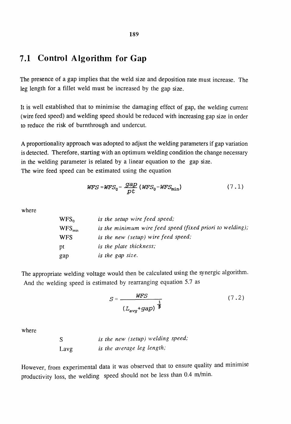
189
7.1 Control Algorithm for Gap
The presence of a gap implies that the weld size and deposition rate must increase. The
leg length for a fillet weld must be increased by the gap size.
It is well established that to minimise the damaging effect of gap, the welding current
(wire feed speed) and welding speed should be reduced with increasing gap size in order
to reduce the risk of burnthrough and undercut.
A proportionality approach was adopted to adjust the welding parameters if gap variation
is detected. Therefore, starting with an optim urn welding condition the change necessary
in the welding parameter is related by a linear equation to the gap SIze.
The wire feed speed can be estimated using the equation
WFS =WFSo- gap (WFS -WFS . ) pt 0 In.l.n
(7 .1)
where
is the setup wire feed speed; WFSo
WFSmin
WFS
pt
is the minimum wire feed speed (fixed priori to welding);
is the new (setup) wire feed speed;
is the plate thickness;
gap is the gap size.
The appropriate welding voltage would then be calculated using the synergic algorithm.
And the welding speed is estimated by rearranging equation 5.7 as
WFS S=------
1 (7 .2)
(Lavg
+ gap) "J
where S is the new (setup) welding speed;
Lavg is the average leg length;
However, from experimental data it was observed that to ensure quality and minimise
productivity loss, the welding speed should not be less than 0.4 m/min.

190
Therefore, if predicted welding speed is less than O.4m/min then the welding speed
should be fixed at ~Am/min and the wire feed speed re-estimated using
1
WFS = S (Lavg + gap) "J
7.2 Control Algorithm for Standoff Variation
(7 .3)
If standoff changes, it can either be corrected through the welding robot program or by
maintaining the welding current at a reference value by controlling the wire feed speed.
This can be done by reversing equation 5.18, that is,
where
SO· I
(7 .4)
is the reference welding current estimated from procedure
using equation 5.18;
is the standoff at interval i.
It was assumed that this would keep penetration relatively consistent inspite of standoff
variation. However, increasing wire feed speed to compensate for reduction in current
will lead to an increase in bead size unless speed is increased to take bead size into
consideration.
The welding speed control equation is
(7 .5)
The appropriate welding voltage would then be calculated using the synergic algorithm.
If any control action is taken, then the constant in the standoff estimation model must
be recalculated using the new wire feed speed and standoff as the reference input values.

191
.--------------,1 computcr-d ______ ---,
I--_W_~,I Controller ideal procedure optiInisation QP ~ algorithm
• -t synergic control
algorithnl
.. control
WP
-- WELDING PROCESS
SENSORS
TP
actual ~--I"~ QP
QP cstim atcd .---_---l.t ____ --. •
.... ,.. control algoritllIl1 I .12P reporting a1gorithm ~ .
+ off-linc quality control systcnl
-monitoring algorithm
QP Quality parameters WP Welding parameters DP Disturbance parameters TP Transient parameters
Figure 7.1: Adaptive Quality Control Concept Algorithm Architecture

Chapter 8
Process Modelling and Procedure
Generation using Artificial Neural Networks
Modelling was an integral part of this work; as a feasibility study of alternative
approach, some of the regression models were remodelled using artificial neural network.
It should be noted that this is not an indepth analysis of modelling using neural network
but an investigation to see if any improvement can be made on the regression models
and identify the scope for its usage.
Backpropagation neural networks were used to develop models that will estimate weld
quality parameters and assess the risk of defects such as inadequate penetration and
undercut at the procedural stage. However, unlike regression models which can be
inverted for procedure development, backpropgation network is not invertible, so the
inverse model of the process has to be learned.
8.1 Modelling Strategy for Backpropagation ANN
The main task in neural modelling is to define the network configuration. This involves
specifying the number of hidden layers, neurons per layer and the network parameters.
The network parameters are the gain, momentum and maximum output error.
In section 2.7.3 some automatic selection of parameters have been suggested and these
were found useful. The most important contribution being the assertion that, to avoid
overfitting and overtraining, the number of weights must be less than the total number
of input parameters!7!. This provides a way of constraining the network size to the
available experimental data. It was decided to start with the one hidden layer with
number of neurons equal to the input layer. The number of hidden layers and neurons
can be increased but subject to this constraint.

193
Another main concern is when to stop training a network, the common approach is to
train a network, to a specified small error. However, the backpropagation algorithm is
similar in some ways to the least square method. Therefore, the network can be
assessed from a statistical perspective of curve fitting.
It was assumed, as in regression analysis, that the total sum of squares of the actual
output data must be equal to or less than the sums of squares of fitted values by
Artificial Neural Networks. It was assumed that the condition for over fitting and
learning is when the coefficient of determination(R2) is greater than one (see Section
2.7.2)
The network training is done in stages and its prediction performance assessed. In the
commercial artificial neural network (NT 5000™) software used, the maximum output
error must be specified. The starting point was fixed at 0.2 (200/0).
Preliminary investigation shows that the assumptions made above are valid, the
comparison of neural networks and statistical model output on new data gives
comparatively the same results.
8.2 Synergic Mode Neural Network Models
Tables 8.1 - 8.4 gives details of the neural network models developed. The network for
procedure development was trained with the experimental data that provided penetration
greater than ten percent of the plate thickness and with no apparent defects.

Table 8.1
Network Details
Name
Training Data
Objective
Input
Output
Training Parameters
Topology
Number of Weights
Momentum of Learning
Learning Rate
Transfer Function
Gain
Statistical Characteristics
R2
Number of Iteration
Validation Result
194
Neural Network Modelling of Leg Length and Throat
Thickness: Synergic Mode
DIPA23
Table 5.2
To predict leg length and throat thickness.
Current, Standoff and Welding Speed
Side and Bottom Leg Lengths and Throat
Thickness
3,4,3
31
0.95
0.15
Sigmoid
3
0.8234
334
Table 1 in Appendix G

Table 8.2
Network Details
Name
Training Data
Objective
Input
Output
Training Parameters
Topology
Number of Weights
Momentum of Learning
Learning Rate
Transfer Function
Gain
Statistical Characteristics
R2
Number of Iteration
Validation Result
Note:
195
Neural Network Modelling of Inadequate Penetration and
Undercut Risk: Synergic Mode
DIPA13
Table 5.1
To predict risk of inadequate penetration and
presence of undercut.
Current, Standoff and Welding Speed
Pr(Sp), Pr(Bp), Pr(und)
3,3,3
24
0.95
0.3
Sigmoid
3
0.91057
13339
Table 2 in Appendix G
Pr(Sp), Pr(Bp) and Pr(und) are possibility values for risk of inadequate side and bottom
plate penetration and presence of undercut (see Section 5.2.1).

Table 8.3
Network Details
Name
Training Data
Objective
Input
Output
Training Parameters
Topology
Number of Weights
Momentum of Learning
Learning Rate
Transfer Function
Gain
Statistical Characteristics
R2
Number of Iteration
Validation Result
196
Neural Network Modelling of Penetration: Synergic Mode
DIPA11
Table 5.2
To predict penetration depth.
Current, Standoff and Welding Speed
Side and Bottom Plate Penetration
3,4,2
26
0.9
0.3
Sigmoid
3
0.99816
4962 Table 3 in Appendix G

Table 8.4
Network Details
Name
Training Data
Objective
Input
Output
Trnining Parameters
Topology
Number of Weights
Momentum of Learning
Learning Rate
Transfer Function
Gain
Statistical Characteristics
R2
Number of Iteration
Validation Result
197
Neural Network Procedure Development: Synergic Mode
DIPA24
Table 5.2
To predict welding procedure giving required bead
siz e and the standoff distance.
Side and Bottom Leg Lengths and standoff
Current and Welding Speed
3,6,2
38
0.95
0.15
Sigmoid
3
0.90106
29445
Table 4 in Appendix G

198
Testing the Networks - Synergic Mode
The neural network models are tested on the same data used to test the regression
models for the synergic mode. The network models give a maximum prediction error
of -O.722mm for leg length, -OA04mm for throat thickness, O.568mm for side plate
penetration and -O.552mm for bottom plate penetration (see Figure 8.1). The undercut
model was not very accurate. The possibility model of penetration was satisfactory.
Pr(Sp) also gives high value at low current.
The artificial neural network was used to generate welding conditions for leg length
between 2.5-4mm on 1.6mm plate thickness. The standoff was fixed at 12mm. All
welds produced from the network prediction are of marginal quality with undercut or
traces of undercut present. It can be seen from the quality of weld obtained that while
penetration is adequate, the dimensional accuracy was not satisfactory (see Figure 8.2).
8.3 Manual Mode Neural Network Models
Tables 8.5-8.8 gives details of the neural network models developed. The experimental
data present a problem that was resolved by a novel modelling logic. The problem was
that the experimental contains spatter and undercut response data. It is perceived
possible to specify acceptable risk of defects, in this case spatter and undercut at
procedure stage.

Table 8.5
Network Details
Name
Training Data
Objective
Input
Output
Training Parameters
Topology
Number of Weights
Momentum of Learning
Learning Rate
Transfer Function
Gain
Statistical Characteristics
R2
Number of Iteration
Validation Result
199
Neural Network Modelling of Leg Length and Throat
Thickness: Manual Mode
DIPel
Table 5.4
To predict leg length and throat thickness.
Wire feed speed, Welding voltage, Welding speed
and Standoff
Side and Bottom Leg Length and Throat
Thickness
4,2,3
19
0.95
0.15
Sigmoid
3
0.7514
1428 Table 5 in Appendix G

Table 8.6
Network Details
Name
Training Data
Objective
Input
Output
Training Parameters
Topology
Number of Weights
Momentum of Learning
Learning Rate
Transfer Function
Gain
Statistical Characteristics
R2
Number of Iteration
Validation Result
200
Neural Network Modelling of Penetration: Manual Mode
DIPe3
Table 5.4
To predict penetration depth.
Wire feed speed, Welding voltage, Welding speed
and Standoff
Side and Bottom Plate Penetration
4,6,2 44 0.95 0.15 Sigmoid
3
0.9454 5340 Table 6 in Appendix G

Table 8.7
Network Details
Name
Training Data
Objective
Input
Output
Training Parameters
Topology
Number of Weights
Momentum of Learning
Learning Rate
Transfer Function
Gain
Statistical Characteristics
R2
Number of Iteration
Validation Result
NOTE
201
Neural Network Modelling of Spatter and Undercut Risk:
Manual Mode
DIPC5
Table 5.4
To assess risk of spatter and undercut from
procedure.
Wire feed speed, Welding voltage, Welding speed
and Standoff
Pr(spatter), Pr(und)
4,6,2
44
0.95
0.15 Sigmoid
3
0.9425
4297 Table 7 in Appendix G
Pr(spatter) and Pr(und) are possibility values for presence of spatter and undercut.

Table 8.8
Network Details
Name
Training Data
Objective
Input
Output
Trnining Parameters
Topology
Number of Weights
Momentum of Learning
Learning Rate
Transfer Function
Gain
Statistical Characteristics
R2
Number of Iteration
Validation Result
202
Neural Network Procedure Development: Manual Mode
DIPC6
Table 5.4
To predict welding procedure giving required bead
siz e, S tando!! and A cceptable de! ect risks.
Side and Bottom Leg Lengths, Standoff,
Pr(spatter), Pr(und), Standoff,
Wire feed speed, Voltage and Welding speed
5,7,3
66
0.95
0.15
Sigmoid
3
0.8568
1369 Table 8 in Appendix G

203
Testing the Networks - Manual Mode
Using the same three weld runs for testing the manual mode regression models on the
neural networks; the maximum prediction error for throat thickness was -0.682mm, for
leg length was -0.914mm, for bottom plate penetration was 0.267mm and for side plate
penetration was 0.436. The response data for undercut model suggest that Pr(und)
greater than 0.20 corresponds to presence of undercut. The response data for spatter does not show a clear cut cluster.
The welding conditions that were generated by the neural network for leg length
between 2.5-6mm on both 1.6 and 3.2mm plate thickness gave very satisfactory welds.
The penetration was adequate and the dimensional accuracy was satisfactory (see Figure 8.3).
8.4 Comparison between Regression Models and ANN
Models in welding are generally used for estimating weld quality from the setup parameters. Comparisons were made between the regression models and neural networks prediction. Initial comparison of the test data suggest that neural networks
produces better models for penetration while regression models produces better models
for the leg length and throat thickness.
However the data was not representative of the process range; the predicted data from
procedure optimisation routine was used as the comparison data (Tables 1 and 2 in
Appendix F) as they are the most representative data available for a wide range of bead
size and welding parameters.
From the results, it can be deduced that neural networks offers no significant
improvement over regression models (see Figures 8.4-8.6); comparative results were
obtained and neither of the modelling methods gave satisfactory prediction for
penetration. An objective comparison of risk of inadequate penetration, spatter and
undercut models was difficult, as their performance is dependent on the level of decision
threshold set. Figure 8.7 shows the correlation between neural networks and regression
models used for prediction possibility of undercut.
The neural network developed for procedure development in the sy nergic mode was not
very satisfactory. However, in the manual mode model, good welding conditions were
generated. The main drawback is that neural network approach only gives one solution
which might not be satisfactory; while statistical approach gives a series of conditions
satisfying the quality objectives to select from. Figures 8.8 and 8.9 shows pictures of
the welds produced by both approaches.

(a) Leg length Actual
Sri ----------------------------------------~
4, .... · ..
3~ ....... :::::+.······ ~~ ;~;J~~~>-. . . . ~...--.-:.-:. . . . ..............
2
1 >-- •..•.•.••••••••••••••••••••••••••••••••.•••••••
• 01 : T • . ;: . .,.. . •
-1 ! • f • If' f J« • I «f 1 •• « I ••• I , • fl. I •• , J ••• I
2 2.2 2.4 2.6 2.8 3 3.2 3.4 3.6 3.8 4
Predicted
Actual (b) Throat thickness
3~r-------------------------~
2.5~ .... ... . 2 f. . . + + . . . . . . . . . . . -----. . . ++ ---.\----- . .......... ----~~+ ~ + + .....
'----~ '" . '" . " .
1.5
1 r- ............................................ .
0.5r-······ .... ~ ................................. .
of P I. ." , . .. 0.5 1
•••••••,·., •••• , •••• , •• , •• ,.!I., .. ""(""""" .. , .. 1 tl .. I I
1.5 1.65 1.8 1.95 2.1 2.25 2.4 2.55 2.7
Predicted
·2.U4
Actual Penetration (c) Bottom plate penetration. 1.5,. --------------
1
, + 0.5t·· "1' ......... . + .... . ..................... -t
~
+ + I~ ok , ! ,." T Nominal Deviation
.4. •
-0.51- ..................................... .
-1 L... ••••••••••••••••••••••••••••••••••••••••••••••
-1.5' .. " ..... !. It", .. I ........ ,! ......... I·· ..... • ...... • .... •
o 0.2 0.4 0.6 0.8 1 1.2
Predicted Penetration
Actual Penetration (d) Side plate penetration
2rl --------------------------------~
1.5,························· .................... .
1
0.5
O~ !'P + L • " J ,
i I I
-0.5 . ................. . ..................... j
-1 I.. .,' I. I, ••• t ••• tit" ••• t •• I, t.'" , I, .,. tit ••••• t. I
o 0.2 0.4 0.6 0.8 1 1.2
Predicted Penetration
Figure 8.1 Testing Neural Network Models for Synergic Mode

205
Actual Leg Length 6.---------------------------------------------~
5 .................................................................... .
4 ............................................ .
3
...............................................................................................................................................
1 ..................................................................... .
o~~~~~~~~~~~~~~~~~~~~~~~
2 2.5 3 3.5 4 4.5 5
Desired Leg Length
Figure 8.2 Testing Neural Network Procedure Development: Synergic Mode
Actual Leg Length 8~--------------------------------------------.
7 .................................................................... >,,,,~
6 . . . . . . . . . . . . . . . . . . . . . . . . . . . . . . . . . . . . . . . . . . . .. ... >.-~//:.:./ . 5 ...................................... _:,;,;*"':': ........................ .
-------------- * 4
~~ ....... ,..- ..... - .......... . ....................... , .. , .. :.:.~' ............................... .
3 ........... . ..fo«~':-~'~':" .... ... ~ ......................................... . /~*
2 ~"<".":':~ ....... ' ........................................................ .
1 .................................................... . .. .. .. .. .. . .. .. .. .. .. .. .. . .. .. .. .. .. .. .. .. .. .. .. .. .. .. .. .. .. . . . .. .. .. .. .. . .. ..
O~~~~~~~~~~~~~~~~~~~~~7
2 2.5 3 3.5 4 4.5 5 5.5 6 6.5
Desired Leg Length
Figure 8.3 Testing Neural Network Procedure Development: Manual Mode

206
(a) Synergic mode
-- ,.
4 .' f--. . . . . . . . . . . . . . . . . . . .... *- . . . . . . . . . . . . . .;/~. . . . . . . . . . . . . . . . . . . . . . . ....
r- * ~ ,./'/ + + +~ .// T ,/ ,....,. 3 5 _ .... *- ................. ~, '.'/*-: ....................................... .
. - 7' ~ ,.../
/' ,,' ,.'
3 _. i· ....... ,;//~--:~'~ . . . . . . . . . . . . . . . . . . . . . . . . . . . . . . . . . . . . . . ............ . - ".,.,,/
," ,'-- /'
,/
t- ,/'// 2.5 ,/ I t I I I I I I
2.5 2.7 2.9 3.1 3.3 3.5 3.7 3.9 4.1 4.3 4.5 4.7 4.9
Actual
(b) Manual mode
Predicted 8~----------------------------------~
f--7 ~ .................................................... * .. *,' '1' . ','/',.~.,>~i
_ ; i- I *,/' 6- ............................................... *- ..... T ,.' . . ~ ~ ., .. - .,.: . . . . . . . . . .
+ REGRESSION * ANN I I I I
1 1.5 2 2.5 3 3.5 4 4.5 5 5.5 6 6.5 7
Actual
Figure 8.4 Comparison between Statistical and Neural Network Models:
Leg Length

207
(a) Synergic mode
Predicted
1r---------------------------------~/~ /'
//
////
I- //
0.8 1-- ....... ---. -. --................... + ................... >"'A./:-':/~' . ........ . f- ;< ~ 'IlL' :,v. /////
f- T ~ ~ ,/
0.6 1-- ..••.•..•.•• + ..... ~ ........... --...... ;.,.~-:/<t ............... + ..... . I- /
)fE//"'
// + * 0.41--" .. '," ... , .............. :.-/-".' ...... + .................................. .
f-';';;' ___ ,./'
,/
f- /'
0.2 1-- ...•.•.... ',.>//-:.--.': .................. - .................................. . I- "..;-/./
/'
~ .,,/"-/ // + REGRESSION * ANN o // I I I I I
o 0.1 0.2 0.3 0.4 0.5 0.6 0.7 O.B 0.9 1
Actual
(b) Manual mode
Predicted 3.5rf------------,-------------------.----------~
I-
~ + REGRESSION * ANN 31--················· f- L......---______________ ----.l ................ >~
I- // I- / 2 ///~
.5 1-- ..................................................... :."">"':":~~~ ...... .
2 t····························· .+ ........ ',>+.«~ ................ . 1 5 f- /~~(/ X X
. f- . . . . . . . . . . . . . . . . . . . . . . . - . . . . . . ~ ,~.: -- -:< . 7 . . . . . -. . . . . . . . . . . . . . . . . . . .... .,./;"'
I- / 1 f-. - .. - ................ ....L.<~ -..... -t + ~*/+ * .... -......................... . ~. ~*,//' t* +
0.5 -+ ~4t>.,~~ .. + .. ~ ......... *. ·to
_';
-t/ +~ * ;:K
O ~.[~'I~ * . f ,- I I I I 1 I
o 0.2 0.4 0.6 0.8 1 1.2 1.4 1.6 1.8 2 2.2 2.4 2.6 2.8 3
Figure 8.5
Actual
comparison between Statistical and Neural Network Models: Bottom Plate Penetration

l
I-
208
(a) Synergic 'mode
+ REGRESSION * ANN
,./; .. /
1.5 .-00000+ 0 0 0.000000.00000000000000 •• . ....... :>,/</: ..... 0 • 0 • 0 •• 0 ••
t-
+ ,.;-'
+ + + 1 f--. 0 0 • 0 • 0 •• 0 • 0 0 0 •• 0 0 0 0 0 0 • 0 0 0 0 0 • 0 0 ,.~,/', ~~.< . 0 • 0 •••••••••••••••••••••••••••••
: + + /// I /,;" ,/
** ./.,.//* * * * 0.5 ..- 0 0 0 • 0 0 0 ¥ 0 0 0 • :;,,:r'''-: . 0 0 0 0 *0 0 "0 • 0 0 ••• 0 • 0 • 0 • 0 0 ••• 0 0 0 •• 0 0 • 0 0 • 0 0 0 ••• 0 0 0 0 •• 0 0
I I t I I 1
" ,'-
,,//..r /'
",../'"
.,/
t- " O~'/
t-
t-
o 0.2 0.4 0.6 0.8 1 1.2 1.4 1.6 1.8
Actual
(b) Manual mode
2
Predicted
51-~--------r-------------~--------~ + REGRESSION * ANN
4 r- ...................................................... . • •• a __ ••• :/:..~~
3 t-- ............................... .
2 f-- .................................. ,/< .. :":' .. . /"
/" ..
Actual
. ........ ;.,/ .... -: .... ~ .... ~ ...... - ...... -
* +
*" "* I J
2.5 3 3.5 4
Figure 8.6 comparison between Statistical and Neural Network Models: Side Plate Penetration

209
R~ression Models 0.8.----------------~
•
+ + + 0.6 I-- _____________________________________________ + ____ D __ _
• •
0.4 ,..... - - -+ --------------------------------+ ---------------
+ . +
•
+ •
+ O. 2 I-- - D- - - - - - - - - - - - - - - - - - - - - - - - - - - - - - - - - - - - - - - - - - - - - - - - - - - - -
D
•
• O~~~~I~~.~I~~I~~~I~~I~I~~I~~I~~~I~~I
o 0.1 0.2 0.3 0.4 0.5 0.6 0.7 0.8 0.9
Artifi cial Neu ral Networks
1
• off-line
+ on-line
Figure 8.7 Comparison between ANN, on-line and off-line prediction for
undercut

2\0
Figure 8.8 Photograph of Welds produced using Regression Model
Approach

2 \ \
Figure 8 .9 Photograph of Welds Produced using Artificial Neural Network Approach

•
Chapter 9
Discussion
9.1 Introduction
The aim of this project was to develop an adaptive quality control strategy for robotic
gas metal arc welding although the work carried out is also applicable to mechanised
welding systems. The work was motivated by the industrial need for on-line quality
control. The target application area, is the manufacturer of welded steel sheet and
tubular components. Typical production is usually high volume and involves producing
components with multiple welds in different welding positions. Each weld could have
different quality requirements, defined by the customer's need.
It has already been established that the reject rates are not high but the manual quality
control method used to monitor and maintain this is expensive7• Their profitability or
even financial survival therefore depends on producing good quality welds at low cost.
Hence, the need for a quality control sy stem with the ability to correct or identify any
quality variation during welding.
Quality is more effectively achieved by avoiding defects. It is therefore important to
establish procedures for producing the required quality welds and for preventing,
detecting and correcting critical quality problems. The critical defects encountered in thin
sheet welding are identified in section 1.1. The strategy for controlling them presented
in section 3.1. A three point approach was proposed; off-line optimisation (procedural
control), on-line control (adaptive control), and post weld analysis for long term
assessment.
These were used to:
optimise welding procedure;
control bead geometry;
prevent insufficient penetration;
prevent undercut;
detect and control metal transfer;

213
assess welding arc stability;
detect variation in joint geometry;
detect variation in standoff;
provide information on process trends.
9.2 Process Modelling
Welding is a special processq that requires skilled operators to achieve optimum
operation. In modelling the welding process, it is important that the models can be
easily interpreted and understood in terms of the system. The models developed in this
work were aimed at emulating the welders' control actions.
A welder in producing welds of adequate quality would ensure that he has good arc
ignition and a stable arc, before moving the arc at a speed that gives appropriate bead
size and good fusion. The action is in fragmented but interrelated stages, hence models
were developed to reflect this situation. The following welding phenomena were
modelled:
Phenomena Modellinl: Objective
1. arc ignition assess risk of bad ignition;
2. process stability assess stability and transfer;
3. undercut assess risk of undercut;
4. penetration quantify penetration depth;
5. gap detection detect gap and burnthrough;
6. bead size quantify bead size;
7. standoff variation quantify standoff variation.
The complete modelling of the welding process involves the integration of various
models each defining a specific aspect of the process. The models were used to monitor
and control the process. It should be noted that the models required were determined
from the specification of quality features and any physical phenomena that affects
quality.
q As defined in B S57 50: Part 1: 1987.

214
The models are classified as either off-line or on-line depending on the parameters used
in developing them. The off-line models are developed using the welding setup and
quality parameters. While, the on-line models are based on process disturbance, transient response and quality parameters.
It should be noted that the relevant parameters defining weld quality depend on the
welding parameters used. Therefore, the quality control problem in welding was treated
as regression problem. Three basic assumptions were made in order to model the
process, using regression methods:
1. It was assumed that the process input parameters have a proportional relationship
although not necessarily linear over a wide operating range (see section 2.6) with
the output parameters;
2. It was assumed that if the arc is stable, then the features of the welding
waveforms are relatively static. Therefore, the transient features which are
interdependent can be modelled empirically. The ability of new generation of
power sources equipped with setpoint controllers makes this assumption
plausible;
3. It was also assumed that the data used for modelling are representative of all
relevant operating conditions and was sufficient to realistically represent the
normal process behaviour.
The process quality output are further classified as qualitative and quantitative.
Qualitative data are features which cannot be defined numerically; whist quantitative
data can be described numerically. Examples of qualitative parameters are undercut and
spatter, while quantitative parameters include leg length and penetration.
The quantitatIve parameters are modelled using a multiple regression method, while the
qualitative parameters are modelled using a fuzzy regression method. The fuzzy
regression output gives a "possibility measure" of a defect occurring. Undercut and
plate fusion were modelled using fuzzy regression.
The benefits of using regression analysis for the process models developed are:
1. it is a standard procedure and easy to use;
2. good for quick model development;
3. statistical software package widely available;
4. models can be built to reflect process understanding;
5. the models can be easily programmed into controllers.

215
The basic drawback however is that, due to simplicity of regression approach, it can
easily be misused and misunderstood. The main source of difficulty in regression
modelling is in determination of a model's structure. It should be noted that the models
are used mainly for predictive purposes in welding applications. Hence, the models'
structure should only be subject to the constraint that they fit the experimental data used.
Although where possible the structure should incorporate any understanding of the
process physical phenomena. It is also proposed that a specification for regression
analysis be established. The minimum values for the correlation coefficient and
statistical significant (a) level for estimated coefficient in final model, should be
specified.
9.3 Process Monitoring
The ability to monitor the process is very critical to the quality control approach
presented here. It should be noted that, "what can't be detected can't be controlled".
The basic objective of monitoring was to provide control signals and report
abnormalities.
From the published work surveyed (section 2.3 and 2.4), it was concluded that defect
diagnosis and quality control for an arc welding process could be achieved by
monitoring the arc electrical characteristics. This implies the need to acquire reliable
data and develop the necessary sensing strategy (including data processing algorithms).
The advent of computers made this task easier, giving the scope for innovative data . d 11· d d· . 219,222 processIng, process mo e lng an lagnosls .
The sensitivity of the arc to disturbances is one of the main requirements for process
monitoring. Process disturbances are reflected as changes in the arc transient and/or
steady state (average) characteristics. The transient features used to detect, monitor or
estimate some process phenomena are shown below:
Phenomena Relevant Features
1. bead profile mean current and voltage;
2. arc stability minimum and maximum current;
3. metal transfer mode background voltage, minimum and maximum
current;
4. penetration mean current and voltage;

5. undercut
6. standoff
7. gap sensIng
8. burnthrough
216
mean current and voltage;
mean current and voltage;
background current and voltage;
background current and voltage
The fault detection methods outlined in section 2.3.4, were used in hybrid form in this
work. The most commonly used techniques are model-based diagnosis and pattern
recognition. The models are developed using regression analysis. Sections 5.4 and 5.5
illustrate the models used for monitoring. The models developed utilises the novel
windowing technique developed by Chawla219• The technique involves the use of a data
acquisition system to capture data in small blocks (windows) of transient data.
This effectively divides the data into a fixed number of segments representing the whole
weld run. It is therefore possible to treat each segment as independent. This also means
that the on-line models can provide output prediction at regular intervals based on each
window data.
However, care is needed in using regression models for monitoring. Regression analysis
is normally based on the assumption that predictor variables in a model are fixed. The
on-line parameters are normally corrupted with randomness due to the process physical
phenomena. The degree of randomness depends on the overall process stability. It
should be noted therefore that the models for predicting bead geometry, penetration and
risk of undercut (section 5.5) are only valid if the arc is established and reasonably
stable (that is have reached equilibrium).
Scope for Statistical Process Control
The main scope for statistical process control would be for post weld analysis. This
would involve the development of a quality management and supervision (reporting)
system or network. The traditional statistical process control (SPC) techniques can be
integrated with the models for monitoring (Sections 5.4 and 5.5). The historical output
of the models can be used to detect sy stematic or sudden changes in process
characteristic such as the occurrence of burnthrough or sudden break in arc.
Implementing adaptive control is a sign that something is wrong, hence any control
action initiated can be reported and logged. The SPC charting of the frequency of
control over a long period can be used to develop a predictive maintenance strategy.
For example, adapting the procedure frequently for gap in a joint that is supposed to be

217
a tight fit can be deemed as an indication of wear in bending and cutting tools.
The stability of the welding arc is greatly influenced by the condition of the contact
tip223. Starting with a stable arc, trends in the stability and transfer indexes developed
in this work over a period can be used as indication of possible wear in the contact tip.
9.4 Procedure Optimisation
Although this work shows that, it is possible to monitor and predict defects, it is clear
from an economical point of view that prevention is even better than identification.
Many potential weld defects can be prevented by proper quality control practice. The
first step in quality control is to weld with an optimum procedure. Welding with an
optimum procedure is important as the damaging effect of any quality disturbance should
not then be very drastic giving time to detect and change the procedure as necessary.
Statistical and neural network based optimisation methods have been successfully
evaluated during this work. The statistical approach offers more flexibility, because it
is based on an iterative strategy. It produces a series of welding procedures that satisfy
the required quality criteria, while artificial neural network predict only one procedure,
the quality of which depends on the design of the network and the validity of the
training data.
The statistical based optImIsation technique was an adaptation of multiobjective
optimisation concept introduced by Deringer and Such204• The technique was illustrated
section 6.5, the primary advantage of this approach lies in its modularity, new models
and constraints can be easily added. The main optimisation objective was the
minimisation of the welding arc power subject to satisfying required quality criteria.
An optimisation routine must not only ensure a stable welding arc, it must also ensure
that the weld pool is in dynamic equilibrium. While the objective of the present work
does not involve the study of weld pool behaviour, its indirect influence on the final
weld quality is recognised, based on the detailed analysis presented37
in section 2.1.4.
The decision to optimise the welding procedure by minimising the arc power (subject
to satisfying the quality requirements) is based on the fact that thin sheets are susceptible
to fitup problems l ,2, which means defects such as burnthrough and undercut could occur
frequently if excessive arc power is used. Therefore, it is assumed that, if the lowest

218
arc power possible (subject to satisfying the quality requirements) is used, the resulting
procedure is more tolerant to fitup problem and positional welds.
The implication of minimising arc power however is that, the welding speed predicted
might be low; the benefit of this is that, there is more time to control and detect
disturbances with more certainty. It should be noted however that as speed increases the
process is less tolerant to disturbances. It is presumed that any industrial productivity
requirement can be satisfied easily from the predicted procedures, as the results in
Appendix F shows; however if required a minimum productivity requirement can be
added as constraint into the optimisation routine.
It should be noted the work carried our was intended for implementation on thin sheets
welding applications, therefore there is a limit to the extrapolation of minimum arc
power as the procedure optimisation criteria on thicker plates.
9.5 Process Control
The process control involves the adjustment of the welding procedure in a pre-specified
manner. The objective is to counteract the effect of disturbances while ensuring the
stability of the process and acceptable quality welds are produced in accordance to
quality requirements.
The main control parameters are wire feed speed, voltage, standoff and travel speed.
The changes necessary are obtained by reversing the regression models based on the
assumptions that the model accuracy is satisfactory. The stability of the control loop is
maintained by the synergic control. It should be noted that the control stability would
also depend on the ability of the welding power source to implement fast and smooth
set point changes.
The control emphasis is on bead size only. The penetration models developed were not
robust enough to be used for control. It was therefore assumed that maintaining current
at a set level will keep penetration adequate. This emphasises the need to start welding
with an optimum procedure.
The proposed control strategy illustrated in sections 3 and 7 is "anticipatory in nature";
that is excessive control are avoided as corrective actions are initiated only if there is

219
going to be a violation of quality requirement. The overall control architecture is shown
in figure 7.1.
The modular structure of the strategy means that each individual module can be used
independently. The modules were independently tested satisfactory off line with the
exception of the control algorithm.
The control algorithm presented in section 7 was implemented in an industrial
environment on a VME (Versa Modular Eurocard) bus system224-225. The communication
between the VME system and the welding system (robot and power source) was done
via a Robot Interface built by Migatronic.
The transfer of welding parameter before and during welding to the power source was
successful; but it was not possible to change robot speed and position during welding.
Hence, the control strategy presented was not fully validated in a closed loop situation.
The software implementation of the control algorithm however shows that with reference
to the quality of welds already obtained, the control routine would maintain good weld
quality and a stable arc.
9.6 Analysis of Investigation
The work done is mainly empirically based. It was based on the premise that there is
a sufficient amount of experimental data representative of the process operating
conditions to develop all the necessary models. It is however difficult to validate this.
The regression models were developed with data from experimental trials. The aim of
the experimental design was to obtain representative data. The most common
experimental approach being used in welding is factorial design; but the result of
parameter selection in this work shows it is not always feasible to use factorial design.
The combinations of some parameters do not produce good fusion welds. It was found
necessary to adjust parameters to get good welds hence restricting the welding parameter
range.
Factorial experimental design was used for trials conducted using the synergic mode of
the power source (section 5.2.1). However, it was found difficult to apply factorial
design in manual mode (section 5.2.2), due to the difficulty in the selection of voltage.

220
This led to the use of "unplanned" experiment for welding with the power source in
manual mode. It can be argued that, this could lead to unrepresentative and biased data.
However, the prediction error of the models developed were acceptable. The importance
of systematic approach to experimental design must however be stressed.
The main problem encountered (which could result in modelling errors) IS bead
asymmetry, that is, unequal leg length. This was attributed mainly to robot
programming problems. Welding in horizontal vertical position is likely to make
tendency towards bead asymmetry increase with current. To reduce the misalignment
effect on modelling, the leg length would be expressed in this project as the average of
both leg lengths. The bead asymmetry range observed in the experimental study is
shown in Table 1 in Appendix H.
The independent parameter range can also affect the ability to produce representative
models. The independent parameters for synergic mode were found to be too limited.
The range of variables which may be used produce no defects apart from the fusion
problem encountered, may be due to the speed range used (0.8-1.6m/min), although the
models were tested for speed as low as O.4m/min and satisfactory results were obtained
as is shown in Appendix A. This gives an indication of the effectiveness of the synergic
control algorithm used.
The problem identified was rectified in experimental trials for manual mode, the speed
was set between 0.3-1.6m/min. Tables 2 and 3 in Appendix H gives the welding and
bead response parameter range respectively. However, investigating a wide range of
parameters leads to some difficulty as voltage is not easily controllable. This however
in the author's opinion is not a setback, since experimental studies are supposed to
represent the process behaviour. The use of synergic welding has the benefit of
automatic control of critical parameter such as voltage, but at the expense of establishing
potential defect patterns and parameter tolerance.
Evaluation of the Models
Due to the fact that the models are integrated, it was found necessary to evaluate each
model individually. The models developed for bead size, undercut, gap detection,
spatter generation and arc ignition are found to offer good performance. The penetration
model accuracy was not good but gives satisfactory results in terms of expressing the
posssibility that penetration is adequate or inadequate. That is, using "if-then" (rule
based) approach.

221
The difficulty in modelling penetration can be attributed to the experimental response
level and complexity of the phenomena. The penetration depth is very limited often less
than Imm hence not giving the scope for good generalisation. The industrial
requirement for penetration is very specific; it is either adequate or inadequate; which
suggests the need for fuzzy regression approach for different plate thickness.
Most manufacturing companies do not however have the time for extensi ve modelling
work. In the automotive industry the design thickness of plate may vary from 1 to
6mm. In this case intuitive judgment was used to compensate for the absence of the
desired model precision and adaption of penetration models to different plate thickness.
It was assumed that the penetration models would be valid for plate thickness up to
6mm. Although, the models were not accurate, satisfactory results were achieved when
the manual and synergic models were transferred to 1.6 mm (thinner) and 3.2mm
(thicker) plates respectively.
Main concern was the attainment of adequate fusion on thicker plates and prevention of
overpenetration or burnthrough on thinner plate. The risk of fusion problem is greater
with dip transfer welding of thicker plates. It should be noted that the heat from the arc
is used to melt the plate and as plate thickness increases the energy required to achieve
melting also increases. Middleton226 states that the volume of parent plate melted is
dependent on the arcing current; the arcing current has direct correlation with voltage
and wire feed speed. This is in line with the observation made in section 6.2, that a
minimum voltage exists for a given plate thickness especially in dip welding with the
welding speed set accordingly for the required weld size subject to having a stable arc.
Evaluation of the Algorithm
The models developed were used to design algorithms for synergic control (section
5.3.5), gap detection (section 5.4.2), standoff estimation (section 5.4.1), process stability
assessment (section 5.3.2), procedure optimisation (section 6) and quality control (section
7).
The algorithms all give satisfactory results and have been validated in the laboratory and
tested in an industrial environment where the component welded was a car rear axle.
Appendix I shows an example of the test results; the overall accuracy of welds obtained
was satisfactory, although some of the welds showed bead asymmetry associated with
positioning problems; which can be corrected.

222
The results show that the models can be transferred to other power sources. The
validation in the industrial environment was carried out on a different power source
Migatronic BDH 550; during monitoring the predicted geometry was recorded and
compared with actual welds, the overall accuracy of the welds obtained was satisfactory.
The monitoring rules (see Table 5.7 and Figure 5.11) were also tested on a Murex
TransMIG 450i power source with different gas mixtures; good results were obtained(see Appendix C).
The gap detection algorithm requires more study so as to develop a more precise
modelling approach. The parameters in the algorithm were "fine tuned" to produce a
good fit with simulated gap conditions. The procedure optimisation algorithm developed
was adapted successfully to weld joints with fit-up problems and/or in position by
limiting the operating range of the process to dip transfer. This however depends on the
ability to constrain the metal transfer by integrating the optimisation algorithm with the
synergic control algorithm developed.
9.7 Modelling using Artificial Neural Networks
It has to be noted that there has always been debate between statisticians and neural
networks researchers on the effectiveness of both approaches for emperical modelling,
judgement however depends on personal bias as can be seen in the published work by
Sarle227 and several po stings on comp.ai.neural-nets newsgroup on the Internet. The
objective of the present comparison in this work is not to contribute to this debate but
as exploration of alternative modelling tools for the welding process.
d 11' . Id' 182-188 Regression models have been commonly used for process mo e lng In we lng ;
however artificial neural networks are now being used to solve problems that have been
satisfactorily modelled using regression methods. The limitation associated with the
regression models include the difficulty in capturing the complexity and non-linearity
of the welding process.
The main advantage of regression models over neural network is that they can reflect
physical understanding of the process while the inner workings of neural networks are
difficult to understand and are viewed as a black box. However, the significant
advantage of neural network techniques over regression models is that they offer a non
linear and multi-dimensional (parallel) modelling process with high processing speed.

223
Modelling work using neural networks have been undertaken widely196-198 but none of
the investigators have compared their results with alternative regression models. This
comparison was made in this work. It was concluded from the comparison between
some of the regression models, that the neural network approach offered no significant
improvement over regression models. The accuracy of neural network is comparable
with the accuracy achieved by regression models (see Figures 8.4-8.6) when the
objective was to predict weld quality from a given welding procedure.
However, using backpropagation neural network models for procedure development
requires practical welding experience. A real process representative input-output
response (experimental) data is fundamental to good model performance. The poor
performance of the sy nergic mode neural network for procedure development shown in
figure 8.2 illustrates this. The procedure development neural network for the manual
mode shows that the network must be trained on data containing information on
potential defects and problems.
The results of the work carried out shows that both techniques satisfactorily model the
welding process and can therefore be used to complement one another. Although this
is not an extensive study, it was identified that neural networks can be integrated into
the strategy developed. Neural networks can be used to replace the fuzzy regression
models because they produce output between 0 and 1 without the need for the
constraints employed on the fuzzy regression models output. They can also be used for
process monitoring and diagnosis.
For example the stability rules in Table 5.7, are very subjective and involve knowing
how the process behaves to establish the thresholds. A neural network was used to
reduce the complexity of the IF .. THEN rules. The neural network can be used to
classify transfer mode and assess stability by using the transfer, transfer stability and dip
consistency indexes as input into the network.
To do this, it was assumed that metal transfer consist of both dip and spray components.
The spray component (Pr(spray)) represent the tendency for a droplet to transfer without
short circuiting and dip component (Pr(dip)) vice-versa. The amount of each component
present depends on how unstable the process is. The actual transfer mode and stability
depends on the dominant component.
The use of a threshold is unavoidable but its complexity can be reduced using the ANN
approach. The applicable thresholds would have upper and lower value within which

224
the process would be considered unstable. Section 2.3.5 discussed the issues involved
in threshold selection. The network tested in this work was trained on data used for
validating the synergic algorithm (Table 5.10). The data was coded as follows:
if dip transfer Pr(dip)=l and Pr(spray)=O
if spray transfer Pr(dip)=O and Pr(spray)=l
The trained neural network details are shown in Table 9.1
Table 9.1 Neural Network Modelling of Metal Transfer Mode Detection
Topology 3,3,2
Number of connections 20
Input TI, TSI, DCI
Output Pr(dip), Pr(spray)
Momentum 0.95
Learning Rate 0.15
Gain 3
Iteration Number 158
Output Error 0.004
It should be noted that regression models can also be used. The regression models
developed are:
pr(spray) =O.485+0.655TSI-l.1983DCI-2.601TI (9.1)
Pr ( dip) = 1 - Pr ( spray) ( 9 . 2 )
The regression models however seem very sensitive compared with neural network.
The table in Appendix J shows the response of the neural networks and regression
models to the manual mode experimental data (Table 5.8).

225
9.8 Possible Industrial Applications
As already stated, this work was motivated by the industrial need. The algorithm
developed has been implemented on a VME computer system and tested in an industrial
environment225
• The trials were satisfactory and point to the following possible industrial applications:
1. A daptive control system for weld quality;
The major industrial benefit of this work is the design of a flexible adaptive
control and monitoring sy stem for arc welding processes with the emphasis on
weld qUality.
2. Design of intelligent power sources;
The most significant contribution of the work is probably the monitoring rules
for stability assessment developed (section 5.3). The simplicity of the models
means that they can easily be built into a power source controller. The rules
could be used as basis for the design of an intelligent power source using fuzzy
logic and/or neural networks.
3. Testing and Optimisation of consumable and power sources welding
performance;
It has already been established that the indices in the monitoring rules (section
5.3) seem to be equipment and consumable independent. The indices in the rules
provide a way for testing and optimising the welding performance of power
sources and/or consumable. Dixon220 used the rules for assessing gas mixture
optimisation for robotic welding. The stability models can also be used to give
an objective assessment of inductance and slope requirement for shielding gases
as the results of independent experiment performed by Bassett and Norrish in
Appendix C suggest.

226
4, Development of software tools for welding,
Most modelling work in welding results in application based software, ranging
from monitoring software, numerical and expert system based procedure optI'mI'satI'on softwa 179.180.182.184.219 F 11' h re . 0 oWIng t e same route, a BASIC
demonstration software package was written. The software demonstrates how the
models and algorithm developed were used for quality assessment, defect
prediction, procedure optimisation and enables the simulation of welding
parameter generation and defect prediction. The demo disk is available with the
thesis and the instruction for use are presented in Appendix K.
9.9 Limitations and Possible Improvement for Industrial
Application
Some of the limitations identified are based on discussion with a welding equipment
manufacturer in Europe, in an attempt to establish whether the work could be exploited
industrially.
The quality control strategy presented is empirically based and requIres some
commitment to experimentation. The first concern was that the design of experiment
and building the models might be too time consuming. There is also a problem of
establishing model structure; and ensuring that the experimental data available is
adequate. These concerns can be resolved by automating the design of experiment and
model building technique. This has the added benefit of ensuring consistency and
reliability of the concept presented.
The models have fixed coefficients and are restricted to specific conditions, such as gas,
wire and joint types. For different conditions trials have to be carried out and new
coefficients calculated. The coefficients are normally stored in the equipment in board
memory. The second concern was that the maintenance of different coefficients and
thresholds involved in the models for a wide range of different gases, wire type and
sizes could lead to memory problem. To resolve this concern, practical judgement could
reduce the experiment trials significantly. The models can be developed; however, for
standard joints, gases and wire diameters and programmed into the power sources. The
most important part of the model requirement being to set stable voltage for the wire
feed level.

227
If a new condition is demanded, the programmed condition closest to the new situation
should be selected. The arc could be made stable by increasing or decreasing voltage
as necessary, to ensure stability. It should be noted that most power sources already
have voltage trim facility for doing this. The monitoring rules in section 5.3 and fuzzy
logic (and/or neural network) can be used here to make the fine tuning systematic. An
example of such application can be seen in the published work by Won and Chol44. The
authors used fuzzy logic and rule based method to establish stable arcs for dip welding
trials.
The third concern was how fast the welding signal must be sampled and model output
calculated for closed loop control. It has to be stated that the concept does not require
high sample rate. In setting sampling rate, sampling theorem suggests that signals
should be sampled at twice the rate of the highest signal frequency that needs to be
monitored. Consideration must be given to the sample size also referred to as window.
A window in the Arcwatch ™ contain 512 data points as default but can be set to 256,
1 024 and 2048 data points.
It was assumed that a window must contain approximately 1 0 process cycles. A cycle
is the time taking to transfer a droplet; typical cycle time obtained for a series of stable
welding conditions, using the developed synergic algorithm was between 2 and
16milliseconds (see Table 5.10). The sample rate (per channel) should be set to achieve
this. It was found adequate to set the sample rate in kHz, at the number of data points
per window divided by ten times the cycle time in milliseconds. For the default sample
size of 512 data points, the sampling rate would therefore be between 3 and 25kHz and
the approximate sampling time will be between 25 and 128milliseconds.
The model output would only be constrained by the speed of the computer being used.
On a 33MHz DX2 personal computer it took approximately 1second to implement the
procedure optimisation routine. It is estimated that it will takes approximately
3milliseconds to calculate the welding waveform statistical features for a window
(sample); the features are then used as inputs in to the on-line models and monitoring
rules hence no processing overhead perceived. It is therefore estimated that the control
cycle illustrated in Table 7.1 will take roughly 3milliseconds.
It should be noted that with the techniques used here there is an inherent control delay
time corresponding to the sampling time. The control frequency depends on the rate at
which the welding equipment (power source and robot) can recieve control intructions
(error signals) and update the welding procedure; typical rates of control reported in

228
published work is of the order 5Hz. The sampling times are generally set to
accommodate this and are found to be up to 500milliseconds112• However the control
system can be designed to have different update rate for process control and monitoring.
It is perceived from the result of the current work that reliable high monitoring and
reporting update rate of between 7 to 40Hz is achievable with the sy stem providing on
line graphical display of the models output for the operator(s).

229
Chapter 10
Conclusions and Recommendation for
Further Work
10.1 Conclusions
1. The welding process can be effectively modelled by breaking down the process into well defined sequence of sub-objectives; and integrating the resulting
models;
2. A robust optimisation technique using statistical models and rules derived from weld quality specifications was developed;
3. It was found sufficient to monitor weld quality using welding current and voltage transient signals only and travel speed;
4. The control strategy shows the feasibility of using regression models for adaptive
control of weld quality;
5. A general quality control algorithm architecture has been successfully developed
for gas metal arc welding process;
6. A novel method has been developed for metal transfer detection and process
stability assessment;
7. A thru-arc sensing strategy has been developed for monitoring and estimating the
size of joint geometrical variation (gap):
8. A novel synergic and metal transfer algorithm that combines the transient and
steady state dynamic of the welding arc was developed;
9. Backpropagation neural network models were found to offer no significant
improvement over regression models;
10. The possibility of using backpropagation neural network to reduce complexity
of monitoring rules for some parameters was identified.

230
10.2 Recommendation for Further Work
This project has demonstrated the possibility of developing a flexible quality focused
adaptive control strategy for robotic welding of thin steel sheet. The following further
work is suggested to enhance the usefulness of the results:
1. Development of Knowledge based Experimental Design System
It is important for any experimental design to produce process representative data. The
result of this study has illustrated the difficulty in applying standard experimental design
to welding over a relatively wide range. Hence, a knowledge based system for
experimental design in welding could be developed. The guiding aim should be to
collect data representative of all possible process characteristics.
Welding is a special process, which depends on the skill of the operator. Therefore in
designing an experiment it is important to use the welder's skill. The system should
interact with the welder(s) and be designed to get maximum welder experience by
recording experimental observations. An extension of such a system could include
automating data collecting, analysis, correlation, transformation of observations and
process modelling.
The typical experimental design is envisaged to be evolutionary, taking into
consideration welders' skill and experience. An expert systems could be used to advise
on the next experimental point or whether to continue, based on the response of interest
which must be defined by the quality specification.
2. Extension of Experimental Scope and Range
The experimental work done and models developed could be extended to thicker wire
(say up to 2mm), flux-cored wires, different shielding gases, thicker plate thicknesses
(upto 12mm), other joint geometry, and mUlti-pass welds. The possibility of integrating
the synergic algorithm developed with a pulse synergic algorithm could also be
investigated.

231
3. Process Modelling and Control using Spreadsheet
Commercial spreadsheet software is becoming very powerful with built-in analytical and
statistical function libraries together with powerful charting facilities. Some neural
network software is now being provided as an "add-in" for standard spreadsheets.
A standard spreadsheet package such as Excel and Lotus could be used to develop a
software environment for interactive procedure generation and assessment environment
based on models developed using neural networks and/or statistical methods.
The final system could allow the user to asses the impact of changing welding
parameters by generating alarms for out of specification conditions and offering
corrective advice. The scope for automatic on-line weld quality control and
documentation should be explored.

References
1. Cowan, K. When to integrate welding and vision with robots. Automation, November 1991, pp 68-72.
2. Agapakis, J. and Katz, J. An approach for knowledge-based sensor-controlled robotic welding. Recent Trends in Welding Science and Technology, Proceedings 2nd International Conference, 14-18 May 1989, Gatlinburg , TN.
3. British Standard Quality Vocabulary BS 4778 Part 1, 1987.
4. Norrish, J. Advanced welding processes. lOP Publishing, Ltd, 1992.
5. Phillips, A. Statistical control of weld qUality. AWS Welding Handbook Fundamentals of Welding, 6th Edition, 1968.
6. Volchenko, V. Possibilities of statistical control of the quality of welded joints. Welding Production, 18(4), 1971, pp 1-6.
7. Brite-Euram Project BE-4006-90, Process Control for Flexible Joining System: Technical Report Sub-Task 1.4: Statistical Analysis of Weld Defects.
8. Cornu, J. Advanced welding systems, Vol. 2. Consumable electrode processes. IFS and Springer-Verlag, 1988.
9. Metals Handbook 9th Edition vol. 6, Welding, Brazing and Soldering, ASM.
10. Norrish, J. and Richardson, I. Metal transfer mechanisms. Welding and Metal Fabrication, Jan/Feb pp 17-22.
11. Pokhodnya, I. A method of investigating the process of melting and transfer of electrode metal during welding. Automatic Welding, No.2, 1964, pp 1-7.
12. Lebedev, A. Examination of controlled transfer of electrode metal in CO 2 welding. Paton Welding Journal, 3(3), pp 198-202.
13. Mathews, D. GMA W, short circuiting mode: Stabilities, instabilities and joule heating
model. Vanderbilt University, TN, MSc Thesis, 1988.
14. Classification of metal transfer on arc electric welding processes. Welding in the World,
15(5/6), 1977, pp 113-117.
15. Ushio, M. et al. Effects of shielding gas composition on metal transfer phenomena in high current GMA welding. Trans JWRI, 20(1), 1993, pp 7-12.
16. Sicard, P. and Levine, M. An approach to an expert robot welding system. IEEE Trans on Systems, Man and Cybernetics, 18(2), 1988, pp 204-222.

233
17. Lucas, W. Choosing a shielding gas-Part 2. Welding and Metal Fabrication 60(6) 1992 pp 269-276. ' , ,
18. Stenbacka, N. and Persson, K. Shielding gases for gas metal arc welding. Welding Journal, 68(11), 1989, pp 41-47.
19. Lyttle, K. and Stapon, W. Select the best shielding gas blend for the application. Welding Journal, November 1990, pp 21-27.
20. A guide to shielding gases for gas metal arc welding. Welding Quarterly, September 1988, pp 12-15.
21. Wyant, A. et al. An investigation of methods for evaluating welding arc stability and their application. Welding Journal, Vol. 27, 1948, pp 502-s-514-s.
22. Philpott, M. Direct arc sensing for robot MIG welding. Cranfield Institute of Technology, PhD Thesis, 1986.
23. Xie, X. Weld quality disturbance and its prediction in GMA W. Lund University, Msc Thesis, 1989.
24. Gupta, S. et al. Application of statistical analysis for process stability evaluation in GMA welding. IIW-Doc. 212.710-88, 1988.
25. Dyurgerov, N. Reducing metal spatter and stabilising the process of welding with a short arc. Automatic Welding, No.6, 1972 pp 36-37.
26. Dubovetskii, S. The application of statistical models of weld formation to the design and control of automatic welding conditions. Welding Institute Conference: Advanced Welding Systems, November 1985.
27. Amin, M. Pulse current parameters for arc stability and controlled metal transfer in welding. Metal Construction, 15(3) 1983, pp 272-278.
28. Mita, T. et al. The estimation of arc stability of CO 2 gas shielded arc welding. Welding Institute Conference: Advanced Welding Systems, November 1985, pp 261-271.
29. Dyurgerov, N. Bridge rupture between electrode and molten pool. Welding Production, No.3, 1972, pp 5-8.
30. Zaruba, 1. and Dymenko, V. Regulation of the parameters of the process of welding with short-circuiting. Automatic Welding, No.8, 1971, pp 44-46.
31. Lebedev, V. and Medvedenko, N. Research into the effects of transient processes on metal spatter in CO2 welding. Automatic Welding, No.5, 1968, pp 12-16.
32. Lebedev, V. On technological (welding) properties of power sources for arc welding. IIW Doc. USSR Academy of Sciences, USSR National Welding Committee, 1979.

234
33. Lipei, 1. et al. The effect of the dynamic behaviour of welding rectifiers on spatter. Welding International, No.3, 1988, pp 263-268.
34. Jennings, C. Dynamic characteristics of DC welding machines. Welding Journal, February 1951, pp 117-138.
35. Scotti, A. Process modelling to establish control algorithm for automated GMA W. Cranfield Institute of Technology, PhD Thesis, 1991.
36. Halmoy, E. The pressure of the arc acting on the weld pool. Proceedings International Conference: Arc Physics and Weld Pool Behaviour. The Welding Institute, London 1979.
37. Paton, B. et al. Certain special features of the formation of welds made at high speeds. Automatic Welding, No.8, 1971, pp 1-6.
38. Larson, L. Metal transfer in the metallic arc. Welding Journal, February 1942, pp 107-s-112-s.
39. Wilkinson, M. Root run formation in mechanised vertical MIG arc welding. Welding Research International, 9(4), 1979, pp 60-103.
40. Spiller, K. The process options and manual techniques for welding of pipework fabrication. Advances in Process Pipe and Tube Welding Techniques, Conventry, 17th May 1984, Seminar Handbook.
41. Tuthill, R. Dip transfer carbon dioxide welding. Welding Journal, October 1959, pp 976-981.
42. Zaruba, I. et al. Effects of the method by which the short-circuit current is limited on the formation of vertical and overltead CO2 welds. Automatic Welding, No.4, 1973, pp 61-64.
43. Istolbov, V. and Masakov, V. The formation of burnthrough in the fusion of welding of thin sheets. Welding Production, No. 10, 1977, pp 26-28.
44. Bolmjso, G. Robotic arc welding - Programming and Control. IFAC Robot Control, Karlsruhe, FGR, 1988, pp 541-564.
45. Kloos, K. and Dilthey, U. Using robotic technological systems for arc welding. Paton Welding Journal, 3(17), 1991, pp 546-550.
46. Budai, P. and Torstensson, T. A power source for advanced welding systems. Welding Institute Conference: Advanced Welding Systems, November 1985, pp 424-433.
47. Kolasa, A. et al. Experimental study on dynamic properties of power sources for MIG/MAG welding. Transactions of JWRI, 14(2), 1985, pp 55-65.

235
48. Amin, M. and Nasser, A. MIG power sources with one knob control. Metal Construction, 18(7), 1986, pp 418-424.
49. Manz, F. Inductance vs slope control for gas metal arc power. Welding Journal, 1969, pp 707-712.
50. Popkov, A. Causes of spatter loss in welding with the short circuiting Co shielded arc. Welding Production, No.5, 1971, pp 20-23. 2
51. Ishchenko, Y. and Dyurgerov, N. The mechanism of periodical short-circuits of the arc gap and the stability of welding with a short arc. Welding Production, No.9, 1963, pp 17-23.
52. King, F. and Hirsch, P. Seam tracking systems with the arc as sensor. Advances in Welding Processes, 4th International Conference, Harrogate, 9-11 May 1978.
53. Kannatey-Asibu, E. Analysis of the GMA W process for microprocessor control of arc length. Trans. AS ME Journal of Engineering for Industry, Vol 109, May 1987, pp 172-176.
54. Ide, E. et al. A control system of wire feed rate for stability of GMA welding process. IIW Doc. XII-1276-92, 1992.
55. Middleton, P. and Nonish, J. Progress in controlled transfer welding. Welding and Metal Fabrication, November 1990, pp 497-503.
56. Middleton, P. Synergic algorithms to relate wire feed rate to arcing current for conventional GMA welding. IIW Doc XII-1165-90, 1990.
57. Amin, M. and Naseer-Ahmed, A. Synergic control in MIG welding - steady DC open arc and short circuiting arc operation. Advances in Joining and Cutting Processes, 30th-2nd November 1989, Harrogate, TWI International Conference pp 61-71.
58. Needham, J. Control in short-circuit MIG arc welding. TWI International Conference on Advanced Welding Systems, 1985, pp 331-339.
59. Popkov, A. et al. Reducing the spatter of liquid metal in CO 2 welding by means of optimisation of the welding parameters. Welding Production, No.3, 1977, pp 26-27.
60. Manz, A. The "One Knob Welder". Welding Journal, September 1968, pp 720-725.
61. Blakeley, P. Who should be using arc monitoring. Welding and Metal Fabrication,
58(5), 1990, pp 268-272.
62. VanDoren, A. Data acquisition systems. Reston publishing Company, Inc., 1982.
63. Lucas, W. Computers in arc welding - the next industrial revolution. Part 3: Instrumentation and process analysis. Metal Construction, 17(7), 1985, pp 431-436.

236
64. Rehfeldt, D. et al. Microcomputer-based instrumentation for analysing and monitoring arc welding processes. TWI 3rd International Conference: Computer Technology in Welding, 1990, pp 36-45.
65. Stein, 1. and Dornnfeld, D. A classification and design methodology for manufacturing process sensor systems. 1990 Japan-USA Symposium on Flexible Automation - A Pacific Rim Conference - ISCIE, Kyoto, Japan, pp 675-679.
66. Wells, A. Jr. Through-the-arc sensing and control methods in robotic arc welding. Vanderbilt University, TN, PhD Thesis, 1988.
67. Hanright, 1. Robotic arc welding under adaptive control - A survey of current technology. Welding Journal, November 1986, pp 19-25.
68. Manz, F. Welding arc sounds. Welding Journal, May 1981, pp 23-27.
69. Arata, Y. et al. Investigation on welding arc sound (Report llI) - Effects of current wavefonns on TIG welding arc sound. Trans of JWRI, 9(2), pp 25-29.
70. Morgan, C. et al. Visual guidance techniques for robot arc welding. Proceedings of the 3rd International Conference on Robot Vision and Sensory Controls, 6-10 November 1983, C(IIl bridge, Massachusetts, USA, pp 615-623.
71. Keijzer, A. and Groot, R. Laser based arc welding sensor monitors weld preparation profile. Sensor Review, January 1984, pp 8-10.
72. Shepherd, P. A contribution to adaptively controlled robotic arc welding. Loughborough University of Technology, PhD Thesis 1985.
73. Kremers, 1. et al. Development of a machine vision based robotic arc welding system. 13th International Symposium on Industrial Robots and Robots 7 Conference Proceedings: Future Directions Vol. 2, 17-21 April, 1983, Chigaco.
74. Nomura, H. et al. Automatic seam tracking and bead height control by arc sensor. "Sensors and Control Systems in Arc Welding", Technical Commission on Welding Processes, Japan Welding Society, 1991, pp II-114-120.
75. Iwaki, S. Application of arc sensor to robotic seam tracking. "Sensors and Control Systems in Arc Welding", Technical Commission on Welding Processes, Japan Welding Society, 1991, pp II-80-84.
76. Fukuola, H. A pplication of torch sensor to arc welding robot. "Sensors and Con~rol Systems in Arc Welding", Technical Commission on Welding Processes, Japan Welding Society, 1991, pp II-129-131.
77. Ors zag h, P. and Seneak., V. Adaptive control of torch position with arc sensor. International Journal for JaM, 2(2), 1990, pp 46-54.

237
78. Wild, W. et al. Investigation of arc sensing equipment for a seam tracker in MIG/MAG welding. Welding International, 5(4), 1991, pp 327-331.
79. VanDoren, A. Data acquisition systems. Reston Publishing, Company, Inc., 1982.
80. Schellhase, M. Investigation into arc welding process monitoring by statistical signal analysis. IIW-Doc. 212-491-81,1981.
81. Love, P. and Simaan, M. Automatic recognition of primitive changes in manufacturing process signals. Pattern Recognition, 21(4), 1988, pp 333-342.
82. Frank, P. Fault diagnosis in dynamic systems using analytical and knowledge-based redundancy - A survey and some new results. Automatica, 26(3), 1990, pp 459-474.
83. Peleg, K. et al. A utomated classification of electrical appliances on a production line. NDT International, 21(6), 1988, pp 438-445.
84. Himme1blau, D. Use of artificial neural networks to monitor faults and for troubleshooting in the process industries. IF AC On-line Fault Detection and SupelVision in the Chemical Process Industries, Delaware, USA, 1992, pp 201-202.
85. Tulpule, S. and Galinaitis, W. Health monitoring system for SSME - Fault detection algorithms. AIAA-90-1988, 1990.
86. Dimitroff, G. Statistical process control: A key element of total quality management AIAA-89-2289, 1989.
87. Pap ritan , J. and Helzer, S. Statistical process control for welding. Welding Journal, 70(3), 1991, pp 44-48.
88. Montgomery, D. Introduction to statistical quality control. John Wiley and Sons, 2nd Edition, 1991.
89. Juran, 1. and Gryna, F. (Editors). Juran's quality control handbook. McGraw Hill, 4th Edition, 1988.
90. Radharamanan, R. et al. Sensitivity analysis of the CUSUM method. Int. Journal of Production Economics, 33(1-3), 1994, pp 89-95.
91. Whiteley, 1. and Davis, 1. Qualitative interpretation of sensor patterns. IEEE Expert, April, 1993, pp 54-63.
92. Gertler, 1. Survey of model-based failure detection and isolation in complex plants. IEEE Control Systems Magazine, December 1988, pp 3-11.
93. Smith, C. and Rider, G. Predicting defects in welds. Welding Institute Conference: Advanced Welding Systems, November 1985, pp 239-25l.
94. Frenzel, L. Understanding expert system. Howard W. Sams and Co., 1st Edition, 1987.

238
95. Ghasemshaki, M. and Middle, 1. An expert system approach to the control of welding procedures. TWI Conf. Automated Welding Systems in Manufacturing, Gateshead, North East, UK, 17-19 November, 1991, Paper 5.
96. Taylor, W. Expert systems to generate arc welding procedures. Metal Construction, 18(7), 1986, pp 426-431.
97. Da Costa, S. The prediction of risk of welding defects at the procedure stage using computer knowledge based system. Cranfield Institute of Technology, PhD Thesis, 1992.
98. Nakajima, 1. et al. Torch sensor abd arc sensor for arc welding robots. "Sensors and Control Systems in Arc Welding", Technical Commission on Welding Processes, Japan Welding Society, 1991, pp 11-74-79.
99. Miller, C. Guidelines to gain self sufficiency in robotic welding. Welding Journal, 68(11), 1988, pp 41-45.
100. Kim, J. and Na, S. A study on an arc sensor for gas metal arc welding of horizontal fillets. Welding Journal, 70(8), 1991, pp 216-s-221-s.
101. Kim, 1. and Na, S. A study on prediction of welding current in gas metal arc welding, Part 2: Experimental modelling of relationship between current and tip-to-workpiece distance and its application to weld seam tracking system. Proc. Instn. Mech. Engr., Vol 205, Part B: Journal of Engineering Manufacture, 1991, pp 64-69.
102. Kim, 1. and Na, S. A study on arc sensor algorithm for weld seam tracking in gas metal arc welding of butt joints. Proc. Insto. Mech. Engr., Vol 205, Part B: Journal of Engineering Manufacture, 1991, pp 247-255.
103. Cook, G. et al. Electrical arc sensing for robot positioning control. International Trends in Manufacturing Technology, Robotic Welding Edited by 1. D. Lane, IFS UK, 1987.
104. Sugitani, Y. et al. Adaptive control of weld bead shape utilizing arc sensor in one side GMA W process with backing plate. IIW Doc. XII-1360-94, 1994.
105. Koves, A. Analysis of welding signals in robotic welding process depending of the gap width. IIW Doc. XII-1227-91, 1991.
106. Davis, A. On-line gap detection techniques for adaptive control of GMA W. Cranfield Institute of Technology, MSc Thesis, 1993.
107. Inoue, K. et al. Measurement of arc sound with bum-through III MAG welding. Welding International, 70(10), 1993, pp 770-775.
108. Johnson, J. et al. Detection of metal transfer mode in GMA W. Recent Trends in Welding Science and Technology, TWR'89: Proc. of the 2nd Int. Conf. Gatlingburg,TN, USA, 14-18 May 1989, pp 377-38l.

239
109. Rhee, S. and Kannatey-Asibu, E. Observation of metal transfer during gas metal arc welding. PED-Vol 51, Welding and Joining Processes ASME.
110. Brandi, S. et al. Analysis of metal transfer in shielded metal arc welding. Welding Journal, October 1991, pp 261-s-269-s.
Ill. Cheryshov, G. and Spitsyn, V. Dynamic action of the arc, burning in CO2
on the weld pool. Welding Production, No.4, 1971, pp 8-9.
112. Lui, S. et al. Metal transfer mode in gas metal arc welding. Recent Trends in Welding Science and Technology, TWR'89: Proc. of the 2nd Int. Conf. Gatlingburg,TN, USA, 14-18 May 1989, pp 475-479.
113. Smartt, H. et al. Sensing and control problems in gas metal welding. Recent Trends in Welding Science and Technology, TWR'89: Proc. of the 2nd Int. Conf. Gatlingburg,TN, USA, 14-18 May 1989, pp 917-921.
114. Clark, D. et al. Drop transfer mechanisms in GMA W. Recent Trends in Welding Science and Technology, TWR'89: Proc. of the 2nd Int. Conf. Gatlinburg,TN, USA, 14-18 May 1989, pp 371-375.
115. Adam, G. and Siewert, T. Sensing of GMAW droplet transfer modes using ERIOOS·l electrode. Welding Journal, March 1990, pp 103-s-108-s.
116. Johnson, J. et al. Process control of GMA W: Sensing of metal transfer mode. Welding Journal, April 1991, pp 91-s-99-s.
117. Madigan, R. et al. Sensing droplet detachment control in gas metal arc welding. International Trends in Welding Science and Technology, Proceedings of the 3rd International Conference, Gatlinburg, TN, USA, 1-5 June 1992, pp 999-1002.
118. Heald, P. et al. Mapping the droplet transfer modes for an ERIOOS·l GMA W electrode. Welding Journal, February 1994, pp 38-s-43-s.
119. Brite-Euram Project BE-4006-90, Process Control for Flexible Joining System: Technical Report Sub-Task 1.3:Defects.
120. Lebedev, V. Structural scheme of the process of arc self.regulation taking into account heat evolved in the electrode stickout Automatic Welding, No.9, 1985, pp 28-31.
121. Istolbov, V. and Masakov, V. The fonnation of bumthrough in the fusion of welding of thin sheets. Welding Production, No. 10, 1977, pp 26-28.
122. Cary, H. Modem welding technology. Prentice - Hall Inc. 1979.
123. Winterton, K. Faults in arc welds in mild and low alloy steels. Welding Research, 4(1),
1950, pp 3r-15r.

240
124. Wu, C. et al. A diagnostic expert system for weld defects. Engng. Applic. Artif. Intell., 4(1), 1991, pp 6S-69.
125. Hegemann, V. and Fitch, 1. Statistical strategies for optimising processes: Part 1. IT Technical Journal, Jan-Feb 1987, pp 93-97.
126. Cornish, H. et al. Computerised process control: A management decision. Hobbs, Donnan and Company, 1968.
127. Montogomery, D. Design and analysis of experiments. John Wiley and Sons, 1976.
128. Hahn, G. et al. Evaluating the effect of incorrect specification of a regression model. Journal of Quality Technology, 10(2), 1978, pp 61-63.
129. Alfaro, S. Mathematical modelling of narrow gap submerged arc welding. Cranfield Institute of Technology, PhD Thesis, 1989.
130. Harris, P. and Smith, B. Factorial techniques for weld quality prediction. Metal Construction, IS(11), 1983, pp 661-666.
131. Brunnstrom, R. and Harris, P. Factorial experiments 1D manufacturing welding development CEGB Report TPRD/M/1462/R8S, 1985.
132. Lambert, J. and Gilston, P. Hot-wire GTA W for nuclear repairs. Welding Journal, 69(9), 1990, pp 45-52.
133. Cherkassky, V. and Lari-Najafi, H. Nonparametric regression analysis using selforganising topological maps. Neural Networks for Perception Vol. 2, Computation, Learning and Architectures. Academic Press Inc., 1992, pp 40-64.
134. Kasatkin, O. Experimental design system for solving the problems of welding operational parameters optimisation. Weld Quality: The Role of Computers. Published on behalf of the IIW Perganon Press, 1988, pp 169-173.
135. Lee, T. et al. Computer process control: Modelling and optimisation. John Wiley and
Sons, 1968.
136. Johnson, D. Harnessing the power of multiple regression. Chemical Engineering,
November 1989, pp 176-188.
137. Box, G. and Hunter, W. A useful method for model building. Technometrics, 4(3), 1962,
pp 301-30S.
138. Ogata, K. Systems dynamics. Prentice-Hall Inc., 1992.
139. Wittink, D. The application of regression analysis. Allyn and Bacon, Inc., 1988.
140. Hubanks, B. Fuzzy decision making. Texas Instruments Technical Journal, Nov/Dec
1990, pp 63-71.

241
141. Villarreal, 1. et ale Fuzzy logic and neural network technologies. AIAA 92-0868, 1992.
142. Fujimura, H. et ale Arc sensing method by fuzzy control. "Sensors and Control Systems in Arc Welding", Technical Commission on Welding Processes, Japan Welding Society, 1991, pp 11-97-101.
143. Kim,1. and Na, S. A self-organising fuzzy control approach to arc sensor for weld joint tracking in gas metal arc welding of butt joints. Welding Journal, 72(2), 1993, pp 60-s-66-s.
144. Won, Y. and Cho, H. A fuzzy rule-based method for seeking stable arc condition under short-circuiting mode of GMA welding process. Proc. Instn. Mech. Engr., Vol. 206, 1992.
145. Rehfeldt, D. and Schmitz, T. A fuzzy algorithm in process monitoring of arc welding. European Institute for Joining of Materials, JOM-6, 6th Int. Conf. on the Joining of Materials, 5-7 April 1993, Helsingnor. Annex to JOM-6 Proceeding.
146. Yamane, S. et ale Sensing and fuzzy logic control of weld pools in pulsed MIG welding. Welding International, 7(5), 1993, pp 378-383.
147. Fujimura, H. et ale Arc sensing method by fuzzy control. "Sensors and Control Systems in Arc Welding", Technical Commission on Welding Processes, Japan Welding Society, 1991, pp 11-41-44.
148. Tanaka, H. et ale Linear regression analysis with fuzzy model. IEEE Trans. on Sys., Man and Cybn., Vol. SMC-12, No.6, 1982, pp 903-906.
149. Chen, S. Analysis for multiple fuzzy regression. Fuzzy Sets and Systems, No. 25, 1988,
pp 59-65.
150. Doherty, J. and McGlone, 1. Relationship between process variables and weld geometry. Welding Institute Research Report 52/1977/PE, 1977.
151. Treleaven, P. et ale VLSI architectures for neural networks. IEEE Micro, December
1989, pp 8-12.
152. Pollard, A. What are neural networks? Sensor Review, July 1990, pp 115-116.
153. _ Bailey, D. and Thompson, D. How to develop neural network applications. AI Expert,
June 1990, pp 38-47.
154. Gately, M. and Penz, A. A geometrical overview of neural networks. TI Technical
Journal, Nov/Dec 1990, pp 4-13.
155. Mehrotra, K. et ale Bounds on the number of samples needed for neural learning. IEEE Trans on Neural NetwOlks, 2(6), 1991, pp 548 (only).

242
156. Smith, A. and Dagli, C. Controlling industrial processes through supelVised feedfOlward neural networks. Computers Ind. Engng., 21(1-4), 1991, pp 247-251.
157. Srirengan, S. and Looi, C. On using backpropagation for prediction: An empirical study. 1991 IEEE International Joint Conf. on Neural NetwOlks, Volume 2 of3, Singapore, pp 1284-1289.
158. White, H. Neural network learning and statistics. AI Expert, December 1989, pp 48-52.
159. Schoner, W. Reducing the generalisation maximum of backpropagation networks. Artificial Neural NetwoIk 2, I. Aleksander and 1. Taylor (Editors), Elsevier, 1992, pp 91-94.
160. Cashdan, 1. Learning how to learn: First steps with neural networks. Neural NetwOlks '90, Proceedings of the Conference held in London, November 1990, pp 113-117.
161. Werbos, P. Backpropagation through time: What it does and how to do it Proceedings of the IEEE, 78(10), 1990, pp 1550-1560.
162. Lippmann, R. An introduction to computing with neural nets. IEEE ASSP, 4(2), 1987, pp 4-21.
163. Matsuoka, K. An approach to generation problem in back-propagation learning. Int. Neural NetwOIk Conference, 9-13 July, 1990, Paris, France, Vol. 2, pp 765-768.
164. Monostori, L. and BarschdoIff, D. Artificial neural networks in intelligent manufacturing. Robotics and Computer Integrated Manufacturing, 9(6), 1992, pp 421-
437.
165. Zhang, 1. and Roberts, P. On-line process fault diagnosis uSlOg neural network techniques. Trans. Inst. MC., 14(4), 1992, pp 179-189.
166. Sorsa, T. et al. Neural networks in process fault diagnosis. IEEE Trans. on Sys., Man and Cybn., 21(4), 1991, pp 815-825.
167. Eaton, H. and Oliver, T. Learning coefficient dependence on training set size. Neural NetwOIks, Vol. 5, 1992, pp 283-288.
168. Alfred, L. and Kelly, C. SupelVised learning techniques for backpropagation networks. 1990 IEEE INNS Int. Joint Conf. on Neural NetwOIks, Vol. 1, pp 1-721-728.
169. Hush, D. and Home, B. Progress in supelVised neural networks. IEEE Signal Processing
Magazine, January 1993, pp 8-39.
170. Muller, B. and Reinhardt, 1. Neural networks: A n introduction. Springer-V arlag, 1990.
171. Villiers, 1. and Barnard, E. Backpropagation neural nets with one and two hidden layer.
IEEE Trans. on Neural NetwoIks, Vol. 4(1), 1992, pp 136-141.

243
172. Bishop, C. Curvature driven smoothing in backpropagation. Int. Neural Netwotk Conference, 9-13 July, 1990, Paris, France, Vol. 2, pp 749-752.
173. Sat?, p:-. An analytical study of the momentum tenn in a backpropagation algorithm. ArtIficIal Neural Netwotks, T. Kohonen et al. (Editors), Elsevier Science Publishers, 1991, pp 617 -6 22.
174. Caudill, M. Neural network training tips and techniques. AI Expert, January 1991, pp 56-61.
175. Tveter, D. Getting a fast break with backprop. AI Expert, July 1991, pp 36-43.
176. Perugini, N. and Engeler, W. Neural network learning time: Effects of network and training set size. IJCNN International Joint Conference on Neural Netwotks, Sheraton Washington Hotel, 1989, pp 11-395-401.
177. Guo, R. and Sachs, E. Modelling, optimisation and control of spatial unifonnity in manufacturing processes. IEEE Trans. on Semiconductor Manufacturing, 6(1), 1993, pp 41-56.
178. Paranhos, R. A numerical method for the prediction and optimisation of welding procedures. Cranfield Institute of Technology, PhD Thesis, 1990.
179. Palotas, B. Computer detennination of welding parameters for arc welding processes. Computer Technology in Welding, Cam bridge, UK, 3-4 June 1992, Paper 15.
180. Galopin, M. et al. Arc welding procedure optimisation. Recent Trends in Welding Science and Technology, TWR'89: Proc. of the 2nd Int. Conf. Gatlingburg,TN, USA, 14-18 May 1989, pp 587-591.
181. Galopin, M. and Boridy, E. Statistical experimentation in arc welding. Advances in Welding Science and Technology TWR '86, Proceedings of Int. Conf. on Trends in Welding Research, Gatlinburg, TN, USA, 18-22 May 1986, pp 719-722.
182. Chan, B. et al. A software system for computing the size and shape of GMA (Gas Metal Arc) welds. PED-Vol 51, Welding and Joining Processes ASME, 1991.
183. Chan del , R. Wire melting rate in mild steel MIG welding. Metal Construction, 20(5), 1988, pp 214-216.
184. Chandel, R. et al. Computer prediction of weld bead shapes. 2nd Int. Conf. on Computer Technology in Welding, Cam bridge, UK, 8-9 June 1988, TWI, pp 159-164.
185. Paton, P. et al. The mathematical modelling of welding processes to create systems for forecasting the quality of joints and for optimum control. Automatic Welding, No.7,
1971, pp 1-5.
186. Dubovetskii, S. et al. Optimising the welding conditions for making CO2 fillet welds in different welding positions. Automatic Welding, No.5, 1982, pp 29-32.

187.
188.
189.
190.
191.
192.
193.
194.
195.
196.
197.
198.
199.
200.
201
244
Dubovetskii, S. The application of statistical models of weld fonnation to design and control of automatic arc welding conditions. The Welding Institute Conference: Advanced Welding Systems, November 1985, Paper 21.
Kasatkin, K. et al. Regression analysis used for studying welding processes. Automatic Welding, No.3, 1970, pp 4-8.
Daggett, E. Feedback control to improve penetration of dip transfer MIG. The Welding Institute Conference: Advanced Welding Systems, November 1985, Paper 26.
Bradstreet, B. Effect of welding conditions on cooling rate and hardness in the heat affected zone. Welding Journal, Vol. 48, pp 499-s-504-s.
Persson, K. and Stenbacka, N. The significant of different welding parameters to penetration and weld metal cross section area at short arc GMA W bead on plate tests. Doc. XII-1053-88, 1988.
Kutenov, Y. et al. Calculation of the depth of penetration in CO2 welding. Automatic Welding, No.9, 1977, pp 26-28.
Zeng, X. et al. Use of neural networks for parameter prediction and quality inspection in TIG welding. Trans. Inst. MC, 15(2), 1993, pp 87-95.
Lim. G. and Cho, H. Estimation of weld pool sizes in GMA welding process using neural networks. Proc. Instn. Mech. Engrs., Vol. 207, 1993, pp 15-26.
Inoue, K. and Yi, N. A pplication of a neural network to visual inspection of weld beads. Welding International, 7(11), 1993, pp 857-862.
Andersen, K. et aI. Artificial neural networks applied to arc welding process modelling and control. IEEE Trans. on Industry Application, 26(5), 1990, pp 824-830.
Cook, G. et aI. Intelligent gas tungsten arc welding control. TWI Automated Welding Systems in Manufacturing, Gateshead, North East, UK, 17-19 November 1991, Paper 8.
Jones, 1. and Evans, J. Artificial neural networks for welding applications. IIW Doc. XII -1294-92, 1992.
Whitehead, B. et aI. Rocket engine diagnostics using neural networks. AIAA-90-1892,
1990.
Latour, P. Requirement for successful closed loop optimisation of petroleum refining
process. Publication Identification not seen'
Lho, T. and Na, S. A study on parameter optimisation with numerical heat conduction model for circumferential gas tungsten arc (GTA) welding of thin pipes. Proc. Instn.
Mech. Engrs. Vol. 206, 1992, pp 101-111.

245
202 Oddy, A. and Chandel, R. A priori computation of GMA weld parameters from nugget features. TWI 3rd International Conference: Computer Technology in Welding, 1990, pp 133-139.
203 Hunter, 1. et al. On-line control of the arc welding process. Welding Institute Conference: Developments in Mechanised Automated and Robotic Welding, November 1980, London.
204. Derringer, G. and Suich, R. Simultaneous optimisation of several response variables. Journal of Quality Technology, 12(4), 1980, pp 214-219.
205. Dooley, K. and Kapoor, S. An enhanced quality evaluation system for continuous manufacturing processes, Part 1: Theory. Trans. ASME Journal of Engineering for Industry, Vol. 112, 1990, pp 57-62.
206. Spanos, C. et al. Real-time statistical process control using tool data. IEEE Trans. on Semiconductor Manufacturing, 5(4), 1992, pp 308-310.
207. Tucker, W. et al. Algorithmic statistical process control: An elaboration. Technometrics, 35(4), 1993, pp 363-375.
208. Adams, 1. Understanding adaptive control. Automation, March 1970, pp 108-113.
209. Malin, V. A new approach to the definition and classification of welding automation. 2nd Int. Conf. on Development in Automated and Robotic Welding, London, TWI, 1987, pp 179-190 (paper 31).
210. Paton, B. and Podol a, N. Electronic computers in automatic systems for controlling welding processes. Automatic Welding, No.5, 1978, pp 1-5.
211. Street, N. et al. Adaptive robotic welding of controlled penetration root welds. Welding Institute Conference: Advanced Welding Systems, November 1985, pp 424-433.
212. Smartt, H. et al. Method for controlling gas metal arc welding. United States Patent 4,825,038, 1989.
213. Sugitani, Y. et al. Simultaneous control of penetration depth and bead height by multiple weld parameters. Welding International, 4(3), 1990, pp 194-199.
214. Sugitani, Y. and Nishi, Y. Investigation of a method for optimum penetration control. Welding International, 4(2), 1990, pp 116-122.
215. Sgitani, Y. et al. Adaptive control of weld bead shape utilizing arc sensor in one side GMA W process with backing plate. IIW Doc. XII-1360-94, 1994.
216. Madigan, R. How to control weld penetration. Welding Design and Fabrication, October
1987, pp 48-50.

246
217. Brite-Euram Project BE-4006-90, Process Control for Flexible Joining System: Worldng Paper JOM Helsignor.
218. Feldthusten, H. Mathematical modelling of thin steel sheet GMA W. Cranfield Institute of Technology, MSc Thesis, 1991.
219. Chawla, K. Objective on line assessment of the penonnance of flux cored wires by real time computer based monitoring. Cranfield Institute of Technology, PhD Thesis, 1993.
220. Dixon, K. Optimisation of shielding gas for the robotic welding of 3mm thick carbon/manganese steel. Cranfield Institute of Technology, MSc Thesis, 1994.
221. Sam ways, B. and Byre-Jones, T. Computers basic facts. Collin Gem, 1991.
222. Nonish, J. Computer based instrumentation for arc welding. 2nd Int. Conf. on Computer Technology in Welding Cambridge, UK, 8-9 June 1988, TWI, pp 127-133.
223. Chubukov, A. The effect of the wear of the current conducting tip on the welding conditions. Welding Production, No.1, 1980, pp 33-35.
224. Apps, R. and Norrish, J. Synthesis Report for Publication. Brite-Euram Project BE-4006-90, Process Control for Flexible Joining System.
225. Brite-Euram Project BE-4006-90, Process Control for Flexible Joining System: Final Technical Report.
226. Middleton, P. A comparison of conventional dip transfer welding using an S.V.I power source and controlled dip transfer welding using a transistorised power source. Cranfield Institute of Technology, MSc Thesis, 1987.
227. Sarle, W. Neural networks and statistical models. Proceedings of the Nineteenth Annual SAS Users Group International Conference, Cary, NC; SAS Institute, 1994, pp 1538-1550.

APPENDICES
Appendix Description
A The test data for testing synergic mode regression models.
B The test data for testing manual mode regression models.
C The data in this appendix gives the response of a fixed welding parameters to the monitoring rules in Table 5.7 on different gas types and power source characteristics settings. The photographs of resulting welds were attached.
D This appendix consists of selected good dip and spray transfer welding.
E The test data for testing on-line quality models.
F This appendix contains the result of testing of manual and synergic mode optimisation algorithm.
G The test result of neural network models.
H The bead dimension and assymetry range.
I An exam pIe of industrial test result.
J Comparison of neural networks and regression models for metal tranfer classification.
How to use the demo disk. II

248
APPENDIX A
Test Data for Synergic Mode1s
Table 1
RN CUR S SO Ips Vps Imean Vrnean
Sl 95 0.4 12 126 16.9 121.21 16.61
S2 135 0.6 12 174 18.9 171.13 18.48
S3 95 0.6 12 129 16.9 125.79 16.60
S4 135 1 12 173 19.1 173.84 18.04
S5 120 0.6 16 138 18.2 136.38 17.59
S6 150 0.9 16 160 21.1 160.65 18.80
A53 145 1 15 178 19.0 173.8 18.00
A54 150 1 12 190 19.0 190.3 18.10
A55 120 0.8 15 149 17.9 147.2 17.05
Table 2
RN Lavg Lavg* Error T T* Error %,nun %, nun
Sl 3.41 3.42 0.29 2.49 2.29 8.03 -0.01 0.20
S2 3.665 3.79 3.41 2.61 2.60 0.38 -0.125 0.01
S3 3.01 3.27 8.64 2.15 2.17 0.93 -0.26 -0.02
S4 2.61 3.36 28.74 1.82 2.26 24.18 -0.75 -0.44
S5 3.43 3.35 2.33 2.41 2.20 8.71 0.08 0.21
S6 3.11 3.55 14.15 2.18 2.30 5.50 -0.44 -0.12
A53 3.48 3.38 2.87 2.23 2.25 0.90 0.10 -0.02
A54 3.45 3.50 0.57 2.335 2.38 1.93 -0.05 -0.045
A55 3.21 3.22 0.31 1.885 2.11 1l. 93 -0.01 -0.225
* predicted values

249
Test Data for Synergic Models (contd)
Table 3
RN Sp Sp* Error Bp Bp* Error %,nun %,mm
Sl 0.66 0.96 45.45 1.19 0.15 87.39 -0.30 1.04
S2 0.55 1.18 145.45 1.12 0.44 60.71 -0.63 0.68
S3 0.66 0.83 25.76 0.56 0.07 87.50 -0.17 0.47
S4 0.51 0.81 58.82 0.63 0.29 53.97 -0.30 0.34
S5 0.38 1.05 176.32 1.07 0.11 89.72 -0.67 0.96
S6 0.28 1 257.14 0.91 0.27 70.33 -0.72 0.64
A53 0.60 0.87 45.0 0 0.24 * -0.27 -0.24
A54 0.85 0.89 4.71 0.155 0.43 177.42 -0.04 -0.275
A55 1.24 0.88 29.03 0 0.08 * 0.36 -0.08
Table 4
RN Pr(Sp) Pr(Sp)* Pr(Bp) Pr(Bp)* Pr(un Pr(und) d) *
Sl 0 0.745 0 0 0 0
S2 0 0.296 0 0 0 0
S3 0 0.745 0 0 0 0
S4 0 0.296 0 0 0 0.32
S5 0 0.464 0 0 0 0
S6 0 0.128 0 0 0 0
A53 0 0.184 1 0 0 0
A54 0 0.128 1 0 0 0.34
A55 0 0.464 1 0 0 0
* predicted values

250
APPENDIX B
Test Data for Manual Models
Table 1
RN WFS S V SO T T* Error %, rnm
C20 4 0.6 20 12 2.43 2.34 3.70 0.09
C23 8 1.2 22 12 2.22 2.34 5.41 -0.12
C24 10 1.4 22 12 1.92 2.41 25.52 -0.49
Table 2
RN Lavg Lavg* Error Sp Sp* Error %,mm %,rnm
C20 3.54 2.99 15.54 0.66 0.40 39.39 0.55 0.36
C23 3.24 2.99 7.72 0.48 0.40 16.67 0.25 0.08
C24 2.625 3.12 18.86 0.38 0.44 15.79 -0.495 -0.06
Table 3
RN Bp Bp* Error %, rnm
C20 0.44 0.31 29.55 0.13
C23 0.51 0.31 39.22 0.20
C24 0.58 0.34 41.38 0.24

251
Undercut Model Response Data
Table 4
RN WFS S V SO undercut Pr (und)
D1 12 1 24 12 none 0.09
D2 6 0.4 19 12 none 0
D4 8 0.4 22 12 none 0
D5 8 0.9 22 16 none 0.30
D7 12 1.2 28 16 present 0.56
D8 16 1.4 32 16 present 0.75
Dll 10 0.8 22 16 none 0.19
D12 8 1 24 20 present 0.56
D14 12 1 28 20 present 0.62
C19 4 0.4 20 12 none 0.03
C20 4 0.6 20 12 present 0.14
C23 8 1.2 22 12 present 0.34
C24 10 1.4 22 12 present 0.36

252
APPENDIX C
The data in this appendix gives the response of a fixed welding parameters to the monitoring rules in Table 5.7 on different gas types and power source characteristics settings.
Power Source Standoff Gas Flow Rate Average Current Average Voltage Travel Speed Experimenters
TransMIG 450i 20mm 20l/min 125 Amps 18 Volts O.3m/min John Bassett & John Norrish
Key to Slope and Inductance setting
F Flat Characteristic(lV/100A) 0 .. Minimum Inductance M Medium Characteristic (3V/100A) 5 .. Medium Inductance H Steep Characteristic(5.75/100A) 10 .. Maximum Inductance
Note: All comments are the actual observations made by the experimenters.

253
GAS TYPE: Ar 8%C02 2%02
RUN SLOPE INDUCTANCE CURRENT VOLTAGE WFS II 1 F 0 123 18 3.56
2 5 122 18 3.42 I 3 10 127 18 3.24
4 M 0 121 18 3.25
5 5 129 18 3.19
6 10 128 18 3.15
7 H 0 123 18 2.92
8 5 124 18 2.95
9 10 124 18 2.94
RUN OBSERVATION
1 not a good condition, l.ots of l.arge spatter, l.ot of spatter arc very sl.appy not a good strike.
2 better than the l.ast run but don't sound nice, bead shape better, spatter l.evel. above average and ~roved better strike.
3 much better sounding and reduced spatter l.evel..good bead shape
4 not such a good condition, spatter l.evel.s got worse and not a good strike.bead shape has got worse
5 better run and strike, good spatter l.evel.s
6 good strike and wel.d and very l.ow spatter, good bead shape
7 spatter increased, not a good bead shape I 8 bead size improved sl.ightl.y,spatter l.evel. very l.ow
II 9 better l.ooking bead and very l.ow spatter
II RUN TSI DCI TI Appl.icabl.e Rul.e
\1 1 3.77 0.06 0.43 5
2 2.89 0.13 0.45 5
I 3 1. 98 0.27 0.39 2
4 3.30 0.18 0.37 5
5 1. 94 0.42 0.35 2
I 6 1.57 0.49 0.33 2
7 2.68 0.35 0.33 5
" 8 1.61 0.57 0.30 2
II II 9 1. 39 0.61 0.27 2

254
GAS TYPE: Ar5%02
RUN SLOPE INDUCTANCE CURRENT VOLTAGE
II WFS
1 F 0 127 18 3.46
2 5 120 18 3.32
3 10 123 18 3.24
4 M 0 126 18 3.31
5 5 127 18 3.32
6 10 128 18 3.36
7 H 0 128 18 3.35
8 5 129 18 3.33
9 10 129 18 3.33
RUN OBSERVATION
1 large amounts of spatter very large and globy, sounds very slappy. not a lot of wash to the bead
2 improved bead appearance but arc even more slappy than before spatter sti.ll i.n large globules but not as many.
3 agai.n an improvement to bead, spatter has reduced, arc sti.ll globy and slappy, bead has narrowed.
4 very si.mi.lar to above , bead a bi.t narrower I 5 sli.ght improvement to the wash but sti.ll very slappy. bead appearance
i.s qui.t good,spatter levels about the same as previ.ous two beads
6 agai.n not a lot of di.fference
7 agai.n i.ts diffi.cult to see or hear any vi.sible si.gns that things are
changing
8 same as above
same as above 1\
RUN TSI DCI TI Applicable Rule
1 3.54 0.05 0.46 5
I 2 3.49 I 0.07 0.33 I 5 II !I II 3 2.52 0.11 0.35 5
I 4 3.43 0.07 0.34 5
5 2.32 0.14 0.29 5
II 6 1.95 0.23 0.27 2
7 2.8 0.11 0.27 5
8 1.88 0.21 0.23 2
9 1.62 0.24 0.22 2
Conclusion: None of these condi.ti.on seems particularly good,all very slappy,no
crispness i.n the sound of the arc. thi.s gas is for spray hi.gher voltage required.

255
GAS TYPE: Hel~sh~eld 101
RUN SLOPE INDUCTANCE CURRENT VOLTAGE WFS
1 F 0 129 18 4.58
2 5 132 18 4.18
3 10 123 18 3.74
4 M 0 128 18 3.99
5 5 124 18 3.56 I 6 10 123 18 3.47 I 7 H 0 125 18 3.55
8 5 126 18 3.49
9 I 10 I 125 I 18 I 3.53 I
SLOPE OBSERVATION
1 bead appearance not good, arc very slappy not crisp plenty of spatter very large globules.
2 bead seems cold no ah to it, little spatter much reduced from previous run
3 arc seems cold,less spatter than previous run
I 4 cold arc,spatter as previous run,sounds slappy not a crisp sounding arc I 5 reduced spatter but still visible globule size reduce. I 6 same as above
7 low spatter, not such a good strike
8 again not a good strike, welding arc starts to hunt,sign of possible
instability
9 very unstable to strike, increased arc hunting, low spatter level
~:~UN~------~~:~S~:-2--------~~:=C~:~1--------~~:~I~7-9-------4--~A~P~:~l~i_c_a_b_l_e ___ R_U_l_e ________________ ~11 . . .
2 2.42 0.28 0.73 5
3 2.05 0.41 0.71 5
4 2.96 0.31 0.74 5
5 1. 90 0.41 0.61 2
I
6 1. 62 0.52
I
0.58 2
I 7 2.45 0.44 0.65 5
II~ ~: ____ ~~:~~:~:~----~:~~:~:----~:~~~::~--4---~:----------------~11

256
GAS TYPE: C02
RUN SLOPE I:NDUCTANCE CURRENT VOLTAGE WFS
1 F 0 125 18 5.46
2 5 126 18 3.35 I 3 10 130 18 3.36
4 M 0 123 18 3.86
5 5 127 18 3.25
6 10 119 18 3.24
7 H 0 125 18 3.60
8 5 126 18 3.26 .
9 10 126 18 3.2
RUN OBSERVATI:ON
1 very bad spatter that I: could sweep up, very cold, ugly bead
2 good bead very nice sound, spatter level very good ie low I 3 again good looking bead, spatter level low
4 not a good condition, difficult to achieve
5 good weld condition
6 not a good condition even though the finished bead doesn't look too back, it was difficult to strike, spatter level about average
7 again bad strike took time to settle down, not a good condition
8 not a good strike, seems to run nice good condition resulting bead looks good
II 9 I bead looks okay, lots of spatter 1\
II RUN I TSI: DCI: TI: Applicable Rule
II 1 I 3.96 0.21 0.80 5
II 2 I 1.84 0.62 0.74 2
I 3
I 1. 72 0.67 0.70 2
4 2.94 0.55 0.74 5
'I 5
I 1.73 0.70 0.61 2
6 2.03 0.59 0.62 2
7
I 2.52 0.60 0.54 5
8 1. 48 0.70 0.43 2
9 I 1.46 0.70 0.38 2

257
GAS TYPE: Argonshield TC
RUN SLOPE INDUCTANCE CURRENT VOLTAGE WFS
1 F 0 125 18 3.65
2 5 122 18 3.25
3 10 127 18 3.22
4 M 0 126 18 3.3
5 5 126 18 3.11
6 10 127 18 3.14
7 H 0 125 18 3.03
8 5 125 18 3.0
9 10 125 18 3.09
RUN OBSERVATION
1 not a qood run, very spattery in very l.arge gl.oby, arc very gl.oby not a nice l.ooking bead
2 marginal.l.y better run, doesn't sound bril.l.iant spatter l.evel. stil.l. not good but an improvement on run1
3 much better l.ooking and sounding run spatter l.evel. l.ow I 4 back to a very gl.obby transfer, very spattery in large gl.oby
5 improvement on run4, spatter l.evel. above average
7 spatter very ql.oby, spatter l.evel. quite high I I beast run so far, spatter l.evel. very l.ow II
8 good condition, sounds okay, spatter l.eve1 l.ow
9 same as above
RUN TSI DCI TI Appl.icabl.e Rul.e
1 3.75 0.07 0.44 5
I 2 3.05 0.13 0.47 I 5 II
II 3 2.06 0.28 0.42 2
I 4 3.41 0.17 o. 37 5
5 2.17 0.36 0.37 2
I 6 1. 69 0.49 0.34 2
7 2.72 0.34 0.34 5
8 1.62 0.59 0.30 2
9 1.41 0.61 0.29 2

258
APPENDIX D
Ideal Process Data
RN Imean SO Imax
C2* 114.73 12 201.75
C4* 203.02 12 304.58
C7 243.84 16 266.54
Cl0 301.63 16 315.58
C14 183.61 20 204.69
C15 227.94 20 250.54
C18 291.63 20 306.56
D2* 159.70 12 278.90
All* 178.56 12 323.97
A12* 216.48 12 378.47
A14* 176.83 12 290.64
A16* 152.15 12 272.55
A20* 168.27 15 280.30
* dip transfer e1se spray tranfer ** missing data
Imin
69.98
87.26
227.98
285.01
168.88
212.42
279.49
91.31
111.28
138.43
115.98
93.46
110.45
Ibk Vbk Vmean
96.43 4.12 16.65
166.85 6.12 18.55
239.91 26.45 27.39
297.97 29.91 31.28
180.6 24.56 25.56
224.53 26.64 27.43
288.7 30.33 31.33
** 5.93 18.55
144.86 5.56 17.51
176.63 8.32 19.00
147.29 4.92 17.33
123.14 5.11 16.67
142.63 5.47 17.57

259
APPENDIX E
Tab1e 1 On-1ine Prediction of Bead Geometry
RN Lavg Error T Error Sp Error Bp Error %, rom %, rom !1 nun %,nun 0,
Sl 4.05 18.77 2.87 15.26 0.622 5.76 0.602 89.91 -0.64 -0.38 0.038 0.588
S2 4.03 9.96 2.86 9.58 0.728 32.36 0.683 39.02 -0.365 -0.25 -0.18 0.437
S3 3.2 6.31 2.27 5.58 0.55 16.66 0.493 11.96 -0.19 -0.12 0.11 0.067
S4 2.98 14.78 2.11 15.93 0.548 7.45 0.428 32.06 -0.37 -0.29 -0.038 0.202
S5 3.43 0 2.43 0.83 0.603 58.68 0.550 48.6 0 -0.02 -0.223 0.52
S6 3.08 0.97 2.18 0 0.575 105.36 0.472 48.13 0.03 0 -0.295 0.438
A53 2.98 14.34 2.11 5.69 0.548 8.67 0.428 * 0.50 -0.12 0.052 -
0.428
A54 3.14 8.98 2.22 4.93 0.602 29.18 0.485 212.9 0.31 0.115 0.248 -0.33
A55 3 6.54 2.12 12.47 0.531 57.18 0.441 * 0.21 -0.235 0.709 -0.44
C20 3.32 1.23 2.35 3.29 0.585 11.36 0.531 20.68
0.22 0.08 0.075 -0.09
C23 3.20 1.23 2.26 1.80 0.636 32.5 0.490 3.92
0.04 -0.04 -0.156 0.02
C24 3.20 21.91 2.26 6.22 0.635 67.11 0.458 21.03
-0.575 0.15 -0.255 0.122

260
Tab1e 2 On-1ine Prediction of Risk of Undercut
RN Imean Vmean S undercut Pr (und)
D1 256.52 23.50 1 none 0.27
D2 159.70 18.55 0.4 none 0
D4 203.4 21.49 0.4 none 0
D5 177.91 21.52 0.9 none 0.40
D7 230 27.44 1.2 present 0.71
D8 306.20 31.26 1.4 present 0.71
D11 207.07 21.42 0.8 none 0.23
D12 174.63 23.56 1 present 0.60
D14 231.65 27.53 1 present 0.65
C19 118.95 19.73 0.4 none 0
C20 118.28 19.67 0.6 present 0.31
C23 203.34 21.35 1.2 present 0.39
C24 234.46 21.60 1.4 present 0.32

261
APPENDIX F
Table 1 Testing Synergic Mode Optimisation
Predicted Procedure and Expected Quality Response
REF Desired CUR S Sp Bp Pr (und) Predicte Lavg d
Lavg*
STAT1 2.5 160 1.45 0.455 0.344 1 2.98
STAT2 3 155 1.05 0.871 0.453 0.42 3.45
STAT3 3 150 1 0.895 0.426 0.34 3.46 I STAT4 3 175 1.20 0.801 0.579 0.67 3.42 I STAT5 3.5 160 0.75 1.232 0.614 0 3.88
STAT6 3.5 155 0.70 1.247 0.588 0 3.88
STAT7 3.5 175 0.90 1.165 0.694 0.24 3.84 I I STAT8 3.5 150 0.60 1.311 0.58 0 3.94 I
1175 10.60 11 .529 10.81 o 4.26 II II STAT9 4
Actual Quality Response
Il REF I Lb I Bp II
Ls Sp
'I I STAT1 I 0.10 2.45 2.84 0.27
II I STAT2 3.30 3.50 0.20 I 0.60
I STAT3 2.77 2.70 1
I 0.5
I 4 3.1 0.7 0.2 STAT4
II STAT5 3.29 3.29 1.04
1/ STAT6 3.5 3.5 0.3 I STAT7 3.78 3.25 0.8
3.4 3.43 1.6 STAT8
II STAT9 4 4.1 0.2
I 0.66 II I 0.3
I 0.5

262
Table 2 Testing Manual Mode Optimisation: Horizontal Vertical
Standoff 12mm Plate Thickness 1.6mm
Predicted Procedure and Expected Quality Response
REF Desired WFS V S Sp Bp Pr(und) Predicted Lavg Lavg*
STAT11 2.5 6 17.6 1.10 0.422 0.395 0.24 2.67
STAT12 2.5 7 18.4 1.30 0.516 0.415 0.32 2.65
STAT13 3 7 18.4 1 0.516 0.533 0.17 3.08
STAT14 3 8 19.2 1.10 0.586 0.593 0.20 3.15
STAT15 3 10 20.7 1.40 0.648 0.613 0.32 3.12
STAT16 4 9.5 20.3 0.80 0.641 0.892 0 4.18
STAT17 4 7 18.4 0.60 0.516 0.690 0 4.14
STAT18 5 7 18.4 0.40 0.516 0.769 0 5.32
Actual Quality Response
1/ REF Ls Lb Sp Bp
STAT11 2.30 2.20 0.4 0.1
STAT12 1.94 2.04 0.64 0.27
STAT13 2.84 2.54 0.98 0.25
STAT14 2.84 2.86 0.34 0.27
STAT15 3.73 2.93 1.07 0.44
STAT16 3.55 4.50 1.20 0.53
STAT17 4.30 3.6 1.30 0.60
STAT18 4.62 4.42 1.88 1.60

263
Table 2 (contd)
standoff 15mm and Plate Thickness 1.6mm
Predicted Procedure and Expected Quality Response
REF Desired WFS V S Sp Bp Pr(und) Predicted Lavg Lavg*
STAT22 3 6.5 19.2 0.90 0.405 0.303 0.25 3.14
STAT23 3 7 19.6 1 0.482 0.319 0.29 3.08
STAT24 4 7 19.6 0.60 0.482 0.476 0.09 4.14
STAT25 4 6 18.9 0.50 0.329 0.391 0.06 4.20
STAT26 4 7.5 19.9 0.60 0.548 0.531 0.08 4.31
Actual Quality Response
I
REF Ls Lb Sp Bp
STAT22 3.3 3.1 0.8 0.2
STAT23 2.86 2.78 0.76 0.42
STAT24 2.93 4.35 * 1.6
STAT25 4.24 4 1.1 0.3
STAT26 4.05 4 0.80 0.75
* missing data

264
Table 2 (contd)
Plate Thickness 3. 2 nun
Predicted Procedure and Expected Qua1ity Response
REF Desired WFS V S Sp Bp Pr(und) Predicted Lavg Lavg*
STAT1g 4 g.5 20.3 0.80 0.641 0.8g2 0 4.18
STAT 2 0 4 7 18.4 0.60 0.16 0.69 0 4.14
STAT21 3.5 6.5 18.0 0.70 0.472 0.590 0.04 3.63
STAT27 3.5 6.5 19.2 0.70 0.405 0.376 0.15 3.63
STAT28 4 10.5 22.1 0.90 0.843 0.718 0.19 4.14
STAT2g 4 g.5 21.4 0.80 0.768 0.669 0.15 4.18
STAT 3 0 5 10.5 22.1 0.60 0.843 0.894 0.02 5.23
STAT31 5 14 31. 3 0.80 0.506 1. 71 0.21 5.23
STAT32 6 14.5 31.5 0.60 0.454 1.914 0.04 6.30
STAT33 6 15 31. 8 0.60 0.39 1.969 0.03 6.43
I STAT34 I 5 I 7 I 27.0 I 0.40 I 0.684 I 1. 969 I 0.22 I 5.23
STAT35 6 10 28.4 0.40 1.077 0.974 0.20 6.43
STAT36 6 15 30.7 0.50 1.439 1.439 0.34 6.43
NOTE: Standoff is 12, 15 and 20nun for STAT19-21, STAT27-33, and STAT34-36 respective1y.
Actua1 Qua1ity Response
.
I STAT20 I 5.17 5.20 I 1. 60 0.49
II I STAT21 I 4.57 5.14 I 0.914 0.914
I STAT27
I 3.50 3.3 I 0.5 0.5
I STAT28 3 4.7 0.7 0.90
II STAT29 3.78 4.42 0.42 0.58
II 1\ STAT30 4 48 4 8 o 56 0.88 . . .
STAT32# 4.4 7.36 3.8 2.20
STAT33# 6.4 6.08 3.2 3.2
I STAT34 I 4.6 I 5.6 I 0.4 I 1.4 II STAT35 5.96 6.40 1.26 0.99
I STAT36# 5.1 6 3.50 1. 70
# we1ds with overpenetration.
II

Tab1e 3
265
Testing M~nua1 Mode Opt~sation: Gap Fi11ing in Hor1zonta1 Vertica1 Position
Plate Thickness 1.6mm
Predicted Procedure and Expected Qualit R y esponse
REF Lavg SO Gap WFS V S
GAP 1 2.5 12 0-1.6 7 18 0.55
GAP 2 3 1 7 18.1 0.60
GAP3 3 1 8.5 19.1 0.70
GAP 4 2.5 0-2 7.5 18.2 0.50
GAPS 3 0-2 7 17.9 0.40
GAP 6 3 1-1.6 , 18 0.45 I
GAP 7 3 12 1.6 7.5 18.4 0.50
GAP11 3 15 0-1.6 7.5 18.3 0.5
GAP12 3 0-2 7.5 18.3 0.45
GAP13 3 20 1.6 7.5 17.9 0.5
I GAP14 I 3 I I 2 I 7.5 I 17.9 I 0.45
Actual Quality Response
II REF COMMENT
GAP 1 overpenetration
GAP 2 slight overpenetration; Ls=3.73, Lb=4, Sp=0.8, Bp=1.422
GAP 3 gap was overfilled with some sag; Ls=3.8, Lb=3.6, Sp=1.6, Bp=0.8
GAP 4 slight overpenetration
GAPS slight overpenetration with increasing sag as the gap increases
II GAP6 I more overpenetration
GAP 7 overpenetration; Ls=3, Lb=3.4, Sp=2.8, Bp=2
GAP11 cereus overpenetration,humpy at low speed and sag towards
the end of the gap
GAP12 cereus overpenetration,humpy at low speed and sag towards
the end of the gap
GAP13 overpenetration and slight sag; Ls=3.36, Lb=3.71, Sp=0.84,
Bp=1.01
GAP14 overpenetration and slight sag; Ls=4, Lb=4.44, Sp=1.78,
Bp=1.52
I
II
II

266
Tab1e 3 (contd)
plate thickness 3.2mm
Predicted Procedure and Expected Quality Response
REF Lavg SO Gap WFS V S GAPS 3 12 1.6-3.2 S lS.3 0.3
GAP 9 1.6-3.2 9 19 0.35
GAP10 1.6 7.5 lS.4 0.5
GAP15 20 1.6 7.5 17.9 0.5 I GAP16 1.6 6 17.5 0.4 I GAP17 15 1.6 9 lS.8 0.6
GAP1S 1.6 7.5 18.3 0.5
I GAP19 I I I 1-1.6 I 6 I 17.8 I 0.4 II GAP20 2.5 9 18.8 0.4 I
II GAP21 18.5 0.45
Actual Quality Response
REF COMMENTS
GAPS humpy bead and convex bead at low gap
II GAP9 I sag towards end of weld II
I GAP10 good fill; Ls=4.68, Lb=3.03, Sp=2.27, Bp=0.32 I GAP15 good fill
GAP16 good fill; Ls=3.31, Lb=4.26, Sp=2, Bp=O.ll
I GAP17 good fill , Ls=3.9, Lb=3. 30, Sp=2.6, Bp=0.80 I II GAP18 , . I good fill' Ls=4 20, Lb=2.60, Sp=2.4 II
GAP19 good fill
GAP20 !
good fill
II II GAP21 good fill

267
Table 4 Testing Manual Mode optimisation: P ·t· 1 OS1 10na Welding
Verti.ca~ Down Predicted Procedure and Expected Quality Response
REF Lavg SO PT GAP WFS
II V S
VOl 3 15 1.6 0 6.5 17.9 0.90
V02 3 15 8.5 18.6 1.20 I V03 4 15 6 17.8 0.50
V04 4 12 7 18.1 0.60
V05 3 15 6 17.8 0.80 I V06 4 15 6 17 0.50 I V07 4 15 3.2 7.5 18.3 0.60
V08 4 15 9 18.8 0.70
I V09 I 4
I 15 8.5 I 18.6 0.70 II
V010 5 15 7 I 18.1 0.40
" I
V011 6
I 15 7.5
I
18.3 0.30
V012 3 15 1.6 5.5 17.6 0.35
V013 3 I 15 1.6 5 I 17.4 0.30
I V014 3 I 15 3.2 8.5 I 18.6 0.30
I V015 3 I 15 1.6-0 5 I 17.4 0.30 II
Actual Quality Response
II REF I COMMENTS I VOl good weld ; Ls=3.5, Lb=2.5, Sp=0.71, Bp=0.60
V02 weld pool running down and undercut present; Ls=2.61, Lb=3.2, Sp=O .16, Bp=0.67
I V03 good weld but misalignment; Ls=4.89, Lb=2.22, Sp=1.24, Bp=O I V04 good weld; Ls=4.5, Lb=2.6, Sp=1.6, Bp=0.4
V05 no fusion on lower plate
V06 good weld; Ls=4. 44, Lb=3.55, Sp=0.62, Bp=0.44 I If V07 I good weld' Ls=3 10 Lb=4, Sp=0.30, Bp=0.40 II , . ,
V08 bad quality; arc was difficult to maintain
V09 good weld
II I V010 I good weld; Ls-4.91, Lb=5, Sp=0.70, Bp=0.30
VOll good weld; Ls-6, Lb=5.84, Sp=0.32, Bp=0.32 I V012 gap well filled; Ls-3.80, Lb-4.70, Sp=2, Bp=0.4
V013 gap well filled; Ls-4, Lb-4.80, Sp=2.8, Bp=0.32
I I V014 gap well filled; Ls-6.4, Lb- 6, Sp=2.9, Bp=1.28
/1 V015 gap well filled II

268
Tabl.e 4 (contd)
vertical. Up
Standoff l.5mm Pl.ate Thickness 3 2 . mm
Predicted Procedure and Expected Quality Response
REF Lavg GAP WFS V S
VU1 4 0 7 18.1 0.6
VU2 5 7 18.1 0.4
VU3 5 7 18.6 0.4
VU4 6 7.5 18.3 0.3
VU5 3 1.6 5 17.4 0.3
VU6 3 7 18.1 0.4
VU7 3 7 18.1 0.45
VU8 3 6 17.8 0.35
VU9 3 8 18.5 0.45
VU10 3 8.5 18.6 0.5
VUl1 3 3.2 8.5 18.6 0.3
Actual Quality Response
REF COMMENTS
VU1 good weld but peaky; Ls=2.9, Lb=3.2, Sp=0.2, Bp=0.3
VU2 good weld
VU3 increasing voltage gives more peaky bead than VU2
VU4 weld pool falling out, very humpy bead, speed too low or weld size too big
VU5 gap filled but with traces of undercut; Ls=5.07, Lb=3.87, Sp=2.13, Bp=1.73
VU6 gap well filled; Ls=3.73, Lb=4.05, Sp=1.71, Bp=0.64
VU7 more sag, more undercut
VU8 more sag, humpy bead, undercut. Conclusion: minimum speed for vertical up is 0.4m/min Ls=3.37, Lb=3.64, Sp=1.78, Bp=0.80
VU9 gap well filled, assumption in VU8 validated
VU10 serious sagging, undercut ... arc power too high Ls=2.90, Lb=2.10, Sp=2.8, Bp=1.30
VU11 gap not filled ... weld pool was not running, could be filled with
bigger wire and maybe weaving.

269
APPENDIX G
Table 1
RN Lavg Lavg* Error % T T* Error% nun mm
SI 3.41 3.628 7.44 2.49 2.401 3.57 -0.218 0.089
S2 3.665 3.691 0.709 2.61 2.457 5.86 -0.026 0.153
S3 3.01 3.475 15.45 2.15 2.301 7.02 -0.465 -0.151
S4 2.61 3.332 27.66 1.82 2.224 22.20 -0.722 -0.404
S5 3.43 3.532 2.97 2.41 2.337 3.03 -0.102 0.073
S6 3.11 3.422 10.03 2.18 2.301 5.55 -0.312 -0.121
A53 3.48 3.332 4.25 2.23 2.224 0.27 0.148 0.006
A54 3.45 3.451 0.03 2.335 2.263 3.08 0 0.072
ASS 3.21 3.393 5.70 1.885 2.224 17.98 -0.183 -0.339
* predicted
Table 2
RN Pr(und) Pr (und) Pr(Sp) Pr(Sp)* P r (Bp) Pr(Bp)*
SI 0 0.156 0 0.699 0 0
I S2 I 0
I 0.938
I 0
I 0
I 0
I 0
II 0 0.021 0 0.817 0 0 S3
I I I S4
I 0
I 0.228
I 0
I 0
I 0 0
0 0.262 0 0.003 0 0 S5
II S6 0 0.500 0 0 0 0
II A53 0 0.080 0 0 1 0
II ~ ::: 0 0.831 0 0 1 0
0 0.010 0 0.013 0 0
* predicted

270
Table 3
RN Sp Sp* Error % Bp Bp* Error % mm mm
Sl 0.66 0.10 84.84 1.19 0.084 92.94 0.56 1.106
S2 0.55 0.621 11.43 1.12 0.477 57.41 -0.071 0.643
S3 0.66 0.092 86.06 0.56 0.256 54.28 0.568 0.304
S4 0.51 0.60 17.65 0.63 0.684 8.57 -0.09 -0.054
S5 0.38 0.615 61.84 1.07 0.24 77.57 -0.235 0.83
S6 0.28 0.584 8.57 0.91 0.613 32.64 -0.304 0.297
A53 0.60 0.593 1.17 0 0.672 * 0.007 -0.672
A54 0.85 0.597 29.76 0.155 0.707 356.12 0.253 -0.552
ASS 1.24 0.61 50.81 0 0.509 * 0.63 -0.509
Table 4
REF Desired CUR S
Lavg
I ANN 1 2.5 171 1.59
I ANN2 I 3 I 154
I 1.26
I 3.5 155 0.87 ANN 3
II ANN4 4 1 1 58 I O. 72 1\
Actual Quality Response
I I Ls I Lb
I Sp I Bp
1\ I ANN1 I 2.67 I 2.67 0.97 I 0.88
II I ANN2 I 2.7 I 2.90 I 0.658 I 0.30
ANN 3 2.84 3 0.5 0.27
ANN 4 2.66 2.73 0.47 0.27

271
Table 5
RN WFS S V SO T T* Error
C20 4 0.6 20 12 2.43 2.725 12.14 -0.295
C23 8 1.2 22 12 2.22 2.602 17.21 -0.382
C24 10 1.4 22 12 1.92 2.602 35.52 -0.682
RN Lavg Ls* Lb* Lavg* Error
C20 3.54 3.739 4.017 3.878 9.55 -0.338
C23 3.24 3.404 3.674 3.539 9.23 -0.299
C24 2.625 3.404 3.674 3.539 34.82 -0.914
* predicted
Table 6
RN Bp Bp* Error Sp Sp* Error %,mm
C20 0.44 0.65 47.72 0.66 0.224 66.06 -0.21 0.436
C23 0.51 0.243 52.35 0.48 0.805 67.71 0.267 -0.325
C24 0.58 0.805 38.79 0.38 0.687 80.79 -0.225 -0.307
* predicted

272
Tab1e 7
RN WFS S V SO Spatter Pr (spatter) Undercut Pr (und)
D1 12 1 24 12 present 0.636 none 0
D2 6 0.4 19 12 none 0.341 none 0 I D4 8 0.4 22 12 present 0.943 none 0 I D5 8 0.9 22 16 none 0.987 none 0.052
D7 12 1.2 28 16 present 0.407 present 0.831
D8 16 1.4 32 16 none 0 present 0.896 I D11 10 0.8 22 16 present 0.453 none 0 I D12 8 1 24 20 present 0.957 present 0.896
D14 12 1 28 20 none 0.08 present 0.998
C19 4 0.4 20 12 present 0.164 none 0 I C20 4 0.6 20 12 none 0.658 present 0 I C23 8 1.2 22 12 present 0.998 present 0.737
C24 10 1.4 22 12 present 0.889 present 0.228

273
Table 8
a) STANDOFF 12mm PLATE 1.6mm
REF Desired WFS V S Lavg
ANN 5 2.5 4.8 19.7 1.37
ANN 6 3 6.2 19.7 1.23
ANN 7 4 8.4 21.1 0.80
Weld quality still marginal.
Ls Lb Sp Bp
ANN 5 2.73 2.26 0.56 0.28 I I
ANN 6 2.7 2.50 0.4 0.30
II I ANN7# I 3.6 I 4.20 I 0.8 I 1.2 # over enetration of weld p
b) STANDOFF lSrnm PLATE 3.2rnm
REF Desired WFS V S Lavg
/ ANN10
/
3 I 7.2 /22.4 I
1.42
I 4 9.8 1.09 ANN11 23.6
II ANN12 I 5 I 11.8 24.1 I 0.76
II ANN13 I 6 I 12.8 25.2 I 0.48
II I-----+-------;.-~---+----;II
II Ls Lb Sp Bp II
" ANN 1 0 II " ANN11 I 3.84 4.22 0.4 0.56
" II ::~~ I
4.40 4.48 1.28 1.2
II 7 6.4 1 0.6
ANN 1 0 is a very bad quality weld, very patchy weld.

274
Table 8 (contd)
d) STANDOFF 20mm PLATE 3.2mm
I REF I Desired I WFS V S Sp Bp Pr(und) Lavg
ANN14 3 9.1 26.1 1.52 0.613 0.161 0.036
ANN15 4 11.2 26.6 1.37 0.844 0.243 0.104
ANN16 5 12.8 27 1.05 1.331 0.923 0.964
ANN17 6 13.7 27 0.76 1.565 1.245 0.699
II Ls Lb Sp Bp I
ANN14 4.352 1.792 0.615 0.615
ANN15 4.5 2.5 0.1 0.3
ANN16 4.92 4.8 0.86 0.86
I ANN17 I 5.97 I 6.13 I 0.96 I 1.92 I ANN14 is a very bad quality weld, very patchy weld.

275
APPENDIX H
Table 1 Bead Asymetry Statistics
6 Synergic Mode Manual Mode
6rnean 0.865 0.596
6rnax 2.205 1.390
6rnin 0.105 0.045
where 6 absolute difference between both fillet legs(mm).
Table 2 The Bead Dimensions Range
Dimension Synergic Mode Manual Mode
Throat Thickness 1.6 - 2.9 2.5 - 5
Side Leg Lenght 2.42 - 4.83 3.11-7.15
Bottom Leg Lenght 1.87-3.75 3.56-7.35
Side Plate Penetration 0 - 1.53 0-1.69
I Bottom Plate
I 0 - 1.415
I 0-1.69
I Penetration

i .
It
•
276
APPENDIX I
An Example of Industrial Test Result
F -2p eNSl'ECOON ~~.t S I; t 8
LABORATORIO MeAKET A ZENB ........• ::.. . .........
~~~A .. ~ ...... ~~A ..............• r-AOVEEDOR • H.ARLE:
'NAUTA N~ FE~A Z£NBAKI ARAVERA DATA
~ .. -CAHTeOAD· KOPURl· ...
~~TA ~ECKA·OATA __ 22. -~ -9 ~ _'LANO w· PlAN<:· zEse._f.:....-.20 ~ 0 0 N. 60
i .- ... - . I ClEr-Dr--<jNAC10"l P!E2A . , I I QUIIHQ TRAVESJ\NO ... LARGO .... DIf.l[NSIOHES DEL CORDON DE SOlDADURA
I ~
--
-
CO~D:>IES tU/N.2:N.::.n-c~'N.S (=2.2' MIN. "G/N.~J'I.US/N.6/N.IG/N I~/ -".21 /'UL/N.2;: IN.SIN.17 /><.27 N.2e/p'-~/N.JO
. LIS.OL u:;.os
1
1---- i'[';(~;;".c...O.r '1" I 1 cr. ':.,0
. .. C
J ---- I
- _ ..
~ --
1 ----r-
. 1 &,10- \.Q,b~ 1,2- - 3,
. 2..'_ .1.og - (}\3s-,L~u._:-._:z,~_ 3 l;:n - O. {; I 14 , J - ~ , ~ l-----· ~ J. J ~ - 0 ~I ~ '+ ~ 0 j;.
9 1;9 ;1-s - } ,t'\ !?:q - 1" 'r---- I .-
I .-
1010 G~ - v, b~i w,4 - 4\ ~ I _______ . I I J \ I _ i ___ -. ____ ,. _____ ... __
J 2,,10 G~_- }.cJO 14\.6 - .~L~t~-._L--.J----- ._ I • i I 4 I
) 3 I} r~cr ~ d,S-'\) IG,1} - J,4i ________ ~I __ . ___ ._. I ..a I
oe.;ERVAOONES: OKARRAK
:-1-------- _.-\- ... -.. . .. -i-'-- ------.
-_.- --_._--+--
_.- - ----+-

277
(b)
Photographs of the Welded Component

278
APPENDIX J
Comparison of ANN and Statistical technique for metal tranfer classification
RN Pr(dip)ANN P r (spray) ANN Pr(dip) STAT Pr(spary) STAT
C1 0.967 0.040 0.562 0.438
C2 0.979 0.023 1 0
C3 0.040 0.960 0.058 0.942
C5 0.979 0.023 1 0
C6 0.960 0.043 0.547 0.453
C7 0.030 0.970 0.02 0.980
C8 0.407 0.615 0.183 0.817
C9 0.658 0.363 0.282 0.718
C10 0.030 0.967 0.032 0.968
I C1l I 0.104 I 0.904 I 0.101 I 0.899
I C12 I 0.977 I 0.025 I 0.974 I 0.026
C13 0.080 0.919 0 1
C14 0.036 0.964 0.045 0.955
CIS 0.030 0.970 0.013 0.987
I C16 I 0.363 I 0.658 I 0.126
I 0.874
I el7 I 0.030
I 0.967
I
0.019 0.981
0.027 0.97 0 1 C18
I I
II
II
I II
I

279
APPENDIX K
About the demonstration software
The attached diskette contains a demonstration programm of the quality control strategy. To run the program type SOFT The software consists of demonstration module for quality assessment, welding procedure generation and quality control. The following pages shows the menu structure for the software.
The weld quality assessment could be done on-line or off-line based on synergic and manual mode of BDH320 power source. The input required for on-line is welding current, voltage,speed and plate thickness. The input for off line synergic is current, standoff, speed and plate thickness. The input for off line manual is wire feed speed, voltage, standoff, speed and plate thickness. The assessment will produce information on the bead dimension and fusion characteristics.
The procedure generation can be carried out for both synergic and manual mode. The synergic mode is dedicated to program 4 of B DH320. The inputs are bead size required, which could be specified as throat thickness or leg length, standoff, plate thickness and welding position; then based on the specified requirement, a series of procedures would be generated.
The quality control involves the demonstration of the standoff estimation, synergic, gap filling and adaptive control algorithm. The standoff estimation requires as input the procedure, the resulting chart also shows how the procedure should be fine tuned based on the standoff estimation. The procedure can be adapted based on detected gap size by creating a look-up for gap. This mode generates series of welding procedures for the gap size.
The synergic algorithm giving the wire feed speed and standoff, predict voltage and gives the user the risk of bad arc start, arc length and estimated metal transfer frequency. The mode also suggests sampling frequency.
The adaptive control issue control instructions and assessment of risk of undercut and penetrati~n r~tio in terms of plate thickness; the inputs are the welding procedure and the standoff and gap estimatlon
based sensors input.

II II ~ HHHH* M A I N MEN U *HHHff ~ II II I I
II II ~ [1) WELD QUALITY ASSESSMENT ~ ~ ~ II (2) WELDING PROCEDURE GENERATION II
~ ~ ~ [3) WELD QUALITY CONTROL ~ ~ ~ ~ [4) ABOUT SOFTWARE ~ II II II l Esc J EXIT II
~ ~ I' II I I II r:11()(J~;I: MODI:: I';' \ II I' 'I
II Ir II /I " " /I' M /\ I II 1"1 I: 1'1 'I ." /I II II 1\
II II I ----,
II 1,--- Ii 1\ 11\ WI,:I.\) (.1111\ 111111 WI,'.I.I) (.>11/\1.1'1''( 1\;;:;j.'.:;:;I~I,IIT 111111 II
II Il II II (2 1 WE L DIN G II II II II (] I ON LINE. /\S:'lESSMENT - - - - 11-II (3J WELD Qull II II II (2J OFT LINE 1\:;~~ESSMENT:~;Yllr;rgic Modell
II (I\J I\['.OUT sll II II II [JJ ell-'\-' 1.INf·: 1\:;:';L:';SMI'~NT:M,111\1,,1 Me,de-II-
II [E 5 c J [X T T II II II II 1I':c;(: J MI\ 11'1 MI':I~\J II
II II II ,--- I I
II CHooII (:11005[-,: MODI:: ['? I II II II II
rI I
r
I I
J
L,.uv
---~ INPUT TRANSIENT WELDING MEAN VOLTAGE
PARAMETERS 19
MEAN CURRENT SPEED
QUALITY A8SE8SMENT REPORT
Il P dd Dimens irm in mm
Ttlro"t Thickn(;:;s Av(~r<J(J<-' Leg Length Minimum Leg Length
Fusion Characteristics
3.61\ 5.12 5.12
Side Plate Peneration 0.88 Risk of lack of fusion 0.00 Bottom plate penetration 0.86 Risk of lack of fusion 0.00 Risk of undercut 0.00
200 0.5
Press any key to return to Quality Assessment Menu
~-- - ~ INPUT MANUAL WFS
MODE WELDING PROCEDURE 9 I
I I
I
I J
SPEED VOLTAGE STANDOFF
0.6 12 12
pJ.ATr. 'I'll T CI\NF.SS 1
QUI\L TTY ASSESSMENT RF~ PORT
H('.1d i)iJnt'nsion in lOrn
Throat Thickness Average Leg Length Minimum Leg Length
Fusion Characteristics
3.36 4.78 4.57
Side Plate Peneration 0.50 Risk of lack of fusion 0.00 Bottom plate penetration 0.28 Risk of lack of fusion 1.00 Risk of undercut 0.00 Risk of bad arc ignition 1.00
Press any key to return to Quality Assessment Menu
The Program Menu Structure 1/2

~ " ~ ####* M A I N MEN U *HHffH ~ U ~ ~ Ii " \I III WELD Qu\I ff WELDING PROCEDURE GENERATTON ff " \I \I 11
\I 12J WELDINGII II \I \I [1 1 SYNERGIC MODI~ II \I [31 WELD QU\I II II II r 2) MANUAL MODE II 1\ (4) ABOUT S II II \I II [Esc) MAIN MENU II
\I I r, s elF. X IT " II II If- ----il II II (:IIUU:;\< MOUE. \', I II \I CIIOO" 'I
" Ii - -- - - -- - - - - =n \I #HH#* M A I N MEN U *HffNH \I I' II I 1
\I Ii 11 II 11] WELD QU II H WELDING PROCEDURE GENERATION # II
II Ii II \I 12j WELDINGII Ii II II II 11] SY \I H H II ffij MANUAL MODE H ff ff ff H II II (3] WELD QUII II II \I II 121 MAil II \I (4] ABOUT S \I II ( 1) LEG LENGTH II II \I (Esc] II II \I (Esc J EXIT \I \I [2 J THROAT THICKNESS II
\I I: II II 1\ II CIIOO II ll::sc I Url C Y. II II CHOOI' \I II II II CIIOO:lI,: ')v10DE ! -,' I II
I'
Ii II \I HHHH* M A I N MEN U *HHHH \I I' II I I
II \I (11 WELD QUALITY AsseSSMENT \I II II II I>: I WI,',!.I)I til; l'I,I)f:I-:llIJI,:I-: (;I':lll-:rr=-'" -- 11
II II II II WI·: Lf) Qll/\ 1.1 TY COt~TI<Ol. II II II II (31 weLD QUI\l.ITY CONTI'<.()l. II II
\I II II II ! ~ J 1\1l0IJ'I' :;C)!-,'I'WI\HI:: II 111 STI\NDOFF ESTIMATION II
II II II J \I [Esc J EXIT II (2) SYNERGIC ALGORITHM - - 11--II II II II II (3) GAP FILLING - -t II CHOOSE MODE ( ? I II II " II (4) ADAPTIVE CONTROL \I
~ ~ II CHOOSE MODE r? 1 II I' 'I
281..
r - ~~INPUT WELDING PROCEDURE L WE'S '? 8 I STAN DOE'E' '? 15
f
I
roo •
PROCESS STABILITY AND TRANSFER INDEXES T1 = 0.35 TSI = 1.60 DCI= 0.48
Set Welding Voltage at 20.3 volts Possibility of free transfer is 4.8 %
PROCESS CHARACTERISTIC Possibility of bad arc ignition Arc length Short circuiting time J\rcing time Metal transfer frequency
RECOMMENDED SAMPLING PARAMETERS
13.4 % 1.8 mm 2.4 msec 8.3 msec
93.2 Hz
Sample Size ... (256, 512, 1024 or 2048 data points) ? 512 Approximate number of process cycle per sample (10-20) ? 10 Sampling time 107.2 msec at 4.8 KHz sampling rate
Press any key to return to Quality Control Menu
- - - ~ GENERATING WELDING PROCEDURE tOR GAP FILLING
LEG LENGTH 3 GAP SIZE 2 PLATE THICKNESS 3 STANDOtF 15
WELDING POSITION [ 1] POSITIONAL (0] DOWNHAND 0
SUGGESTED WELDING PROCEDURE WFS CURRENT VOI.TI\G[ SPEED Lavq Pr (Ar~C) ".0 181.3 1 8 . 1 O. ~ 0 5.22 0.33 7.5 189.8 18.3 0.40 5.43 0.35 7.5 189.8 18.3 0.45 5.07 0.35 8.0 198.4 18.5 0.45 5.27 0.37 8.5 207.0 18.6 0.45 5.45 0.38 8.5 207.0 18.6 0.50 5.13 0.38 9.0 215.5 18.8 0.50 5.30 0.40 9.0 215.5 18.8 0.55 5.02 0.40 9.5 224.1 19.0 0.50 5.47 0.41 9.5 224.1 19.0 0.55 5.18 0.41
Press any key to return to Quality Control Menu "/,,

81
®
CD
accessories CD Feeler o Connection lead @ Feeler holder
(swivels in three planes) o Cross slide (30 mm adjust-
ment horizontal/vertical) ® Tracking finger (9 versions) ® Holder (2) Clamping piece
Figure 2.9 An Example of Contact Sensor
up to 90 0
Single and double V butt joints with ball feeler
Multi-pass weld with ball feeler, preferred direction left
Filled weld with ball feeler
. I
-C~ 'I~I' ill:
Corner joint with corner feeler, preferred direction left
Lap joint with ball feeler
J~I I
Square butt joint with disc or gap feeler
Figure 2.10 Typical Application of Contact Sensing