IS415 Geospatial Analytics for Business Intelligence

Lesson 10: Geospatial Data Analysis

Part 1: Lattice Analysis

2

What will you learn from this lesson

• The differences between GIS analysis and geospatial data analysis

• Challenges face in analysing geospatial data• The basic concepts of point patterns and point

patterns analysis techniques

Core Competencies

• Capable to setup a Geospatial Web Server• Capable to design and implement web map

services that are conformed to OCG WMS standard

• Capable to design and implement web feature services that are conformed to OCG WFS standard

3

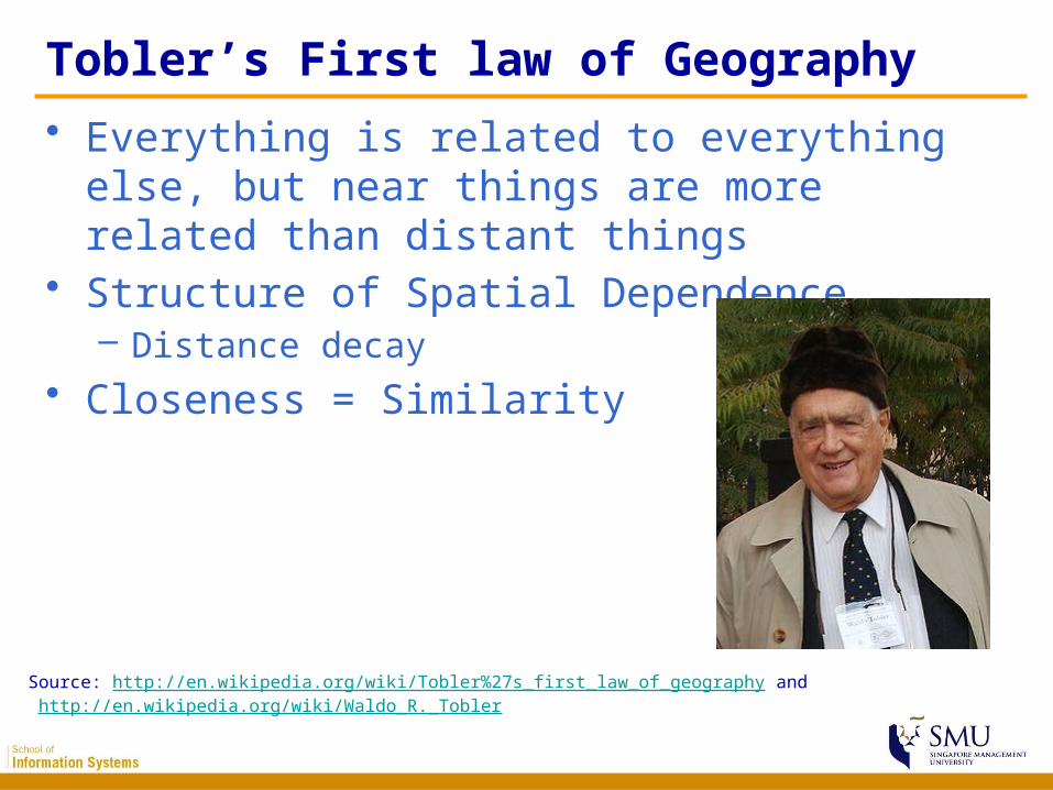
Tobler’s First law of Geography

• Everything is related to everything else, but near things are more related than distant things

• Structure of Spatial Dependence– Distance decay

• Closeness = Similarity

4

Source: http://en.wikipedia.org/wiki/Tobler%27s_first_law_of_geography and http://en.wikipedia.org/wiki/Waldo_R._Tobler

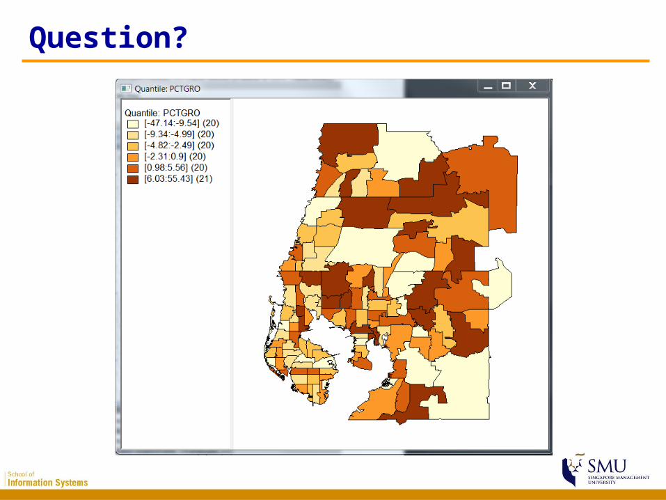
Question?

5

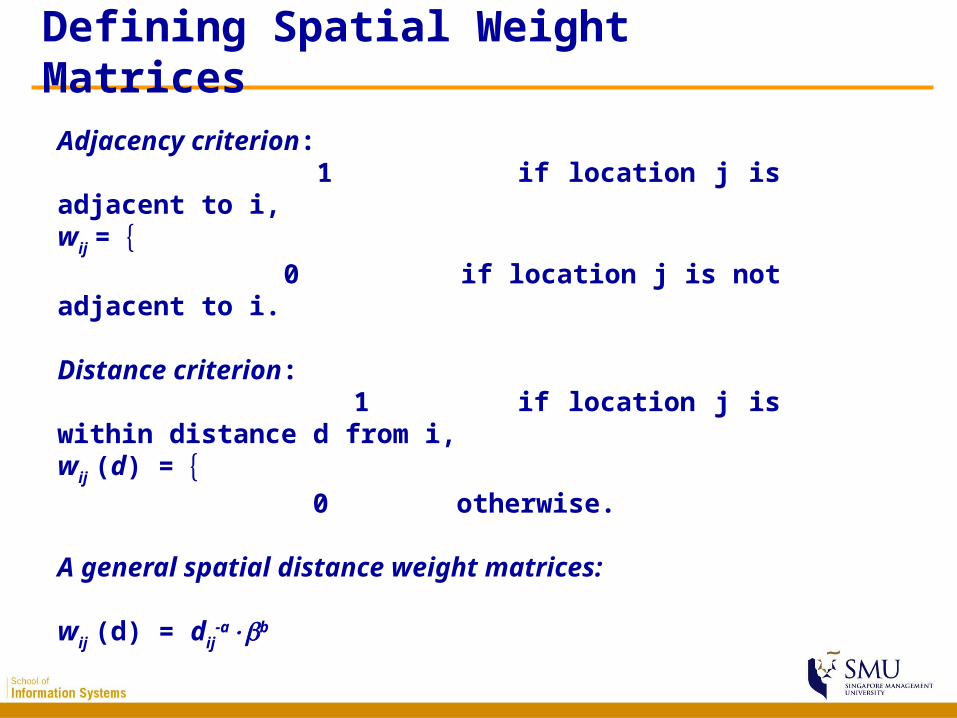
Adjacency criterion: 1 if location j is adjacent to i,wij = 0 if location j is not adjacent to i. Distance criterion: 1 if location j is within distance d from i,wij (d) = 0 otherwise. A general spatial distance weight matrices: wij (d) = dij

-ab

Defining Spatial Weight Matrices

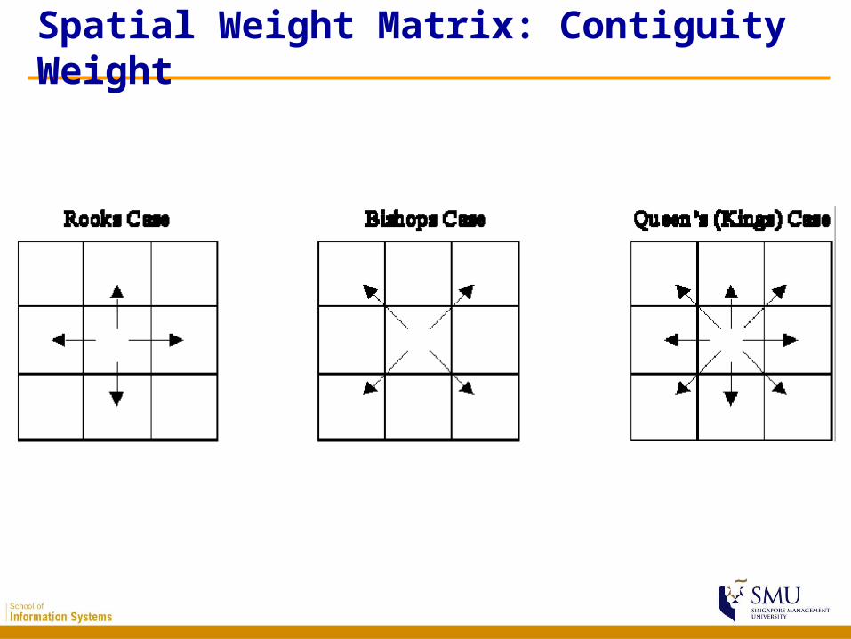
Spatial Weight Matrix: Contiguity Weight

7

I d w x x x x S wij i jj

n

i

n

ijj

n

i

n

( ) ( )( ) ( )

2

Sn

x xii

n2 21

( ) xn

xii

n

11

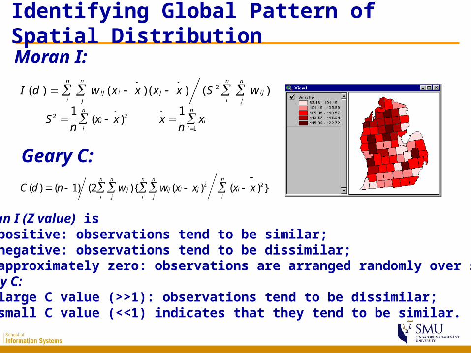
Moran I (Z value) is • positive: observations tend to be similar;• negative: observations tend to be dissimilar;• approximately zero: observations are arranged randomly over space. Geary C:• large C value (>>1): observations tend to be dissimilar;• small C value (<<1) indicates that they tend to be similar.

Moran I:

C d n w w x x x xijj

n

i

n

ij i jj

n

i

n

ii

n

( ) ( ) ( ){ ( ) ( ) }

1 2 2 2

Geary C:

Identifying Global Pattern of Spatial Distribution

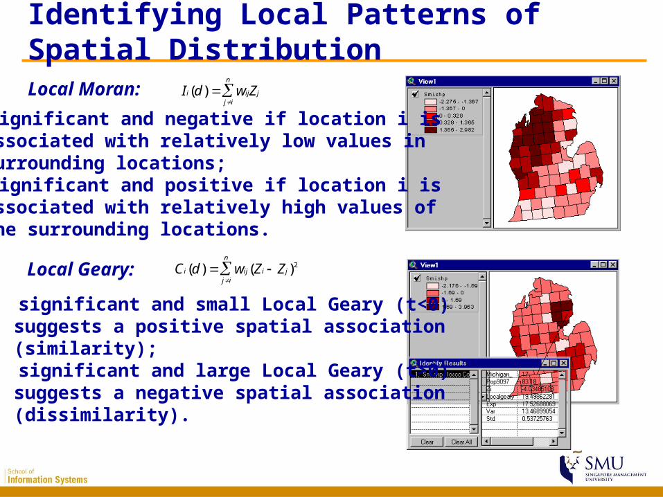
Local Moran: I d w Zi ij jj i

n

( )

Local Geary: C d w Z Zi ij i jj i

n

( ) ( ) 2

• significant and negative if location i is associated with relatively low values in surrounding locations;• significant and positive if location i is associated with relatively high values of the surrounding locations.

• significant and small Local Geary (t<0) suggests a positive spatial association (similarity);• significant and large Local Geary (t>0) suggests a negative spatial association (dissimilarity).

Identifying Local Patterns of Spatial Distribution

Modifiable Areal Unit Problem (MAUP)

• Aggregation Problem– Special case of ecological fallacy– Spatial heterogeneity– A million spatial allocarrelation coefficients

• Zonation Problem– Both in size and spatial arrangement

10

Why do relationships vary spatially?

• Sampling variation– Nuisance variation, not real spatial non-stationarity

• Relationships intrinsically different across space– Real spatial non-stationarity

• Model misspecification– Can significant local variations be removed?

Some definitions

• Spatial non-stationarity: the same stimulus provokes a different response in different parts of the study region

• Global models: statements about processes which are assumed to be stationary and as such are location independent

• Local models: spatial decompositions of global models, the results of local models are location dependent – a characteristic we usually anticipate from geographic (spatial) data

Regression

• Regression establishes relationship among a dependent variable and a set of independent variable(s)

• A typical linear regression model looks like:• yi=0 + 1x1i+ 2x2i+……+ nxni+i

• With yi the dependent variable, xji (j from 1 to n) the set of independent variables, and i the residual, all at location i

• When applied to spatial data, as can be seen, it assumes a stationary spatial process– The same stimulus provokes the same response in all

parts of the study region– Highly untenable for spatial process

Geographically weighted regression• Local statistical technique to analyze spatial

variations in relationships• Spatial non-stationarity is assumed and will be

tested• Based on the “First Law of Geography”: everything

is related with everything else, but closer things are more related

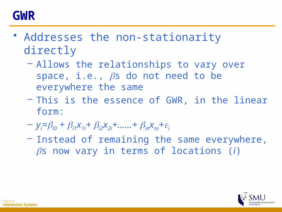
GWR

• Addresses the non-stationarity directly– Allows the relationships to vary over space, i.e., s do

not need to be everywhere the same– This is the essence of GWR, in the linear form:– yi=i0 + i1x1i+ i2x2i+……+ inxni+i

– Instead of remaining the same everywhere, s now vary in terms of locations (i)

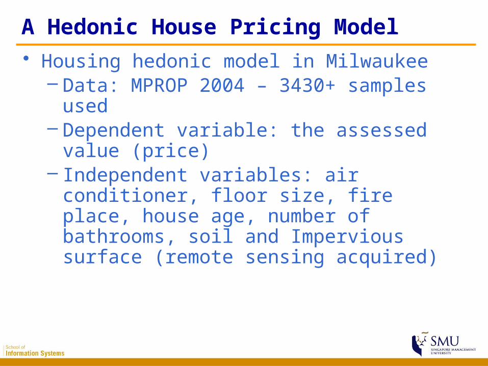
A Hedonic House Pricing Model

• Housing hedonic model in Milwaukee– Data: MPROP 2004 – 3430+ samples used– Dependent variable: the assessed value (price)– Independent variables: air conditioner, floor

size, fire place, house age, number of bathrooms, soil and Impervious surface (remote sensing acquired)

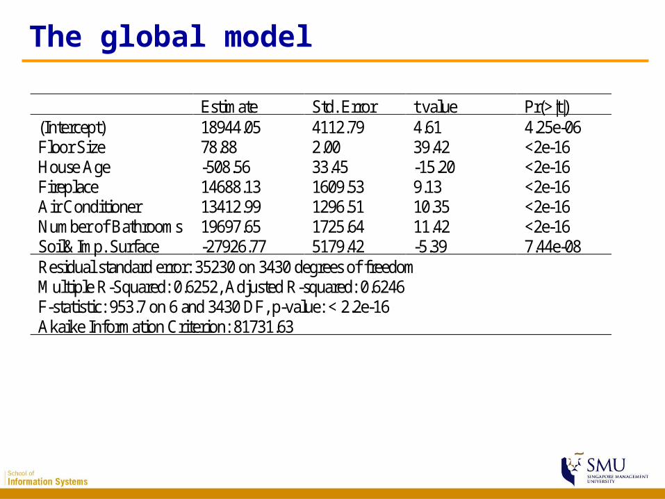
The global model

Estimate Std. Error t value Pr(>|t|) (Intercept) 18944.05 4112.79 4.61 4.25e-06 Floor Size 78.88 2.00 39.42 <2e-16 House Age -508.56 33.45 -15.20 <2e-16 Fireplace 14688.13 1609.53 9.13 <2e-16 Air Conditioner 13412.99 1296.51 10.35 <2e-16 Number of Bathrooms 19697.65 1725.64 11.42 <2e-16 Soil&Imp. Surface -27926.77 5179.42 -5.39 7.44e-08 Residual standard error: 35230 on 3430 degrees of freedom Multiple R-Squared: 0.6252, Adjusted R-squared: 0.6246 F-statistic: 953.7 on 6 and 3430 DF, p-value: < 2.2e-16 Akaike Information Criterion: 81731.63

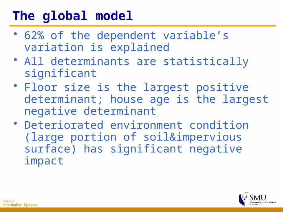
The global model• 62% of the dependent variable’s variation is

explained• All determinants are statistically significant• Floor size is the largest positive determinant;

house age is the largest negative determinant• Deteriorated environment condition (large portion

of soil&impervious surface) has significant negative impact

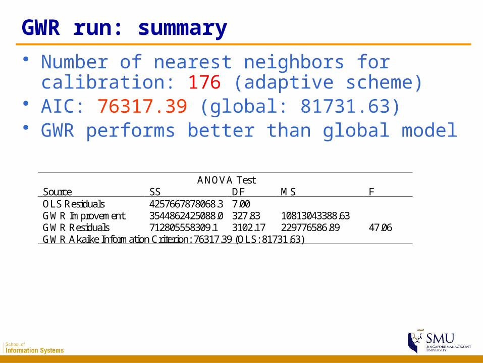
GWR run: summary

• Number of nearest neighbors for calibration: 176 (adaptive scheme)

• AIC: 76317.39 (global: 81731.63)• GWR performs better than global model

ANOVA Test Source SS DF MS F OLS Residuals 4257667878068.3 7.00 GWR Improvement 3544862425088.0 327.83 10813043388.63 GWR Residuals 712805558309.1 3102.17 229776586.89 47.06 GWR Akaike Information Criterion: 76317.39 (OLS: 81731.63)

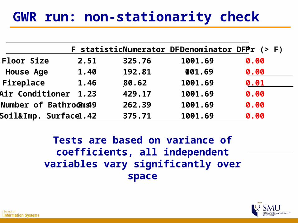
GWR run: non-stationarity check

F statistic Numerator DF Denominator DF* Pr (> F)

Floor Size 2.51 325.76 1001.69 0.00 House Age 1.40 192.81 1001.69 0.00 Fireplace 1.46 80.62 1001.69 0.01 Air Conditioner 1.23 429.17 1001.69 0.00 Number of Bathrooms 2.49 262.39 1001.69 0.00 Soil&Imp. Surface 1.42 375.71 1001.69 0.00

Tests are based on variance of coefficients, all independent variables vary significantly

over space

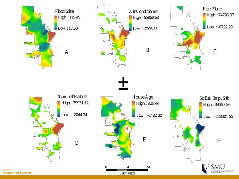
Soil & Imp. SfcHigh : 34357.96

Low : -220301.55

F

House AgeHigh : 929.44

Low : -1402.30

E

Fire PlaceHigh : 74706.97

Low : -6722.29

C

Air ConditionerHigh : 55860.63

Low : -7098.88

B

±

0 10 205

Kilometers

Floor SizeHigh : 119.49

Low : 17.63

A

Num. of BathrmHigh : 39931.12

Low : -2044.24

D

General conclusions

• Except for floor size, the established relationship between house values and the predictors are not necessarily significant everywhere in the City

• Same amount of change in these attributes (ceteris paribus) will bring larger amount of change in house values for houses locate near the Lake than those farther away

General conclusions

• In the northwest and central eastern part of the City, house ages and house values hold opposite relationship as the global model suggests – This is where the original immigrants built their

house, and historical values weight more than house age’s negative impact on house values

Calibration of GWR

• Local weighted least squares– Weights are attached with locations– Based on the “First Law of Geography”:

everything is related with everything else, but closer things are more related than remote ones

Weighting schemes

• Determines weights– Most schemes tend to be Gaussian or

Gaussian-like reflecting the type of dependency found in most spatial processes

– It can be either Fixed or Adaptive– Both schemes based on Gaussian or Gaussian-

like functions are implemented in GWR3.0 and R

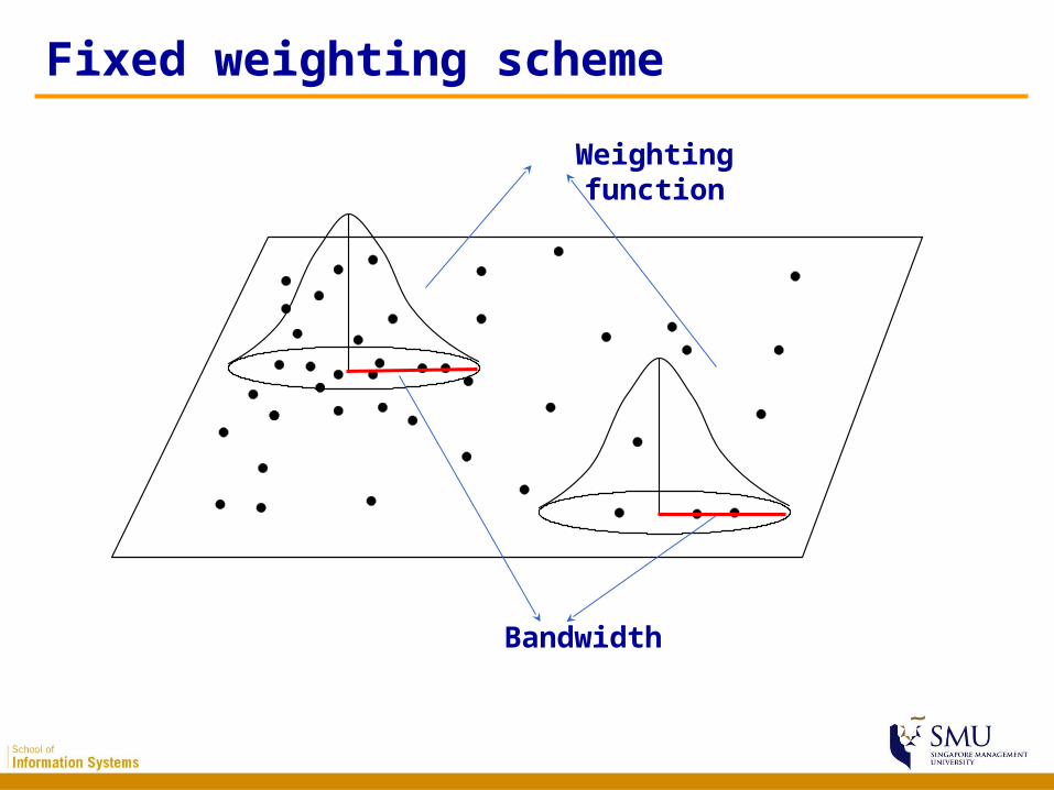
Fixed weighting scheme

Bandwidth

Weighting function

Problems of fixed schemes

• Might produce large estimate variances where data are sparse, while mask subtle local variations where data are dense

• In extreme condition, fixed schemes might not be able to calibrate in local areas where data are too sparse to satisfy the calibration requirements (observations must be more than parameters)

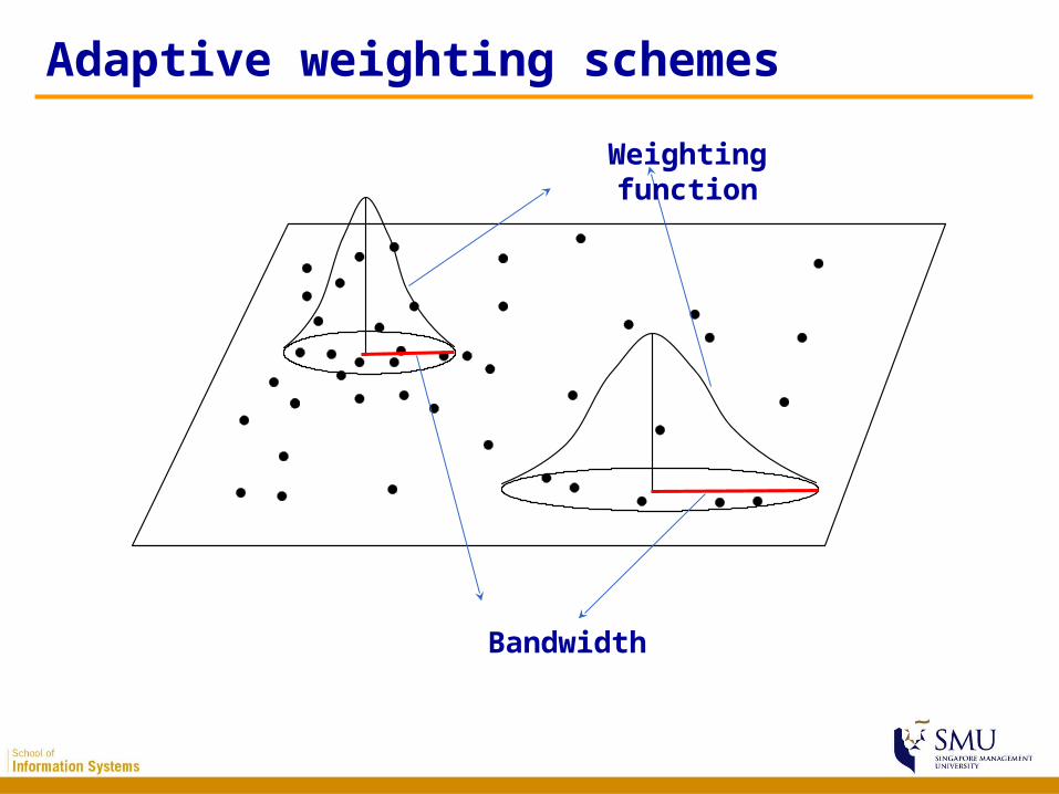
Adaptive weighting schemes

Bandwidth

Weighting function

Adaptive weighting schemes

• Adaptive schemes adjust itself according to the density of data– Shorter bandwidths where data are dense and

longer where sparse– Finding nearest neighbors are one of the often

used approaches

Calibration

• Surprisingly, the results of GWR appear to be relatively insensitive to the choice of weighting functions as long as it is a continuous distance-based function (Gaussian or Gaussian-like functions)

• Whichever weighting function is used, however the result will be sensitive to the bandwidth(s)

Calibration

• An optimal bandwidth (or nearest neighbors) satisfies either– Least cross-validation (CV) score

• CV score: the difference between observed value and the GWR calibrated value using the bandwidth or nearest neighbors

– Least Akaike Information Criterion (AIC)• An information criterion, considers the added

complexity of GWR models