isentropic
DESCRIPTION
IsentropicTRANSCRIPT

Note:
CHAPTER 4: ISENTROPIC
Version: 0.4.8.4 October 8, 2008
This chapter is part of the textbook:º
¹
·
¸
“Fundamentals of Compressible
Flow Mechanics”
You can download the whole book if you like
from: www.potto.org.
This chapter is under GDL with a minor modifi-
cations. Potto License is no longer applied
You should be aware that this book is updated
about every a few weeks or so.
GENICK BAR-MEIR, PH.D.MINNEAPOLIS, MINNESOTA
OCTOBER 8, 2008

THE LIST OF THE AVAILABLE BOOKS IN POTTO PROJECT
ProjectName
Progress Remarks Version
Avail-abilityforPublicDownload
Compressible Flow beta 0.4.8.3 4
Die Casting alpha 0.0.3 4
Dynamics NSY 0.0.0 6
Fluid Mechanics alpha 0.1.8 4
Heat Transfer NSY Based
on
Eckert
0.0.0 6
Mechanics NSY 0.0.0 6
Open Channel
Flow
NSY 0.0.0 6
Statics early
alpha
first
chapter
0.0.1 6
Strength of Material NSY 0.0.0 6
Thermodynamics early
alpha
0.0.01 6
Two/Multi phases
flow
NSY Tel-
Aviv’s
notes
0.0.0 6
NSY = Not Started Yet

CHAPTER 5
Isentropic Flow
distance, x
P
P0
PB = P0
M > 1
Supersonic
SubsonicM < 1
Fig. -5.1: Flow of a compressible substance
(gas) through a converging–
diverging nozzle.
In this chapter a discussion on a steady
state flow through a smooth and con-
tinuous area flow rate is presented.
A discussion about the flow through
a converging–diverging nozzle is also
part of this chapter. The isentropic flow
models are important because of two
main reasons: One, it provides the infor-
mation about the trends and important
parameters. Two, the correction factors
can be introduced later to account for
deviations from the ideal state.
5.1 Stagnation State for
Ideal Gas Model
5.1.1 General Relationship
It is assumed that the flow is one–
dimensional. Figure (5.1) describes a gas flow through a converging–diverging
nozzle. It has been found that a theoretical state known as the stagnation state
is very useful in simplifying the solution and treatment of the flow. The stagnation
state is a theoretical state in which the flow is brought into a complete motionless
condition in isentropic process without other forces (e.g. gravity force). Several
properties that can be represented by this theoretical process which include tem-
perature, pressure, and density et cetera and denoted by the subscript “0.”
49

50 CHAPTER 5. ISENTROPIC FLOW
First, the stagnation temperature is calculated. The energy conservation
can be written as
h +U2
2= h0 (5.1)
Perfect gas is an ideal gas with a constant heat capacity, Cp. For perfect gas
equation (5.1) is simplified into
CpT +U2
2= CpT0 (5.2)
Again it is common to denote T0 as the stagnation temperature. Recalling from
thermodynamic the relationship for perfect gas
R = Cp − Cv (5.3)
and denoting k ≡ Cp ÷ Cv then the thermodynamics relationship obtains the form
Cp =kR
k − 1(5.4)
and where R is a specific constant. Dividing equation (5.2) by (CpT ) yields
1 +U2
2CpT=
T0
T(5.5)
Now, substituting c2 = kRT or T = c2/kR equation (5.5) changes into
1 +kRU2
2Cpc2=
T0
T(5.6)
By utilizing the definition of k by equation (2.24) and inserting it into equation (5.6)
yields
1 +k − 1
2
U2
c2=
T0
T(5.7)
It very useful to convert equation (5.6) into a dimensionless form and de-
note Mach number as the ratio of velocity to speed of sound as
M ≡ U
c(5.8)
Inserting the definition of Mach number (5.8) into equation (5.7) reads
T0
T= 1 +
k − 1
2M2
(5.9)

5.1. STAGNATION STATE FOR IDEAL GAS MODEL 51
velocity
T0
QA B
P0ρ0
T0
P0
ρ0
Fig. -5.2: Perfect gas flows through a tube
The usefulness of Mach num-
ber and equation (5.9) can be demon-
strated by this following simple example.
In this example a gas flows through a
tube (see Figure 5.2) of any shape can
be expressed as a function of only the
stagnation temperature as opposed to
the function of the temperatures and ve-
locities.
The definition of the stagnation state provides the advantage of compact
writing. For example, writing the energy equation for the tube shown in Figure (5.2)
can be reduced to
Q = Cp(T0B − T0A)m (5.10)
The ratio of stagnation pressure to the static pressure can be expressed
as the function of the temperature ratio because of the isentropic relationship as
P0
P=
(T0
T
) kk−1
=
(
1 +k − 1
2M2
) kk−1
(5.11)
In the same manner the relationship for the density ratio is
ρ0
ρ=
(T0
T
) 1k−1
=
(
1 +k − 1
2M2
) 1k−1
(5.12)
A new useful definition is introduced for the case when M = 1 and denoted by
superscript “∗.” The special case of ratio of the star values to stagnation values are
dependent only on the heat ratio as the following:
T ∗
T0=
c∗2
c02
=2
k + 1(5.13)
P ∗
P0=
(2
k + 1
) kk−1
(5.14)
ρ∗
ρ0=
(2
k + 1
) 1k−1
(5.15)

52 CHAPTER 5. ISENTROPIC FLOW
0 1 2 3 4 5 6 7 8 9Mach number
0
0.1
0.2
0.3
0.4
0.5
0.6
0.7
0.8
0.9
1
P/P0
ρ/ρ0T/T
0
Static Properties As A Function of Mach Number
Mon Jun 5 17:39:34 2006
Fig. -5.3: The stagnation properties as a function of the Mach number, k = 1.4
5.1.2 Relationships for Small Mach Number
Even with today’s computers a simplified method can reduce the tedious work in-
volved in computational work. In particular, the trends can be examined with an-
alytical methods. It further will be used in the book to examine trends in derived
models. It can be noticed that the Mach number involved in the above equations
is in a square power. Hence, if an acceptable error is of about %1 then M < 0.1provides the desired range. Further, if a higher power is used, much smaller error
results. First it can be noticed that the ratio of temperature to stagnation tempera-
ture, TT0
is provided in power series. Expanding of the equations according to the
binomial expansion of
(1 + x)n = 1 + nx +n(n − 1)x2
2!+
n(n − 1)(n − 2)x3
3!+ · · · (5.16)
will result in the same fashion
P0
P= 1 +
(k − 1)M2
4+
kM4
8+
2(2 − k)M6
48· · · (5.17)

5.2. ISENTROPIC CONVERGING-DIVERGING FLOW IN CROSS SECTION 53
ρ0
ρ= 1 +
(k − 1)M2
4+
kM4
8+
2(2 − k)M6
48· · · (5.18)
The pressure difference normalized by the velocity (kinetic energy) as correction
factor is
P0 − P12ρU2
= 1 +
compressibility correction︷ ︸︸ ︷
M2
4+
(2 − k)M4
24+ · · · (5.19)
From the above equation, it can be observed that the correction factor approaches
zero when M −→ 0 and then equation (5.19) approaches the standard equation
for incompressible flow.
The definition of the star Mach is ratio of the velocity and star speed of
sound at M = 1.
M∗ =U
c∗=
√
k + 1
2M
(
1 − k − 1
4M2 + · · ·
)
(5.20)
P0 − P
P=
kM2
2
(
1 +M2
4+ · · ·
)
(5.21)
ρ0 − ρ
ρ=
M2
2
(
1 − kM2
4+ · · ·
)
(5.22)
The normalized mass rate becomes
m
A=
√
kP02M2
RT0
(
1 +k − 1
4M2 + · · ·
)
(5.23)
The ratio of the area to star area is
A
A∗=
(2
k + 1
) k+12(k−1)
(1
M+
k + 1
4M +
(3 − k)(k + 1)
32M3 + · · ·
)
(5.24)
5.2 Isentropic Converging-Diverging Flow in Cross Sec-
tion

54 CHAPTER 5. ISENTROPIC FLOW
TρP
U
T+dTρ+dρP+dPU+dU
Fig. -5.4: Control volume inside a converging-
diverging nozzle.
The important sub case in this chap-
ter is the flow in a converging–diverging
nozzle. The control volume is shown
in Figure (5.4). There are two mod-
els that assume variable area flow:
First is isentropic and adiabatic model.
Second is isentropic and isothermal
model. Clearly, the stagnation tem-
perature, T0, is constant through the
adiabatic flow because there isn’t heat
transfer. Therefore, the stagnation pressure is also constant through the flow be-
cause the flow isentropic. Conversely, in mathematical terms, equation (5.9) and
equation (5.11) are the same. If the right hand side is constant for one variable, it
is constant for the other. In the same argument, the stagnation density is constant
through the flow. Thus, knowing the Mach number or the temperature will provide
all that is needed to find the other properties. The only properties that need to be
connected are the cross section area and the Mach number. Examination of the
relation between properties can then be carried out.
5.2.1 The Properties in the Adiabatic Nozzle
When there is no external work and heat transfer, the energy equation, reads
dh + UdU = 0 (5.25)
Differentiation of continuity equation, ρAU = m = constant, and dividing by the
continuity equation reads
dρ
ρ+
dA
A+
dU
U= 0 (5.26)
The thermodynamic relationship between the properties can be expressed as
Tds = dh − dP
ρ(5.27)
For isentropic process ds ≡ 0 and combining equations (5.25) with (5.27) yields
dP
ρ+ UdU = 0 (5.28)
Differentiation of the equation state (perfect gas), P = ρRT , and dividing the
results by the equation of state (ρRT ) yields
dP
P=
dρ
ρ+
dT
T(5.29)
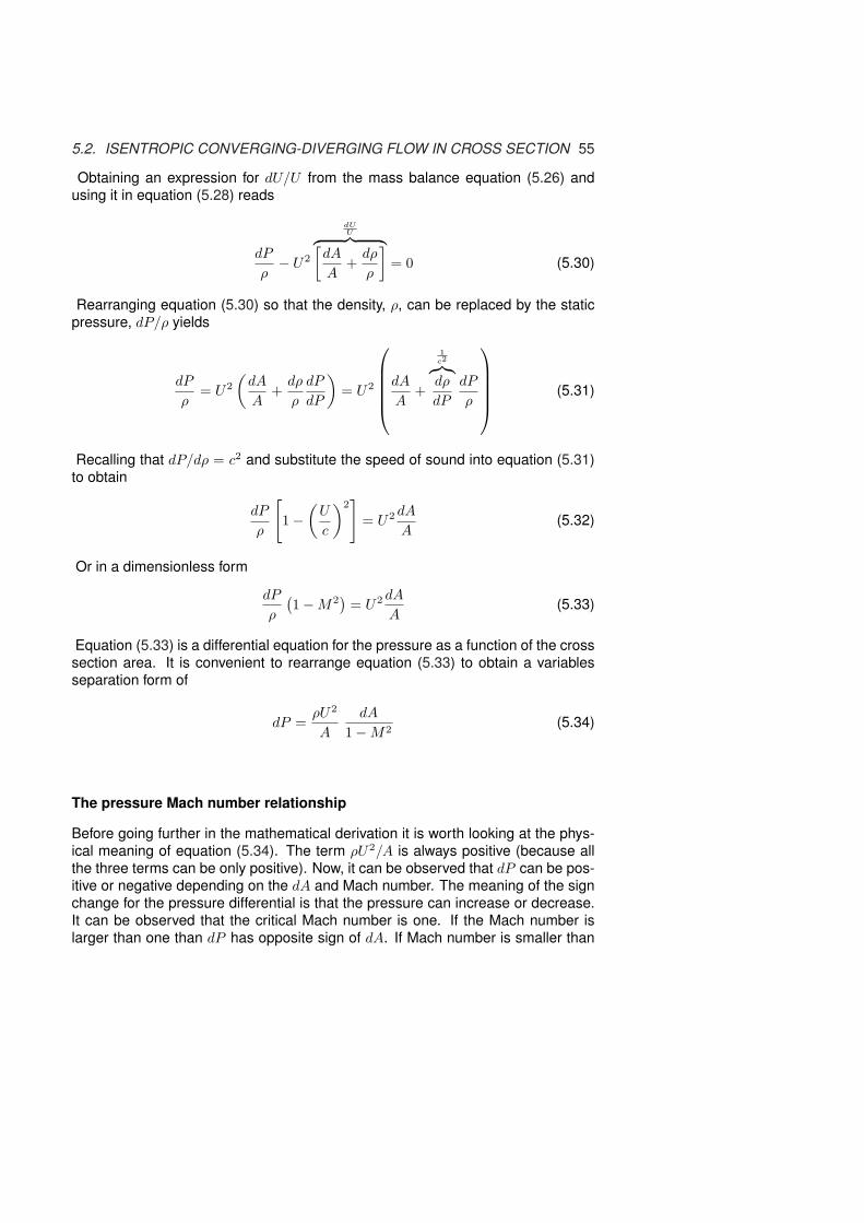
5.2. ISENTROPIC CONVERGING-DIVERGING FLOW IN CROSS SECTION 55
Obtaining an expression for dU/U from the mass balance equation (5.26) and
using it in equation (5.28) reads
dP
ρ− U2
dUU
︷ ︸︸ ︷[dA
A+
dρ
ρ
]
= 0 (5.30)
Rearranging equation (5.30) so that the density, ρ, can be replaced by the static
pressure, dP/ρ yields
dP
ρ= U2
(dA
A+
dρ
ρ
dP
dP
)
= U2
dA
A+
1c2
︷︸︸︷
dρ
dP
dP
ρ
(5.31)
Recalling that dP/dρ = c2 and substitute the speed of sound into equation (5.31)
to obtain
dP
ρ
[
1 −(
U
c
)2]
= U2 dA
A(5.32)
Or in a dimensionless form
dP
ρ
(1 − M2
)= U2 dA
A(5.33)
Equation (5.33) is a differential equation for the pressure as a function of the cross
section area. It is convenient to rearrange equation (5.33) to obtain a variables
separation form of
dP =ρU2
A
dA
1 − M2(5.34)
The pressure Mach number relationship
Before going further in the mathematical derivation it is worth looking at the phys-
ical meaning of equation (5.34). The term ρU2/A is always positive (because all
the three terms can be only positive). Now, it can be observed that dP can be pos-
itive or negative depending on the dA and Mach number. The meaning of the sign
change for the pressure differential is that the pressure can increase or decrease.
It can be observed that the critical Mach number is one. If the Mach number is
larger than one than dP has opposite sign of dA. If Mach number is smaller than

56 CHAPTER 5. ISENTROPIC FLOW
one dP and dA have the same sign. For the subsonic branch M < 1 the term
1/(1 − M2) is positive hence
dA > 0 =⇒ dP > 0
dA < 0 =⇒ dP < 0
From these observations the trends are similar to those in incompressible fluid.
An increase in area results in an increase of the static pressure (converting the
dynamic pressure to a static pressure). Conversely, if the area decreases (as a
function of x) the pressure decreases. Note that the pressure decrease is larger in
compressible flow compared to incompressible flow.
For the supersonic branch M > 1, the phenomenon is different. For M > 1the term 1/1 − M2 is negative and change the character of the equation.
dA > 0 ⇒ dP < 0
dA < 0 ⇒ dP > 0
This behavior is opposite to incompressible flow behavior.
For the special case of M = 1 (sonic flow) the value of the term 1−M2 = 0thus mathematically dP → ∞ or dA = 0. Since physically dP can increase only
in a finite amount it must that dA = 0.It must also be noted that when M = 1occurs only when dA = 0. However, the opposite, not necessarily means that
when dA = 0 that M = 1. In that case, it is possible that dM = 0 thus the diverging
side is in the subsonic branch and the flow isn’t choked.
The relationship between the velocity and the pressure can be observed
from equation (5.28) by solving it for dU .
dU = − dP
PU(5.35)
From equation (5.35) it is obvious that dU has an opposite sign to dP (since the
term PU is positive). Hence the pressure increases when the velocity decreases
and vice versa.
From the speed of sound, one can observe that the density, ρ, increases
with pressure and vice versa (see equation 5.36).
dρ =1
c2dP (5.36)
It can be noted that in the derivations of the above equations (5.35 - 5.36), the
equation of state was not used. Thus, the equations are applicable for any gas
(perfect or imperfect gas).
The second law (isentropic relationship) dictates that ds = 0 and from
thermodynamics
ds = 0 = CpdT
T− R
dP
P

5.2. ISENTROPIC CONVERGING-DIVERGING FLOW IN CROSS SECTION 57
and for perfect gas
dT
T=
k − 1
k
dP
P(5.37)
Thus, the temperature varies according to the same way that pressure does.
The relationship between the Mach number and the temperature can be
obtained by utilizing the fact that the process is assumed to be adiabatic dT0 = 0.
Differentiation of equation (5.9), the relationship between the temperature and the
stagnation temperature becomes
dT0 = 0 = dT
(
1 +k − 1
2M2
)
+ T (k − 1)MdM (5.38)
and simplifying equation (5.38) yields
dT
T= − (k − 1)MdM
1 + k−12 M2
(5.39)
Relationship Between the Mach Number and Cross Section Area
The equations used in the solution are energy (5.39), second law (5.37), state
(5.29), mass (5.26)1. Note, equation (5.33) isn’t the solution but demonstration of
certain properties on the pressure.
The relationship between temperature and the cross section area can be
obtained by utilizing the relationship between the pressure and temperature (5.37)
and the relationship of pressure and cross section area (5.33). First stage equation
(5.39) is combined with equation (5.37) and becomes
(k − 1)
k
dP
P= − (k − 1)MdM
1 + k−12 M2
(5.40)
Combining equation (5.40) with equation (5.33) yields
1
k
ρU2
AdA
1−M2
P= − MdM
1 + k−12 M2
(5.41)
The following identify, ρU2 = kMP can be proved as
kM2P = k
M2
︷︸︸︷
U2
c2
P︷︸︸︷
ρRT = kU2
kRT
P︷︸︸︷
ρRT = ρU2 (5.42)
Using the identity in equation (5.42) changes equation (5.41) into
dA
A=
M2 − 1
M(1 + k−1
2 M2)dM (5.43)
1The momentum equation is not used normally in isentropic process, why?

58 CHAPTER 5. ISENTROPIC FLOW
M, Much nubmer
x
M, A
dAdx = 0 dMdx = 0A,
cross
sectio
n
Fig. -5.5: The relationship between the cross
section and the Mach number on
the subsonic branch
Equation (5.43) is very impor-
tant because it relates the geometry
(area) with the relative velocity (Mach
number). In equation (5.43), the factors
M(1 + k−1
2 M2)
and A are positive re-
gardless of the values of M or A. There-
fore, the only factor that affects relation-
ship between the cross area and the
Mach number is M2 − 1. For M < 1the Mach number is varied opposite to
the cross section area. In the case of
M > 1 the Mach number increases with
the cross section area and vice versa.
The special case is when M = 1 which
requires that dA = 0. This condition
imposes that internal2 flow has to pass
a converting–diverging device to obtain
supersonic velocity. This minimum
area is referred to as “throat.”
Again, the opposite conclusion that when dA = 0 implies that M = 1 is
not correct because possibility of dM = 0. In subsonic flow branch, from the
mathematical point of view: on one hand, a decrease of the cross section increases
the velocity and the Mach number, on the other hand, an increase of the cross
section decreases the velocity and Mach number (see Figure (5.5)).
5.2.2 Isentropic Flow Examples
Example 5.1:
Air is allowed to flow from a reservoir with temperature of 21◦C and with pressure
of 5[MPa] through a tube. It was measured that air mass flow rate is 1[kg/sec]. At
some point on the tube static pressure was measured to be 3[MPa]. Assume that
process is isentropic and neglect the velocity at the reservoir, calculate the Mach
number, velocity, and the cross section area at that point where the static pressure
was measured. Assume that the ratio of specific heat is k = Cp/Cv = 1.4.
SOLUTION
The stagnation conditions at the reservoir will be maintained throughout the tube
because the process is isentropic. Hence the stagnation temperature can be writ-
ten T0 = constant and P0 = constant and both of them are known (the condition at
the reservoir). For the point where the static pressure is known, the Mach number
can be calculated by utilizing the pressure ratio. With the known Mach number,
2This condition does not impose any restrictions for external flow. In external flow, an object can bemoved in arbitrary speed.

5.2. ISENTROPIC CONVERGING-DIVERGING FLOW IN CROSS SECTION 59
the temperature, and velocity can be calculated. Finally, the cross section can be
calculated with all these information.
In the point where the static pressure known
P =P
P0=
3[MPa]
5[MPa]= 0.6
From Table (5.2) or from Figure (5.3) or utilizing the enclosed program, Potto-GDC,
or simply using the equations shows that
MT
T0
ρρ0
A
A⋆P
P0
A×P
A∗×P0
F
F∗
0.88639 0.86420 0.69428 1.0115 0.60000 0.60693 0.53105
With these values the static temperature and the density can be calculated.
T = 0.86420338 × (273 + 21) = 254.076K
ρ =ρ
ρ0
ρ0︷︸︸︷
P0
RT0= 0.69428839 × 5 × 106[Pa]
287.0[
JkgK
]
× 294[K]
= 41.1416
[kg
m3
]
The velocity at that point is
U = M
c︷ ︸︸ ︷√
kRT = 0.88638317 ×√
1.4 × 287 × 294 = 304[m/sec]
The tube area can be obtained from the mass conservation as
A =m
ρU= 8.26 × 10⁻⁵[m3]
For a circular tube the diameter is about 1[cm].
Example 5.2:
The Mach number at point A on tube is measured to be M = 23 and the static pres-
sure is 2[Bar]4. Downstream at point B the pressure was measured to be 1.5[Bar].
Calculate the Mach number at point B under the isentropic flow assumption. Also,
estimate the temperature at point B. Assume that the specific heat ratio k = 1.4and assume a perfect gas model.
4This pressure is about two atmospheres with temperature of 250[K]4Well, this question is for academic purposes, there is no known way for the author to directly mea-
sure the Mach number. The best approximation is by using inserted cone for supersonic flow andmeasure the oblique shock. Here it is subsonic and this technique is not suitable.

60 CHAPTER 5. ISENTROPIC FLOW
SOLUTION
With the known Mach number at point A all the ratios of the static properties to
total (stagnation) properties can be calculated. Therefore, the stagnation pressure
at point A is known and stagnation temperature can be calculated.
At M = 2 (supersonic flow) the ratios are
MT
T0
ρρ0
A
A⋆P
P0
A×P
A∗×P0
F
F∗
2.0000 0.55556 0.23005 1.6875 0.12780 0.21567 0.59309
With this information the pressure at point B can be expressed as
PA
P0=
from the table
5.2 @ M = 2︷︸︸︷
PB
P0×PA
PB= 0.12780453 × 2.0
1.5= 0.17040604
The corresponding Mach number for this pressure ratio is 1.8137788 and TB =0.60315132 PB
P0= 0.17040879. The stagnation temperature can be “bypassed” to
calculate the temperature at point B
TB = TA ×
M=2︷︸︸︷
T0
TA×
M=1.81..︷︸︸︷
TB
T0= 250[K] × 1
0.55555556× 0.60315132 ≃ 271.42[K]
Example 5.3:
Gas flows through a converging–diverging duct. At point “A” the cross section area
is 50 [cm2] and the Mach number was measured to be 0.4. At point B in the duct
the cross section area is 40 [cm2]. Find the Mach number at point B. Assume that
the flow is isentropic and the gas specific heat ratio is 1.4.
SOLUTION
To obtain the Mach number at point B by finding the ratio of the area to the critical
area. This relationship can be obtained by
AB
A∗ =AB
AA× AA
A∗=
40
50×
from the Table 5.2︷ ︸︸ ︷
1.59014 = 1.272112
With the value of AB
A∗from the Table (5.2) or from Potto-GDC two solutions can
be obtained. The two possible solutions: the first supersonic M = 1.6265306 and
second subsonic M = 0.53884934. Both solution are possible and acceptable. The
supersonic branch solution is possible only if there where a transition at throat
where M=1.

5.2. ISENTROPIC CONVERGING-DIVERGING FLOW IN CROSS SECTION 61
MT
T0
ρρ0
A
A⋆P
P0
A×P
A∗×P0
1.6266 0.65396 0.34585 1.2721 0.22617 0.287720.53887 0.94511 0.86838 1.2721 0.82071 1.0440
Example 5.4:
Engineer needs to redesign a syringe for medical applications. The complain in
the syringe is that the syringe is “hard to push.” The engineer analyzes the flow
and conclude that the flow is choke. Upon this fact, what engineer should do with
syringe increase the pushing diameter or decrease the diameter? Explain.
SOLUTION
This problem is a typical to compressible flow in the sense the solution is opposite
the regular intuition. The diameter should be decreased. The pressure in the choke
flow in the syringe is past the critical pressure ratio. Hence, the force is a function
of the cross area of the syringe. So, to decrease the force one should decrease
the area.
End Solution
5.2.3 Mass Flow Rate (Number)
One of the important engineering parameters is the mass flow rate which for ideal
gas is
m = ρUA =P
RTUA (5.44)
This parameter is studied here, to examine the maximum flow rate and to see what
is the effect of the compressibility on the flow rate. The area ratio as a function of
the Mach number needed to be established, specifically and explicitly the relation-
ship for the chocked flow. The area ratio is defined as the ratio of the cross section
at any point to the throat area (the narrow area). It is convenient to rearrange the
equation (5.44) to be expressed in terms of the stagnation properties as
m
A=
P
P0
P0U√kRT
√
k
R
√
T0
T
1√T0
=P0√T0
M
√
k
R
f(M,k)︷ ︸︸ ︷
P
P0
√
T0
T(5.45)
Expressing the temperature in terms of Mach number in equation (5.45) results
in
m
A=
(kMP0√kRT0
)(
1 +k − 1
2M2
)−
k+12(k−1)
(5.46)
It can be noted that equation (5.46) holds everywhere in the converging-diverging
duct and this statement also true for the throat. The throat area can be denoted
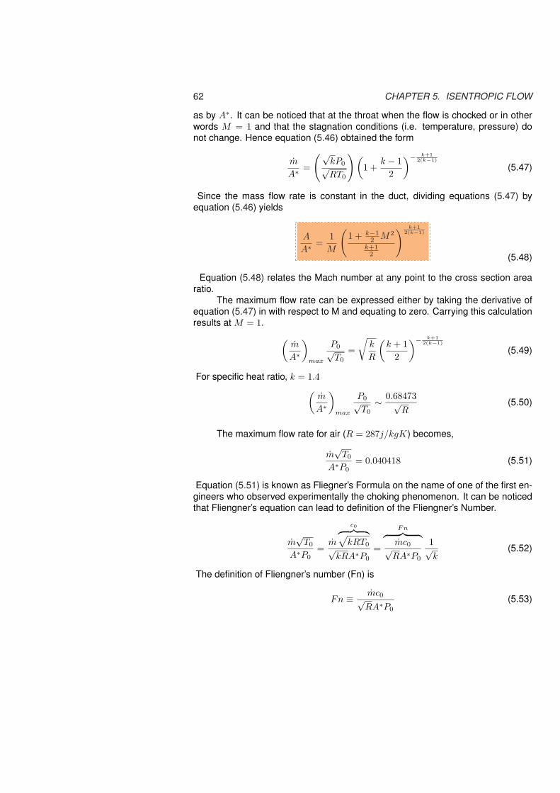
62 CHAPTER 5. ISENTROPIC FLOW
as by A∗. It can be noticed that at the throat when the flow is chocked or in other
words M = 1 and that the stagnation conditions (i.e. temperature, pressure) do
not change. Hence equation (5.46) obtained the form
m
A∗=
(√kP0√RT0
) (
1 +k − 1
2
)−
k+12(k−1)
(5.47)
Since the mass flow rate is constant in the duct, dividing equations (5.47) by
equation (5.46) yields
A
A∗=
1
M
(
1 + k−12 M2
k+12
) k+12(k−1)
(5.48)
Equation (5.48) relates the Mach number at any point to the cross section area
ratio.
The maximum flow rate can be expressed either by taking the derivative of
equation (5.47) in with respect to M and equating to zero. Carrying this calculation
results at M = 1.
(m
A∗
)
max
P0√T0
=
√
k
R
(k + 1
2
)−
k+12(k−1)
(5.49)
For specific heat ratio, k = 1.4
(m
A∗
)
max
P0√T0
∼ 0.68473√R
(5.50)
The maximum flow rate for air (R = 287j/kgK) becomes,
m√
T0
A∗P0= 0.040418 (5.51)
Equation (5.51) is known as Fliegner’s Formula on the name of one of the first en-
gineers who observed experimentally the choking phenomenon. It can be noticed
that Fliengner’s equation can lead to definition of the Fliengner’s Number.
m√
T0
A∗P0=
m
c0︷ ︸︸ ︷√
kRT0√kRA∗P0
=
Fn︷ ︸︸ ︷
mc0√RA∗P0
1√k
(5.52)
The definition of Fliengner’s number (Fn) is
Fn ≡ mc0√RA∗P0
(5.53)

5.2. ISENTROPIC CONVERGING-DIVERGING FLOW IN CROSS SECTION 63
Utilizing Fliengner’s number definition and substituting it into equation (5.47)
results in
Fn = kM
(
1 +k − 1
2M2
)−
k+12(k−1)
(5.54)
and the maximum point for Fn at M = 1 is
Fn = k
(k + 1
2
)−
k+12(k−1)
(5.55)
“Naughty Professor” Problems in Isentropic Flow
To explain the material better some instructors invented problems, which have
mostly academic purpose, (see for example, Shapiro (problem 4.5)). While these
problems have a limit applicability in reality, they have substantial academic value
and therefore presented here. The situation where the mass flow rate per area
given with one of the stagnation properties and one of the static properties, e.g.
P0 and T or T0 and P present difficulty for the calculations. The use of the regu-
lar isentropic Table is not possible because there isn’t variable represent this kind
problems. For this kind of problems a new Table was constructed and present
here5.
The case of T0 and PThis case considered to be simplest case and will first presented here. Using
energy equation (5.9) and substituting for Mach number M = m/Aρc results in
T0
T= 1 +
k − 1
2
(m
Aρc
)2
(5.56)
Rearranging equation (5.56) result in
T0ρ2 =
pR
︷︸︸︷
Tρ ρ +
1/kR︷ ︸︸ ︷(
T
c2
)k − 1
2
(m
A
)2
(5.57)
And further Rearranging equation (5.57) transformed it into
ρ2 =Pρ
T0R+
k − 1
2kRT0
(m
A
)2
(5.58)
5Since version 0.44 of this book.

64 CHAPTER 5. ISENTROPIC FLOW
Equation (5.58) is quadratic equation for density, ρ when all other variables are
known. It is convenient to change it into
ρ2 − Pρ
T0R− k − 1
2kRT0
(m
A
)2
= 0 (5.59)
The only physical solution is when the density is positive and thus the only solution
is
ρ =1
2
P
RT0+
√√√√√√
(P
RT0
)2
+ 2k − 1
kRT0
(m
A
)2
︸ ︷︷ ︸
→(M→0)→0
(5.60)
For almost incompressible flow the density is reduced and the familiar form of
perfect gas model is seen since stagnation temperature is approaching the static
temperature for very small Mach number (ρ = PRT0
). In other words, the terms
for the group over the under–brace approaches zero when the flow rate (Mach
number) is very small.
It is convenient to denote a new dimensionless density as
ρ =ρp
RT0
=ρRT0
P=
1
T(5.61)
With this new definition equation (5.60) is transformed into
ρ =1
2
1 +
√
1 + 2(k − 1)RT0
kP 2
(m
A
)2
(5.62)
The dimensionless density now is related to a dimensionless group that is a func-
tion of Fn number and Mach number only! Thus, this dimensionless group is func-
tion of Mach number only.
RT0
P 2
(m
A
)2
=1
k
Fn2
︷ ︸︸ ︷
c02
P02
(m
A∗
)2
A∗P0AP
=f(M)︷ ︸︸ ︷(
A∗
A
)2 (P0
P
)2
(5.63)
Thus,
RT0
P 2
(m
A
)2
=Fn2
k
(A∗P0
AP
)2
(5.64)
Hence, the dimensionless density is
ρ =1
2
1 +
√
1 + 2(k − 1)Fn2
k2
(A∗P0
AP
)2
(5.65)

5.2. ISENTROPIC CONVERGING-DIVERGING FLOW IN CROSS SECTION 65
Again notice that the right hand side of equation (5.65) is only function of Mach
number (well, also the specific heat, k). And the values of APA∗P0
were tabulated
in Table (5.2) and Fn is tabulated in the next Table (5.1). Thus, the problems is
reduced to finding tabulated values.
The case of P0 and T
A similar problem can be described for the case of stagnation pressure, P0,
and static temperature, T .
First, it is shown that the dimensionless group is a function of Mach number
only (well, again the specific heat ratio, k also).
RT
P02
(m
A
)2
=Fn2
k
(A∗P0
AP
)2 (T
T0
)(P0
P
)2
(5.66)
It can be noticed that
Fn2
k=
(T
T0
)(P0
P
)2
(5.67)
Thus equation (5.66) became
RT
P02
(m
A
)2
=
(A∗P0
AP
)2
(5.68)
The right hand side is tabulated in the “regular” isentropic Table such (5.2). This
example shows how a dimensional analysis is used to solve a problems without
actually solving any equations. The actual solution of the equation is left as ex-
ercise (this example under construction). What is the legitimacy of this method?
The explanation simply based the previous experience in which for a given ratio of
area or pressure ratio (etcetera) determines the Mach number. Based on the same
arguments, if it was shown that a group of parameters depends only Mach number
than the Mach is determined by this group.
The method of solution for given these parameters is by calculating the PAP0A∗
and then using the table to find the corresponding Mach number.
The case of ρ0 and T or P
The last case sometimes referred to as the “naughty professor’s question” case
dealt here is when the stagnation density given with the static temperature/pressure.
First, the dimensionless approach is used later analytical method is discussed (un-
der construction).
1
Rρ0P
(m
A
)2
=
c02
︷ ︸︸ ︷
kRT0
kRP0P0PP0
(m
A
)2
=c0
2
kRP02 P
P0
(m
A
)2
=Fn2
k
(P0
P
)
(5.69)

66 CHAPTER 5. ISENTROPIC FLOW
The last case dealt here is of the stagnation density with static pressure and the
following is dimensionless group
1
Rρ02T
(m
A
)2
=
c02
︷ ︸︸ ︷
kRT0 T0
kRP02T
(m
A
)2
=c0
2T0
kRP02T
(m
A
)2
=Fn2
k
(T0
T
)
(5.70)
It was hidden in the derivations/explanations of the above analysis didn’t explic-
itly state under what conditions these analysis is correct. Unfortunately, not all the
analysis valid for the same conditions and is as the regular “isentropic” Table, (5.2).
The heat/temperature part is valid for enough adiabatic condition while the pres-
sure condition requires also isentropic process. All the above conditions/situations
require to have the perfect gas model as the equation of state. For example the
first “naughty professor” question is sufficient that process is adiabatic only (T0, P ,
mass flow rate per area.).
Table -5.1: Fliegner’s number and other parameters as a function of Mach number
M Fn ρ(
P0A∗
AP
)2RT0
P2
(m
A
)2 1
Rρ0P
(m
A
)2 1
Rρ02T
(m
A
)2
0.00E+001.400E−061.000 0.0 0.0 0.0 0.00.050001 0.070106 1.000 0.00747 2.62E−05 0.00352 0.003510.10000 0.14084 1.000 0.029920 0.000424 0.014268 0.0141970.20000 0.28677 1.001 0.12039 0.00707 0.060404 0.0592120.21000 0.30185 1.001 0.13284 0.00865 0.067111 0.0656540.22000 0.31703 1.001 0.14592 0.010476 0.074254 0.0724870.23000 0.33233 1.002 0.15963 0.012593 0.081847 0.0797220.24000 0.34775 1.002 0.17397 0.015027 0.089910 0.0873720.25000 0.36329 1.003 0.18896 0.017813 0.098460 0.0954490.26000 0.37896 1.003 0.20458 0.020986 0.10752 0.103970.27000 0.39478 1.003 0.22085 0.024585 0.11710 0.112940.28000 0.41073 1.004 0.23777 0.028651 0.12724 0.122390.29000 0.42683 1.005 0.25535 0.033229 0.13796 0.132320.30000 0.44309 1.005 0.27358 0.038365 0.14927 0.142760.31000 0.45951 1.006 0.29247 0.044110 0.16121 0.153720.32000 0.47609 1.007 0.31203 0.050518 0.17381 0.165220.33000 0.49285 1.008 0.33226 0.057647 0.18709 0.177280.34000 0.50978 1.009 0.35316 0.065557 0.20109 0.189920.35000 0.52690 1.011 0.37474 0.074314 0.21584 0.203160.36000 0.54422 1.012 0.39701 0.083989 0.23137 0.217030.37000 0.56172 1.013 0.41997 0.094654 0.24773 0.231550.38000 0.57944 1.015 0.44363 0.10639 0.26495 0.246740.39000 0.59736 1.017 0.46798 0.11928 0.28307 0.262640.40000 0.61550 1.019 0.49305 0.13342 0.30214 0.27926

5.2. ISENTROPIC CONVERGING-DIVERGING FLOW IN CROSS SECTION 67
Table -5.1: Fliegner’s number and other parameters as function of Mach number (continue)
M Fn ρ(
P0A∗
AP
)2RT0
P2
(m
A
)2 1
Rρ0P
(m
A
)2 1
Rρ02T
(m
A
)2
0.41000 0.63386 1.021 0.51882 0.14889 0.32220 0.296630.42000 0.65246 1.023 0.54531 0.16581 0.34330 0.314800.43000 0.67129 1.026 0.57253 0.18428 0.36550 0.333780.44000 0.69036 1.028 0.60047 0.20442 0.38884 0.353610.45000 0.70969 1.031 0.62915 0.22634 0.41338 0.374320.46000 0.72927 1.035 0.65857 0.25018 0.43919 0.395960.47000 0.74912 1.038 0.68875 0.27608 0.46633 0.418550.48000 0.76924 1.042 0.71967 0.30418 0.49485 0.442150.49000 0.78965 1.046 0.75136 0.33465 0.52485 0.466770.50000 0.81034 1.050 0.78382 0.36764 0.55637 0.492490.51000 0.83132 1.055 0.81706 0.40333 0.58952 0.519320.52000 0.85261 1.060 0.85107 0.44192 0.62436 0.547330.53000 0.87421 1.065 0.88588 0.48360 0.66098 0.576560.54000 0.89613 1.071 0.92149 0.52858 0.69948 0.607060.55000 0.91838 1.077 0.95791 0.57709 0.73995 0.638890.56000 0.94096 1.083 0.99514 0.62936 0.78250 0.672100.57000 0.96389 1.090 1.033 0.68565 0.82722 0.706750.58000 0.98717 1.097 1.072 0.74624 0.87424 0.742900.59000 1.011 1.105 1.112 0.81139 0.92366 0.780620.60000 1.035 1.113 1.152 0.88142 0.97562 0.819960.61000 1.059 1.122 1.194 0.95665 1.030 0.861010.62000 1.084 1.131 1.236 1.037 1.088 0.903820.63000 1.109 1.141 1.279 1.124 1.148 0.948480.64000 1.135 1.151 1.323 1.217 1.212 0.995070.65000 1.161 1.162 1.368 1.317 1.278 1.0440.66000 1.187 1.173 1.414 1.423 1.349 1.0940.67000 1.214 1.185 1.461 1.538 1.422 1.1470.68000 1.241 1.198 1.508 1.660 1.500 1.2020.69000 1.269 1.211 1.557 1.791 1.582 1.2600.70000 1.297 1.225 1.607 1.931 1.667 1.3200.71000 1.326 1.240 1.657 2.081 1.758 1.3820.72000 1.355 1.255 1.708 2.241 1.853 1.4480.73000 1.385 1.271 1.761 2.412 1.953 1.5160.74000 1.415 1.288 1.814 2.595 2.058 1.5870.75000 1.446 1.305 1.869 2.790 2.168 1.6610.76000 1.477 1.324 1.924 2.998 2.284 1.7380.77000 1.509 1.343 1.980 3.220 2.407 1.8190.78000 1.541 1.362 2.038 3.457 2.536 1.9030.79000 1.574 1.383 2.096 3.709 2.671 1.991

68 CHAPTER 5. ISENTROPIC FLOW
Table -5.1: Fliegner’s number and other parameters as function of Mach number (continue)
M Fn ρ(
P0A∗
AP
)2RT0
P2
(m
A
)2 1
Rρ0P
(m
A
)2 1
Rρ02T
(m
A
)2
0.80000 1.607 1.405 2.156 3.979 2.813 2.0820.81000 1.642 1.427 2.216 4.266 2.963 2.1770.82000 1.676 1.450 2.278 4.571 3.121 2.2770.83000 1.712 1.474 2.340 4.897 3.287 2.3810.84000 1.747 1.500 2.404 5.244 3.462 2.4890.85000 1.784 1.526 2.469 5.613 3.646 2.6020.86000 1.821 1.553 2.535 6.006 3.840 2.7200.87000 1.859 1.581 2.602 6.424 4.043 2.8420.88000 1.898 1.610 2.670 6.869 4.258 2.9710.89000 1.937 1.640 2.740 7.342 4.484 3.1040.90000 1.977 1.671 2.810 7.846 4.721 3.2440.91000 2.018 1.703 2.882 8.381 4.972 3.3890.92000 2.059 1.736 2.955 8.949 5.235 3.5410.93000 2.101 1.771 3.029 9.554 5.513 3.6990.94000 2.144 1.806 3.105 10.20 5.805 3.8650.95000 2.188 1.843 3.181 10.88 6.112 4.0370.96000 2.233 1.881 3.259 11.60 6.436 4.2170.97000 2.278 1.920 3.338 12.37 6.777 4.4040.98000 2.324 1.961 3.419 13.19 7.136 4.6000.99000 2.371 2.003 3.500 14.06 7.515 4.8041.000 2.419 2.046 3.583 14.98 7.913 5.016
Example 5.5:
A gas flows in the tube with mass flow rate of 0.1 [kg/sec] and tube cross section
is 0.001[m2]. The temperature at Chamber supplying the pressure to tube is 27◦C.
At some point the static pressure was measured to be 1.5[Bar]. Calculate for that
point the Mach number, the velocity, and the stagnation pressure. Assume that the
process is isentropic, k = 1.3, R = 287[j/kgK].
SOLUTION
The first thing that need to be done is to find the mass flow per area and it is
m
A= 0.1/0.001 = 100.0[kg/sec/m2]
It can be noticed that the total temperature is 300K and the static pressure is
1.5[Bar]. The solution is based on section equations (5.60) through (5.65). It is
fortunate that Potto-GDC exist and it can be just plug into it and it provide that
MT
T0
ρρ0
A
A⋆P
P0
A×P
A∗×P0
F
F∗
0.17124 0.99562 0.98548 3.4757 0.98116 3.4102 1.5392

5.2. ISENTROPIC CONVERGING-DIVERGING FLOW IN CROSS SECTION 69
The velocity can be calculated as
U = Mc =√
kRTM = 0.17 ×√
1.3 × 287 × 300× ∼ 56.87[m/sec]
The stagnation pressure is
P0 =P
P/P0= 1.5/0.98116 = 1.5288[Bar]
Flow with pressure losses
The expression for the mass flow rate (5.46) is appropriate regardless the flow is
isentropic or adiabatic. That expression was derived based on the theoretical total
pressure and temperature (Mach number) which does not based on the considera-
tions whether the flow is isentropic or adiabatic. In the same manner the definition
of A∗ referred to the theoretical minimum area (”throat area”) if the flow continues
to flow in an isentropic manner. Clearly, in a case where the flow isn’t isentropic or
adiabatic the total pressure and the total temperature will change (due to friction,
and heat transfer). A constant flow rate requires that mA = mB . Denoting sub-
script A for one point and subscript B for another point mass equation (5.47) can
be equated as
(kP0A
∗
RT0
)(
1 +k − 1
2M2
)−
k−12(k−1)
= constant (5.71)
From equation (5.71), it is clear that the function f(P0, T0, A∗) = constant. There
are two possible models that can be used to simplify the calculations. The first
model for neglected heat transfer (adiabatic) flow and in which the total temperature
remained constant (Fanno flow like). The second model which there is significant
heat transfer but insignificant pressure loss (Rayleigh flow like).
If the mass flow rate is constant at any point on the tube (no mass loss occur) then
m = A∗
√
k
RT0
(2
k + 1
) k+1k−1
P0 (5.72)
For adiabatic flow, comparison of mass flow rate at point A and point B leads to
P0A∗|A = P0A
∗|B
;
P0|AP0|B
=A∗|AA∗|B
(5.73)
And utilizing the equality of A∗ = A∗
A A leads to
P0|AP0|B
=
AA∗
∣∣MA
AA∗
∣∣MB
A|AA|B
(5.74)

70 CHAPTER 5. ISENTROPIC FLOW
For a flow with a constant stagnation pressure (frictionless flow) and non adiabatic
flow reads
T0|AT0|B
=
[BA∗
∣∣MB
AA∗
∣∣MA
A|BA|A
]2
(5.75)
Example 5.6:
At point A of the tube the pressure is 3[Bar], Mach number is 2.5, and the duct
section area is 0.01[m2]. Downstream at exit of tube, point B, the cross section
area is 0.015[m2] and Mach number is 1.5. Assume no mass lost and adiabatic
steady state flow, calculated the total pressure lost.
SOLUTION
Both Mach numbers are known, thus the area ratios can be calculated. The to-
tal pressure can be calculated because the Mach number and static pressure are
known. With these information, and utilizing equation (5.74) the stagnation pres-
sure at point B can be obtained.
MT
T0
ρρ0
A
A⋆P
P0
A×P
A∗×P0
F
F∗
1.5000 0.68966 0.39498 1.1762 0.27240 0.32039 0.554012.5000 0.44444 0.13169 2.6367 0.05853 0.15432 0.62693
First, the stagnation at point A is obtained from Table (5.2) as
P0|A =P
(P
P0
)
︸ ︷︷ ︸
M=2.5
∣∣∣∣∣∣∣∣∣∣∣∣∣A
=3
0.058527663= 51.25781291[Bar]
by utilizing equation (5.74) provides
P0|B = 51.25781291 × 1.1761671
2.6367187× 0.01
0.015≈ 15.243[Bar]
Hence
P0|A − P0|B = 51.257 − 15.243 = 36.013[Bar]
Note that the large total pressure loss is much larger than the static pressure loss
(Pressure point B the pressure is 0.27240307 × 15.243 = 4.146[Bar]).
5.3 Isentropic Tables

5.3. ISENTROPIC TABLES 71
Table -5.2: Isentropic Table k = 1.4
MT
T0
ρρ0
A
A⋆P
P0
A×P
A∗×P0
F
F∗
0.000 1.00000 1.00000 5.8E+5 1.0000 5.8E + 5 2.4E+50.050 0.99950 0.99875 11.59 0.99825 11.57 4.8380.100 0.99800 0.99502 5.822 0.99303 5.781 2.4430.200 0.99206 0.98028 2.964 0.97250 2.882 1.2680.300 0.98232 0.95638 2.035 0.93947 1.912 0.896990.400 0.96899 0.92427 1.590 0.89561 1.424 0.726320.500 0.95238 0.88517 1.340 0.84302 1.130 0.635350.600 0.93284 0.84045 1.188 0.78400 0.93155 0.583770.700 0.91075 0.79158 1.094 0.72093 0.78896 0.554250.800 0.88652 0.73999 1.038 0.65602 0.68110 0.538070.900 0.86059 0.68704 1.009 0.59126 0.59650 0.530391.00 0.83333 0.63394 1.000 0.52828 0.52828 0.528281.100 0.80515 0.58170 1.008 0.46835 0.47207 0.529891.200 0.77640 0.53114 1.030 0.41238 0.42493 0.533991.300 0.74738 0.48290 1.066 0.36091 0.38484 0.539741.400 0.71839 0.43742 1.115 0.31424 0.35036 0.546551.500 0.68966 0.39498 1.176 0.27240 0.32039 0.554011.600 0.66138 0.35573 1.250 0.23527 0.29414 0.561821.700 0.63371 0.31969 1.338 0.20259 0.27099 0.569761.800 0.60680 0.28682 1.439 0.17404 0.25044 0.577681.900 0.58072 0.25699 1.555 0.14924 0.23211 0.585492.000 0.55556 0.23005 1.688 0.12780 0.21567 0.593092.500 0.44444 0.13169 2.637 0.058528 0.15432 0.626933.000 0.35714 0.076226 4.235 0.027224 0.11528 0.653263.500 0.28986 0.045233 6.790 0.013111 0.089018 0.673204.000 0.23810 0.027662 10.72 0.00659 0.070595 0.688304.500 0.19802 0.017449 16.56 0.00346 0.057227 0.699835.000 0.16667 0.011340 25.00 0.00189 0.047251 0.708765.500 0.14184 0.00758 36.87 0.00107 0.039628 0.715786.000 0.12195 0.00519 53.18 0.000633 0.033682 0.721366.500 0.10582 0.00364 75.13 0.000385 0.028962 0.725867.000 0.092593 0.00261 1.0E+2 0.000242 0.025156 0.729537.500 0.081633 0.00190 1.4E+2 0.000155 0.022046 0.732578.000 0.072464 0.00141 1.9E+2 0.000102 0.019473 0.735108.500 0.064725 0.00107 2.5E+2 6.90E−5 0.017321 0.737239.000 0.058140 0.000815 3.3E+2 4.74E−5 0.015504 0.739039.500 0.052493 0.000631 4.2E+2 3.31E−5 0.013957 0.74058
10.00 0.047619 0.000495 5.4E+2 2.36E−5 0.012628 0.74192

72 CHAPTER 5. ISENTROPIC FLOW
5.3.1 Isentropic Isothermal Flow Nozzle
5.3.2 General Relationship
In this section, the other extreme case model where the heat transfer to the gas
is perfect, (e.g. Eckert number is very small) is presented. Again in reality the
heat transfer is somewhere in between the two extremes. So, knowing the two
limits provides a tool to examine where the reality should be expected. The perfect
gas model is again assumed (later more complex models can be assumed and
constructed in a future versions). In isothermal process the perfect gas model
reads
P = ρRT ; dP = dρRT (5.76)
Substituting equation (5.76) into the momentum equation6 yields
UdU +RTdP
P= 0 (5.77)
Integration of equation (5.77) yields the Bernoulli’s equation for ideal gas in isother-
mal process which reads
;
U22 − U1
2
2+ RT ln
P2
P1= 0 (5.78)
Thus, the velocity at point 2 becomes
U2 =
√
2RT lnP2
P1− U1
2 (5.79)
The velocity at point 2 for stagnation point, U1 ≈ 0 reads
U2 =
√
2RT lnP2
P1(5.80)
Or in explicit terms of the stagnation properties the velocity is
U =
√
2RT lnP
P0(5.81)
Transform from equation (5.78) to a dimensionless form becomes
;
kR¡¡µconstant
T (M22 − M1
2)
2= R¡¡µ
constant
T lnP2
P1(5.82)
6The one dimensional momentum equation for steady state is UdU/dx = −dP/dx+0(other effects)which are neglected here.

5.3. ISENTROPIC TABLES 73
Simplifying equation (5.82) yields
;
k(M22 − M1
2)
2= ln
P2
P1(5.83)
Or in terms of the pressure ratio equation (5.83) reads
P2
P1= e
k(M12−M2
2)2 =
(
eM12
eM22
) k2
(5.84)
As oppose to the adiabatic case (T0 = constant) in the isothermal flow the stag-
nation temperature ratio can be expressed
T01
T02
=¢¢¢1
T1
T2
(1 + k−1
2 M12)
(1 + k−1
2 M22) =
(1 + k−1
2 M12)
(1 + k−1
2 M22) (5.85)
Utilizing conservation of the mass AρM = constant to yield
A1
A2=
M2P2
M1P1(5.86)
Combining equation (5.86) and equation (5.84) yields
A2
A1=
M1
M2
(
eM22
eM12
) k2
(5.87)
The change in the stagnation pressure can be expressed as
P02
P01
=P2
P1
(
1 + k−12 M2
2
1 + k−12 M1
2
) kk−1
=
[
eM12
eM12
] k2
(5.88)
The critical point, at this stage, is unknown (at what Mach number the nozzle is
choked is unknown) so there are two possibilities: the choking point or M = 1 to
normalize the equation. Here the critical point defined as the point where M = 1so results can be compared to the adiabatic case and denoted by star. Again it
has to emphasis that this critical point is not really related to physical critical point
but it is arbitrary definition. The true critical point is when flow is choked and the
relationship between two will be presented.
The critical pressure ratio can be obtained from (5.84) to read
P
P ∗=
ρ
ρ∗= e
(1−M2)k
2
(5.89)

74 CHAPTER 5. ISENTROPIC FLOW
Equation (5.87) is reduced to obtained the critical area ratio writes
A
A∗=
1
Me
(1−M2)k
2
(5.90)
Similarly the stagnation temperature reads
T0
T0∗
=2
(1 + k−1
2 M12)
k + 1
kk−1
(5.91)
Finally, the critical stagnation pressure reads
P0
P0∗
= e(1−M2)k
2
(
2(1 + k−1
2 M12)
k + 1
) kk−1
(5.92)
The maximum value of stagnation pressure ratio is obtained when M = 0 at which
is
P0
P0∗
∣∣∣∣M=0
= ek2
(2
k + 1
) kk−1
(5.93)
For specific heat ratio of k = 1.4, this maximum value is about two. It can be noted
that the stagnation pressure is monotonically reduced during this process.
Of course in isothermal process T = T ∗. All these equations are plotted in Figure
(5.6). From the Figure 5.3 it can be observed that minimum of the curve A/A∗ isn’t
on M = 1. The minimum of the curve is when area is minimum and at the point
where the flow is choked. It should be noted that the stagnation temperature is not
constant as in the adiabatic case and the critical point is the only one constant.
The mathematical procedure to find the minimum is simply taking the derivative
and equating to zero as following
d(
AA∗
)
dM=
kM2ek(M2−1)
2 − ek(M2−1)
2
M2= 0 (5.94)
Equation (5.94) simplified to
kM2 − 1 = 0 ; M =1√k
(5.95)
It can be noticed that a similar results are obtained for adiabatic flow. The velocity
at the throat of isothermal model is smaller by a factor of√
k. Thus, dividing the
critical adiabatic velocity by√
k results in
Uthroatmax=
√RT (5.96)

5.3. ISENTROPIC TABLES 75
0 0.5 1 1.5 2 2.5 3 3.5 4M
0
0.5
1
1.5
2
2.5
3
3.5
4
P / P*
A / A*
P0 /
P0
*
T0 /
T0
*
T / T*
Isothermal Nozzlek = 1 4
Tue Apr 5 10:20:36 2005
Fig. -5.6: Various ratios as a function of Mach number for isothermal Nozzle
On the other hand, the pressure loss in adiabatic flow is milder as can be seen in
Figure (5.7(a)).
It should be emphasized that the stagnation pressure decrees. It is convenient to
find expression for the ratio of the initial stagnation pressure (the stagnation pres-
sure before entering the nozzle) to the pressure at the throat. Utilizing equation
(5.89) the following relationship can be obtained
Pthroat
P0initial
=P ∗
P0initial
Pthroat
P ∗=
1
e(1−02)k
2
e
„
1−“
1√k
”2«
k2
=
e−12 = 0.60653 (5.97)
Notice that the critical pressure is independent of the specific heat ratio, k, as
opposed to the adiabatic case. It also has to be emphasized that the stagnation
values of the isothermal model are not constant. Again, the heat transfer is ex-

76 CHAPTER 5. ISENTROPIC FLOW
0 0.5 1 1.5 2 2.5 3 3.5 4M
0
0.5
1
1.5
2
2.5
3
3.5
4
A / A* iso
A / A* adiabatic
P / P*
iso
P / P* adiabatic
Isothermal Nozzlek = 1 4
Tue Apr 5 10:39:06 2005
(a) Comparison between the isothermalnozzle and adiabatic nozzle in variousvariables
0 0.5 1 1.5 2Distance (normalized distance two scales)
0
0.5
1
1.5
2
2.5
3
3.5
4
4.5
5
M isoTM isentropicU
isntropic/U
isoT
Comparison between the two models k = 1 4
Thu Apr 7 14:53:49 2005
(b) The comparison of the adiabaticmodel and isothermal model
Fig. -5.7: The comparison of nozzle flow
pressed as
Q = Cp (T02− T02
) (5.98)

5.3. ISENTROPIC TABLES 77
0 0.5 1 1.5 2Distance (normalized distance two scales)
0
0.2
0.4
0.6
0.8
1
P / P0 isentropic
T / T0 isentropic
P / P0 isothermal
T/T0 isothermal
Comparison between the two models k = 1 4
Fri Apr 8 15:11:44 2005
Fig. -5.8: Comparison of the pressure and temperature
drop as a function of the normalized length
(two scales)
For comparison between
the adiabatic model and the
isothermal a simple profile of
nozzle area as a function of
the distance is assumed. This
profile isn’t an ideal profile
but rather a simple sample
just to examine the difference
between the two models so in
an actual situation it can be
bounded. To make sense and
eliminate unnecessary details
the distance from the entrance
to the throat is normalized (to
one (1)). In the same fashion
the distance from the throat to
the exit is normalized (to one
(1)) (it doesn’t mean that these
distances are the same). In this
comparison the entrance area
ratio and the exit area ratio are
the same and equal to 20. The Mach number was computed for the two models
and plotted in Figure (5.7(b)). In this comparison it has to be remembered that
critical area for the two models are different by about 3% (for k = 1.4). As can be
observed from Figure (5.7(b)). The Mach number for the isentropic is larger for
the supersonic branch but the velocity is lower. The ratio of the velocities can be
expressed as
Us
UT=
Ms
√kRTs
MT
√kRTs
(5.99)
It can be noticed that temperature in the isothermal model is constant while tem-
perature in the adiabatic model can be expressed as a function of the stagnation
temperature. The initial stagnation temperatures are almost the same and can be
canceled out to obtain
Us
UT∼ Ms
MT
√
1 + k−12 Ms
2(5.100)
By utilizing equation (5.100) the velocity ratio was obtained and is plotted in Figure
(5.7(b)).
Thus, using the isentropic model results in under prediction of the actual results for
the velocity in the supersonic branch. While, the isentropic for the subsonic branch
will be over prediction. The prediction of the Mach number are similarly shown in
Figure (5.7(b)).

78 CHAPTER 5. ISENTROPIC FLOW
Two other ratios need to be examined: temperature and pressure. The initial stag-
nation temperature is denoted as T0int. The temperature ratio of T/T0int can be
obtained via the isentropic model as
T
T0int
=1
1 + k−12 M2
(5.101)
While the temperature ratio of the isothermal model is constant and equal to one
(1). The pressure ratio for the isentropic model is
P
P0int
=1
(1 + k−1
2 M2) k−1
k
(5.102)
and for the isothermal process the stagnation pressure varies and has to be taken
into account as the following:
Pz
P0int
=P0
∗
P0int
P0z
P0∗
isentropic︷︸︸︷
Pz
P0z
(5.103)
where z is an arbitrary point on the nozzle. Using equations (5.88) and the isen-
tropic relationship, the sought ratio is provided.
Figure (5.8) shows that the range between the predicted temperatures of the two
models is very large, while the range between the predicted pressure by the two
models is relatively small. The meaning of this analysis is that transferred heat
affects the temperature to a larger degree but the effect on the pressure is much
less significant.
To demonstrate the relativity of the approach advocated in this book consider the
following example.
Example 5.7:
Consider a diverging–converging nozzle made out of wood (low conductive mate-
rial) with exit area equal entrance area. The throat area ratio to entrance area is
1:4 respectively. The stagnation pressure is 5[Bar] and the stagnation temperature
is 27◦C. Assume that the back pressure is low enough to have supersonic flow
without shock and k = 1.4. Calculate the velocity at the exit using the adiabatic
model. If the nozzle was made from copper (a good heat conductor) a larger heat
transfer occurs, should the velocity increase or decrease? What is the maximum
possible increase?
SOLUTION
The first part of the question deals with the adiabatic model i.e. the conservation
of the stagnation properties. Thus, with known area ratio and known stagnation
Potto–GDC provides the following table:

5.4. THE IMPULSE FUNCTION 79
MT
T0
ρρ0
A
A⋆P
P0
A×P
A∗×P0
0.14655 0.99572 0.98934 4.0000 0.98511 3.94052.9402 0.36644 0.08129 4.0000 0.02979 0.11915
With the known Mach number and temperature at the exit, the velocity can be
calculated. The exit temperature is 0.36644×300 = 109.9K. The exit velocity, then,
is
U = M√
kRT = 2.9402√
1.4 × 287 × 109.9 ∼ 617.93[m/sec]
Even for the isothermal model, the initial stagnation temperature is given as 300K.
Using the area ratio in Figure (5.6) or using the Potto–GDC obtains the following
table
MT
T0
ρρ0
A
A⋆P
P0
A×P
A∗×P0
1.9910 1.4940 0.51183 4.0000 0.12556 0.50225
The exit Mach number is known and the initial temperature to the throat tempera-
ture ratio can be calculated as the following:
T0ini
T0∗
=1
1 + k−12
1k
=1
1 + k−1k
= 0.777777778
Thus the stagnation temperature at the exit is
T0ini
T0exit
= 1.4940/0.777777778 = 1.921
The exit stagnation temperature is 1.92 × 300 = 576.2K. The exit velocity can be
determined by utilizing the following equation
Uexit = M√
kRT = 1.9910√
1.4 × 287 × 300.0 = 691.253[m/sec]
As was discussed before, the velocity in the copper nozzle will be larger than the
velocity in the wood nozzle. However, the maximum velocity cannot exceed the
691.253[m/sec]
5.4 The Impulse Function
5.4.1 Impulse in Isentropic Adiabatic Nozzle
One of the functions that is used in calculating the forces is the Impulse function.
The Impulse function is denoted here as F , but in the literature some denote this
function as I. To explain the motivation for using this definition consider the calcu-
lation of the net forces that acting on section shown in Figure (5.9). To calculate
the net forces acting in the x–direction the momentum equation has to be applied
Fnet = m(U2 − U1) + P2A2 − P1A1 (5.104)

80 CHAPTER 5. ISENTROPIC FLOW
The net force is denoted here as Fnet. The mass conservation also can be applied
to our control volume
m = ρ1A1U1 = ρ2A2U2 (5.105)
Combining equation (5.104) with equation (5.105) and by utilizing the identity in
equation (5.42) results in
Fnet = kP2A2M22 − kP1A1M1
2 + P2A2 − P1A1 (5.106)
Rearranging equation (5.106) and dividing it by P0A∗ results in
Fnet
P0A∗=
f(M2)︷ ︸︸ ︷
P2A2
P0A∗
f(M2)︷ ︸︸ ︷(1 + kM2
2)−
f(M1)︷ ︸︸ ︷
P1A1
P0A∗
f(M1)︷ ︸︸ ︷(1 + kM1
2)
(5.107)
x-direction
Fig. -5.9: Schematic to explain the signifi-
cances of the Impulse function
Examining equation (5.107) shows that
the right hand side is only a function of
Mach number and specific heat ratio, k.
Hence, if the right hand side is only a
function of the Mach number and k than
the left hand side must be function of
only the same parameters, M and k.
Defining a function that depends only
on the Mach number creates the con-
venience for calculating the net forces
acting on any device. Thus, defining the Impulse function as
F = PA(1 + kM2
2)
(5.108)
In the Impulse function when F (M = 1) is denoted as F ∗
F ∗ = P ∗A∗ (1 + k) (5.109)
The ratio of the Impulse function is defined as
F
F ∗=
P1A1
P ∗A∗
(1 + kM1
2)
(1 + k)=
1
P ∗
P0︸︷︷︸
( 2k+1 )
kk−1
see function (5.107)︷ ︸︸ ︷
P1A1
P0A∗
(1 + kM1
2) 1
(1 + k)(5.110)
This ratio is different only in a coefficient from the ratio defined in equation (5.107)
which makes the ratio a function of k and the Mach number. Hence, the net force
is
Fnet = P0A∗(1 + k)
(k + 1
2
) kk−1
(F2
F ∗− F1
F ∗
)
(5.111)

5.4. THE IMPULSE FUNCTION 81
To demonstrate the usefulness of the this function consider a simple situation of
the flow through a converging nozzle
Example 5.8:1
2m = 1[kg/sec]
A1 = 0.009m2
T0 = 400KA2 = 0.003m2
P2 = 50[Bar]
Fig. -5.10: Schematic of a flow of a compressible sub-
stance (gas) thorough a converging nozzle
for example (5.8)
Consider a flow of gas into a
converging nozzle with a mass
flow rate of 1[kg/sec] and the
entrance area is 0.009[m2] and
the exit area is 0.003[m2]. The
stagnation temperature is 400Kand the pressure at point 2 was
measured as 5[Bar] Calculate
the net force acting on the noz-
zle and pressure at point 1.
SOLUTION
The solution is obtained by getting the data for the Mach number. To obtained the
Mach number, the ratio of P1A1/A∗P0 is needed to be calculated. To obtain this
ratio the denominator is needed to be obtained. Utilizing Fliegner’s equation (5.51),
provides the following
A∗P0 =m√
RT
0.058=
1.0 ×√
400 × 287
0.058∼ 70061.76[N ]
andA2P2
A∗P0=
500000 × 0.003
70061.76∼ 2.1
MT
T0
ρρ0
A
A⋆P
P0
A×P
A∗×P0
F
F∗
0.27353 0.98526 0.96355 2.2121 0.94934 2.1000 0.96666
With the area ratio of AA⋆ = 2.2121 the area ratio of at point 1 can be calculated.
A1
A⋆=
A2
A⋆
A1
A2= 2.2121 × 0.009
0.003= 5.2227
And utilizing again Potto-GDC provides
MT
T0
ρρ0
A
A⋆P
P0
A×P
A∗×P0
F
F∗
0.11164 0.99751 0.99380 5.2227 0.99132 5.1774 2.1949
The pressure at point 1 is
P1 = P2P0
P2
P1
P0= 5.0times0.94934/0.99380 ∼ 4.776[Bar]

82 CHAPTER 5. ISENTROPIC FLOW
The net force is obtained by utilizing equation (5.111)
Fnet = P2A2P0A
∗
P2A2(1 + k)
(k + 1
2
) kk−1
(F2
F ∗− F1
F ∗
)
= 500000 × 1
2.1× 2.4 × 1.23.5 × (2.1949 − 0.96666) ∼ 614[kN ]
5.4.2 The Impulse Function in Isothermal Nozzle
Previously Impulse function was developed in the isentropic adiabatic flow. The
same is done here for the isothermal nozzle flow model. As previously, the defi-
nition of the Impulse function is reused. The ratio of the impulse function for two
points on the nozzle is
F2
F1=
P2A2 + ρ2U22A2
P1A1 + ρ1U12A1
(5.112)
Utilizing the ideal gas model for density and some rearrangement results in
F2
F1=
P2A2
P1A1
1 + U22
RT
1 + U12
RT
(5.113)
Since U2/RT = kM2 and the ratio of equation (5.86) transformed equation into
(5.113)
F2
F1=
M1
M2
1 + kM22
1 + kM12 (5.114)
At the star condition (M = 1) (not the minimum point) results in
F2
F ∗=
1
M2
1 + kM22
1 + k(5.115)
5.5 Isothermal Table
Table -5.3: Isothermal Table
MT0
T0⋆
P0
P0⋆
A
A⋆P
P⋆A×P
A∗×P0
F
F∗
0.00 0.52828 1.064 5.0E + 5 2.014 1.0E+6 4.2E+5

5.5. ISOTHERMAL TABLE 83
Table -5.3: Isothermal Table (continue)
MT0
T0⋆
P0
P0⋆
A
A⋆P
P⋆A×P
A∗×P0
F
F∗
0.05 0.52921 1.064 9.949 2.010 20.00 8.3620.1 0.53199 1.064 5.001 2.000 10.00 4.2250.2 0.54322 1.064 2.553 1.958 5.000 2.2000.3 0.56232 1.063 1.763 1.891 3.333 1.5640.4 0.58985 1.062 1.389 1.800 2.500 1.2750.5 0.62665 1.059 1.183 1.690 2.000 1.1250.6 0.67383 1.055 1.065 1.565 1.667 1.0440.7 0.73278 1.047 0.99967 1.429 1.429 1.0040.8 0.80528 1.036 0.97156 1.287 1.250 0.987500.9 0.89348 1.021 0.97274 1.142 1.111 0.987961.00 1.000 1.000 1.000 1.000 1.000 1.0001.10 1.128 0.97376 1.053 0.86329 0.90909 1.0201.20 1.281 0.94147 1.134 0.73492 0.83333 1.0471.30 1.464 0.90302 1.247 0.61693 0.76923 1.0791.40 1.681 0.85853 1.399 0.51069 0.71429 1.1141.50 1.939 0.80844 1.599 0.41686 0.66667 1.1531.60 2.245 0.75344 1.863 0.33554 0.62500 1.1941.70 2.608 0.69449 2.209 0.26634 0.58824 1.2371.80 3.035 0.63276 2.665 0.20846 0.55556 1.2811.90 3.540 0.56954 3.271 0.16090 0.52632 1.3282.00 4.134 0.50618 4.083 0.12246 0.50000 1.3752.50 9.026 0.22881 15.78 0.025349 0.40000 1.6253.000 19.41 0.071758 90.14 0.00370 0.33333 1.8893.500 40.29 0.015317 7.5E + 2 0.000380 0.28571 2.1614.000 80.21 0.00221 9.1E + 3 2.75E−5 0.25000 2.4384.500 1.5E + 2 0.000215 1.6E + 5 1.41E−6 0.22222 2.7185.000 2.8E + 2 1.41E−5 4.0E + 6 0.0 0.20000 3.0005.500 4.9E + 2 0.0 1.4E + 8 0.0 0.18182 3.2846.000 8.3E + 2 0.0 7.3E + 9 0.0 0.16667 3.5696.500 1.4E + 3 0.0 5.3E+11 0.0 0.15385 3.8567.000 2.2E + 3 0.0 5.6E+13 0.0 0.14286 4.1437.500 3.4E + 3 0.0 8.3E+15 0.0 0.13333 4.4318.000 5.2E + 3 0.0 1.8E+18 0.0 0.12500 4.7198.500 7.7E + 3 0.0 5.4E+20 0.0 0.11765 5.0079.000 1.1E + 4 0.0 2.3E+23 0.0 0.11111 5.2969.500 1.6E + 4 0.0 1.4E+26 0.0 0.10526 5.586
10.00 2.2E + 4 0.0 1.2E+29 0.0 0.100000 5.875

84 CHAPTER 5. ISENTROPIC FLOW
5.6 The effects of Real Gases
To obtained expressions for non–ideal gas it is commonly done by reusing the ideal
gas model and introducing a new variable which is a function of the gas properties
like the critical pressure and critical temperature. Thus, a real gas equation can
be expressed in equation (4.19). Differentiating equation (4.19) and dividing by
equation (4.19) yields
dP
P=
dz
z+
dρ
ρ+
dT
T(5.116)
Again, Gibb’s equation (5.27) is reused to related the entropy change to the
change in thermodynamics properties and applied on non-ideal gas. Since ds = 0and utilizing the equation of the state dh = dP/ρ. The enthalpy is a function of the
temperature and pressure thus, h = h(T, P ) and full differential is
dh =
(∂h
∂T
)
P
dT +
(∂h
∂P
)
T
dP (5.117)
The definition of pressure specific heat is Cp ≡ ∂h∂T and second derivative is
Maxwell relation hence,
(∂h
∂P
)
T
= v − T
(∂s
∂T
)
P
(5.118)
First, the differential of enthalpy is calculated for real gas equation of state as
dh = CpdT −(
T
Z
)(∂z
∂T
)
P
dP
ρ(5.119)
Equations (5.27) and (4.19) are combined to form
ds
R=
Cp
R
dT
T− z
[
1 +
(T
Z
)(∂z
∂T
)
P
]dP
P(5.120)
The mechanical energy equation can be expressed as
∫
d
(U2
2
)
= −∫
dP
ρ(5.121)
At the stagnation the definition requires that the velocity is zero. To carry the
integration of the right hand side the relationship between the pressure and the
density has to be defined. The following power relationship is assumed
ρ
ρ0=
(P
P0
) 1n
(5.122)

5.6. THE EFFECTS OF REAL GASES 85
Notice, that for perfect gas the n is substituted by k. With integration of equation
(5.121) when using relationship which is defined in equation (5.122) results
U2
2=
∫ P1
P0
dP
ρ=
∫ P
P0
1
ρ0
(P0
P
) 1n
dP (5.123)
Substituting relation for stagnation density (4.19) results
U2
2=
∫ P
P0
z0RT0
P0
(P0
P
) 1n
dP (5.124)
For n > 1 the integration results in
U =
√√√√z0RT0
2n
n − 1
[
1 −(
P
P0
)(n−1n )
]
(5.125)
For n = 1 the integration becomes
U =
√
2z0RT0 ln
(P0
P
)
(5.126)
It must be noted that n is a function of the critical temperature and critical pressure.
The mass flow rate is regardless to equation of state as following
m = ρ∗A∗U∗ (5.127)
Where ρ∗ is the density at the throat (assuming the chocking condition) and A∗ is
the cross area of the throat. Thus, the mass flow rate in our properties
m = A∗
ρ∗
︷ ︸︸ ︷
P0
z0RT0
(P
P0
) 1n
U∗
︷ ︸︸ ︷√√√√z0RT0
2n
n − 1
[
1 −(
P
P0
)(n−1n )
]
(5.128)
For the case of n = 1
m = A∗
ρ∗
︷ ︸︸ ︷
P0
z0RT0
(P
P0
) 1n
U∗∗
︷ ︸︸ ︷√
2z0RT0 ln
(P0
P
)
(5.129)
The Mach number can be obtained by utilizing equation (4.34) to defined the Mach
number as
M =U√
znRT(5.130)

86 CHAPTER 5. ISENTROPIC FLOW
Integrating equation (5.120) when ds = 0 results
∫ T2
T1
Cp
R
dT
T=
∫ P2
P1
z
(
1 +
(T
Z
)(∂z
∂T
)
P
dP
P
)
(5.131)
To carryout the integration of equation (5.131) looks at Bernnolli’s equation which
is
∫dU2
2= −
∫dP
ρ(5.132)
After integration of the velocity
dU2
2= −
∫ P/P0
1
ρ0
ρd
(P
P0
)
(5.133)
It was shown in Chapter (4) that (4.33) is applicable for some ranges of relative
temperature and pressure (relative to critical temperature and pressure and not the
stagnation conditions).
U =
√√√√z0RT0
(2n
n − 1
) [
1 −(
P
P0
)n−1n
]
(5.134)
When n = 1 or when n → 1
U =
√
2z0RT0 ln
(P0
P
)
(5.135)
The mass flow rate for the real gas m = ρ∗U∗A∗
m =A∗P0√z0RT0
√
2n
n − 1
(P ∗
P0
) 1n
[
1 − P ∗
P0
]
(5.136)
And for n = 1
m =A∗P0√z0RT0
√
2n
n − 1
√
2z0RT0 ln
(P0
P
)
(5.137)
Fliegner’s number in this case is
Fn =mc0
A∗P0
√
2n
n − 1
(P ∗
P0
) 1n
[
1 − P ∗
P0
]
(5.138)

5.6. THE EFFECTS OF REAL GASES 87
Fliegner’s number for n = 1 is
Fn =mc0
A∗P0= 2
(P ∗
P0
)2
− ln
(P ∗
P0
)
(5.139)
The critical ratio of the pressure is
P ∗
P0=
(2
n + 1
) nn−1
(5.140)
When n = 1 or more generally when n → 1 this is a ratio approach
P ∗
P0=
√e (5.141)
To obtain the relationship between the temperature and pressure, equation (5.131)
can be integrated
T0
T=
(P0
P
) RCp
[z+T( ∂z∂T )
P]
(5.142)
The power of the pressure ratio is approaching k−1k when z approaches 1. Note
that
T0
T=
(z0
z
)(P0
P
) 1−nn
(5.143)
The Mach number at every point at the nozzle can be expressed as
M =
√√√√
(2
n − 1
)z0
z
T0
T
[
1 −(
P − 0
P
) 1−nn
]
(5.144)
For n = 1 the Mach number is
M =
√
2z0
z
T0
Tln
P0
P(5.145)
The pressure ratio at any point can be expressed as a function of the Mach number
as
T0
T=
[
1 +n − 1
2M2
](n−1n )[z+T( ∂z
∂T )P]
(5.146)
for n = 1
T0
T= eM2[z+T( ∂z
∂T )P]
(5.147)

88 CHAPTER 5. ISENTROPIC FLOW
The critical temperature is given by
T ∗
T0=
(1 + n
2
)( n1−n )[z+T( ∂z
∂T )P]
(5.148)
and for n = 1
T ∗
T0=
√
e−[z+T( ∂z∂T )
P]
(5.149)
The mass flow rate as a function of the Mach number is
m =P0n
c0M
√(
1 +n − 1
2M2
) n+1n−1
(5.150)
For the case of n = 1 the mass flow rate is
m =P0A
∗n
c0
√
eM2
√(
1 +n − 1
2M2
) n+1n−1
(5.151)
Example 5.9:
A design is required that at a specific point the Mach number should be M = 2.61,
the pressure 2[Bar], and temperature 300K.
i. Calculate the area ratio between the point and the throat.
ii. Calculate the stagnation pressure and the stagnation temperature.
iii. Are the stagnation pressure and temperature at the entrance different from the
point? You can assume that k = 1.405.
SOLUTION
1. The solution is simplified by using Potto-GDC for M = 2.61 the results are
MT
T0
ρρ0
A
A⋆P
P0
A×P
A∗×P0
2.6100 0.42027 0.11761 2.9066 0.04943 0.14366
2. The stagnation pressure is obtained from
P0 =P0
PP =
2.61
0.04943∼ 52.802[Bar]
The stagnation temperature is
T0 =T0
TT =
300
0.42027∼ 713.82K
3. Of course, the stagnation pressure is constant for isentropic flow.